Embed Size (px)
Citation preview
The (illegal) resource curse? Opium and conflict inAfghanistan
Kai Gehring∗
Sarah Langlotz∗∗
Stefan Kienberger∗∗∗
18th August 2017
Abstract:To shed more light on the resource-conflict-nexus, we examine how the cultivation of opium, an illegal renew-able resource, affects the geography of conflict in Afghanistan. Our identification strategy exploits temporalvariation in international drug prices with spatial variation in land suitability for cultivating opium to identifythe causal effect of drug cultivation on conflict. Theoretically, opium cultivation can increase the opportunitycosts of fighting, but it may also finance rebel groups who offer protection against eradication and expropriation.Using data from the UCDP Georeferenced Event Dataset to measure the intensity of conflict at the district-level,our results show that opium cultivation has a de-escalating effect on conflict over the 2002-2014 period both ina reduced-form and instrumental variable setting. Two explanations of this finding are that opium is relativelylabor intensive and that violent competition among producers seems comparably low. The latter explanation issupported by evidence that the conflict-reducing effect is stronger in districts that account for a higher share ofvalue-added along the production chain.
Keywords: Resources, resource curse, conflict, drugs, illicit economy, illegality, geography of conflict, Afghanistan,TalibanJEL: H77, N9
Acknowledgments:We thank Coen Bussink (from UNODC), Axel Dreher, Martin Gassebner, Anita Ghodes, Douglas Gollin,Valentin Lang, Jason Lyall, Dominic Rohner, and Lorenzo Vita (from UNODC), Luis Royuela (from EM-CDDA), Philip Verwimp, participants at the 26th Silvaplana Workshop on Political Economy, BBQ 2017 con-ference (Gargnano 2017), DIAL Development Conference (Paris 2017), 17th Jan Tinbergen European PeaceScience Conference (Antwerp 2017), Development Economics and Policy Conference (Göttingen 2017), theEuropean Public Choice Society Meeting (Budapest 2017), the 1st FHM Development Workshop (Mannheim2016), and seminars at Université Libre de Bruxelles, Heidelberg University and University of Zurich for theirhelpful comments. Patrick Betz, Jacob Hall, Dominik Jockers, Franziska Volk, and Lukas Willi provided excel-lent research assistance. All remaining mistakes are ours.
∗ Kai Gehring, University of Zürich: [email protected].∗∗ Sarah Langlotz, Heidelberg University: [email protected].∗∗∗ Stefan Kienberger, Salzburg University: [email protected].
1 INTRODUCTION 1
1 Introduction
An important strand of the resource curse literature argues that the detrimental effects of resources are linked to a
higher risk of conflict. Yet, we only begin to understand the micro-foundations behind the relationship between
resources and conflict. After focusing on the aggregate country-level for many years, recent contributions
linking resources and conflict have discovered large heterogeneity across different commodities. Dube & Vargas
(2013) provide micro-level evidence that booms in labor-intensive resources are related to less conflict, whereas
booms in more capital-intensive resources lead to more conflict in the Colombian context. This highlights the
need to better understand how the type and features of resources influence their effects on the stability of a
country. We aim to shed more light on the resource-conflict-nexus by analyzing opium, an illegal renewable
resource, that is often linked to conflict and instability.
The cultivation of illegal resources is an important source of revenue, in particular for some developing
countries, and clearly correlates with instability and conflict. Nevertheless, the question of causality and the
underlying mechanisms and channels remains wide open. Most of the studies on illicit economies and conflict
rely on conditional correlations, even though it is essential to identify the actual causes and effects to develop
useful policy implications. This paper uses a novel dataset and estimation strategy that allows us to derive causal
estimates and to analyze the underlying mechanisms. We focus on Afghanistan, which is not only one of the
most severely conflict-ridden countries in the world, but also the major producer of opium in the world.
Our identification strategy combines demand shocks in the international drug market with spatial variation
in the suitability to grow opium to estimate the local causal effect of opium profitability on conflict. We show
that a decline in opium prices and production leads to more conflict, and explore the mechanisms and channels
in detail. This augments the existing literature in several important ways. First, by contributing to the literature
on the resource-conflict-nexus and the broader literature on income and conflict. Second, by adding to the
scarce causal evidence on the effect of illegal commodities. Third, by shedding more light on the reasons for
heterogeneous effects of different resources on conflict. Besides differentiating between resources with low and
high labor intensities, we investigate how district specific characteristics related to government influence and
the share of value-added along the supply chain of opium production enhance or mitigate the effects. Our
results support the importance of considering the labor intensity of different resources as emphasized by Dube
& Vargas (2013). Moreover, they also show that market structures and the nature of supplier competition are
decisive to whether positive or negative effects prevail, as opposed to the legal status of a crop per se (Mejıa &
Restrepo, 2015). Finally, we contribute to a better understanding of conflict dynamics in Afghanistan, which is
a region of crucial political importance.
Our first contribution directly relates to the literature on the causes of conflict. The abundance of resources
1 INTRODUCTION 2
has been discussed as one driver for conflict (see for instance Ross 2004; Fearon 2005; Humphreys 2005; Berman
et al. 2017), either through its effects on institutions or income.1 In most studies on the causes of conflict income
is found to be one of the strongest correlates of violence (e.g., Fearon & Laitin, 2003; Collier & Hoeffler, 2004;
Blattman & Miguel, 2010), but the direction of causality remains highly debated. Most recent studies exploit
income shocks – induced by international commodity price changes or rainfall fluctuations– which affect local
production and income levels, and can in turn also affect the level of conflict. However, both studies at the
cross-country macro-level (e.g., Miguel et al. 2004; Brückner & Ciccone 2010; Bazzi & Blattman 2014) and
single-country micro-level (e.g., Berman & Couttenier 2015; Dube & Vargas 2013) are far from reaching a
consensus yet. This can be due to the fact that the majority of these papers does not properly take the different
features of resources and income sources or the role of market structures into account.2
Despite the importance of the illicit economy, in particular in conflict-ridden societies, the literature provides
very limited convincing empirical evidence on the effects of illegal commodity shocks on conflict. One notable
exception is Dell (2015), who uses a regression discontinuity design to identify a causal relationship between
drug trafficking, the political approaches to cope with it, and drug-related violence at the municipal level in
Mexico. Our paper is similar to the extent that we also foster the understanding of the causal effect of drug
cultivation and the related activities along the supply chain on the behavior of people in affected regions. Most
closely related to our paper is Angrist & Kugler (2008) and Mejıa & Restrepo (2015), who exploit supply and
demand shocks for cocaine in Colombia. Mejıa & Restrepo (2015) show that when cocaine production was
estimated to be more profitable the number of homicides increases. This effect is stronger in municipalities with
a high suitability to grow cocaine, while a higher profitability of alternative crops as cocoa, sugar cane and palm
oil tends to reduce violence. Our study helps to evaluate whether this negative effect and their main explanation
for it, the illegality of cocaine production, is supported in a different country context.
Finally, we add to the emerging literature on conflict and violence in Afghanistan, which reflects the re-
cently increased interest in the country. For instance, Sexton (2016) uses plausibly random variation in the
allocation of US counterinsurgency aid to show that more aid leads to more conflict in contested districts. In an
experimental set up, Lyall et al. (2013) study the determinants of International Security Assistance Force (ISAF)
support and show that harm caused by Western forces increases support for the Taliban. ,The evidence on the
1 Theoretically, resource booms create the potential for pareto-improvements. Nevertheless, resources are often not equally distributedand asymmetric information and the lack of credible commitment devices often makes efficient sharing-mechanisms unfeasible. Indeveloping countries this is often linked to secessionist conflict (Morelli & Rohner, 2015), and in developed countries it was shownto foster the success of secessionist parties (Gehring & Schneider, 2016).
2 Ross (2004) and Lujala (2009) differentiate between various types of resources, but do not address endogeneity. Ross (2004) analyses13 cases and provides evidence on a relationship between oil, non-fuel minerals, and drugs with conflict. He finds no evidence forlegal agricultural commodities to affect conflict. Contrary to that, Lujala (2009) finds a negative correlation with drug cultivation,but suggests a conflict-increasing effect of gemstone mining and oil and gas. Some studies address the relation between diamondsand conflict, as for instance La Ferrara & Guidolin (2007). Contrary to us, the authors analyze the effect of conflict on diamondproduction.
1 INTRODUCTION 3
relationship between opium and conflict, in contrast, is scarce and inconclusive. The opium market accounts
for the largest share of profits in Afghanistan (Felbab-Brown 2013) and, according to UNODC (2009), one out
of seven Afghans is somehow involved in cultivation, processing or trafficking. Opium represents an important
source of income for at least 15% of Afghans, with the share being much larger in rural areas.
Two studies address opium production and conflict in Afghanistan empirically. Bove & Elia (2013) show a
negative correlation between conflict and opium prices for a sample of 15 out of 34 provinces and monthly data
over the 2004 to 2009 period. Lind et al. (2014) find a negative impact of Western casualties on opium production
over the 2002 to 2007 period, and no effect in the opposite direction. Both studies are very interesting and add
to the literature in important ways, but cannot fully establish causality. Bove & Elia (2013) cannot exploit any
exogenous source of variation, and Lind et al. (2014) focus on Western casualties. They argue that Western forces
were not involved in drug eradication, which reduces endogeneity concerns with respect to opium production.
There is, however, evidence suggesting that this holds true only for a limited period of time.3
We propose a new identification strategy to shed more light on the complex relationship between opium pro-
duction and conflict. Afghanistan itself accounts for about 70% of global opium production (UNODC 2016),
so international opium prices cannot serve directly as a plausible exogenous source of variation. Within our
period of observation, other sources estimate even higher shares of up to 93% (e.g., Bove & Elia 2013). Instead
we use shocks related to changes in international prices of other drugs that are not produced in Afghanistan,
but correlate positively with opium demand and prices and hence the returns to growing it. We then combine
this temporal variation with cross-sectional variation in district-level land suitability for cultivating opium. This
Difference-in-Difference (DiD) like setup exploits the fact that changes in the demand and price for opium have
differential effects depending on the suitability of a district to grow opium. The interaction term of the two
variables induces plausibly exogenous variation in opium cultivation, which is comparable to the strategies em-
ployed in Nunn & Qian (2014) andDreher & Langlotz (2017). The farmers’ or landowners’ decision to grow
opium is likely to be directly affected by changes in the profitability of opium production. Indeed, the main
reasons to grow opium according to a survey conducted by the United Nations Office on Drugs and Crime
(UNODC) are the “high price” followed by “poverty alleviation” (Mansfield & Fishstein 2016).4
We use this variation to measure the intention-to-treat (ITT) effect directly, but also employ it as an instru-
3 Due to the ISAF mandate that says that ISAF “is not directly involved in the poppy eradication or destruction of processing facilities,or in taking military action against narcotic producers” (http://www.nato.int/isaf/topics/mandate/index.html), the authors arguethat Western casualties are more exogenous compared to total battle-related-death numbers. Nevertheless, several sources indicatethat Western forces have been involved in eradication during the observation period 2002-2007, as for instance declared in the 2004United Nations Security Council Resolution 1563. In the resolution it says that „Stressing also the importance of extending centralgovernment authority to all parts of Afghanistan, [...], and of combating narcotics trade and production”, see http://unscr.com/en/resolutions/doc/1563.
4 From 2006 to 2014 the “high price” has always been the most frequent response apart from the years 2007 and 2008 (Mansfield &Fishstein 2016, page 13). Note however, that Mansfield & Fishstein (2016) criticize that the UNODC reports only a single responsefrom farmers and ignores other responses.
1 INTRODUCTION 4
mental variable (IV) for the actual opium cultivation. Opium cultivation data relies on estimates that contain
measurement error, which is why we focus on the reduced form (ITT) effect as our baseline specification. To
measure the geography and intensity of conflict we use georeferenced conflict data from the UCDP Georefer-
enced Event Dataset (GED). For the measure of the external price shock we rely on international drug price
data from the European Monitoring Center for Drugs and Drug Addiction (EMCDDA) and a new measure of
the suitability to grow opium (Kienberger et al. 2016). This approach and the precise spatial information allows
us to identify whether there is a causal link between opium cultivation and conflict.
From a theoretical perspective, it is ex ante unclear in which direction income in general, and opium-related
income in particular, influences conflict. The existing literature mainly distinguishes between two different
channels, the opportunity cost model (e.g., Grossman 1991; Collier & Hoeffler 2004) and the contest model
(e.g., Hirshleifer 1988, 1989, 1995). The first theory hypothesizes that with a rise in income the opportunity
costs of fighting increase, leading to less violence on average. For an individual, joining or supporting anti-
government troops like the Taliban can be a reaction to a negative opium-related income shock to secure income.
In our case, supporting the Taliban and fighting should become less likely when alternative and less risky options
become more attractive. The contest model or rapacity effect, in contrast, would hypothesize that a higher
opium profitability makes suitable territory more attractive as it increases the potential gains from fighting.
This would predict more fighting in these districts when opium prices are high.
Usually, in Afghanistan, the main alternative to growing poppy is considered to be growing wheat (Bove
& Elia, 2013; UNODC, 2013a; Lind et al., 2014). Many studies suggest that growing poppy is generally far
more profitable and the gross wheat-to-opium income-ratio ranges between 1:4 to 1:27 (UNODC 2005, 2013a).
Nevertheless, Mansfield & Fishstein (2016), among others, criticize this over-simplified approach. Their main
argument is that prior analysis have focused on gross instead of net returns, and ignored differences in the
production process, in particular the large differences in labor-intensity. We consider this a valid critic, in
particular in light of the evidence provided by Dube & Vargas (2013) that labor-intensity is crucial to understand
the effect of resource shocks on conflict. The differences are large: Mansfield & Fishstein (2016, p. 18) report
“opium requiring an estimated 360 person-days per hectare, compared to an average of only 64 days for irrigated
wheat”. In addition, opium production is costlier in terms of other inputs like requiring more fertilizer. This
leads to two important conclusions.
First, whether opium is profitable (and more profitable than an alternative) depends on the price in the
respective year and the input costs in a particular district. Mansfield & Fishstein (2016) report that there were
years were opium was profitable across nearly all locations they examined, and other years where this depends
on the specific location. This means that price changes will have heterogeneous effects, which we are going to
exploit by using the interaction between the suitability to grow and prices. Second, other crops are plausible
1 INTRODUCTION 5
alternatives when considering the net returns. We take this into account by controlling for shocks on wheat
profitability in a similar manner than for opium.5 Due to the differences in labor intensity and legal status, we
expect different effects of both shocks. The effect of a positive wheat shock on opportunity costs is ambiguous:
While the income of some producers and farmers increases, most farmers grow wheat as a staple crop only and
most households are net buyers of wheat (Mansfield & Fishstein, 2016). The net effect on opportunity costs is
hence a combination of a positive and a negative shock.
Studying the production process and the interrelation between different crops also reveals another channel
why lower opium prices could lead to more conflict. If opium becomes relatively less profitable compared
to wheat, some marginal (small or large) landowners will decide to switch to the less labor-intensive wheat
production.6 This will decrease the demand for labor. For those Afghans owning some land themselves, it
means that they loose a potentially more lucrative alternative or complementary source of income in addition
to cultivating crops for subsistence. Tenant farmers and cash-croppers do not even have this alternative or back-
up option; for them joining anti-government troops who pay a minimal salary or provide some social services
might be the only viable alternative.
In Afghanistan, a further channel linking illegal crop production and conflict activities is that producers turn
to rebel groups who offer protection against eradication or expropriation in exchange for some sort of a taxation.
In a survey conducted in southern Afghanistan more than 65% of the farmers and traffickers surveyed stated that
protection of the opium cultivation and of the trafficking are the main activities of the Taliban (Peters, 2009).
UNODC (2013, p.66) states that “[i]n some provinces, notably those with a strong insurgent presence, some
or all farmers reported paying an opium tax.” If as anecdotal evidence suggests the Taliban uses these revenues
to finance their activities (Bove & Elia 2013, UNODC 2013a), this could amplify conflict.7 The effect might
also point in the other direction, in contrast, based on a recent contribution about rebel groups as stationary
or roving bandits (De La Sierra et al. 2015). The Taliban might be more likely to act as stationary bandits
and establish monopolies of violence to sustain taxation contracts and to avoid conflict when the profitability
of the taxable resources is higher. Taken together, a positive price shock on opium production could lead to
less violence through an opportunity cost channel or to more conflict via increased means for financing rebel
5 Our analysis does not explicitly consider other crops apart from wheat. The main reason is that each individual crop is negligible inimportance compared to opium, and cultivation is mostly restricted to certain regions. We do not neglect the importance of thesecrops, which are in some areas profitable especially when they are intercropped (i.e. when farmers can combine their cultivation onthe same land) and when they allow cultivation over two or three seasons per year. However, the cultivation of these alternatives isrestricted to certain areas, so that we assume that shocks to the profitability of these crops are not systematically biasing the effectof the exogenous opium shock. Our strategy only requires that there is a marginal producer for whom a change in the price andprofitability of opium leads to a change in his selection of crops. This is tested and supported empirically later.
6 According to UNODC (2004) a large share of farmers decide on their own what they plant, which will usually be the most profitablecrop.
7 This is also described in several newspaper articles, see for instance http://www.huffingtonpost.com/joseph-v-micallef/how-the-Taliban-gets-its_b_8551536.html.
1 INTRODUCTION 6
activity and higher expected gains from fighting (contest-theory, rapacity-effect).
We start our empirical analysis by showing that the international price of drugs – that with regard to demand
constitute complements to opium – interacted with the suitability to grow opium, robustly affect actual opium
cultivation. Based on this finding, the ITT effect then documents that a higher profitability of growing opium
leads to lower incidence and intensity of conflict, robust to using different conflict thresholds. We also find
support for an attenuating effect on the probability of a conflict onset and a higher likelihood of a conflict
ending. IV results using actual cultivation and production estimates as the treatment variables allows us to
quantify the size of the effect: A 10% increase in cultivation leads to a decrease in the number of battle-related
deaths of about 4.4%.
We proceed by examining to which degree districts are differentially affected by changes in opium profitabil-
ity. Districts in which opium is not only grown in its raw form, but also processed and traded can capture a
larger share of the value-added along the supply chain. Ex ante, it is unclear whether this would mitigate or
enhance the conflict-reducing effect. If there was significant competition among large drug producers, we would
expect that the conflict-reducing effect is smaller in those districts where the gains from fighting are higher. If,
in contrast, production resembles more of a local monopoly, relatively higher revenues provide more incentives
to maintain peace and an undisturbed production process. To approximate these differences, we georeference
further data from UNODC on the location and existence of drug markets, processing plants and drug labs, as
well as on potential trafficking routes. We find that the conflict-reducing effect is indeed higher in districts that
are estimated to be more profitable.
The local Taliban elites might face a trade-off between accumulating higher profits and pursuing their ideo-
logical goal of fighting the government and Western forces. To investigate this hypothesis in more detail, we use
several sources including satellite data and newspaper articles to construct proxies for Western and government
presence. We find that the conflict-reducing effect of higher opium profitability tends to be smaller in districts
that also feature major Western military presence and those with plausibly stronger Afghan government pres-
ence. A share of the additional revenue might be used to finance anti-government and anti-Western operations
and attacks. Aside from that, the government and to some extent Western forces might also react to increased
production by increasing anti-drug measures. However, despite huge amounts of money being spent, efforts
to wipe out drug production seem to be limited in scope and mostly unsuccessful for various reasons. Drastic
eradication efforts, for instance, have often failed to produce the results they intended to bring (Felbab-Brown
2013; Mejía et al. 2015; Rubin & Sherman 2008).
Our results are in line with Dube & Vargas (2013), who highlight that the effect of a resource boom depends
on the labor intensity of the production of the respective resource. Opium is by far the most labor-intensive of
the major production choices in Afghanistan, so that a shift away from opium sets free a lot of labor without
1 INTRODUCTION 7
many alternative employment opportunities. At first sight, our results seem, however, at odds with the results
in Angrist & Kugler (2008) or Mejıa & Restrepo (2015). Both use comparable identification strategies and
find that in Colombia an increase in the estimated profitability of cocaine leads to more homicides. Mejıa &
Restrepo (2015) argue that the conflict-enhancing effect of cocaine is caused by the fact that cocaine is an illegal
crop, because they find no such relationship for alternative crops. We argue that their and our study might still
capture a causal treatment effect, but that the diverging results indicate that it is not illegality per se which causes
a resource boom to lead to more or less violence.
Rather, in addition to differences in labor intensity, we show that the structure of production and in par-
ticular the degree of competition along the supply chain seem to be crucial. In Afghanistan, there are no
indications that within provinces or districts violent competition among producers and traffickers exists that
would be to any degree comparable to the Colombian or Mexican context. Although there is competition at
the small-scale level among farmers and sharecroppers, the organization of production and trafficking seems to
be better characterized as local monopolies. This stresses the need to consider different types of resources and
local circumstances as well as market structures before drawing general conclusions about the effect of resources
on conflict.
We proceed as follows. Section 2 introduces the data and Section 3 the empirical strategy. The main results
are presented in Section 4, where we also discuss heterogeneity of the results and the underlying channels. We
discuss sensitivity tests in Section 5. Section 6 summarizes and provides policy implications.
2 DATA DESCRIPTION 8
2 Data description
Conflict data. We use the UCDP Georeferenced Event Dataset (GED) as our primary source for different
conflict indicators. This dataset includes geocoded information on the “best (most likely) estimate of total
fatalities resulting from an event” (Sundberg & Melander, 2013; Croicu & Sundberg, 2015).8 These battle-
related deaths (BRD) include dead civilians and deaths of persons of unknown status. The data also includes
specific information about the types of fighting (one-sided, state-based, non-state) and the parties involved as
illustrated in Table 8. In our sample period, 94% of the events covered by UCDP are fights between the Afghan
government and the Taliban and consequently most fights are classified as state-based. Less than 4% of all cases
are classified as one-sided with the Taliban as the perpetrator and the civilians as the victims. In our baseline
analysis we take all violent events, but we will also differentiate between these different types in the robustness
section (Section 5). As there is no clear standard in micro-level studies of conflict in how to define the thresholds
of the casualties number, we report results on a variety of thresholds.9
The unit of analysis differs between and within studies, as some report results at the grid cell-level, ADM1-
or ADM2-level or a combination of these. Our analysis is at the district and thus ADM2-level. As the 398
Afghan districts are of different area size we regard it as even more important to present results for various
conflict thresholds. What is more, inaccuracies in the casualty numbers and the event size bias are two further
reasons for having multiple conflict thresholds. In particular in our analysis we use thresholds of 1, 25, 50, and
100 BRD. To capture the lowest level of conflict, we classify a district-year observation with at least one BRD
’small conflict’.10 We then increase the threshold to 10 for the next level of conflict intensity (’low conflict’).
In analogy to the threshold used in macro-level analyses, we call a district-year observation ’conflict’ if there
are more than 25 BRD. At the top, we take a threshold of 100 BRD for the most severe level of violence what
we call ’war’. All classifications are to some degree arbitrary, which is why we use these different thresholds
to ensure transparency and to capture conflict at this local level in a comprehensive way. To achieve this, we
take the log of the number of BRD per district-year as a continuous conflict measure, in addition to binary
conflict indicators. In a robustness test, we exchange the UCDP GED conflict data with data provided by the
Armed Conflict Location & Event Data Project (ACLED) on the number of violent events. ACLED conflict
data for Afghanistan is, however, only available for a shorter time period (2004-2010) and we are less convinced
about the reliability of this data set for Afghanistan. To verify the reliability of the GED data, we also compare
8 An event is defined as “[a]n incident where armed force was by an organised actor against another organized actor, or against civilians,resulting in at least 1 direct death at a specific location and a specific date” (Sundberg & Melander, 2013; Croicu & Sundberg, 2015).For more details see Appendix A.
9 Although it is standard at the macro-level to only use the two thresholds of 25 and 1000, the latter threshold is apparently notappropriate to apply at the district-level.
10 This is in line with how Berman & Couttenier (2015) define a conflict cell. Though their cells are of a much smaller size thanADM2-level.
2 DATA DESCRIPTION 9
the distribution of this objective conflict measures with a subjective conflict indicator at the household-level
derived from the Afghan National Risk and Vulnerability Assessment (NRVA) household surveys.11 Figure
9 in Appendix D shows that the objective (BRD) and subjective (violence and insecurity shock from NRVA)
conflict measures are quite highly correlated, increasing our confidence in the reliability of our main conflict
measure.
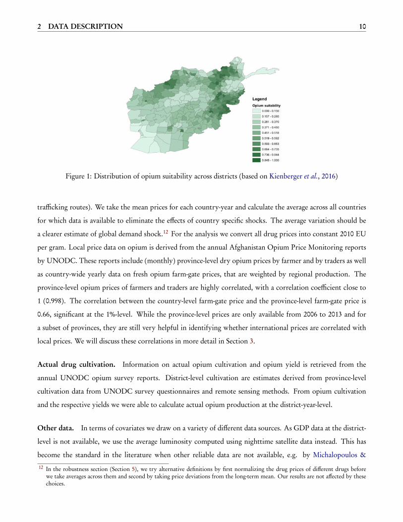
Opium suitability index. We exploit a novel data set measuring the suitability to grow opium based on
exogenous underlying information about land cover, water availability, climatic suitability, and soil suitability.
Conceptually, the index is comparable to indices on the suitability to grow other crops, which are provided by
the Food and Agricultural Organization (FAO). It was developed in the context of a study in collaboration with
UNODC, and is described in detail in a publication in a geographical science journal (Kienberger et al. 2016).
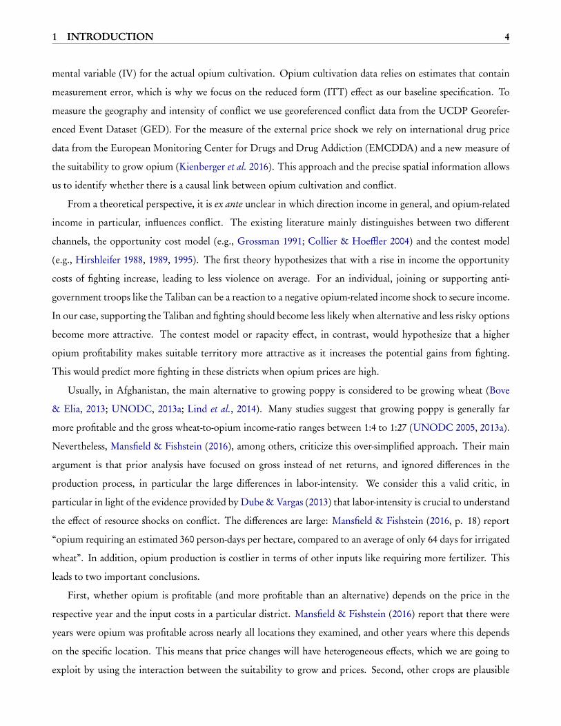
Figure 1 plots the distribution of the opium suitability index across Afghan districts. While an index of one
would indicate perfect suitability in terms of land cover, water availability, climatic suitability, and suitability of
soils, an index of zero means that the district is least suitable for growing opium. The environmental as well as
climatic suitability to cultivate opium poppy (Papaver somniferum) is characterized by different factors such as
the prevailing physio-geographical and climatic characteristics (using climatic suitability based on the EcoCrop
model from Hijmans et al. (2001)).
The data and the index itself was modeled on a 1km² resolution and then aggregated to the district units
by an area weighted mean approach. The original indicator values were normalized using a linear min–max
function between a possible value range of 0 and 100 to allow for comparison and aggregation. Only the land
cover indicator was normalized integrating expert judgments through an Analytical Hierarchy Process (AHP)
approach. The four indicators were then subsequently aggregated applying weighted means (weights were ver-
ified through expert consultations building on the AHP method). None of the input factors constituting the
index is itself to a major degree affected by conflict, which is the outcome variable. Consequently, the index
values by district can be considered as exogenously given. Given that it is generally possible to grow opium
in many parts of Afghanistan and that it is "renewable", the suitability can also be understood as the actual
"resource" that varies across districts.
Drug prices. For the measure of the external price shock we rely on international drug price data from the
European Monitoring Center for Drugs and Drug Addiction (EMCDDA). EMCDDA provides price data for
a large number of drugs in European countries (e.g., also including Turkey that is being crossed by many drug
11 The three NRVA survey waves 2005, 2007/09 and 2011/12 include between 21,000 and 31,000 households and cover 341 to 388districts of the 398 official districts in Afghanistan. The sampling design of the NRVA surveys, which is based on a two-stage clusterdesign, is done in a way that results are representative at national and provincial-level.
2 DATA DESCRIPTION 10
Figure 1: Distribution of opium suitability across districts (based on Kienberger et al., 2016)
trafficking routes). We take the mean prices for each country-year and calculate the average across all countries
for which data is available to eliminate the effects of country specific shocks. The average variation should be
a clearer estimate of global demand shock.12 For the analysis we convert all drug prices into constant 2010 EU
per gram. Local price data on opium is derived from the annual Afghanistan Opium Price Monitoring reports
by UNODC. These reports include (monthly) province-level dry opium prices by farmer and by traders as well
as country-wide yearly data on fresh opium farm-gate prices, that are weighted by regional production. The
province-level opium prices of farmers and traders are highly correlated, with a correlation coefficient close to
1 (0.998). The correlation between the country-level farm-gate price and the province-level farm-gate price is
0.66, significant at the 1%-level. While the province-level prices are only available from 2006 to 2013 and for
a subset of provinces, they are still very helpful in identifying whether international prices are correlated with
local prices. We will discuss these correlations in more detail in Section 3.
Actual drug cultivation. Information on actual opium cultivation and opium yield is retrieved from the
annual UNODC opium survey reports. District-level cultivation are estimates derived from province-level
cultivation data from UNODC survey questionnaires and remote sensing methods. From opium cultivation
and the respective yields we were able to calculate actual opium production at the district-year-level.
Other data. In terms of covariates we draw on a variety of different data sources. As GDP data at the district-
level is not available, we use the average luminosity computed using nighttime satellite data instead. This has
become the standard in the literature when other reliable data are not available, e.g. by Michalopoulos &
12 In the robustness section (Section 5), we try alternative definitions by first normalizing the drug prices of different drugs beforewe take averages across them and second by taking price deviations from the long-term mean. Our results are not affected by thesechoices.
3 IDENTIFICATION STRATEGY 11
Papaioannou (2014, 2013), and correlates strongly with changes in GDP (Henderson et al., 2012). Development
is potentially affected by our outcome variable conflict and thus endogenous, so that we will only use it as
a robustness test and always take the (pre-determined) lagged value. Population data is available at five-year
intervals. We also mainly use it in robustness tests in a lagged version as reverse causality with regard to conflict
could make it a bad control. Using district-fixed effects and only within district variation ensures that our main
estimations are not affected by differences in population size. Population data is derived using GIS software
from the Gridded Population of the World, Version 4 (GPWv4), data set. Climate conditions on the other hand
are exogenous factors that are likely to affect opium cultivation and yield. To capture inter-annual variations in
drought conditions we used the vegetation health index (VHI) provided by FAO (van Hoolst et al 2016). VHI
is an index based on earth observation data and is available on a monthly basis with a resolution of 1km². As
the opium cultivation and harvest times differ within Afghanistan, we used the yearly average of the monthly
means from March to September. We are thus able to cover the different vegetation seasons relevant for opium
poppy which starts in March in the south-western regions and ends in September in the north-western part
(UNODC 2008). Low values of the VHI indicate drought conditions. This remote sensing based index is
operationally used to monitor drought conditions in the Global Early Warning System (GEWS). The index is
thus superior to simply using precipitation data, which does not enable to directly measure drought conditions.
Using precipitation data, in particular in Afghanistan, has severe limitations in terms of quality and resolution,
and does not directly translate into actual drought conditions.13 We will use climate as an exogenous control
variable in some specifications, and as for creating additional exogenous variation in the treatment in a robustness
test. Moreover, we use additional time-invariant data on geographic conditions and further potentially relevant
factors for robustness tests. To analyze heterogeneous effects, we also georeference district-level information
about opium production and trafficking, as well as on military and government presence that are explained
in the respective section (Section 4 and 5). All variables are described with their sources in Appendix A and
descriptive statistics are reported in Appendix B.
3 Identification strategy
Our preferred specification focuses on the reduced-form intention-to-treat (ITT) effect to understand causality
in the best possible way. In addition, we use actual opium cultivation data to assess the size of our effect in
an instrumental variable setting. We prefer the first specification for two main reasons. First, cultivation data
at the district-level is an estimate derived by UNODC based on province-level data, and might thus exhibit
13 Using the VHI rather than simply precipitation is also in line with Harari & La Ferrara (2013).
3 IDENTIFICATION STRATEGY 12
considerable measurement error which would bias our estimates towards zero.14 Second, using district-level
cultivation directly in an OLS regression would obviously be highly endogenous. Using actual cultivation or
production levels would thus only allow us to identify conditional correlations, but not establish causality. To
circumvent these concerns we exploit exogenous variation in international prices that affect opium cultivation
combined with district-level data on the suitability to grow opium. Our specification and operationalization of
conflict is comparable to Berman & Couttenier (2015), and we estimate the following baseline equation at the
district-year-level over the 2002 to 2014 period:
con f l ic td,t = βopium sℎockd,t−1 + ζwℎe at sℎockd,t−1 + Xd,t−2γ + τt + δd + τt δp + εd,t , (1)
with opiumsℎockd,t−1 and wℎe at sℎockd,t−1being defined as follows:
opium sℎockd,t−1 = dr ug pr ic et−1 × opium suit abil i t yd, (2)
wℎe at sℎockd,t−1 = wℎe at pr ic et−1 × wℎe at suit abil i t yd . (3)
The outcome variable con f l ic td,t is the incidence or intensity of conflict in district d in year t based on
the different thresholds and definitions described above. The treatment variable is opium sℎockd,t−1 , which
measures the relative extent of the exogenous income shock induced by world market price changes in district
d . It is defined as the interaction of international prices dr ug pr ic et−1 with the exogenous district-specific
opium suit abil i t yd . Regarding the timing, world market sales price changes could plausibly influence opium
cultivation in the same or the following year. There are two main vegetation seasons for opium in Afghanistan,
one starting in the fall and the other in March, depending on the region (Mansfield & Fishstein, 2016). In our
preferred specification, the opium sℎock is lagged by one year. This accounts for the fact that local producers
need time to update their information set, incorporate news about price changes in the end-customer market
and adjust production. Opium production is also particularly labor-intensive in the harvesting phase towards
the end of a season. Moreover, the world market prices we use are yearly averages and could thus be influenced
by growing decisions earlier in the same year. Using one lag as a time structure is supported by Caulkins et al.
(2010, p.9 ), who writes in his book that “the largest driver of changes in hectares under poppy cultivation is not
eradication or enforcement risk, but rather last year’s opium prices.” We will also test for a contemporaneous
effect in an alternative specification shown in Appendix C.
Our main specification does not rely on control variables because the exogeneity of our opium stock should
14 As stated in UNODC (2015, 63) “District estimates are derived by a combination of different approaches. They are indicative only,and suggest a possible distribution of the estimated provincial poppy area among the districts of a province.”
3 IDENTIFICATION STRATEGY 13
not be conditional on control variables, but we will show that our results hold with and without using Xd , a
vector of district-level time-varying covariates including climate conditions, luminosity and population. Climate
conditions can also be used as contemporaneous values as they are clearly exogenous, while the other two
covariates can to some degree be endogenous to conflict.15 This is partly circumvented by using the lagged value,
assuming that we then only use the pre-determined value. Results conditioning on luminosity, population and
climate conditions are reported in Appendix D. For robustness tests, we also employ further time-invariant
covariates Xd interacted with time-fixed effects or a time trend.
We include wheat-related income shocks (wℎe at sℎockd,t−1), since wheat is the main alternative crop which
farmers grow throughout Afghanistan (Afghanistan Statistical Yearbook 2015/16). The inclusion of this vari-
able allows us to identity differential effects for the two types of income shocks, where one shock affects the
main legal and the other shock the main illegal crop. The variable wℎe at sℎockd,t−1 is defined in analogy to
opium sℎockd,t−1, where we use variation in the international wheat price interacted with the suitability to
produce wheat (wℎe at suit abil i t yd ). Since Afghanistan is not contributing by more than 1% to the global
wheat supply, we can follow the literature in taking the international price for wheat as exogenous (e.g., Berman
& Couttenier 2015). We lag the effect of wℎe at sℎock for the same reason we lag opium sℎock. Note, that our
results are not depending on the inclusion of this alternative shock.
Finally, we employ different sets of fixed effects. τt and δd are year- and district-fixed effects. District-fixed ef-
fects account for time-invariant unobservable characteristics at the district-level, and country-wide time-varying
changes are captured through time-fixed effects.The year-fixed effects for instance capture country-wide crop
diseases and changes in anti-drug policies, which affect Afghanistan as a whole. Large shares of the drugs trade
is organized at the ethnic or provincial-level, and institutions provided by ethnic groups or warlords (Giustozzi,
2009) are in many provinces more important than the central government. Accordingly, we also employ a spec-
ification that includes province-times-year-fixed effects τt δp . This is arguably a rather conservative specification,
but important as it captures, for instance, changes in conflict that are related to changes in leadership and insti-
tutions at the provincial-level, which in turn can plausibly affect conflict and drug cultivation. Identification in
this setting relies only on within-province variation in a particular year due to differences in opium suitability.
Standard errors are clustered at the district-level, but our results are robust to different choices including the
use of province-level clusters and a wild-cluster bootstrap approach that performs well for a small number of
clusters (see Table 26).
Whereas Berman & Couttenier (2015) and the majority of the literature use international prices of the
respective crop under analysis, this clearly creates an endogeneity problem in our case because Afghanistan
15 Opium eradication data provided by UNODC is only available from 2006 on and of unclear quality. We therefore do not include itin the vector of covariates. When we include eradication in year t (or in year t-1) in the regression with time- and district-fixed effectsresults remain qualitatively unchanged and significant.
3 IDENTIFICATION STRATEGY 14
cultivates a large share of the global opium production (UNODC 2013b). Conflict in Afghanistan is thus
likely to affect international opium (heroin) prices through changes in the supply of raw opium used for heroin
production. Heroin is an opiate made from morphine, which is produced from opium poppy. Usually we
would expect that more conflict leads to a decrease in supply as production becomes more difficult, which
would upward-bias estimations. It is however also possible that conflict-prone districts are less affected by anti-
drug policies (even though the extent and success of those seems limited), so that more conflict could relate to
more opium cultivation and thus results in a potential downward bias.
Our alternative identification strategy needs to fulfill two main criteria. First, we want a proxy variable for
which big supply side shocks are uncorrelated with supply side shocks for opium in Afghanistan. Second, the
proxy variable should correlate positively with the demand for opium to capture opium-related demand shocks.
In economic terms, it should be another drug for which the cross-price elasticity with opium is positive. This
means we need to identify complementary drugs for which supply side shocks are ideally exogenous to shocks
in Afghanistan. Drugs are usually classified as upper or downer drugs. Upper drugs are stimulants, and downer
drugs depressants. Heroin falls in the latter category.
There is a consensus among experts about a high share of polydrug users, i.e., users that combine two or
more different drugs. According to EMCDDA (2016) polydrug use is a common phenomenon,and a significant
number of drug users consume an upper and a downer drug. Leri et al. (2003) conclude from eight studies
in their review on heroin and cocaine co-use that the “prevalence of cocaine use among heroin addicts not in
treatment ranges from 30% to 80%” (p. 8). This can take place in form of “speed-balling” (mixing both types
of drugs, i.e., heroin and cocaine) or with some time lag (e.g. weekend versus workday drug consumption).
At least for the group of polydrug users these two types of drugs clearly constitute complements in terms of
demand. Accordingly, we expect a positive cross price-elasticity and a positive correlation in prices. We thus
take increases in the prices of three common complementary drugs cocaine, amphetamine (EMCDDA, 2016),
and ecstasy as indicating positive demand shocks for opium. Our choice of the best proxy is then a trade-off
based on the criteria outlined above.
Cocaine has the advantage that its supply is most clearly exogenous to supply shocks in Afghanistan, as
cultivation and production exclusively take place in South America. There is also nearly no overlap with regard
to trafficking routes as low cocaine seizures in Asia suggest (UNODC 2013b), so that shocks affecting drug
trafficking would not simultaneously affect the supply of both drugs. In addition, there is clear evidence of
joined consumption in the form of "speed-balling". Nevertheless, relying on one only drug price means that
due to supply side shocks for cocaine our data might contain a lot of noise, which might make it difficult to
identify a significant relationship or increase the likelihood to identify a spurious correlation.
The alternative is to form an index of the prices of all three upper drugs. The disadvantage here is that taking
3 IDENTIFICATION STRATEGY 15
-.000
50
.000
5.0
01
Index Cocaine Ecstasy Amphetamine
Lagged by 1 year
-.000
4-.0
002
0.0
002
.000
4
Index Cocaine Ecstasy Amphetamine
Lagged by 2 years
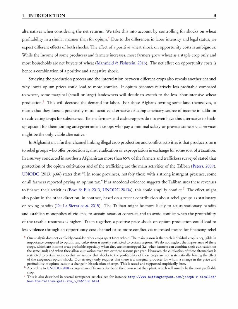
Figure 2: Correlation of opium cultivation with European drug prices
an average eliminates potentially useful variation, which might bias our results towards zero. A clear advantage,
however, is that averaging across drugs also eliminates a potential bias due to drug-specific supply side shocks
to a large extent. Given that our goal is to identify demand shocks for opium, this is an important feature of
an index. Overall, we weight the advantages of the index higher and use it for our main estimations. However,
Appendix D shows that our main results also hold when using cocaine prices only.
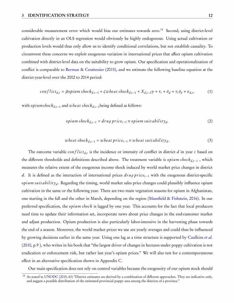
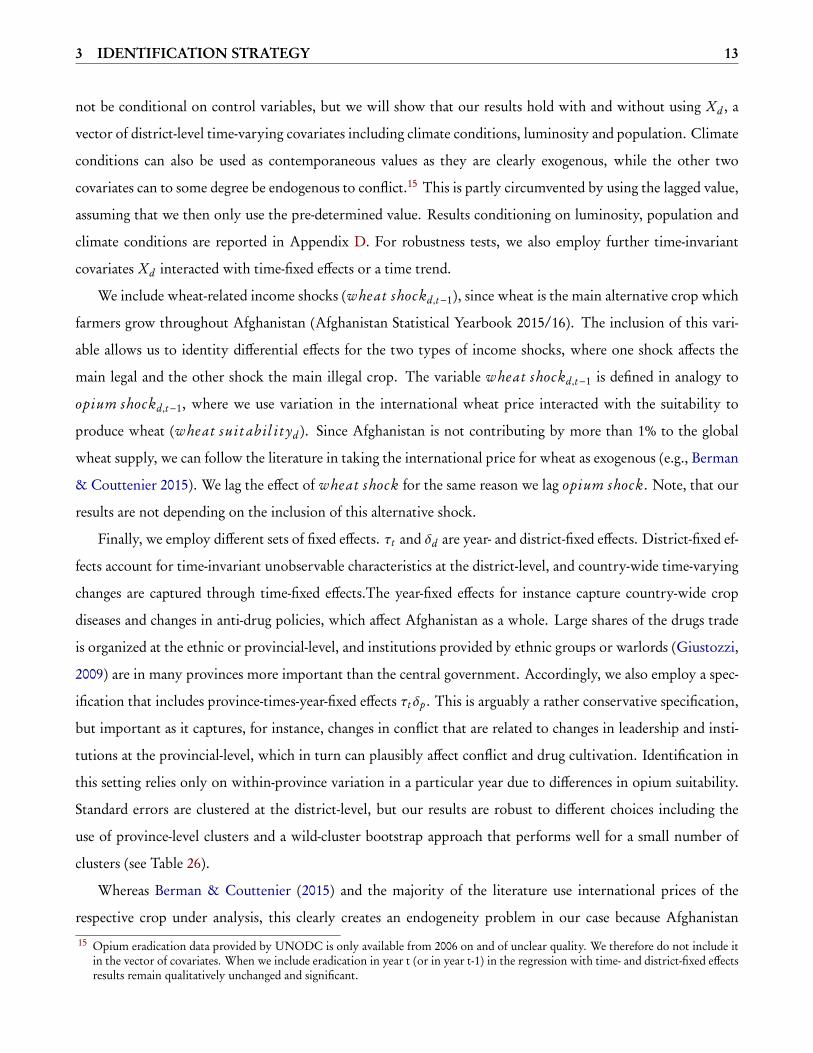
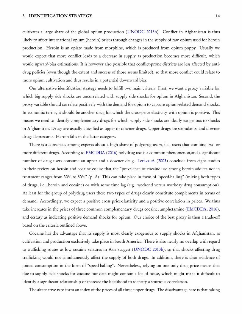
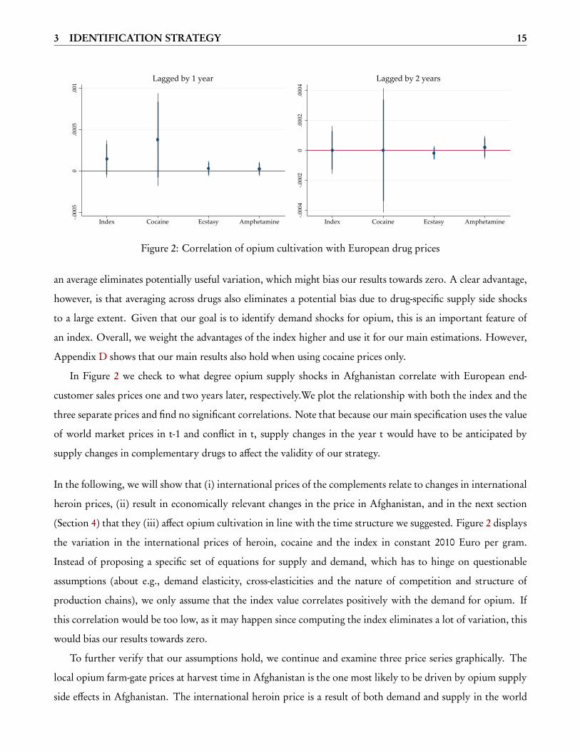
In Figure 2 we check to what degree opium supply shocks in Afghanistan correlate with European end-
customer sales prices one and two years later, respectively.We plot the relationship with both the index and the
three separate prices and find no significant correlations. Note that because our main specification uses the value
of world market prices in t-1 and conflict in t, supply changes in the year t would have to be anticipated by
supply changes in complementary drugs to affect the validity of our strategy.
In the following, we will show that (i) international prices of the complements relate to changes in international
heroin prices, (ii) result in economically relevant changes in the price in Afghanistan, and in the next section
(Section 4) that they (iii) affect opium cultivation in line with the time structure we suggested. Figure 2 displays
the variation in the international prices of heroin, cocaine and the index in constant 2010 Euro per gram.
Instead of proposing a specific set of equations for supply and demand, which has to hinge on questionable
assumptions (about e.g., demand elasticity, cross-elasticities and the nature of competition and structure of
production chains), we only assume that the index value correlates positively with the demand for opium. If
this correlation would be too low, as it may happen since computing the index eliminates a lot of variation, this
would bias our results towards zero.
To further verify that our assumptions hold, we continue and examine three price series graphically. The
local opium farm-gate prices at harvest time in Afghanistan is the one most likely to be driven by opium supply
side effects in Afghanistan. The international heroin price is a result of both demand and supply in the world
3 IDENTIFICATION STRATEGY 16
0.1
.2.3
.4.5
Afg
han
Opi
um P
rice
2040
6080
100
120
Intn
erna
tiona
l Pri
ces
2000 2005 2010 2015Year
Int. Heroin Price Int. Index PriceAfghan Opium Price
Index
0.1
.2.3
.4.5
Afg
han
Opi
um P
rice
4060
8010
012
0In
tner
natio
nal P
rice
s
2000 2005 2010 2015Year
Int. Heroin Price Int. Cocaine PriceAfghan Opium Price
Cocaine
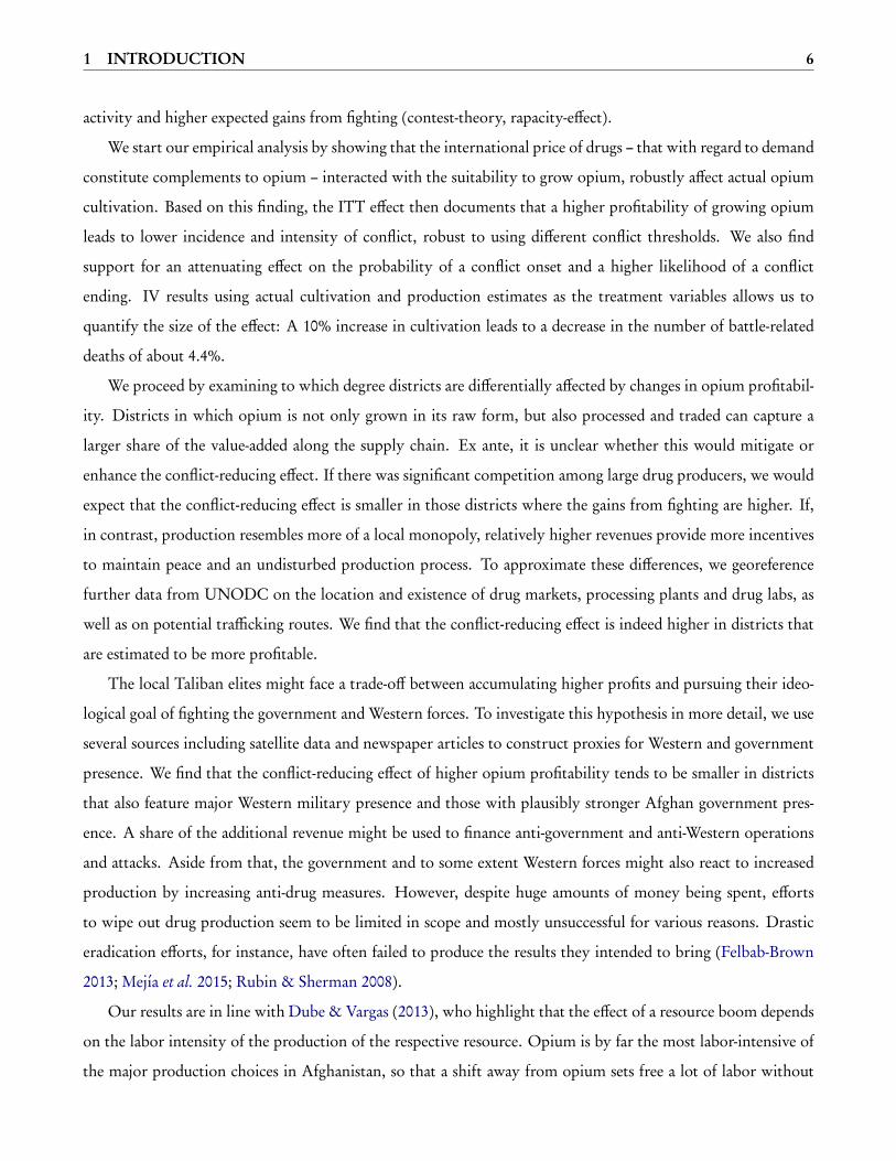
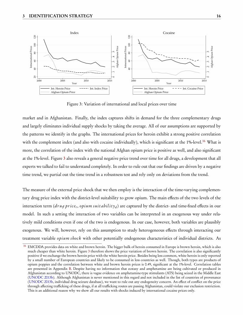
Figure 3: Variation of international and local prices over time
market and in Afghanistan. Finally, the index captures shifts in demand for the three complementary drugs
and largely eliminates individual supply shocks by taking the average. All of our assumptions are supported by
the patterns we identify in the graphs. The international prices for heroin exhibit a strong positive correlation
with the complement index (and also with cocaine individually), which is significant at the 1%-level.16 What is
more, the correlation of the index with the national Afghan opium price is positive as well, and also significant
at the 1%-level. Figure 3 also reveals a general negative price trend over time for all drugs, a development that all
experts we talked to fail to understand completely. In order to rule out that our findings are driven by a negative
time trend, we partial out the time trend in a robustness test and rely only on deviations from the trend.
The measure of the external price shock that we then employ is the interaction of the time-varying complemen-
tary drug price index with the district-level suitability to grow opium. The main effects of the two levels of the
interaction term (dr ug pr ic et , opium suit abil i t yd ) are captured by the district- and time-fixed effects in our
model. In such a setting the interaction of two variables can be interpreted in an exogenous way under rela-
tively mild conditions even if one of the two is endogenous. In our case, however, both variables are plausibly
exogenous. We will, however, rely on this assumption to study heterogeneous effects through interacting our
treatment variable opium sℎock with other potentially endogenous characteristics of individual districts. As
16 EMCDDA provides data on white and brown heroin. The bigger bulk of heroin consumed in Europe is brown heroin, which is alsomuch cheaper than white heroin. Figure 3 therefore shows the price variation of brown heroin. The correlation is also significantlypositive if we exchange the brown heroin price with the white heroin price. Besides being less common, white heroin is only reportedby a small number of European countries and likely to be consumed in less countries as well. Though, both types are products ofopium poppies and the correlation between white and brown heroin prices is 0.49, significant at the 1%-level. Correlation tablesare presented in Appendix B. Despite having no information that ecstasy and amphetamine are being cultivated or produced inAfghanistan according to UNODC, there is vague evidence on amphetamine-type stimulants (ATS) being seized in the Middle East(UNODC 2013b). Although Afghanistan is never mentioned in this regard and not included in the list of countries of provenance(UNODC 2013b, individual drug seizure database), we want to rule out any endogeneity concern. An effect of conflict on the pricethrough affecting trafficking of these drugs, if at all trafficking routes are passing Afghanistan, could violate our exclusion restriction.This is an additional reason why we show all our results with shocks induced by international cocaine prices only.
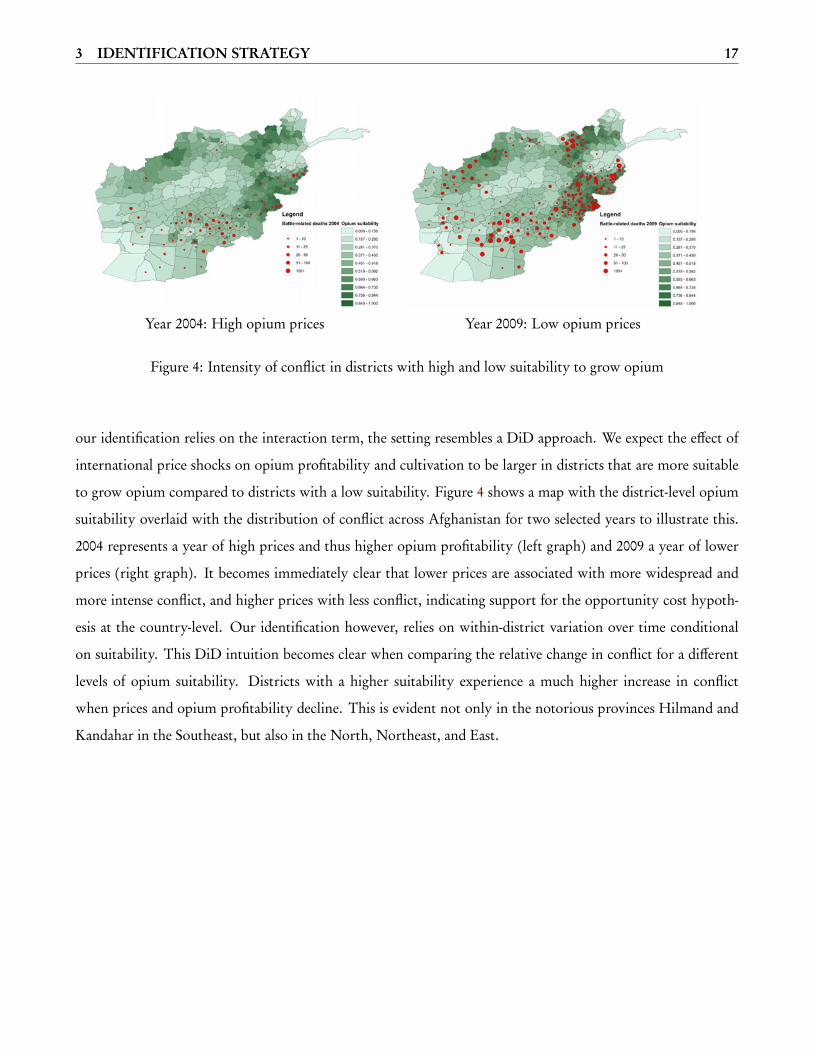
3 IDENTIFICATION STRATEGY 17
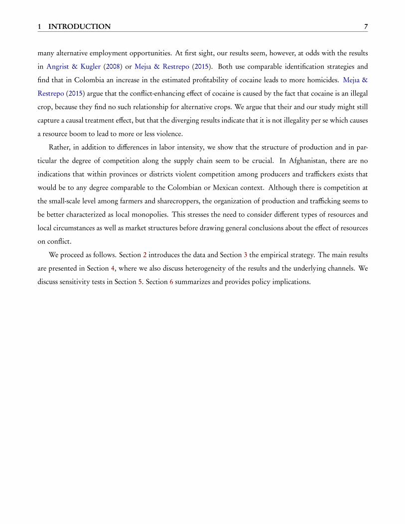
Year 2004: High opium prices Year 2009: Low opium prices
Figure 4: Intensity of conflict in districts with high and low suitability to grow opium
our identification relies on the interaction term, the setting resembles a DiD approach. We expect the effect of
international price shocks on opium profitability and cultivation to be larger in districts that are more suitable
to grow opium compared to districts with a low suitability. Figure 4 shows a map with the district-level opium
suitability overlaid with the distribution of conflict across Afghanistan for two selected years to illustrate this.
2004 represents a year of high prices and thus higher opium profitability (left graph) and 2009 a year of lower
prices (right graph). It becomes immediately clear that lower prices are associated with more widespread and
more intense conflict, and higher prices with less conflict, indicating support for the opportunity cost hypoth-
esis at the country-level. Our identification however, relies on within-district variation over time conditional
on suitability. This DiD intuition becomes clear when comparing the relative change in conflict for a different
levels of opium suitability. Districts with a higher suitability experience a much higher increase in conflict
when prices and opium profitability decline. This is evident not only in the notorious provinces Hilmand and
Kandahar in the Southeast, but also in the North, Northeast, and East.
4 RESULTS 18
4 Results
4.1 International prices and opium cultivation
After showing that the international price index is indeed positively correlated with the international heroin
and the local opium price, we proceed and test whether the index really captures demand shocks for opium
that translate into changes in actual opium cultivation at the district-level in Afghanistan. We therefore run
the empirical model as defined in equation (1) but with the actual opium cultivation and revenues from opium
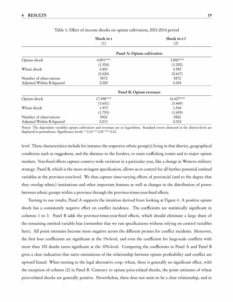
cultivation (both in logarithms) as the dependent variables. Table 1 presents the results for opium cultivation in
Panel A and opium revenues in Panel B. Opium revenues are defined as the production in kg multiplied with the
Afghan opium farm-gate price at harvest in constant 2010 EU/kg. We see that external price shocks, measured
by the interaction of international prices of upper drugs with the suitability to grow opium, lead to an increase
in actual opium cultivation and opium revenues. This holds both when using the value in t-1, as well as when
using the potentially more difficult contemporaneous value. These results are significant at the 1%-level. It is
also reassuring that the wheat shock, which can also be interpreted as a kind of placebo test here, has no effect
on opium cultivation and revenues.
Quantitatively, a 1% increase in the price leads to about a 4 to 5% increase in cultivation for those districts
where opium suitability reaches one (perfect suitability). For districts characterized by the mean suitability
(0.51) the effect would roughly decrease by half (0.51*3.850 to 0.51*4.891) but the elasticity is still bigger than
one. The same increase in prices would lead to a 14.5 to 17.5% increase in opium revenues in districts with the
highest possible suitability to grow opium. This estimation does not include province-times-year-fixed effects as
the actual cultivation data is gathered at the province-level and we only estimated it for the district-level. Note
that the results are robust to changing 1) the definition of the dependent variable and 2) the definition of the
price shock including the exchange of the index with the cocaine price. Based on this evidence we are convinced
of the validity of our strategy and proceed with estimating the effect on conflict.
4.2 Main results
We now turn to our main results, where we start with the effect of income shocks on the incidence of conflict.
Table 2 is structured as follows. In Panel A we report the baseline results with year- and district-fixed effects only
and Panel B adds province-times-year-fixed effects. We report results for different dependent variables, where
column (1) uses the continuous measure (log of BRD), columns (2) to (5) define conflict as a binary indicator
with increasing thresholds of BRD. Panel A allows to control for time-invariant characteristics at the district-
4 RESULTS 19
Table 1: Effect of income shocks on opium cultivation, 2001-2014 period
Shock in t Shock in t-1(1) (2)
Panel A: Opium cultivation
Opium shock 4.891*** 3.850***(1.304) (1.250)
Wheat shock 0.801 0.583(0.624) (0.617)
Number of observations 5572 5572Adjusted Within R-Squared 0.005 0.004
Panel B: Opium revenues
Opium shock 17.498*** 14.427***(3.651) (3.469)
Wheat shock 1.973 1.544(1.753) (1.659)
Number of observations 5502 5502Adjusted Within R-Squared 0.011 0.010Notes: The dependent variables opium cultivation and revenues are in logarithms. Standard errors clustered at the district-level aredisplayed in parentheses. Significance levels: * 0.10 ** 0.05 *** 0.01.
level. These characteristics include for instance the respective ethnic group(s) living in that district, geographical
conditions such as ruggedness, and the distance to the borders, to main trafficking routes and to major opium
markets. Year-fixed effects capture country-wide variation in a particular year, like a change in Western military
strategy. Panel B, which is the more stringent specification, allows us to control for all further potential omitted
variables at the province-year-level. We thus capture time-varying effects of provincial (and to the degree that
they overlap ethnic) institutions and other important features as well as changes in the distribution of power
between ethnic groups within a province through the province-times-year-fixed effects.
Turning to our results, Panel A supports the intuition derived from looking at Figure 4. A positive opium
shock has a consistently negative effect on conflict incidence. The coefficients are statistically significant in
columns 1 to 3. Panel B adds the province-times-year-fixed effects, which should eliminate a large share of
the remaining omitted variable bias (remember that we run specifications without relying on control variables
here). All point estimates become more negative across the different proxies for conflict incidents. Moreover,
the first four coefficients are significant at the 1%-level, and even the coefficient for large-scale conflicts with
more than 100 deaths turns significant at the 10%-level. Comparing the coefficients in Panel A and Panel B
gives a clear indication that naive estimations of the relationship between opium profitability and conflict are
upward biased. When turning to the legal alternative crop, wheat, there is generally no significant effect, with
the exception of column (2) in Panel B. Contrary to opium price-related shocks, the point estimates of wheat
price-related shocks are generally positive. Nevertheless, there does not seem to be a clear relationship, and in
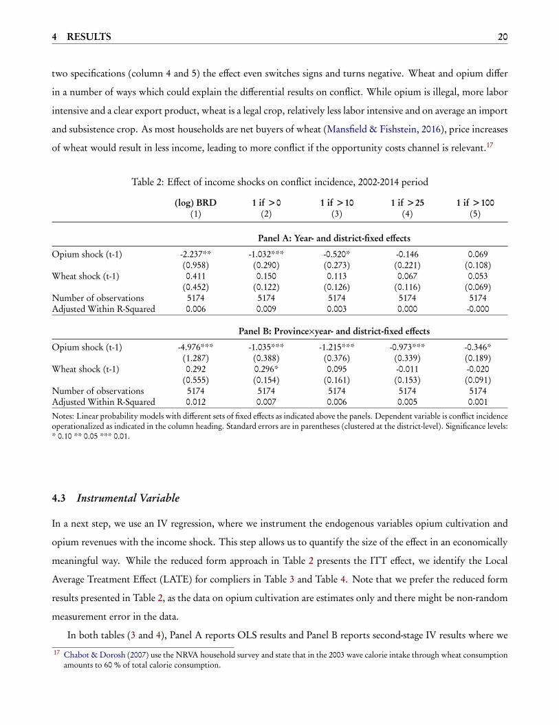
4 RESULTS 20
two specifications (column 4 and 5) the effect even switches signs and turns negative. Wheat and opium differ
in a number of ways which could explain the differential results on conflict. While opium is illegal, more labor
intensive and a clear export product, wheat is a legal crop, relatively less labor intensive and on average an import
and subsistence crop. As most households are net buyers of wheat (Mansfield & Fishstein, 2016), price increases
of wheat would result in less income, leading to more conflict if the opportunity costs channel is relevant.17
Table 2: Effect of income shocks on conflict incidence, 2002-2014 period
(log) BRD 1 if >0 1 if >10 1 if >25 1 if >100(1) (2) (3) (4) (5)
Panel A: Year- and district-fixed effects
Opium shock (t-1) -2.237** -1.032*** -0.520* -0.146 0.069(0.958) (0.290) (0.273) (0.221) (0.108)
Wheat shock (t-1) 0.411 0.150 0.113 0.067 0.053(0.452) (0.122) (0.126) (0.116) (0.069)
Number of observations 5174 5174 5174 5174 5174Adjusted Within R-Squared 0.006 0.009 0.003 0.000 -0.000
Panel B: Province×year- and district-fixed effects
Opium shock (t-1) -4.976*** -1.035*** -1.215*** -0.973*** -0.346*(1.287) (0.388) (0.376) (0.339) (0.189)
Wheat shock (t-1) 0.292 0.296* 0.095 -0.011 -0.020(0.555) (0.154) (0.161) (0.153) (0.091)
Number of observations 5174 5174 5174 5174 5174Adjusted Within R-Squared 0.012 0.007 0.006 0.005 0.001Notes: Linear probability models with different sets of fixed effects as indicated above the panels. Dependent variable is conflict incidenceoperationalized as indicated in the column heading. Standard errors are in parentheses (clustered at the district-level). Significance levels:* 0.10 ** 0.05 *** 0.01.
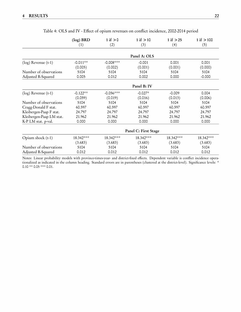
4.3 Instrumental Variable
In a next step, we use an IV regression, where we instrument the endogenous variables opium cultivation and
opium revenues with the income shock. This step allows us to quantify the size of the effect in an economically
meaningful way. While the reduced form approach in Table 2 presents the ITT effect, we identify the Local
Average Treatment Effect (LATE) for compliers in Table 3 and Table 4. Note that we prefer the reduced form
results presented in Table 2, as the data on opium cultivation are estimates only and there might be non-random
measurement error in the data.
In both tables (3 and 4), Panel A reports OLS results and Panel B reports second-stage IV results where we
17 Chabot & Dorosh (2007) use the NRVA household survey and state that in the 2003 wave calorie intake through wheat consumptionamounts to 60 % of total calorie consumption.
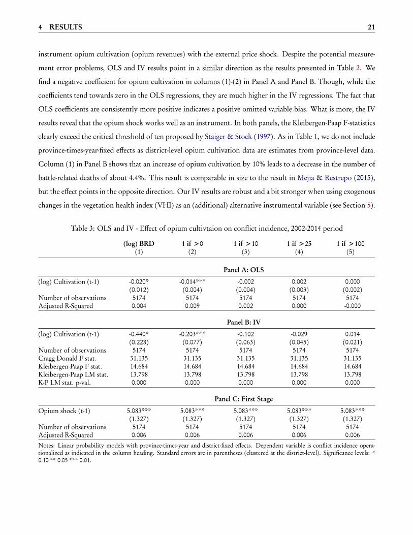
4 RESULTS 21
instrument opium cultivation (opium revenues) with the external price shock. Despite the potential measure-
ment error problems, OLS and IV results point in a similar direction as the results presented in Table 2. We
find a negative coefficient for opium cultivation in columns (1)-(2) in Panel A and Panel B. Though, while the
coefficients tend towards zero in the OLS regressions, they are much higher in the IV regressions. The fact that
OLS coefficients are consistently more positive indicates a positive omitted variable bias. What is more, the IV
results reveal that the opium shock works well as an instrument. In both panels, the Kleibergen-Paap F-statistics
clearly exceed the critical threshold of ten proposed by Staiger & Stock (1997). As in Table 1, we do not include
province-times-year-fixed effects as district-level opium cultivation data are estimates from province-level data.
Column (1) in Panel B shows that an increase of opium cultivation by 10% leads to a decrease in the number of
battle-related deaths of about 4.4%. This result is comparable in size to the result in Mejıa & Restrepo (2015),
but the effect points in the opposite direction. Our IV results are robust and a bit stronger when using exogenous
changes in the vegetation health index (VHI) as an (additional) alternative instrumental variable (see Section 5).
Table 3: OLS and IV - Effect of opium cultivtaion on conflict incidence, 2002-2014 period
(log) BRD 1 if >0 1 if >10 1 if >25 1 if >100(1) (2) (3) (4) (5)
Panel A: OLS
(log) Cultivation (t-1) -0.020* -0.014*** -0.002 0.002 0.000(0.012) (0.004) (0.004) (0.003) (0.002)
Number of observations 5174 5174 5174 5174 5174Adjusted R-Squared 0.004 0.009 0.002 0.000 -0.000
Panel B: IV
(log) Cultivation (t-1) -0.440* -0.203*** -0.102 -0.029 0.014(0.228) (0.077) (0.063) (0.045) (0.021)
Number of observations 5174 5174 5174 5174 5174Cragg-Donald F stat. 31.135 31.135 31.135 31.135 31.135Kleibergen-Paap F stat. 14.684 14.684 14.684 14.684 14.684Kleibergen-Paap LM stat. 13.798 13.798 13.798 13.798 13.798K-P LM stat. p-val. 0.000 0.000 0.000 0.000 0.000
Panel C: First Stage
Opium shock (t-1) 5.083*** 5.083*** 5.083*** 5.083*** 5.083***(1.327) (1.327) (1.327) (1.327) (1.327)
Number of observations 5174 5174 5174 5174 5174Adjusted R-Squared 0.006 0.006 0.006 0.006 0.006Notes: Linear probability models with province-times-year and district-fixed effects. Dependent variable is conflict incidence opera-tionalized as indicated in the column heading. Standard errors are in parentheses (clustered at the district-level). Significance levels: *0.10 ** 0.05 *** 0.01.
4 RESULTS 22
Table 4: OLS and IV - Effect of opium revenues on conflict incidence, 2002-2014 period
(log) BRD 1 if >0 1 if >10 1 if >25 1 if >100(1) (2) (3) (4) (5)
Panel A: OLS(log) Revenue (t-1) -0.011** -0.008*** -0.001 0.001 0.001
(0.005) (0.002) (0.001) (0.001) (0.000)Number of observations 5104 5104 5104 5104 5104Adjusted R-Squared 0.005 0.012 0.002 0.000 -0.000
Panel B: IV
(log) Revenue (t-1) -0.122** -0.056*** -0.027* -0.009 0.004(0.059) (0.019) (0.016) (0.013) (0.006)
Number of observations 5104 5104 5104 5104 5104Cragg-Donald F stat. 60.597 60.597 60.597 60.597 60.597Kleibergen-Paap F stat. 24.797 24.797 24.797 24.797 24.797Kleibergen-Paap LM stat. 21.962 21.962 21.962 21.962 21.962K-P LM stat. p-val. 0.000 0.000 0.000 0.000 0.000
Panel C: First Stage
Opium shock (t-1) 18.342*** 18.342*** 18.342*** 18.342*** 18.342***(3.683) (3.683) (3.683) (3.683) (3.683)
Number of observations 5104 5104 5104 5104 5104Adjusted R-Squared 0.012 0.012 0.012 0.012 0.012Notes: Linear probability models with province-times-year- and district-fixed effects. Dependent variable is conflict incidence opera-tionalized as indicated in the column heading. Standard errors are in parentheses (clustered at the district-level). Significance levels: *0.10 ** 0.05 *** 0.01.
4 RESULTS 23
Taken together, we find that positive income shocks are important determinants of conflict incidence in the
ITT and IV estimation. The effects are stronger and more robust for income shocks relating to opium cultiva-
tion, and we find no such relationship for shocks relating to wheat as one main legal alternative. The results
are robust to a) using different conflict measures, b) altering the definition of the income shock including the
exchange of the price index with the price of cocaine, c) different lag structures including contemporaneous
effects, d) including covariates and trends, e) adjusting how we cluster the standard error, and f) different em-
pirical models.18 Our findings are in line with the results for positive income shocks in Berman et al. (2010)
and they support the conclusions in Dube & Vargas (2013) that the labor intensity of a resource compared to
counterfactual alternatives is a decisive factor. However, our results are at odds with conclusion in Mejıa &
Restrepo (2015) that an income shock for an illegal resource is related to more conflict. While coca has a similar
labor intensity as the alternative crops cacao, palm oil, and sugar cane in Colombia (Mejıa & Restrepo, 2015),
opium cultivation is much more labor-intensive then all alternative crops. The next section will elaborate more
on why this context differs, and why illegality per se is not the decisive factor moderating the effect on conflict.
4.4 Mechanisms and transmission channels
This section examines to which degree the effect of opium production on conflict depends on particular features
of a district. We are interested in examining how the relationship between opium and conflict is moderated by
factors relating to the share of value-added along the production chain of a district, and by variables indicating
the presence of government institutions and Western forces. This should help us to better understand the role of
local market conditions, identify important actors and their incentives, and potential trade-offs between lucrative
drug production and ideologically driven conflict activities. For this endeavor, we georeference data on whether
a district contains a heroin or morphine lab, an opium market (major or sub-market), whether it is crossed by
potential drug trafficking routes, and if it features an unofficial border-crossing point used for smuggling drugs
out of the country. Profit margins are higher further up the production chain, markets create more jobs and
additional revenue, and trafficking routes and border-crossings allow the local leaders to raise income through
some form of taxation or road charges.
To approximate the strength of government institutions and the presence of Western military, we compute
distances to the seat of government and assemble information about military camps and Western casualties.
Lind et al. (2014) also uses the distance to Kabul as an indicator for low governmental law enforcement and
weak institutions. We also include information on whether the ethnic group of Pashtuns is present in a district,
and whether the district has been controlled by the Taliban in 1996 (Dorronsoro, 2005). There is no available
reliable time-varying data about Taliban-dominated territory. Moreover, current control would of course be18 Results on robustness tests are presented in Appendix D.
4 RESULTS 24
highly endogenous. Accordingly, we prefer to rely on variation determined before our observation period. In
both types of districts we expect government institutions to be potentially less strong. Anecdotal evidence and
personal conversations with experts suggest that ethnic institutions are more relevant in Pashtun areas. For
areas formerly under Taliban control we would expect that due to the common past the Taliban could face less
resistance (of course not everywhere). We use a variety of different sources to code these variables, ranging from
maps provided by experts at the United Nations, to American military data, satellite images and newspaper
reports to confirm the presence of a military camp in a particular district. Appendix F documents the steps
involved in the construction of all variables and its sources in detail.
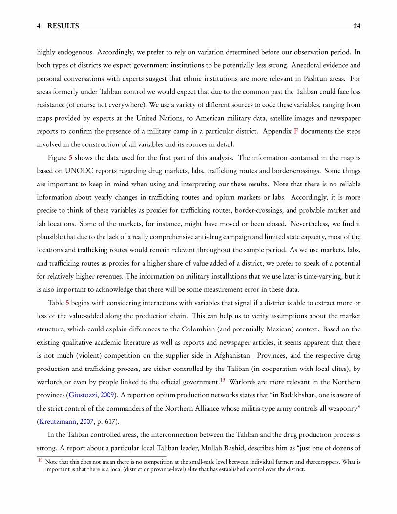
Figure 5 shows the data used for the first part of this analysis. The information contained in the map is
based on UNODC reports regarding drug markets, labs, trafficking routes and border-crossings. Some things
are important to keep in mind when using and interpreting our these results. Note that there is no reliable
information about yearly changes in trafficking routes and opium markets or labs. Accordingly, it is more
precise to think of these variables as proxies for trafficking routes, border-crossings, and probable market and
lab locations. Some of the markets, for instance, might have moved or been closed. Nevertheless, we find it
plausible that due to the lack of a really comprehensive anti-drug campaign and limited state capacity, most of the
locations and trafficking routes would remain relevant throughout the sample period. As we use markets, labs,
and trafficking routes as proxies for a higher share of value-added of a district, we prefer to speak of a potential
for relatively higher revenues. The information on military installations that we use later is time-varying, but it
is also important to acknowledge that there will be some measurement error in these data.
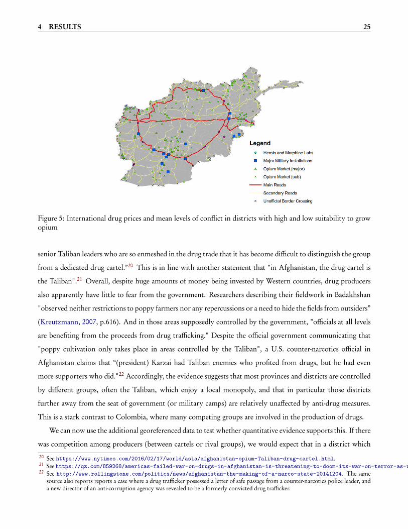
Table 5 begins with considering interactions with variables that signal if a district is able to extract more or
less of the value-added along the production chain. This can help us to verify assumptions about the market
structure, which could explain differences to the Colombian (and potentially Mexican) context. Based on the
existing qualitative academic literature as well as reports and newspaper articles, it seems apparent that there
is not much (violent) competition on the supplier side in Afghanistan. Provinces, and the respective drug
production and trafficking process, are either controlled by the Taliban (in cooperation with local elites), by
warlords or even by people linked to the official government.19 Warlords are more relevant in the Northern
provinces (Giustozzi, 2009). A report on opium production networks states that “in Badakhshan, one is aware of
the strict control of the commanders of the Northern Alliance whose militia-type army controls all weaponry”
(Kreutzmann, 2007, p. 617).
In the Taliban controlled areas, the interconnection between the Taliban and the drug production process is
strong. A report about a particular local Taliban leader, Mullah Rashid, describes him as “just one of dozens of
19 Note that this does not mean there is no competition at the small-scale level between individual farmers and sharecroppers. What isimportant is that there is a local (district or province-level) elite that has established control over the district.
4 RESULTS 25
Figure 5: International drug prices and mean levels of conflict in districts with high and low suitability to growopium
senior Taliban leaders who are so enmeshed in the drug trade that it has become difficult to distinguish the group
from a dedicated drug cartel.”20 This is in line with another statement that "in Afghanistan, the drug cartel is
the Taliban".21 Overall, despite huge amounts of money being invested by Western countries, drug producers
also apparently have little to fear from the government. Researchers describing their fieldwork in Badakhshan
"observed neither restrictions to poppy farmers nor any repercussions or a need to hide the fields from outsiders”
(Kreutzmann, 2007, p.616). And in those areas supposedly controlled by the government, "officials at all levels
are benefiting from the proceeds from drug trafficking." Despite the official government communicating that
"poppy cultivation only takes place in areas controlled by the Taliban", a U.S. counter-narcotics official in
Afghanistan claims that “(president) Karzai had Taliban enemies who profited from drugs, but he had even
more supporters who did."22 Accordingly, the evidence suggests that most provinces and districts are controlled
by different groups, often the Taliban, which enjoy a local monopoly, and that in particular those districts
further away from the seat of government (or military camps) are relatively unaffected by anti-drug measures.
This is a stark contrast to Colombia, where many competing groups are involved in the production of drugs.
We can now use the additional georeferenced data to test whether quantitative evidence supports this. If there
was competition among producers (between cartels or rival groups), we would expect that in a district which
20 See https://www.nytimes.com/2016/02/17/world/asia/afghanistan-opium-Taliban-drug-cartel.html.21 See https://qz.com/859268/americas-failed-war-on-drugs-in-afghanistan-is-threatening-to-doom-its-war-on-terror-as-well/.22 See http://www.rollingstone.com/politics/news/afghanistan-the-making-of-a-narco-state-20141204. The same
source also reports reports a case where a drug trafficker possessed a letter of safe passage from a counter-narcotics police leader, anda new director of an anti-corruption agency was revealed to be a formerly convicted drug trafficker.
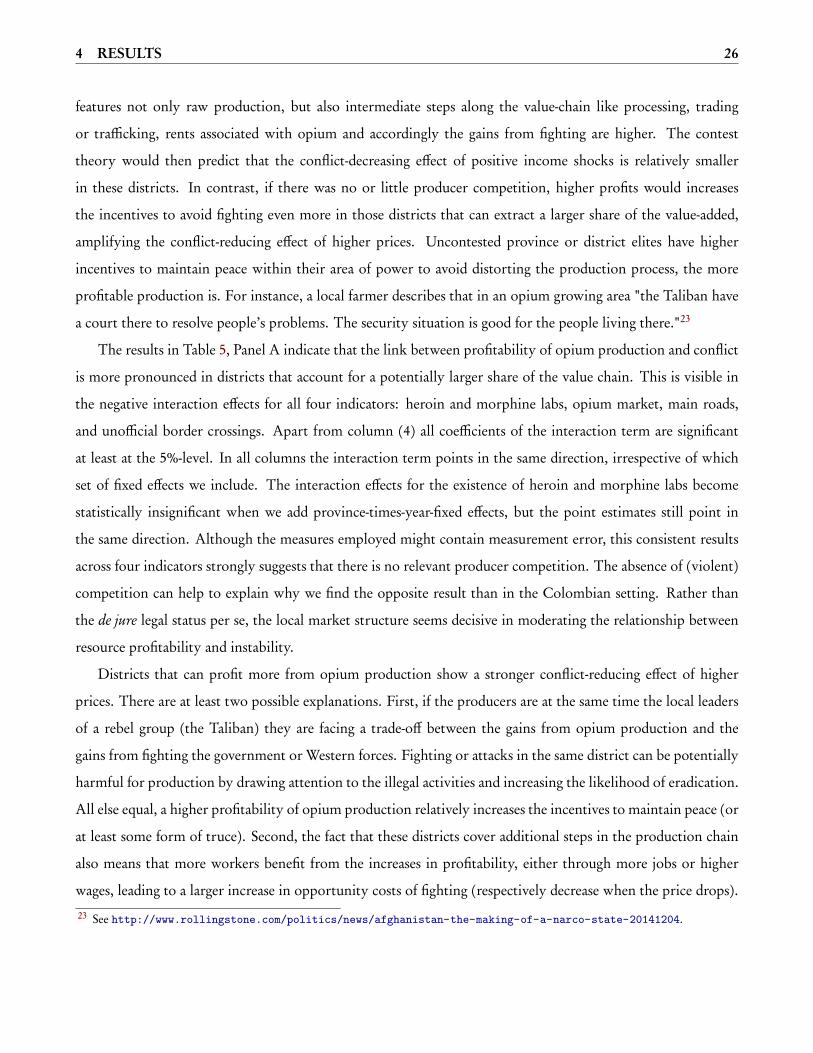
4 RESULTS 26
features not only raw production, but also intermediate steps along the value-chain like processing, trading
or trafficking, rents associated with opium and accordingly the gains from fighting are higher. The contest
theory would then predict that the conflict-decreasing effect of positive income shocks is relatively smaller
in these districts. In contrast, if there was no or little producer competition, higher profits would increases
the incentives to avoid fighting even more in those districts that can extract a larger share of the value-added,
amplifying the conflict-reducing effect of higher prices. Uncontested province or district elites have higher
incentives to maintain peace within their area of power to avoid distorting the production process, the more
profitable production is. For instance, a local farmer describes that in an opium growing area "the Taliban have
a court there to resolve people’s problems. The security situation is good for the people living there."23
The results in Table 5, Panel A indicate that the link between profitability of opium production and conflict
is more pronounced in districts that account for a potentially larger share of the value chain. This is visible in
the negative interaction effects for all four indicators: heroin and morphine labs, opium market, main roads,
and unofficial border crossings. Apart from column (4) all coefficients of the interaction term are significant
at least at the 5%-level. In all columns the interaction term points in the same direction, irrespective of which
set of fixed effects we include. The interaction effects for the existence of heroin and morphine labs become
statistically insignificant when we add province-times-year-fixed effects, but the point estimates still point in
the same direction. Although the measures employed might contain measurement error, this consistent results
across four indicators strongly suggests that there is no relevant producer competition. The absence of (violent)
competition can help to explain why we find the opposite result than in the Colombian setting. Rather than
the de jure legal status per se, the local market structure seems decisive in moderating the relationship between
resource profitability and instability.
Districts that can profit more from opium production show a stronger conflict-reducing effect of higher
prices. There are at least two possible explanations. First, if the producers are at the same time the local leaders
of a rebel group (the Taliban) they are facing a trade-off between the gains from opium production and the
gains from fighting the government or Western forces. Fighting or attacks in the same district can be potentially
harmful for production by drawing attention to the illegal activities and increasing the likelihood of eradication.
All else equal, a higher profitability of opium production relatively increases the incentives to maintain peace (or
at least some form of truce). Second, the fact that these districts cover additional steps in the production chain
also means that more workers benefit from the increases in profitability, either through more jobs or higher
wages, leading to a larger increase in opportunity costs of fighting (respectively decrease when the price drops).
23 See http://www.rollingstone.com/politics/news/afghanistan-the-making-of-a-narco-state-20141204.
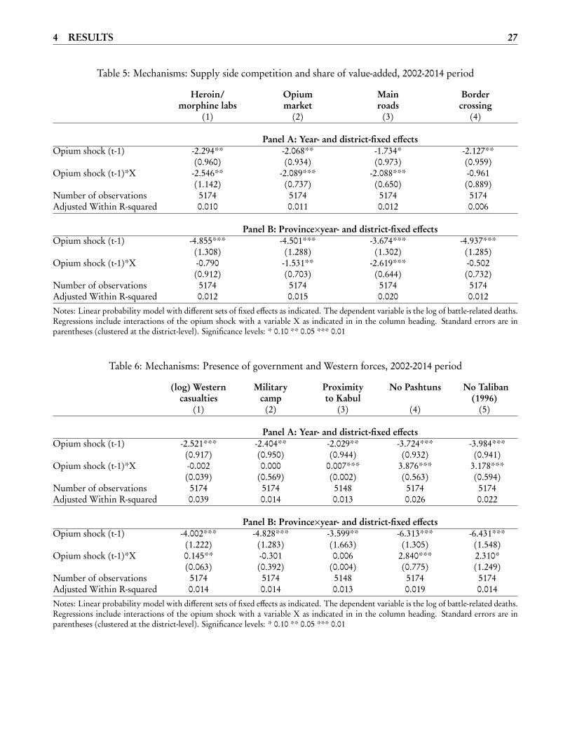
4 RESULTS 27
Table 5: Mechanisms: Supply side competition and share of value-added, 2002-2014 period
Heroin/ Opium Main Bordermorphine labs market roads crossing
(1) (2) (3) (4)
Panel A: Year- and district-fixed effectsOpium shock (t-1) -2.294** -2.068** -1.734* -2.127**
(0.960) (0.934) (0.973) (0.959)Opium shock (t-1)*X -2.546** -2.089*** -2.088*** -0.961
(1.142) (0.737) (0.650) (0.889)Number of observations 5174 5174 5174 5174Adjusted Within R-squared 0.010 0.011 0.012 0.006
Panel B: Province×year- and district-fixed effectsOpium shock (t-1) -4.855*** -4.501*** -3.674*** -4.937***
(1.308) (1.288) (1.302) (1.285)Opium shock (t-1)*X -0.790 -1.531** -2.619*** -0.502
(0.912) (0.703) (0.644) (0.732)Number of observations 5174 5174 5174 5174Adjusted Within R-squared 0.012 0.015 0.020 0.012Notes: Linear probability model with different sets of fixed effects as indicated. The dependent variable is the log of battle-related deaths.Regressions include interactions of the opium shock with a variable X as indicated in in the column heading. Standard errors are inparentheses (clustered at the district-level). Significance levels: * 0.10 ** 0.05 *** 0.01
Table 6: Mechanisms: Presence of government and Western forces, 2002-2014 period
(log) Western Military Proximity No Pashtuns No Talibancasualties camp to Kabul (1996)
(1) (2) (3) (4) (5)
Panel A: Year- and district-fixed effectsOpium shock (t-1) -2.521*** -2.404** -2.029** -3.724*** -3.984***
(0.917) (0.950) (0.944) (0.932) (0.941)Opium shock (t-1)*X -0.002 0.000 0.007*** 3.876*** 3.178***
(0.039) (0.569) (0.002) (0.563) (0.594)Number of observations 5174 5174 5148 5174 5174Adjusted Within R-squared 0.039 0.014 0.013 0.026 0.022
Panel B: Province×year- and district-fixed effectsOpium shock (t-1) -4.002*** -4.828*** -3.599** -6.313*** -6.431***
(1.222) (1.283) (1.663) (1.305) (1.548)Opium shock (t-1)*X 0.145** -0.301 0.006 2.840*** 2.310*
(0.063) (0.392) (0.004) (0.775) (1.249)Number of observations 5174 5174 5148 5174 5174Adjusted Within R-squared 0.014 0.014 0.013 0.019 0.014Notes: Linear probability model with different sets of fixed effects as indicated. The dependent variable is the log of battle-related deaths.Regressions include interactions of the opium shock with a variable X as indicated in in the column heading. Standard errors are inparentheses (clustered at the district-level). Significance levels: * 0.10 ** 0.05 *** 0.01
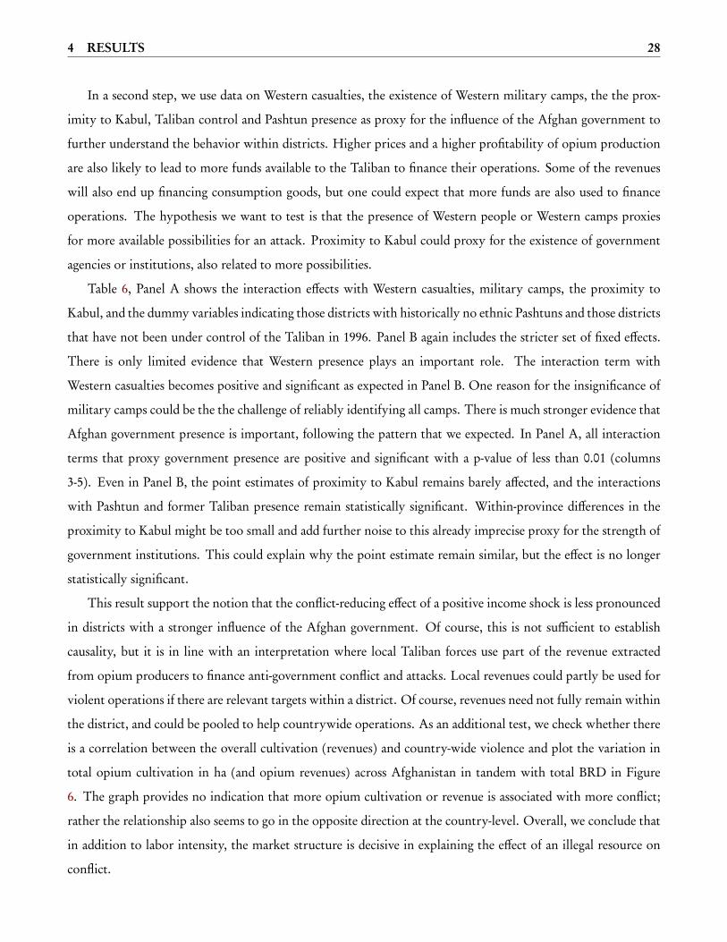
4 RESULTS 28
In a second step, we use data on Western casualties, the existence of Western military camps, the the prox-
imity to Kabul, Taliban control and Pashtun presence as proxy for the influence of the Afghan government to
further understand the behavior within districts. Higher prices and a higher profitability of opium production
are also likely to lead to more funds available to the Taliban to finance their operations. Some of the revenues
will also end up financing consumption goods, but one could expect that more funds are also used to finance
operations. The hypothesis we want to test is that the presence of Western people or Western camps proxies
for more available possibilities for an attack. Proximity to Kabul could proxy for the existence of government
agencies or institutions, also related to more possibilities.
Table 6, Panel A shows the interaction effects with Western casualties, military camps, the proximity to
Kabul, and the dummy variables indicating those districts with historically no ethnic Pashtuns and those districts
that have not been under control of the Taliban in 1996. Panel B again includes the stricter set of fixed effects.
There is only limited evidence that Western presence plays an important role. The interaction term with
Western casualties becomes positive and significant as expected in Panel B. One reason for the insignificance of
military camps could be the the challenge of reliably identifying all camps. There is much stronger evidence that
Afghan government presence is important, following the pattern that we expected. In Panel A, all interaction
terms that proxy government presence are positive and significant with a p-value of less than 0.01 (columns
3-5). Even in Panel B, the point estimates of proximity to Kabul remains barely affected, and the interactions
with Pashtun and former Taliban presence remain statistically significant. Within-province differences in the
proximity to Kabul might be too small and add further noise to this already imprecise proxy for the strength of
government institutions. This could explain why the point estimate remain similar, but the effect is no longer
statistically significant.
This result support the notion that the conflict-reducing effect of a positive income shock is less pronounced
in districts with a stronger influence of the Afghan government. Of course, this is not sufficient to establish
causality, but it is in line with an interpretation where local Taliban forces use part of the revenue extracted
from opium producers to finance anti-government conflict and attacks. Local revenues could partly be used for
violent operations if there are relevant targets within a district. Of course, revenues need not fully remain within
the district, and could be pooled to help countrywide operations. As an additional test, we check whether there
is a correlation between the overall cultivation (revenues) and country-wide violence and plot the variation in
total opium cultivation in ha (and opium revenues) across Afghanistan in tandem with total BRD in Figure
6. The graph provides no indication that more opium cultivation or revenue is associated with more conflict;
rather the relationship also seems to go in the opposite direction at the country-level. Overall, we conclude that
in addition to labor intensity, the market structure is decisive in explaining the effect of an illegal resource on
conflict.
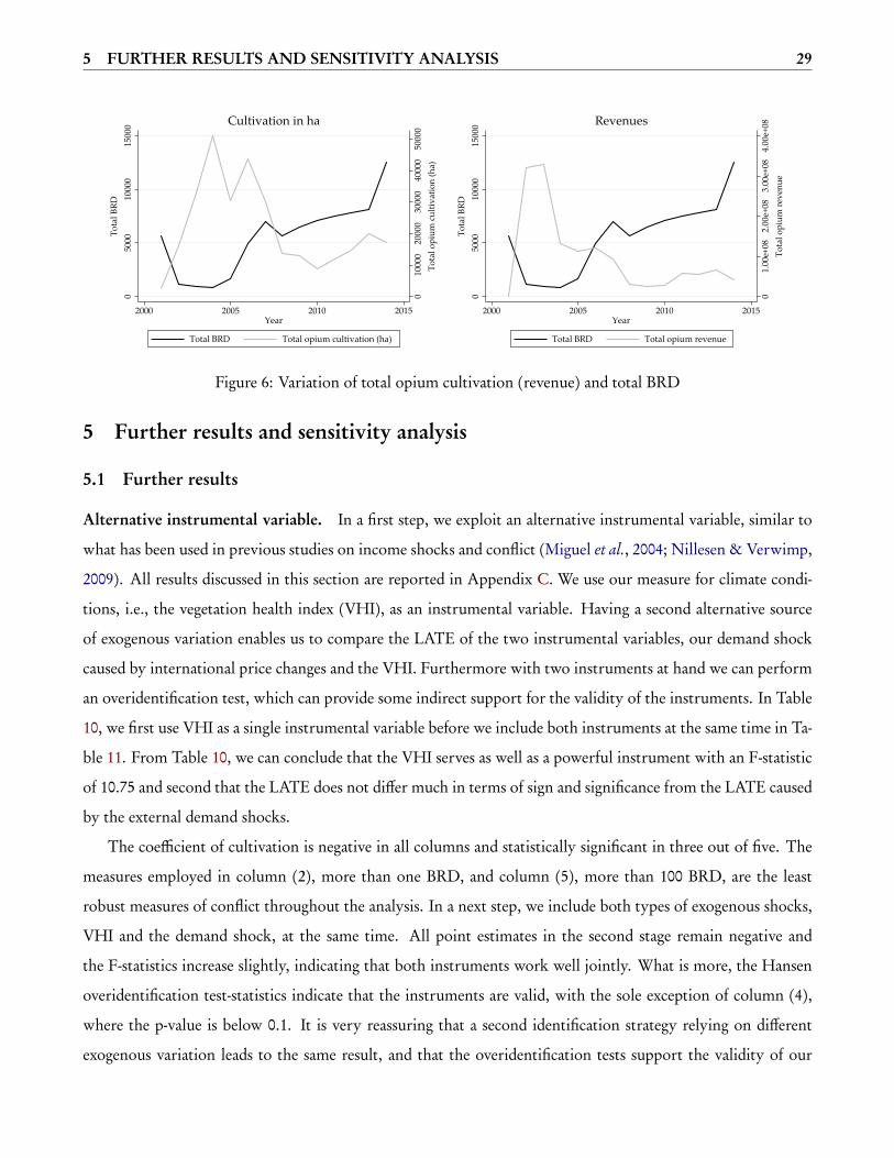
5 FURTHER RESULTS AND SENSITIVITY ANALYSIS 29
010
000
2000
030
000
4000
050
000
Tota
l opi
um c
ultiv
atio
n (h
a)
050
0010
000
1500
0To
tal B
RD
2000 2005 2010 2015Year
Total BRD Total opium cultivation (ha)
Cultivation in ha
01.
00e+
082.
00e+
083.
00e+
084.
00e+
08To
tal o
pium
reve
nue
050
0010
000
1500
0To
tal B
RD
2000 2005 2010 2015Year
Total BRD Total opium revenue
Revenues
Figure 6: Variation of total opium cultivation (revenue) and total BRD
5 Further results and sensitivity analysis
5.1 Further results
Alternative instrumental variable. In a first step, we exploit an alternative instrumental variable, similar to
what has been used in previous studies on income shocks and conflict (Miguel et al., 2004; Nillesen & Verwimp,
2009). All results discussed in this section are reported in Appendix C. We use our measure for climate condi-
tions, i.e., the vegetation health index (VHI), as an instrumental variable. Having a second alternative source
of exogenous variation enables us to compare the LATE of the two instrumental variables, our demand shock
caused by international price changes and the VHI. Furthermore with two instruments at hand we can perform
an overidentification test, which can provide some indirect support for the validity of the instruments. In Table
10, we first use VHI as a single instrumental variable before we include both instruments at the same time in Ta-
ble 11. From Table 10, we can conclude that the VHI serves as well as a powerful instrument with an F-statistic
of 10.75 and second that the LATE does not differ much in terms of sign and significance from the LATE caused
by the external demand shocks.
The coefficient of cultivation is negative in all columns and statistically significant in three out of five. The
measures employed in column (2), more than one BRD, and column (5), more than 100 BRD, are the least
robust measures of conflict throughout the analysis. In a next step, we include both types of exogenous shocks,
VHI and the demand shock, at the same time. All point estimates in the second stage remain negative and
the F-statistics increase slightly, indicating that both instruments work well jointly. What is more, the Hansen
overidentification test-statistics indicate that the instruments are valid, with the sole exception of column (4),
where the p-value is below 0.1. It is very reassuring that a second identification strategy relying on different
exogenous variation leads to the same result, and that the overidentification tests support the validity of our
5 FURTHER RESULTS AND SENSITIVITY ANALYSIS 30
instruments.
Different timing of shocks. In a second step, we consider different lag structures in our main analysis. We
do so by first including shocks in period t + 1, t , and t − 1 at the same time in Table 12, with t + 1 serving as a
falsification test. Second, we compare our main findings using shocks in t −1 to including the contemporaneous
shock separately in Table 13. Table 12 shows that the shock in t − 1, which is our preferred timing, is indeed the
shock that predominates the other two, with coefficient sizes even exceeding the ones from the main regression
(Table 2). It is reassuring to see that neither of the two other variables becomes significant, supporting the causal
order and mechanism that we hypothesize. Future international opium prices interacted with the suitability to
grow opium should not and do indeed not have a significant effect on conflict. In Table 13 we can then see that
including the contemporaneous and lagged shocks one by one results in very similar coefficients across the two
regressions. Since growing seasons differ across Afghanistan, the effects should hit farmers in different regions
and thus also people involved in processing and trafficking at different points in time.
Sample splits and outlier analysis. Third, we analyze sample splits to identify heterogeneous effects and to
control for potential outliers. In particular, we exclude all border districts from the specification in Table 14. In
that table we also report results for border districts only. Border districts could be either very different to other
districts or shocks in neighboring countries could affect border districts differently. Furthermore, we expect
a large share of trafficking occurring close to the borders. This could drive the results if international price
increases would not reach the farmers but only the traders, i.e., the ones that are closer to the final customer
along the supply chain. Our results remain very similar across the two groups of districts when we include the
strict fixed effects (Panel B).
In a similar vein, in Table 15 we drop districts in the three southern provinces Nimroz, Kandahar and
Hilmand and find our results to remain robust to this choice. These provinces are of specific interest for a
number of reasons. First, the Taliban had their origins in the southern region and is thus likely to still get most
support there. Second, these provinces are known to be the largest producers of opium. Third, simply because
of their direct connection to Pakistan, which is related to trafficking but also to the Taliban getting military
support from Pakistan. Note that even if we only included districts of these three provinces, the results remain
significantly negative and the effect size even increases (see Table 15).
As a final sample split we differentiate between districts that belonged to Taliban territory after they entered
Kabul and established the Islamic Emirate of Afghanistan in 1996 and those that did not (Dorronsoro, 2005).
Figure ?? in Appendix C shows the division of the political control in the country in fall 1996.24 Districts which
24 As discussed before, there is no time-varying data available for Taliban territory over the time and as this is of course a highlyendogenous variable, we prefer to rely on information from before our observation period.
5 FURTHER RESULTS AND SENSITIVITY ANALYSIS 31
previously belonged to the Taliban territory are likely to be still characterized by institutions set up by the
Taliban and are also likely to be more prone to a current presence of the Taliban. We hypothesized that one
channel from higher opium income to conflict could be via increased financing means of the Taliban. On the
other hand we argued that they might not have the interest in fighting where they have control and where there
is a higher opium cultivation. As it is ex ante not clear, which channel predominates the other one, it remains
an empirical question. Table 16 report the empirical results of the sample splits. Our results are not driven by
either group, with coefficients staying negative in all specifications in both sub-samples (apart from Panel A, 16
column 5). However, we do see that the districts that where under Taliban control in 1996 are characterized by
stronger effects.
Apart from these rather obvious heterogeneous groups we systematically investigate whether results are
driven by one particular province or year. Figure 7 reports the coefficients and the 90% and 95% confidence
intervals when we drop each year or each province at the time. All coefficients remain within an very narrow
band, showing that the results are not driven by outlying years or provinces.
Alternative outcome measures. To better understand who is fighting and which type of violence is used,
we now have a closer look at different types of violence and parties involved. In Table 8 we present descriptive
statistics on who is fighting. Interestingly, almost all events reported by UCDP are conflicts between the Taliban
and the Afghan government, i.e., two-sided violence involving the state. Only a minor share, not even 4%,
concerns one-sided violence by the Taliban, which does not involve the state and is directed at civilians. In our
main regressions we did not distinguish between who is fighting, but from the descriptive statistics it becomes
apparent that most results will be driven by two-sided violence between Taliban and government forces. In
Table 17 we report our baseline results for all battle-related deaths in column (1) and compare these to a more
distinct analysis of who is fighting. In column (2) where we define our outcome as all casualties that occurred
from violence perpetrated by the Taliban against civilians, we see a much smaller but still significantly negative
effect in our preferred specification (Panel B). Note that this classification does not include many cases, as less
then 4% of all events fall into this definition. This indicates that the conflict-reducing effect is also leading to
less violence started by the rebels. Columns (3) to (5) cover violent events between Taliban and government.
In all specifications, irrespective of whether we look at total casualties or only casualties at one side, we see the
negative effect persisting. This exercise provides evidence for a very robust conflict-reducing effects of opium
income on all types of violence that persist throughout our observation period.
As another alternative outcome, we consider heterogeneous effects on onset and ending of conflict events.
So far, we have not addressed dynamics. Though, as conflict is a persistent phenomenon, we also investigate
the effects from a more dynamic perspective. While the literature at the micro-level mainly ignores the role of
5 FURTHER RESULTS AND SENSITIVITY ANALYSIS 32
persistence and state-dependence, a new trend in the macro-literature stresses this role, theoretically (Acemoglu
& Wolitzky 2014) and empirically (Bluhm et al. 2016).25 In a first step, we follow the micro-level literature
in measuring the effects in separate models. Results are presented in Table 18. For comparison to the results
with our main outcome variable, conflict incidence, we plot conditional logit results for conflict incidence in
Panel A. Panel B then reports the results for onset and Panel C for ending of a conflict. Onset and ending
are defined as binary indicators, which take a value of one conditional on the previous state of conflict. More
precisely, we define conflict onset as the incidence of a conflict in a district, where there was no conflict in the
previous year (Con f l ic ti,t = 1|Con f l ic ti,t−1 = 0). Years of ongoing conflict are set to missing. In analogy,
a conflict ending is defined when conflict persisted in the previous year but not anymore in the current year
(Con f l ic ti,t = 0|Con f l ic ti,t−1 = 1).26 Panel A supports our main finding using linear probability models,
as we see that our main results are robust to using a non-linear model. In Panel B we find that an opium
shock reduces the likelihood of a conflict onset for conflicts measures up to a threshold of 25 BRD. For conflict
ending, we only find a significantly positive effect in column (1). This result indicates that a positive income
shock, which increases opium cultivation, raises the likelihood of a conflict - measured in the strictest sense - to
end. In a second step, we account for conflict dynamics by including the lagged dependent variable. This again,
does not change our main results. The opium shock remains negative (in Panel A and B) and in all columns
statistically significant in the specifications with the stricter fixed effects (Panel B). Results are reported in Table
19.
Lastly, we alter the dependent variable by using ACLED conflict data. We create three different measures
from the ACLED dataset. Precisely, we take the logarithm of the number of all events reported, the subset of
violent events, and the subset of violent events against civilians. We report results for the most stringent fixed
effects specification in Table 20 in Panel A-C. Panel A and B report results with standard errors clustered at
the district-level (Panel A) and at the province-level (Panel B). In Panel C we exchange the opium suitability
measure with the weighted suitability measure. Despite having a much shorter period of observation our results
still point to the conflict-reducing effect of positive income shocks. Results are, however, less strong in Panel
B where standard errors are clustered at the province-level. Though, the general picture remains very similar
when we use ACLED rather than UCDP (GED) conflict data.
Taken together, we have seen that our results do not depend on the specific income shock we employ. We
find very similar results when exploiting climate conditions to induce exogenous variation in opium cultivation.
25 Berman & Couttenier (2015) for instance argue that persistence is very low at their level of analysis (a cell equivalent to 55×55kilometers at the equator) compared to country-level data. Consequently, they do not include the lagged dependent and ratherestimate separate models for onset and ending. We report transition probabilities of the different conflict intensities from peace towar in Table 9.
26 We also set the ending variable missing for observations which have been at peace in the previous year and remained in peace in thecurrent year, following the standards in the literature.
5 FURTHER RESULTS AND SENSITIVITY ANALYSIS 33
This is a reassuring finding that we do not capture a very specific LATE, which might not be representative.
What is more, we find the effect throughout the country. When we exclude regions of particular interest or
regions likely to be outlying, results still show a conflict-reducing effect of higher opium income. We also find
evidence for the effect to remain irrespective of how the outcome variable is defined, i.e., for different types of
fighting, conflict onset and ending, and conflict measured by events (ACLED) rather than by the number of
BRD.
5.2 Sensitivity analysis
We now investigate the sensitivity of our results to different specification choices even further. All results
discussed in this section are reported in Appendix D. First, we adjust our variable of main interest, the external
income shock. Second we run several robustness checks by using different choices on how we cluster the
standard errors. Third we include further control variables and trends.
Modifications of the treatment variable. As discussed, we replace the average international price index (co-
caine, amphetamines and ecstasy) with the international cocaine price in Table 21 and find our results to be
unaffected by this choice. We also replace this index with the deviation of the international prices from their
long-term mean in Table 22. This is a first attempt to rule out that our results are driven by the long-term
negative trend in all international drug prices as seen in Figure 3. The effect of the opium shock still remains
significantly negative for columns (1) to (4).27 Next, we normalize the prices of the three drugs before we take
the average and then proceed as before. This could matter as ecstasy and amphetamines are cheaper than cocaine,
so that changes in the more expensive drug could dominate changes in the index. The results using normalized
prices in Table 23 show that this does not affect our estimations.
What is more, Table 24 replaces the international exogenous prices with the local Afghan price for opium in
constant 2010 EU/kg, measured at the farm-gate-level. We are aware that this introduces endogeneity, but also
that the interaction term between an endogenous variable (the Afghan price) and an exogenous variable (the
suitability) could still produce causal estimates under some assumptions (see Dreher et al., 2016). Moreover, the
Afghan price is the best proxy for the prices supplier in Afghanistan receive, whereas the world market price is
many times higher. We make two main observations. First we note that the sign of the effects remains negative
and significant in most specifications. Second, the pattern that the more conservative fixed effects specifications
lead to more negative estimates is repeated (with the exception of column 2). This is in line with our previous
findings that on average omitted variable bias tends to be positive.
Besides adjusting the price variable we also try an alternative opium suitability index. This alternative
27 Specifically, we use the mean over the entire observation period. Due to data restrictions we cannot calculate longer-term means.
5 FURTHER RESULTS AND SENSITIVITY ANALYSIS 34
weights the suitabilities of opium and wheat by the (lagged) population distribution within the districts. As
can be seen in Table 25, the results for the opium shock remain virtually identical for all specifications. The
main difference is that the wheat shock is now negative in most specifications as well, also more in line with an
opportunity cost based explanation of resources and conflict in Afghanistan.
Standard errors. In a next step, we use different choices on how to cluster the standard errors. In the baseline
models we used the district-level, allowing for serial correlation over time within a district. Table 26 clusters
at the province-level in Panel A allowing for spatial correlation within a province over time. In Panel B and C
we use two-way clustering , i.e. district and year clusters and province and year clusters, respectively (Cameron
et al., 2011). The number of clusters using the province-level might be too small using the regular formula for
clustered standard errors, which can lead to the over- or under-rejection of the null hypothesis (Cameron &
Miller, 2015). Accordingly, we also use the wild-cluster bootstrap method with the null imposed with 1000
replications and Webb’s weights (Webb, 2013), which has been shown to provide valid inference even for few
clusters. Figure 8 plot the distribution of the bootstrap estimates. The null hypothesis of no effect if is rejected
in all cases (except for war) at least at the 5%-level. This is apparent in the graphs by the fact that the 95%-
confidence intervals do not include zero.
Further covariates and trends. Finally, we include further covariates and trends. So far, we have only in-
cluded the wheat shock and different fixed effects in the regressions and no other covariates. In Table 27 (Panel
A) we add the baseline set of pre-determined covariates as luminosity and population as well as an exogenous
measure of droughts, the VHI. In further specifications (Panel B), we also allow for time-varying effects of
time-invariant control variables. The set of time-invariant covariates includes ruggedness, heroin/morphine lab,
major/sub opium markets, main/secondary roads, military camps, proximity to Kabul, unofficial border cross-
ings, presence of Pashtuns, Taliban territory in 1996. One way to model that is by adding interactions between
these variables and a time trend. Another more flexible way is to interact the time invariant control variables
with year dummies (Panel C). In both panels, our main treatment variable remains significant with p-values be-
low at least 0.1 for all conflict proxies. Furthermore, in analogy to Christian & Barrett (2017) we include linear
and nonlinear suitability specific trends. We classify the suitability to grow opium into quartiles and include a
linear and a nonlinear quartile specific trend in our main regression analysis. Our results are not affected by this
change.
6 CONCLUSION 35
6 Conclusion
This paper identifies the causal effect of opium cultivation on conflict in Afghanistan, with opium being an
illegal renewable resource that is often linked to conflict and instability. To induce exogenous variation in
opium cultivation we make use of external demand shocks that affect income and conflict through changes in
opium cultivation. Our identification strategy exploits variation in international prices of alternative drugs as
well as in land suitability for growing opium. The interaction term of the two variables thus combines temporal
and spatial variation. We apply this to a reduced form equation and an instrumental variable approach in a panel
data setting at the Afghan district-level over the 2002 to 2014 period.
Many papers have analyzed the relationship between resources and conflict, but yet we are far from under-
standing the micro-foundations. In particular, the role that features of resources and market structures play are
highly under-researched. Our findings thus augment the literature on the determinants of conflict and more
specifically on the resource-conflict nexus in important ways. First, we suggest a new identification strategy
to identify the causal direction of the link between illicit economies and violence. With notable exceptions
(Angrist & Kugler 2008; Mejıa & Restrepo 2015) this has not been addressed in the literature. Second, by
investigating the reasons for heterogeneous effects across different types of resources and across different charac-
teristics of a country or sub-national area. More precisely, we differentiate between resources according to their
labor intensity and legality and we compare the effects across districts which differ according to the extent of
government presence and share of value-added along the supply chain of opium. This helps to better understand
the mechanisms behind the effect of resources on conflict. Third, we augment the literature by providing new
insights on the geography of conflict in Afghanistan, which also provides important political insights.
We find that the external price shock works well as an instrument for actual opium cultivation. Our findings
at the district-level show that international price changes in other drugs robustly affect opium cultivation and
local opium prices, irrespective of the empirical model and the exact definition of the dependent variable. Higher
opium profitability and cultivation leads to a lower incidence of conflict. All models indicate that the coefficient
of the income shock is biased upwards in OLS regressions. This is visible by the fact that the point estimates
become more negative when adding a stricter set of fixed effects and when replacing the endogenous direct
opium income shocks with the plausibly exogenous income shocks. The results are further backed by using a
different instrumentation strategy relying on exogenous weather changes.
What is more, we find a number of heterogeneous effects of the external income shock on the risk of conflict.
The conflict-reducing effect is stronger in districts in which opium is not only grown in its raw form, but also
processed and traded. We argue that this is due to the fact that such districts can capture a larger share of
the value-added along the supply chain. In contrast, the effect is smaller in districts where Western casualties
6 CONCLUSION 36
occurred or where government institutions are likely to be more present. There are several plausible reasons
for this. Money raised by drug production might be used to also finance attacks on government or Western
ISAF forces. At the same time these districts are likely to be characterized by a stronger presence of the state
and police force, which could lead to increased opium eradication efforts or less possibilities to grow and trade
opium.
Our results are in line with Berman & Couttenier (2015) who find evidence for the opportunity cost hy-
pothesis. We further add support to Dube & Vargas (2013)’s seminal study, by showing that the importance
of labor intensity in determining the effect of a resource boom is not solely restricted to Colombia. Opium is
the most labor-intensive crop compared to alternative crops in Afghanistan, so that shifting away from opium
production would come along with less labor and thus reduced opportunity costs of fighting. On the other
hand, our results are at first sight at odds with the findings in Angrist & Kugler (2008) and Mejıa & Restrepo
(2015), who find that an increase in the estimated profitability of cocaine leads to more homicides in Colombia.
As Mejıa & Restrepo (2015) identify the opposite effect for legal crops, they argue that the conflict-increasing
effect of cocaine is due to its (il-)legal status. Our findings strongly indicate that it is not about the illegality of
a crop per se, but rather that the relative labor intensity of alternative crops or income sources and local market
structures are crucial.
Our results on heterogeneous effects highlight that it is important not to treat the resource-conflict rela-
tionship as a black box, but to consider the individual actors involved in market transactions and conflict. The
available data does not allow to distinguish whether opportunity costs considerations are more important at the
level of small-scale farmers or local elites. Most likely, both groups benefit from higher profitability and have
less incentives to engage in fighting. Still, our results suggest that there might be a trade-off for the Taliban. If
government presence is estimated to be stronger in a district, the revenues also seem to support anti-government
activities. Accordingly, our results do by no means suggest that revenues from drug production procuring to
a dangerous group like the Taliban are not a problem. What they show is that on average, the effect of more
opium revenues leads to less conflict. Generally, opium is too important for large shares of the Afghan society
for simple prohibition to work. It thus becomes clear that simplistic attempts to fight opium production with
large eradication programs will have unintended consequences, if there are no available alternatives that can
employ a comparable amount of labor.
REFERENCES 37
References
Acemoglu, Daron, & Wolitzky, Alexander. 2014. Cycles of conflict: An economic model. The American
Economic Review, 104(4), 1350–1367. 32
Angrist, Joshua D., & Kugler, Adriana D. 2008. Rural Windfall or a New Resource Curse? Coca, Income, and
Civil Conflict in Colombia. The Review of Economics and Statistics, 90(2), 191–215. 2, 7, 35, 36
Bazzi, Samuel, & Blattman, Christopher. 2014. Economic Shocks and Conflict: Evidence from Commodity
Prices. American Economic Journal: Macroeconomics, 6(4), 1–38. 2
Berman, Eli, Felter, Joseph H, Shapiro, Jacob N, & Callen, Michael. 2010. Do Working Men Rebel? Journal of
Conflict Resolution, 55(4), 496–528. 23
Berman, Nicolas, & Couttenier, Mathieu. 2015. External shocks, Internal Shots: The Geography of Civil
Conflicts. Review of Economics and Statistics, 97(4), 758–776. 2, 8, 12, 13, 32, 36
Berman, Nicolas, Couttenier, Mathieu, & Rohner, Dominic. 2017. This Mine is Mine! How Minerals Fuel
Conflicts in Africa. American Economic Review, 107(6), 1564–1610. 2
Blattman, Christopher, & Miguel, Edward. 2010. Civil war. Journal of Economic literature, 48(1), 3–57. 2
Bluhm, Richard, Gassebner, Martin, Langlotz, Sarah, & Schaudt, Paul. 2016. Fueling Conflict?(De) Escalation
and Bilateral Aid. 32
Bove, Vincenzo, & Elia, Leandro. 2013. Drugs and violence in Afghanistan: A panel VAR with unobserved
common factor analysis. Defence and Peace Economics, 24(6), 535–554. 3, 4, 5
Brückner, Markus, & Ciccone, Antonio. 2010. International Commodity Prices, Growth and the Outbreak of
Civil War in Sub-Saharan Africa. The Economic Journal, 120(544), 519–534. 2
Cameron, A. Colin, & Miller, Douglas L. 2015. A Practitioners Guide to Cluster-Robust Inference. Journal of
Human Resources, 50(2), 317–372. 34
Cameron, A. Colin, Gelbach, Jonah B., & Miller, Douglas L. 2011. Robust Inference with Multiway Clustering.
Journal of Business & Economic Statistics, 29(2), 238–249. 34
Caulkins, Jonathan Paul, Kleiman, Mark, & Kulick, Jonathan D. 2010. Drug Production and Trafficking, Coun-
terdrug Policies, and Security and Governance in Afghanistan. New York University Center on International
Cooperation. 12
REFERENCES 38
Chabot, Philippe, & Dorosh, Paul A. 2007. Wheat markets, Food Aid and Food Security in Afghanistan. Food
Policy, 32(3), 334–353. 20
Christian, Paul, & Barrett, Christopher. 2017. Revisiting the Effect of Food Aid on Conflict: A Methodological
Caution. 34
Collier, Paul, & Hoeffler, Anke. 2004. Greed and Grievance in Civil War. Oxford economic papers, 56(4),
563–595. 2, 4
Croicu, Mihai, & Sundberg, Ralph. 2015. UCDP GED Codebook version 4.0. Department of Peace and Conflict
Research, Uppsala University. 8, 1
De La Sierra, Raúl Sánchez, et al. 2015. On the origin of states: Stationary bandits and taxation in eastern congo.
Tech. rept. Households in Conflict Network. 5
Dell, Melissa. 2015. Trafficking Networks and the Mexican Drug War. The American Economic Review, 105(6),
1738–1779. 2
Dorronsoro, Gilles. 2005. Revolution Unending: Afghanistan, 1979 to the Present. Columbia University Press.
23, 30, 4
Dreher, Axel, & Langlotz, Sarah. 2017. Aid and growth. New evidence using an excludable instrument. Heidel-
berg University Discussion Paper No. 635. 3
Dreher, Axel, Eichenauer, Vera Z., & Gehring, Kai. 2016. Geopolitics, Aid, and Growth: The Impact of UN
Security Council Membership on the Effectiveness of Aid. The World Bank Economic Review. 33
Dube, Oeindrila, & Vargas, Juan F. 2013. Commodity Price Shocks and Civil Conflict: Evidence from Colom-
bia. The Review of Economic Studies, 80(4), 1384–1421. 1, 2, 4, 6, 23, 36
EMCDDA. 2016. European Drug Report - Trends and Developments. Luxembourg: Publications Office of the
European Union, 2016. 14
Fearon, James D. 2005. Primary Commodity Exports and Civil War. Journal of conflict Resolution, 49(4),
483–507. 2
Fearon, James D, & Laitin, David D. 2003. Ethnicity, insurgency, and civil war. American political science
review, 97(01), 75–90. 2
REFERENCES 39
Felbab-Brown, Vanda. 2013. Counterinsurgency, Counternarcotics, and Illicit Economies in Afghanistan:
Lessons for State-Building. MM Jacqueline Brewer, Convergence: Illicit Networks and National Security in the
Age of Globalization, 189–212. 3, 6
Gehring, Kai, & Schneider, Stephan. 2016. Regional Resources and Democratic Secessionism. ETH and Univer-
sity of Zurich CIS Working Paper Series No. 90. 2
Giustozzi, Antonio. 2009. Empires of Mud: the Neo-Taliban Insurgency in Afghanistan 2002-2007. Columbia
University Press. 13, 24, 4
Grossman, Herschell I. 1991. A general equilibrium model of insurrections. The American Economic Review,
912–921. 4
Harari, Mariaflavia, & La Ferrara, Eliana. 2013. Conflict, Climate and Cells: A Disaggregated Analysis. CEPR
Discussion Paper, February 2014(DP9277), 1–64. 11
Henderson, J Vernon, Storeygard, Adam, & Weil, David N. 2012. Measuring Economic Growth from Outer
Space. American Economic Review, 102(2), 994–1028. 11
Hijmans, Robert J., Guarino, Luigi, Cruz, Mariana, & Rojas, Edwin. 2001. Computer tools for spatial analysis
of plant genetic resources data: 1. DIVA-GIS. Plant Genetic Resources Newsletter, 127, 15–19. 9, 3
Hirshleifer, Jack. 1988. The analytics of continuing conflict. Synthese, 76(2), 201–233. 4
Hirshleifer, Jack. 1989. Conflict and rent-seeking success functions: Ratio vs. difference models of relative
success. Public choice, 63(2), 101–112. 4
Hirshleifer, Jack. 1995. Anarchy and its breakdown. Journal of Political Economy, 26–52. 4
Humphreys, Macartan. 2005. Natural resources, conflict, and conflict resolution: Uncovering the mechanisms.
Journal of Conflict Resolution, 49(4), 508–37. 2
Kienberger, Stefan, Spiekermann, Raphael, Tiede, Dirk, Zeiler, Irmgard, & Bussink, Coen. 2016. Spatial Risk
Assessment of Opium Poppy Cultivation in Afghanistan: Integrating Environmental and Socio-Economic
Drivers. International Journal of Digital Earth, November 2016, 1–18. 4, 9, 10, 3
Kreutzmann, Hermann. 2007. Afghanistan and the Opium World Market: Poppy Production and Trade. Ira-
nian Studies, 40(5), 605–621. 24, 25
La Ferrara, Eliana, & Guidolin, Massimo. 2007. Diamonds are forever, wars are not: Is conflict bad for private
firms? American Economic Review, 97(5), 1978–1993. 2
REFERENCES 40
Leri, Francesco, Bruneau, Julie, & Stewart, Jane. 2003. Understanding polydrug use: review of heroin and
cocaine co-use. Addiction, 98, 7–22. 14
Lind, Jo Thori, Moene, Karl Ove, & Willumsen, Fredrik. 2014. Opium For the Masses? Conflict-Induced
Narcotics Production in Afghanistan. Review of Economics and Statistics, 96(5), 949–966. 3, 4, 23
Lujala, Paivi. 2009. Deadly Combat over Natural Resources: Gems, Petroleum, Drugs, and the Severity of
Armed Civil Conflict. Journal of Conflict Resolution, 53(1), 50–71. 2
Lyall, Jason, Blair, Graeme, & Imai, Kosuke. 2013. Explaining Support for Combatants During Wartime: A
Survey Experiment in Afghanistan. American Political Science Review, 107(04), 679–705. 2
Mansfield, David, & Fishstein, Paul. 2016. Time to Move on: Developing an Informed Development Response to
Opium Poppy Cultivation in Afghanistan. Tech. rept. Afghanistan Research and Evaluation Unit. 3, 4, 5, 12,
20
Mejıa, Daniel, & Restrepo, Pascual. 2015. Bushes and Bullets: Illegal Cocaine Markets and Violence in Colom-
bia. mimeo. 1, 2, 7, 21, 23, 35, 36
Mejía, Daniel, Restrepo, Pascual, & Rozo, Sandra V. 2015. On the effects of enforcement on illegal markets:
evidence from a quasi-experiment in Colombia. The World Bank Economic Review, l–051. 6
Michalopoulos, Stelios, & Papaioannou, Elias. 2013. Pre-colonial Ethnic Institutions and Contemporary African
Development. Econometrica, 81(1), 113–152. 11
Michalopoulos, Stelios, & Papaioannou, Elias. 2014. National Institutions and Subnational Development in
Africa. The Quarterly Journal of Economics, 129(1), 151–213. 10
Miguel, Edward, Satyanath, Shanker, & Sergenti, Ernest. 2004. Economic Shocks and Civil Conflict: An
Instrumental Variables Approach. Journal of political Economy, 112(4), 725–753. 2, 29
Morelli, Massimo, & Rohner, Dominic. 2015. Resource Concentration and Civil Wars. Journal of Development
Economics. 2
Nillesen, Eleonora E, & Verwimp, Philip. 2009. Grievance, Commodity Prices and Rainfall: A Village-Level
Analysis of Rebel Recruitment in Burundi. HiCNWorking Paper, April 2009(58), 1–21. 29
Nunn, Nathan, & Puga, Diego. 2012. Ruggedness: The Blessing of Bad Geography in Africa. Review of
Economics and Statistics, 94(1), 20–36. 3
REFERENCES 41
Nunn, Nathan, & Qian, Nancy. 2014. US Food Aid and Civil Conflict. American Economic Review, 104(6),
1630–66. 3
Peters, Gretchen. 2009. How Opium Profits the Taliban. Vol. 31. United States Institute of Peace Washington
DC:. 5
Raleigh, Clionadh, Linke, Andrew, Hegre, Havard, & Karlsen, Joakim. 2010. Introducing ACLED-Armed
Conflict Location and Event Data. Journal of Peace Research, 47(5), 651–660. 2
Ross, Michael. 2004. How Do Natural Resources Influence Civil War? Evidence From 13 Cases. International
Organization, 58(1), 35–68. 2
Rubin, Barnett R, & Sherman, Jack. 2008. Counter-narcotics to stabilize Afghanistan: The false promise of crop
eradication. UNDP. 6
Sexton, Renard. 2016. Aid as a Tool against Insurgency: Evidence from Contested and Controlled Territory in
Afghanistan. The American Political Science Review, 110(4), 731. 2
Staiger, Douglas O, & Stock, James H. 1997. Instrumental variables regression with weak instruments. Econo-
metrica, 65(3), 557–586. 21
Sundberg, Ralph, & Melander, Erik. 2013. Introducing the UCDP Georeferenced Event Datas. Journal of Peace
Research, 50(4), 523–532. 8, 1
UNODC. 2004. Farmers’ intentions survey 2003/2004. UNODC Report. 5
UNODC. 2005. Afghanistan Opium Survey 2005. Vienna: United Nations, Office on Drugs and Crime. 4
UNODC. 2009. Afghanistan Opium Survey 2009. Vienna: United Nations, Office on Drugs and Crime. 3
UNODC. 2013a. Afghanistan Opium Survey 2013. Vienna: United Nations, Office on Drugs and Crime. 4, 5
UNODC. 2013b. World Drug Report 2013. United Nations Publication Sales. 14, 16
UNODC. 2015. Afghanistan Opium Survey 2015. Vienna: United Nations, Office on Drugs and Crime. 12
UNODC. 2016. Afghanistan Opium Survey 2016. Vienna: United Nations, Office on Drugs and Crime. 3
Webb, Matthew D. 2013. Reworking Wild Bootstrap Based Inference for Clustered Errors. Queen’s Economics
Department Working Paper 1315. 34
Weidmann, Nils B., Rød, Jan Ketil, & Cederman, Lars-Erik. 2010. Representing Ethnic Groups in Space: A
New Dataset. Journal of Peace Research, 47(4), 491–499. 1, 24
A DEFINITION OF THE VARIABLES 1
Appendix
A Definition of the Variables
Battle Related Deaths (BRD): The best (most likely) estimate of total fatalities resulting from an event, with
an event being defined as “[an] incident where armed force was by an organized actor against another organized
actor, or against civilians, resulting in at least 1 direct death at a specific location and a specific date.” A direct
death is defined as “a death relating to either combat between warring parties or violence against civilians.” Note
that UCDP/GED only includes BRD of events that belong to a dyad (“two conflicting primary parties or party
killing unarmed civilians”) that reached in total at least 25 BRD within a year. If the dyad generated events with
less then 25 BRD in the previous or subsequent years, they are still counted if the dyad had reached the 25 BRD
threshold in another year. We construct a continuous measure (log of BRD) and binary outcomes from all BRD
of any party or any type of violence (state-based, non-state or one-sided violence). Since UCDP/GED provides
information on the parties and the type of violence we also construct specific outcome measures according to
those categories. From UCDP/GED (Sundberg & Melander, 2013; Croicu & Sundberg, 2015).
Vegetation Health Index (VHI): We use the Vegetation Health Index (VHI) of FAO (van Hoolst et al.
2016). VHI is a composite index joining the Vegetation Condition Index (VCI) and the Temperature Condition
Index (TCI, Kogan 1995). Low values of VHI represent drought conditions. This is a combination of low
values of the observed VCI (relatively low vegetation) and higher values of the TCI (relatively warm weather).
For details see van Hoolst et al. (2016). The VHI is calculated from data of Advanced Very High Resolution
Radiometer (AVHRR) sensors on board the National Oceanic and Atmospheric Administration (NOAA) and
Meteorological Operational Satellite (METOP) satellites.
Consumer Price Index (CPI): (2010 = 100). From the Organization for Economic Cooperation and
Development (OECD, 2016) for the Euro area (19 countries) and from WDI (2016) for remaining countries.
Drug Prices (International): The data are average prices per gram in constant (2010) EU across all available
countries in Europe. We use data on different drugs: amphetamines, cocaine, ecstasy, heroin (white and brown).
To construct the average price of alternative drugs we use a mean of the three upper drugs amphetamines,
cocaine, and ecstasy. From European Drug Report 2016, the European Monitoring Centre for Drugs and Drug
Addiction (EMCDDA, 2016).
Ethnic groups: We have used the GIS-coordinates of all ethnic groups in the “georeferencing of ethnic
groups” (GREG) dataset Weidmann et al. (2010). It relies on maps from the classical “Soviet Atlas Narodov
Mira” from 1964, and is very extensively used for the construction of ethnolinguistic fractionalization (ELF)
indices. GREG is a georeferenced dataset containing the coordinates of the group boundaries of 1120 ethnic
A DEFINITION OF THE VARIABLES 2
groups. One advantage and disadvantage of the data is that it is capturing group locations in the 1960s. This is
an advantage as it ensures that the boundaries are not endogenous to changes during our period of observation.
It is partly a disadvantage if groups and countries changed over time. In Afghanistan, the country boundary
did not change. Ethnic group populations certainly change to some degree over time, so that all variables more
precisely capture the historic homelands of ethnic groups rather than the current settlement areas. Our variable
(no) Pashtuns is coded in the following way. The GREG polygons can contain more than one ethnic group.
Our binary indicator takes on the value one if Pashtuns are not present to any degree in a district, regardless of
whether they were the majority group. The idea behind this is that the Taleban are initially a Pashtun group
(although not exclusively anymore), so that Pashtun presence could make it easier to establish a presence of the
Taliban in a district.
Events: An event is defined according to those within an UCDP/PRIO armed conflict. ACLED differenti-
ates between violent and nonviolent and between different types of violence.We define an event to be nonviolent
if it belongs to one of the types: "Non-violent rebel activity", "Riots/Protests", or “Non-violent activity by a
conflict actor". Violent events are those that involve a battle between government and rebels or involve violence
against civilians. We construct the variable “All Events”, which includes both types of events and a variable
“Violent Events” referring to the latter category only. Finally we also construct a variable that included only
“Violence against Civilians”. For all event variables we take the logarithm. From ACLED (Raleigh et al., 2010).
Inflation, GDP deflator: (2010 = 100). GDP deflator for the US with 2010 as the base year. From World
Development Indicators - The World Bank (2016).
Insecurity/violence shock: The share of sampled households that have experienced a shock due to inse-
curity/ violence according to the NRVA survey. From the National Risk and Vulnerability Assessment (2005,
2007/08, 2011/12).
Luminosity: Proxy for GDP and development. The files are cloud-free composites made using all the
available archived DMSP-OLS smooth resolution data for calendar years. The products are 30 arc second grids,
spanning -180 to 180 degrees longitude and -65 to 75 degrees latitude. A number of constraints are used to select
the highest quality data for entry into the composites: Data are from the center half of the 3000 km wide OLS
swaths. Lights in the center half have better geolocation, are smaller, and have more consistent radiometry.
Sunlit data are excluded based on the solar elevation angle. Glare is excluded based on solar elevation angle.
Moonlit data are excluded based on a calculation of lunar illuminance. Observations with clouds are excluded
based on clouds identified with the OLS thermal band data and NCEP surface temperature grids. Lighting
features from the aurora have been excluded in the northern hemisphere on an orbit-by-orbit manner using
visual inspection. From Version 4 DMSP-OLS nighttime lights time series, National Oceanic and Atmospheric
Administration-National Geophysical Data Center (NOAA/NGDC), 2013.
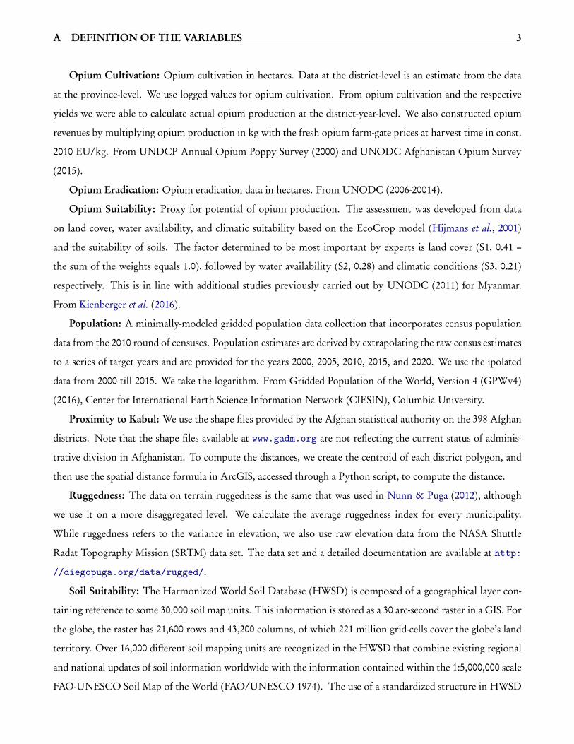
A DEFINITION OF THE VARIABLES 3
Opium Cultivation: Opium cultivation in hectares. Data at the district-level is an estimate from the data
at the province-level. We use logged values for opium cultivation. From opium cultivation and the respective
yields we were able to calculate actual opium production at the district-year-level. We also constructed opium
revenues by multiplying opium production in kg with the fresh opium farm-gate prices at harvest time in const.
2010 EU/kg. From UNDCP Annual Opium Poppy Survey (2000) and UNODC Afghanistan Opium Survey
(2015).
Opium Eradication: Opium eradication data in hectares. From UNODC (2006-20014).
Opium Suitability: Proxy for potential of opium production. The assessment was developed from data
on land cover, water availability, and climatic suitability based on the EcoCrop model (Hijmans et al., 2001)
and the suitability of soils. The factor determined to be most important by experts is land cover (S1, 0.41 –
the sum of the weights equals 1.0), followed by water availability (S2, 0.28) and climatic conditions (S3, 0.21)
respectively. This is in line with additional studies previously carried out by UNODC (2011) for Myanmar.
From Kienberger et al. (2016).
Population: A minimally-modeled gridded population data collection that incorporates census population
data from the 2010 round of censuses. Population estimates are derived by extrapolating the raw census estimates
to a series of target years and are provided for the years 2000, 2005, 2010, 2015, and 2020. We use the ipolated
data from 2000 till 2015. We take the logarithm. From Gridded Population of the World, Version 4 (GPWv4)
(2016), Center for International Earth Science Information Network (CIESIN), Columbia University.
Proximity to Kabul: We use the shape files provided by the Afghan statistical authority on the 398 Afghan
districts. Note that the shape files available at www.gadm.org are not reflecting the current status of adminis-
trative division in Afghanistan. To compute the distances, we create the centroid of each district polygon, and
then use the spatial distance formula in ArcGIS, accessed through a Python script, to compute the distance.
Ruggedness: The data on terrain ruggedness is the same that was used in Nunn & Puga (2012), although
we use it on a more disaggregated level. We calculate the average ruggedness index for every municipality.
While ruggedness refers to the variance in elevation, we also use raw elevation data from the NASA Shuttle
Radat Topography Mission (SRTM) data set. The data set and a detailed documentation are available at http:
//diegopuga.org/data/rugged/.
Soil Suitability: The Harmonized World Soil Database (HWSD) is composed of a geographical layer con-
taining reference to some 30,000 soil map units. This information is stored as a 30 arc-second raster in a GIS. For
the globe, the raster has 21,600 rows and 43,200 columns, of which 221 million grid-cells cover the globe’s land
territory. Over 16,000 different soil mapping units are recognized in the HWSD that combine existing regional
and national updates of soil information worldwide with the information contained within the 1:5,000,000 scale
FAO-UNESCO Soil Map of the World (FAO/UNESCO 1974). The use of a standardized structure in HWSD
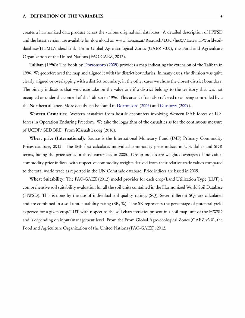
A DEFINITION OF THE VARIABLES 4
creates a harmonized data product across the various original soil databases. A detailed description of HWSD
and the latest version are available for download at: www.iiasa.ac.at/Research/LUC/luc07/External-World-soil-
database/HTML/index.html. From Global Agro-ecological Zones (GAEZ v3.0), the Food and Agriculture
Organization of the United Nations (FAO-GAEZ, 2012).
Taliban (1996): The book by Dorronsoro (2005) provides a map indicating the extension of the Taliban in
1996. We georeferenced the map and aligned it with the district boundaries. In many cases, the division was quite
clearly aligned or overlapping with a district boundary, in the other cases we chose the closest district boundary.
The binary indicators that we create take on the value one if a district belongs to the territory that was not
occupied or under the control of the Taliban in 1996. This area is often also referred to as being controlled by a
the Northern alliance. More details can be found in Dorronsoro (2005) and Giustozzi (2009).
Western Casualties: Western casualties from hostile encounters involving Western ISAF forces or U.S.
forces in Operation Enduring Freedom. We take the logarithm of the casualties as for the continuous measure
of UCDP/GED BRD. From iCasualties.org (2016).
Wheat price (International): Source is the International Monetary Fund (IMF) Primary Commodity
Prices database, 2013. The IMF first calculates individual commodity price indices in U.S. dollar and SDR
terms, basing the price series in those currencies in 2005. Group indices are weighted averages of individual
commodity price indices, with respective commodity weights derived from their relative trade values compared
to the total world trade as reported in the UN Comtrade database. Price indices are based in 2005.
Wheat Suitability: The FAO-GAEZ (2012) model provides for each crop/Land Utilization Type (LUT) a
comprehensive soil suitability evaluation for all the soil units contained in the Harmonized World Soil Database
(HWSD). This is done by the use of individual soil quality ratings (SQ). Seven different SQs are calculated
and are combined in a soil unit suitability rating (SR, %). The SR represents the percentage of potential yield
expected for a given crop/LUT with respect to the soil characteristics present in a soil map unit of the HWSD
and is depending on input/management level. From the From Global Agro-ecological Zones (GAEZ v3.0), the
Food and Agriculture Organization of the United Nations (FAO-GAEZ), 2012.
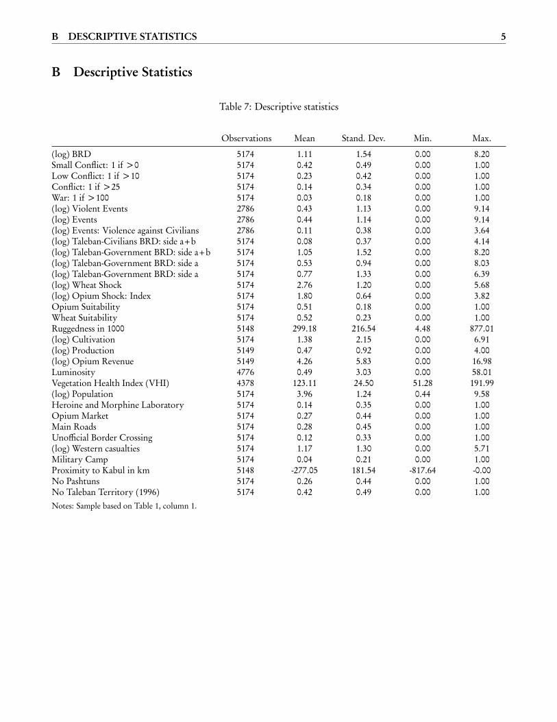
B DESCRIPTIVE STATISTICS 5
B Descriptive Statistics
Table 7: Descriptive statistics
Observations Mean Stand. Dev. Min. Max.
(log) BRD 5174 1.11 1.54 0.00 8.20Small Conflict: 1 if >0 5174 0.42 0.49 0.00 1.00Low Conflict: 1 if >10 5174 0.23 0.42 0.00 1.00Conflict: 1 if >25 5174 0.14 0.34 0.00 1.00War: 1 if >100 5174 0.03 0.18 0.00 1.00(log) Violent Events 2786 0.43 1.13 0.00 9.14(log) Events 2786 0.44 1.14 0.00 9.14(log) Events: Violence against Civilians 2786 0.11 0.38 0.00 3.64(log) Taleban-Civilians BRD: side a+b 5174 0.08 0.37 0.00 4.14(log) Taleban-Government BRD: side a+b 5174 1.05 1.52 0.00 8.20(log) Taleban-Government BRD: side a 5174 0.53 0.94 0.00 8.03(log) Taleban-Government BRD: side a 5174 0.77 1.33 0.00 6.39(log) Wheat Shock 5174 2.76 1.20 0.00 5.68(log) Opium Shock: Index 5174 1.80 0.64 0.00 3.82Opium Suitability 5174 0.51 0.18 0.00 1.00Wheat Suitability 5174 0.52 0.23 0.00 1.00Ruggedness in 1000 5148 299.18 216.54 4.48 877.01(log) Cultivation 5174 1.38 2.15 0.00 6.91(log) Production 5149 0.47 0.92 0.00 4.00(log) Opium Revenue 5149 4.26 5.83 0.00 16.98Luminosity 4776 0.49 3.03 0.00 58.01Vegetation Health Index (VHI) 4378 123.11 24.50 51.28 191.99(log) Population 5174 3.96 1.24 0.44 9.58Heroine and Morphine Laboratory 5174 0.14 0.35 0.00 1.00Opium Market 5174 0.27 0.44 0.00 1.00Main Roads 5174 0.28 0.45 0.00 1.00Unofficial Border Crossing 5174 0.12 0.33 0.00 1.00(log) Western casualties 5174 1.17 1.30 0.00 5.71Military Camp 5174 0.04 0.21 0.00 1.00Proximity to Kabul in km 5148 -277.05 181.54 -817.64 -0.00No Pashtuns 5174 0.26 0.44 0.00 1.00No Taleban Territory (1996) 5174 0.42 0.49 0.00 1.00Notes: Sample based on Table 1, column 1.
B DESCRIPTIVE STATISTICS 6
Table 8: Type of violence and fighting parties
Frequency Percent(1) (2)
Conflict Dyads
Government of Afghanistan - Taliban 14,853 93.93Taliban - Civilians 614 3.88Government of United States of America - al-Qaida 125 0.97
Type of violence
State-based violence 15,084 95.39Non-state violence 631 3.99One-sided violence 98 0.62
Notes: Summary on types of violence in Afghanistan provided by UCDP/GED between2002-2014, column 1.
Table 9: Markov transition matrix
1 if 0 1 if >0 1 if >10 1 if >25 1 if >100
1 if 0 87.49 7.55 2.46 1.85 0.641 if >0 36.86 35.41 15.81 9.76 2.171 if >10 23.46 30.19 19.81 23.27 3.271 if >25 19.90 13.21 16.64 36.54 13.701 if >100 19.25 7.55 4.15 28.68 40.38
Notes: Sample based on Table 1, column 1.
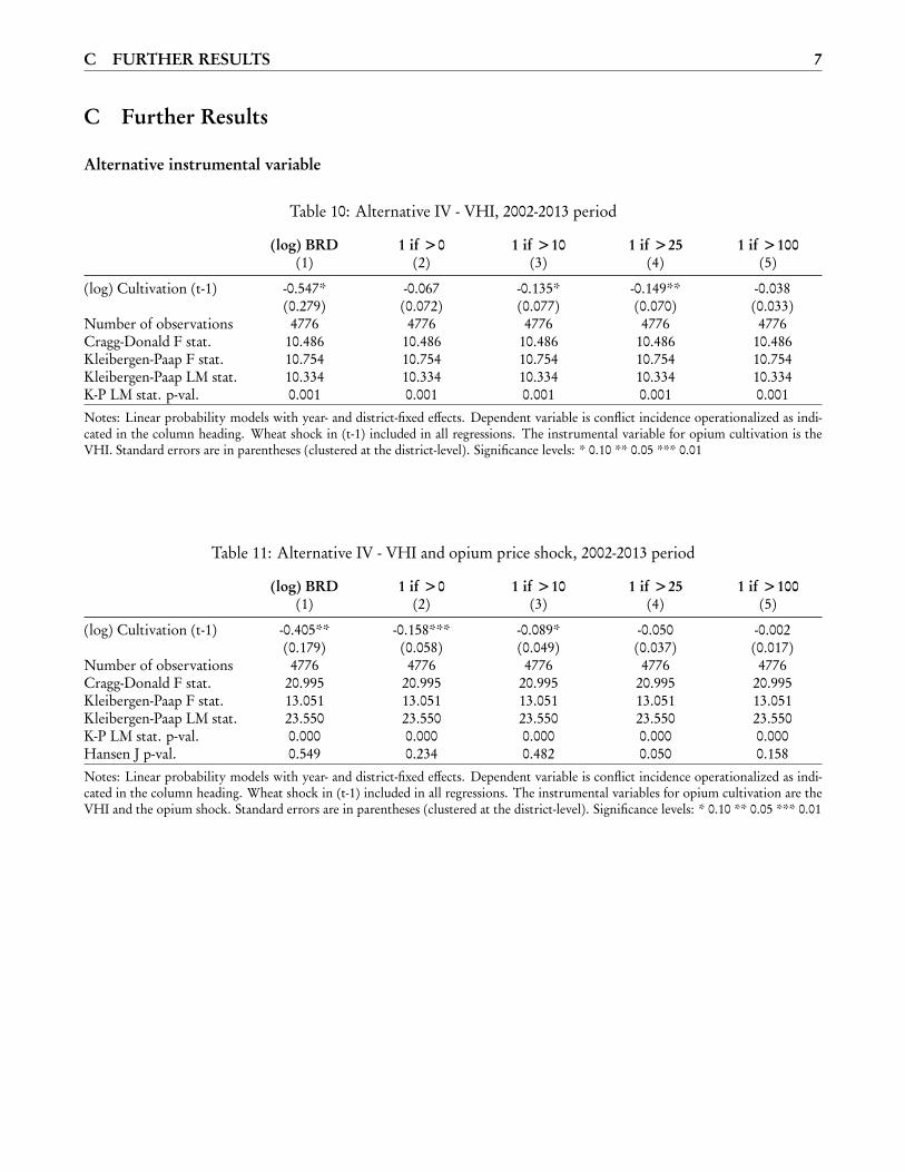
C FURTHER RESULTS 7
C Further Results
Alternative instrumental variable
Table 10: Alternative IV - VHI, 2002-2013 period
(log) BRD 1 if >0 1 if >10 1 if >25 1 if >100(1) (2) (3) (4) (5)
(log) Cultivation (t-1) -0.547* -0.067 -0.135* -0.149** -0.038(0.279) (0.072) (0.077) (0.070) (0.033)
Number of observations 4776 4776 4776 4776 4776Cragg-Donald F stat. 10.486 10.486 10.486 10.486 10.486Kleibergen-Paap F stat. 10.754 10.754 10.754 10.754 10.754Kleibergen-Paap LM stat. 10.334 10.334 10.334 10.334 10.334K-P LM stat. p-val. 0.001 0.001 0.001 0.001 0.001Notes: Linear probability models with year- and district-fixed effects. Dependent variable is conflict incidence operationalized as indi-cated in the column heading. Wheat shock in (t-1) included in all regressions. The instrumental variable for opium cultivation is theVHI. Standard errors are in parentheses (clustered at the district-level). Significance levels: * 0.10 ** 0.05 *** 0.01
Table 11: Alternative IV - VHI and opium price shock, 2002-2013 period
(log) BRD 1 if >0 1 if >10 1 if >25 1 if >100(1) (2) (3) (4) (5)
(log) Cultivation (t-1) -0.405** -0.158*** -0.089* -0.050 -0.002(0.179) (0.058) (0.049) (0.037) (0.017)
Number of observations 4776 4776 4776 4776 4776Cragg-Donald F stat. 20.995 20.995 20.995 20.995 20.995Kleibergen-Paap F stat. 13.051 13.051 13.051 13.051 13.051Kleibergen-Paap LM stat. 23.550 23.550 23.550 23.550 23.550K-P LM stat. p-val. 0.000 0.000 0.000 0.000 0.000Hansen J p-val. 0.549 0.234 0.482 0.050 0.158Notes: Linear probability models with year- and district-fixed effects. Dependent variable is conflict incidence operationalized as indi-cated in the column heading. Wheat shock in (t-1) included in all regressions. The instrumental variables for opium cultivation are theVHI and the opium shock. Standard errors are in parentheses (clustered at the district-level). Significance levels: * 0.10 ** 0.05 *** 0.01
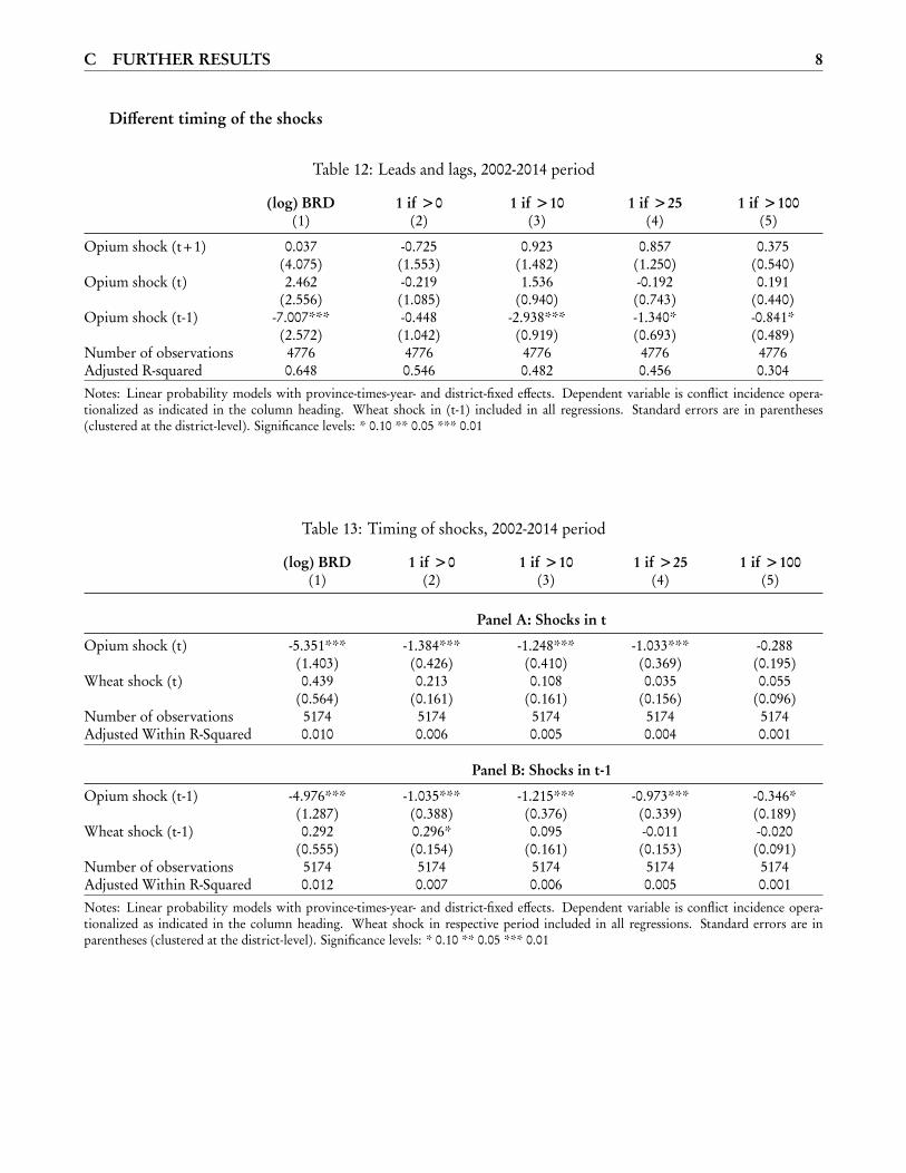
C FURTHER RESULTS 8
Different timing of the shocks
Table 12: Leads and lags, 2002-2014 period
(log) BRD 1 if >0 1 if >10 1 if >25 1 if >100(1) (2) (3) (4) (5)
Opium shock (t+1) 0.037 -0.725 0.923 0.857 0.375(4.075) (1.553) (1.482) (1.250) (0.540)
Opium shock (t) 2.462 -0.219 1.536 -0.192 0.191(2.556) (1.085) (0.940) (0.743) (0.440)
Opium shock (t-1) -7.007*** -0.448 -2.938*** -1.340* -0.841*(2.572) (1.042) (0.919) (0.693) (0.489)
Number of observations 4776 4776 4776 4776 4776Adjusted R-squared 0.648 0.546 0.482 0.456 0.304Notes: Linear probability models with province-times-year- and district-fixed effects. Dependent variable is conflict incidence opera-tionalized as indicated in the column heading. Wheat shock in (t-1) included in all regressions. Standard errors are in parentheses(clustered at the district-level). Significance levels: * 0.10 ** 0.05 *** 0.01
Table 13: Timing of shocks, 2002-2014 period
(log) BRD 1 if >0 1 if >10 1 if >25 1 if >100(1) (2) (3) (4) (5)
Panel A: Shocks in t
Opium shock (t) -5.351*** -1.384*** -1.248*** -1.033*** -0.288(1.403) (0.426) (0.410) (0.369) (0.195)
Wheat shock (t) 0.439 0.213 0.108 0.035 0.055(0.564) (0.161) (0.161) (0.156) (0.096)
Number of observations 5174 5174 5174 5174 5174Adjusted Within R-Squared 0.010 0.006 0.005 0.004 0.001
Panel B: Shocks in t-1
Opium shock (t-1) -4.976*** -1.035*** -1.215*** -0.973*** -0.346*(1.287) (0.388) (0.376) (0.339) (0.189)
Wheat shock (t-1) 0.292 0.296* 0.095 -0.011 -0.020(0.555) (0.154) (0.161) (0.153) (0.091)
Number of observations 5174 5174 5174 5174 5174Adjusted Within R-Squared 0.012 0.007 0.006 0.005 0.001Notes: Linear probability models with province-times-year- and district-fixed effects. Dependent variable is conflict incidence opera-tionalized as indicated in the column heading. Wheat shock in respective period included in all regressions. Standard errors are inparentheses (clustered at the district-level). Significance levels: * 0.10 ** 0.05 *** 0.01
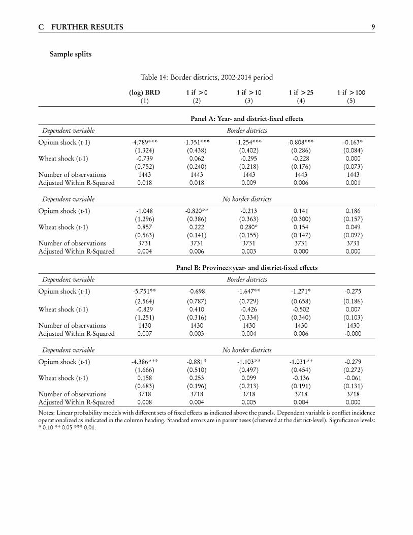
C FURTHER RESULTS 9
Sample splits
Table 14: Border districts, 2002-2014 period
(log) BRD 1 if >0 1 if >10 1 if >25 1 if >100(1) (2) (3) (4) (5)
Panel A: Year- and district-fixed effects
Dependent variable Border districts
Opium shock (t-1) -4.789*** -1.351*** -1.254*** -0.808*** -0.163*(1.324) (0.438) (0.402) (0.286) (0.084)
Wheat shock (t-1) -0.739 0.062 -0.295 -0.228 0.000(0.752) (0.240) (0.218) (0.176) (0.073)
Number of observations 1443 1443 1443 1443 1443Adjusted Within R-Squared 0.018 0.018 0.009 0.006 0.001
Dependent variable No border districts
Opium shock (t-1) -1.048 -0.820** -0.213 0.141 0.186(1.296) (0.386) (0.363) (0.300) (0.157)
Wheat shock (t-1) 0.857 0.222 0.280* 0.154 0.049(0.563) (0.141) (0.155) (0.147) (0.097)
Number of observations 3731 3731 3731 3731 3731Adjusted Within R-Squared 0.004 0.006 0.003 0.000 0.000
Panel B: Province×year- and district-fixed effects
Dependent variable Border districts
Opium shock (t-1) -5.751** -0.698 -1.647** -1.271* -0.275(2.564) (0.787) (0.729) (0.658) (0.186)
Wheat shock (t-1) -0.829 0.410 -0.426 -0.502 0.007(1.251) (0.316) (0.334) (0.340) (0.103)
Number of observations 1430 1430 1430 1430 1430Adjusted Within R-Squared 0.007 0.003 0.004 0.006 -0.000
Dependent variable No border districts
Opium shock (t-1) -4.386*** -0.881* -1.103** -1.031** -0.279(1.666) (0.510) (0.497) (0.454) (0.272)
Wheat shock (t-1) 0.158 0.253 0.099 -0.136 -0.061(0.683) (0.196) (0.213) (0.191) (0.131)
Number of observations 3718 3718 3718 3718 3718Adjusted Within R-Squared 0.008 0.004 0.005 0.004 0.000Notes: Linear probability models with different sets of fixed effects as indicated above the panels. Dependent variable is conflict incidenceoperationalized as indicated in the column heading. Standard errors are in parentheses (clustered at the district-level). Significance levels:* 0.10 ** 0.05 *** 0.01.
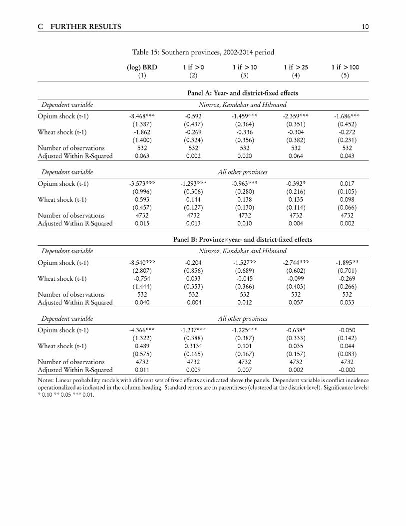
C FURTHER RESULTS 10
Table 15: Southern provinces, 2002-2014 period
(log) BRD 1 if >0 1 if >10 1 if >25 1 if >100(1) (2) (3) (4) (5)
Panel A: Year- and district-fixed effects
Dependent variable Nimroz, Kandahar and Hilmand
Opium shock (t-1) -8.468*** -0.592 -1.459*** -2.359*** -1.686***(1.387) (0.437) (0.364) (0.351) (0.452)
Wheat shock (t-1) -1.862 -0.269 -0.336 -0.304 -0.272(1.400) (0.324) (0.356) (0.382) (0.231)
Number of observations 532 532 532 532 532Adjusted Within R-Squared 0.063 0.002 0.020 0.064 0.043
Dependent variable All other provinces
Opium shock (t-1) -3.573*** -1.293*** -0.963*** -0.392* 0.017(0.996) (0.306) (0.280) (0.216) (0.105)
Wheat shock (t-1) 0.593 0.144 0.138 0.135 0.098(0.457) (0.127) (0.130) (0.114) (0.066)
Number of observations 4732 4732 4732 4732 4732Adjusted Within R-Squared 0.015 0.013 0.010 0.004 0.002
Panel B: Province×year- and district-fixed effects
Dependent variable Nimroz, Kandahar and Hilmand
Opium shock (t-1) -8.540*** -0.204 -1.527** -2.744*** -1.895**(2.807) (0.856) (0.689) (0.602) (0.701)
Wheat shock (t-1) -0.754 0.033 -0.045 -0.099 -0.269(1.444) (0.353) (0.366) (0.403) (0.266)
Number of observations 532 532 532 532 532Adjusted Within R-Squared 0.040 -0.004 0.012 0.057 0.033
Dependent variable All other provinces
Opium shock (t-1) -4.366*** -1.237*** -1.225*** -0.638* -0.050(1.322) (0.388) (0.387) (0.333) (0.142)
Wheat shock (t-1) 0.489 0.313* 0.101 0.035 0.044(0.575) (0.165) (0.167) (0.157) (0.083)
Number of observations 4732 4732 4732 4732 4732Adjusted Within R-Squared 0.011 0.009 0.007 0.002 -0.000Notes: Linear probability models with different sets of fixed effects as indicated above the panels. Dependent variable is conflict incidenceoperationalized as indicated in the column heading. Standard errors are in parentheses (clustered at the district-level). Significance levels:* 0.10 ** 0.05 *** 0.01.
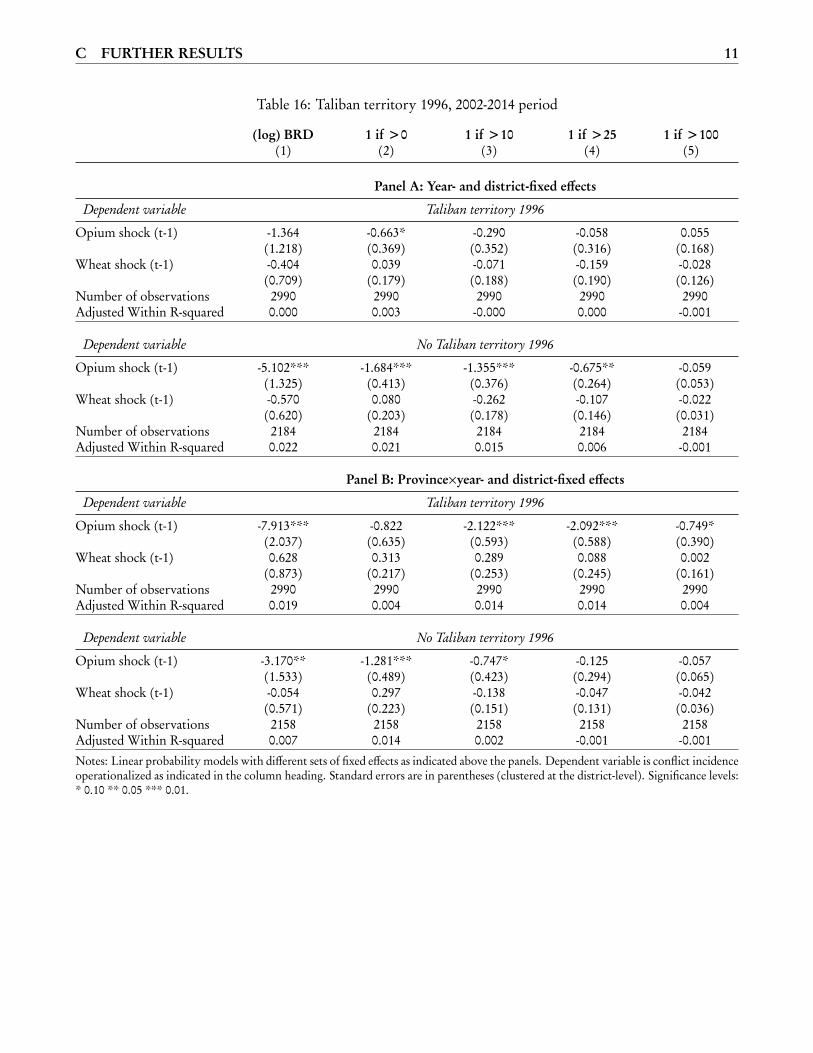
C FURTHER RESULTS 11
Table 16: Taliban territory 1996, 2002-2014 period
(log) BRD 1 if >0 1 if >10 1 if >25 1 if >100(1) (2) (3) (4) (5)
Panel A: Year- and district-fixed effects
Dependent variable Taliban territory 1996
Opium shock (t-1) -1.364 -0.663* -0.290 -0.058 0.055(1.218) (0.369) (0.352) (0.316) (0.168)
Wheat shock (t-1) -0.404 0.039 -0.071 -0.159 -0.028(0.709) (0.179) (0.188) (0.190) (0.126)
Number of observations 2990 2990 2990 2990 2990Adjusted Within R-squared 0.000 0.003 -0.000 0.000 -0.001
Dependent variable No Taliban territory 1996
Opium shock (t-1) -5.102*** -1.684*** -1.355*** -0.675** -0.059(1.325) (0.413) (0.376) (0.264) (0.053)
Wheat shock (t-1) -0.570 0.080 -0.262 -0.107 -0.022(0.620) (0.203) (0.178) (0.146) (0.031)
Number of observations 2184 2184 2184 2184 2184Adjusted Within R-squared 0.022 0.021 0.015 0.006 -0.001
Panel B: Province×year- and district-fixed effects
Dependent variable Taliban territory 1996
Opium shock (t-1) -7.913*** -0.822 -2.122*** -2.092*** -0.749*(2.037) (0.635) (0.593) (0.588) (0.390)
Wheat shock (t-1) 0.628 0.313 0.289 0.088 0.002(0.873) (0.217) (0.253) (0.245) (0.161)
Number of observations 2990 2990 2990 2990 2990Adjusted Within R-squared 0.019 0.004 0.014 0.014 0.004
Dependent variable No Taliban territory 1996
Opium shock (t-1) -3.170** -1.281*** -0.747* -0.125 -0.057(1.533) (0.489) (0.423) (0.294) (0.065)
Wheat shock (t-1) -0.054 0.297 -0.138 -0.047 -0.042(0.571) (0.223) (0.151) (0.131) (0.036)
Number of observations 2158 2158 2158 2158 2158Adjusted Within R-squared 0.007 0.014 0.002 -0.001 -0.001Notes: Linear probability models with different sets of fixed effects as indicated above the panels. Dependent variable is conflict incidenceoperationalized as indicated in the column heading. Standard errors are in parentheses (clustered at the district-level). Significance levels:* 0.10 ** 0.05 *** 0.01.
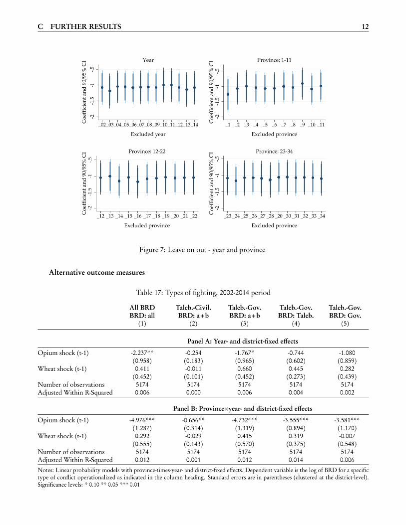
C FURTHER RESULTS 12
-2-1
.5-1
-.5C
oeffi
cien
t and
90/
95%
CI
_02_03_04_05_06_07_08_09_10_11_12_13_14
Excluded year
Year
-2-1
.5-1
-.5C
oeffi
cien
t and
90/
95%
CI
_1 _2 _3 _4 _5 _6 _7 _8 _9 _10 _11
Excluded province
Province: 1-11
-2-1
.5-1
-.5C
oeffi
cien
t and
90/
95%
CI
_12 _13 _14 _15 _16 _17 _18 _19 _20 _21 _22
Excluded province
Province: 12-22
-2-1
.5-1
-.5C
oeffi
cien
t and
90/
95%
CI
_23 _24 _25 _26 _27 _28 _20 _30 _31 _32 _33 _34
Excluded province
Province: 23-34
Figure 7: Leave on out - year and province
Alternative outcome measures
Table 17: Types of fighting, 2002-2014 period
All BRD Taleb.-Civil. Taleb.-Gov. Taleb.-Gov. Taleb.-Gov.BRD: all BRD: a+b BRD: a+b BRD: Taleb. BRD: Gov.
(1) (2) (3) (4) (5)
Panel A: Year- and district-fixed effects
Opium shock (t-1) -2.237** -0.254 -1.767* -0.744 -1.080(0.958) (0.183) (0.965) (0.602) (0.859)
Wheat shock (t-1) 0.411 -0.011 0.660 0.445 0.282(0.452) (0.101) (0.452) (0.273) (0.439)
Number of observations 5174 5174 5174 5174 5174Adjusted Within R-Squared 0.006 0.000 0.006 0.004 0.002
Panel B: Province×year- and district-fixed effects
Opium shock (t-1) -4.976*** -0.656** -4.732*** -3.555*** -3.581***(1.287) (0.314) (1.319) (0.894) (1.170)
Wheat shock (t-1) 0.292 -0.029 0.415 0.319 -0.007(0.555) (0.143) (0.570) (0.375) (0.548)
Number of observations 5174 5174 5174 5174 5174Adjusted Within R-Squared 0.012 0.001 0.012 0.014 0.006Notes: Linear probability models with province-times-year- and district-fixed effects. Dependent variable is the log of BRD for a specifictype of conflict operationalized as indicated in the column heading. Standard errors are in parentheses (clustered at the district-level).Significance levels: * 0.10 ** 0.05 *** 0.01
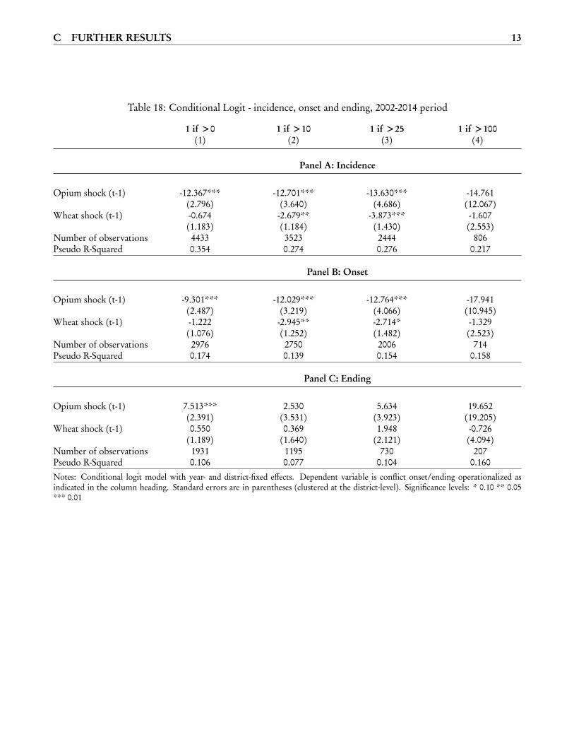
C FURTHER RESULTS 13
Table 18: Conditional Logit - incidence, onset and ending, 2002-2014 period
1 if >0 1 if >10 1 if >25 1 if >100(1) (2) (3) (4)
Panel A: Incidence
Opium shock (t-1) -12.367*** -12.701*** -13.630*** -14.761(2.796) (3.640) (4.686) (12.067)
Wheat shock (t-1) -0.674 -2.679** -3.873*** -1.607(1.183) (1.184) (1.430) (2.553)
Number of observations 4433 3523 2444 806Pseudo R-Squared 0.354 0.274 0.276 0.217
Panel B: Onset
Opium shock (t-1) -9.301*** -12.029*** -12.764*** -17.941(2.487) (3.219) (4.066) (10.945)
Wheat shock (t-1) -1.222 -2.945** -2.714* -1.329(1.076) (1.252) (1.482) (2.523)
Number of observations 2976 2750 2006 714Pseudo R-Squared 0.174 0.139 0.154 0.158
Panel C: Ending
Opium shock (t-1) 7.513*** 2.530 5.634 19.652(2.391) (3.531) (3.923) (19.205)
Wheat shock (t-1) 0.550 0.369 1.948 -0.726(1.189) (1.640) (2.121) (4.094)
Number of observations 1931 1195 730 207Pseudo R-Squared 0.106 0.077 0.104 0.160Notes: Conditional logit model with year- and district-fixed effects. Dependent variable is conflict onset/ending operationalized asindicated in the column heading. Standard errors are in parentheses (clustered at the district-level). Significance levels: * 0.10 ** 0.05*** 0.01
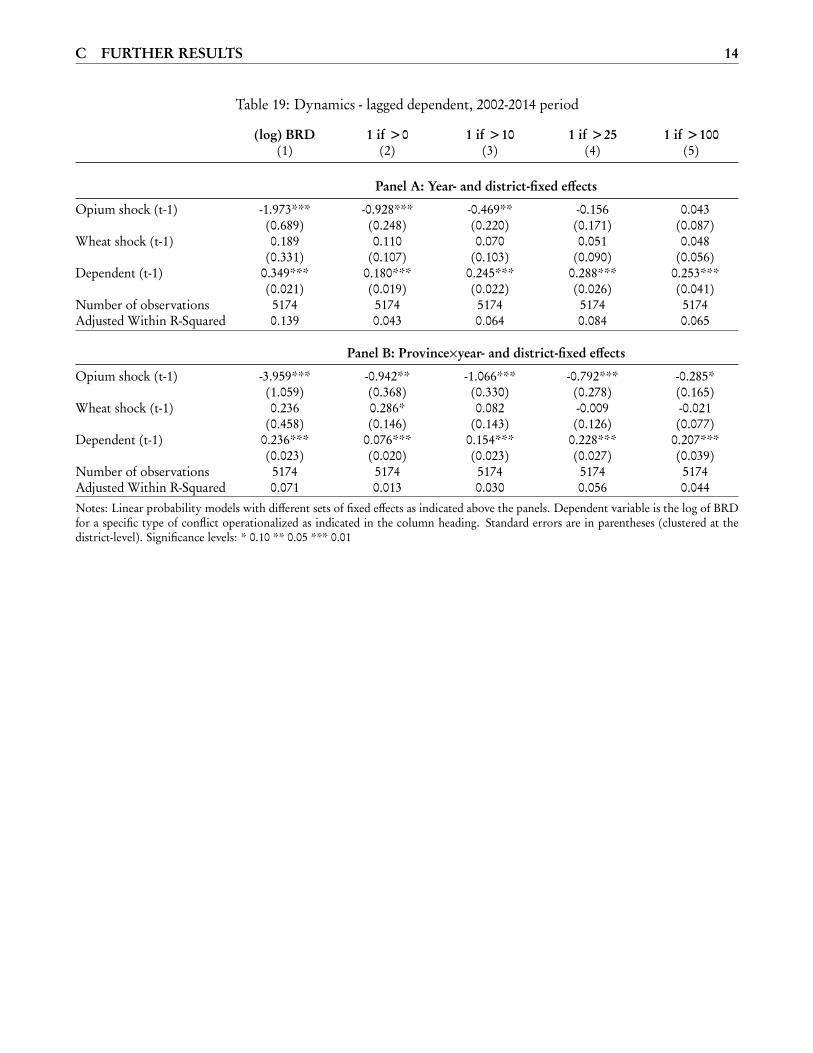
C FURTHER RESULTS 14
Table 19: Dynamics - lagged dependent, 2002-2014 period
(log) BRD 1 if >0 1 if >10 1 if >25 1 if >100(1) (2) (3) (4) (5)
Panel A: Year- and district-fixed effects
Opium shock (t-1) -1.973*** -0.928*** -0.469** -0.156 0.043(0.689) (0.248) (0.220) (0.171) (0.087)
Wheat shock (t-1) 0.189 0.110 0.070 0.051 0.048(0.331) (0.107) (0.103) (0.090) (0.056)
Dependent (t-1) 0.349*** 0.180*** 0.245*** 0.288*** 0.253***(0.021) (0.019) (0.022) (0.026) (0.041)
Number of observations 5174 5174 5174 5174 5174Adjusted Within R-Squared 0.139 0.043 0.064 0.084 0.065
Panel B: Province×year- and district-fixed effects
Opium shock (t-1) -3.959*** -0.942** -1.066*** -0.792*** -0.285*(1.059) (0.368) (0.330) (0.278) (0.165)
Wheat shock (t-1) 0.236 0.286* 0.082 -0.009 -0.021(0.458) (0.146) (0.143) (0.126) (0.077)
Dependent (t-1) 0.236*** 0.076*** 0.154*** 0.228*** 0.207***(0.023) (0.020) (0.023) (0.027) (0.039)
Number of observations 5174 5174 5174 5174 5174Adjusted Within R-Squared 0.071 0.013 0.030 0.056 0.044Notes: Linear probability models with different sets of fixed effects as indicated above the panels. Dependent variable is the log of BRDfor a specific type of conflict operationalized as indicated in the column heading. Standard errors are in parentheses (clustered at thedistrict-level). Significance levels: * 0.10 ** 0.05 *** 0.01
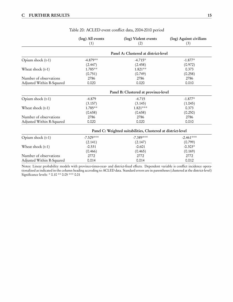
C FURTHER RESULTS 15
Table 20: ACLED event conflict data, 2004-2010 period
(log) All events (log) Violent events (log) Against civilians(1) (2) (3)
Panel A: Clustered at district-level
Opium shock (t-1) -4.879** -4.715* -1.877*(2.447) (2.458) (0.972)
Wheat shock (t-1) 1.785** 1.821** 0.373(0.751) (0.749) (0.258)
Number of observations 2786 2786 2786Adjusted Within R-Squared 0.020 0.020 0.010
Panel B: Clustered at province-level
Opium shock (t-1) -4.879 -4.715 -1.877*(3.157) (3.145) (1.045)
Wheat shock (t-1) 1.785** 1.821*** 0.373(0.658) (0.658) (0.250)
Number of observations 2786 2786 2786Adjusted Within R-Squared 0.020 0.020 0.010
Panel C: Weighted suitabilities, Clustered at district-level
Opium shock (t-1) -7.529*** -7.389*** -2.461***(2.141) (2.147) (0.799)
Wheat shock (t-1) -0.531 -0.601 -0.303*(0.466) (0.465) (0.169)
Number of observations 2772 2772 2772Adjusted Within R-Squared 0.014 0.014 0.012Notes: Linear probability models with province-times-year- and district-fixed effects. Dependent variable is conflict incidence opera-tionalized as indicated in the column heading accroding to ACLED data. Standard errors are in parentheses (clustered at the district-level)Significance levels: * 0.10 ** 0.05 *** 0.01
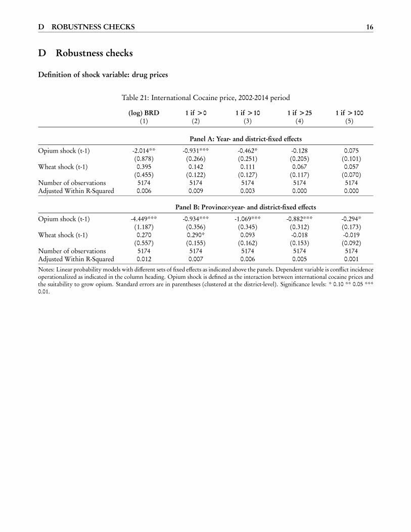
D ROBUSTNESS CHECKS 16
D Robustness checks
Definition of shock variable: drug prices
Table 21: International Cocaine price, 2002-2014 period
(log) BRD 1 if >0 1 if >10 1 if >25 1 if >100(1) (2) (3) (4) (5)
Panel A: Year- and district-fixed effects
Opium shock (t-1) -2.014** -0.931*** -0.462* -0.128 0.075(0.878) (0.266) (0.251) (0.205) (0.101)
Wheat shock (t-1) 0.395 0.142 0.111 0.067 0.057(0.455) (0.122) (0.127) (0.117) (0.070)
Number of observations 5174 5174 5174 5174 5174Adjusted Within R-Squared 0.006 0.009 0.003 0.000 0.000
Panel B: Province×year- and district-fixed effects
Opium shock (t-1) -4.449*** -0.934*** -1.069*** -0.882*** -0.294*(1.187) (0.356) (0.345) (0.312) (0.173)
Wheat shock (t-1) 0.270 0.290* 0.093 -0.018 -0.019(0.557) (0.155) (0.162) (0.153) (0.092)
Number of observations 5174 5174 5174 5174 5174Adjusted Within R-Squared 0.012 0.007 0.006 0.005 0.001Notes: Linear probability models with different sets of fixed effects as indicated above the panels. Dependent variable is conflict incidenceoperationalized as indicated in the column heading. Opium shock is defined as the interaction between international cocaine prices andthe suitability to grow opium. Standard errors are in parentheses (clustered at the district-level). Significance levels: * 0.10 ** 0.05 ***0.01.
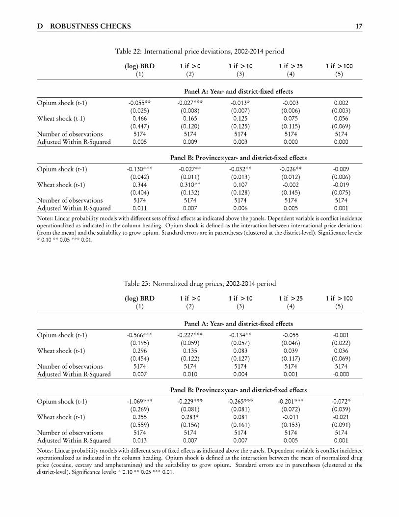
D ROBUSTNESS CHECKS 17
Table 22: International price deviations, 2002-2014 period
(log) BRD 1 if >0 1 if >10 1 if >25 1 if >100(1) (2) (3) (4) (5)
Panel A: Year- and district-fixed effects
Opium shock (t-1) -0.055** -0.027*** -0.013* -0.003 0.002(0.025) (0.008) (0.007) (0.006) (0.003)
Wheat shock (t-1) 0.466 0.165 0.125 0.075 0.056(0.447) (0.120) (0.125) (0.115) (0.069)
Number of observations 5174 5174 5174 5174 5174Adjusted Within R-Squared 0.005 0.009 0.003 0.000 0.000
Panel B: Province×year- and district-fixed effects
Opium shock (t-1) -0.130*** -0.027** -0.032** -0.026** -0.009(0.042) (0.011) (0.013) (0.012) (0.006)
Wheat shock (t-1) 0.344 0.310** 0.107 -0.002 -0.019(0.404) (0.132) (0.128) (0.145) (0.075)
Number of observations 5174 5174 5174 5174 5174Adjusted Within R-Squared 0.011 0.007 0.006 0.005 0.001Notes: Linear probability models with different sets of fixed effects as indicated above the panels. Dependent variable is conflict incidenceoperationalized as indicated in the column heading. Opium shock is defined as the interaction between international price deviations(from the mean) and the suitability to grow opium. Standard errors are in parentheses (clustered at the district-level). Significance levels:* 0.10 ** 0.05 *** 0.01.
Table 23: Normalized drug prices, 2002-2014 period
(log) BRD 1 if >0 1 if >10 1 if >25 1 if >100(1) (2) (3) (4) (5)
Panel A: Year- and district-fixed effects
Opium shock (t-1) -0.566*** -0.227*** -0.134** -0.055 -0.001(0.195) (0.059) (0.057) (0.046) (0.022)
Wheat shock (t-1) 0.296 0.135 0.083 0.039 0.036(0.454) (0.122) (0.127) (0.117) (0.069)
Number of observations 5174 5174 5174 5174 5174Adjusted Within R-Squared 0.007 0.010 0.004 0.001 -0.000
Panel B: Province×year- and district-fixed effects
Opium shock (t-1) -1.069*** -0.229*** -0.265*** -0.201*** -0.072*(0.269) (0.081) (0.081) (0.072) (0.039)
Wheat shock (t-1) 0.255 0.283* 0.081 -0.011 -0.021(0.559) (0.156) (0.161) (0.153) (0.091)
Number of observations 5174 5174 5174 5174 5174Adjusted Within R-Squared 0.013 0.007 0.007 0.005 0.001Notes: Linear probability models with different sets of fixed effects as indicated above the panels. Dependent variable is conflict incidenceoperationalized as indicated in the column heading. Opium shock is defined as the interaction between the mean of normalized drugprice (cocaine, ecstasy and amphetamines) and the suitability to grow opium. Standard errors are in parentheses (clustered at thedistrict-level). Significance levels: * 0.10 ** 0.05 *** 0.01.
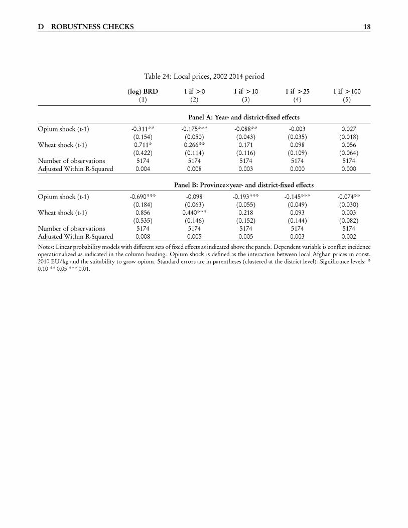
D ROBUSTNESS CHECKS 18
Table 24: Local prices, 2002-2014 period
(log) BRD 1 if >0 1 if >10 1 if >25 1 if >100(1) (2) (3) (4) (5)
Panel A: Year- and district-fixed effects
Opium shock (t-1) -0.311** -0.175*** -0.088** -0.003 0.027(0.154) (0.050) (0.043) (0.035) (0.018)
Wheat shock (t-1) 0.711* 0.266** 0.171 0.098 0.056(0.422) (0.114) (0.116) (0.109) (0.064)
Number of observations 5174 5174 5174 5174 5174Adjusted Within R-Squared 0.004 0.008 0.003 0.000 0.000
Panel B: Province×year- and district-fixed effects
Opium shock (t-1) -0.690*** -0.098 -0.193*** -0.145*** -0.074**(0.184) (0.063) (0.055) (0.049) (0.030)
Wheat shock (t-1) 0.856 0.440*** 0.218 0.093 0.003(0.535) (0.146) (0.152) (0.144) (0.082)
Number of observations 5174 5174 5174 5174 5174Adjusted Within R-Squared 0.008 0.005 0.005 0.003 0.002Notes: Linear probability models with different sets of fixed effects as indicated above the panels. Dependent variable is conflict incidenceoperationalized as indicated in the column heading. Opium shock is defined as the interaction between local Afghan prices in const.2010 EU/kg and the suitability to grow opium. Standard errors are in parentheses (clustered at the district-level). Significance levels: *0.10 ** 0.05 *** 0.01.
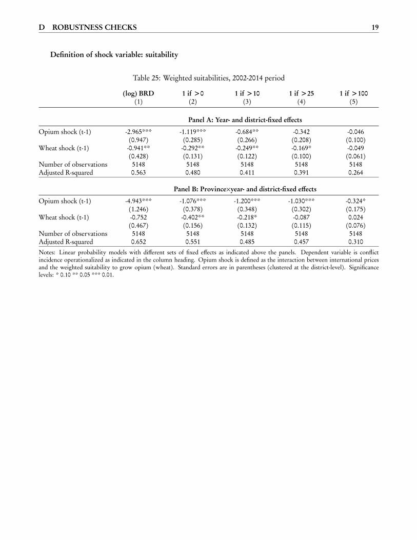
D ROBUSTNESS CHECKS 19
Definition of shock variable: suitability
Table 25: Weighted suitabilities, 2002-2014 period
(log) BRD 1 if >0 1 if >10 1 if >25 1 if >100(1) (2) (3) (4) (5)
Panel A: Year- and district-fixed effects
Opium shock (t-1) -2.965*** -1.119*** -0.684** -0.342 -0.046(0.947) (0.285) (0.266) (0.208) (0.100)
Wheat shock (t-1) -0.941** -0.292** -0.249** -0.169* -0.049(0.428) (0.131) (0.122) (0.100) (0.061)
Number of observations 5148 5148 5148 5148 5148Adjusted R-squared 0.563 0.480 0.411 0.391 0.264
Panel B: Province×year- and district-fixed effects
Opium shock (t-1) -4.943*** -1.076*** -1.200*** -1.030*** -0.324*(1.246) (0.378) (0.348) (0.302) (0.175)
Wheat shock (t-1) -0.752 -0.402** -0.218* -0.087 0.024(0.467) (0.156) (0.132) (0.115) (0.076)
Number of observations 5148 5148 5148 5148 5148Adjusted R-squared 0.652 0.551 0.485 0.457 0.310Notes: Linear probability models with different sets of fixed effects as indicated above the panels. Dependent variable is conflictincidence operationalized as indicated in the column heading. Opium shock is defined as the interaction between international pricesand the weighted suitability to grow opium (wheat). Standard errors are in parentheses (clustered at the district-level). Significancelevels: * 0.10 ** 0.05 *** 0.01.
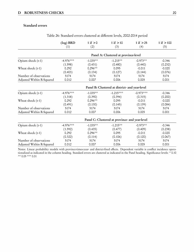
D ROBUSTNESS CHECKS 20
Standard errors
Table 26: Standard errors clustered at different levels, 2002-2014 period
(log) BRD 1 if >0 1 if >10 1 if >25 1 if >100(1) (2) (3) (4) (5)
Panel A: Clustered at province-level
Opium shock (t-1) -4.976*** -1.035** -1.215** -0.973** -0.346(1.598) (0.431) (0.480) (0.440) (0.232)
Wheat shock (t-1) 0.292 0.296** 0.095 -0.011 -0.020(0.403) (0.134) (0.127) (0.144) (0.076)
Number of observations 5174 5174 5174 5174 5174Adjusted Within R-Squared 0.012 0.007 0.006 0.005 0.001
Panel B: Clustered at district- and year-level
Opium shock (t-1) -4.976*** -1.035** -1.215*** -0.973*** -0.346(1.318) (0.390) (0.394) (0.315) (0.200)
Wheat shock (t-1) 0.292 0.296** 0.095 -0.011 -0.020(0.491) (0.130) (0.145) (0.139) (0.084)
Number of observations 5174 5174 5174 5174 5174Adjusted Within R-Squared 0.012 0.007 0.006 0.005 0.001
Panel C: Clustered at province- and year-level
Opium shock (t-1) -4.976*** -1.035** -1.215** -0.973** -0.346(1.592) (0.435) (0.477) (0.409) (0.238)
Wheat shock (t-1) 0.292 0.296** 0.095 -0.011 -0.020(0.322) (0.114) (0.106) (0.120) (0.067)
Number of observations 5174 5174 5174 5174 5174Adjusted Within R-Squared 0.012 0.007 0.006 0.005 0.001Notes: Linear probability models with province-times-year- and district-fixed effects. Dependent variable is conflict incidence opera-tionalized as indicated in the column heading. Standard errors are clustered as indicated in the Panel heading. Significance levels: * 0.10** 0.05 *** 0.01
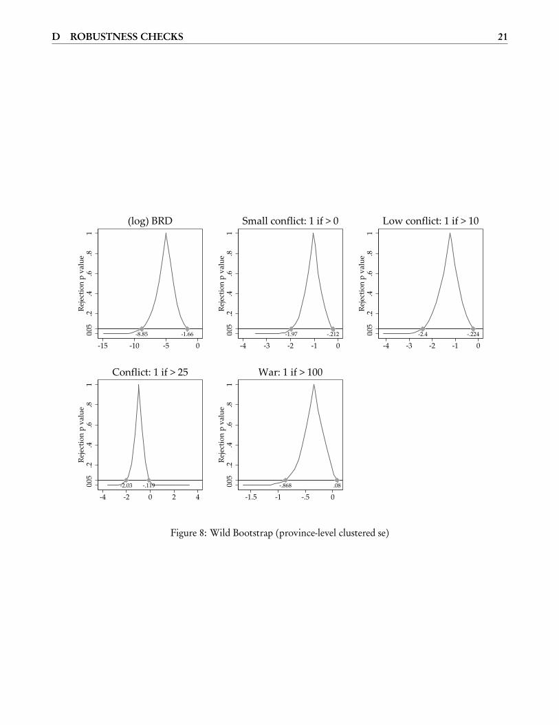
D ROBUSTNESS CHECKS 21
-8.85 -1.660.2
.4.6
.81
.05
Reje
ctio
n p
valu
e
-15 -10 -5 0
(log) BRD
-1.97 -.2120.2
.4.6
.81
.05
Reje
ctio
n p
valu
e
-4 -3 -2 -1 0
Small conflict: 1 if > 0
-2.4 -.2240.2
.4.6
.81
.05
Reje
ctio
n p
valu
e
-4 -3 -2 -1 0
Low conflict: 1 if > 10
-2.03 -.1190.2
.4.6
.81
.05
Reje
ctio
n p
valu
e
-4 -2 0 2 4
Conflict: 1 if > 25
-.868 .080.2
.4.6
.81
.05
Reje
ctio
n p
valu
e
-1.5 -1 -.5 0
War: 1 if > 100
Figure 8: Wild Bootstrap (province-level clustered se)
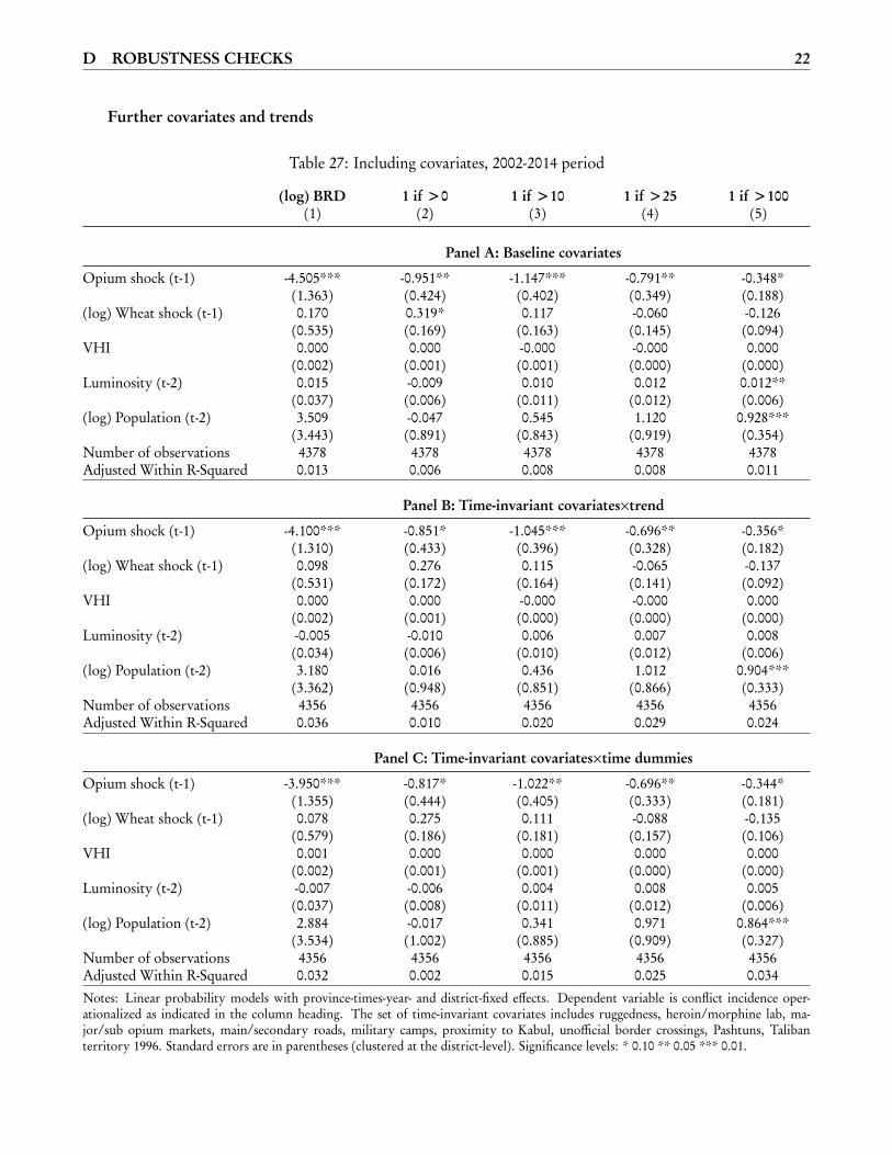
D ROBUSTNESS CHECKS 22
Further covariates and trends
Table 27: Including covariates, 2002-2014 period
(log) BRD 1 if >0 1 if >10 1 if >25 1 if >100(1) (2) (3) (4) (5)
Panel A: Baseline covariates
Opium shock (t-1) -4.505*** -0.951** -1.147*** -0.791** -0.348*(1.363) (0.424) (0.402) (0.349) (0.188)
(log) Wheat shock (t-1) 0.170 0.319* 0.117 -0.060 -0.126(0.535) (0.169) (0.163) (0.145) (0.094)
VHI 0.000 0.000 -0.000 -0.000 0.000(0.002) (0.001) (0.001) (0.000) (0.000)
Luminosity (t-2) 0.015 -0.009 0.010 0.012 0.012**(0.037) (0.006) (0.011) (0.012) (0.006)
(log) Population (t-2) 3.509 -0.047 0.545 1.120 0.928***(3.443) (0.891) (0.843) (0.919) (0.354)
Number of observations 4378 4378 4378 4378 4378Adjusted Within R-Squared 0.013 0.006 0.008 0.008 0.011
Panel B: Time-invariant covariates×trend
Opium shock (t-1) -4.100*** -0.851* -1.045*** -0.696** -0.356*(1.310) (0.433) (0.396) (0.328) (0.182)
(log) Wheat shock (t-1) 0.098 0.276 0.115 -0.065 -0.137(0.531) (0.172) (0.164) (0.141) (0.092)
VHI 0.000 0.000 -0.000 -0.000 0.000(0.002) (0.001) (0.000) (0.000) (0.000)
Luminosity (t-2) -0.005 -0.010 0.006 0.007 0.008(0.034) (0.006) (0.010) (0.012) (0.006)
(log) Population (t-2) 3.180 0.016 0.436 1.012 0.904***(3.362) (0.948) (0.851) (0.866) (0.333)
Number of observations 4356 4356 4356 4356 4356Adjusted Within R-Squared 0.036 0.010 0.020 0.029 0.024
Panel C: Time-invariant covariates×time dummies
Opium shock (t-1) -3.950*** -0.817* -1.022** -0.696** -0.344*(1.355) (0.444) (0.405) (0.333) (0.181)
(log) Wheat shock (t-1) 0.078 0.275 0.111 -0.088 -0.135(0.579) (0.186) (0.181) (0.157) (0.106)
VHI 0.001 0.000 0.000 0.000 0.000(0.002) (0.001) (0.001) (0.000) (0.000)
Luminosity (t-2) -0.007 -0.006 0.004 0.008 0.005(0.037) (0.008) (0.011) (0.012) (0.006)
(log) Population (t-2) 2.884 -0.017 0.341 0.971 0.864***(3.534) (1.002) (0.885) (0.909) (0.327)
Number of observations 4356 4356 4356 4356 4356Adjusted Within R-Squared 0.032 0.002 0.015 0.025 0.034Notes: Linear probability models with province-times-year- and district-fixed effects. Dependent variable is conflict incidence oper-ationalized as indicated in the column heading. The set of time-invariant covariates includes ruggedness, heroin/morphine lab, ma-jor/sub opium markets, main/secondary roads, military camps, proximity to Kabul, unofficial border crossings, Pashtuns, Talibanterritory 1996. Standard errors are in parentheses (clustered at the district-level). Significance levels: * 0.10 ** 0.05 *** 0.01.
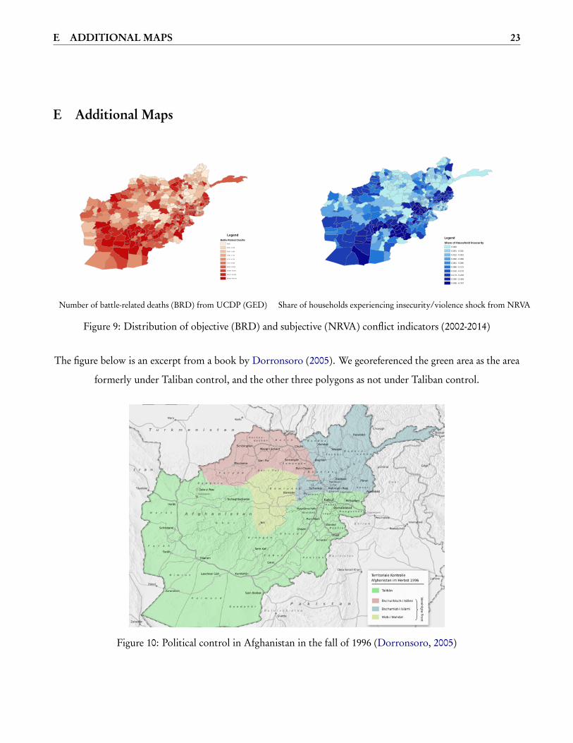
E ADDITIONAL MAPS 23
E Additional Maps
Battle-Related Deaths
LegendBattle-Related Deaths
0.000
0.000 - 0.428
0.428 - 1.285
1.286 - 2.714
2.714 - 4.714
4.714 - 6.929
6.929 - 10.929
10.929 - 18.571
18.571 - 36.429
36.429 - 446.071
LegendShare of Household Insecurity
0.0000.001 - 0.0110.012 - 0.0310.032 - 0.0600.061 - 0.0950.096 - 0.1310.132 - 0.1720.173 - 0.2590.260 - 0.4340.435 - 0.767
Number of battle-related deaths (BRD) from UCDP (GED) Share of households experiencing insecurity/violence shock from NRVA
Figure 9: Distribution of objective (BRD) and subjective (NRVA) conflict indicators (2002-2014)
The figure below is an excerpt from a book by Dorronsoro (2005). We georeferenced the green area as the area
formerly under Taliban control, and the other three polygons as not under Taliban control.
Figure 10: Political control in Afghanistan in the fall of 1996 (Dorronsoro, 2005)
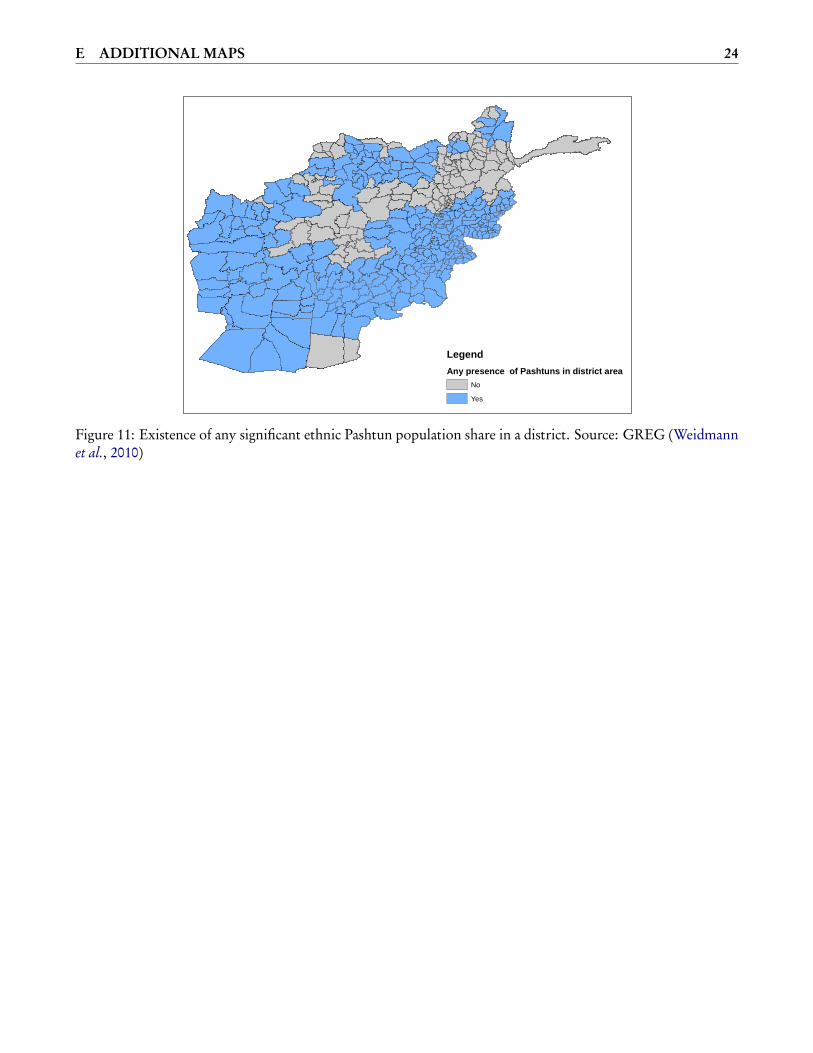
E ADDITIONAL MAPS 24
LegendAny presence of Pashtuns in district area
NoYes
Figure 11: Existence of any significant ethnic Pashtun population share in a district. Source: GREG (Weidmannet al., 2010)
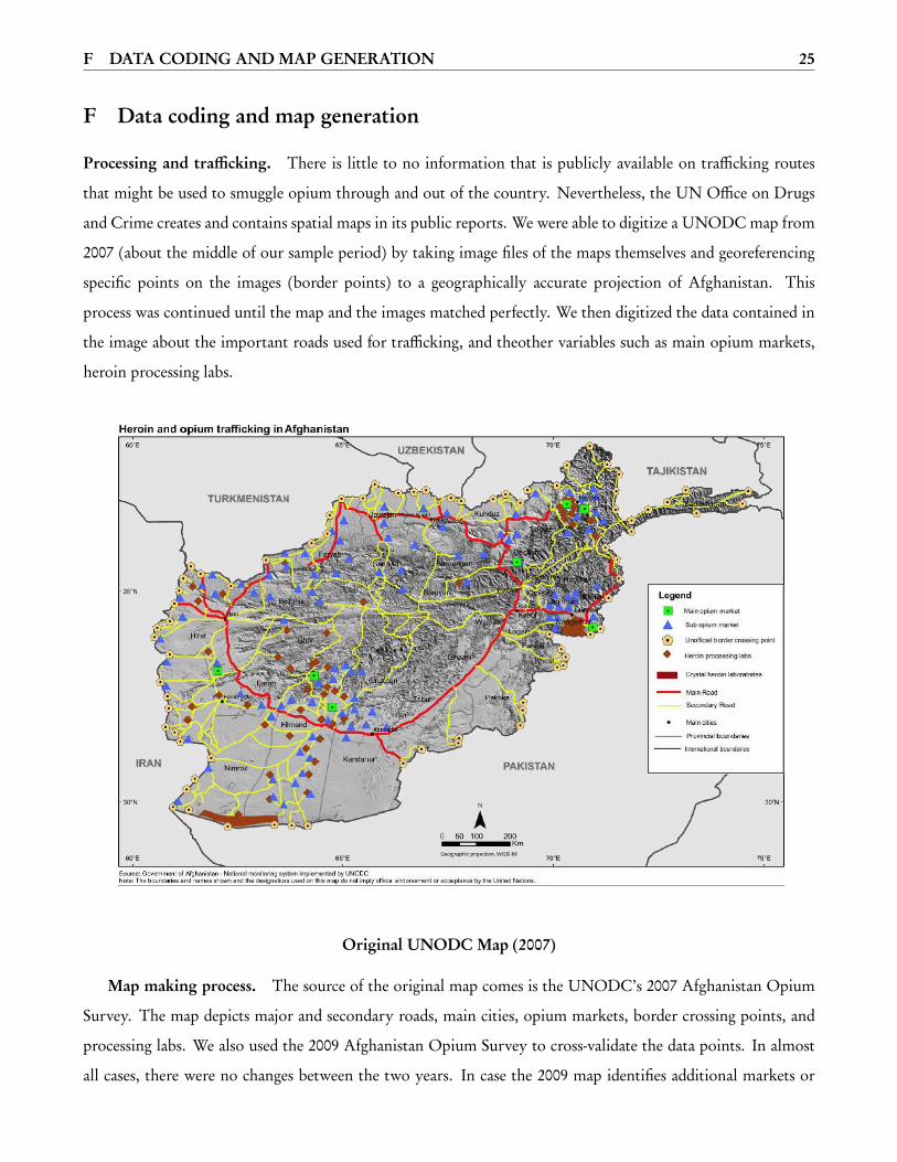
F DATA CODING AND MAP GENERATION 25
F Data coding and map generation
Processing and trafficking. There is little to no information that is publicly available on trafficking routes
that might be used to smuggle opium through and out of the country. Nevertheless, the UN Office on Drugs
and Crime creates and contains spatial maps in its public reports. We were able to digitize a UNODC map from
2007 (about the middle of our sample period) by taking image files of the maps themselves and georeferencing
specific points on the images (border points) to a geographically accurate projection of Afghanistan. This
process was continued until the map and the images matched perfectly. We then digitized the data contained in
the image about the important roads used for trafficking, and theother variables such as main opium markets,
heroin processing labs.
Original UNODC Map (2007)
Map making process. The source of the original map comes is the UNODC’s 2007 Afghanistan Opium
Survey. The map depicts major and secondary roads, main cities, opium markets, border crossing points, and
processing labs. We also used the 2009 Afghanistan Opium Survey to cross-validate the data points. In almost
all cases, there were no changes between the two years. In case the 2009 map identifies additional markets or
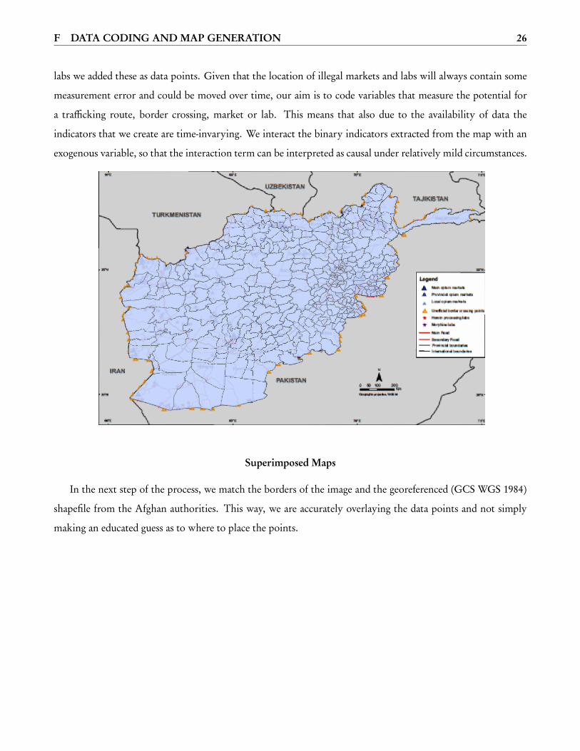
F DATA CODING AND MAP GENERATION 26
labs we added these as data points. Given that the location of illegal markets and labs will always contain some
measurement error and could be moved over time, our aim is to code variables that measure the potential for
a trafficking route, border crossing, market or lab. This means that also due to the availability of data the
indicators that we create are time-invarying. We interact the binary indicators extracted from the map with an
exogenous variable, so that the interaction term can be interpreted as causal under relatively mild circumstances.
Superimposed Maps
In the next step of the process, we match the borders of the image and the georeferenced (GCS WGS 1984)
shapefile from the Afghan authorities. This way, we are accurately overlaying the data points and not simply
making an educated guess as to where to place the points.
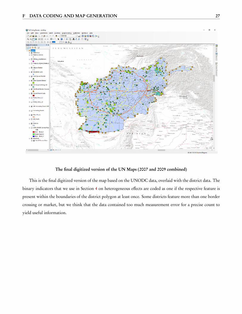
F DATA CODING AND MAP GENERATION 27
The final digitized version of the UN Maps (2007 and 2009 combined)
This is the final digitized version of the map based on the UNODC data, overlaid with the district data. The
binary indicators that we use in Section 4 on heterogeneous effects are coded as one if the respective feature is
present within the boundaries of the district polygon at least once. Some districts feature more than one border
crossing or market, but we think that the data contained too much measurement error for a precise count to
yield useful information.
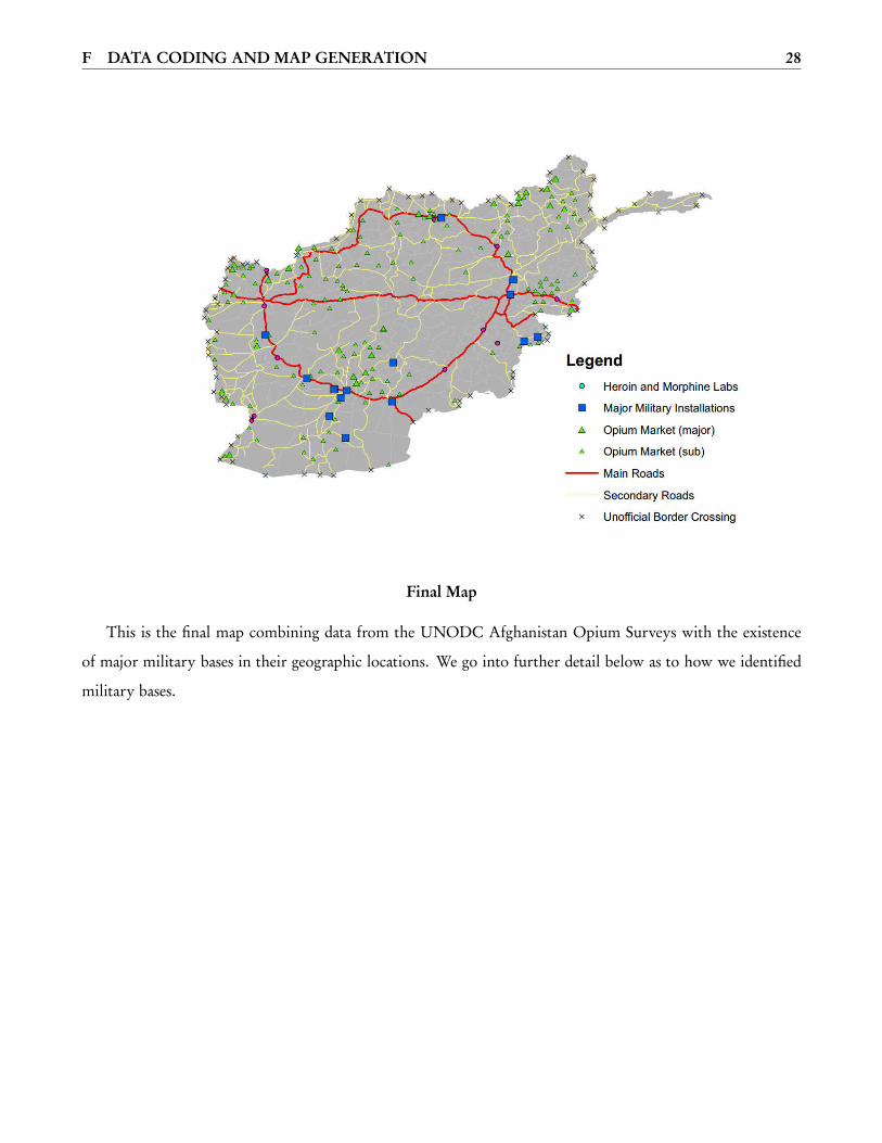
F DATA CODING AND MAP GENERATION 28
Final Map
This is the final map combining data from the UNODC Afghanistan Opium Surveys with the existence
of major military bases in their geographic locations. We go into further detail below as to how we identified
military bases.
F DATA CODING AND MAP GENERATION 29
Major military bases. This section describes how we determine the locations of major known military bases
in Afghanistan. There are nearly 400 foreign military bases in Afghanistan, but none of these bases release
information as to their geographic location for security reasons. In order to find this information, we compiled
what data we could to determine which bases were most important to include, where exactly (latitude and
longitude coordinates) these bases are (or were; many are now closed) and a number of other important variables
(see tables below). We ended up relying on information from Wikipedia’s GeoHack program for the more well-
known bases and on news articles, and Wikimapia and Google Maps satellite data for the less well-documented
ones. News articles were useful in this case because they are often allowed to publish the district in which
these bases are located; from there, we were able to look for these bases by referencing photos of hte bases (if
available) with available satelite data. Below, we show where and how we got the locations of 54 important bases
and where the latitude and longitude coordinates lead to on a map.
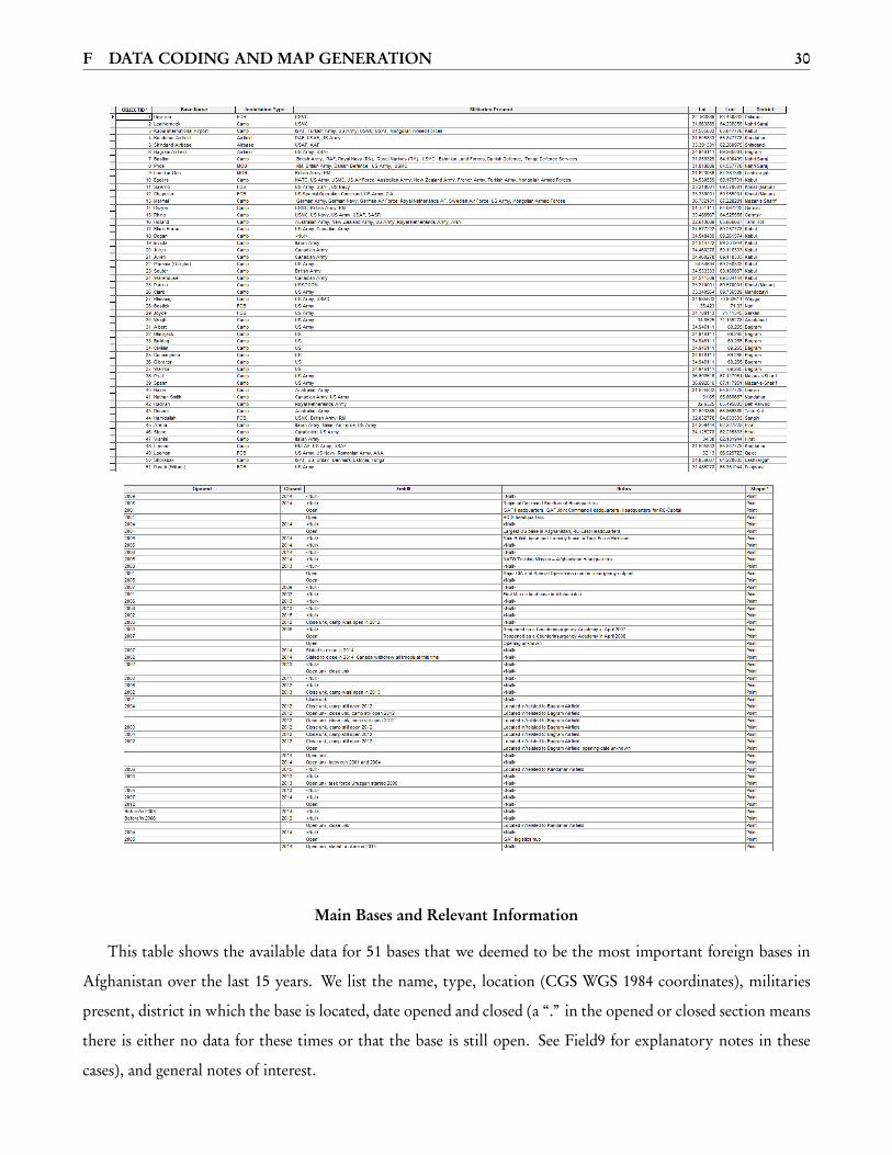
F DATA CODING AND MAP GENERATION 30
Main Bases and Relevant Information
This table shows the available data for 51 bases that we deemed to be the most important foreign bases in
Afghanistan over the last 15 years. We list the name, type, location (CGS WGS 1984 coordinates), militaries
present, district in which the base is located, date opened and closed (a “.” in the opened or closed section means
there is either no data for these times or that the base is still open. See Field9 for explanatory notes in these
cases), and general notes of interest.
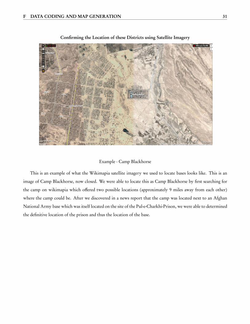
F DATA CODING AND MAP GENERATION 31
Confirming the Location of these Districts using Satellite Imagery
Example - Camp Blackhorse
This is an example of what the Wikimapia satellite imagery we used to locate bases looks like. This is an
image of Camp Blackhorse, now closed. We were able to locate this as Camp Blackhorse by first searching for
the camp on wikimapia which offered two possible locations (approximately 9 miles away from each other)
where the camp could be. After we discovered in a news report that the camp was located next to an Afghan
National Army base which was itself located on the site of the Pul-e-Charkhi-Prison, we were able to determined
the definitive location of the prison and thus the location of the base.
F DATA CODING AND MAP GENERATION 32
Definitions and explanation of how each base was found. Below, we have laid out the definitions for
what each type of base exists in Afghanistan and explained how we determined the specific locations for each
base we included. The base definitions are important to know because the type of base is a good indicator of
its size. Though this was of course not the only criteria we used to determine whether or not a specific base
should be represented on the map, it was important for weeding out those that are ot included (for example, we
included no firebases on account of their temporary and generally small size. Below this, we go into detail about
specific bases whose locations we were not able to get from the GeoHack database, in which bases are supposed
to have had multiple confirmations. These bases were found using satelite data and through confirming guesses
that some people have made on Wikimapia using any available news reports, photos and satelite imagery.
• Definition FOB - A forward operating base (FOB) is any secured forward military position, commonly
a military base, that is used to support tactical operations. A FOB may or may not contain an airfield,
hospital, or other facilities. The base may be used for an extended period of time. FOBs are traditionally
supported by Main Operating Bases that are required to provide backup support to them. A FOB also
improves reaction time to local areas as opposed to having all troops on the main operating base.
• Definition MOB - is a term used by the United States military defined as a "permanently manned, well
protected base, used to support permanently deployed forces, and with robust sea and/or air access." Not
so significant,
• Definition COP - a combat outpost is a detachment of troops stationed at a distance from the main force
or formation, usually at a station in a remote or sparsely populated location, positioned to stand guard
against unauthorized intrusions and surprise attacks; and the station occupied by such troops, usually a
small military base or settlement in an outlying frontier, limit, political boundary or in another country.
(Small, about 32 guys. People walking not driving, very small reach, 20km
• Definition Firebase - a temporary military encampment to provide artillery fire support to infantry oper-
ating in areas beyond the normal range of fire support from their own base camps.
• Definition Camp - a semi-permanent facility for the lodging of an army. Camps are erected when a
military force travels away from a major installation or fort during training or operations, and often have
the form of large campsites. Weird definition.
• Definition Base - a facility directly owned and operated by or for the military or one of its branches that
shelters military equipment and personnel, and facilitates training and operations. In general, a military
base provides accommodations for one or more units, but it may also be used as a command center, a
F DATA CODING AND MAP GENERATION 33
training ground, or a proving ground. In most cases, a military base relies on some outside help in order
to operate. However, certain complex bases are able to endure by themselves for long periods because
they are able to provide food, water and other life support necessities for their inhabitants while under
siege. *All definitions from Wikipedia
All locations taken from Wikimedia’s GeoHack program unless referenced as otherwise below:
1. COP/FOB Zangabad has been coded as FOB Pasab. This was the most likely location for a forward op-
erating base close the Zhari/Panjwayi district border. Exact location determined as such using Wikimapia
satelite imagery. It is coded as being in the district of Panjwayi.
2. Camp/FOB Hadrian location determined using Wikimapia satelite imagery.
3. Camp Russell location determined using Wikimapia satelite imagery in relation to Camp Holland.
4. Camp Arena, Camp Vianini, and Camp Stone are each in roughly the same area. Using Wikimapia
imagery, we assume that Camp Arena, the only camp with an Italian Air Force presence, is located at the
airfield in Hirat. Camp Vianini and Camp Stone were assigned their locations using Wikimapia imagery
as well. We believe Camp Vianini to be at the location we chose based on the fact that an Italian artillery
regiment was attacked at that location and we believe the Italian Army was the only major force at Camp
Vianini. Camp Stone, which has multiple country forces at its location, is expected to be south of the
airport and Camp Arena, according to Wikimapia data.
5. Camp Blackhorse determined using Wikimapia and various sources citing the camp to be adjacent to the
Pul-e-Charkhi ANA compound.
6. Camp Clark determined using Wikimapia satelite imagery.
7. Camp Warehouse determined using Wikimapia stelite imagery.
8. Camp Phoenix lcoation determined using google maps and Wikimapia satelite data.
9. Camp Invicta located using Wikimapia satelite data.
10. FOB Hamidullah located using Wikimapia satelite data. In Wikimapia, the location is described as FOB
Nolay, the previous name of the base.
11. Camp Blessing located using Wikimapia satelite data.
12. FOB Joyce located using satelite data and with news articles stating that FOB Joyce is within/very close
to the village of Serkanay.
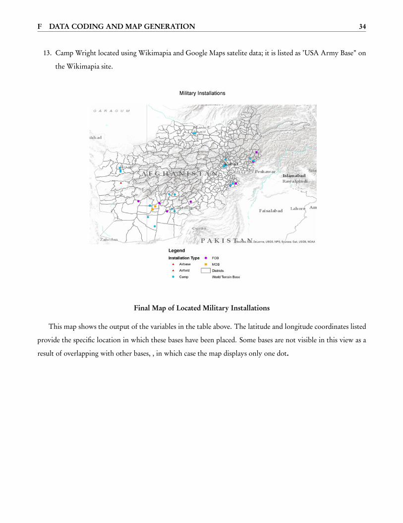
F DATA CODING AND MAP GENERATION 34
13. Camp Wright located using Wikimapia and Google Maps satelite data; it is listed as ’USA Army Base" on
the Wikimapia site.
Final Map of Located Military Installations
This map shows the output of the variables in the table above. The latitude and longitude coordinates listed
provide the specific location in which these bases have been placed. Some bases are not visible in this view as a
result of overlapping with other bases, , in which case the map displays only one dot.