1

An opium curse? The long-run economic

consequences of narcotics cultivation in British India

Jonathan Lehne1

June 10 2018

Abstract

The long run consequences of colonial rule depended on the institutions introduced by the

colonisers and the economic activities they promoted. This paper analyses the effects of opium

production under British rule on current economic development in India. I employ a border

discontinuity design which interacts fine-grained local variation in environmental suitability

for poppy cultivation with administrative boundaries that demarcated opium-growing areas. I

find that greater suitability for opium is associated with lower literacy and a lower rate of public

good provision within opium-growing districts but has no effect in bordering areas where

opium cultivation was prohibited. Placebo tests using suitability for other crops show no such

discontinuity. Colonial administrative data allows me to test potential mechanisms for the

persistent negative effect of opium production. Greater opium cultivation is associated with

less per capita public spending on health and education by the British administration, a lower

number of schools, and a greater concentration of police officers. These results suggest that

colonial officials in opium growing districts concentrated on administering and policing the

extraction of monopsony rents, while investing less in the wider local economy.

Keywords: colonialism, long-run development, resource curse

1 Paris School of Economics; Boulevard Jourdan 48, 75014 Paris, France; jonathan.lehne@gmail.com

2

1. Introduction

The state-sponsored export of opium from British India to China was arguably the largest and

most enduring drug operation in history. At its peak in the mid-19th century it accounted for

roughly 15% of total colonial revenue in India and 31% of India’s exports (Richards 2002). To

supply this trade the East India Company (EIC) – and later the British Government – developed

a highly regulated cultivation system in which over one million farmers a year were under

contract to grow opium poppies.2 This paper evaluates the impact of this production on the

long-term development of opium-growing areas and finds that it led to lower literacy and a

lower rate of public good provision as measured by modern census data.

An influential literature in economics relates contemporary outcomes to the policies and

institutions introduced by former colonial powers. Engerman and Sokoloff (2000), and

Acemoglu, Johnson and Robinson (2001, 2002) argue that colonial rulers implemented

different institutions depending on the factor endowments they encountered. Recent work has

sought to build on these theories and add specificity by exploiting within-country variation in

colonial policies and rich historical datasets not available at the cross-country level (Dell 2010,

Dell and Olken 2017, Lowes and Montero 2017). While the British opium agencies were

unique institutions – implementing the large-scale production of a narcotic for a government

with strictly enforced monopsony rights – their long-term impacts have broader relevance for

the study of colonial legacies. I use local administrative data from the late 19th and early 20th

century to investigate how the presence of a highly lucrative resource altered colonial

administrators’ incentives and the policies they implemented with respect to the rest of the

economy.

My empirical strategy exploits the interaction between two factors that affected an area’s

likelihood of opium cultivation: geographic suitability and administrative boundaries. The

opium agencies were careful to select locations whose conditions were most adapted to

cultivation, in terms of the soil and climate, as well as the distance to the factories where raw

opium was processed (Richards 1981). However, cultivation was only permitted in certain

districts meaning that many suitable locations were left unexploited. Using a regression

discontinuity design (RDD), I compare the effect of opium suitability in villages either side of

2 In the year 1907 for example, the combined total number of cultivators in the Bihar and Benares Agencies was

over 1.3 million (Opium Department 1909).

3

the boundaries that demarcated poppy-growing regions. Under the assumption that, absent

opium cultivation, the effects of suitability would be continuous across borders, this approach

identifies the causal impact of opium production on present-day outcomes.

This empirical design relies on the ability to predict an area’s suitability for poppy cultivation.

For a significant part of the opium growing region there exist disaggregated data on the share

of agricultural land devoted to opium cultivation at the tehsil (sub-district) level from 1895 to

1905. I combine these data with GIS information on temperature, precipitation, altitude,

ruggedness, soil types, soil characteristics (e.g. soil ph), the location of rivers and lakes, and

the distance to the factories where raw opium was processed. Given the large number of

potential explanatory variables, I use the least absolute shrinkage and selection operator

(LASSO)3 to pick the variables that are the best predictors of opium cultivation and generate

an opium suitability index. As this measure is likely to be correlated with production of other

crops, I calculate similar suitability indices for other crops as well as an aggregate agricultural

suitability index. These measures are used as controls and in placebo tests, to ensure that results

are driven by suitability for poppy cultivation.

The second element of the identification strategy are administrative rules that confined opium

production to specific areas. In British India, opium cultivation was strictly controlled by local

‘sub-agencies’ who issued licenses to cultivators in their territory. As the borders of these sub-

agencies frequently coincided with colonial district boundaries, it is not reasonable to assume

that they only affected long-term development through the likelihood of opium production.

Instead, I combine the RDD with a cross-section difference-in-differences approach:

comparing villages with different suitability for poppies within the same district on both sides

of the border. If opium cultivation had significant consequences on long-term development,

the difference between suitable and unsuitable villages should be larger within former sub-

agencies than in districts where cultivation was prohibited.

I find that a higher likelihood of historical opium cultivation is negatively associated with

measures of contemporary village-level development used in the literature (e.g. Banerjee and

Iyer 2005, Iyer 2010). In a bandwidth of 20 km from the border, the relative impact of a one

standard deviation increase in the opium suitability index in poppy-growing districts is a 3.6%

(1.4 percentage point) drop in literacy, a 2.6% (2 percentage point) drop in the likelihood of

3 Using an alternative machine learning technique (random forest classification) results in a similar selection of

predictors and an opium suitability index that is highly correlated with that generated by the LASSO.

4

having a primary school in the village and a 42.5% (1.36 percentage point) drop in the

likelihood of having a healthcare facility in the village. These results are robust to controlling

for the environmental suitability for other crops, and to narrowing the bandwidth for the RDD.

My results also indicate a negative effect on the likelihood of the village having all-weather

road access, but this is only significant at the 10 km bandwidth.

Why should historical opium cultivation have had persistent impacts on human capital and

public good provision? One potential mechanism relates to the interests of the local colonial

administration which were closely intertwined with the state opium enterprise. In poppy-

growing districts – senior British officials formally took on a second role as officers of the

opium sub-agency. The literature on the natural resource curse suggests that a dominant

commodity that provides a large share of government revenue can undermine the incentives

for public good provision (Ross 2003, Caselli and Cunningham 2009). In this context, securing

the extraction of opium rents and policing the state’s monopsony power were a governmental

priority, while the incentive to invest in the wider economy may have been weaker. I provide

evidence in support of this mechanism using colonial administrative data. At the district-level,

opium production was associated with lower per capita expenditure on education and

healthcare. Sub-district-level data shows that localities with a higher suitability for opium had

fewer schools and a greater number of policemen stationed in their tehsil. These analyses are

constrained by the small sample sizes, but the results are consistent with a focus on security at

the expense of human capital and diversified economic development.

This paper contributes to the literature on the long-term consequences of colonial rule. Recent

work in this area has focussed on individual sectors in order to isolate the impact of specific

colonial policies. Dell (2010) and Lowes and Montero (2017) document persistent negative

effects of forced labour – on outcomes including public good provision – in the context of

Spanish silver mining in Peru and Belgian rubber concessions in the present-day Democratic

Republic of Congo, respectively. By contrast, Dell and Olken (2017) show that the

establishment of Dutch sugar factories in Indonesia gave rise to agglomeration effects, meaning

that nearby areas forced to grow sugar, are now more industrialised, better educated and have

better infrastructure. The contrast between sugar and opium is instructive. While the former

was a widely consumed commodity with important downstream linkages to food processing

and manufacturing, opium in India was cut off from the rest of the economy – by virtue of its

distinctive uses but also deliberate British policy. When the Dutch sugar factories closed, the

economic opportunities that had sprung up around them remained. The decline of opium

5

production in India may be more reminiscent of the depletion of a mineral resource, with few

enduring benefits.

My paper also contributes to a strand of this literature which studies the persistent effects of

different forms of colonial rule in India. Banerjee and Iyer (2005) show that landlord-based

tenure systems perpetuated by the British in some regions, led to lower agricultural investment

and productivity after independence. Iyer (2010) exploits a colonial annexation rule to compare

the effect of direct and indirect rule on long-run development, finding that areas formerly under

indirect rule have better access to schools, health centres and roads. The study of opium is

interesting in this context, because there is variation in cultivation both within British India and

between princely states. In section 6, I analyse the effect of opium suitability on literacy and

public good provision in princely states and find no significant negative effect. As I cannot

directly replicate my empirical strategy in this sample, this difference should be interpreted

with caution. One potential explanation, however, is that the private merchants who were free

to enter the trade in princely states were more likely to invest their profits locally than the EIC

or the British Government.

The remainder of this paper is structured as follows. Section 2 provides background on the

history of opium in India and the institutions the British implemented to administer production.

Section 3 describes the data used in the analysis and the construction of the agricultural

suitability indices. Section 4 explains the empirical strategy and tests the validity of

assumptions required for identification. The results are presented in Section 5. Section 6

provides evidence on potential mechanisms for the persistent effects of opium cultivation.

Section 7 concludes.

2. Background

2.1 Opium cultivation in India

The cultivation of opium in India predates the arrival of European colonial powers. It is thought

to have been first introduced by Arab traders in the 8th century (Watt 1892). Opium was

established as a lucrative cash crop in the 17th and 18th centuries as Dutch traders, and later the

EIC, bought up increasing quantities from Indian merchants in order to meet growing demand

in China. After cementing its political control over Bengal, the EIC was able to declare a state

6

monopoly on the cultivation and sale of the crop in 1772. Procurement of raw opium was

initially the purview of British contractors whose abuse of their official powers made them

“notorious” in cultivating areas (Richards 1981). Farmers were often forcibly coerced into

growing opium rather than traditional staple crops (Wright 1959), a practice which exacerbated

famines in times of crop failure (Chaudhury 2003, Ul Haq 2000). Remuneration was not always

adequate as contractors were known to force cultivators to give up their crop for less than the

cost of production. To regulate cultivation, the EIC set up official government agencies in 1797

(Sahu 1977). This ‘agency system’ remained in place until the decline of the opium trade

following the Hague International Opium Convention in 1912.

The two opium agencies of Bihar and Benares organised cultivation in large parts of the

Gangetic plain, in the present-day states of Uttar Pradesh, Bihar and Jharkhand. They were

divided into sub-agencies (11 for Bihar and 16 for the Benares agency). Outside the borders of

these sub-agencies cultivation was prohibited throughout British India. Each sub-agency was

led by a British official who commanded a network of Indian agents (known as gumashtas).

The gumashtas selected areas suitable for cultivation and negotiated with village headmen

before issuing licenses to cultivators (Richards 1981). No farmer was allowed to grow opium

without a license or to sell their crop to anyone other than the opium agency. Cultivators

received an advance that would be deducted from their final payment upon delivery of the

harvest. Farmers unable to meet their production quota fell into debt to the agency which could

be paid off in the form of future opium harvests (Allen 1853). Once harvested, the raw opium

was shipped to one of two central factories - at Ghazipur (for the Benares agency) or Patna (for

the Bihar agency) – where it was processed and packed into chests for export.

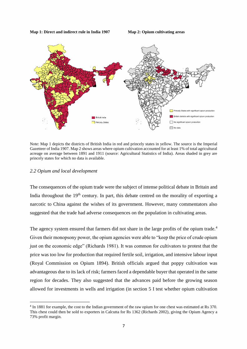
The EIC – and later the British government – were only able to enforce their monopsony inside

areas under direct British rule (see Map 1). Given the profitability of opium, various princely

states in the Malwa region of western India emerged as competitors in the early 19th century

(see Map 2). The British initially sought to curtail this trade by forbidding exports of Malwa

opium from the port of Bombay, then to control it by seeking to buy up the entire output, before

finally allowing the trade while charging a high excise fee on shipments passing through

Bombay. In section 6, I analyse whether opium cultivation is associated with negative long-

run effects in princely states, in order to distinguish between the effect of the crop per se and

the colonial institutions set up to regulate its cultivation in directly-ruled areas.

7

Map 1: Direct and indirect rule in India 1907 Map 2: Opium cultivating areas

Note: Map 1 depicts the districts of British India in red and princely states in yellow. The source is the Imperial

Gazetteer of India 1907. Map 2 shows areas where opium cultivation accounted for at least 1% of total agricultural

acreage on average between 1891 and 1911 (source: Agricultural Statistics of India). Areas shaded in grey are

princely states for which no data is available.

2.2 Opium and local development

The consequences of the opium trade were the subject of intense political debate in Britain and

India throughout the 19th century. In part, this debate centred on the morality of exporting a

narcotic to China against the wishes of its government. However, many commentators also

suggested that the trade had adverse consequences on the population in cultivating areas.

The agency system ensured that farmers did not share in the large profits of the opium trade.4

Given their monopsony power, the opium agencies were able to “keep the price of crude opium

just on the economic edge” (Richards 1981). It was common for cultivators to protest that the

price was too low for production that required fertile soil, irrigation, and intensive labour input

(Royal Commission on Opium 1894). British officials argued that poppy cultivation was

advantageous due to its lack of risk; farmers faced a dependable buyer that operated in the same

region for decades. They also suggested that the advances paid before the growing season

allowed for investments in wells and irrigation (in section 5 I test whether opium cultivation

4 In 1881 for example, the cost to the Indian government of the raw opium for one chest was estimated at Rs 370.

This chest could then be sold to exporters in Calcutta for Rs 1362 (Richards 2002), giving the Opium Agency a

73% profit margin.

8

had any lasting influence on irrigation infrastructure). In terms of long-run agricultural

development, specialising in poppies may have come at the expense of developing expertise in

other crops. By the time opium cultivation dropped sharply following the Opium Convention

in 1912, areas where growing poppies had been prohibited may have developed comparative

advantages in other crops. Moreover, other crops may have exhibited input-output linkages

leading to growth in sectors such as food processing or textiles. The agency system ensured

that poppy growing was cut off from the rest of the economy, with the only downstream activity

confined to the two government factories that processed the raw opium. In this respect, poppy

production in British India was very different from the forced sugar cultivation in Indonesia

which Dell and Olken (2017) argue had long-term benefits through agglomeration effects.

A separate set of potential developmental consequences relate to opium’s role as a narcotic. In

addition to its monopsony on raw opium, the British government had a monopoly on the sale

of opium in India. While the majority of processed opium was exported, some was sold

domestically through licensed shops. In poppy-growing areas the authorities could not control

the population’s access to unprocessed opium and contemporary sources report widespread

consumption in some regions (Royal Commission on Opium 1894). The strict price controls

also gave rise to organised smuggling which became a significant preoccupation for colonial

authorities. The government invested in a network of spies and informants and conducted anti-

smuggling drives which “often ended up harassing honest poppy cultivators” (Deshpande

2009). It is possible that poppy-growing areas suffered directly from the availability of a crop

that enabled drug use and crime.

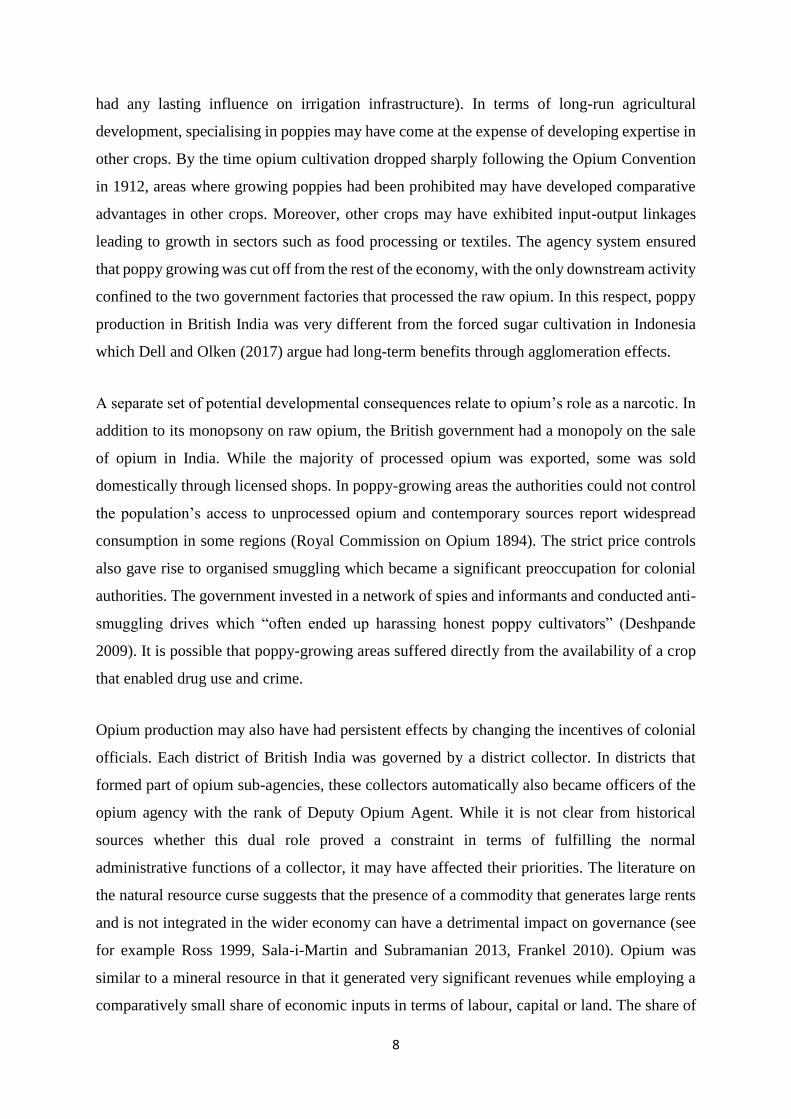
Opium production may also have had persistent effects by changing the incentives of colonial

officials. Each district of British India was governed by a district collector. In districts that

formed part of opium sub-agencies, these collectors automatically also became officers of the

opium agency with the rank of Deputy Opium Agent. While it is not clear from historical

sources whether this dual role proved a constraint in terms of fulfilling the normal

administrative functions of a collector, it may have affected their priorities. The literature on

the natural resource curse suggests that the presence of a commodity that generates large rents

and is not integrated in the wider economy can have a detrimental impact on governance (see

for example Ross 1999, Sala-i-Martin and Subramanian 2013, Frankel 2010). Opium was

similar to a mineral resource in that it generated very significant revenues while employing a

comparatively small share of economic inputs in terms of labour, capital or land. The share of

9

agricultural land in British India devoted to opium was 0.29% at its peak, but the contribution

to total colonial revenue could be as high as 15%. In opium-growing districts the average share

of agricultural land was only around 3% while the share of local economic output would be

many times higher. In this context, local officials were likely to have a large incentive to

guarantee the stable extraction of opium rents and to police the state’s monopsony and

monopoly powers. By contrast, they may have had less interest in investing in the wider local

economy, through infrastructure, education or healthcare provision than their counterparts in

districts with no opium production and no personal affiliation to the opium agencies. In section

6, I test this mechanism by evaluating the relationship between opium production and the

strength of local police forces at the time (a measure of expenditure on security) as well as the

number of local schools (a measure of human capital investment).

3. Data

This project combines colonial administrative records on agricultural production and public

services with modern census data as well as GIS information on climactic conditions. These

data at available at different levels of aggregation. Historical sources provide data either at the

level of the colonial district and princely state, or in some cases, at the level of the tehsil (sub-

district). Contemporary census data is at the village level. The GIS data used for this project

were initially at the level of a 30 arc second grid (~1 km2).

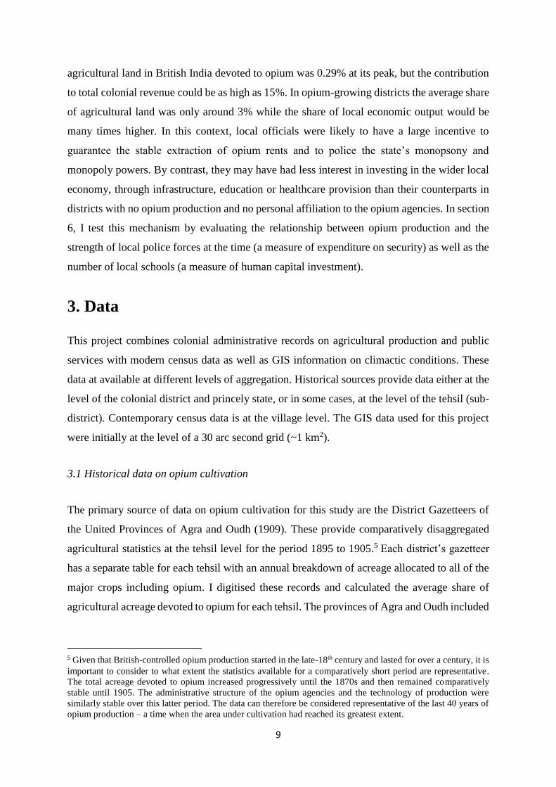
3.1 Historical data on opium cultivation

The primary source of data on opium cultivation for this study are the District Gazetteers of

the United Provinces of Agra and Oudh (1909). These provide comparatively disaggregated

agricultural statistics at the tehsil level for the period 1895 to 1905.5 Each district’s gazetteer

has a separate table for each tehsil with an annual breakdown of acreage allocated to all of the

major crops including opium. I digitised these records and calculated the average share of

agricultural acreage devoted to opium for each tehsil. The provinces of Agra and Oudh included

5 Given that British-controlled opium production started in the late-18th century and lasted for over a century, it is

important to consider to what extent the statistics available for a comparatively short period are representative.

The total acreage devoted to opium increased progressively until the 1870s and then remained comparatively

stable until 1905. The administrative structure of the opium agencies and the technology of production were

similarly stable over this latter period. The data can therefore be considered representative of the last 40 years of

opium production – a time when the area under cultivation had reached its greatest extent.

10

the entire Benares Opium Agency which accounted for roughly 70% of British-controlled

opium production during this period.

The Agricultural Statistics of India provide a less detailed but more comprehensive coverage

of opium production from 1891 to 1911. These data allow me to calculate the equivalent share

of agricultural acreage assigned to opium for all districts in British India as well as for 96

territories in former princely states.

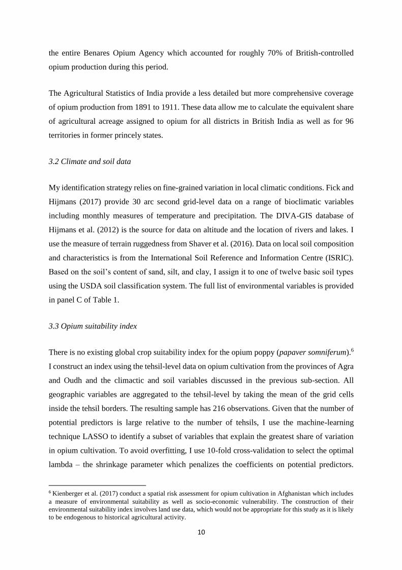
3.2 Climate and soil data

My identification strategy relies on fine-grained variation in local climatic conditions. Fick and

Hijmans (2017) provide 30 arc second grid-level data on a range of bioclimatic variables

including monthly measures of temperature and precipitation. The DIVA-GIS database of

Hijmans et al. (2012) is the source for data on altitude and the location of rivers and lakes. I

use the measure of terrain ruggedness from Shaver et al. (2016). Data on local soil composition

and characteristics is from the International Soil Reference and Information Centre (ISRIC).

Based on the soil’s content of sand, silt, and clay, I assign it to one of twelve basic soil types

using the USDA soil classification system. The full list of environmental variables is provided

in panel C of Table 1.

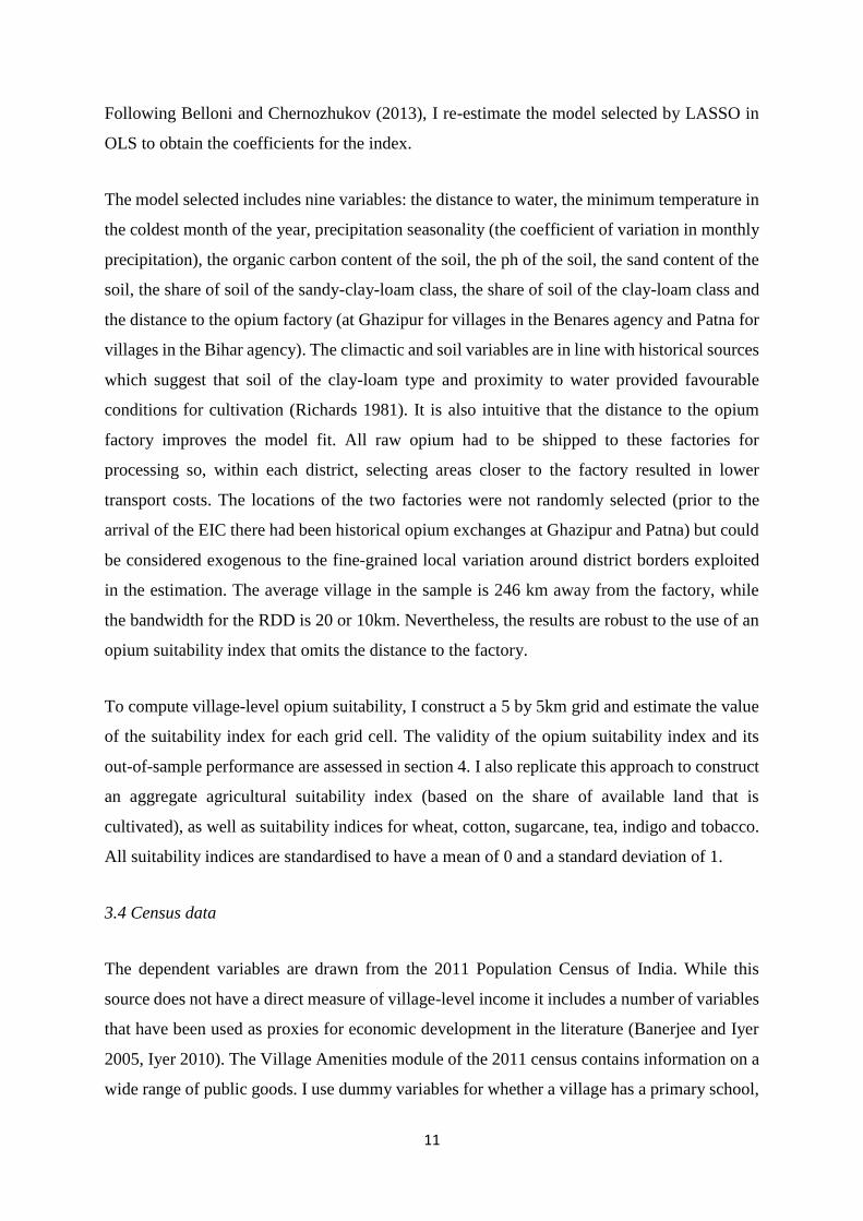
3.3 Opium suitability index

There is no existing global crop suitability index for the opium poppy (papaver somniferum).6

I construct an index using the tehsil-level data on opium cultivation from the provinces of Agra

and Oudh and the climactic and soil variables discussed in the previous sub-section. All

geographic variables are aggregated to the tehsil-level by taking the mean of the grid cells

inside the tehsil borders. The resulting sample has 216 observations. Given that the number of

potential predictors is large relative to the number of tehsils, I use the machine-learning

technique LASSO to identify a subset of variables that explain the greatest share of variation

in opium cultivation. To avoid overfitting, I use 10-fold cross-validation to select the optimal

lambda – the shrinkage parameter which penalizes the coefficients on potential predictors.

6 Kienberger et al. (2017) conduct a spatial risk assessment for opium cultivation in Afghanistan which includes

a measure of environmental suitability as well as socio-economic vulnerability. The construction of their

environmental suitability index involves land use data, which would not be appropriate for this study as it is likely

to be endogenous to historical agricultural activity.

11

Following Belloni and Chernozhukov (2013), I re-estimate the model selected by LASSO in

OLS to obtain the coefficients for the index.

The model selected includes nine variables: the distance to water, the minimum temperature in

the coldest month of the year, precipitation seasonality (the coefficient of variation in monthly

precipitation), the organic carbon content of the soil, the ph of the soil, the sand content of the

soil, the share of soil of the sandy-clay-loam class, the share of soil of the clay-loam class and

the distance to the opium factory (at Ghazipur for villages in the Benares agency and Patna for

villages in the Bihar agency). The climactic and soil variables are in line with historical sources

which suggest that soil of the clay-loam type and proximity to water provided favourable

conditions for cultivation (Richards 1981). It is also intuitive that the distance to the opium

factory improves the model fit. All raw opium had to be shipped to these factories for

processing so, within each district, selecting areas closer to the factory resulted in lower

transport costs. The locations of the two factories were not randomly selected (prior to the

arrival of the EIC there had been historical opium exchanges at Ghazipur and Patna) but could

be considered exogenous to the fine-grained local variation around district borders exploited

in the estimation. The average village in the sample is 246 km away from the factory, while

the bandwidth for the RDD is 20 or 10km. Nevertheless, the results are robust to the use of an

opium suitability index that omits the distance to the factory.

To compute village-level opium suitability, I construct a 5 by 5km grid and estimate the value

of the suitability index for each grid cell. The validity of the opium suitability index and its

out-of-sample performance are assessed in section 4. I also replicate this approach to construct

an aggregate agricultural suitability index (based on the share of available land that is

cultivated), as well as suitability indices for wheat, cotton, sugarcane, tea, indigo and tobacco.

All suitability indices are standardised to have a mean of 0 and a standard deviation of 1.

3.4 Census data

The dependent variables are drawn from the 2011 Population Census of India. While this

source does not have a direct measure of village-level income it includes a number of variables

that have been used as proxies for economic development in the literature (Banerjee and Iyer

2005, Iyer 2010). The Village Amenities module of the 2011 census contains information on a

wide range of public goods. I use dummy variables for whether a village has a primary school,

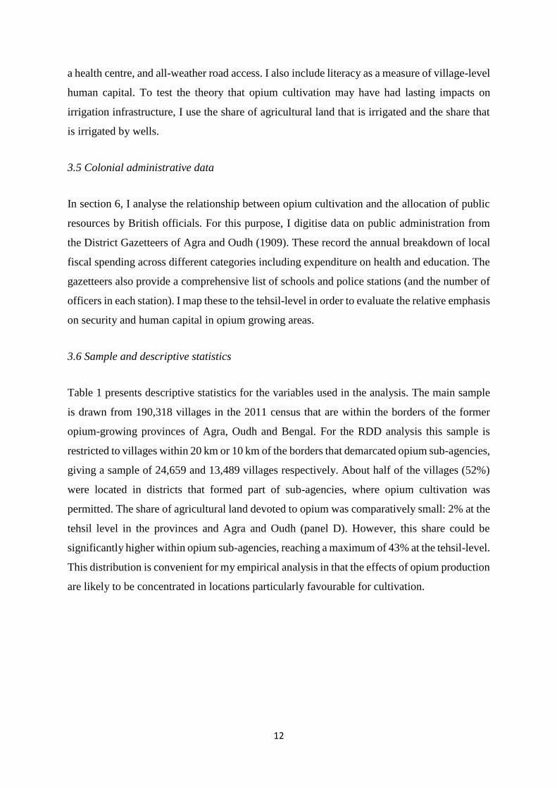
12

a health centre, and all-weather road access. I also include literacy as a measure of village-level

human capital. To test the theory that opium cultivation may have had lasting impacts on

irrigation infrastructure, I use the share of agricultural land that is irrigated and the share that

is irrigated by wells.

3.5 Colonial administrative data

In section 6, I analyse the relationship between opium cultivation and the allocation of public

resources by British officials. For this purpose, I digitise data on public administration from

the District Gazetteers of Agra and Oudh (1909). These record the annual breakdown of local

fiscal spending across different categories including expenditure on health and education. The

gazetteers also provide a comprehensive list of schools and police stations (and the number of

officers in each station). I map these to the tehsil-level in order to evaluate the relative emphasis

on security and human capital in opium growing areas.

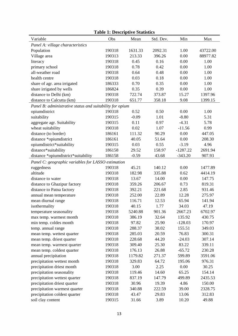
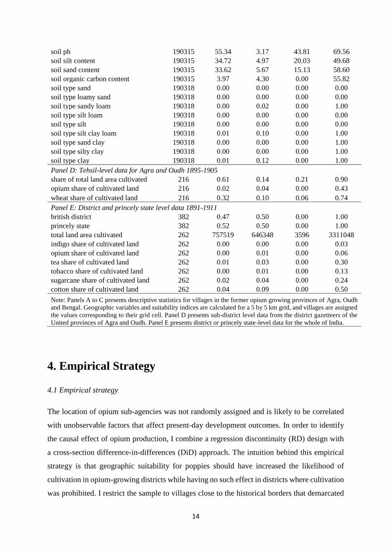
3.6 Sample and descriptive statistics

Table 1 presents descriptive statistics for the variables used in the analysis. The main sample

is drawn from 190,318 villages in the 2011 census that are within the borders of the former

opium-growing provinces of Agra, Oudh and Bengal. For the RDD analysis this sample is

restricted to villages within 20 km or 10 km of the borders that demarcated opium sub-agencies,

giving a sample of 24,659 and 13,489 villages respectively. About half of the villages (52%)

were located in districts that formed part of sub-agencies, where opium cultivation was

permitted. The share of agricultural land devoted to opium was comparatively small: 2% at the

tehsil level in the provinces and Agra and Oudh (panel D). However, this share could be

significantly higher within opium sub-agencies, reaching a maximum of 43% at the tehsil-level.

This distribution is convenient for my empirical analysis in that the effects of opium production

are likely to be concentrated in locations particularly favourable for cultivation.

13

Table 1: Descriptive Statistics

Variable Obs Mean Std. Dev. Min Max

Panel A: village characteristics

Population 190318 1631.33 2092.31 1.00 43722.00

Village area 190313 213.33 396.26 0.00 88977.82

literacy 190318 0.45 0.16 0.00 1.00

primary school 190318 0.78 0.42 0.00 1.00

all-weather road 190318 0.64 0.48 0.00 1.00

health centre 190318 0.03 0.18 0.00 1.00

share of agr. area irrigated 186333 0.70 0.35 0.00 1.00

share irrigated by wells 186824 0.35 0.39 0.00 1.00

distance to Delhi (km) 190318 722.74 373.87 15.27 1397.96

distance to Calcutta (km) 190318 651.77 358.18 9.08 1399.15

Panel B: administrative status and suitability for opium

opiumdistrict 190318 0.52 0.50 0.00 1.00

suitability 190315 -0.09 1.01 -8.80 5.31

aggregate agr. Suitability 190315 0.11 0.97 -4.31 5.78

wheat suitability 190318 0.02 1.07 -11.56 0.99

distance (to border) 186161 111.32 90.29 0.00 447.05

distance *opiumdistrict 186161 40.05 51.64 0.00 208.30

opiumdistrict*suitability 190315 0.03 0.55 -3.19 4.96

distance*suitability 186158 29.52 158.97 -1287.22 2691.94

distance *opiumdistrict*suitability 186158 -0.59 43.68 -343.20 907.93

Panel C: geographic variables for LASSO estimation

ruggedness 190318 45.21 140.12 0.00 1477.89

altitude 190318 182.98 335.88 0.62 4414.19

distance to water 190318 13.67 14.00 0.00 147.75

distance to Ghazipur factory 190318 359.26 206.67 0.73 819.31

distance to Patna factory 190318 392.21 221.68 2.85 931.46

annual mean temperature 190318 252.00 22.89 12.28 275.97

mean diurnal range 190318 116.71 12.53 65.94 141.94

isothermality 190318 40.15 1.77 34.03 47.19

temperature seasonality 190318 5240.88 901.36 2667.23 6702.97

max temp. warmest month 190318 386.19 32.64 135.92 430.75

min temp. coldes month 190318 97.82 25.90 -128.03 170.97

temp. annual range 190318 288.37 38.02 155.51 349.03

mean temp. wettest quarter 190318 285.03 20.59 76.83 300.31

mean temp. driest quarter 190318 228.68 44.20 -24.03 307.14

mean temp. warmest quarter 190318 309.40 25.30 83.22 339.11

mean temp. coldest quarter 190318 176.13 26.88 -65.72 230.28

annual precipitation 190318 1179.82 271.37 599.89 3591.06

precipitation wettest month 190318 329.83 64.72 195.06 976.31

precipitation driest month 190318 3.00 2.25 0.00 30.25

precipitation seasonality 190318 119.46 14.60 65.25 154.14

precipitation wettest quarter 190318 837.19 147.79 499.89 2435.53

precipitation driest quarter 190318 30.96 19.39 4.86 150.00

precipitation warmest quarter 190318 340.88 222.59 39.00 2328.75

precipitation coldest quarter 190318 43.47 29.83 13.06 312.83

soil clay content 190315 31.66 3.89 10.20 49.88

14

soil ph 190315 55.34 3.17 43.81 69.56

soil silt content 190315 34.72 4.97 20.03 49.68

soil sand content 190315 33.62 5.67 15.13 58.60

soil organic carbon content 190315 3.97 4.30 0.00 55.82

soil type sand 190318 0.00 0.00 0.00 0.00

soil type loamy sand 190318 0.00 0.00 0.00 0.00

soil type sandy loam 190318 0.00 0.02 0.00 1.00

soil type silt loam 190318 0.00 0.00 0.00 0.00

soil type silt 190318 0.00 0.00 0.00 0.00

soil type silt clay loam 190318 0.01 0.10 0.00 1.00

soil type sand clay 190318 0.00 0.00 0.00 1.00

soil type silty clay 190318 0.00 0.00 0.00 1.00

soil type clay 190318 0.01 0.12 0.00 1.00

Panel D: Tehsil-level data for Agra and Oudh 1895-1905

share of total land area cultivated 216 0.61 0.14 0.21 0.90

opium share of cultivated land 216 0.02 0.04 0.00 0.43

wheat share of cultivated land 216 0.32 0.10 0.06 0.74

Panel E: District and princely state level data 1891-1911

british district 382 0.47 0.50 0.00 1.00

princely state 382 0.52 0.50 0.00 1.00

total land area cultivated 262 757519 646348 3596 3311048

indigo share of cultivated land 262 0.00 0.00 0.00 0.03

opium share of cultivated land 262 0.00 0.01 0.00 0.06

tea share of cultivated land 262 0.01 0.03 0.00 0.30

tobacco share of cultivated land 262 0.00 0.01 0.00 0.13

sugarcane share of cultivated land 262 0.02 0.04 0.00 0.24

cotton share of cultivated land 262 0.04 0.09 0.00 0.50

Note: Panels A to C presents descriptive statistics for villages in the former opium growing provinces of Agra, Oudh

and Bengal. Geographic variables and suitability indices are calculated for a 5 by 5 km grid, and villages are assigned

the values corresponding to their grid cell. Panel D presents sub-district level data from the district gazetteers of the

United provinces of Agra and Oudh. Panel E presents district or princely state-level data for the whole of India.

4. Empirical Strategy

4.1 Empirical strategy

The location of opium sub-agencies was not randomly assigned and is likely to be correlated

with unobservable factors that affect present-day development outcomes. In order to identify

the causal effect of opium production, I combine a regression discontinuity (RD) design with

a cross-section difference-in-differences (DiD) approach. The intuition behind this empirical

strategy is that geographic suitability for poppies should have increased the likelihood of

cultivation in opium-growing districts while having no such effect in districts where cultivation

was prohibited. I restrict the sample to villages close to the historical borders that demarcated

15

poppy cultivation, control flexibly for the distance to these borders, and include district fixed

effects. In this framework, I evaluate the impact of opium cultivation on contemporary

development by testing for a discontinuity in the effect of opium suitability across the border.

This section describes the estimation strategy before discussing the critical identification

assumption: that absent opium cultivation, the effect of suitability would be continuous across

district borders.

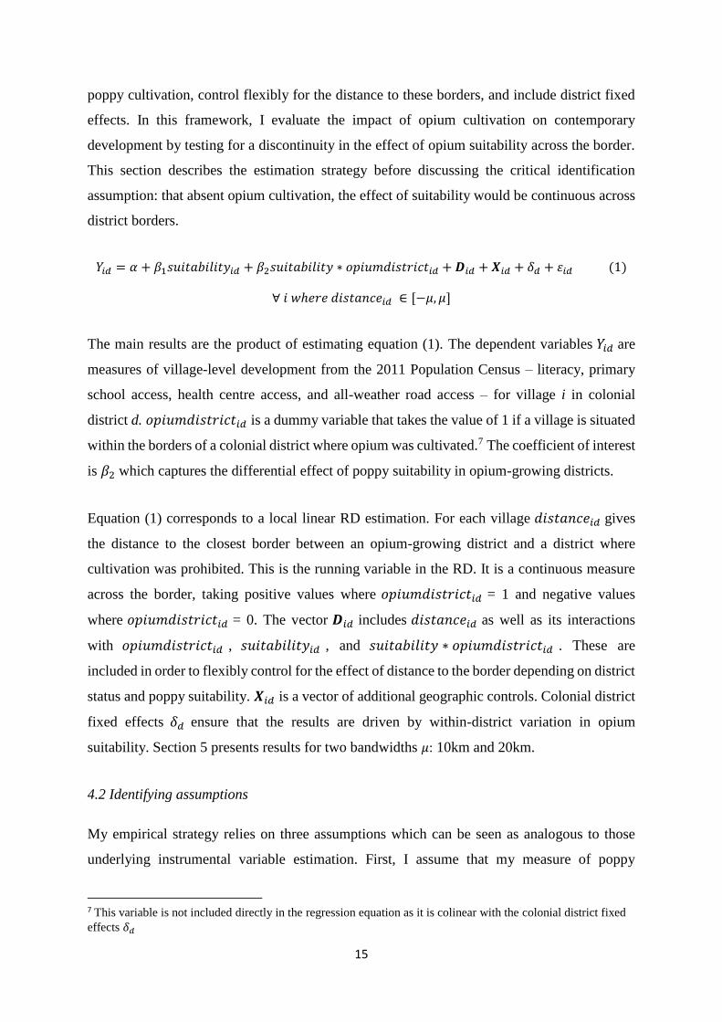
𝑌𝑖𝑑 = 𝛼 + 𝛽1𝑠𝑢𝑖𝑡𝑎𝑏𝑖𝑙𝑖𝑡𝑦𝑖𝑑 + 𝛽2𝑠𝑢𝑖𝑡𝑎𝑏𝑖𝑙𝑖𝑡𝑦 ∗ 𝑜𝑝𝑖𝑢𝑚𝑑𝑖𝑠𝑡𝑟𝑖𝑐𝑡𝑖𝑑 + 𝑫𝑖𝑑 + 𝑿𝑖𝑑 + 𝛿𝑑 + 휀𝑖𝑑 (1)

∀ 𝑖 𝑤ℎ𝑒𝑟𝑒 𝑑𝑖𝑠𝑡𝑎𝑛𝑐𝑒𝑖𝑑 ∈ [−𝜇, 𝜇]

The main results are the product of estimating equation (1). The dependent variables 𝑌𝑖𝑑 are

measures of village-level development from the 2011 Population Census – literacy, primary

school access, health centre access, and all-weather road access – for village i in colonial

district d. 𝑜𝑝𝑖𝑢𝑚𝑑𝑖𝑠𝑡𝑟𝑖𝑐𝑡𝑖𝑑 is a dummy variable that takes the value of 1 if a village is situated

within the borders of a colonial district where opium was cultivated.7 The coefficient of interest

is 𝛽2 which captures the differential effect of poppy suitability in opium-growing districts.

Equation (1) corresponds to a local linear RD estimation. For each village 𝑑𝑖𝑠𝑡𝑎𝑛𝑐𝑒𝑖𝑑 gives

the distance to the closest border between an opium-growing district and a district where

cultivation was prohibited. This is the running variable in the RD. It is a continuous measure

across the border, taking positive values where 𝑜𝑝𝑖𝑢𝑚𝑑𝑖𝑠𝑡𝑟𝑖𝑐𝑡𝑖𝑑 = 1 and negative values

where 𝑜𝑝𝑖𝑢𝑚𝑑𝑖𝑠𝑡𝑟𝑖𝑐𝑡𝑖𝑑 = 0. The vector 𝑫𝑖𝑑 includes 𝑑𝑖𝑠𝑡𝑎𝑛𝑐𝑒𝑖𝑑 as well as its interactions

with 𝑜𝑝𝑖𝑢𝑚𝑑𝑖𝑠𝑡𝑟𝑖𝑐𝑡𝑖𝑑 , 𝑠𝑢𝑖𝑡𝑎𝑏𝑖𝑙𝑖𝑡𝑦𝑖𝑑 , and 𝑠𝑢𝑖𝑡𝑎𝑏𝑖𝑙𝑖𝑡𝑦 ∗ 𝑜𝑝𝑖𝑢𝑚𝑑𝑖𝑠𝑡𝑟𝑖𝑐𝑡𝑖𝑑 . These are

included in order to flexibly control for the effect of distance to the border depending on district

status and poppy suitability. 𝑿𝑖𝑑 is a vector of additional geographic controls. Colonial district

fixed effects 𝛿𝑑 ensure that the results are driven by within-district variation in opium

suitability. Section 5 presents results for two bandwidths 𝜇: 10km and 20km.

4.2 Identifying assumptions

My empirical strategy relies on three assumptions which can be seen as analogous to those

underlying instrumental variable estimation. First, I assume that my measure of poppy

7 This variable is not included directly in the regression equation as it is colinear with the colonial district fixed

effects 𝛿𝑑

16

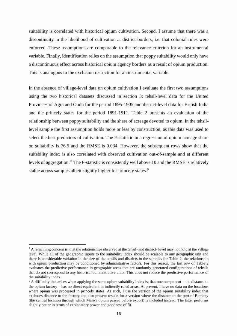
suitability is correlated with historical opium cultivation. Second, I assume that there was a

discontinuity in the likelihood of cultivation at district borders, i.e. that colonial rules were

enforced. These assumptions are comparable to the relevance criterion for an instrumental

variable. Finally, identification relies on the assumption that poppy suitability would only have

a discontinuous effect across historical opium agency borders as a result of opium production.

This is analogous to the exclusion restriction for an instrumental variable.

In the absence of village-level data on opium cultivation I evaluate the first two assumptions

using the two historical datasets discussed in section 3: tehsil-level data for the United

Provinces of Agra and Oudh for the period 1895-1905 and district-level data for British India

and the princely states for the period 1891-1911. Table 2 presents an evaluation of the

relationship between poppy suitability and the share of acreage devoted to opium. In the tehsil-

level sample the first assumption holds more or less by construction, as this data was used to

select the best predictors of cultivation. The F-statistic in a regression of opium acreage share

on suitability is 76.5 and the RMSE is 0.034. However, the subsequent rows show that the

suitability index is also correlated with observed cultivation out-of-sample and at different

levels of aggregation. 8 The F-statistic is consistently well above 10 and the RMSE is relatively

stable across samples albeit slightly higher for princely states.9

8 A remaining concern is, that the relationships observed at the tehsil- and district- level may not hold at the village

level. While all of the geographic inputs to the suitability index should be scalable to any geographic unit and

there is considerable variation in the size of the tehsils and districts in the samples for Table 2, the relationship

with opium production may be conditioned by administrative factors. For this reason, the last row of Table 2

evaluates the predictive performance in geographic areas that are randomly generated configurations of tehsils

that do not correspond to any historical administrative units. This does not reduce the predictive performance of

the suitability index. 9 A difficulty that arises when applying the same opium suitability index is, that one component – the distance to

the opium factory – has no direct equivalent in indirectly ruled areas. At present, I have no data on the locations

where opium was processed in princely states. As such, I use the version of the opium suitability index that

excludes distance to the factory and also present results for a version where the distance to the port of Bombay

(the central location through which Malwa opium passed before export) is included instead. The latter performs

slightly better in terms of explanatory power and goodness of fit.

17

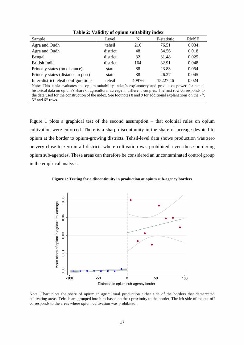
Table 2: Validity of opium suitability index

Sample Level N F-statistic RMSE

Agra and Oudh tehsil 216 76.51 0.034

Agra and Oudh district 48 34.56 0.018

Bengal district 32 31.48 0.025

British India district 164 32.91 0.048

Princely states (no distance) state 88 23.83 0.054

Princely states (distance to port) state 88 26.27 0.045

Inter-district tehsil configurations tehsil 40976 15227.46 0.024 Note: This table evaluates the opium suitability index’s explanatory and predictive power for actual

historical data on opium’s share of agricultural acreage in different samples. The first row corresponds to

the data used for the construction of the index. See footnotes 8 and 9 for additional explanations on the 7th,

5th and 6th rows.

Figure 1 plots a graphical test of the second assumption – that colonial rules on opium

cultivation were enforced. There is a sharp discontinuity in the share of acreage devoted to

opium at the border to opium-growing districts. Tehsil-level data shows production was zero

or very close to zero in all districts where cultivation was prohibited, even those bordering

opium sub-agencies. These areas can therefore be considered an uncontaminated control group

in the empirical analysis.

Figure 1: Testing for a discontinuity in production at opium sub-agency borders

Note: Chart plots the share of opium in agricultural production either side of the borders that demarcated

cultivating areas. Tehsils are grouped into bins based on their proximity to the border. The left side of the cut-off

corresponds to the areas where opium cultivation was prohibited.

18

The estimation strategy outlined above will provide a causal estimate of the effect of opium

production on contemporary outcomes provided that there are no unrelated factors that would

cause poppy suitability to have differential effects across opium agency borders. I conduct

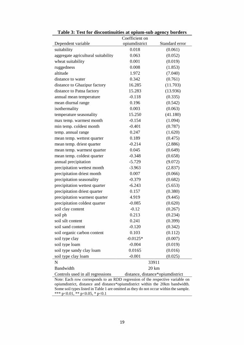
several tests to evaluate the validity of this final assumption. First, I test for discontinuities in

a range of geographic variables at the border (Table 3). Out of 36 variables only one – the share

of soil class clay – exhibits a discontinuity at the 90% significance level. This imbalance is not

inconsistent with chance and I control for the imbalanced variable in subsequent regressions.

Importantly, there is no discontinuity in geographic suitability for poppy cultivation or

aggregate agricultural suitability at former agency borders. Second, I conduct placebo tests

which replicate the estimation of equation (1) but substitute poppy suitability with suitability

for other crops. These crops were not restricted to opium agency borders and so a discontinuous

effect on literacy and public good availability would call the identification strategy into

question. Table 4 shows that no crop exhibits a systematic discontinuity10, which is supporting

evidence that the results in the next section are driven by opium production.

10 Two regressions yield a significant coefficient on the interaction term of interest (health centre on indigo

suitability, and literacy on sugarcane). This number of significant coefficients is not inconsistent with chance and

both suitability indices have no consistent positive or negative effect across other dependent variables.

19

Table 3: Test for discontinuities at opium-sub agency borders

Dependent variable

Coefficient on

opiumdistrict Standard error

suitability 0.018 (0.061)

aggregate agricultural suitability 0.063 (0.052)

wheat suitability 0.001 (0.019)

ruggedness 0.008 (1.853)

altitude 1.972 (7.040)

distance to water 0.342 (0.761)

distance to Ghazipur factory 16.285 (11.703)

distance to Patna factory 15.283 (13.936)

annual mean temperature -0.118 (0.335)

mean diurnal range 0.196 (0.542)

isothermality 0.003 (0.063)

temperature seasonality 15.250 (41.180)

max temp. warmest month -0.154 (1.094)

min temp. coldest month -0.401 (0.787)

temp. annual range 0.247 (1.620)

mean temp. wettest quarter 0.189 (0.475)

mean temp. driest quarter -0.214 (2.886)

mean temp. warmest quarter 0.045 (0.649)

mean temp. coldest quarter -0.348 (0.658)

annual precipitation -5.729 (9.072)

precipitation wettest month -3.963 (2.837)

precipitation driest month 0.007 (0.066)

precipitation seasonality -0.379 (0.682)

precipitation wettest quarter -6.243 (5.653)

precipitation driest quarter 0.157 (0.380)

precipitation warmest quarter 4.919 (9.445)

precipitation coldest quarter -0.085 (0.620)

soil clay content -0.12 (0.267)

soil ph 0.213 (0.234)

soil silt content 0.241 (0.399)

soil sand content -0.120 (0.342)

soil organic carbon content 0.103 (0.112)

soil type clay -0.0125* (0.007)

soil type loam -0.004 (0.019)

soil type sandy clay loam 0.0165 (0.016)

soil type clay loam -0.001 (0.025)

N 33911

Bandwidth 20 km

Controls used in all regressions distance, distance*opiumdistrict Note: Each row corresponds to an RDD regression of the respective variable on

opiumdistrict, distance and distance*opiumdistrict within the 20km bandwidth.

Some soil types listed in Table 1 are omitted as they do not occur within the sample.

*** p<0.01, ** p<0.05, * p<0.1

20

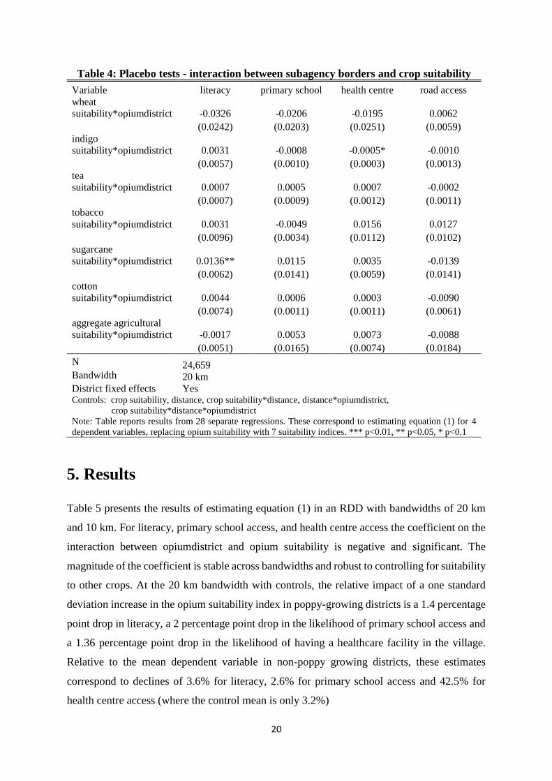
Table 4: Placebo tests - interaction between subagency borders and crop suitability

Variable literacy primary school health centre road access

wheat

suitability*opiumdistrict -0.0326 -0.0206 -0.0195 0.0062

(0.0242) (0.0203) (0.0251) (0.0059)

indigo

suitability*opiumdistrict 0.0031 -0.0008 -0.0005* -0.0010

(0.0057) (0.0010) (0.0003) (0.0013)

tea

suitability*opiumdistrict 0.0007 0.0005 0.0007 -0.0002

(0.0007) (0.0009) (0.0012) (0.0011)

tobacco

suitability*opiumdistrict 0.0031 -0.0049 0.0156 0.0127

(0.0096) (0.0034) (0.0112) (0.0102)

sugarcane

suitability*opiumdistrict 0.0136** 0.0115 0.0035 -0.0139

(0.0062) (0.0141) (0.0059) (0.0141)

cotton

suitability*opiumdistrict 0.0044 0.0006 0.0003 -0.0090

(0.0074) (0.0011) (0.0011) (0.0061)

aggregate agricultural

suitability*opiumdistrict -0.0017 0.0053 0.0073 -0.0088

(0.0051) (0.0165) (0.0074) (0.0184)

N 24,659

20 km

Yes

Bandwidth

District fixed effects Controls: crop suitability, distance, crop suitability*distance, distance*opiumdistrict,

crop suitability*distance*opiumdistrict

Note: Table reports results from 28 separate regressions. These correspond to estimating equation (1) for 4

dependent variables, replacing opium suitability with 7 suitability indices. *** p<0.01, ** p<0.05, * p<0.1

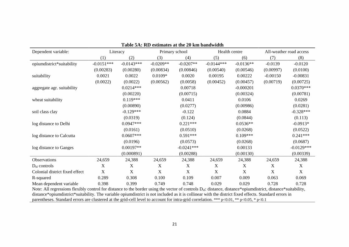
5. Results

Table 5 presents the results of estimating equation (1) in an RDD with bandwidths of 20 km

and 10 km. For literacy, primary school access, and health centre access the coefficient on the

interaction between opiumdistrict and opium suitability is negative and significant. The

magnitude of the coefficient is stable across bandwidths and robust to controlling for suitability

to other crops. At the 20 km bandwidth with controls, the relative impact of a one standard

deviation increase in the opium suitability index in poppy-growing districts is a 1.4 percentage

point drop in literacy, a 2 percentage point drop in the likelihood of primary school access and

a 1.36 percentage point drop in the likelihood of having a healthcare facility in the village.

Relative to the mean dependent variable in non-poppy growing districts, these estimates

correspond to declines of 3.6% for literacy, 2.6% for primary school access and 42.5% for

health centre access (where the control mean is only 3.2%)

21

Table 5A: RD estimates at the 20 km bandwidth

Dependent variable: Literacy Primary school Health centre All-weather road access

(1) (2) (3) (4) (5) (6) (7) (8)

opiumdistrict*suitability -0.0151*** -0.0143*** -0.0209** -0.0207** -0.0144*** -0.0136** -0.0139 -0.0120

(0.00283) (0.00280) (0.00834) (0.00846) (0.00540) (0.00546) (0.00997) (0.0100)

suitability 0.0021 0.0022 0.0109* 0.0020 0.00195 0.00222 -0.00150 -0.00831

(0.0022) (0.0022) (0.00562) (0.0058) (0.00452) (0.00457) (0.00719) (0.00725)

aggregate agr. suitability 0.0214*** 0.00718 -0.000201 0.0370***

(0.00220) (0.00715) (0.00324) (0.00781)

wheat suitability 0.119*** 0.0411 0.0106 0.0269

(0.00890) (0.0277) (0.00986) (0.0281)

soil class clay -0.129*** -0.122 0.0884 -0.328***

(0.0319) (0.124) (0.0844) (0.113)

log distance to Delhi 0.0947*** 0.221*** 0.0536** -0.0913*

(0.0161) (0.0510) (0.0268) (0.0522)

log distance to Calcutta 0.0607*** 0.591*** 0.109*** 0.241***

(0.0196) (0.0573) (0.0268) (0.0687)

log distance to Ganges 0.00197** -0.0241*** 0.00133 -0.0129***

(0.000891) (0.00288) (0.00130) (0.00339)

Observations 24,659 24,388 24,659 24,388 24,659 24,388 24,659 24,388

Did controls X X X X X X X X

Colonial district fixed effect X X X X X X X X

R-squared 0.289 0.308 0.100 0.109 0.007 0.009 0.063 0.069

Mean dependent variable 0.398 0.399 0.749 0.748 0.029 0.029 0.728 0.728

Note: All regressions flexibly control for distance to the border using the vector of controls Did: distance, distance*opiumdistrict, distance*suitability,

distance*opiumdistrict*suitability. The variable opiumdistrict is not included as it is collinear with the district fixed effects. Standard errors in

parentheses. Standard errors are clustered at the grid-cell level to account for intra-grid correlation. *** p<0.01, ** p<0.05, * p<0.1

22

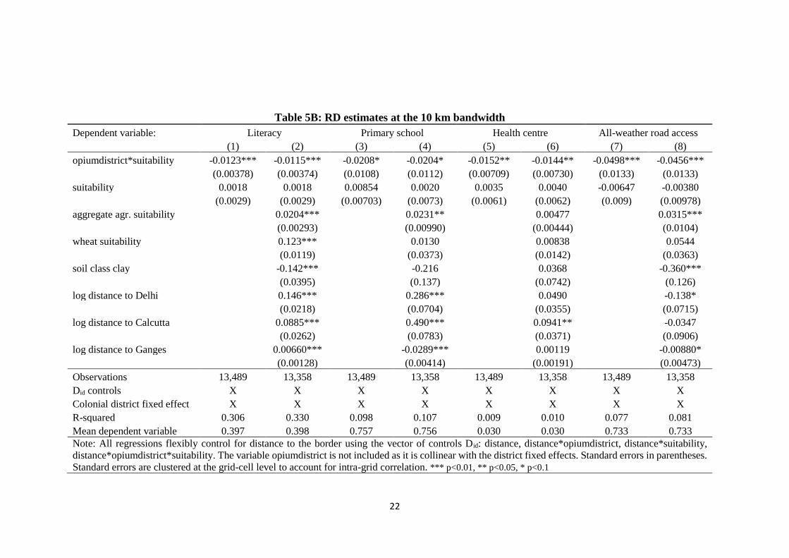
Table 5B: RD estimates at the 10 km bandwidth

Dependent variable: Literacy Primary school Health centre All-weather road access

(1) (2) (3) (4) (5) (6) (7) (8)

opiumdistrict*suitability -0.0123*** -0.0115*** -0.0208* -0.0204* -0.0152** -0.0144** -0.0498*** -0.0456***

(0.00378) (0.00374) (0.0108) (0.0112) (0.00709) (0.00730) (0.0133) (0.0133)

suitability 0.0018 0.0018 0.00854 0.0020 0.0035 0.0040 -0.00647 -0.00380

(0.0029) (0.0029) (0.00703) (0.0073) (0.0061) (0.0062) (0.009) (0.00978)

aggregate agr. suitability 0.0204*** 0.0231** 0.00477 0.0315***

(0.00293) (0.00990) (0.00444) (0.0104)

wheat suitability 0.123*** 0.0130 0.00838 0.0544

(0.0119) (0.0373) (0.0142) (0.0363)

soil class clay -0.142*** -0.216 0.0368 -0.360***

(0.0395) (0.137) (0.0742) (0.126)

log distance to Delhi 0.146*** 0.286*** 0.0490 -0.138*

(0.0218) (0.0704) (0.0355) (0.0715)

log distance to Calcutta 0.0885*** 0.490*** 0.0941** -0.0347

(0.0262) (0.0783) (0.0371) (0.0906)

log distance to Ganges 0.00660*** -0.0289*** 0.00119 -0.00880*

(0.00128) (0.00414) (0.00191) (0.00473)

Observations 13,489 13,358 13,489 13,358 13,489 13,358 13,489 13,358

Did controls X X X X X X X X

Colonial district fixed effect X X X X X X X X

R-squared 0.306 0.330 0.098 0.107 0.009 0.010 0.077 0.081

Mean dependent variable 0.397 0.398 0.757 0.756 0.030 0.030 0.733 0.733

Note: All regressions flexibly control for distance to the border using the vector of controls Did: distance, distance*opiumdistrict, distance*suitability,

distance*opiumdistrict*suitability. The variable opiumdistrict is not included as it is collinear with the district fixed effects. Standard errors in parentheses.

Standard errors are clustered at the grid-cell level to account for intra-grid correlation. *** p<0.01, ** p<0.05, * p<0.1

23

The results for all-weather road access are less conclusive. The coefficient is negative

throughout, but only significant at the 10 km bandwidth, where it also larger in magnitude.

Appendix Table 1 presents the results for a separate measure of infrastructure that could

potentially be more prevalent in poppy-cultivating areas as a result of opium production:

irrigation. While critics of the opium trade claimed that the system of advance payments led to

indebtedness by farmers or the appropriation of the advance by village headmen, its proponents

argued that they allowed farmers to make investments required for poppy cultivation – in

particular in wells for irrigation (Allen 1852, Richards 1981). Using 2011 census data on the

share of agricultural land that is irrigated, and the share that is irrigated by wells, I find no

evidence of a positive lasting impact on irrigation. Instead, the coefficients are negative and

significant.

It is important to note that these estimates are local average treatment effects which may not

be representative for the entire opium-growing region. Given the empirical design, there are

two reasons to question the validity of extrapolating from the results. Firstly, as with any RDD,

the restriction of the sample to narrow bandwidths around opium sub-agency borders implies

that it may not be representative of villages far from the border. Secondly, the opium suitability

index only explains part of the variation in actual opium cultivation – a characteristic common

to instrumental variables – which again implies that the results should be interpreted as a LATE.

6. Mechanisms

A natural starting point for explaining persistent effects on contemporary measures of

education and healthcare is to assess colonial policy in these sectors. Using data on public

expenditure between 1895 and 1905 from the district gazetteers of Agra and Oudh, I test

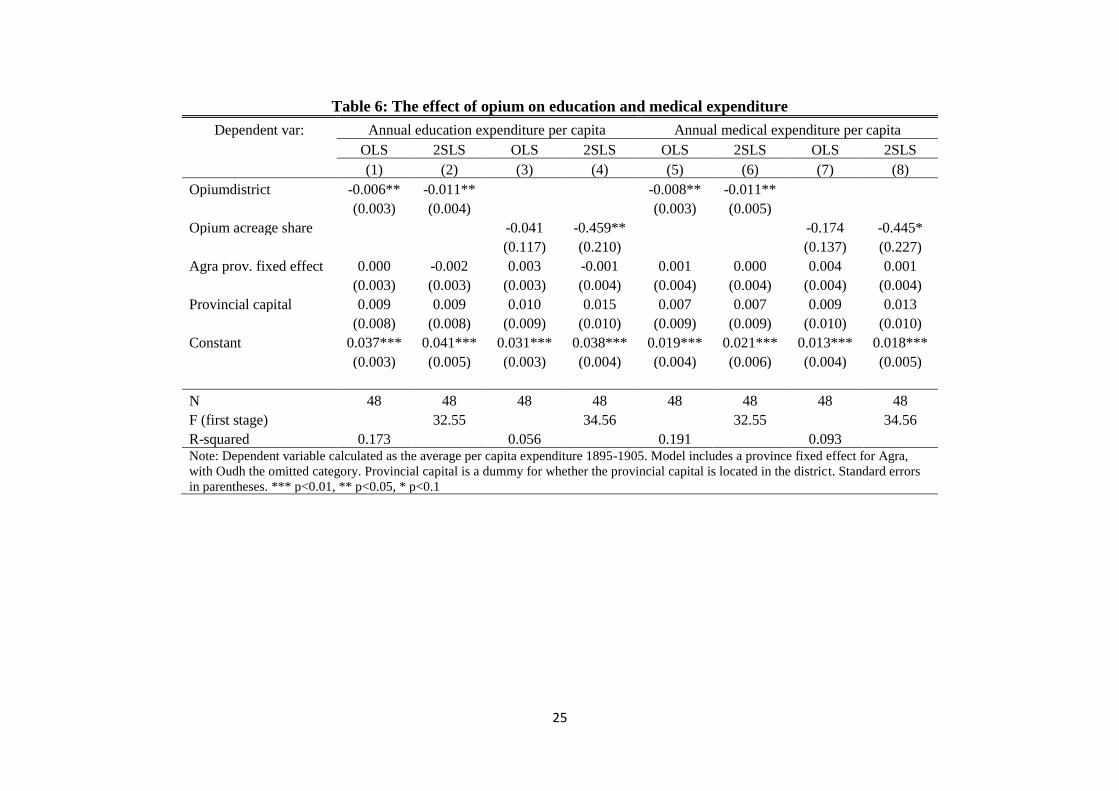
whether opium cultivation led to shaped government spending patterns. Table 6 provides OLS

estimates (columns 1, 3, 5 and 7) for the effect of (i) being an opium district and (ii) the opium

share of agricultural acreage on per capita spending on education and health. Given the likely

endogeneity of these variables, I instrument for them using the opium suitability index

(columns 2, 4, 6 and 8). All 2SLS results show a significant negative effect of opium production

on education and health expenditure. Given the small sample size (48 districts) these results

are only suggestive. They are however, consistent with the explanation that current differences

in the availability of public goods are rooted in opium-era policies.

24

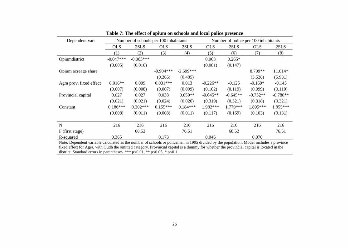
Further supporting evidence comes from slightly larger datasets at the tehsil-level. Table 7

replicates the previous analysis for different dependent variables: the number of schools per

capita and the number of policemen per capita. Again, the results indicate that opium

production was detrimental for human capital provision, with a significant negative effect on

the number of schools in all specifications. By contrast columns (5) to (8) show a positive and

significant effect on the strength of the police force. This result is in line with Deshpande’s

(2009) claim that the British Government sought to maintain a large security presence in

opium-cultivating areas to enforce the monopsony and curtail smuggling.

25

Table 6: The effect of opium on education and medical expenditure

Dependent var: Annual education expenditure per capita Annual medical expenditure per capita

OLS 2SLS OLS 2SLS OLS 2SLS OLS 2SLS

(1) (2) (3) (4) (5) (6) (7) (8)

Opiumdistrict -0.006** -0.011** -0.008** -0.011**

(0.003) (0.004) (0.003) (0.005)

Opium acreage share -0.041 -0.459** -0.174 -0.445*

(0.117) (0.210) (0.137) (0.227)

Agra prov. fixed effect 0.000 -0.002 0.003 -0.001 0.001 0.000 0.004 0.001

(0.003) (0.003) (0.003) (0.004) (0.004) (0.004) (0.004) (0.004)

Provincial capital 0.009 0.009 0.010 0.015 0.007 0.007 0.009 0.013

(0.008) (0.008) (0.009) (0.010) (0.009) (0.009) (0.010) (0.010)

Constant 0.037*** 0.041*** 0.031*** 0.038*** 0.019*** 0.021*** 0.013*** 0.018***

(0.003) (0.005) (0.003) (0.004) (0.004) (0.006) (0.004) (0.005)

N 48 48 48 48 48 48 48 48

F (first stage) 32.55 34.56 32.55 34.56

R-squared 0.173 0.056 0.191 0.093 Note: Dependent variable calculated as the average per capita expenditure 1895-1905. Model includes a province fixed effect for Agra,

with Oudh the omitted category. Provincial capital is a dummy for whether the provincial capital is located in the district. Standard errors

in parentheses. *** p<0.01, ** p<0.05, * p<0.1

26

Table 7: The effect of opium on schools and local police presence

Dependent var: Number of schools per 100 inhabitants Number of police per 100 inhabitants

OLS 2SLS OLS 2SLS OLS 2SLS OLS 2SLS

(1) (2) (3) (4) (5) (6) (7) (8)

Opiumdistrict -0.047*** -0.063*** 0.063 0.265*

(0.005) (0.010) (0.081) (0.147) Opium acreage share -0.904*** -2.599*** 8.709** 11.014*

(0.265) (0.485) (3.528) (5.931)

Agra prov. fixed effect 0.016** 0.009 0.031*** 0.013 -0.226** -0.125 -0.169* -0.145

(0.007) (0.008) (0.007) (0.009) (0.102) (0.119) (0.099) (0.110)

Provincial capital 0.027 0.027 0.038 0.059** -0.645** -0.645** -0.752** -0.780**

(0.021) (0.021) (0.024) (0.026) (0.319) (0.321) (0.318) (0.321)

Constant 0.186*** 0.202*** 0.155*** 0.184*** 1.982*** 1.779*** 1.895*** 1.855***

(0.008) (0.011) (0.008) (0.011) (0.117) (0.169) (0.103) (0.131)

N 216 216 216 216 216 216 216 216

F (first stage) 68.52 76.51 68.52 76.51

R-squared 0.365 0.173 0.046 0.070 Note: Dependent variable calculated as the number of schools or policemen in 1905 divided by the population. Model includes a province

fixed effect for Agra, with Oudh the omitted category. Provincial capital is a dummy for whether the provincial capital is located in the

district. Standard errors in parentheses. *** p<0.01, ** p<0.05, * p<0.1

27

Finally, I evaluate whether the same negative relationship between poppy cultivation and

present-day outcomes holds in areas that were formerly princely states. If so, one might

conclude that the adverse effects of opium stemmed from its use as a narcotic, rather than the

institutions and policies specific to British state-run opium production. In the absence of the

geographic boundaries imposed by the British, I cannot replicate the RDD analysis. Appendix

Table 2 therefore presents reduced form estimates for a sample of 36,578 villages in 40 princely

states which had positive opium cultivation. I include princely state fixed effects and test

whether opium suitability explains within-state variation in literacy or public good provision.

I find no evidence of a negative impact. For all dependent variables the coefficient is positive

and insignificant. Unfortunately, these results are not directly comparable to those in Table 5

and are less well-identified. The absence of an effect in areas not under direct British rule is

consistent with the explanation presented in this section but is not conclusive.

7. Conclusion

The parts of Bihar, Jharkhand, and Uttar Pradesh where opium was produced under British

rule, lag behind much of India in terms of income, literacy, and access to public goods. This

paper provides evidence to suggest that the state-run extraction of opium rents causally

contributed to these regions’ current comparative underdevelopment. Using an RDD design

that exploits the interaction between geographic suitability for poppy cultivation and

administrative boundaries that confined production to specific areas, I show that the opium

industry had persistent negative effects on local development. Villages with a higher likelihood

of historical opium cultivation have lower literacy, and less access to private schools and

healthcare facilities. There is no evidence that opium cultivation gave rise to persistent benefits

in terms of access to roads or irrigation infrastructure. Instead, historical administrative data

suggest that British officials in poppy-growing districts invested less in education and health,

while spending more on a police force that could help to secure the opium monopsony and

combat smuggling. Colonial opium production in India might therefore be considered an

example of a historical resource curse. Its adverse effects on the wider economy have persisted

long after the opium agencies were closed.

28

References

Acemoglu, Daron, Simon Johnson, and James A. Robinson. "The colonial origins of

comparative development: An empirical investigation." American economic review 91, no. 5

(2001): 1369-1401.

Acemoglu, Daron, Simon Johnson, and James A. Robinson. "Reversal of fortune: Geography

and institutions in the making of the modern world income distribution." The Quarterly journal

of economics 117, no. 4 (2002): 1231-1294.

Allen, Nathan. The opium trade: including a sketch of its history, extent, effects, etc., as carried

on in India and China. JP Walker, 1853.

Banerjee, Abhijit, and Lakshmi Iyer. "History, institutions, and economic performance: The

legacy of colonial land tenure systems in India." American economic review 95, no. 4 (2005):

1190-1213.

Belloni, Alexandre, and Victor Chernozhukov. "Least squares after model selection in high-

dimensional sparse models." Bernoulli 19, no. 2 (2013): 521-547.

Caselli, Francesco, and Tom Cunningham. "Leader behaviour and the natural resource

curse." Oxford Economic Papers 61, no. 4 (2009): 628-650

Dell, Melissa. "The persistent effects of Peru's mining mita." Econometrica 78, no. 6 (2010):

1863-1903.

Dell, Melissa, and Benjamin A. Olken. "The Development Effects of the Extractive Colonial

Economy: The Dutch Cultivation System in Java." (2017).

Deshpande, Anirudh. "An Historical Overview of Opium Cultivation and Changing State

Attitudes towards the Crop in India, 1878–2000 AD." Studies in History 25, no. 1 (2009): 109-

143.

Engerman, Stanley L., and Kenneth L. Sokoloff. "Factor endowments, institutions, and

differential paths of growth among new world economies." How Latin America Fell Behind

(1997): 260-304.

Fick, Stephen E., and Robert J. Hijmans. "WorldClim 2: new 1‐km spatial resolution climate

surfaces for global land areas." International Journal of Climatology 37, no. 12 (2017): 4302-

4315.

29

Frankel, Jeffrey A. The natural resource curse: a survey. No. w15836. National Bureau of

Economic Research, 2010.

Haq, M. Drugs in South Asia: From the opium trade to the present day. Springer, 2000.

Hijmans, R. J., L. Guarino, and P. Mathur. "Diva-GIS version 7.5." Manual. www. diva-gis.

org (2012).

Iyer, Lakshmi. "Direct versus indirect colonial rule in India: Long-term consequences." The

Review of Economics and Statistics 92, no. 4 (2010): 693-713.

Kienberger, Stefan, Raphael Spiekermann, Dirk Tiede, Irmgard Zeiler, and Coen Bussink.

"Spatial risk assessment of opium poppy cultivation in Afghanistan: integrating environmental

and socio-economic drivers." International Journal of Digital Earth 10, no. 7 (2017): 719-736.

Lowes, Sara, and Eduardo Montero. Blood Rubber: The Effects of Labor Coercion on

Institutions and Culture in the DRC. Working paper, Harvard, http://www. saralowes.

com/research. html, 2016.

Richards, John F. "The Indian empire and peasant production of opium in the nineteenth

century." Modern Asian Studies 15, no. 1 (1981): 59-82.

Richards, John F. "Opium and the British Indian Empire: The Royal Commission of

1895." Modern Asian Studies 36, no. 2 (2002): 375-420.

Ross, Michael L. "The political economy of the resource curse." World politics 51, no. 2

(1999): 297-322.

Ross, Michael. "The natural resource curse: How wealth can make you poor." Natural

resources and violent conflict: options and actions (2003): 17-42.

Sahu, A. C. "Genesis and Growth of Indo-Chinese Opium Monopoly under East India

Company." In Proceedings of the Indian History Congress, vol. 38, pp. 529-533. Indian

History Congress, 1977.

Sala-i-Martin, Xavier, and Arvind Subramanian. "Addressing the natural resource curse: An

illustration from Nigeria." Journal of African Economies 22, no. 4 (2013): 570-615.

Shaver, Andrew, David B. Carter, and Tsering Wangyal Shawa. "Terrain ruggedness and land

cover: Improved data for most research designs." Conflict Management and Peace

Science (2016): 0738894216659843.

30

Watt, George. A dictionary of the economic products of India. Vol. 6. Superintendent of

Government Printing, 1892.

Wright, Harold RC. "The Emancipation of the Opium Cultivators in Benares." International

Review of Social History, no. 3 (1959): 446-460.