The History of the Cross Section of Stock

Returns∗

Juhani T. Linnainmaa Michael R. Roberts

June 2017 (Draft)

Abstract

Using data spanning the 20th century, we show that the majority of accounting-based

return anomalies, including investment and profitability, are most likely an artifact of

data snooping. When examined out-of-sample by moving either backward or forward in

time, most anomalies’ average returns and Sharpe ratios decrease, while their volatilities

and correlations with other anomalies increase. The data-snooping problem is so severe

that even the true asset pricing model is expected to be rejected when tested using in-

sample data. The few anomalies that do persist out-of-sample correlate with the shift

from investment in physical capital to intangible capital, and the increasing reliance on

debt financing observed over the 20th century. Our results emphasize the importance

of validating asset pricing models out-of-sample, question the extent to which investors

learn of mispricing from academic research, and highlight the linkages between anomalies

and economic fundamentals.

∗Juhani Linnainmaa is with the University of Southern California and NBER and Michael Roberts is withthe Wharton School of the University of Pennsylvania and NBER. We thank Jules van Binsbergen, MikeCooper (discussant), Ken French, Chris Hrdlicka (discussant), Travis Johnson (discussant), Mark Leary, JonLewellen (discussant), David McLean, Toby Moskowitz, Robert Novy-Marx, Christian Opp, Jeff Pontiff, NickRoussanov, and Rob Stambaugh for helpful discussions, and seminar and conference participants at CarnegieMellon University, Georgia State University, Northwestern University, University of Lugano, University ofCopenhagen, University of Texas at Austin, American Finance Association 2017, NBER Behavioral Finance2017, SFS 2016 Finance Cavalcade, and Western Finance Association 2016, meetings for valuable comments.

1 Introduction

An “anomaly” in the context of financial economics typically refers to the rejection of an

asset pricing model, such as the capital asset pricing model (CAPM) or the three-factor

model of Fama and French (1993). Academic research has uncovered a large number of such

anomalies—314 according to Harvey, Liu, and Zhu (2015) with the majority being identified

during the last 15 years.

For each hypothesis test resulting in rejection of a particular model there is a test size

quantifying the probability of a false rejection, i.e., Type I error. While the test size for any

one test is low, often 5%, test size grows quickly with the number of tests (e.g., Bickel and

Doksum (1977)). Multiple comparison methods exist to address this issue (e.g., White (2000))

but these methods rely on the reporting of all tests to adjust test sizes and p-values. Because

there is no mechanism to ensure authors report all hypothesis tests in published papers, let

alone unpublished papers, statistical solutions have their limitations.

To understand these limitations and identify the mechanisms behind observed anomalies,

we perform an out-of-sample analysis by gathering comprehensive accounting data extending

back to the start of the 20th century. More precisely, we merge data collected from Moody’s

manuals between 1918 and 1970 with Standard & Poor’s (S&P) Compustat database and

the Center for Research in Security Prices (CRSP). The result is comprehensive coverage of

returns and accounting information - balance sheet and income statement data - from 1926

to 2016.

After performing a number of tests aimed at ensuring the quality of the Moody’s data, we

investigate the behavior of accounting-based anomalies across three eras encompassed by our

data:

1. “in-sample” denotes the sample frame used in the original discovery of an anomaly (e.g.,

1970 to 2004),

2. “pre-sample” denotes the sample frame occurring prior to the in-sample period (e.g.,

1926 to 1969), and

1

3. “post-sample” denotes the sample frame occurring after the in-sample period (e.g., 2005

to 2016).

Each anomaly we study spans these three eras, though the start and end dates for each era

will vary by anomaly.

The breadth of our sample frame enables us to examine competing explanations for the ex-

istence of these anomalies based on (1) unmodeled risk, (2) mispricing, and (3) data-snooping.

Each of these mechanisms generate different testable implications across different time-periods

encompassed by our sample. By studying variation in anomaly behavior across different sub-

samples, we are able to better understand the role of each mechanism.

To illustrate our empirical approach and broader findings, we first characterize the return

behavior of the profitability and investment factors during the pre-sample period — 1926 to

1962 for both. Our focus on these factors is motivated by findings in Fama and French (2015,

2017) and Hou, Xue, and Zhang (2015) showing their importance, in combination with the

market and size factors, for capturing cross-sectional variation in stock returns.

We find no economically or statistically significant premiums on the profitability and in-

vestment factors in the pre-sample period, during which the average returns are negative one

(t-value = -0.06) and six (t-value = 0.64) basis points (bps) per month, respectively. The

CAPM the alphas are 17 (t-value = 1.11) and three (t-value = 0.33) bps per month. The

Fama and French (1993) three-factor model alphas are 22 (t-value = 1.66) and -2 (t-value =

−0.25) bps per month. These results stand in stark contrast to those found with in-sample

data where profitability and investment factors average a statistically significant 27 and 40

bps per month, and the corresponding CAPM and three-factor alphas are similarly significant.

The investment and profitability premium attenuation in the pre-sample data is represen-

tative of most of the other anomalies that we examine. Twenty eight of the 36 anomalies we

study earn average returns that are statistically insignificant during the pre-sample period.

Twenty eight CAPM alphas and and 20 of the three factor model alphas are statistically

insignificant as well.

This insignificance is unlikely due to low power. For most anomalies, the pre-sample

2

period is 37 years long, typically longer than the original study’s sample period. Additionally,

average returns, Sharpe ratios, CAPM and three-factor model alphas and information ratios

(i.e., alpha scaled by residual standard deviation), all decrease sharply, between 50% and 70%,

while the partial correlation between each anomaly and other anomalies increases from 0.06 to

0.56. The post-sample results are similar, consistent with the findings in McLean and Pontiff

(2016).

We also find that the choice of in-sample start date is particularly important for the

significance of an anomaly. By exploiting the asynchronicity of the in-sample start dates

across anomalies, we show that the rise of anomalies does not coincide with a specific time

period or economic event. Rather, anomalies are present only during the precise window in

which they were originally discovered. Small perturbations to the in-sample start date of each

anomaly lead to significant reductions, ranging from 50% to 75%, in the average return and

alphas.

In total, our results show that the anomalous behavior of most anomalies is a decidedly

in-sample phenomenon, consistent with data-snooping. In addition to large excess returns, we

find low in-sample volatilities that correlate positively with those returns. Coupled with low

correlations among the anomalies, t-values from multivariate regressions tend to be inflated

in-sample.

In contrast, explanations based on mispricing and unmodeled risk face several challenges

in reconciling our results. Most frictions responsible for limits to arbitrage (e.g., transac-

tion costs, liquidity, information availability) have declined over the last century (Jones 2002;

French 2008; Hasbrouck 2009). Even if this decline has not been constant, the nonmono-

tonicity of our results and variation across characteristics requires an explanation based on

transient fads for those anomalies that do not persist, and seemingly permanent fads for those

that do.

Perhaps more challenging is the sensitivity of anomalies to the precise sample start date.

To reconcile these findings, one must rely on structural breaks in the risks that investors care

about, or transient fads that occur on an almost annual basis and and operate through a

3

variety of different accounting signals.

What data-snooping does not explain is the few anomalies that persist out-of-sample.

While a complete investigation into the economic mechanisms behind these surviving anoma-

lies is beyond the scope of this study, they do exhibit interesting temporal variation in light of

broader economic changes. In the pre-sample period, significant anomalies are based on: real

investment (inventory or capital), financial distress, accounting returns (equity and assets),

and equity financing. In the post-sample period, financial distress and accounting returns re-

main significant but real investment and equity financing do not. Instead, income statement

measures (e.g., sales and earnings) and the total amount of external financing are signifi-

cant. This shift coincides with the shift away from tangible to intangible capital investment

(Bond, Cummins, Eberly, and Shiller 2000), and the growing importance of debt as a source

of financing (Graham, Leary, and Roberts 2015).

A number of studies exploit out-of-sample testing strategies to investigate anomalies. Sev-

eral studies examine anomalies in domestic equity markets by exploiting sample periods prior

to (e.g., Jaffe, Keim, and Westerfield (1989) and Wahal (2016)) or after (e.g,. Jegadeesh and

Titman (2001), Schwert (2003), Chordia, Subrahmanyam, and Tong (2014), and McLean and

Pontiff (2016)) the original sample period used to discover the anomaly. Other studies have

used international markets (Fama and French 1998), other asset classes (Asness, Moskowitz,

and Pedersen 2013), and other securities (Barber and Lyon 1997) as out-of-sample tests. What

distinguishes our study is (1) its breadth, which enables us to better gauge the extent of po-

tential data-snooping, and (2) the combination of pre- and post-sample data, which provides

for more powerful tests of competing hypotheses and a richer set of results to guide future

work.

Other studies explore the statistical implications of data snooping for anomalous returns

(e.g., Lo and MacKinlay (1990), Sullivan, Timmermann, and White (1999, 2001), Harvey, Liu,

and Zhu (2015), and Yan and Zheng (2017)). Our study compliments these by providing a

useful benchmark against which in-sample statistical corrections can be compared. When we

apply the t-values corrected for multiple comparisons, as proposed by Harvey, Liu, and Zhu

4

(2015), we find 17 significant Fama-French three-factor model alphas compared to 16 found

in the pre-sample period. More interesting, ten anomalies are in the intersection of these two

sets of robust anomalies. Thus, while statistical corrections may provide a greater degree

of reassurance that one’s findings are not a statistical artifact, they cannot replace the new

information obtained from out-of-sample data.

2 Data

2.1 Data sources

We use data from four sources. First, we obtain monthly stock returns and shares-outstanding

data from the Center for Research in Securities Prices (CRSP) database from January 1926

through December 2016. We exclude securities other than common stocks (share codes 10 and

11). CRSP includes all firms listed on the New York Stock Exchange (NYSE) since December

1925, all firms listed on the American Stock Exchange (AMEX) since 1962, and all firms listed

on the NASDAQ since 1972. We take delisting returns from CRSP; if a delisting return is

missing and the delisting is performance-related, we impute a return of −30% for NYSE and

Amex firms (Shumway 1997) and −55% for Nasdaq firms (Shumway and Warther 1999).

Second, we take annual accounting data from Standard and Poor’s Compustat database.

This data begins in 1947 for some firms, but become more comprehensive in 1962. Standard

and Poor’s established Compustat in 1962 to serve the needs of financial analysts, and back-

filled information only for those firms that were deemed to be of the greatest interest to these

analysts (Ball and Watts 1977). The result is significantly sparser coverage prior to 1963 for

a selected sample of good-performing firms.

Third, we add accounting data from Moody’s Industrial and Railroad manuals (Moody’s).

We collect information for all CRSP firms going back to 1918. These same data have previously

been used in Graham, Leary, and Roberts (2014, 2015). These data do not include financials

or utilities.

Fourth, we add to our data the historical book value of equity data provided by Ken French.

5

These are the data initially collected by Davis, Fama, and French (2000) for industrial firms,

but later expanded to include non-industrial firms. We use the same definition of book value

of equity as Fama and French (1992) throughout this study.

In constructing our final database, we make the conventional assumption that accounting

data are available six months after the end of the fiscal year (Fama and French 1993). In

most of our analyses, we construct factors using annual rebalancing. When we sort stocks

into portfolios at the end of June in year t, we therefore use accounting information from the

fiscal year that ended in year t− 1.

Detailed discussions of the data and variable construction are contained in the appendix.

2.2 Firm coverage

Table 1 shows the number of firms in the CRSP database at five years intervals from 1925

through 1965. The number of CRSP firms increases over time from 490 n 1925 to 1,113 in

1960. The large jump to 2,164 firms in 1965 is due to the inclusion of AMEX-listed firms

in 1962. Because Moody’s does not cover financials and utilities, we exclude these firms

henceforth except when mentioned otherwise. The number of nonfinancials and nonutilities

on CRSP increases from 458 to 1,905 from 1925 through 1965.

The third line shows the number of firms for which Compustat provides any accounting

information. There is no information until 1947, and by 1950 the data are available for 313 of

the 881 NYSE nonfinancials and nonutilities. By 1965, which is the date by which Compustat

is survivorship-bias free, the accounting data are available 59% of firms. The fourth line shows

that when we add Moody’s to Compustat, we get a marked increase in coverage before and

after 1965. At the start of CRSP in 1925, Moody’s coverage is approximately 75%. In 1965,

when Compustat is free of backfill bias, coverage of CRSP firms increases from 59% with

Compsutat alone to 74%.

Figure 1 presents a visual representation of these coverage patterns throughout our entire

sample. The figure highlights the increased coverage coming with Moody’s data through 1970.

It also reveals consistent coverage of CRSP, but for the years immediately after the addition

6

of AMEX and NASDAQ firms.1

The lower part of Table 1 shows that coverage varies significantly by data item in the

Pre-1965 era. This coverage variation reflects coarser data in the earlier parts of the sample

due to greater discretion of what firms reported to Moody’s. That said, coverage of balance

sheet data is near 100% for most major accounts throughout the sample period, and income

statement coverage improves quickly after 1930.

2.3 Data quality

We perform several tests to gauge the quality of the Moody’s data and ensure its consistency

with more recent Compustat data. These tests compliment those performed by Graham,

Leary, and Roberts (2015). To conserve space, the results discussed in this section are not

tabulated.

We first note that the Securities Exchange Act of 1934 was enacted in 1934 to ensure

the flow of accurate and systematic accounting information. Cohen, Polk, and Vuolteenaho

(2003), discuss the Act in detail and, based on their analysis of the historical SEC enforcement

records, determine that post-1936 accounting data is of sufficiently high quality to employ in

empirical analysis. They characterize the first two years after the enactment of the act as an

initial enforcement period, and drop these years from their sample. Although our data start

in 1926 for many anomalies, we repeat all of our analysis excluding pre-1936 data. We discuss

some results in the body but relegate the rest to an appendix.2

Second, we compare the extent to which the accounting data from pre- and post-1963

conform to clean-surplus accounting. Under clean-surplus accounting, the change in assets

and liabilities must pass through the income statement, implying that the change in book

value of equity equals earnings minus dividends (Ohlson 1995). Mathematically, this relation

1We exclude year 2016 from this graph because, as of the time this study was undertaken, most firms’accounting information was not yet available for the fiscal year that ended in 2016.

2Cohen, Polk, and Vuolteenaho (2003) also note that the pre-1936 data are congruent with the later data:“It is comforting, however, that our main regression results are robust to the choice between the 1928–1997and 1936–1997 periods.” The timing convention in Cohen, Polk, and Vuolteenaho (2003) is such that theiryear 1936 observations use book values from 1937. In our subsample analysis, we start the return data in July1938 so that, consistent with Cohen, Polk, and Vuolteenaho (2003), the book values of equity come from 1937.

7

can be expressed as

Clean-surplus ROEt = log

{(1 +Rt)×MEt−1 −Dt

MEt

× BEt

BEt−1−

[1− Dt

BEt−1

]}, (1)

where Rt is the total stock return over fiscal year t, MEt and BEt are the market and book

values of equity at the end of fiscal year t, and Dt is the sum of dividends paid over fiscal year

t.3

We test this relation by estimating panel regressions of clean-surplus ROE on reported

ROE using annual data,

Clean-surplus ROEit = b1Reported ROEit+b2Postt+b3Postt×Reported ROEit+µi+εit, (2)

where µi are firm fixed effects and Postt identifies post-1963 data. This regression measures

how closely clean-surplus ROE tracks reported ROE before and after 1963.

Under the null that firms adhere to clean-surplus accounting, the slope coefficient on

reported profitability is equal to one. We note that a test of conformity to clean-surplus

accounting is a joint test of two hypotheses: k (a) errors in Moody’s manuals, and (b) firms’

tendencies to circumvent the income statement. Even under the generally accepted accounting

principles (GAAP), some transactions can circumvent the income statement and affect the

book value of equity directly.4 So, real-world income statement and balance sheet information

rarely line up exactly as they should under this ideal.

The results, not tabulated, reveal that the pre-1963 slope on Reported ROE is 1.04 (SE =

0.06). The interaction between Postt and Reported ROE is −0.32 (SE = 0.06), implying that

the post-1963 slope on reported ROE is 0.71. (The standard errors (SE) are clustered by year.)

The difference in slopes shows that clean-surplus accounting is violated more frequently in the

more recent data, most likely due to an increase in transactions that circumvent this relation.

3This formula adjusts the change in the book value of equity for dividends, share repurchases, and shareissuances to back out the implied earnings. The income-statement profitability is the net income reported forfiscal year t divided by the book value of equity at the end of fiscal year t− 1. See, for example, Vuolteenaho(2002), Cohen, Polk, and Vuolteenaho (2003), and Nagel (2005).

4One such example is foreign currency translations. See endnote 1 in Ohlson (1995) for others.

8

This is unsurprising. Foreign transactions by US firms have increased over the last 100 years

and, as noted above, this is one type of transaction that will break the clean-surplus relation.

However, this is not an indictment of data quality, only a change in corporate behavior over

the last 100 years. The unit coefficient on the pre-1963 data is comforting.

Finally, we test the relative volatility of anomalies in the pre-1963 era against that in the

post-1963 era. More precisely, we separately estimate in each era the return volatility for

each anomaly, which is constructed as an “HML-like” factor discussed below. Because return

volatility may vary over time, we use as a control group the return volatility from randomly

constructed factors in which we randomly assign the same number of firms to the low and

high portfolios.

The average anomaly factor’s annualized return volatility is 9.7% in the pre-1963 data.

The volatility of the average random factor factor is 5.9%, implying that the excess volatility

is 3.8% (SE = 0.6%). In the post-1963 data, the excess volatility is 7.2% − 3.3% = 3.9%

(SE = 0.2%). The −0.1% difference between the pre- and post-1963 periods is statistically

insignificant with a t-value of −0.3.5 The comparable amounts of excess volatility across the

eras suggests that the historical accounting data measure differences in firm fundamentals to

the same extent as they measure them in the post-1963 data.

3 Profitability and investment factors

We begin by measuring the pre-1963 performance of the profitability and investment factors.

We focus on these factors because of their prominence in recent empirical asset pricing work.

Both Fama and French (2015, 2017) and Hou, Xue, and Zhang (2015) add profitability and

investment factors to the three-factor model. This section’s detailed analysis of the profitabil-

ity and investment factors sets the stage for Section 4 in which we analyze returns on a total

5We estimate the standard errors for the excess volatilities and their difference by block bootstrapping thedata by calendar month. We measure the volatility of each actual and randomized factor and then computethe volatility and excess volatility of the average anomaly. We then resample the data with replacement andrepeat the computations. The average randomized factor is more volatile in the pre-1963 data—5.9% versus3.3%—because of the smaller number of stocks.

9

of 36 anomalies.

3.1 Defining factors

Following Fama and French (2015), we define profitability as revenue less cost of goods sold

(COGS), selling, general, and administrative expenses (SG&A), and interest expense scaled

by book equity. Investment is defined as the change in total assets over the year scaled by the

start of year assets. We construct HML-like profitability and investment factors by sorting

stocks into six portfolios by size and profitability, or by size and investment. For example,

we construct the following six portfolios at the end of each June using NYSE breakpoints to

generate the investment factor:

Investment

Size Low (30%) Neutral (40%) High (30%)

Small (50%) Small-Conservative Small-Neutral Small-Aggressive

Big (50%) Big-Conservative Big-Neutral Big-Aggressive

Holding these value-weighted portfolios fixed from July of year t to the end of June of

year t + 1, we compute the equal-weighted monthly returns to each of the six portfolios.

The investment factor, called CMA for “conservative minus aggressive” in Fama and French

(2015), is the average return on the two low investment portfolios minus the average return

on the two high investment portfolios. Profitability, called RMW for “robust minus weak” in

Fama and French (2015), is computed in a similar manner as the average return on the two

high-profitability portfolios minus the average return on the two low-profitability portfolios.

Size (SMB) and value (HML) factors are defined as in Fama and French (1993).

Table 2 compares our size, value, profitability, and investment factors to the corresponding

Fama-French factors using the common sample period from July 1963 through December

2016. We add financials and utilities back into the sample for this table to make the numbers

comparable to the Fama-French factors. In Panel A, we report average monthly percent

10

returns for these factors as well as corresponding t-statistics for the null hypothesis that

the mean is equal to zero. The average returns on these factors are nearly identical but

for investment that reveals a six-basis point difference. Panel B shows that the correlations

between our factors and the Fama-French factors are nearly perfect. The lowest correlation,

which is the between the two investment factors, is 0.98.6

3.2 Portfolio and factor returns

Table 3 compares the performance of the four factors between the pre- and post-1963 sample

period. The pre-1963 sample period runs from July 1926 through June 1963 and the post-1963

sample period runs from July 1963 through December 2016. We further divide the pre-1963

sample into two subperiods. The early part runs from July 1926 through June 1938 and the

late part from July 1938 through June 1963. The Securities and Exchange Act had been in

effect for two years by the time the late part begins (Cohen, Polk, and Vuolteenaho 2003).

Although the value premium is significant over the 1926–1963 period—the estimated

monthly premium is 0.45% with a t-value of 2.06—the premiums associated with the size,

profitability, and investment factors are statistically and economically insignificant. The av-

erage return on the size factor is 0.18% (t-value = 1.11), and those on the profitability and

investment factors are 0.02% (t-value = 0.14) and 0.09% (t-value = 0.80).7 The average re-

turns on the portfolios that are used to construct the profitability and investment factors show

that these insignificant estimates are not confined to either big or small stocks.

6The small discrepancies between our numbers and those in Fama and French (2015) are due to a moreinclusive Compustat-CRSP mapping used in Fama and French (2015) relative to that provided by CRSP.Additionally, Fama and French bring their data to the permenant company (permco) level, as opposed to thepermanent number (permno) level. Because multiple share classes are so rare that this difference has littleaffect on results.

7In Table 3, we define the profitability factor without the SG&A term. Companies did not historicallyreport these expenses, and so we construct the factor without them to maintain comparability throughoutthe 1926–2016 sample. This alternative profitability factor is superior to the original factor in the post-1963sample—its t-value of 3.09 exceeds the t-value of 2.94 on the with-SG&A version—and so this change doesnot handicap the factor. This performance improvement is consistent with Ball, Gerakos, Linnainmaa, andNikolaev (2015). They note that Compustat adds R&D expenses to XSGA even when companies report R&Dexpenses as a separate line item. An operating profitability measure’s predictive power increases when SG&Ais not used to compute the profitability measure or when the R&D expenses are removed from XSGA.

11

Panel B of Table 3 shows that the absence of profitability and investment premiums is

unlikely due to any lack of statistical power. The six portfolios are reasonably well diversified

even during the early part of the pre-1963 sample. Over the entire pre-1963 sample, the

average number of stocks per portfolio is always above 50. This amount of diversification,

combined with the length of the sample period (37 years) gives us confidence that we should

be able to detect return premiums when they exist.

3.3 Cross sections of profitability and investment

Figure 2 shows how the cross sections of profitability and investment evolve between 1926 and

2016 by plotting these variables’ decile breakpoints. Clear from the figures is time variation

in both distributions. Panel A shows a widening of the profitability distribution over time.

The Great Depression, World War II and, to a lesser extent, the recovery from the financial

crisis, appear as shocks that shift the entire distribution. Panel B shows that asset growth

(investment) is significantly more volatile than profitability, and its aggregate fluctuations—

which register as shifts in the entire distribution—more pronounced.

3.4 Alphas and subsample analysis

Panel C of Table 3 shows the CAPM alphas for the four factors and three-factor model alphas

for the two factors, profitability and investment, that are not part of this model. These

regressions are important from the investing viewpoint and represent mean-variance spanning

tests. A statistically significant alpha implies that the combination of the right-hand side

factors is not mean-variance efficient; an investor could improve his Sharpe ratio by adding

the left-hand side factor to his portfolio. From the asset pricing perspective, a statistically

significant alpha implies that adding the left-hand side factor to the asset pricing model

improves it (Barillas and Shanken 2017).

All four CAPM alphas are insignificant during the entire pre-1963 period and during both

subperiods. The insignificance of the value factor is consistent with Ang and Chen (2007),

and its insignificance stems from value factor’s positive market beta during this period. In the

12

three-factor model, the profitability factor is significant at the 10% level during the entire pre-

1963 period, and at a 5% level during the later part of this period from July 1938 through June

1963. The three-factor model alpha is higher than the CAPM alphas because of the negative

correlation between value and profitability (Novy-Marx 2013). The investment factor’s three-

factor model alpha, however, is lower than its CAPM alpha.

Figure 3 reports average returns for the same factors using rolling ten-year windows. For

profitability and investment factors, we plot both the average returns on the standard factors

as well as on the orthogonal components of these factors. A factor’s orthogonal component in

month t is equal to its alpha from the three-factor model regression plus the month-t residual.

The time-series behavior of the value premium (Panel B) differs significantly from those of the

other premiums. Whereas the value premium is positive almost throughout the full sample

period except for the interruption towards the end of the 1990s during the peak of the tech

bubble, the other premiums are less stable.

The size factor (Panel A) performs poorly in the 1950s and 60s, and then again in the

90s. It is too volatile to attain but fleeting periods of statistical significance. The investment

premium (Panel D) is positive until 1950 after which point it turns and remains negative until

the mid-1970s. The profitability premium (Panel C) is negative before 1950 and then again

around 1980. However, the negative correlation between profitability and value is apparent

throughout the entire 1926–2016 sample. Except for the end of this long sample, the return on

the orthogonal component of the profitability factor exceeds that on the profitability factor.

Although the orthogonal component of profitability also suffers some losses, these down periods

are shorter and milder than what they are without the value factor.

3.5 An investment perspective

The pre-1963 sample looks very different from the post-1963 data in terms of the profitability

and investment premiums. Figure 4 illustrates this dissimilarity by reporting annualized

Sharpe ratios for the market portfolio and an optimal strategy that trades the market, size,

value, profitability, and investment factors. We construct the mean-variance efficient strategy

13

using the modern sample period that runs from July 1963 through December 2016. We report

the Sharpe ratios for rolling ten-year windows.

The market’s Sharpe ratio for the entire 1926 through 2016 period is 0.42. It is slightly

higher (0.46) for the pre-1963 sample than for the post-1963 sample (0.40). The optimal

strategy’s Sharpe ratio for the post-1963 sample period is 0.97; by construction, this strategy

is in-sample for this period. However, for the pre-1963 sample, the Sharpe ratio of this strategy

is just 0.55, that is, almost the same as that of the market. Figure 4 shows that the optimal

strategy rarely dominates the market portfolio by a wide margin in the pre-Compustat period;

at the same time, the optimal strategy performs poorly relative to the market in the 1950s.

This computation illustrates that one’s view of what matters in the cross section of stocks

depends critically on where one looks. The cross-section of stock returns is not immutable,

especially with respect to the profitability and investment factors. Figure 4 shows that the

strategy that is (ex-post) optimal in the post-1963 data is unremarkable in the pre-1963 data.

Moreover, this computation suggests that investors could not have known in real-time in June

1963—at least on the basis of any historical return data—that this particular combination of

size, value, profitability, and investment factors would perform so well relative to the market

over the next 50 years.

4 Anomaly performance: The rest of the “zoo”

Cochrane (2011) describes the large number of anomalies as a “zoo.” This section examines

the performance of 36 anomalies, the maximum number possible given the limitations of our

data. Before doing so, we motivate our analysis with a discussion of the competing hypotheses

and empirical challenges.

4.1 Competing explanations for cross-sectional return anomalies

The first hypothesis — unmodelled risk — asserts that cross-sectional return anomalies come

about because stock risks are multidimensional and previous empirical attempts to reduce

14

that dimensionality lead to model misspecification. For example, if the Sharpe (1964)-Lintner

(1965) capital asset pricing model is not the true data-generating model, an anomaly might

represent a deviation from the CAPM. The most prominent examples of this argument are

the value and size effects. Fama and French (1996) suggest that the value effect is a proxy for

relative distress and that the size effect is about covariation in small stock returns that, while

not captured by the market returns, is compensated in average returns. Arguments similar in

spirit can be made for other return anomalies.

The empirical implication of this hypothesis is that the choice of sample period should be

irrelevant for significance of an anomaly, absent a structural break in the risks that matter

to investors. However, Figure 2 (and appendix figure ??) clearly show that the cross-sections

of corporate characteristics have undergone fairly significant changes during the last century.

Thus, any change in the significance of anomalies may simply represent a shift in the relevance

of the underlying risk driving that anomaly.

The second mechanism — mispricing — asserts that investor irrationality combined with

limits to arbitrage causes asset prices to deviate from fundamentals. Lakonishok, Shleifer,

and Vishny (1994), for example, suggest that value strategies are not fundamentally riskier,

but that the value effect emerges because the typical investor’s irrational behavior induces

mispricing. Under the mispricing explanation, we expect the anomalies to grow stronger as

we move backward in time.

Limits to arbitrage (Shleifer and Vishny 1997) enable mispricing to persist. The market

frictions responsible for these limits have arguably ameliorated over the last century. Trading

costs were almost twice as high in the 1920s than in the 1960s (Hasbrouck 2009, Figure 3), and

information availability and the computing power to process that information have increased

dramatically. Consequently, arbitrageurs’ ability to attack mispricing has improved over time

(French 2008).

Like unmodelled risk, mispricing may be dynamic. Any fads or sentiment giving rise to an

anomaly could be transient. This transiency poses an identification challenge similar to that

posed by structural breaks. We address both identification threats in our empirical analysis.

15

The third mechanism — data snooping — suggests that anomalies are an artifact of chance

error. All hypothesis tests come with a probability of Type I error governed by the size

of the test, typically 5%. Consequently, if one performs enough hypothesis tests without

appropriately adjusting for the composite nature of the tests, 5% will be significant due solely

to chance error (e.g., White (2000)). Thus, the data-snooping hypothesis implies that the in-

sample performance of anomalies is unique — a lucky draw driven by sample error as opposed

to Economics.

It is worth emphasizing that data-snooping works through all relevant sample moments.

To be considered an anomaly, a factor must have a sufficiently large t-statistic, e.g., greater

than 1.96. Thus, a large average return is insufficient to be considered an anomaly. Rather,

the average return must be large relative to its variation (i.e., standard error). Related, the

return must have sufficient independent variation to not be subsumed by existing factors in a

multivariate regression setting.

While statistical adjustments to t-statistics do exist (see Harvey, Liu, and Zhu (2015) for

a discussion), they have their limitations. Researchers need not report all of their tests in

published work, and anomaly tests in unpublished work go unreported. With our out-of-

sample data, we are able to mitigate these concerns while investigating the performance of

in-sample adjustments.

4.2 Defining anomalies

Table 4 lists the anomalies that we study along with references to the original studies and the

original sample periods. The starting point for our list is McLean and Pontiff (2016). We add

to their list a few anomalies that have been documented after that study. Each anomaly is

described in detail in the Appendix.

For ease of reference, we group anomalies into eight categories: profitability, earnings qual-

ity, valuation, investment and growth, financing, distress, other, and composite anomalies. In

our classification, composite anomalies, such as Piotroski’s (2000) F-score, are anomalies that

combine multiple anomalies into one. To our knowledge, our list of anomalies is comprehensive

16

given our data limitations.

We also examine “return-based” anomalies, such as short-term reversal and medium-term

momentum, over our sample period. Because their pre-1963 performance has either already

been documented, or could have been documented given existing data availability, these results

are presented in our appendix for completeness. (See Tables ?? and ??.) This is contrast to

the anomalies on which we focus, which could not be investigates prior to their availability in

the Compsutat database.

We use the same definitions for all 36 anomalies—that is, value, profitability, investment,

and the 33 additional anomalies—throughout the 1926–2016 sample period. For example,

even though we could start using reported capital expenditures (CAPX) from Compustat to

construct some of the anomalies, we always approximate these expenditures by the annual

change in the plant, property, and equipment plus depreciation. By using constant definitions,

we ensure that the estimates are comparable over the entire period. Table ?? in the Appendix

describes these approximations and compares the average returns and the CAPM and three-

factor model alphas of the original definitions and the approximations.

We construct HML-like factors for all of the anomalies in the same manner as was done for

profitability and investment above. The exceptions are the debt and net issuance anomalies.

The debt issuance anomaly (Spiess and Affleck-Graves 1999) takes short positions in firms

that issue debt and long positions in all other firms. The net issuance anomalies take short

positions in firms that issue equity and long positions in firms that repurchase equity. We

compute the return on each anomaly as the average of the two high portfolios minus the

average of the two low portfolios. We reverse the high and low labels for those anomalies for

which the original study indicates that the average returns of the low portfolios exceed those

of the high portfolios.

17

4.3 Anomaly performance by sample period

4.3.1 Individual anomalies

Table 5 presents anomaly performance results. Specifically, the average monthly percent

returns and the CAPM and three-factor model alphas for each of the HML-like anomaly

returns are presented for each of the three eras. Recall that these returns are based on two-way

sorts: size and the anomaly.8 The side-by-side presentation is intended to ease comparisons

and highlight differences across the three eras. For any one anomaly, statistical power is

limited even in our sample. Our subsequent analysis exploits the 36 anomalies to construct

more powerful hypothesis tests.

In-sample, all of the anomalies display significant behavior in one form or another. Twenty-

eight of the 36 anomalies earn average returns that are positive and statistically significant

at the 5% level. In the CAPM and the three-factor model, the numbers of positive and

statistically significant anomalies are 32 and 27. Every anomaly is statistically significant

at the 5% level in either the CAPM or the three-factor model. The differences between the

average returns and alphas are sometimes large. The average return on the distress anomaly,

for example, is 39 basis points per month (t-value = 2.34). However, because this anomaly

covaries negatively with the market and HML factors (Campbell, Hilscher, and Szilagyi 2008),

its CAPM and three-factor model alphas are considerably higher, 60 basis points (t-value =

4.26) and 56 basis points (t-value = 4.69) per month, respectively.

Out-of-sample, most anomalies are significantly weaker both economically and statistically.

In the pre-sample period, eight of the average returns and CAPM alphas, and 16 of the three-

factor model alphas are statistically significant. A total of 17 anomalies have either CAPM

or three-factor model alphas that are statistically significant. Put differently, less than half of

the anomalies that earn statistically significant alphas during the original sample periods do

so in the pre-discovery sample.

One noteworthy anomaly is that related to net share issues. Both the one- and five-year

versions of this anomaly are statistically significant at the 5% level for the pre-discovery period.

8Appendix Table ?? reports results for each anomaly based on univariate sorts.

18

The significance of the net issuance anomaly over the modern, post-1963 sample period has

been highlighted, for example, in Daniel and Titman (2006), Boudoukh, Michaely, Richardson,

and Roberts (2007), Fama and French (2008), and Pontiff and Woodgate (2008). The last

two of these studies, however, find no reliable evidence of this anomaly in the pre-1963 data.

The estimates in Table 5 suggest, in contrast to these null results, that the net share issues

anomaly exists also in the pre-Compustat period.

The reason for this difference appears to lie with the corrections to the number of shares

data CRSP made in a project started in 2013. As Ken French notes, “The file [CRSP] released

in January 2015. . . incorporates over 4000 changes that affect 400 Permnos. As a result, many

of the returns we report for 1925–1946 change in our January 2015 update and some of the

changes are large.”9

The estimates in the post-sample period are similar to those for the pre-sample period. Of

the 34 anomalies with post-sample data, only one earns an average return that is positive and

statistically significant at the 5% level, and 12 earn either CAPM or three-factor model alphas

that are significant at this level. Leverage is also statistically significant at the 5% level—its

t-value is −2.22—but its sign is the opposite of that for the in-sample period, and so we do

not add it to the count of anomalies that “work.” Because the post-discovery period is often

significantly shorter than either the in-sample or the pre-discovery period, the anomaly-level

estimates are noisier than their in-sample and pre-sample counterparts.

The overlap between significant anomalies in the pre-sample period and significant anoma-

lies in the post-sample period is modest. Accounting returns (on assets and equity) and distress

risk are two sets of anomalies that are significant across both periods, at least with respect to

the three-factor model. However, anomalies related to physical investment (e.g., inventories

and capital expenditures) and equity financing are highly significant in the pre-sample period

but insignificant in the post-sample period. In contrast, anomalies related to income state-

ment measures (e.g., sales and earnings) and total financing are significant in the post-sample

9See http://crsp.com/files/images/release_notes/mdaz_201306.pdf and http://crsp.com/files/

images/release_notes/mdaz_201402.pdf. Ken French also highlights the repercussions of these changes athttp://mba.tuck.dartmouth.edu/pages/faculty/ken.french/data_library.html:

19

period but insignificant in the pre-sample period.

This pattern is interesting when considered in light of the changes in corporate behavior

occuring over the last century. During this time frame, the US economy underwent a trans-

formation from a manufacturing and capital intensive production economy to a more service

oriented economy with a greater reliance on intangible assets, such as human and intellectual

capital (Bond, Cummins, Eberly, and Shiller 2000). Much intangible investment is expensed

in R&D and SG&A accounts so the income statement of the second half of our sample em-

beds a significant amount of investment (?). Contemporaneously, the financing preferences

of US companies underwent a potentially more dramatic shift from equity financing to debt

financing (Graham, Leary, and Roberts 2015).

In combination with our anomaly results, these facts suggest that during the pre-sample

period, investment and equity financing may have contained relevant information about future

cash flows or discount rates when the economy was reliant on tangible investments and equity

financing. However, when productivity became more reliant on intangible assets and a mix of

debt and equity financing, the information content of physical investment and equity financing

declined while that of income statement accounts and total financing increased.

4.3.2 Average anomalies

In Table 6 we compare the performance of the average HML-like anomaly between the pre-

sample, in-sample, and post-sample periods. We measure average returns, Sharpe ratios,

excess volatilities, and alphas and information ratios estimated from the CAPM and three-

factor models. Excess volatility is defined, similar to Section 2.3, as an anomaly’s annualized

standard deviation minus the standard deviation of its randomized version. Panel A uses the

full data starting in July 1926. Panel B removes the pre-Securities and Exchange Act data

and the initial two-year enforcement period (Cohen, Polk, and Vuolteenaho 2003) and starts

the sample in July 1938.

Panel A shows the average anomaly earns 29 basis points (t-value = 6.91) per month

during the sample period used in the original study, but just 7 basis points (t-value = 1.92)

20

during the historical out-of-sample period and 9 basis points (t-value = 1.84) after the end of

the original sample. The differences in average returns between the original period and pre-

and post-sample periods are significant with t-values of −3.81 and −3.56. These results are

similar to those found when we condition on either the market return or Fama-French three

factors.

The attractiveness of an anomaly as an investment depends on its volatility (or residual

volatility) in addition to its alpha. Although the average anomaly earns a lower alpha out-of-

sample, a simultaneous decrease in volatility could offset some of this effect. The estimates

of the Sharpe and information ratios address this possibility. The Sharpe ratio divides each

anomaly’s average return by its volatility, and the information ratio divides its alpha by the

standard deviation of its residuals. The Sharpe ratios and information ratios display the

same pattern as average returns and alphas. They are statistically significantly higher during

the in-sample period than what they are either before or after this in-sample period, and the

estimates for the pre- and post-sample samples are not statistically significantly different from

each other.

The average anomaly’s information ratio from the three-factor model is 0.59 during the

original study’s sample period, but just 0.25 for both the pre- and post-sample periods. These

differences, which are statistically significant with t-values of −4.60 and −3.46, correspond to

57% decrease in the information ratio when we move out-of-sample by going either backward

or forward in time. The decreases in the three-factor model alphas, by contrast, are 38% (pre-

sample) and 55% (post-sample) and so, if anything, the risk adjustment works the “wrong

way:” not only do anomalies earn high alphas during the original study’s sample period, but

they are also less risky than what they are before this period.

Panel B shows the estimates are not sensitive to removing the pre-Securities and Exchange

Act data from the pre-sample sample. The differences between the in-sample period and the

pre-sample period, and those between the post-sample and pre-sample period, are quantita-

tively similar. The pre-period looks very similar to the post-period, and it is the in-sample

period that stands out.

21

5 Inferences

Most anomalies’ in-sample behavior is markedly different from their out-of-sample behavior.

In this section, we investigate why.

5.1 Sample Selection Sensitivity

At first glance, our findings are consistent with data-snooping. Table 5 shows most anomalies

exhibited economically large and statistically significant average returns and alphas in-sample.

However, out-of-sample — pre- or post-sample — most anomalies were economically and

statistically insignificant. Table 6 shows the differences across performance metrics between

the post- and pre-sample periods are generally less than one standard error away from each

other; the in-sample period, in contrast, is different from both of them by at least four standard

errors.

However, as previously discussed, dynamic considerations enable one to rationalize our

findings with both alternative hypotheses: unmodelled risk and mispricing. There were a

number of important macroeconomic events occurring in the 1960s and 1970s, when most in-

sample periods begin (e.g., Kennedy’s and Johnson’s accelerated federal spending, expansion

of the Vietnam war, the oil embargo, a growing trade deficit, etc.). Any of these, among

other, events could have created a shift in the risks that matter for investors. The release

of Compustat in 1962 may have altered the cost of information acquisition for investors in a

manner that impacted trading and prices. A similar argument can be made for the difference

between in-sample and post-samples.

By the same token, mispricing need not be static. Stocks may fall in and out of favor

with investors, representing transient fads, consistent with our findings (e.g., Shiller (1984),

Camerer (1989)).

To better understand the relevance of these alternatives, we investigate the importance of

the precise in-sample start date for anomaly performance. Specifically, we ask: What would

anomaly performance have been had the in-sample start date been something earlier, such as

22

1963, 1964,. . . , 1973. Equivalently, we ask whether a structural break occurring during one

or more of these years brought about anomalies, most of whose in-sample start dates occur in

the 1960’s and 1970s.

We choose 1963 as a starting point for two reasons. First, Compustat was released and

largely free from back-fill bias in 1963. Second, the in-sample period in the original study

identifying each anomaly could have started in 1963 given the availability of Compustat. We

stop in 1973 because there are few anomalies with in-sample start dates sufficiently removed

from 1973 to statistically identify the effects of this change.

To test our hypotheses, we estimate the following regression:

anomalyit = β0 + β1Pre-sampleit + µi + εit, (3)

where (i, t) indexes (anomaly, month), µi is an anomaly fixed effect, and εit is a error term.

Pre-sampleit is an indicator equal to one if the anomaly-month observation falls in the time

period before the start-date of the anomaly’s in-sample start date. We restrict the sample

to include anomaly-month observations that begin in July of 1963 (1964, 1965,. . . , 1973) and

end at the end of each anomaly’s in-sample start date.

For example, consider the asset growth (i.e., investment) anomaly. The in-sample period

is from 1968 to 2003. When investigating the impact of extending the sample back to 1963,

the estimation sample for the asset growth anomaly runs from July of 1963 through June

of 2003 When investigating the impact of starting in 1964, the estimation sample runs from

July of 1964 through June of 2003. And so on. We pool all anomaly month observations and

condition out any between variation with anomaly fixed effects. Therefore, identification of

β1 comes from anomaly-month observations whose in-sample start date begins after the start

of the sample. We cluster standard errors by calendar month to account for correlated errors

in the cross sections.

Each row in Table 7 presents estimation results for a different subsample of anomaly-month

observations whose start year is denoted in the first column. The first two columns show the

results when the dependent variable is the anomaly’s HML-like average return. We see that

23

the constant, which measures the average in-sample anomaly return, is always significant and

ranges between 30 and 32 basis points.

More interesting is the economically large and often significant coefficient on the pre-sample

indicator. Looking at the first row, “1963”, we note that extending the in-sample period back

to 1963 leads to a 17 basis point or 57% reduction in the average anomaly return. Looking

across the columns we see a similar pattern, though some estimates are statistically noisy.

Extending the sample back in time even by a modest amount leads to sharp reductions in

average returns. For anomalies whose in-sample start date is after 1974, the reductions are

even larger — 22 to 24 basis points or approximately 75%.

The CAPM and three-factor model columns tell a similar, if not more compelling. The

middle columns, for example, show estimation results of equation 3 where the dependent

variable is constructed from the sum of the residuals and intercept from a regression of anomaly

returns on the market factor. The result is a y-variable that is orthogonal with respect to

market risk. The rightmost columns present analogous results where the dependent variable

is constructed as the sum of the residuals and intercept from a regression of anomaly returns

on the market, size, and value factors.

These results present a challenge for theories predicated on unmodelled risk in combination

with structural breaks in the risks that matter for investors. Such a theory would have to

contain a large number of distinct breaks in the 1960s and 1970s, each of which operates

through a different accounting based signal.10 Likewise, transient fads require reconciling the

large number of fads moving in and out of favor at distinct points in time, as opposed to

broader changes in investor tastes.

This analysis begs the question: If earlier data was available at the time, why did re-

searchers not use it? We reviewed the original articles for discussions of the sample frame to

answer this question. In most instances, the in-sample start date appears to be determined

by a desire to ensure a consistent sample frame throughout the original study. For example,

some studies use additional data sources that have a later start date than CRSP and Compu-

10In so far as some signals are redundant, the onus is somewhat lessened but still requires reconciling theasynchronicity that we observe.

24

stat (e.g., Haugen and Baker (1996), Lyandres, Sun, and Zhang (2008), and Soliman (2008)).

Others perform additional analysis that requires multiple years of lagged data (e.g., Lakon-

ishok, Shleifer, and Vishny (1994) and Cooper, Gulen, and Schill (2008))). Thus, consistency

of sample period throughout the original study appears to be the primary motivation, though

the lack of robustness to small changes in the sample frame remains.

5.2 Out-of sample validation versus statistical adjustments

An alternative to out-of-sample validation is statistical adjustments based on multiple hy-

opthesis testing frameworks. As previously mentioned, these adjustments have limitations in

light of the accompanying reporting requirements. Nonetheless, recent studies have proposed

statistically motivated rules of thumb for mitigating the effects of data-snooping. Harvey, Liu,

and Zhu (2015), for example, suggest employing a test statistic cutoff of 3.00, as opposed to

the conventional 1.96 for a two-sided test at the 5% level. We apply this approach to our set

of anomalies and compare the results with those obtained from out-of-sample tests.

The results of this comparison are presented in Table 8. The listed anomalies corresponds

to the union of two sets. The first consists of anomalies whose pre-sample, Fama-French

three factor model alpahs are statistically significant at conventional levels. Table 5 reveals

16 such anomalies. The second set consists of anomalies whose in-sample t-value is greater

than 3.00. Table 5 reveals 17 such anomalies. Casual observation reveals a clear positive

correlation between the anomalies identified as robust by both approaches. However, the

intersection between these two sets is 10, suggesting a significant number of anomalies in

which one approach identifies an anomaly as robust while the other does not. Therefore,

statistical adjustments, unsurprisingly, are not a substitute for the additional information

contained in out-of-sample tests.

5.3 Volatility across the eras

Because data-snooping works through t-values, it is instructive to examine second moments.

For example, the relative volatilities of the anomalies vary substantially across eras. We

25

measure this effect by estimating a panel regression,

(anomalyit − α̂it)2 = β0 + β1In-sampleit + β2Post-sampleit + µt + εit, (4)

where anomalyit is the return on anomaly i in month t, α̂it is the anomaly’s average return,

estimated separately for the pre-, in-, and post-periods (hence the t subscript), In-sampleit

and Post-sampleit are indicators equal to one if the anomaly-month observation is in the in-

or post-sample period and µt is a month fixed effect. We include month fixed effects to control

for the large market-wide changes in market and idiosyncratic volatility over the 20th century

(Campbell, Lettau, Malkiel, and Xu 2001). In this regression, with standard errors clustered

by month, the slope estimates for the in- and post-sample indicators are −0.61 (t-value =

−2.88) and 0.38 (t-value = 0.79), respectively. These paramter estimates indicate that the

average anomaly’s volatility is 9.19% per year during the pre-sample period, but 8.78% when

in-sample.

This decrease in volatility is consistent with data-snooping bias contaminating the distri-

bution of in-sample returns. Because data-mining works through t-values, both high average

return and low volatility make it more likely that a particular factor is deemed as a return

anomaly.

5.4 Comovement across the eras

In addition, an anomaly’s t-value is higher if its returns have more independent variation.

Researchers often verify that a new candidate anomaly is not subsumed by known factors,

such as size and value, or related anomalies. An anomaly is more likely to pass these tests if

its correlation with other known anomalies is atypically low.

We use the empirical framework of McLean and Pontiff (2016) as a start point to investigate

comovement and its implications. In particular, an important economic message of McLean

and Pontiff (2016) is that investors trade on signals discovered by academic research. This

correlated trading increases comovement among anomalies leading to a reduction in anomaly

26

t-values after publication (i.e., in our post-sample period).

Using anomaly-month observations, we estiamte the following regression:

anomalyi,t = a+ b1 × in-sample index−i,t + b2 × post-sample index−i,t + b3 × posti,t

+ posti,t ×(b4 × in-sample index−i,t + b5 ∗ post-sample index−i,t

)+ ei,t,(5)

where posti,t takes the value of one if anomaly i is in the post-sample in month t and zero

otherwise, in-sample index−i,t is the average return on all anomalies except anomaly i that are

in-sample in month t, and post-sample index−i,t is the average return on all anomalies except

anomaly i that are in the post-sample in month t.

The sample is selected to include anomaly-month observations that are either in-sample

or post-sample. (We exclude all pre-sample observations.) We cluster standard errors by

calendar month to account for the correlated errors in the cross sections. The specification

(5) is similar to that estimated in McLean and Pontiff (2016) except that they (a) examine

a different set of anomalies and (b) use the publication date as the cutoff. The interaction

terms measure the changes in correlations as an anomaly moves from the in-sample period to

the post-sample upon its discovery.

The estimates in Table 9 suggest that anomalies correlate more with other already dis-

covered anomalies after their discovery. When an anomaly is in-sample, its slope coefficient

against the in-sample index is 0.71, and that against the post-sample index is just 0.10. When

the anomaly is post-sample, this pattern reverses. The slope coefficient against the in-sample

index is 0.71 + (−0.50) = 0.21, and that against the post-sample index is 0.10 + 0.44 = 0.54.

These changes in slope coefficients are highly significant with corresponding t-values of −12.5

and 10.4. Thus, these results show that comovement among anomalies increases as they get

discovered (i.e., moving from in-sample to post-sample), consistent with the notion that in-

stitutional investors learning from and trade on anomalies discovered by academics (McLean

and Pontiff 2016).

Of course, these results beg the question of why anomalies are so highly correlated in-

27

sample, before their discovery. (McLean and Pontiff 2016) argue that this is due to a common

source, such as investor sentiment. But, if this is the case, then it is unclear why this common

source would disappear, to be replaced entirely by institutional trading on the anomaly, when

an anomaly enters the post-sample period. In other words, it seems that an equally valid

null hypothesis is that the factor structure behind the anomalies in the in-sample period

persists into the post-sample period, and institutional trading increases comovement above

and beyond what is implied by the factor structure. In the context of the regression results,

the null hypothesis is not that b5 = 0, but rather that b5 = b1, which we fail to reject.

Additionally, if one accepts a common source among anomalies, as suggested by Lee,

Shleifer, and Thaler (1991), Barberis and Shleifer (2003), and Barberis, Shleifer, and Wurgler

(2005), then it is unclear how one could obtain any pattern in coefficients other than what is

found in Table 9 in light of the timing of anomaly discovery. Consider for example the asset

growth anomaly whose in-sample period is from July, 1968 to June, 2003. Prior to 1971, every

other anomaly is in-sample. From 1971 to 1979, there is only one anomaly in the post-sample

index and 34 in the in-sample index (we exclude anomaly i). From 1979 to 1990, there are

only two anomalies in the post-sample index and 33 in the in-sample index. That in-sample

anomalies correlate more strongly with other in-sample anomalies follows immediately from

the common source of variation and the high degree of overlap among the in-sample periods.

The same logic applies when an anomaly moves into its post-sample period. Consider

asset growth again. In 2004, when this anomaly is in its post-sample period, there are seven

anomalies in the in-sample index and 28 in the post-sample index. The averaging used in

the construction of the index mitigates the noise surrounding variation in the common factor.

More anomalies to average, less noise and stronger correlation with the index.

To emphasize this point, we re-estimate equation 5 with two modifications. First, we select

the sample to include anomaly-month observations in the pre-sample and in-sample periods.

(We exclude post-sample observations.) Second, we replace the post-sample indicator with a

pre-sample indicator. According to the inferences in (McLean and Pontiff 2016), we should

not getting any change in the partial correlations as we move from in-sample to pre-sample

28

because institutional investors cannot trade against anomalies that have yet to be discovered.

In other words, the coefficients on the interaction terms should be zero according to the logic

of McLean and Pontiff (2016).

In contrast, our results are indistinguishable from those found in the first specification. To

ease comparisons, we repeat the corresponding estimates from the first regression in paren-

theses below. When an anomaly is in-sample, its slope coefficient against the in-sample index

is 0.74 (0.71), and that against the pre-sample index is just 0.07 (0.10). When the anomaly

is in its pre-sample period, this pattern reverses. The slope coefficient against the in-sample

index is 0.74 + (−0.69) = 0.05 (0.21), and that against pre-sample index is 0.07 + 0.49 = 0.56

(0.54). These changes in slope coefficients are highly significant with corresponding t-values

of −22.8 (-12.5) and 14.4 (10.4).

In sum, arbitrageurs may well learn from academic research. However, the empirical tests

from this regression have no power to distinguish this hypothesis from data-snooping or, more

simply, the presence of a factor structure in anomalies. In light of the magnitudes of the

t-statistics, most of the increased correlation in the pre- and post-sample eras is likely due to

the common factor structure among the anomalies.

6 Discussion and conclusions

It is worth repeating that a number of anomalies are robust across two or more eras in our

sample. Accounting returns and distress risk persist across all three eras, depending on the

benchmark model. Others, such as capital expenditures and modes of financing, persist only

across two eras but in a manner consistent with their relevance for future cash flows or discount

rates. When we also consider the robust return based anomalies, e.g., short-term reversal and

medium-term momentum, our study offers further confirmation that some anomalies are likely

“real.”

However, we also show that factors previously thought of as particularly robust, such as

investment and profitability, are not once one moves back in time, and that this finding is

29

common among the majority of anomalies that we are able to examine. Further, one need

not move that far back in time to erode the significance of most anomalies, whose average

return declines between 50% and 75% when we extend the data back just a few years. Thus,

data-snooping has had a significant impact on the discovery of most accounting based return

anomalies.

Our results may be good news for asset pricing models. The data-snooping problem is so

severe that we would expect to reject even the true asset pricing model in in-sample data.

Asset pricing models are evaluated by studying the maximum Sharpe ratios of the factors,

the test assets, or their combination (Gibbons, Ross, and Shanken 1989; Barillas and Shanken

2017). Therefore, to illustrate the economic significance of data-mining from the perspective

of model testing, let us consider the three-factor model information ratios of Table 6. The

average anomaly’s information ratio is 0.59 in-sample; in the pre- and post-sample, they are

both 0.25. The standard errors of these estimates are 0.045 (pre-sample), 0.060 (in-sample),

and 0.086 (post-sample). These estimates are therefore all statistically significantly different

from zero, leading us to reject the three-factor model.

Now, consider the role of data-ming under arguably conservative assumptions. First,

assume that half of the “extra” in-sample information ratio is due to data-mining. Second,

assume that we can measure information ratios only as precisely as in the post-sample. Then

the data-snooping component of the information ratio would lead one to reject the null that the

information ratio is zero. This data-snooped information ratio would be 12(0.59−0.25) = 0.17,

and its t-value would be 0.17/0.086 = 1.99. That is, we would reject the correct asset pricing

model for its inability to explain away the data-snooped part of returns.

Because data snooping affects all facets of return processes—averages, volatilities, and

correlations with other anomalies and factors— it will be difficult to correct test statistics

even approximately for the effects of data-snooping bias. A preferred approach, when feasible,

would be to test asset pricing models using out-of-sample data or, if unavailable, a hold-out

sample.

Future research can benefit from the new historical sample to gain additional insights into

30

asset prices. Two questions permeate most of the empirical asset pricing literature. The first

relates to identifying a parsimonious empirical asset pricing model that provides a passable

description of the cross section of average returns; the second is about delineating between

the risk-based and behavioral explanations for the many anomalies. Both lines of research

can greatly benefit from the power afforded by an additional 37 years of data.

31

A Anomalies

In this appendix, we define the anomalies examined in Section 4. When applicable, we state the

formulas using the Compustat item names. For those anomalies that are computed through

a process involving multiple steps, we refer to the studies that describe the implementation

in detail. We also indicate the first study that used each variable to explain the cross section

of stock returns, and the sample period used in that study. When applicable, we use McLean

and Pontiff (2016) to identify the first study. We state both the year and month when the

months are provided in the original study; if not, we state the year, and assume that the

sample begins in January and ends in December. The sample period refers to the sample in

which the study uses the anomaly variable to predict returns. We lack quarterly data and

some of the data items that would be needed to extend some anomalies back to 1926. Table ??

in the Appendix describes these approximations and compares the average returns and the

CAPM and three-factor model alphas of the original definitions and the approximations.

A.1 Profitability

1. Gross profitability is defined as the revenue minus cost of goods sold, all divided

by total assets: gross profitabilityt = (revtt − cogst)/att. Novy-Marx (2013) examines

the predictive power of gross profitability using return data from July 1963 through

December 2010.

2. Operating profitability is defined as the revenue minus cost of goods sold, SG&A,

and interest, all divided by book value of equity: operating profitabilityt = (revtt −

cogst−xsgat−xintt)/bet. Fama and French (2015) construct a profitability factor based

on operating profitability using return data from July 1963 through December 2013.

3. Return on assets is defined as the earnings before extraordinary items, divided by

total assets: return on assetst = ibt/att. Haugen and Baker (1996) use return on assets

to predict returns between 1979 and 1993.

32

4. Return on equity is defined as the earnings before extraordinary items, divided by

the book value of equity: return on equityt = ibt/bet. Haugen and Baker (1996) use

return on equity to predict returns between 1979 and 1993.

5. Profit margin is defined as the earnings before interest and taxes, divided by sales:

profit margint = oiadpt/revtt. Soliman (2008) uses profit margin to predict returns

using return data from 1984 to 2002.

6. Change in asset turnover is defined as the annual change in asset turnover, where as-

set turnover is revenue divided by total assets: change in asset turnovert = ∆(revtt/att).

Soliman (2008) uses the change in asset turnover to predict returns between 1984 and

2002.

A.2 Earnings quality

7. Accruals is the non-cash component of earnings divided by the average total assets:

accrualst = (∆actt −∆chet −∆lctt −∆dlct −∆txpt − dpt)/((att−1 + att)/2), where ∆

denotes the change from fiscal year t− 1 to t. Sloan (1996) uses data from 1962 to 1991

to examine the predictive power of accruals.

8. Net operating assets represent the cumulative difference between operating income

and free cash flow, scaled by lagged total assets, net operating assetst = [(att − chet)−

(att − dlct − dlttt − bet)]/att−1. Hirshleifer, Hou, Teoh, and Zhang (2004) form trading

strategies based on net operating assets using data from July 1964 through December

2002.

9. Net working capital changes is another measure of accruals: net working capital changest =

[∆(actt− chet)−∆(lctt−dlct)]/att. Soliman (2008) uses net working capital changes to

predict stock returns using return data from 1984 to 2002.

33

A.3 Valuation

10. Book-to-market ratio is defined as the book value of equity divided by the December

market value of equity: book-to-market ratiot = bet/mvt. Fama and French (1992)

use book-to-market ratio to predict returns using return data from July 1963 through

December 1990.11

11. Cash flow-to-price ratio is defined as the income before extraordinary items plus de-

preciation, all scaled by the December market value of equity: cash flow-to-price ratiot =

(ibt + dpt)/mvt. Lakonishok, Shleifer, and Vishny (1994) use cash flow-to-price ratio in

tests that use return data from May 1968 through April 1990.

12. Earnings-to-price ratio is defined as the income before extraordinary items divided by

the December market value of equity: earnings-to-price ratiot = ibt/mvt. Basu (1977)

measures the predictive power of earnings-to-price ratio using data from April 1957

through March 1971.

13. Enterprise multiple is a value measure used by practitioners: enterprise multiplet =

(mvt+dlct+dlttt+pstkrvt−chet)/oibdpt, where mvt is the end-of-June (that is, portfolio

formation date) market value of equity. Loughran and Wellman (2011) compare the

predictive power of enterprise multiple to that of book-to-market using return data from

July 1963 through December 2009.

14. Sales-to-price ratio is defined as total sales divided by December market value of

equity: sales-to-price ratiot = revtt/mvt. Barbee, Mukherji, and Raines (1996) compare

11The book value of equity is computed as follows. First, we set the book value of equity equal to stock-holders’ equity (SEQ) if this data item exists. This is also the data item collected by Davis, Fama, and French(2000) for the pre-1963 data. Second, if SEQ is missing but both common equity (CEQ) and the par valueof preferred stock (PSTK) exist, then we set the book value of equity equal to PSTK + CEQ. Third, if theabove definitions cannot be used, but the book values of total assets (AT) and total liabilities (LT) exist,then we set the book value of equity equal to AT − LT. If the book value of equity is now non-missing, weadjust it by subtracting the redemption, liquidation, or par value of preferred stock—in that order, dependingon data availability. Lastly, we add deferred taxes (TXDITC) and subtract postretirement benefits (PRBA)when these items exist.

34

the predictive power of sales-to-price to those of book-to-market and debt-to-equity ratio

using return data from 1979 through 1991.

A.4 Growth and investment

15. Asset growth is defined as the percentage change in total assets, asset growtht =

att/att−1 − 1. Cooper, Gulen, and Schill (2008) examine the predictive power of asset

growth using return data from July 1968 to June 2003.

16. Growth in inventory is defined as the change in inventory divided by the average

total assets, growth in inventoryt = ∆invtt/[(att + att−1)/2]. Thomas and Zhang (2002)

use growth in inventory to predict stock returns using return data from 1970 to 1997.

17. Sales growth is constructed by ranking firms each year by sales rank and by computing

the weighted average sales growth rank over the previous five years: sales growtht =

5 ∗ rankt + 4 ∗ rankt−1 + 3 ∗ rankt−2 + 2 ∗ rankt−3 + 1 ∗ rankt−4. The ranks are computed

using data on firms with six years of sales data. Lakonishok, Shleifer, and Vishny (1994)

measure the predictive power of sales growth using return data from May 1968 through

April 1990.

18. Sustainable growth is defined as the percentage change in the book value of equity,

sustainable growtht = (bet − bet−1)/bet−1. Lockwood and Prombutr (2010) use return

data from July 1964 through June 2007 to measure the predictive power of sustainable

growth.

19. Adjusted CAPX growth is the industry-adjusted increase in capital expenditures over

its average value over the previous two years, all scaled by the average value over the pre-

vious two years. First, unadjusted CAPEX growth is computed as CAPEX growtht =

(capxt − (capxt−1 + capxt−2)/2)/[(capxt−1 + capxt−2)/2]. The industry adjustment sub-

tracts the average CAPEX growth of the firms with the same two-digit SIC code. Abar-

banell and Bushee (1998) use industry-adjusted CAPEX growth as a return predictor

35

using return data from 1974 through 1993.

20. Growth in sales minus inventory is the difference between sales growth and inventory

growth. Sales growth is the increase in sales over its average value over the previous two

years, all scaled by the average value over the previous two years; inventory growth is the

increase in inventory over its average value over the previous two years, all scaled by the

average value over the previous two years; growth in sales minus inventoryt = [revtt −

(revtt−1 + revtt−2)/2]/[(revtt−1 + revtt−2)/2]− [invtt − (invtt−1 + invtt−2)/2]/[(invtt−1 +

invtt−2)/2]. Abarbanell and Bushee (1998) use growth in sales minus inventory to predict

returns from 1974 through 1993.

21. Investment growth rate is the percentage change in capital expenditures, investment growth ratet =

capxt/capxt−1− 1. Xing (2008) uses investment growth rate to construct an investment

factor using return data from 1964 to 2003.

22. Abnormal capital investment is defined as capital expenditures scaled by revenues,

scaled by the average of this ratio over the previous three years: abnormal capital investmentt =

(capxt/revtt)/{[(capxt−1/revtt−1) + (capxt−2/revtt−2) + (capxt−3/revtt−3)]/3}. Titman,

Wei, and Xie (2004) measure the predictive power of abnormal capital investment using

return data from July 1973 through June 1996.

23. Investment-to-capital ratio is defined as the ratio of capital expenditures to the

lagged net value of plant, property, and equipment, investment-to-capital ratiot = capxt/ppentt−1.

Xing (2008) uses the investment-to-capital ratio to predict stock returns using return

data from 1964 to 2003.

24. Investment-to-assets ratio is defined as the change in the net value of plant, prop-

erty, and equipment plus the change in inventory, all scaled by lagged total assets,

investment-to-assets ratiot = (∆ppentt + ∆invtt)/att−1. Lyandres, Sun, and Zhang

(2008) use the investment-to-assets ratio to predict returns from January 1970 through

December 2005.

36

A.5 Financing

25. Debt issuance is defined as indicator variable that takes the value of one if the sum of

short- and long-term debt on the balance sheet in year t exceeds this sum in year t− 1,

debt issuancet = 1dlct+dlttt>dlct−1+dlttt−1 . Spiess and Affleck-Graves (1999) measure debt

offerings using the Investment Dealers’ Digest Directory of Corporate Financing over

the period 1975–1989 as the source, and measure the performance of debt issuers and

non-issuers using return data from February 1975 through December 1994. McLean and

Pontiff (2016) use Compustat variables dltist to measure debt issuances, and we use the

same definition in the original-versus-approximation comparison in Table ??.

26. Leverage is defined as the ratio of long-term debt and the December book value of

equity, leveraget = dlttt/met. Bhandari (1988) uses leverage (defined as total assets

minus book value of equity, all divided by the market value of equity) as a return

predictor using return data from 1948 to 1979.

27. One-year share issuance is the log-change in the split-adjusted number of shares out-

standing from fiscal year t−1 to t, one-year share issuancet = adjusted shroutt/adjusted shroutt−1,

where adjusted shroutt = shroutt∗cfacshrt from CRSP or, if missing or zero, 1000∗cshot∗

ajext from Compustat. The number of shares from CRSP are measured at the fiscal-year

ends. The share issuance factor takes long positions in firms that repurchase shares (one-

year share issuancet < 0) and short positions in firms that issue shares (one-year share

issuancet > 0). Pontiff and Woodgate (2008) measure the predictive power of one-year

share issuance using return data from 1932 through 2003. Because of the corrections to

the historical CRSP data (see footnote 9), we set the beginning of the in-sample period

as July 1968, the same as that in Daniel and Titman (2006).

28. Five-year share issuance is the log-change in the split-adjusted number of shares

outstanding from fiscal year t − 5 to t. The share issuance factor takes long positions

in firms that repurchase shares and short positions in firms that issue shares. Daniel

and Titman (2006) examine the predictive power of five-year share issuance using return

37

data from July 1968 through December 2003.

29. Total external financing is the sum of net share issuance and net debt issuance minus

cash dividends, all scaled by total assets. We compute this measure from the balance

sheet as total external financingt = [(adjusted shroutt/adjusted shroutt−1 − 1) ∗ met +

(∆dlct + ∆dlttt)− dvct]/att, where the first term approximates share issuance and met

is the fiscal year-end market value of equity. Bradshaw, Richardson, and Sloan (2006)

use a measure of total external financing computed from the statement of cash flows to

predict returns using return data from 1971 through 2000. Their measure is defined as

total external financingt = (sstkt−prstkct + dltist−dltrt + dlccht−dvt)/att, with dlccht

set to zero when missing.

A.6 Distress

30. Ohlson’s O-Score is a measure of distress. It is the fitted value from a logistic re-

gression that Ohlson (1980) estimates to explain bankruptcies using data from 1970

and 1976. The fitted values of this regression are given by O-scoret = −1.32 − 0.407 ∗

log(att/cpiindt)+6.03∗ ltt/att−1.43∗ (actt− lctt)/att +0.076∗ lctt/actt−1.72∗1ltt>att−

2.37∗ ibt/att−1.83∗oiadpt/ltt+0.285∗1ibt<0&ibt−1<0−0.521∗(ibt− ibt−1)/(|ibt|+ |ibt−1|),

where cpiindt is the consumer price index normalized so that 1968 value is 100.12 Dichev

(1998) uses Ohlson O-score to predict stock returns using return data from January 1981

through December 1995.

31. Altman’s Z-Score is another measure of distress. It is the fitted value from a discrimi-

nant function that Altman (1968) estimates to predict bankruptcies among 66 companies

from 1946 through 1965: Altman’s Z-scoret = 1.2 ∗ (actt− lctt)/att + 1.4 ∗ ret/att + 3.3 ∗

(nit +xintt +txpt)/att +0.6∗met/ltt +1.0∗ revtt/att, where met is the December market

value of equity. Dichev (1998) predicts returns using Altman’s Z-score from January

1981 through December 1995.

12Because cpiindt appears inside a log and because we predict the cross section of returns, this price-leveladjustment washes out.

38

32. Distress risk is yet another measure of distress. It is the fitted value from a logistic

regression that Campbell, Hilscher, and Szilagyi (2008) estimate using data for the

period from 1963 through 2003 to predict failures. We use the logit-regression estimates

for the 12-month horizon reported in Campbell, Hilscher, and Szilagyi (2008, Table IV).

The original study details the variable construction rules in Section I and the Appendix.

Campbell, Hilscher, and Szilagyi (2008) measure the relation between distress and stock

returns using data from 1981 through 2003. We consider the full 1963–2003 period to

be the in-sample period.

A.7 Other

33. Industry concentration is the Herfindahl index computed using the 3-digit SIC codes

and with sales as the measure of market share. We exclude the same regulated industries

over the same time periods as in Hou and Robinson (2006).

A.8 Composite anomalies

34. Piotroski’s F-score is a score that ranges from 0 to 9, constructed by taking the sum

of nine binary signals that measure financial performance. The signals are based on

income, accruals, ratios of current assets and current liabilities, and so forth. Piotroski

(2000) describes the construction of the score in detail, and predicts returns on high

book-to-market stocks using return data from 1976 to 1996. We compute Piotroski’s

F-score for all firms.

35. Market-to-book and accruals is constructed by combining information on book-

to-market ratios and accruals. The market-to-book and accruals-signal is set to one

for firms that are both in the highest book-to-market quintile and the lowest accruals

quintile, and it is set to zero for firms that are both in the lowest book-to-market quintile

and in the highest accruals quintile. These quintiles are based on NYSE breakpoints.

Bartov and Kim (2004) use this composite anomaly to predict returns between May

39

1981 and April 2000.

36. Quality-minus-junk: Profitability is the profitability component of the quality-

minus-junk measure of Asness, Frazzini, and Pedersen (2013). This measure is a combi-

nation of six profitability signals: gross profitability, return on equity, return on assets,

cash flow to assets, gross margin, and accruals. This composite measure is constructed

by transforming each signal into a z-score based on the cross-sectional averages and

standard deviations, and by taking the average of the resulting six z-scores. Asness,

Frazzini, and Pedersen (2013) examine the predictive power of this composite measure

using return data from 1956 to 2012.

B Price-based Anomalies

In this appendix, we define the price-based anomalies examined in Tables ?? and ??. Factors

based on these anomalies are rebalanced monthly.

1. 52-week high is the percentage distance between a stock’s closing price in month t− 1

and the highest (split-adjusted) price during the prior one-year period. The highest

price is computed from daily CRSP data. Similar to momentum, this definition skips a

month, that is, the 52-week high as of the end of month t− 1 is used to predict month

t+ 1 returns. George and Hwang (2004) use this variable to explain the cross section of

monthly returns from July 1963 through December 2001.

2. Amihud’s illiquidity is measure is the average of |rit|dvolit

over the prior one-year period,

where rit is stock i’s return on day t and dvolit is its dollar trading volume. This measure

is computed for stock’s with at least 200 non-missing daily observations over the prior

one-year period. Amihud (2002) uses this measure predict returns from January 1964

through December 1997.

3. Beta factor is constructed by first estimating stocks’ CAPM betas by regressing their

returns in excess of the one-month Treasury bill against the Fama-French market factor.

40

We estimate these betas using monthly data using five years (minimum of two) of data

up to the end of month t. Black, Jensen, and Scholes (1972) measure CAPM alphas on

a strategy that buys low-beta stocks and sells high-beta stocks using return data from

January 1931 through December 1965.

4. Firm age is the number of months since a firm’s first appearance in CRSP. (Barry and

Brown 1984) use firm age to predict returns from January 1931 through December 1980.

5. Idiosyncratic volatility is the standard deviation of residuals from a three-factor

model regression. This regression is estimated using daily data over the prior three-

month period. A stock is included if it has at least one month of nonmissing daily

returns. Ang, Hodrick, Xing, and Zhang (2006) use idiosyncratic volatility to predict

returns from July 1963 through December 2000.

6. Industry momentum is the prior six-month return of the value-weighted industry into

which each stock belongs. Industry definitions are the 20 industries of Moskowitz and

Grinblatt (1999). Moskowitz and Grinblatt (1999) show that prior six-month industry

returns predict returns using July 1963 through July 1995 return data.

7. Long-term reversals is the prior five-year return skipping a year. De Bondt and

Thaler (1985) show that long-term stock returns negatively predict returns using data

from January 1930 through December 1982.

8. Maximum daily return is computed from daily month t returns, and used to predict

returns in month t + 1. Bali, Cakici, and Whitelaw (2011) use this variable to predict

returns from July 1962 through December 2005.

9. Momentum is the return over the prior one-year period skipping a month. Jegadeesh

and Titman (1993) use this variable to predict returns from January 1927 through

December 1989.

10. Intermediate momentum is the return from month t−12 to t−7. Novy-Marx (2012)

41

compare the predictive power of this variable to that of standard momentum using data

from January 1927 through December 2010.

11. Nominal price is the closing price of the stock in month t. Blume and Husic (1973)

use nominal price to predict returns using data from January 1932 through December

1971.

12. Seasonalities is defined as the average same-calendar month return over the prior 20

year period. For example, when predicting July returns in year y, the predictor is the

average July return from year y − 20 to y − 1. A stock is included if it has at least

five years of data. Heston and Sadka (2008) measure seasonalities in stock returns using

data from January 1965 through December 2002.

13. Short-term reversals is defined as the prior one-month stock return. Jegadeesh (1990)

examines short-term reversals using data from January 1929 through December 1982.

14. Variance of trading volume is the standard deviation of monthly dollar trading

volume over the prior three-year period divided by the mean of monthly trading volume

(i.e., coefficient of variation). Chordia, Subrahmanyam, and Anshuman (2001) use this

variable to predict returns using data from January 1966 through December 1995.

15. High-volume return premium is the dollar trading volume during the last week of

the month minus the minimum dollar trading volume over the past ten weeks, all scaled

by the difference between maximum and minimum trading volume over the past ten

weeks. This variable is a continuous version of the variable used in Gervais, Kaniel, and

Milgelgrin (2001) to predict returns from August 1963 through December 1996.

42

REFERENCES

Abarbanell, J. S. and B. J. Bushee (1998). Abnormal returns to a fundamental analysis

strategy. Accounting Review 73 (1), 19–45.

Altman, E. I. (1968). Financial ratios, discriminant analysis and the prediction of corporate

bankruptcy. Journal of Finance 23 (4), 589–609.

Amihud, Y. (2002). Illiquidity and stock returns: cross-section and time-series effects. Jour-

nal of Financial Markets 5 (1), 31–56.

Ang, A. and J. Chen (2007). CAPM over the long run: 1926–2001. Journal of Empirical

Finance 14 (1), 1–40.

Ang, A., R. J. Hodrick, Y. Xing, and X. Zhang (2006). The cross-section of volatility and

expected returns. Journal of Finance 61 (1), 259–299.

Asness, C., T. J. Moskowitz, and L. H. Pedersen (2013). Value and momentum everywhere.

Journal of Finance 68 (3), 929–985.

Asness, C. S., A. Frazzini, and L. H. Pedersen (2013). Quality minus junk. AQR Capital

Management working paper.

Bali, T. G., N. Cakici, and R. F. Whitelaw (2011). Maxing out: Stocks as lotteries and the

cross-section of expected returns. Journal of Financial Economics 99 (2), 427–446.

Ball, R., J. Gerakos, J. T. Linnainmaa, and V. Nikolaev (2015). Accruals, cash flows,

and operating profitability in the cross section of stock returns. University of Chicago

working paper.

Ball, R. and R. Watts (1977). Reply to Salamon and Smith. Journal of Finance 32 (5),

1802–1808.

Barbee, Jr., W. C., S. Mukherji, and G. A. Raines (1996). Do sales-price and debt-equity

explain stock returns better than book-market and firm size? Financial Analysts Jour-

nal 52 (2), 56–60.

Barber, B. M. and J. D. Lyon (1997). Firm size, book-to-market ratio, and security returns:

A holdout sample of financial firms. Journal of Finance 52 (2), 875–883.

Barberis, N. and A. Shleifer (2003). Style investing. Journal of Financial Economics 68 (2),

161–199.

Barberis, N., A. Shleifer, and J. Wurgler (2005). Comovement. Journal of Financial Eco-

nomics 75 (2), 283–317.

43

Barillas, F. and J. Shanken (2017). Which alpha? Journal of Finance. Forthcoming.

Barry, C. B. and S. J. Brown (1984). Differential information and the small firm effect.

Journal of Financial Economics 13 (2), 283–294.

Bartov, E. and M. Kim (2004). Risk, mispricing, and value investing. Review of Quantitative

Finance and Accounting 23 (4), 353–376.

Basu, S. (1977). Investment performance of common stocks in relation to their price-earnings

ratios: A test of the efficient market hypothesis. Journal of Finance 32 (3), 663–682.

Bhandari, L. C. (1988). Debt/equity ratio and expected common stock returns: Empirical

evidence. Journal of Finance 43 (2), 507–528.

Bickel, P. J. and K. A. Doksum (1977). Mathematical Statistics. New Jersey: Prentice-Hall.

Black, F., M. C. Jensen, and M. Scholes (1972). The capital asset pricing model: Some

empirical tests. In M. C. Jensen (Ed.), Studies in the Theory of Capital Markets, pp.

79–121. Praeger.

Blume, M. E. and F. Husic (1973). Price, beta, and exchange listing. Journal of Fi-

nance 28 (2), 283–299.

Bond, S. R., J. G. Cummins, J. Eberly, and R. J. Shiller (2000). The stock market and

investment in the new economy: Some tangible facts and intangible fictions. Brookings

Papers on Economic Activity 2000 (1), 61–124.

Boudoukh, J., R. Michaely, M. Richardson, and M. R. Roberts (2007). On the importance

of measuring payout yield: Implications for empirical asset pricing. The Journal of

Finance 62 (2), 877–915.

Bradshaw, M. T., S. A. Richardson, and R. G. Sloan (2006). The relation between corporate

financing activities, analysts’ forecasts and stock returns. Journal of Accounting and

Economics 42 (1–2), 53–85.

Camerer, C. (1989). Bubbles and fads in asset prices. Journal of Economic Surveys 3 (1),

3–41.

Campbell, J. Y., J. Hilscher, and J. Szilagyi (2008). In search of distress risk. Journal of

Finance 63 (6), 2899–2939.

Campbell, J. Y., M. Lettau, B. G. Malkiel, and Y. Xu (2001). Have individual stocks become

more volatile? An empirical exploration of idiosyncratic risk. Journal of Finance 56 (1),

1–43.

44

Chordia, T., A. Subrahmanyam, and V. R. Anshuman (2001). Trading activity and expected

stock returns. Journal of Financial Economics 59 (1), 3–32.

Chordia, T., A. Subrahmanyam, and Q. Tong (2014). Have capital market anomalies at-

tenuated in the recent era of high liquidity and trading activity? Journal of Accounting

and Economics 58 (1), 41–58.

Cochrane, J. H. (2011). Presidential address: Discount rates. Journal of Finance 66 (4),

1047–1108.

Cohen, R. B., C. Polk, and T. Vuolteenaho (2003). The value spread. Journal of Fi-

nance 58 (2), 609–641.

Cooper, M. J., H. Gulen, and M. J. Schill (2008). Asset growth and the cross-section of

stock returns. Journal of Finance 63 (4), 1609–1651.

Daniel, K. and S. Titman (2006). Market reactions to tangible and intangible information.

Journal of Finance 61 (4), 1605–1643.

Davis, J. L., E. F. Fama, and K. R. French (2000). Characteristics, covariances, and average

returns: 1929 to 1997. Journal of Finance 55 (1), 389–406.

De Bondt, W. F. M. and R. H. Thaler (1985). Does the stock market overreact? Journal

of Finance 40 (3), 379–395.

Dichev, I. A. (1998). Is the risk of bankruptcy a systematic risk? Journal of Finance 53 (3),

1131–1147.

Fama, E. F. and K. R. French (1992). The cross-section of expected stock returns. Journal

of Finance 47 (2), 427–465.

Fama, E. F. and K. R. French (1993). Common risk factors in the returns of stocks and

bonds. Journal of Financial Economics 33 (1), 3–56.

Fama, E. F. and K. R. French (1996). Multifactor explanations of asset pricing anomalies.

Journal of Finance 51 (1), 55–84.

Fama, E. F. and K. R. French (1998). Value versus growth: The international evidence.

Journal of Finance 53 (6), 1975–1999.

Fama, E. F. and K. R. French (2008). Average returns, B/M, and share issues. Journal of

Finance 63 (6), 2971–2995.

Fama, E. F. and K. R. French (2015). A five-factor asset pricing model. Journal of Financial

Economics 116 (1), 1–22.

45

Fama, E. F. and K. R. French (2017). International tests of a five-factor asset pricing model.

Journal of Financial Economics 123 (3), 441–463.

French, K. R. (2008). Presidential address: The cost of active investing. Journal of Fi-

nance 63 (4), 1537–1573.

George, T. J. and C.-Y. Hwang (2004). The 52-week high and momentum investing. Journal

of Finance 59 (5), 2145–2176.

Gervais, S., R. Kaniel, and D. Milgelgrin (2001). The high-volume return premium. Journal

of Finance 56 (3), 877–919.

Gibbons, M., S. A. Ross, and J. Shanken (1989). A test of the efficiency of a given portfolio.

Econometrica 57 (5), 1121–1152.

Graham, J. R., M. T. Leary, and M. R. Roberts (2015). A century of capital structure: The

leveraging of corporate America. Journal of Financial Economics 118 (3), 658–683.

Harvey, C. R., Y. Liu, and H. Zhu (2015). . . . and the cross-section of expected returns.

Review of Financial Studies 29 (1), 5–68.

Hasbrouck, J. (2009). Trading costs and returns for u.s. equities: Estimating effective costs

from daily data. Journal of Finance 64 (3), 1445–1477.

Haugen, R. A. and N. L. Baker (1996). Commonality in the determinants of expected stock

returns. Journal of Financial Economics 41 (3), 401–439.

Heston, S. L. and R. Sadka (2008). Seasonality in the cross-section of stock returns. Journal

of Financial Economics 87 (2), 418–445.

Hirshleifer, D., K. Hou, S. H. Teoh, and Y. Zhang (2004). Do investors overvalue firms with

bloated balance sheets? Journal of Accounting and Economics 38, 297–331.

Hou, K. and D. T. Robinson (2006). Industry concentration and average stock returns.

Journal of Finance 61 (4), 1927–1956.

Hou, K., C. Xue, and L. Zhang (2015). Digesting anomalies: An investment approach.

Review of Financial Studies 28 (3), 650–705.

Jaffe, J., D. B. Keim, and R. Westerfield (1989). Earnings yields, market values, and stock

returns. The Journal of Finance 44 (1), 135–148.

Jegadeesh, N. (1990). Evidence of predictable behavior of security returns. Journal of Fi-

nance 45 (3), 881–898.

46

Jegadeesh, N. and S. Titman (1993). Returns to buying winners and selling losers: Impli-

cations for stock market efficiency. Journal of Finance 48 (1), 65–91.

Jegadeesh, N. and S. Titman (2001). Profitability of momentum strategies: An evaluation

of alternative explanations. Journal of Finance 56 (2), 699–720.

Jones, C. M. (2002). A century of stock market liquidity and trading costs. Working paper.

Lakonishok, J., A. Shleifer, and R. Vishny (1994). Contrarian investment, extrapolation

and investment risk. Journal of Finance 49 (5), 1541–1578.

Lee, C. M. C., A. Shleifer, and R. M. Thaler (1991). Investor sentiment and the closed-end

fund puzzle. Journal of Finance 46, 75–109.

Lintner, J. (1965). The valuation of risk assets and the selection of risky investments in

stock portfolios and capital budgets. Review of Economics and Statistics 47 (1), 13–37.

Lo, A. W. and A. C. MacKinlay (1990). Data-snooping biases in tests of financial asset

pricing models. Review of financial studies 3 (3), 431–467.

Lockwood, L. and W. Prombutr (2010). Sustainable growth and stock returns. Journal of

Financial Research 33 (4), 519–538.

Loughran, T. and J. W. Wellman (2011). New evidence on the relation between the enter-

prise multiple and average stock returns. Journal of Financial and Quantitative Analy-

sis 46 (6), 1629–1650.

Lyandres, E., L. Sun, and L. Zhang (2008). The new issues puzzle: Testing the investment-

based explanation. Review of Financial Studies 21 (6), 2825–2855.

McLean, R. D. and J. Pontiff (2016). Does academic research destroy stock return pre-

dictability? Journal of Finance 71 (1), 5–32.

Moskowitz, T. J. and M. Grinblatt (1999). Do industries explain momentum? Journal of

Finance 54 (4), 1249–1290.

Nagel, S. (2005). Short sales, institutional investors and the cross-section of stock returns.

Journal of Financial Economics 78 (2), 277–309.

Novy-Marx, R. (2012). Is momentum really momentum? Journal of Financial Eco-

nomics 103 (3), 429–453.

Novy-Marx, R. (2013). The other side of value: The gross profitability premium. Journal

of Financial Economics 108 (1), 1–28.

47

Ohlson, J. A. (1980). Financial ratios and the probabilistic prediction of bankruptcy. Journal

of Accounting Research 18 (1), 109–131.

Ohlson, J. A. (1995). Earnings, book values, and dividends in equity valuation. Contempo-

rary Accounting Research 11 (2), 661–687.

Piotroski, J. D. (2000). Value investing: The use of historical financial statement information

to separate winners from losers. Journal of Accounting Research 38, 1–41.

Pontiff, J. and A. Woodgate (2008). Share issuance and cross-sectional returns. Journal of

Finance 63 (2), 921–945.

Schwert, G. W. (2003). Anomalies and market efficiency. In G. M. Constantinides, M. Harris,

and R. Stulz (Eds.), Handbook of the Economics of Finance, Volume 1, Chapter 15, pp.

939–974. Elsevier.

Sharpe, W. F. (1964). Capital asset prices: A theory of market equilibrium under conditions

of risk. Journal of Finance 19 (3), 425–442.

Shiller, R. J. (1984). Stock prices and social dynamics. Brookings Papers on Economic

Activity 1984 (2), 457–510.

Shleifer, A. and R. Vishny (1997). Limits of arbitrage. Journal of Finance 52, 35–55.

Shumway, T. (1997). The delisting bias in CRSP data. Journal of Finance 52 (1), 327–340.

Shumway, T. and V. A. Warther (1999). The delisting bias in CRSP’s Nasdaq data and its

implications for the size effect. Journal of Finance 54 (6), 2361–2379.

Sloan, R. G. (1996). Do stock prices fully reflect information in accruals and cash flows

about future earnings? The Accounting Review 71 (3), 289–315.

Soliman, M. T. (2008). The use of DuPont analysis by market participants. Accounting

Review 83 (3), 823–853.

Spiess, D. K. and J. Affleck-Graves (1999). The long-run performance of stock returns

following debt offerings. Journal of Financial Economics 54 (1), 45–73.

Sullivan, R., A. Timmermann, and H. White (1999). Data-snooping, technical trading rule

performance, and the bootstrap. The journal of Finance 54 (5), 1647–1691.

Sullivan, R., A. Timmermann, and H. White (2001). Dangers of data mining: The case of

calendar effects in stock returns. Journal of Econometrics 105 (1), 249–286.

Thomas, J. K. and H. Zhang (2002). Inventory changes and future returns. Review of

Accounting Studies 7 (2), 163–187.

48

Titman, S., K. C. J. Wei, and F. Xie (2004). Capital investments and stock returns. Journal

of Financial and Quantitative Analysis 39 (4), 677–700.

Vuolteenaho, T. (2002). What drives firm-level stock returns? The Journal of Fi-

nance 57 (1), 233–264.

Wahal, S. (2016). The profitability and investment premium: Pre-1963 evidence. Working

paper.

White, H. (2000). A reality check for data snooping. Econometrica 68 (5), 1097–1126.

Xing, Y. (2008). Interpreting the value effect through the q-theory: An empirical investiga-

tion. Review of Financial Studies 21 (4), 1767–1795.

Yan, X. and L. Zheng (2017). Fundamental analysis and the cross-section of stock returns:

A data-mining approach. Review of Financial Studies, forthcoming .

49

Figure 1: Number of firms in CRSP, Compustat, and Moody’s Industrial andRailroad Manuals, 1925–2014. This figure shows the number of firms in the Center forResearch in Securities Prices (CRSP) database; the number of these firms in Standard andPoor’s Compustat database; and the number of these firms in either Compustat or Moody’sIndustrial and Railroad manuals between 1925 and 2014. All samples exclude financial firms(SIC codes 6000-6999) and utilities (SIC codes 4900-4999). Is this sentence correct? Dowe exclude these firms? The vertical lines indicate the dates on which the AMEX (1962)and Nasdaq (1972) stocks are added to CRSP. The sample excludes financials and utilities.

50

Figure 2: Cross sections of operating profitability and asset growth, 1926–2016.This figure displays the decile breakpoints for operating profitability (Panel A) and assetgrowth (Panel B) between 1926 and 2016. The thick red line corresponds to the distribution’smedian. We compute the distributions at the end of June each year and use accountingdata from the fiscal year that ended at least six months before. Operating profitability isthe revenue minus cost of goods sold minus interest expense, all scaled by the book value ofequity. Asset growth is the year-to-year percentage growth in the book value of total assets.

51

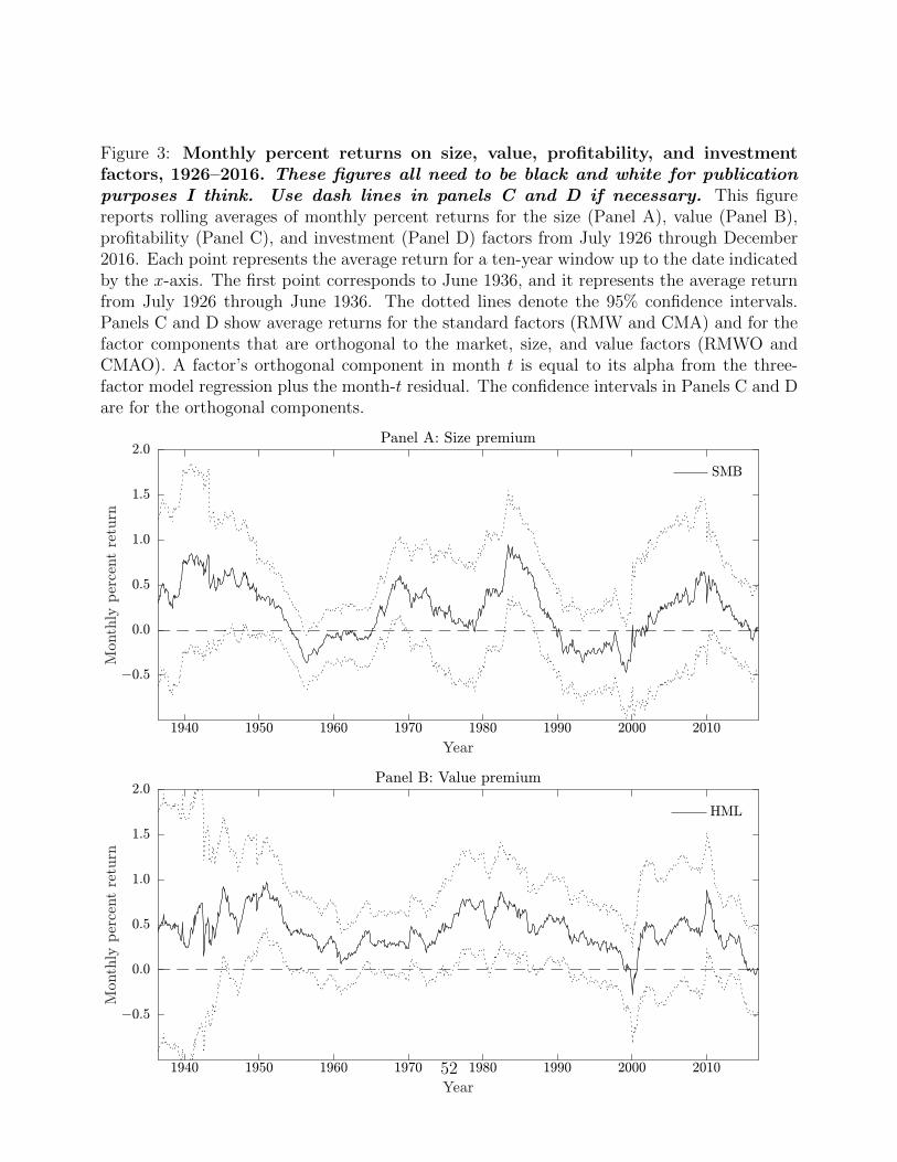
Figure 3: Monthly percent returns on size, value, profitability, and investmentfactors, 1926–2016. These figures all need to be black and white for publicationpurposes I think. Use dash lines in panels C and D if necessary. This figurereports rolling averages of monthly percent returns for the size (Panel A), value (Panel B),profitability (Panel C), and investment (Panel D) factors from July 1926 through December2016. Each point represents the average return for a ten-year window up to the date indicatedby the x-axis. The first point corresponds to June 1936, and it represents the average returnfrom July 1926 through June 1936. The dotted lines denote the 95% confidence intervals.Panels C and D show average returns for the standard factors (RMW and CMA) and for thefactor components that are orthogonal to the market, size, and value factors (RMWO andCMAO). A factor’s orthogonal component in month t is equal to its alpha from the three-factor model regression plus the month-t residual. The confidence intervals in Panels C and Dare for the orthogonal components.

52

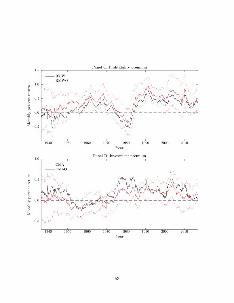
53

Figure 4: Annualized Sharpe ratios for the market portfolio and an ex-post mean-variance efficient strategy for ten-year rolling windows, 1926–2016. This figurereports Sharpe ratios for the market portfolio (thin line) and an ex-post mean-variance efficientstrategy (thick line). Each point reports the annualized Sharpe ratio for a ten-year window upto the date indicated by the x-axis. The first point corresponds to June 1936, and it representsthe Sharpe ratio from July 1926 through June 1936. The mean-variance efficient strategy iscomputed from the returns on the market, size, value, profitability, and investment factorsfrom July 1963 through December 2016. This strategy is in-sample for the post-1963 periodand out-of-sample for the pre-1963 period. The missing segment in the thick line from July1963 through May 1973 corresponds to a period during which the optimal strategy is partlyin-sample and partly out-of-sample due to the use of ten-year rolling windows.

54

Table 1: Data coverage on CRSP, Compustat, and Moody’s Industrial and Railroadmanuals, 1925–1965

This table reports the number of firms available on the Center for Research in Security PricesDatabase, Standard and Poor’s Compustat database, and Moody’s Industrial and Railroadmanuals between 1925 and 1965. The top part of the table shows the number of firms in CRSPwith and without financials (SIC codes 6000–6999) and utilities (SIC codes 4900–4999); thenumber of these firms in Compustat; and the number of these firms in either Compustat orMoody’s manuals. Except for the “full database” row, the sample excludes financials andutilities. The bottom part of the table reports, for select data items, the number of firmscovered by Compustat and the number of additional firms covered by the Moody’s manuals.

55

Year1925 1930 1935 1940 1945 1950 1955 1960 1965

Number of firms

CRSPFull database 490 748 717 784 842 998 1,058 1,113 2,164Excl. financials & utilities 458 690 665 726 778 881 926 964 1,905

Compustat 0 0 0 0 0 313 376 456 1,115Compustat + Moody’s 345 568 564 486 640 776 756 721 1,406

Number of Compustat firms by data item

Income statementRevenue 0 0 0 0 0 312 376 456 1,115Cost of goods sold 0 0 0 0 0 250 329 429 1,109Depreciation 0 0 0 0 0 310 375 455 1,105Interest 0 0 0 0 0 292 356 436 1,050Net income 0 0 0 0 0 313 376 456 1,115

Balance sheetTotal assets 0 0 0 0 0 312 375 456 1,114Total liabilities 0 0 0 0 0 277 308 394 1,043Common equity 0 0 0 0 0 0 0 2 561Accounts payable 0 0 0 0 0 0 0 2 180Receivables 0 0 0 0 0 312 375 456 1,112Inventory 0 0 0 0 0 311 374 454 1,111

Number of additional firmsfrom Moody’s manuals by data item

Income statementRevenue 186 328 389 463 598 448 374 261 291Cost of goods sold 64 187 264 416 544 399 340 247 268Depreciation 227 465 529 479 633 443 367 259 252Interest 152 347 316 254 345 280 261 197 194Net income 342 550 553 485 640 459 379 266 291

Balance sheetTotal assets 345 552 557 486 640 458 379 267 291Total liabilities 345 568 564 486 640 466 377 266 292Common equity 293 537 545 486 640 436 362 246 290Accounts payable 338 547 552 483 638 437 363 245 282Receivables 344 544 554 485 639 457 374 264 291Inventory 340 542 549 479 632 452 373 265 285

56

Table 2: Comparison to Fama-French Factors, 1963–2016

Panel A shows the average monthly percent returns and the associated t-values for thesize, value, profitability, and investment factors between July 1963 through December 2016.Panel B reports the correlations between our factors and those reported by Fama and Frenchfor the same sample period. The sample in this table includes financials (SIC codes 6000–6999)and utilities (SIC codes 4900–4999). The size (SMB) and value (HML) factors sort stocks intosix portfolios by size and book-to-market at the end of each June and hold the value-weightedportfolios from the July of year t to the June of year t+ 1. These sorts use the median NYSEbreakpoint for size and the 30th and 70th percentile NYSE breakpoints for book-to-market.SMB is the average return on the three small-stock portfolios minus the average return on thethree big-stock portfolios. HML is the average return on the two high-book-to-market port-folios minus the average return on the two low-book-to-market portfolios. The profitabilityfactor (RMW) sorts stocks into six portfolios by size and operating profitability. Operatingprofitability is revenue minus the sum of the cost of goods sold, sales, general & administra-tive expenses, and interest scaled, all scaled by the book value of equity. RMW is the averagereturn on the two high profitability (robust) portfolios minus that on the two low profitability(weak) portfolios. The investment factor (CMA) sorts stocks into six portfolios by size andgrowth in the book value of total assets. CMA is the average return on the two low investment(conservative) portfolios minus that on the two high investment (aggressive) portfolios.

Panel A: Monthly percent returnsOur factors Fama-French factors

Mean t-value Mean t-valueSize (SMB) 0.23 1.92 0.23 1.86Value (HML) 0.36 3.23 0.37 3.35Profitability (RMW) 0.25 2.94 0.24 2.74Investment (CMA) 0.25 3.49 0.31 3.91

Panel B: Correlations between our factors and Fama-French factorsFama-French factors

Our factors SMB HML RMW CMASize (SMB) 0.996Value (HML) 0.982Profitability (RMW) 0.982Investment (CMA) 0.980

57

Table 3: Monthly percent returns and alphas on size, value, profitability, andinvestment portfolios and factors, 1926–2016

Panel A reports average monthly percent returns for the size, value, profitability, and in-vestment factors, and for value-weighted portfolios that are used to construct these factors.The size and value factors are constructed by sorting stocks into portfolios by size and book-to-market; the profitability factor sorts stocks by size and profitability; and the investmentfactor by size and investment (asset growth). Profitability is revenue minus the sum of thecost of goods sold and interest expense, all divided by the book value of equity. The portfoliosare constructed using the median NYSE breakpoint for size and the 30th and 70th percentilebreakpoints for book-to-market, profitability, or asset growth. These portfolios are rebalancedannually at the end of June. Panel B reports the average number of stocks in each portfolio.Panel C reports monthly CAPM alphas for the four factors, and the three-factor model alphasfor the profitability and investment factors. The pre-1963 sample period is divided into twosegments, July 1926 through June 1938 and July 1938 through June 1963. In Panels A and Ct-values for the average monthly percent returns and alphas are reported in parentheses.

58

Panel A: Monthly percent returnsPre-1963 sample

July 1926 July 1938 July 1926 July 1963Portfolio – June 1938 – June 1963 – June 1963 – December 2016

Portfolios sorted by size and book-to-market

Small Growth 0.73 1.17 1.03 0.88Neutral 1.04 1.32 1.23 1.29Value 1.41 1.62 1.55 1.40

Big Growth 0.80 0.99 0.93 0.88Neutral 0.73 1.16 1.02 0.96Value 0.88 1.51 1.31 1.13

Size factor 0.26 0.15 0.18 0.20(0.62) (1.05) (1.11) (1.54)

Value factor 0.38 0.48 0.45 0.38(0.66) (2.87) (2.06) (3.40)

Portfolios sorted by size and profitability

Small Weak 0.88 1.32 1.18 0.96Neutral 0.78 1.38 1.19 1.24Robust 0.75 1.37 1.17 1.31

Big Weak 0.81 1.09 1.00 0.83Neutral 0.76 1.10 0.99 0.90Robust 0.68 1.23 1.05 1.03

Profitability factor −0.13 0.09 0.02 0.28(−0.31) (0.64) (0.14) (3.09)

Portfolios sorted by size and investment

Small Aggressive 0.84 1.23 1.10 0.98Neutral 1.58 1.36 1.43 1.34Conservative 1.06 1.36 1.27 1.33

Big Aggressive 0.69 1.11 0.97 0.90Neutral 1.14 1.12 1.13 0.94Conservative 0.86 1.04 0.98 1.08

Investment factor 0.19 0.03 0.09 0.26(0.79) (0.32) (0.80) (3.28)

59

Panel B: Average number of stocks in a portfolioPre-1963 sample

July 1926 July 1938 July 1926 July 1963Portfolio – June 1938 – June 1963 – June 1963 – December 2016

Portfolios sorted by size and book-to-market

Small Growth 41.5 64.3 56.9 783.4Neutral 105.7 162.3 143.9 803.9Value 127.5 170.0 156.2 861.5

Big Growth 124.5 174.3 158.1 319.3Neutral 115.6 156.4 143.2 242.9Value 36.7 68.0 57.9 99.7

Portfolios sorted by size and profitability

Small Weak 28.5 102.1 78.3 853.9Neutral 28.8 106.1 81.1 850.4Robust 25.4 80.1 62.4 736.5

Big Weak 20.7 70.2 54.2 199.3Neutral 38.0 125.5 97.1 264.7Robust 24.1 93.5 71.0 190.2

Portfolios sorted by size and investment

Small Aggressive 46.8 84.0 71.9 772.2Neutral 85.4 108.5 101.0 642.5Conservative 89.0 117.8 108.5 849.3

Big Aggressive 86.8 102.8 97.6 242.6Neutral 92.4 140.9 125.2 268.3Conservative 43.4 68.2 60.2 131.0

60

Panel C: Monthly CAPM and three-factor model alphasPre-1963 sample

July 1926 July 1938 July 1926 July 1963Factor – June 1938 – June 1963 – June 1963 – December 2016

CAPM alphas

SMB 0.15 −0.09 0.01 0.08(0.39) (0.68) (0.07) (0.62)

HML 0.12 0.23 0.11 0.44(0.27) (1.42) (0.59) (3.99)

RMW 0.02 0.19 0.20 0.30(0.06) (1.25) (1.33) (3.33)

CMA 0.17 −0.02 0.05 0.33(0.71) (−0.19) (0.49) (4.39)

Three-factor model alphas

RMW 0.06 0.30 0.25 0.35(0.18) (2.60) (1.90) (3.81)

CMA 0.12 −0.07 0.02 0.11(0.54) (−0.82) (0.16) (1.96)

61

Table 4: Defining return anomalies

This table lists the return anomalies examined in this study, the paper that first used eachvariable to predict the cross section of returns, and the sample period of returns used in thatstudy. An asterisk denotes an anomaly that is defined differently from the initial study dueto the lack of either quarterly data or some data items. The approximations are described inTable ??. The bolded anomalies—operating profitability, book-to-market, and asset growth—are the profitability, value, and investment factors studied in detail in Section 3. The anomaliesare described in the Appendix in Section A.

62

OriginalCategory No. Anomaly Original study sample

Profitability 1 Gross profitability Novy-Marx (2013) 1963–20102 Operating profitability∗ Fama and French (2015) 1963–20133 Return on assets∗ Haugen and Baker (1996) 1979–19934 Return on equity∗ Haugen and Baker (1996) 1979–19935 Profit margin Soliman (2008) 1984–20026 Change in asset turnover Soliman (2008) 1984–2002

Earnings 7 Accruals∗ Sloan (1996) 1962–1991quality 8 Net operating assets Hirshleifer, Hou, Teoh, and Zhang (2004) 1964–2002

9 Net working capital changes Soliman (2008) 1984–2002Valuation 10 Book-to-market Fama and French (1992) 1963–1990

11 Cash flow / price Lakonishok, Shleifer, and Vishny (1994) 1968–199012 Earnings / price Basu (1977) 1957–197113 Enterprise multiple∗ Loughran and Wellman (2011) 1963–200914 Sales / price Barbee, Mukherji, and Raines (1996) 1979–1991

Investment 15 Asset growth Cooper, Gulen, and Schill (2008) 1968–2003and growth 16 Growth in inventory Thomas and Zhang (2002) 1970–1997

17 Sales growth Lakonishok, Shleifer, and Vishny (1994) 1968–199018 Sustainable growth Lockwood and Prombutr (2010) 1964–200719 Adjusted CAPX growth∗ Abarbanell and Bushee (1998) 1974–199320 Growth in sales − inventory Abarbanell and Bushee (1998) 1974–199321 Investment growth rate∗ Xing (2008) 1964–200322 Abnormal capital investment∗ Titman, Wei, and Xie (2004) 1973–199623 Investment to capital∗ Xing (2008) 1964–200324 Investment-to-assets Lyandres, Sun, and Zhang (2008) 1970–2005

Financing 25 Debt issuance∗ Spiess and Affleck-Graves (1999) 1975–199426 Leverage Bhandari (1988) 1948–197927 One-year share issuance Pontiff and Woodgate (2008) 1970–200328 Five-year share issuance Daniel and Titman (2006) 1968–200329 Total external financing∗ Bradshaw, Richardson, and Sloan (2006) 1971–2000

Distress 30 O-Score Dichev (1998) 1981–199531 Z-Score∗ Dichev (1998) 1981–199532 Distress risk Campbell, Hilscher, and Szilagyi (2008) 1963–2003

Other 33 Industry concentration Hou and Robinson (2006) 1951–2001Composite 34 Piotroski’s F-score Piotroski (2000) 1976–1996anomalies 35 M/B and accruals∗ Bartov and Kim (2004) 1981–2000

36 QMJ: Profitability Asness, Frazzini, and Pedersen (2013) 1956–2012

63

Table 5: Average returns and CAPM and three-factor model alphas for 36 anoma-lies

This table reports monthly average excess returns, CAPM alphas, and three-factor modelalphas for the 36 anomalies described in Appendix A. Every anomaly is constructed as anHML-like factor by sorting stocks first into six portfolios by size and the anomaly variable atthe end of each June. The sorts use the 50 and 30/70 NYSE breakpoints except for anomaliessuch as debt issuance in which indicator variables determine the portfolio assignments. Thereturn on the anomaly factor is the average return on the two high portfolios minus that onthe two low portfolios. The high and low labels are chosen based on the original study sothat the stocks in the high portfolio earn higher returns than those in the low portfolios. Wereport the estimates for pre-sample, in-sample, and post-sample periods. In-sample period isthe period used in the original study as reported in Table 4. Pre-sample period is the periodthat predates the sample period used in the original study. Post-sample period is the samplethat has accumulated after the end of the in-sample period. The post-sample estimates arenot reported for operating profitability and QMJ: Profitability because they have less thanfive years post-sample data.

Excessreturn CAPM FF3

Anomaly Avg. t α̂ t α̂ t

Profitability

Gross profitability Pre 0.00 −0.01 0.28 1.74 0.35 2.61In 0.26 2.76 0.30 3.10 0.43 4.68Post 0.23 0.83 0.63 2.65 0.57 2.80

Operating profitability Pre −0.01 −0.06 0.17 1.11 0.22 1.66In 0.27 2.93 0.29 3.13 0.33 3.52Post . . . . . .

Return on assets Pre −0.15 −1.03 0.05 0.45 0.23 2.68In 0.18 1.18 0.21 1.40 0.53 4.44Post 0.23 1.29 0.48 3.12 0.47 3.65

Return on equity Pre −0.08 −0.63 0.04 0.31 0.22 2.37In 0.22 1.56 0.18 1.28 0.45 3.55Post 0.20 1.09 0.43 2.67 0.39 3.05

Profit margin Pre −0.11 −0.94 0.00 0.04 0.15 1.71In 0.27 1.56 0.39 2.38 0.31 2.25Post −0.14 −0.88 0.04 0.30 0.07 0.59

64

Excessreturn CAPM FF3

Anomaly Avg. t α̂ t α̂ tChange in asset turnover Pre 0.07 0.83 0.09 1.14 0.11 1.43

In 0.49 4.49 0.52 4.72 0.55 5.03Post −0.05 −0.52 −0.06 −0.55 −0.07 −0.67

Earnings quality

Accruals Pre 0.10 1.02 0.10 1.01 0.08 0.81In 0.25 2.82 0.31 3.75 0.22 2.83Post 0.18 1.87 0.14 1.52 0.16 1.67

Net operating assets Pre 0.11 1.37 0.09 1.07 0.10 1.29In 0.30 3.80 0.29 3.71 0.38 5.03Post 0.11 0.80 0.08 0.61 0.07 0.59

Net working capital changes Pre 0.26 3.98 0.30 4.64 0.27 4.21In 0.21 2.06 0.23 2.27 0.26 2.48Post 0.01 0.12 −0.02 −0.18 −0.01 −0.13

Valuation

Book-to-market Pre 0.44 2.05 0.10 0.58 −0.02 −0.64In 0.46 3.22 0.51 3.73 0.01 0.15Post 0.31 1.72 0.36 2.00 0.00 0.05

Cash flow / price Pre 0.17 1.51 0.15 1.26 0.13 1.13In 0.69 4.38 0.74 4.93 0.23 3.43Post 0.23 1.12 0.40 2.01 0.10 0.88

Earnings / price Pre 0.12 0.62 0.30 1.57 0.35 2.05In 0.43 2.85 0.53 3.70 0.30 3.11Post 0.37 2.62 0.53 3.94 0.20 2.13

Enterprise multiple Pre 0.17 1.08 0.24 1.56 0.22 1.44In 0.36 3.06 0.46 4.21 0.12 1.70Post −0.14 −0.80 −0.21 −1.11 −0.20 −1.36

Sales / price Pre 0.25 2.35 0.17 1.65 0.06 0.69In 0.34 1.87 0.39 2.15 0.07 0.55Post 0.39 1.94 0.49 2.39 0.10 0.87

65

Excessreturn CAPM FF3

Anomaly Avg. t α̂ t α̂ t

Investment and growth

Asset growth Pre 0.06 0.64 0.03 0.33 −0.02 −0.25In 0.40 3.75 0.48 4.97 0.19 2.66Post 0.05 0.45 0.01 0.06 −0.01 −0.05

Growth in inventory Pre 0.20 2.70 0.20 2.61 0.18 2.49In 0.29 3.24 0.36 4.26 0.20 2.61Post 0.18 1.69 0.17 1.63 0.15 1.42

Sales growth Pre 0.11 0.68 0.04 0.28 −0.01 −0.04In 0.24 2.06 0.28 2.55 0.02 0.27Post −0.10 −0.81 −0.01 −0.04 −0.18 −2.01

Sustainable growth Pre 0.05 0.38 −0.04 −0.35 −0.10 −1.02In 0.15 1.57 0.24 2.60 −0.05 −0.64Post 0.13 0.89 0.11 0.79 0.17 1.37

Adjusted CAPX growth Pre 0.14 1.78 0.06 0.86 0.03 0.43In 0.21 2.70 0.24 3.12 0.13 1.71Post 0.03 0.27 0.09 0.92 0.03 0.30

Growth in sales - inventory Pre 0.09 0.76 0.15 1.31 0.22 2.13In 0.40 4.93 0.39 4.76 0.42 4.97Post 0.10 1.04 0.10 1.09 0.14 1.61

Investment growth rate Pre 0.07 0.76 0.09 1.05 0.09 1.01In 0.26 4.29 0.30 5.13 0.21 3.67Post −0.09 −0.94 −0.06 −0.66 −0.06 −0.70

Abnormal capital investment Pre 0.10 0.94 0.12 1.13 0.15 1.44In 0.21 3.30 0.20 3.22 0.16 2.46Post −0.03 −0.33 −0.02 −0.21 −0.02 −0.24

Investment to capital Pre 0.20 2.24 0.19 2.13 0.18 2.01In 0.18 1.49 0.31 2.96 0.03 0.37Post 0.05 0.36 0.06 0.43 0.05 0.50

Investment-to-assets Pre 0.26 3.24 0.25 3.16 0.23 3.00In 0.27 3.24 0.34 4.26 0.19 2.44Post 0.23 1.84 0.19 1.51 0.20 1.67

66

Excessreturn CAPM FF3

Anomaly Avg. t α̂ t α̂ t

Financing

Debt issuance Pre 0.05 0.82 0.10 1.76 0.11 2.07In 0.18 3.99 0.19 4.01 0.19 4.06Post 0.11 1.50 0.08 1.05 0.14 2.28

Leverage Pre 0.08 0.48 −0.08 −0.63 −0.11 −0.95In 0.21 2.65 0.19 2.33 0.01 0.12Post 0.18 1.28 0.19 1.36 −0.18 −2.22

One-year share issuance Pre 0.26 2.47 0.34 3.25 0.37 3.70In 0.27 2.71 0.38 4.21 0.20 2.80Post 0.04 0.31 0.13 1.29 0.13 1.44

Five-year share issuance Pre 0.09 1.20 0.18 2.43 0.20 2.77In 0.24 2.39 0.34 3.67 0.17 2.42Post 0.12 1.24 0.20 2.24 0.20 2.40

Total external financing Pre −0.13 −1.16 0.07 0.81 0.12 1.58In 0.34 2.61 0.52 4.82 0.33 4.21Post 0.19 1.06 0.34 2.31 0.30 2.66

Distress

O-Score Pre −0.05 −0.33 0.21 2.01 0.32 3.84In 0.27 1.97 0.35 2.71 0.51 4.41Post −0.08 −0.68 0.04 0.33 0.09 0.83

Z-Score Pre −0.23 −1.53 0.02 0.18 0.19 2.28In 0.14 0.82 0.07 0.40 0.59 4.74Post −0.09 −0.53 −0.06 −0.36 0.14 1.28

Distress risk Pre 0.08 0.34 0.40 1.91 0.47 2.75In 0.39 2.34 0.60 4.26 0.56 4.69Post 0.18 0.79 0.47 2.76 0.44 2.92

Other

Industry concentration Pre 0.04 0.27 −0.02 −0.10 −0.05 −0.32In 0.09 1.06 0.01 0.17 0.18 2.18Post −0.13 −0.77 −0.21 −1.33 −0.17 −1.29

67

Excessreturn CAPM FF3

Anomaly Avg. t α̂ t α̂ t

Composite anomalies

Piotroski’s F-score Pre 0.07 0.67 0.14 1.41 0.19 1.92In 0.47 5.20 0.53 5.92 0.61 7.08Post 0.11 0.66 0.27 1.85 0.21 1.69

M/B and accruals Pre 0.56 2.54 0.45 2.08 0.20 1.18In 0.62 2.34 0.86 3.33 0.25 1.25Post 0.36 1.00 0.30 0.86 −0.20 −0.74

QMJ: Profitability Pre 0.04 0.17 0.36 1.72 0.42 2.29In 0.22 2.70 0.31 4.06 0.47 7.09Post . . . . . .

68

Table 6: Measuring changes in average returns, alphas, and information ratiosbetween pre-, in-, and post-sample periods

This table compares the performance of the average anomaly between the sample periodused in the original study (in-sample) and the periods that predate or follow the originalsample period (pre- and post-sample). Panel A uses data starting in July 1926. Panel B usesdata back to July 1938. We estimate average monthly returns, variance ratios, annualizedvolatilities, CAPM alphas, and three-factor model alphas for the 36 anomalies listed in theAppendix. The list of anomalies excludes book-to-market, and the post-discovery anomaly listadditionally excludes the two anomalies, “Operating profitability” and “QMJ: Profitability,”with less than five years of post-discovery out-of-sample data. Variance ratio is the varianceof factor returns divided by the return variance of a randomized factor. The randomizedfactor takes the same stocks as the actual factor and randomly sorts them into low, neutral,and high portfolios. Annualized information ratios from the CAPM and three-factor modelsequal

√12× α̂/σ̂ε, where σ̂ε is the volatility of the regression residuals. We report t-values in

parentheses. We compute the standard errors by block bootstrapping the data by calendarmonth 10,000 times.

69

Panel A: Full pre-1963 sampleDifferences

Pre- In- Post- Pre Post PostMeasure sample sample sample − In − In − Pre

Average returns

Average return 0.07 0.29 0.09 −0.21 −0.20 0.02(1.92) (6.91) (1.84) (−3.81) (−3.56) (0.25)

Sharpe ratio 0.13 0.54 0.14 −0.41 −0.41 0.00(2.80) (7.47) (1.66) (−4.91) (−4.04) (0.04)

Excess volatility 3.66 3.57 3.84 0.09 0.30 0.17(4.79) (15.36) (12.08) (0.16) (1.69) (0.28)

CAPM

Alpha 0.14 0.34 0.17 −0.20 −0.18 0.03(4.42) (9.54) (3.46) (−4.33) (−3.39) (0.49)

Information ratio 0.20 0.65 0.26 −0.45 −0.40 0.06(4.53) (9.46) (2.91) (−5.62) (−3.84) (0.59)

Three-factor model

Alpha 0.16 0.27 0.12 −0.10 −0.14 −0.04(5.94) (10.14) (3.16) (−2.70) (−3.39) (−0.94)

Information ratio 0.25 0.59 0.25 −0.34 −0.35 −0.01(5.62) (9.85) (2.82) (−4.60) (−3.46) (−0.07)

70

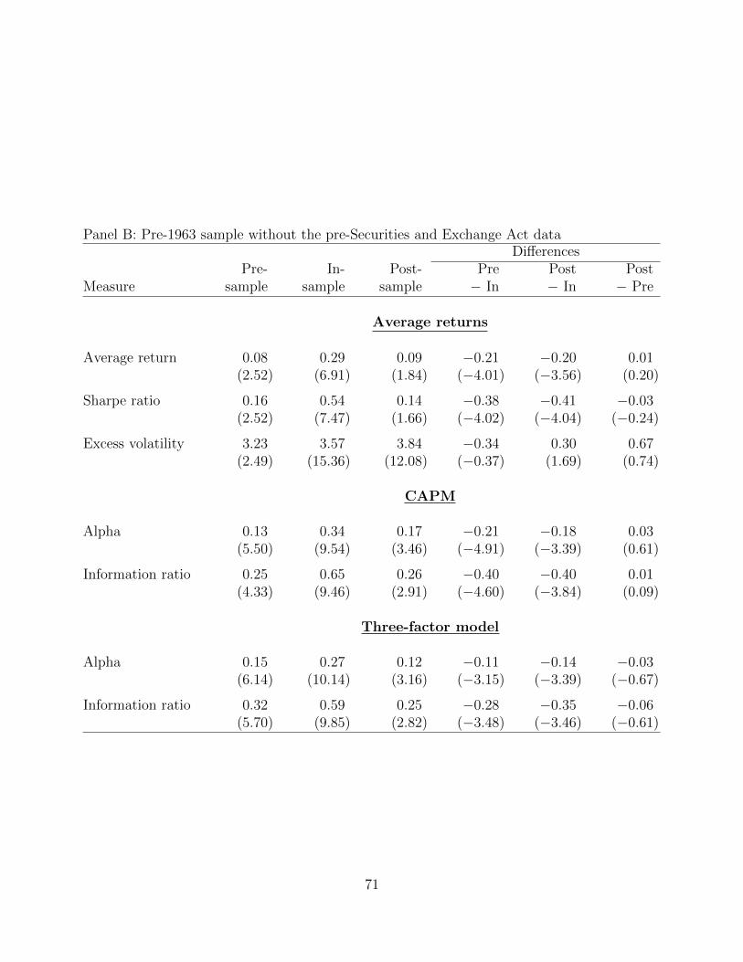
Panel B: Pre-1963 sample without the pre-Securities and Exchange Act dataDifferences

Pre- In- Post- Pre Post PostMeasure sample sample sample − In − In − Pre

Average returns

Average return 0.08 0.29 0.09 −0.21 −0.20 0.01(2.52) (6.91) (1.84) (−4.01) (−3.56) (0.20)

Sharpe ratio 0.16 0.54 0.14 −0.38 −0.41 −0.03(2.52) (7.47) (1.66) (−4.02) (−4.04) (−0.24)

Excess volatility 3.23 3.57 3.84 −0.34 0.30 0.67(2.49) (15.36) (12.08) (−0.37) (1.69) (0.74)

CAPM

Alpha 0.13 0.34 0.17 −0.21 −0.18 0.03(5.50) (9.54) (3.46) (−4.91) (−3.39) (0.61)

Information ratio 0.25 0.65 0.26 −0.40 −0.40 0.01(4.33) (9.46) (2.91) (−4.60) (−3.84) (0.09)

Three-factor model

Alpha 0.15 0.27 0.12 −0.11 −0.14 −0.03(6.14) (10.14) (3.16) (−3.15) (−3.39) (−0.67)

Information ratio 0.32 0.59 0.25 −0.28 −0.35 −0.06(5.70) (9.85) (2.82) (−3.48) (−3.46) (−0.61)

71

Table 7: Estimating the effect of the start date on anomaly excess returns andCAPM and three-factor model alphas

This table reports estimates from panel regressions that estimate the effect of the start dateon anomaly excess returns and CAPM and three-factor model alphas. The dependent variableis an anomaly’s excess return, the constant plus residual from the CAPM regression, or theconstant plus residual from the three-factor model regression. The beginning of the sampleperiod is indicated in the first column. For each anomaly, we include data up to the end ofthe in-sample period. The regressions only include anomalies whose in-sample periods beginafter the first column’s start date. The regression is

anomalyit = β0 + β1Pre-sampleit + µi + εit,

where (i, t) indexes (anomaly, month), Pre-sampleit is an indicator equal to one if the anomaly-month observation falls in the time period before the start-date of the anomaly’s in-samplestart date, µi is an anomaly fixed effect, and εit is a error term. We exclude from the samplethe book-to-market anomaly and the two anomalies that are annual versions of originallyquarterly anomalies (return on assets and return on equity). Standard errors are clustered bycalendar month.

72

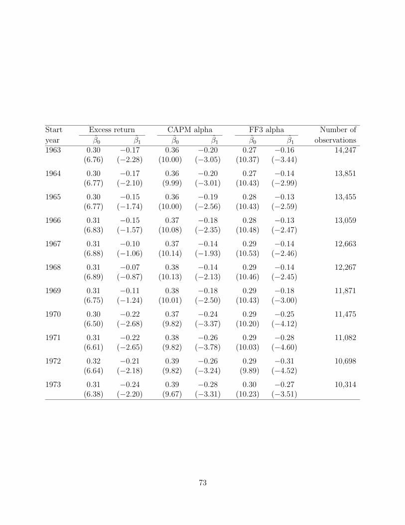
Start Excess return CAPM alpha FF3 alpha Number of

year β̂0 β̂1 β̂0 β̂1 β̂0 β̂1 observations1963 0.30 −0.17 0.36 −0.20 0.27 −0.16 14,247

(6.76) (−2.28) (10.00) (−3.05) (10.37) (−3.44)

1964 0.30 −0.17 0.36 −0.20 0.27 −0.14 13,851(6.77) (−2.10) (9.99) (−3.01) (10.43) (−2.99)

1965 0.30 −0.15 0.36 −0.19 0.28 −0.13 13,455(6.77) (−1.74) (10.00) (−2.56) (10.43) (−2.59)

1966 0.31 −0.15 0.37 −0.18 0.28 −0.13 13,059(6.83) (−1.57) (10.08) (−2.35) (10.48) (−2.47)

1967 0.31 −0.10 0.37 −0.14 0.29 −0.14 12,663(6.88) (−1.06) (10.14) (−1.93) (10.53) (−2.46)

1968 0.31 −0.07 0.38 −0.14 0.29 −0.14 12,267(6.89) (−0.87) (10.13) (−2.13) (10.46) (−2.45)

1969 0.31 −0.11 0.38 −0.18 0.29 −0.18 11,871(6.75) (−1.24) (10.01) (−2.50) (10.43) (−3.00)

1970 0.30 −0.22 0.37 −0.24 0.29 −0.25 11,475(6.50) (−2.68) (9.82) (−3.37) (10.20) (−4.12)

1971 0.31 −0.22 0.38 −0.26 0.29 −0.28 11,082(6.61) (−2.65) (9.82) (−3.78) (10.03) (−4.60)

1972 0.32 −0.21 0.39 −0.26 0.29 −0.31 10,698(6.64) (−2.18) (9.82) (−3.24) (9.89) (−4.52)

1973 0.31 −0.24 0.39 −0.28 0.30 −0.27 10,314(6.38) (−2.20) (9.67) (−3.31) (10.23) (−3.51)

73

Table 8: Out-of-sample valuation versus statistical adjustments

This table reports three sets of anomalies. The first set in the leftmost column containsanomalies identified as having statistically significant Fama-French three factor alphas in thepre-sample period. The second set in the middle column contains anomalies identified ashaving statistically significant Fama-French three factor alphas based on a t-statistic thresholdof 3.00, as suggested by Harvey, Liu, and Zhu (2015). The third set in the rightmost columncontains the intersection of the first two sets.

Significant In-sampleAnomaly in pre-sample t-value > 3 Union

Gross profitability R R R

Operating profitability R

Return on assets R R R

Return on equity R R R

Change in asset turnover R

Net operating assets R

Net working capital changes R

Cash flow / price R

Earnings / price R R R

Growth in inventory R

Growth in sales − inventory R R R

Investment growth rate R

Investment to capital R

Investment-to-assets R

Debt issuance R R R

One-year share issuance R

Five-year share issuance R

Total external financing R

O-Score R R R

Z-Score R R R

Distress risk R R R

Piotroski’s F-score R

QMJ: Profitability R R R

Count 16 17 10

74

Table 9: Changes in the correlation structure of returns

This table reports estimates from panel regressions of monthly anomaly returns on the averagereturns on all other anomalies that are either in-sample or out-of-sample. In the first regres-sion, posti,t takes the value of one if anomaly i is in the post-sample period in month t and zerootherwise; in-sample index−i,t is the average return on all anomalies except anomaly i that arein-sample in month t; and post-sample index−i,t is the average return on all anomalies exceptanomaly i that are in the post-sample period in month t. In the second regression, prei,ttakes the value of one if anomaly i is in the pre-sample period in month t and zero otherwise;in-sample index−i,t is the average return on all anomalies except anomaly i that are in-samplein month t; and pre-sample index−i,t is the average return on all anomalies except anomaly ithat are in the pre-sample period in month t.

75

Regressor Coefficient t-value

Regression 1: In-sample versus post-sample anomalies

Intercept 0.05 4.50Main effects

In-sample index−i,t 0.71 29.59Post-sample index−i,t 0.10 7.69Posti,t −0.06 −2.27

InteractionsPosti,t × In-sample index−i,t −0.50 −12.51Posti,t × Post-sample index−i,t 0.44 10.40

Adjusted R2 17.6%N 14,639

Regression 2: In-sample versus pre-sample anomalies

Intercept 0.07 4.24Main effects

In-sample index−i,t 0.74 29.42Pre-sample index−i,t 0.07 3.40Prei,t −0.05 −2.18

InteractionsPrei,t × In-sample index−i,t −0.69 −22.80Prei,t × Pre-sample index−i,t 0.49 14.37

Adjusted R2 9.8%N 13,254

76