Credit Ratings and The Cross-Section of Stock Returns

Credit Ratings and The Cross-Section of StockReturns

Doron Avramov∗

Department of Finance

Robert H. Smith School of Business

University of Maryland

[email protected]

Tarun Chordia


Goizueta Business School

Emory University

Tarun [email protected]

Gergana Jostova


School of Business

George Washington University

[email protected]

Alexander Philipov


Kogod School of Business

American University

[email protected]

Preliminary

Credit Ratings and The Cross-Section of StockReturns

Abstract

Firms with low credit risk realize higher returns than firms with high credit risk.

This credit risk effect in the cross-section of stock returns is a puzzle because in-

vestors appear to pay a premium for bearing credit risk. This paper shows that the

negative relation between credit risk and returns is statistically and economically

significant only during periods of credit rating downgrades. During such periods,

low quality firms experience substantial deterioration in their operating and finan-

cial performance, and are sold by institutional investors leading to considerable

price drops. The deteriorating fundamental performance is unanticipated by the

market as evidenced by the large negative earnings surprises and analyst forecast

revisions. In contrast, average returns do not differ across credit risk groups in

periods of stable or improving credit conditions, which account for about 90% of

the sample observations.

Introduction

It is a fundamental principle of financial economics that higher risk assets should com-

mand higher expected returns. This risk-return tradeoff underlies the conceptual frame-

work of asset pricing and investment decisions in efficient markets. Empirically, however,

Dichev (1998) and Campbell, Hilscher, and Szilagyi (2005), among others, demonstrate

that credit risk is negatively related to the cross-section of stock returns. This evidence

is anomalous because investors appear to pay a premium for bearing credit risk.

This paper examines the credit risk effect in the cross-section of stock returns during

credit cycles. Our analysis is based on a comprehensive sample of 3,578 NYSE, AMEX,

and NASDAQ firms rated by S&P over the July 1985-December 2003 period.1 We

first show that the return differential between the highest and lowest rated stock decile

is 1.16% (7.60%) over a one month (year) period after the portfolio formation date,

and we confirm the negative relation between credit ratings and returns using Fama

and MacBeth (1973) cross-sectional regressions of monthly individual stock returns on

credit rating. Moreover, we use the CAPM of Sharpe (1964) and Lintner (1965) and the

Fama and French (1993) three-factor model, as well as the characteristic based model

of Daniel, Grinblatt, Titman, and Wermers (1997) to demonstrate that the negative

relation between credit risk and returns is robust to adjustments for risk as well as for

firm characteristics.

The negative relation between credit risk and average returns crucially depends on

credit cycles. In particular, the relationship prevails due to returns over downgrade

periods extending from six months before to six months after credit rating downgrades.

Also, it is the returns on low rated stocks that drive the negative relation between credit

risk and returns. In contrast, the credit risk effect is statistically and economically

insignificant during periods of stable or improving credit conditions, which capture about

90% of the overall sample observations. In particular, from an economic perspective,

trading strategies that sell low credit risk and buy high credit risk stocks during non-

downgrade periods provide small and insignificant payoffs. Moreover, credit rating is

statistically and economically insignificant in monthly cross sectional regressions during

non-downgrade periods.

1We use the S&P Long-Term Domestic Issuer Credit Rating. Data on this variable is available onCompustat on a quarterly basis starting from the second quarter of 1985.

1

Indeed, previous work (e.g., Hand, Holthausen, and Leftwich (1992) and Dichev

and Piotroski (2001)) documents considerable abnormal price declines following rating

downgrades. Relative to this body of work, however, we uncover substantial cross section

differences in stock price responses to rating downgrades. The considerable stock price

drop following rating downgrades is apparent among low quality stocks, whereas high

quality firms often realize positive returns around rating downgrades. It is the differential

response of high and low credit risk stocks to rating downgrades that gives rise to the

negative relation between credit risk and stock returns.

The significant credit risk effect during periods of worsening credit conditions re-

veals yet another puzzle. In particular, we show that rating downgrades are larger in

magnitude and frequency among low rated than among high rated firms. Hence, one

would expect lower rated stocks to command even higher expected returns than higher

rated stocks during periods of worsening credit conditions. However, high credit risk

stocks continue to realize far lower returns than low credit risk stocks for upto two years

following a downgrade.

To understand the stock price responses to credit rating downgrades among the

credit risk groups, we analyze the operating and financial performance of firms around

downgrades. Specifically, we examine industry-adjusted accounting ratios including sales

growth, profit margin, net cash flow, interest coverage, and asset turnover. The evidence

suggests that the fundamental performance of the low rated stocks is substantially worse

than that of the high rated stocks both before and after a rating downgrade. The dete-

riorating fundamental performance or low rated stocks around downgrades is consistent

with the severe decline in their prices.

More importantly, the deteriorating performance of high credit risk stocks both be-

fore and after rating downgrades is not anticipated by the market as evidenced by analyst

forecast revisions and earnings surprises. Analyst forecast revisions and earnings sur-

prises around downgrades are negative and much larger in absolute values for low rated

stocks for up to a year after the downgrade. Moreover, institutions reduce their hold-

ings of the low rated stocks around rating downgrades possibly due to their fiduciary

responsibilities. One reason for why analysts and institutions are surprised by the poor

fundamental performance of the low rated stocks may be due to the fact that financial

distress itself may prompt suppliers, customers, creditors and employees to abandon

these firms in larger than expected numbers around downgrades. Given the significantly

2

higher illiquidity of low rated stocks, the institutional selling activity, following the neg-

ative surprises among high credit risk stocks, may be the cause of the substantial stock

price drop, and ultimately the negative relation between credit risk and returns.

The rest of the paper is organized as follows. The next section discusses the data.

Section 2 presents the results and section 3 concludes.

1 Data

We extract monthly returns on all NYSE, AMEX, and NASDAQ stocks listed in the

CRSP database, subject to the requirement that, at the beginning of each month, the

stock price be at least $1. While this is done to ensure that the empirical findings

are not driven by low priced and extremely illiquid stocks, we find that our results

are robust to the inclusion of stocks below $1. Throughout the paper, we use delisted

returns whenever appropriate. This is important because a number of stocks delist due

to financial distress.

The filtering procedure delivers a universe of 13,018 stocks. From this universe,

we choose those stocks that are rated by Standard & Poor’s, leaving us with 3,578

rated stocks over the July 1985 through December 2003 period. The total number of

month-return observations in our sample is 434,746. The beginning of our sample is

determined by the first time firm ratings by Standard & Poor’s become available on the

COMPUSTAT tapes. This investment universe of 3,578 rated firms forms the basis for

our analysis of the relation between firm credit rating and average returns.

The S&P issuer rating used here is an essential component of our analysis. Note that

Standard & Poor’s assigns this rating to a firm, not a bond. As defined by S&P, prior

to 1998, this issuer rating is based on the firm’s senior publicly traded debt. After 1998,

this rating is based on the overall quality of the firm’s outstanding debt, either public or

private. Before 1998, the issuer rating represents a select subsample of company bonds.

After 1998, it represents all company debt. This rating is available from COMPUSTAT

on a quarterly basis starting in 1985.

For the empirical analysis that follows, we transform the S&P ratings into con-

ventional numerical scores. In particular, AAA takes on the value 1 and D takes on

3

the value 22.2 Thus, a higher numerical score corresponds to a lower credit rating or

higher credit risk. Numerical ratings at or below 10 (BBB− or better) are considered

investment-grade, and ratings of 11 or higher (BB+ or worse) are labeled high-yield or

non-investment grade. The equally weighted average rating of the 3,578 firms in our

sample is 8.83 (approximately BBB, the investment-grade threshold) and the median is

9 (BBB).

2 Results

To confirm the credit risk return puzzle, we present in Panel A of Table 1 the time-series

average monthly return of decile portfolios sorted, every month, based on the firm’s

credit rating. Portfolio returns are the equally weighted averages of individual stock

returns in the month subsequent to portfolio formation. The mean monthly return for

the highest (lowest) credit rating portfolio C1 (C10) is 1.34% (0.17%) per month. The

difference in mean returns between the highest and the lowest rating portfolio, C1−C10,

is a statistically and economically significant 1.16% per month. This return differential

persists over several months. Specifically, the C1−C10 cumulative return over the six (12)

[24] months subsequent to portfolio formation is 4.02% (7.60%) [13.14%]. The C1 −C10

returns are even higher in non-January months (1.71% per month) and negative in

January (-5.01% per month). The average return is 1.08% per month during expansions

and 2.24% (albeit statistically insignificant) during recessions.3

The overall evidence is consistent with prior work and it represents an anomalous

pattern in the cross-section of returns because investors are expected to demand higher

risk premia and thus higher expected returns for stocks with higher credit risk. However,

the empirical evidence is exactly the opposite. Even if credit risk does not measure

systematic risk and can be diversified away, the results are anomalous because with

diversifiable risk the return differential between high and low rated stocks should be

zero. Instead the monthly return differential is 1.16%.

Before we continue with the analysis, it should be noted that a large fraction of the

2The entire spectrum of ratings is as follows. AAA=1, AA+=2, AA=3, AA−=4, A+=5,A=6, A−=7, BBB+=8, BBB=9, BBB−=10, BB+=11, BB=12, BB−=13, B+=14, B=15, B−=16,CCC+=17, CCC=18, CCC−=19, CC=20, C=21, D=22.

3The business cycle expansions and recessions are as defined by the NBER. Seewww.nber.org/cycles.html.

4

C1 −C10 payoff is generated by the lowest rated stock portfolio C10. For instance, while

the overall C1 − C10 return is 1.16% per month, the return to the portfolio C1 − C9 is

less than half that amount at 0.47% per month. Moreover, the cumulative six (12) [24]

month return for the C1−C9 portfolio is only 2.41% (5.23%) [10.18%] compared to 4.02%

(7.60%) [13.14%] for the C1 − C10 portfolio. Similarly, the return in the non-January

months for C1 − C9 is only 0.77% per month as compared to 1.71% for the C1 − C10

portfolio. Of course, the payoff for the C1 − C9 portfolio, even though smaller, is still

anomalous.

Next, we explore whether the return differential between the high and low rated

stocks can be explained by the size, value, and momentum effects in the cross-section

of stock returns. Following Daniel, Grinblatt, Titman, and Wermers (1997), we adjust

individual stock returns for size, book-to-market ratio, and past returns. In particular,

we form 5× 5× 5 size, book-to-market, and past-twelve-month return sorted portfolios.

We subtract the monthly return of the portfolio to which a stock belongs from the

individual monthly stock return to obtain the stock’s characteristic-adjusted return.

The mean characteristic-adjusted returns are summarized in Panel B of Table 1.

Notice that the C1 − C10 portfolio still realizes a payoff which is significant at 0.94%

per month, only slightly lower than the 1.16% raw return. The characteristic-adjusted

payoff earned by the C1 − C9 portfolio is 0.51% per month, slightly higher than the

0.47% unadjusted payoff. The monthly C1 −C10 characteristic-adjusted return is signif-

icant at 0.87% during expansions and 1.18% in non-January months. The cumulative

characteristic-adjusted return generated by the C1 − C10 portfolio over six (12) [24]

months subsequent to the portfolio formation date is 3.68% (6.02%) [9.16%]. Overall,

the C1−C10 characteristic-adjusted returns are significantly positive. That is, adjusting

for the traditional anomalies does not resolve the puzzle that higher credit risk stocks

earn lower returns, suggesting that the credit risk effect in the cross-section of return is

unrelated to the size, book-to-market, and momentum effects.

Table 2 documents the average characteristics of the stocks in the different decile

portfolios sorted by credit rating. The average characteristic is first calculated each

month for each stock. The portfolio characteristic is the equally weighted average each

month. Finally, these monthly averages are averaged over time to obtain the portfolio

characteristics that are reported. Firm size, as measured by market capitalization, de-

creases monotonically with credit risk. The highest rated stocks have an average market

5

capitalization of $4.91 billion while the lowest rated stocks have an average capitaliza-

tion of $0.15 billion. Average stock price also decreases monotonically from $46 for

the highest rated stocks to $7 for the lowest rated stocks. The book-to-market ratio

increases with credit risk probably due to the low market values of the low rated stocks.

Analyst following decreases monotonically with credit risk from about 19 for the high

rated stocks to 4 for the low rated stocks. Institutions hold far fewer shares of the low

rated stocks. Institutional shareholding amounts to over 50% for the high rated stocks

and about 25% for the low rated stocks. Analyst revisions and earnings surprises are

far lower and negative for the low rated stocks as compared to the high rated stocks.

Surprisingly, turnover is higher for the low rated stocks, especially amongst firms listed

on Nasdaq.

Low rated stocks are more illiquid than the high rated stocks. Illiquidity is computed

as in Amihud (2002). Amihud (2002)’s illiquidity measure is the average daily price

impact of order flow and is computed as the absolute price change per dollar of daily

trading volume:

ILLIQit =1

Dit

Dit∑

t=1

|Ritd|DV OLitd

∗ 106, (1)

where Ritd is the daily return, DV OLitd is the dollar trading volume of stock i on day

d in month t, and Dit is the number of days in month t for which data is available for

stock i. We compute Amihud (2002)’s illiquidity measure at the monthly frequency. We

require at least ten days with trades each month.4

We next confirm that the credit risk effect is significant in explaining cross-sectional

differences in individual stock returns, by running cross-sectional regressions of stock re-

turns on credit rating, while controlling for additional firm characteristics. Each month,

we run the following cross-sectional Fama and MacBeth (1973) regressions:

Rjt = at + bt RATINGjt−1 +

M∑

m=1

cmt Cmjt−2 + ejt, (2)

where RATING represents the numerical score attached to firm rating. Recall that

a higher numerical rating score corresponds to higher credit risk. Cmjt is the value of

characteristic m for security j at time t, and M is the total number of characteristics.

4Hasbrouck (2005) compares effective and price-impact measures estimated from daily data to thosefrom high-frequency data and finds that Amihud (2002)’s measure is the most highly correlated withtrade-based measures.

6

The firm characteristics included are (i) Size: Firm size measured as the market value

of equity, (ii) BM: Ratio of book value of equity to market value of equity calculated

following the procedure in Fama and French (1992), (iii) Turnover: Measured as the ratio

of monthly share trading volume to the number of shares outstanding, (iv) R(t−7:t−2):

Cumulative return over the last six months. All the characteristics are lagged by two

months relative to the month in which the dependent variable is measured. Turnover is

measured separately for NYSE-AMEX and Nasdaq stocks. Panel A of Table 3 presents

the results. We report the time-series averages of the coefficients bt and ct. The standard

errors of these estimators are obtained from the time-series of the monthly estimates.

Panel A in Table 3 shows that the coefficient of the lagged credit rating variable is

-0.07 (t− stat = −2.01). In other words, a one point higher numerical credit score (one

point worse credit rating) produces 7 basis points lower returns per month on average.

The second regression in Panel A excludes the credit rating and retains only the lagged

characteristics as independent variables. Of the characteristics, only the past six month

return has a significant impact on the cross-section of returns. The third regression

contains both credit rating and firm characteristics. It is evident that the negative

credit risk–return relation is significant and of the same magnitude whether or not firm

characteristics are included as control variables.

Indeed, results based both on raw and characteristic-adjusted portfolio returns and

on individual stock returns do conclusively suggest that higher rated stocks realize higher

returns than lower rated stocks. However, credit risk is just one measure of the firm’s

overall risk. While credit risk measures the risk that creditors may not get repaid,

it should be related to a firm’s overall risk. Barring the agency problems between

bondholders and shareholders the risk faced by both should relate to the underlying

cash flow risk of the firm. This is what we check next. We now ensure that risk as

measured using the standard asset pricing models does not capture the negative relation

between credit risk and returns. We risk-adjust raw returns using the Capital Asset

Pricing Model (CAPM) of Sharpe (1964) and Lintner (1965) as well as the Fama and

French (1993) three factor model.

Our risk adjustment is based on cross-sectional asset-pricing tests with individual

stocks. Following Brennan, Chordia, and Subrahmanyam (1998), we first run time-series

regressions of individual stock returns on the risk factors prescribed by the CAPM and

Fama-French model. We then run cross sectional regressions of risk-adjusted returns

7

on credit rating, as well the size, book-to-market, turnover, and past returns charac-

teristics. Under the null of exact pricing, credit rating as well as equity characteristics

should be statistically insignificant in the cross-sectional regressions. The cross sectional

regressions take the form

Rjt − Rft −K∑

k=1

βjkFkt = at + bt RATINGjt−1 +M∑

m=1

cmt Cmjt−2 + ejt, (3)

where βjk is the beta estimated by a first-pass time-series regression of the firm’s stock

return on the asset pricing factors over the entire sample period with non-missing returns

data.5

Panel B of Table 3 risk adjusts raw returns using the CAPM. The first regression

specification, which does not include any of the characteristic except for credit rating,

shows that the coefficient of RATING is a statistically significant -0.09, suggesting that a

one point higher numerical credit score leads to 9 basis points lower risk-adjusted returns.

As with raw returns, the credit rating coefficient remains unchanged controlling for size,

book-to-market, past returns, and turnover.

In Panel C of Table 3, the individual stock returns are risk-adjusted using the Fama

and French (1993) factors.6 The RATING coefficient is -0.08 as the equity charac-

teristics are absent from the monthly cross-sectional regressions and -0.09 when those

characteristics serve as control variables.

Note that in Table 1 the difference in rating between the highest rating decile port-

folio, AA, and the lowest rating decile portfolio, B-, is 14 rating points. This difference

should result in a return differential of 1.12% (14 × 0.08), which is comparable to the

1.16% reported in Panel A of Table 1.

In sum, the puzzling evidence that lower rated, high credit risk stocks earn lower

returns than higher rated, low credit risk stocks is robust to adjusting raw returns by

common risk factors as well as equity characteristics.

5While this entails the use of future data in calculating the factor loadings, Fama and French (1992)show that this forward looking does not impact any of the results (see also Avramov and Chordia(2006)).

6We have also checked, (results available upon request) that the results are the same when adjustingwith the Fama-French (1993) factors augmented with the momentum factor.

8

2.1 The impact of downgrades

Thus far we have documented that the credit rating level is negatively related to the

cross section of returns. Credit rating downgrade events enable one to delve deeper into

the economics of the credit-risk-return relation. Our focus on downgrades is motivated

by previous work, which demonstrates an asymmetric response of future returns to credit

rating changes. In particular, both Hand, Holthausen, and Leftwich (1992) and Dichev

and Piotroski (2001) document considerable abnormal price declines following rating

downgrades but no price advances following upgrades. We extend this analysis by looking

at the differential response of high and low credit risk stocks to rating downgrades. Since

we have data on credit rating from the quarterly COMPUSTAT tapes, we only know

the quarter in which the downgrade occurred and we do not know the exact month of

the downgrade. In the following analysis, we assume that the downgrade occurs in the

second month of quarter, i.e., in the middle of the quarter. Qualitatively, the results do

not change when we assume that the downgrade occurred in the first or the third month

of the quarter.

Table 4 provides a comprehensive summary of credit rating downgrades both by

credit risk (Panel A) and by frequency of downgrades (Panel B). The first two rows

in Panel A present the number and size of credit rating downgrades as well as returns

around downgrades for the credit risk sorted decile portfolios. The number of downgrades

in the highest rated decile is 326 while the number in the lowest rated decile is much

larger at 910. Not only is the number of downgrades larger amongst the low rated stocks

but also the downgrade magnitude is larger. The average size of a downgrade amongst

the low rated stocks is 2.91 points (moving from B- to CCC-), whereas the average

downgrade amongst the high rated stocks is 1.44 points (moving from AA to AA-).

The stock price decline around downgrades is considerably larger in absolute value

terms for the low rated stocks than for the high rated stocks. For instance, in the month

before (after) the downgrade, the return on the lowest rated stocks averages -7.96%

(-5.64%). The average monthly return on the highest rated stocks before (after) the

downgrade is only 1.82% (0.16%). A similar return pattern prevails six months, one

year, and two years around downgrades. In the year before (after) the downgrade, the

return for the lowest rated stocks is -50.15% (-3.78%), while the corresponding figure

for the highest quality stocks is 7.68% (11.87%). Apart from the return differential

across the highest and lowest rated stocks, there is a substantial difference in returns of

9

investment grade (BBB- and higher) and non-investment grade (BB+ and lower) firms.

This difference is specially stark before the downgrade. For instance, the C6 portfolio

with an average rating of BBB has returns in the one {three} (six) [twelve] months before

the downgrade of -1.09% {-3.92%} (-8.90%) [-13.41%] whereas the C7 portfolio with an

average rating of BB+ has far lower returns of -4.93% {-10.65%} (-16.95%) [-25.02%].

This return differential is much larger than that across the C4 and the C6 portfolios or

across the C7 and the C9 portfolios. Non-investment grade firms do seem to experience

larger consequences of financial distress than investment grade firms.

Panel B of Table 4 looks at the frequency of downgrades among investment-grade

and non-investment grade firms. Investment (non-investment) grade firms in our sample

experience up to 8 (7) downgrades over the period July 1985 to December 2003. For

each category of overall number of downgrades, the size of each downgrade is always

much larger and the time between downgrades is always shorter among non-investment

grade firms. This means that higher credit risk firms tend to have larger and more

clustered downgrades than lower credit risk firms. Also, for each particular number of

downgrades, non-investment grade firms experience much larger negative returns both

three and six months before and after the downgrade than investment grade firms.

Clearly, the lowest rated stocks experience significant negative returns around down-

grades, whereas the highest quality stocks realize positive returns. Could these major

cross sectional differences in the stock price response to credit rating downgrades drive

the relation between returns and credit risk? This is what we investigate next.

Table 5 repeats the analysis performed in Table 1 after excluding stock returns around

rating downgrades. More specifically, when calculating the raw returns to the decile

ratings portfolios we exclude six months of returns before and after a rating downgrade

for any stock that experiences such downgrade. We note that this cannot constitute

a real-time trading strategy because we are looking ahead when discarding returns six

months prior to a downgrade. However, our objective here is merely to examine the

pattern of returns across the different credit risk portfolios around credit rating cycles.

We are not trying to implement a trading strategy.7 We are only trying to understand

the anomalous returns to the cross-section of credit rating portfolios.

Panel A of Table 5 shows that the highest rated decile portfolio, C1, averages a

7However, we should point out that often the rating agencies place firms on a credit watch prior tothe actual downgrade.

10

payoff of 1.42% whereas the return to the lowest rated decile portfolio, C10 is 1.35%.

The eight basis point monthly difference is statistically insignificant. This reduction

in the payoff is primarily attributable to the lowest rated decile portfolio. In Table 1,

the C10 portfolio averages a raw return of 0.17% per month. After eliminating returns

around downgrades, the return on the C10 portfolio is 1.35% per month.

Upon excluding returns around ratings downgrades, the return differential between

the high rated and the low rated decile portfolios C1 −C10 is a statistically insignificant

0.51% per month in the non-January months and insignificant fourteen basis points

during expansions. The cumulative six month return for the C1 − C10 portfolio is nine

basis points per month. The cumulative twelve month return for C1−C10 is a statistically

insignificant 1.10% per month. These results strongly suggest that the low returns to

low rated stocks result from periods of worsening credit conditions.

It can be noted that removing six months of returns around credit rating down-

grades removes a total of 45,433 month-return observations (45, 433 = 12, 652+9, 784+

14, 117 + 8, 880, see last row of Panel B in Table 4). The total number of month-return

observations in our sample is 434,746 (see Data section). The excluded observations

thus represent 10.45% of the total month-return observations in our sample. The credit

risk effect does not exist for the remaining 90% of the sample.

We now turn to the Fama and MacBeth (1973) individual stock cross-sectional re-

gressions as in equation (3). Panel B of Table 5 uses the CAPM for risk-adjustment and

Panel C uses the Fama-French (1993) three factor model. The RATING coefficient is

now statistically insignificant, suggesting that the puzzling credit risk return relation is

also statistically nonexistent for the non-downgrade periods.

Overall, our results show that the credit-risk-return relation derives from periods

around credit rating downgrades, in which high credit risk firms experience large negative

returns, while low credit risk stocks appear to have a negligible reaction. It is this

differential response to credit rating downgrades that generates the credit risk effect on

the cross section of stock returns. At the time of downgrade, this differential response

could be derived from the fact that the option to default is likely to be in-the-money for

the highest credit risk firms. Hence an increase in the likelihood of default implied by a

downgrade is likely to have a larger impact on the price of the default option, and hence

on the price of the stock for the highest credit risk stocks.

11

2.2 Understanding the post downgrade effect

We have shown that the credit rating effect on the cross section of returns can be ex-

plained by the large negative returns to high credit risk stocks around rating downgrades.

However, this only serves to deepen the puzzle. In particular, a ratings downgrade im-

plies an increase in credit risk. Hence, the expected return of stocks that experience a

downgrade should increase even more than before the downgrade. However, our findings

indicate that the cumulative stock returns of the highest credit risk stocks are negative

for upto twelve months following a downgrade and lower than those of the lowest credit

risk stocks for upto twenty-four months. The monthly returns around downgrades are

also illustrated in Figure 1. Clearly, around downgrades the low credit rating portfolio,

C10, experiences returns that are far lower than those of portfolio C1. Moreover, the low

rated stocks earn negative returns over eight months after the downgrade.

In the next section, we analyze the attributes of such low returns to low rated stocks

following downgrades.

2.2.1 Fundamental Performance Around Downgrades

To understand the persistence of returns around ratings downgrades for the highest and

the lowest rating decile portfolios we analyze the fundamental performance of firms.

In particular, we examine a number of accounting ratios including sales growth, profit

margin, net cash flows, interest coverage, and asset turnover. These operating and finan-

cial ratios are industry adjusted. The adjusted accounting ratios are obtained for each

stock and we report the time-series averages of the cross-sectional median values. The

industry adjustment involves subtracting the industry median ratio from each firm’s ac-

counting ratio. Table 6 presents the quarterly operating and financial ratios for quarters

q-4 through q+4 with the ratings downgrade occurring sometime during the quarter q.

Panel A of Table 6 presents the industry adjusted sales growth for the different

ratings sorted portfolios. Sales growth is defined as the percentage growth in sales

since the last quarter. For the lowest rated portfolio, C10, the industry adjusted sales

growth over two quarters just prior to the rating downgrade averages -0.38% ((-0.09%-

0.67%)/2). In contrast, for the highest rated stock portfolio, C1, the average industry

adjusted sales growth in the two quarters just prior to the rating downgrade is -0.08%.

12

In the two quarters after the rating downgrade (in quarters q+1 and q+2), the average

industry adjusted sales growth for the C10 (C1) portfolio is -1.93% (0.16%). Clearly, the

industry adjusted sales growth of low rated stocks is far lower than of high rated stocks

both before and after the rating downgrades. Moreover, for the high (low) rated stocks

the sales growth improves (deteriorates considerably) after the rating downgrade. This

could occur because, as noted by Titman (1984), customers may abandon a firm that

experiences financial distress.

Panel B of Table 6 presents the industry adjusted net profit margin for the different

ratings sorted portfolios. Net profit margin is computed as the net income divided by

sales. The average industry adjusted net profit margin for the C10 (C1) portfolio is

-23.55% (1.12%) over the two quarters prior to the ratings downgrade and -30.31% (-

0.01%) over the two quarters after the ratings downgrade. Once again, the industry

adjusted net profit margin of low rated stocks is far lower than that of high rated stocks

both before and after the rating downgrades. One reason for profit margins to be low

may be due to extensive discounting to be able to sell products.

Panel C of Table 6 presents the industry adjusted net cash flows for the different

ratings sorted portfolios. Net cash flows are defined as the sum of net income and

depreciation standardized by total assets. The average industry adjusted net cash flow

for the C10 (C1) portfolio is -3.07% (0.41%) over the two quarters prior to the ratings

downgrade and -3.86% (0.37%) over the two quarters after the ratings downgrade. As

before, around downgrades, the net cash flow for the low rated stocks is substantially

lower than industry counterparts while the cash flow for the high rated stocks is higher.

This could be a reflection of the lower profit margin and the lower sales growth of the

low rated stocks.

Panel D of Table 6 presents the industry adjusted interest coverage ratio for the

different ratings sorted portfolios. Interest coverage ratio is defined as the sum of interest

expense and pretax income divided by interest expense. The average industry adjusted

interest coverage ratio for the C10 (C1) portfolio is -3.47% (2.51%) over the two quarters

prior to the ratings downgrade and -4.37% (1.85%) over the two quarters after the

ratings downgrade. Note that the high rated firms have an interest coverage ratio that

is better than their industry peers whereas the low rated stocks have a coverage ratio

that is substantially worse than their industry counterparts, both before and after the

ratings downgrade. While the interest coverage ratio deteriorates for the low and the

13

high rated stocks, they remain better (worse) than industry averages for the high (low)

rated stocks.

Panel E of Table 6 presents the industry adjusted total asset turnover for the different

ratings sorted portfolios. Total asset turnover is defined as sales divided by total book

assets. The average industry adjusted total asset turnover for the C10 (C1) portfolio is

-3.12% (0.96%) over the two quarters prior to the ratings downgrade and -1.73% (0.46%)

over the two quarters after the ratings downgrade. Once again, it is clear that, around

rating downgrades, sales per unit of assets is lower than industry average for the low

rated firms and higher than industry average for the high rated firms.

Overall, the industry adjusted operating and financial performance of low rated

stocks is far worse than that of the high rated stocks around rating downgrades and

this poor performance coincides with the low returns earned by low rated stocks. This

return differential around rating downgrades captures the overall low returns to low rated

stocks. However, rating changes are known to be sluggish. This sluggishness combined

with the drastic decline in returns prior to a downgrade suggests that the market may

anticipate the poor operating and financial performance of low rated stocks. If the poor

performance is anticipated then we should not see the low returns after the downgrade.

In the next section, we analyze whether the poor fundamental performance of firms

around downgrades is anticipated by the market.

2.2.2 Earnings surprises

In this section we examine earnings surprises and analyst forecast revisions around rat-

ings downgrades to investigate whether the operating and financial performance of low

rated stocks is anticipated by the market.

Panel A of Table 7 presents the analyst forecast revisions for a year before and after

the ratings downgrades.8 Analyst forecast revisions are defined as the monthly change

in the mean earnings-per-share (EPS) forecast for the fiscal year as a fraction of the

absolute value of last month’s EPS forecast. Whenever the forecast changes from one

fiscal year to the next for any stock, the forecast revision for that stock is not included

for that month. The first result to note is that the forecast revisions are all mostly

8Analyst forecasts are obtained from IBES and are available at a monthly frequency.

14

negative for the different stock rating portfolios. This is consistent with the fact that

analyst forecasts are in general optimistic. Even though most forecast revisions are

negative, there seems to be a clear pattern in forecast revisions. The forecast revisions

for the low rated stocks are more negative than those for the high rated stocks both

before and after credit rating downgrades. The average three month forecast revision

for the low (high) rated stocks is -16.54% (-2.90%) just prior to the rating downgrade

and -57.95% (-0.69%) just after the rating downgrade. After the rating downgrade, the

forecast revision deteriorates for the low rated stocks and improves for the high rated

stocks.

Panel B of Table 7 presents the earnings surprises for four quarters before and after

the ratings downgrades. An earnings surprise is computed as the actual EPS on the

quarterly announcement date less the the last month’s mean EPS forecast, standardized

by the absolute value of the actual EPS. While each of the earnings surprise across all

the credit rating sorted portfolios are negative possibly due to analyst optimism, it is

clear that the earnings surprise for the low rated stocks are more negative than those

for the high rated stocks. For instance, the earnings surprise for the low (high) rated

stock portfolio is -154% (-22%) in the quarter before the downgrade and -114% (-23%)

in the quarter after the downgrade.

Panel C of Table 7 presents the standardized unexpected earnings (SUE) for four

quarters before and after the ratings downgrades. A firm’s SUE is computed as the actual

earnings less the earnings four quarters ago, standardized by the standard deviation of

earnings computed over the past eight quarters. Once again, SUE has the same pattern

as the earnings surprises and forecast revision. The SUE for low rated stocks is lower

than that for high rated stocks. The SUE for the low (high) rated stock portfolio is -89%

(-50%) in the six months before the downgrade and -97% (-44%) in the six months after

the downgrade.

Overall the results suggest that the earnings surprises are more negative for the

low rated stocks as compared to the high rated stocks. This is consistent with the

more drastic deterioration in the fundamental operating and financial performance of

low rated stocks around the rating downgrades. Moreover, the earnings surprises and

forecast revisions combined with the low returns after downgrades suggests that, at the

time of the downgrade, the market does not anticipate the subsequent deterioration in

the fundamental performance of the low rated firms.

15

We now relate the earnings surprises and the fundamental performance of the low

rated stocks to the firm attributes and returns. Panels A and B of Table 8 present

Amihud (2002)’s illiquidity measure around rating downgrades for firms in the various

rating-sorted deciles.

Consider first the illiquidity of NYSE-AMEX stocks in Panel A of Table 8. Illiquidity

generally increases with credit risk. For the lowest rated stocks, illiquidity is higher after

the rating downgrade than before but the reverse is true for the highest rated stocks.

For the NASDAQ stocks in Panel B, we also note that illiquidity is generally higher for

the lowest rated stocks as compared to the highest rated stocks.

Panel C presents the institutional holdings for credit rating sorted portfolios around

downgrades. At quarter q-4, institutions hold 44.61% of the high rated stocks and

only 26.92% of the low rated stocks. Just before the rating downgrade in quarter q,

institutions hold 44.94% of the high rated stocks and only 22.05% of the low rated stocks.

In the first quarter, q+1 after the downgrade, institutions hold 44.60% (17.22%) and in

quarter q+4, institutions hold 45.09% (15.61%) of the high (low) rated stocks. Thus,

while there is hardly any change in the institutional holding of high rated stocks, their

holding of the low rated stocks declines substantially around rating downgrades. In fact,

the decline in institutional holding occurs mainly for stocks rated less than investment

grade, ie., less than BBB. This selling by institutions is most likely driven by the poor

fundamental performance of low rated stocks and by the fiduciary responsibilities of

institutions that prompt them to exit low rated stocks. Institutional selling in the face

of high illiquidity probably causes the strongly negative returns of low rated stocks

around downgrades.

In sum, the fundamental operating and financial performance of high credit risk firms

continues to deteriorate after credit rating downgrades, possibly because customers,

suppliers, creditors and employees abandon financially distressed firms in larger than

expected numbers. The returns of high credit risk firms continue to be negative follow-

ing downgrades possibly because the rapid deterioration in fundamental performance is

unanticipated by the market. This process is exacerbated by the much larger illiquidity

of high credit risk stocks and the institutional selling precipitated by the downgrade.

16

3 Conclusions

This paper seeks a resolution to the puzzle that high credit risk stocks realize lower

returns than low credit risk stocks. In theory, risk averse investors should require a

positive risk premium for buying high credit risk stocks. Empirically, however, we find

that low credit risk stocks earn a return of 1.16% (7.60%) per month (year) higher than

that of the high credit risk stocks. This result is robust to risk-adjusting returns using

the CAPM and the Fama and French (1993) three factor model and is not an artifact

of the known size, book-to-market, and momentum anomalies.

The difference in returns between high and low rated stocks derives from the period

around credit rating downgrades, whereas there is no return differential around periods

of stable or improving credit conditions. This evidence only serves to deepen the credit-

risk-return puzzle. In particular, expected returns of low rated stocks should be even

higher after a downgrade than before. In fact, the expected returns of low rated stocks

should be relatively higher than those of the high rated stocks after a downgrade because

the size of the downgrade is on average larger for the low rated stocks. To resolve this

apparently deeper puzzle we examine the fundamental performance of firms around

ratings downgrades.

We find that the fundamental operating and financial performance of low rated stocks

is substantially worse than that of the high rated stocks following downgrades. Moreover,

this deteriorating performance is unanticipated by market participants as evidenced by

the substantial negative analyst revisions and earnings surprises over the year following

the downgrade. Institutions decrease their holdings of the low rated stocks both before

and after a ratings downgrade. Institutional selling is most likely driven by the poor

fundamental performance and fiduciary responsibilities that limit investment in poor

quality stocks. This institutional selling further exacerbates the significant decline in

prices of low rated stocks around rating downgrades and it is the differential impact

on the low rated stocks that explains the puzzle that high credit risk stocks earn lower

returns than low credit risk stocks.

17

References

Amihud, Yakov, 2002, Illiquidity and Stock Returns: Cross-Section and Time SeriesEffects, Journal of Financial Markets 5(1), 31–56.

Avramov, Doron, and Tarun Chordia, 2006, Asset Pricing Models and Financial MarketAnomalies, Review of Financial Studies 19(3), 1001–1040.

Brennan, Michael J., Tarun Chordia, and Avanidhar Subrahmanyam, 1998, Alterna-tive Factor Specifications, Security Characteristics, and the Cross-Secion of ExpectedStock Returns, Journal of Financial Economics 49, 345–373.

Campbell, John Y., Jens Hilscher, and Jan Szilagyi, 2005, In Search of Distress Risk,Unpublished Paper, Harvard University.

Daniel, Kent, Mark Grinblatt, Sheridan Titman, and Russ Wermers, 1997, MeasuringMutual Fund Performance with Characteristic-Based Benchmarks, Journal of Finance52(3), 1035–1058.

Dichev, Ilia D., 1998, Is the Risk of Bankruptcy a Systematic Risk?, Journal of Finance53(3), 1131–1147.

Dichev, Ilia D., and Joseph D. Piotroski, 2001, The Long-Run Stock Returns FollowingBond Rating Changes, Journal of Finance 56(1), 55–84.

Fama, Eugene F., and Kenneth R. French, 1992, The Cross-Section of Expected StockReturns, Journal of Finance 47(2), 427–465.

Fama, Eugene F., and Kenneth R. French, 1993, Common Risk Factors in the Returnson Stocks and Bonds, Journal of Financial Economics 33, 3–56.

Fama, Eugene F., and James D. MacBeth, 1973, Risk, Return, and Equilibrium: Em-pirical Tests, Journal of Political Economy 81, 607–636.

Hand, John R.M., Robert W. Holthausen, and Richard W. Leftwich, 1992, The Effect ofBond Rating Agency Announcements on Bond and Stock Prices, Journal of Finance47(2), 733–752.

Hasbrouck, Joel, 2005, Trading Costs and Returns for US Equities: The Evidence fromDaily Data, Unpublished Paper, Leonard N. Stern School of Business, New YorkUniversity.

Lintner, John, 1965, The Valuation of Risk Assets and the Selection of Risky Investmentsin Stock Portfolios and Capital Budgets, Review of Economics and Statistics 47, 13–37.

Newey, Whitney K., and Kenneth D. West, 1987, A Simple, Positive Definite, Het-eroskedasticity and Autocorrelation Consistent Covariance Matrix, Econometrica55(3), 703–708.

18

Sharpe, William F., 1964, Capital Asset Prices: A Theory of Market Equilibrium, Jour-nal of Finance 19, 425–442.

Titman, Sheridan, 1984, The Effects of Capital Structure on a Firm’s Liquidation Deci-sion, Journal of Financial Economics 13(1), 137–151.

19

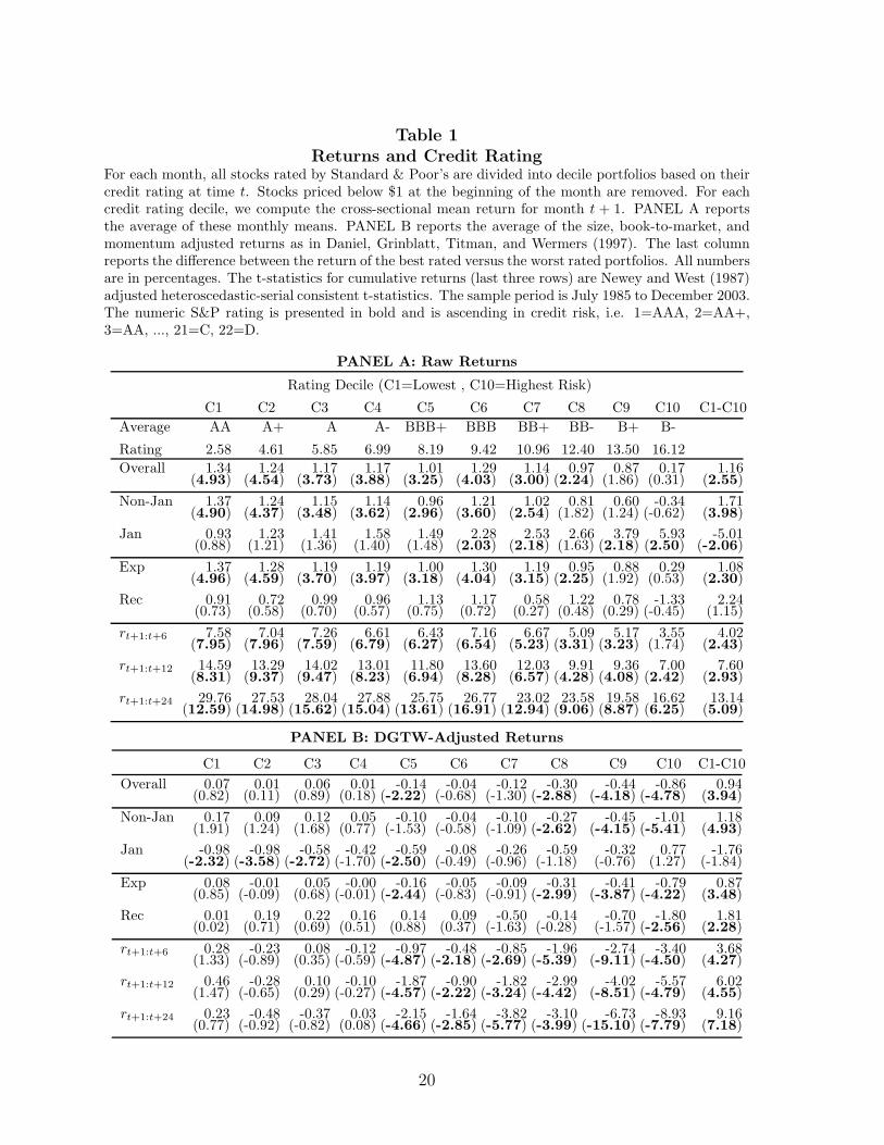
Table 1Returns and Credit Rating

For each month, all stocks rated by Standard & Poor’s are divided into decile portfolios based on theircredit rating at time t. Stocks priced below $1 at the beginning of the month are removed. For eachcredit rating decile, we compute the cross-sectional mean return for month t + 1. PANEL A reportsthe average of these monthly means. PANEL B reports the average of the size, book-to-market, andmomentum adjusted returns as in Daniel, Grinblatt, Titman, and Wermers (1997). The last columnreports the difference between the return of the best rated versus the worst rated portfolios. All numbersare in percentages. The t-statistics for cumulative returns (last three rows) are Newey and West (1987)adjusted heteroscedastic-serial consistent t-statistics. The sample period is July 1985 to December 2003.The numeric S&P rating is presented in bold and is ascending in credit risk, i.e. 1=AAA, 2=AA+,3=AA, ..., 21=C, 22=D.

PANEL A: Raw Returns

Rating Decile (C1=Lowest , C10=Highest Risk)

C1 C2 C3 C4 C5 C6 C7 C8 C9 C10 C1-C10Average AA A+ A A- BBB+ BBB BB+ BB- B+ B-

Rating 2.58 4.61 5.85 6.99 8.19 9.42 10.96 12.40 13.50 16.12Overall 1.34 1.24 1.17 1.17 1.01 1.29 1.14 0.97 0.87 0.17 1.16

(4.93) (4.54) (3.73) (3.88) (3.25) (4.03) (3.00) (2.24) (1.86) (0.31) (2.55)Non-Jan 1.37 1.24 1.15 1.14 0.96 1.21 1.02 0.81 0.60 -0.34 1.71

(4.90) (4.37) (3.48) (3.62) (2.96) (3.60) (2.54) (1.82) (1.24) (-0.62) (3.98)Jan 0.93 1.23 1.41 1.58 1.49 2.28 2.53 2.66 3.79 5.93 -5.01

(0.88) (1.21) (1.36) (1.40) (1.48) (2.03) (2.18) (1.63) (2.18) (2.50) (-2.06)Exp 1.37 1.28 1.19 1.19 1.00 1.30 1.19 0.95 0.88 0.29 1.08

(4.96) (4.59) (3.70) (3.97) (3.18) (4.04) (3.15) (2.25) (1.92) (0.53) (2.30)Rec 0.91 0.72 0.99 0.96 1.13 1.17 0.58 1.22 0.78 -1.33 2.24

(0.73) (0.58) (0.70) (0.57) (0.75) (0.72) (0.27) (0.48) (0.29) (-0.45) (1.15)rt+1:t+6 7.58 7.04 7.26 6.61 6.43 7.16 6.67 5.09 5.17 3.55 4.02

(7.95) (7.96) (7.59) (6.79) (6.27) (6.54) (5.23) (3.31) (3.23) (1.74) (2.43)rt+1:t+12 14.59 13.29 14.02 13.01 11.80 13.60 12.03 9.91 9.36 7.00 7.60

(8.31) (9.37) (9.47) (8.23) (6.94) (8.28) (6.57) (4.28) (4.08) (2.42) (2.93)rt+1:t+24 29.76 27.53 28.04 27.88 25.75 26.77 23.02 23.58 19.58 16.62 13.14

(12.59) (14.98) (15.62) (15.04) (13.61) (16.91) (12.94) (9.06) (8.87) (6.25) (5.09)

PANEL B: DGTW-Adjusted Returns

C1 C2 C3 C4 C5 C6 C7 C8 C9 C10 C1-C10Overall 0.07 0.01 0.06 0.01 -0.14 -0.04 -0.12 -0.30 -0.44 -0.86 0.94

(0.82) (0.11) (0.89) (0.18) (-2.22) (-0.68) (-1.30) (-2.88) (-4.18) (-4.78) (3.94)Non-Jan 0.17 0.09 0.12 0.05 -0.10 -0.04 -0.10 -0.27 -0.45 -1.01 1.18

(1.91) (1.24) (1.68) (0.77) (-1.53) (-0.58) (-1.09) (-2.62) (-4.15) (-5.41) (4.93)Jan -0.98 -0.98 -0.58 -0.42 -0.59 -0.08 -0.26 -0.59 -0.32 0.77 -1.76

(-2.32) (-3.58) (-2.72) (-1.70) (-2.50) (-0.49) (-0.96) (-1.18) (-0.76) (1.27) (-1.84)Exp 0.08 -0.01 0.05 -0.00 -0.16 -0.05 -0.09 -0.31 -0.41 -0.79 0.87

(0.85) (-0.09) (0.68) (-0.01) (-2.44) (-0.83) (-0.91) (-2.99) (-3.87) (-4.22) (3.48)Rec 0.01 0.19 0.22 0.16 0.14 0.09 -0.50 -0.14 -0.70 -1.80 1.81

(0.02) (0.71) (0.69) (0.51) (0.88) (0.37) (-1.63) (-0.28) (-1.57) (-2.56) (2.28)rt+1:t+6 0.28 -0.23 0.08 -0.12 -0.97 -0.48 -0.85 -1.96 -2.74 -3.40 3.68

(1.33) (-0.89) (0.35) (-0.59) (-4.87) (-2.18) (-2.69) (-5.39) (-9.11) (-4.50) (4.27)rt+1:t+12 0.46 -0.28 0.10 -0.10 -1.87 -0.90 -1.82 -2.99 -4.02 -5.57 6.02

(1.47) (-0.65) (0.29) (-0.27) (-4.57) (-2.22) (-3.24) (-4.42) (-8.51) (-4.79) (4.55)rt+1:t+24 0.23 -0.48 -0.37 0.03 -2.15 -1.64 -3.82 -3.10 -6.73 -8.93 9.16

(0.77) (-0.92) (-0.82) (0.08) (-4.66) (-2.85) (-5.77) (-3.99) (-15.10) (-7.79) (7.18)

20

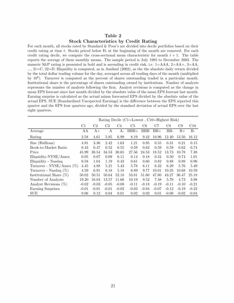
Table 2Stock Characteristics by Credit Rating

For each month, all stocks rated by Standard & Poor’s are divided into decile portfolios based on theircredit rating at time t. Stocks priced below $1 at the beginning of the month are removed. For eachcredit rating decile, we compute the cross-sectional mean characteristic for month t + 1. The tablereports the average of these monthly means. The sample period is July 1985 to December 2003. Thenumeric S&P rating is presented in bold and is ascending in credit risk, i.e. 1=AAA, 2=AA+, 3=AA,..., 21=C, 22=D. Illiquidity is computed, as in Amihud (2002), as the the absolute daily return dividedby the total dollar trading volume for the day, averaged across all trading days of the month (multipliedby 106). Turnover is computed as the percent of shares outstanding traded in a particular month.Institutional share is the percentage of shares outstanding owned by institutions. Number of analystsrepresents the number of analysts following the firm. Analyst revisions is computed as the change inmean EPS forecast since last month divided by the absolute value of the mean EPS forecast last month.Earning surprise is calculated as the actual minus forecasted EPS divided by the absolute value of theactual EPS. SUE [Standardized Unexpected Earnings] is the difference between the EPS reported thisquarter and the EPS four quarters ago, divided by the standard deviation of actual EPS over the lasteight quarters.


C1 C2 C3 C4 C5 C6 C7 C8 C9 C10Average AA A+ A A- BBB+ BBB BB+ BB- B+ B-

Rating 2.58 4.61 5.85 6.99 8.19 9.42 10.96 12.40 13.50 16.12

Size ($billions) 4.91 3.36 2.42 1.63 1.21 0.95 0.55 0.31 0.21 0.15Book-to-Market Ratio 0.43 0.47 0.52 0.55 0.59 0.62 0.59 0.59 0.62 0.74Price 45.99 38.54 34.53 30.65 27.56 24.53 18.52 13.73 10.78 7.38Illiquidity-NYSE/Amex 0.05 0.07 0.09 0.11 0.14 0.18 0.34 0.50 0.74 1.01Illiquidity - Nasdaq 0.58 1.04 1.19 0.43 0.61 0.60 0.82 0.88 0.89 0.96Turnover - NYSE/Amex (%) 4.45 4.88 5.21 5.43 5.78 6.11 6.32 6.29 5.76 5.49Turnover - Nasdaq (%) 4.59 6.91 6.18 5.18 6.89 9.77 10.01 10.35 10.68 10.59Institutional Share (%) 50.02 50.51 50.64 52.18 53.81 51.60 47.80 43.27 36.47 25.18Number of Analysts 19.20 16.04 13.57 11.66 10.19 9.52 7.48 5.70 4.73 3.98Analyst Revisions (%) -0.02 -0.03 -0.05 -0.08 -0.11 -0.18 -0.19 -0.11 -0.10 -0.21Earning Surprises -0.01 -0.01 -0.01 -0.02 -0.03 -0.04 -0.07 -0.12 -0.19 -0.22SUE 0.06 0.12 0.04 0.01 0.02 0.02 0.01 -0.00 -0.02 -0.04

21

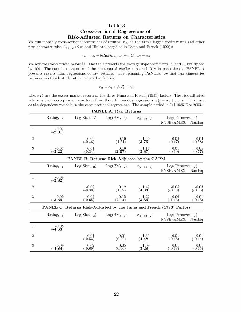
Table 3Cross-Sectional Regressions of

Risk-Adjusted Returns on CharacteristicsWe run monthly cross-sectional regressions of returns, rit, on the firm’s lagged credit rating and otherfirm characteristics, Ci,t−2 (Size and BM are lagged as in Fama and French (1992)):

rit = at + btRatingi,t−1 + ctCi,t−2 + uit

We remove stocks priced below $1. The table presents the average slope coefficients, bt and ct, multipliedby 100. The sample t-statistics of these estimated coefficients are below in parentheses. PANEL Apresents results from regressions of raw returns. The remaining PANELs, we first run time-seriesregressions of each stock return on market factors:

rit = αi + βiFt + eit

where Ft are the excess market return or the three Fama and French (1993) factors. The risk-adjustedreturn is the intercept and error term from these time-series regressions: r∗it = αi + eit, which we useas the dependent variable in the cross-sectional regressions. The sample period is Jul 1985-Dec 2003.

PANEL A: Raw Returns

Ratingt−1 Log(Sizet−2) Log(BMt−2) r(t−7:t−2) Log(Turnovert−2)NYSE/AMEX Nasdaq

1 -0.07(-2.01)

2 -0.02 0.10 1.40 0.04 0.04(-0.46) (1.51) (3.75) (0.47) (0.58)

3 -0.07 0.01 0.16 1.17 0.01 0.05(-2.22) (0.34) (2.07) (2.87) (0.19) (0.77)

PANEL B: Returns Risk-Adjusted by the CAPM


1 -0.09(-2.82)

2 -0.02 0.12 1.42 -0.05 -0.03(-0.39) (1.89) (4.33) (-0.88) (-0.55)

3 -0.09 -0.02 0.15 1.22 -0.06 -0.01(-3.55) (-0.65) (2.14) (3.35) (-1.15) (-0.13)

PANEL C: Returns Risk-Adjusted by the Fama and French (1993) Factors


1 -0.08(-4.63)

2 -0.01 0.01 1.31 0.01 -0.01(-0.53) (0.22) (4.48) (0.18) (-0.14)

3 -0.09 -0.02 0.05 1.09 -0.01 0.01(-4.84) (-0.60) (0.96) (3.28) (-0.13) (0.15)

22

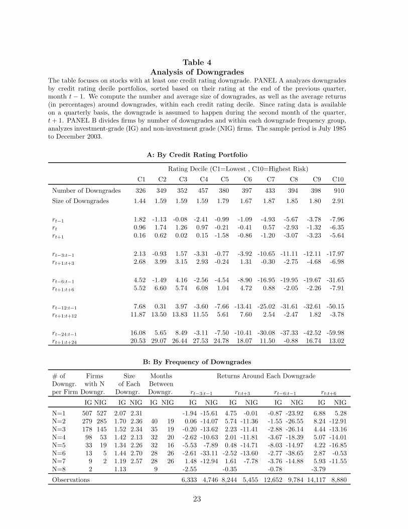
Table 4Analysis of Downgrades

The table focuses on stocks with at least one credit rating downgrade. PANEL A analyzes downgradesby credit rating decile portfolios, sorted based on their rating at the end of the previous quarter,month t − 1. We compute the number and average size of downgrades, as well as the average returns(in percentages) around downgrades, within each credit rating decile. Since rating data is availableon a quarterly basis, the downgrade is assumed to happen during the second month of the quarter,t + 1. PANEL B divides firms by number of downgrades and within each downgrade frequency group,analyzes investment-grade (IG) and non-investment grade (NIG) firms. The sample period is July 1985to December 2003.

A: By Credit Rating Portfolio


C1 C2 C3 C4 C5 C6 C7 C8 C9 C10

Number of Downgrades 326 349 352 457 380 397 433 394 398 910

Size of Downgrades 1.44 1.59 1.59 1.59 1.79 1.67 1.87 1.85 1.80 2.91

rt−1 1.82 -1.13 -0.08 -2.41 -0.99 -1.09 -4.93 -5.67 -3.78 -7.96rt 0.96 1.74 1.26 0.97 -0.21 -0.41 0.57 -2.93 -1.32 -6.35rt+1 0.16 0.62 0.02 0.15 -1.58 -0.86 -1.20 -3.07 -3.23 -5.64

rt−3:t−1 2.13 -0.93 1.57 -3.31 -0.77 -3.92 -10.65 -11.11 -12.11 -17.97rt+1:t+3 2.68 3.99 3.15 2.93 -0.24 1.31 -0.30 -2.75 -4.68 -6.98

rt−6:t−1 4.52 -1.49 4.16 -2.56 -4.54 -8.90 -16.95 -19.95 -19.67 -31.65rt+1:t+6 5.52 6.60 5.74 6.08 1.04 4.72 0.88 -2.05 -2.26 -7.91

rt−12:t−1 7.68 0.31 3.97 -3.60 -7.66 -13.41 -25.02 -31.61 -32.61 -50.15rt+1:t+12 11.87 13.50 13.83 11.55 5.61 7.60 2.54 -2.47 1.82 -3.78

rt−24:t−1 16.08 5.65 8.49 -3.11 -7.50 -10.41 -30.08 -37.33 -42.52 -59.98rt+1:t+24 20.53 29.07 26.44 27.53 24.78 18.07 11.50 -0.88 16.74 13.02

B: By Frequency of Downgrades

# of Firms Size Months Returns Around Each DowngradeDowngr. with N of Each Betweenper Firm Downgr. Downgr. Downgr. rt−3:t−1 rt:t+3 rt−6:t−1 rt:t+6

IG NIG IG NIG IG NIG IG NIG IG NIG IG NIG IG NIG

N=1 507 527 2.07 2.31 -1.94 -15.61 4.75 -0.01 -0.87 -23.92 6.88 5.28N=2 279 285 1.70 2.36 40 19 0.06 -14.07 5.74 -11.36 -1.55 -26.55 8.24 -12.91N=3 178 145 1.52 2.34 35 19 -0.20 -13.62 2.23 -11.41 -2.88 -26.14 4.44 -13.16N=4 98 53 1.42 2.13 32 20 -2.62 -10.63 2.01 -11.81 -3.67 -18.39 5.07 -14.01N=5 33 19 1.34 2.26 32 16 -5.53 -7.89 0.48 -14.71 -8.03 -14.97 4.22 -16.85N=6 13 5 1.44 2.70 28 26 -2.61 -33.11 -2.52 -13.60 -2.77 -38.65 2.87 -0.53N=7 9 2 1.19 2.57 28 26 1.48 -12.94 1.61 -7.78 -3.76 -14.88 5.93 -11.55N=8 2 1.13 9 -2.55 -0.35 -0.78 -3.79

Observations 6,333 4,746 8,244 5,455 12,652 9,784 14,117 8,880

23

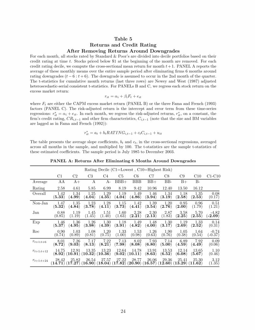
Table 5Returns and Credit Rating

After Removing Returns Around DowngradesFor each month, all stocks rated by Standard & Poor’s are divided into decile portfolios based on theircredit rating at time t. Stocks priced below $1 at the beginning of the month are removed. For eachcredit rating decile, we compute the cross-sectional mean return for month t+1. PANEL A reports theaverage of these monthly means over the entire sample period after eliminating firms 6 months aroundrating downgrades (t− 6 : t + 6). The downgrade is assumed to occur in the 2nd month of the quarter.The t-statistics for cumulative month returns (last three rows) are Newey and West (1987) adjustedheteroscedastic-serial consistent t-statistics. For PANELs B and C, we regress each stock return on theexcess market return:

rit = αi + βiFt + eit

where Ft are either the CAPM excess market return (PANEL B) or the three Fama and French (1993)factors (PANEL C). The risk-adjusted return is the intercept and error term from these time-seriesregressions: r∗it = αi + eit. In each month, we regress the risk-adjusted returns, r∗it, on a constant, thefirm’s credit rating, CRi,t−1 and other firm characteristics, Ci,t−1 (note that the size and BM variablesare lagged as in Fama and French (1992)):

r∗it = at + btRATINGi,t−1 + ctCi,t−1 + uit

The table presents the average slope coefficients, bt and ct, in the cross-sectional regressions, averagedacross all months in the sample, and multiplied by 100. The t-statistics are the sample t-statistics ofthese estimated coefficients. The sample period is July 1985 to December 2003.

PANEL A: Returns After Eliminating 6 Months Around Downgrades


C1 C2 C3 C4 C5 C6 C7 C8 C9 C10 C1-C10Average AA A+ A A- BBB+ BBB BB+ BB- B+ B-

Rating 2.58 4.61 5.85 6.99 8.19 9.42 10.96 12.40 13.50 16.12Overall 1.42 1.34 1.25 1.29 1.19 1.49 1.46 1.34 1.18 1.35 0.08

(5.33) (4.99) (4.04) (4.35) (4.04) (4.86) (3.94) (3.19) (2.58) (2.53) (0.17)Non-Jan 1.47 1.35 1.23 1.28 1.15 1.42 1.39 1.20 0.95 0.96 0.51

(5.32) (4.84) (3.78) (4.11) (3.73) (4.41) (3.54) (2.76) (2.00) (1.79) (1.21)Jan 0.88 1.19 1.45 1.51 1.60 2.28 2.30 2.87 3.58 5.70 -4.82

(0.85) (1.19) (1.45) (1.40) (1.63) (2.21) (2.13) (1.83) (2.25) (2.55) (-2.09)Exp 1.46 1.36 1.26 1.30 1.18 1.49 1.48 1.30 1.19 1.33 0.14

(5.37) (4.95) (3.98) (4.39) (3.91) (4.82) (4.00) (3.17) (2.69) (2.52) (0.31)Rec 0.90 1.03 1.08 1.20 1.33 1.53 1.26 1.90 1.05 1.64 -0.74

(0.74) (0.89) (0.81) (0.75) (1.00) (0.98) (0.63) (0.76) (0.38) (0.54) (-0.37)rt+1:t+6 8.01 7.26 7.17 7.22 7.13 8.02 7.93 7.14 6.89 7.92 0.09

(8.72) (9.03) (8.13) (8.21) (7.98) (8.08) (6.80) (5.00) (4.59) (4.49) (0.06)rt+1:t+12 14.75 12.91 13.35 13.23 12.64 14.78 13.91 13.53 12.14 13.65 1.10

(8.92) (10.91) (10.32) (10.36) (9.02) (10.11) (8.63) (6.52) (6.08) (5.67) (0.46)rt+1:t+24 28.42 25.82 26.54 27.57 27.22 28.77 26.06 29.36 25.41 25.30 3.12

(14.71) (17.27) (16.90) (18.04) (17.82) (20.90) (16.57) (12.60) (13.29) (11.62) (1.35)

24

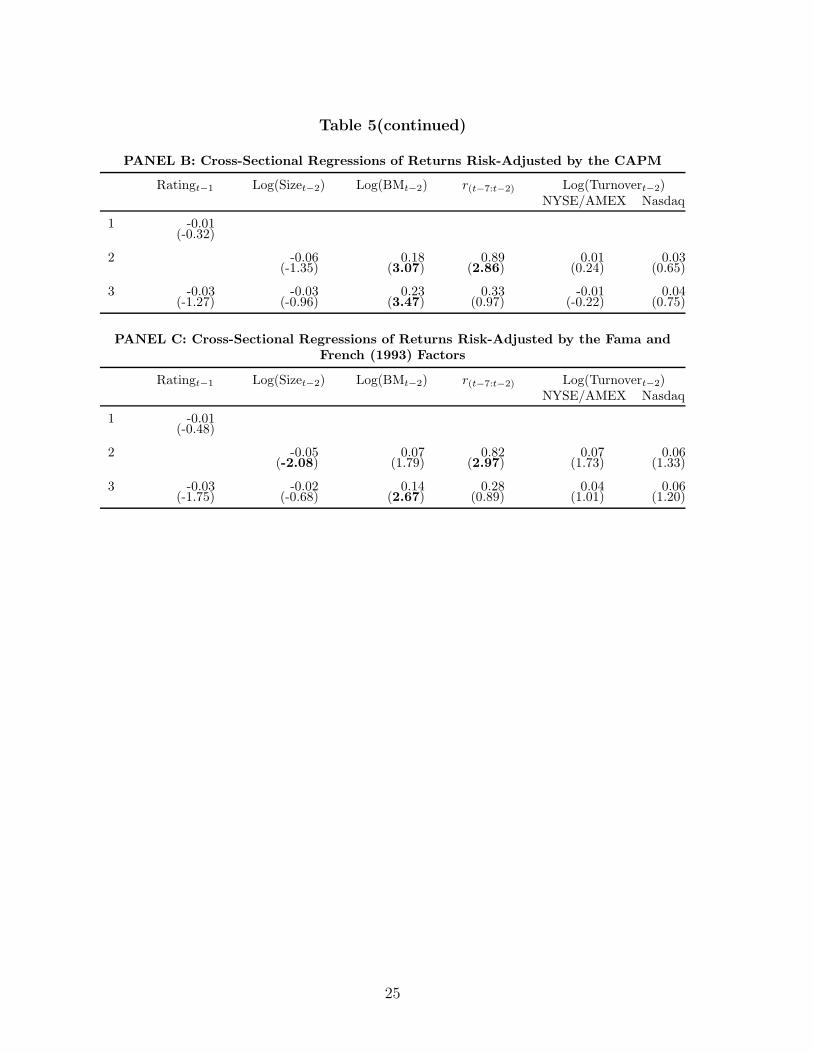
Table 5(continued)

PANEL B: Cross-Sectional Regressions of Returns Risk-Adjusted by the CAPM


1 -0.01(-0.32)

2 -0.06 0.18 0.89 0.01 0.03(-1.35) (3.07) (2.86) (0.24) (0.65)

3 -0.03 -0.03 0.23 0.33 -0.01 0.04(-1.27) (-0.96) (3.47) (0.97) (-0.22) (0.75)

PANEL C: Cross-Sectional Regressions of Returns Risk-Adjusted by the Fama andFrench (1993) Factors


1 -0.01(-0.48)

2 -0.05 0.07 0.82 0.07 0.06(-2.08) (1.79) (2.97) (1.73) (1.33)

3 -0.03 -0.02 0.14 0.28 0.04 0.06(-1.75) (-0.68) (2.67) (0.89) (1.01) (1.20)

25

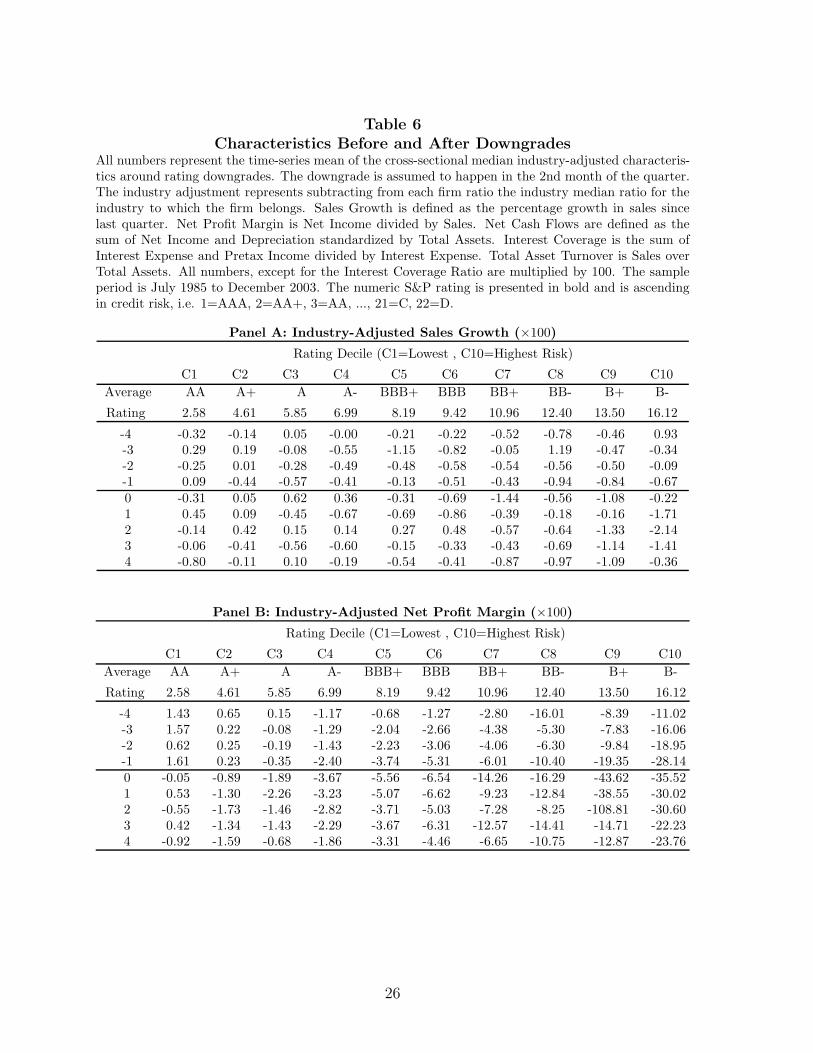
Table 6Characteristics Before and After Downgrades

All numbers represent the time-series mean of the cross-sectional median industry-adjusted characteris-tics around rating downgrades. The downgrade is assumed to happen in the 2nd month of the quarter.The industry adjustment represents subtracting from each firm ratio the industry median ratio for theindustry to which the firm belongs. Sales Growth is defined as the percentage growth in sales sincelast quarter. Net Profit Margin is Net Income divided by Sales. Net Cash Flows are defined as thesum of Net Income and Depreciation standardized by Total Assets. Interest Coverage is the sum ofInterest Expense and Pretax Income divided by Interest Expense. Total Asset Turnover is Sales overTotal Assets. All numbers, except for the Interest Coverage Ratio are multiplied by 100. The sampleperiod is July 1985 to December 2003. The numeric S&P rating is presented in bold and is ascendingin credit risk, i.e. 1=AAA, 2=AA+, 3=AA, ..., 21=C, 22=D.

Panel A: Industry-Adjusted Sales Growth (×100)



Rating 2.58 4.61 5.85 6.99 8.19 9.42 10.96 12.40 13.50 16.12

-4 -0.32 -0.14 0.05 -0.00 -0.21 -0.22 -0.52 -0.78 -0.46 0.93-3 0.29 0.19 -0.08 -0.55 -1.15 -0.82 -0.05 1.19 -0.47 -0.34-2 -0.25 0.01 -0.28 -0.49 -0.48 -0.58 -0.54 -0.56 -0.50 -0.09-1 0.09 -0.44 -0.57 -0.41 -0.13 -0.51 -0.43 -0.94 -0.84 -0.670 -0.31 0.05 0.62 0.36 -0.31 -0.69 -1.44 -0.56 -1.08 -0.221 0.45 0.09 -0.45 -0.67 -0.69 -0.86 -0.39 -0.18 -0.16 -1.712 -0.14 0.42 0.15 0.14 0.27 0.48 -0.57 -0.64 -1.33 -2.143 -0.06 -0.41 -0.56 -0.60 -0.15 -0.33 -0.43 -0.69 -1.14 -1.414 -0.80 -0.11 0.10 -0.19 -0.54 -0.41 -0.87 -0.97 -1.09 -0.36

Panel B: Industry-Adjusted Net Profit Margin (×100)



Rating 2.58 4.61 5.85 6.99 8.19 9.42 10.96 12.40 13.50 16.12

-4 1.43 0.65 0.15 -1.17 -0.68 -1.27 -2.80 -16.01 -8.39 -11.02-3 1.57 0.22 -0.08 -1.29 -2.04 -2.66 -4.38 -5.30 -7.83 -16.06-2 0.62 0.25 -0.19 -1.43 -2.23 -3.06 -4.06 -6.30 -9.84 -18.95-1 1.61 0.23 -0.35 -2.40 -3.74 -5.31 -6.01 -10.40 -19.35 -28.140 -0.05 -0.89 -1.89 -3.67 -5.56 -6.54 -14.26 -16.29 -43.62 -35.521 0.53 -1.30 -2.26 -3.23 -5.07 -6.62 -9.23 -12.84 -38.55 -30.022 -0.55 -1.73 -1.46 -2.82 -3.71 -5.03 -7.28 -8.25 -108.81 -30.603 0.42 -1.34 -1.43 -2.29 -3.67 -6.31 -12.57 -14.41 -14.71 -22.234 -0.92 -1.59 -0.68 -1.86 -3.31 -4.46 -6.65 -10.75 -12.87 -23.76

26

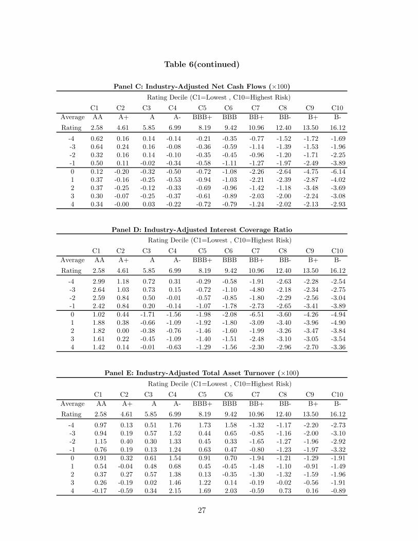
Table 6(continued)

Panel C: Industry-Adjusted Net Cash Flows (×100)



Rating 2.58 4.61 5.85 6.99 8.19 9.42 10.96 12.40 13.50 16.12

-4 0.62 0.16 0.14 -0.14 -0.21 -0.35 -0.77 -1.52 -1.72 -1.69-3 0.64 0.24 0.16 -0.08 -0.36 -0.59 -1.14 -1.39 -1.53 -1.96-2 0.32 0.16 0.14 -0.10 -0.35 -0.45 -0.96 -1.20 -1.71 -2.25-1 0.50 0.11 -0.02 -0.34 -0.58 -1.11 -1.27 -1.97 -2.49 -3.890 0.12 -0.20 -0.32 -0.50 -0.72 -1.08 -2.26 -2.64 -4.75 -6.141 0.37 -0.16 -0.25 -0.53 -0.94 -1.03 -2.21 -2.39 -2.87 -4.022 0.37 -0.25 -0.12 -0.33 -0.69 -0.96 -1.42 -1.18 -3.48 -3.693 0.30 -0.07 -0.25 -0.37 -0.61 -0.89 -2.03 -2.00 -2.24 -3.084 0.34 -0.00 0.03 -0.22 -0.72 -0.79 -1.24 -2.02 -2.13 -2.93

Panel D: Industry-Adjusted Interest Coverage Ratio



Rating 2.58 4.61 5.85 6.99 8.19 9.42 10.96 12.40 13.50 16.12

-4 2.99 1.18 0.72 0.31 -0.29 -0.58 -1.91 -2.63 -2.28 -2.54-3 2.64 1.03 0.73 0.15 -0.72 -1.10 -4.80 -2.18 -2.34 -2.75-2 2.59 0.84 0.50 -0.01 -0.57 -0.85 -1.80 -2.29 -2.56 -3.04-1 2.42 0.84 0.20 -0.14 -1.07 -1.78 -2.73 -2.65 -3.41 -3.890 1.02 0.44 -1.71 -1.56 -1.98 -2.08 -6.51 -3.60 -4.26 -4.941 1.88 0.38 -0.66 -1.09 -1.92 -1.80 -3.09 -3.40 -3.96 -4.902 1.82 0.00 -0.38 -0.76 -1.46 -1.60 -1.99 -3.26 -3.47 -3.843 1.61 0.22 -0.45 -1.09 -1.40 -1.51 -2.48 -3.10 -3.05 -3.544 1.42 0.14 -0.01 -0.63 -1.29 -1.56 -2.30 -2.96 -2.70 -3.36

Panel E: Industry-Adjusted Total Asset Turnover (×100)



Rating 2.58 4.61 5.85 6.99 8.19 9.42 10.96 12.40 13.50 16.12

-4 0.97 0.13 0.51 1.76 1.73 1.58 -1.32 -1.17 -2.20 -2.73-3 0.94 0.19 0.57 1.52 0.44 0.65 -0.85 -1.16 -2.00 -3.10-2 1.15 0.40 0.30 1.33 0.45 0.33 -1.65 -1.27 -1.96 -2.92-1 0.76 0.19 0.13 1.24 0.63 0.47 -0.80 -1.23 -1.97 -3.320 0.91 0.32 0.61 1.54 0.91 0.70 -1.94 -1.21 -1.29 -1.911 0.54 -0.04 0.48 0.68 0.45 -0.45 -1.48 -1.10 -0.91 -1.492 0.37 0.27 0.57 1.38 0.13 -0.35 -1.30 -1.32 -1.59 -1.963 0.26 -0.19 0.02 1.46 1.22 0.14 -0.19 -0.02 -0.56 -1.914 -0.17 -0.59 0.34 2.15 1.69 2.03 -0.59 0.73 0.16 -0.89

27

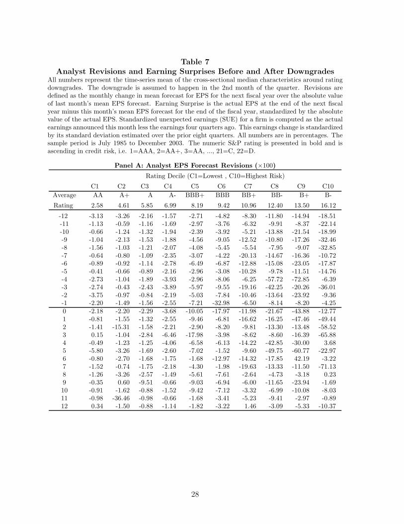
Table 7Analyst Revisions and Earning Surprises Before and After Downgrades

All numbers represent the time-series mean of the cross-sectional median characteristics around ratingdowngrades. The downgrade is assumed to happen in the 2nd month of the quarter. Revisions aredefined as the monthly change in mean forecast for EPS for the next fiscal year over the absolute valueof last month’s mean EPS forecast. Earning Surprise is the actual EPS at the end of the next fiscalyear minus this month’s mean EPS forecast for the end of the fiscal year, standardized by the absolutevalue of the actual EPS. Standardized unexpected earnings (SUE) for a firm is computed as the actualearnings announced this month less the earnings four quarters ago. This earnings change is standardizedby its standard deviation estimated over the prior eight quarters. All numbers are in percentages. Thesample period is July 1985 to December 2003. The numeric S&P rating is presented in bold and isascending in credit risk, i.e. 1=AAA, 2=AA+, 3=AA, ..., 21=C, 22=D.

Panel A: Analyst EPS Forecast Revisions (×100)



Rating 2.58 4.61 5.85 6.99 8.19 9.42 10.96 12.40 13.50 16.12

-12 -3.13 -3.26 -2.16 -1.57 -2.71 -4.82 -8.30 -11.80 -14.94 -18.51-11 -1.13 -0.59 -1.16 -1.69 -2.97 -3.76 -6.32 -9.91 -8.37 -22.14-10 -0.66 -1.24 -1.32 -1.94 -2.39 -3.92 -5.21 -13.88 -21.54 -18.99-9 -1.04 -2.13 -1.53 -1.88 -4.56 -9.05 -12.52 -10.80 -17.26 -32.46-8 -1.56 -1.03 -1.21 -2.07 -4.08 -5.45 -5.54 -7.95 -9.07 -32.85-7 -0.64 -0.80 -1.09 -2.35 -3.07 -4.22 -20.13 -14.67 -16.36 -10.72-6 -0.89 -0.92 -1.14 -2.78 -6.49 -6.87 -12.88 -15.08 -23.05 -17.87-5 -0.41 -0.66 -0.89 -2.16 -2.96 -3.08 -10.28 -9.78 -11.51 -14.76-4 -2.73 -1.04 -1.89 -3.93 -2.96 -8.06 -6.25 -57.72 -72.85 -6.39-3 -2.74 -0.43 -2.43 -3.89 -5.97 -9.55 -19.16 -42.25 -20.26 -36.01-2 -3.75 -0.97 -0.84 -2.19 -5.03 -7.84 -10.46 -13.64 -23.92 -9.36-1 -2.20 -1.49 -1.56 -2.55 -7.21 -32.98 -6.50 -8.14 -8.20 -4.250 -2.18 -2.20 -2.29 -3.68 -10.05 -17.97 -11.98 -21.67 -43.88 -12.771 -0.81 -1.55 -1.32 -2.55 -9.46 -6.81 -16.62 -16.25 -47.46 -49.442 -1.41 -15.31 -1.58 -2.21 -2.90 -8.20 -9.81 -13.30 -13.48 -58.523 0.15 -1.04 -2.84 -6.46 -17.98 -3.98 -8.62 -8.60 -16.39 -65.884 -0.49 -1.23 -1.25 -4.06 -6.58 -6.13 -14.22 -42.85 -30.00 3.685 -5.80 -3.26 -1.69 -2.60 -7.02 -1.52 -9.60 -49.75 -60.77 -22.976 -0.80 -2.70 -1.68 -1.75 -1.68 -12.97 -14.32 -17.85 42.19 -3.227 -1.52 -0.74 -1.75 -2.18 -4.30 -1.98 -19.63 -13.33 -11.50 -71.138 -1.26 -3.26 -2.57 -1.49 -5.61 -7.61 -2.64 -4.73 -3.18 0.239 -0.35 0.60 -9.51 -0.66 -9.03 -6.94 -6.00 -11.65 -23.94 -1.6910 -0.91 -1.62 -0.88 -1.52 -9.42 -7.12 -3.32 -6.99 -10.08 -8.0311 -0.98 -36.46 -0.98 -0.66 -1.68 -3.41 -5.23 -9.41 -2.97 -0.8912 0.34 -1.50 -0.88 -1.14 -1.82 -3.22 1.46 -3.09 -5.33 -10.37

28

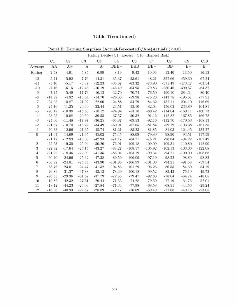
Table 7(continued)

Panel B: Earning Surprises (Actual-Forecasted)/Abs(Actual) (×100)



Rating 2.58 4.61 5.85 6.99 8.19 9.42 10.96 12.40 13.50 16.12

-12 -5.71 -5.92 -7.76 -14.31 -35.37 -53.61 -48.21 -357.66 -459.30 -67.24-11 -5.40 -5.17 -6.87 -12.23 -38.67 -63.32 -73.90 -375.49 -473.47 -63.54-10 -7.16 -6.15 -12.43 -16.19 -45.49 -64.95 -79.83 -250.46 -390.67 -64.37-9 -7.25 -5.49 -17.73 -16.12 -32.70 -70.74 -76.50 -190.10 -284.34 -80.40-8 -14.92 -4.82 -15.54 -14.70 -26.63 -59.98 -75.23 -143.78 -195.51 -77.21-7 -24.95 -10.87 -21.92 -22.00 -24.88 -54.79 -84.62 -157.11 -204.10 -116.69-6 -24.16 -11.25 -20.40 -22.44 -23.51 -53.10 -82.04 -156.02 -233.89 -164.81-5 -20.12 -10.38 -18.63 -18.12 -24.94 -53.18 -89.42 -114.04 -169.11 -160.73-4 -23.25 -10.08 -20.50 -39.55 -67.57 -50.32 -91.12 -112.82 -167.85 -166.78-3 -24.06 -11.48 -17.97 -36.25 -63.87 -69.53 -92.16 -112.70 -170.53 -168.13-2 -21.67 -10.70 -16.22 -34.49 -60.91 -67.65 -81.84 -59.79 -103.38 -161.35-1 -20.33 -12.96 -21.35 -45.74 -81.21 -83.23 -81.85 -81.03 -124.45 -132.270 -21.64 -14.69 -21.65 -45.02 -75.45 -88.09 -79.89 -98.90 -93.51 -117.591 -21.17 -12.89 -19.39 -42.93 -71.17 -84.71 -75.21 -98.64 -94.22 -107.492 -25.53 -19.30 -25.94 -50.20 -76.91 -109.18 -109.09 -109.31 -110.80 -112.903 -22.92 -17.64 -25.15 -43.27 -88.27 -108.57 -105.92 -102.13 -103.06 -122.084 -21.22 -18.46 -22.90 -41.35 -86.04 -103.19 -99.34 -94.71 -100.00 -108.685 -60.40 -24.96 -25.32 -47.38 -89.59 -106.09 -97.19 -98.52 -98.89 -98.826 -56.82 -24.01 -24.54 -43.90 -101.96 -106.99 -101.03 -94.21 -91.58 -59.547 -33.76 -23.01 -24.47 -41.52 -104.86 -101.29 -96.26 -86.55 -84.60 -54.198 -26.89 -31.37 -37.88 -43.13 -78.39 -100.18 -99.52 -83.43 -76.19 -49.739 -26.65 -29.36 -31.67 -37.79 -72.55 -79.47 -92.83 -78.04 -64.74 -48.0510 -19.82 -42.32 -27.31 -29.44 -71.55 -74.28 -79.59 -77.19 -64.76 -52.0111 -18.12 -44.23 -26.03 -27.84 -71.34 -77.98 -68.58 -68.51 -44.56 -29.2412 -16.96 -40.93 -22.57 -28.89 -72.17 -76.09 -59.49 -71.68 -40.16 -23.05

29

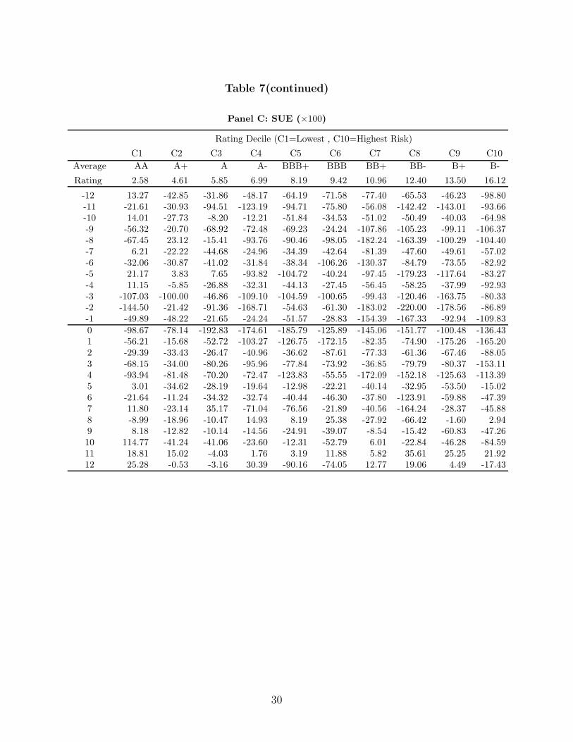
Table 7(continued)

Panel C: SUE (×100)



Rating 2.58 4.61 5.85 6.99 8.19 9.42 10.96 12.40 13.50 16.12

-12 13.27 -42.85 -31.86 -48.17 -64.19 -71.58 -77.40 -65.53 -46.23 -98.80-11 -21.61 -30.93 -94.51 -123.19 -94.71 -75.80 -56.08 -142.42 -143.01 -93.66-10 14.01 -27.73 -8.20 -12.21 -51.84 -34.53 -51.02 -50.49 -40.03 -64.98-9 -56.32 -20.70 -68.92 -72.48 -69.23 -24.24 -107.86 -105.23 -99.11 -106.37-8 -67.45 23.12 -15.41 -93.76 -90.46 -98.05 -182.24 -163.39 -100.29 -104.40-7 6.21 -22.22 -44.68 -24.96 -34.39 -42.64 -81.39 -47.60 -49.61 -57.02-6 -32.06 -30.87 -41.02 -31.84 -38.34 -106.26 -130.37 -84.79 -73.55 -82.92-5 21.17 3.83 7.65 -93.82 -104.72 -40.24 -97.45 -179.23 -117.64 -83.27-4 11.15 -5.85 -26.88 -32.31 -44.13 -27.45 -56.45 -58.25 -37.99 -92.93-3 -107.03 -100.00 -46.86 -109.10 -104.59 -100.65 -99.43 -120.46 -163.75 -80.33-2 -144.50 -21.42 -91.36 -168.71 -54.63 -61.30 -183.02 -220.00 -178.56 -86.89-1 -49.89 -48.22 -21.65 -24.24 -51.57 -28.83 -154.39 -167.33 -92.94 -109.830 -98.67 -78.14 -192.83 -174.61 -185.79 -125.89 -145.06 -151.77 -100.48 -136.431 -56.21 -15.68 -52.72 -103.27 -126.75 -172.15 -82.35 -74.90 -175.26 -165.202 -29.39 -33.43 -26.47 -40.96 -36.62 -87.61 -77.33 -61.36 -67.46 -88.053 -68.15 -34.00 -80.26 -95.96 -77.84 -73.92 -36.85 -79.79 -80.37 -153.114 -93.94 -81.48 -70.20 -72.47 -123.83 -55.55 -172.09 -152.18 -125.63 -113.395 3.01 -34.62 -28.19 -19.64 -12.98 -22.21 -40.14 -32.95 -53.50 -15.026 -21.64 -11.24 -34.32 -32.74 -40.44 -46.30 -37.80 -123.91 -59.88 -47.397 11.80 -23.14 35.17 -71.04 -76.56 -21.89 -40.56 -164.24 -28.37 -45.888 -8.99 -18.96 -10.47 14.93 8.19 25.38 -27.92 -66.42 -1.60 2.949 8.18 -12.82 -10.14 -14.56 -24.91 -39.07 -8.54 -15.42 -60.83 -47.2610 114.77 -41.24 -41.06 -23.60 -12.31 -52.79 6.01 -22.84 -46.28 -84.5911 18.81 15.02 -4.03 1.76 3.19 11.88 5.82 35.61 25.25 21.9212 25.28 -0.53 -3.16 30.39 -90.16 -74.05 12.77 19.06 4.49 -17.43

30

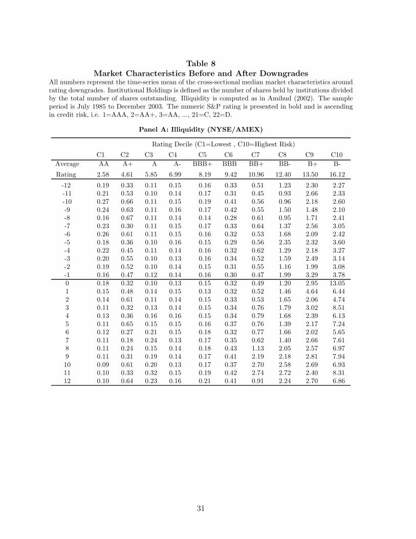
Table 8Market Characteristics Before and After Downgrades

All numbers represent the time-series mean of the cross-sectional median market characteristics aroundrating downgrades. Institutional Holdings is defined as the number of shares held by institutions dividedby the total number of shares outstanding. Illiquidity is computed as in Amihud (2002). The sampleperiod is July 1985 to December 2003. The numeric S&P rating is presented in bold and is ascendingin credit risk, i.e. 1=AAA, 2=AA+, 3=AA, ..., 21=C, 22=D.

Panel A: Illiquidity (NYSE/AMEX)



Rating 2.58 4.61 5.85 6.99 8.19 9.42 10.96 12.40 13.50 16.12

-12 0.19 0.33 0.11 0.15 0.16 0.33 0.51 1.23 2.30 2.27-11 0.21 0.53 0.10 0.14 0.17 0.31 0.45 0.93 2.66 2.33-10 0.27 0.66 0.11 0.15 0.19 0.41 0.56 0.96 2.18 2.60-9 0.24 0.63 0.11 0.16 0.17 0.42 0.55 1.50 1.48 2.10-8 0.16 0.67 0.11 0.14 0.14 0.28 0.61 0.95 1.71 2.41-7 0.23 0.30 0.11 0.15 0.17 0.33 0.64 1.37 2.56 3.05-6 0.26 0.61 0.11 0.15 0.16 0.32 0.53 1.68 2.09 2.42-5 0.18 0.36 0.10 0.16 0.15 0.29 0.56 2.35 2.32 3.60-4 0.22 0.45 0.11 0.14 0.16 0.32 0.62 1.29 2.18 3.27-3 0.20 0.55 0.10 0.13 0.16 0.34 0.52 1.59 2.49 3.14-2 0.19 0.52 0.10 0.14 0.15 0.31 0.55 1.16 1.99 3.08-1 0.16 0.47 0.12 0.14 0.16 0.30 0.47 1.99 3.29 3.780 0.18 0.32 0.10 0.13 0.15 0.32 0.49 1.20 2.95 13.051 0.15 0.48 0.14 0.15 0.13 0.32 0.52 1.46 4.64 6.442 0.14 0.61 0.11 0.14 0.15 0.33 0.53 1.65 2.06 4.743 0.11 0.32 0.13 0.14 0.15 0.34 0.76 1.79 3.02 8.514 0.13 0.36 0.16 0.16 0.15 0.34 0.79 1.68 2.39 6.135 0.11 0.65 0.15 0.15 0.16 0.37 0.76 1.39 2.17 7.246 0.12 0.27 0.21 0.15 0.18 0.32 0.77 1.66 2.02 5.657 0.11 0.18 0.24 0.13 0.17 0.35 0.62 1.40 2.66 7.618 0.11 0.24 0.15 0.14 0.18 0.43 1.13 2.05 2.57 6.979 0.11 0.31 0.19 0.14 0.17 0.41 2.19 2.18 2.81 7.9410 0.09 0.61 0.20 0.13 0.17 0.37 2.70 2.58 2.69 6.9311 0.10 0.33 0.32 0.15 0.19 0.42 2.74 2.72 2.40 8.3112 0.10 0.64 0.23 0.16 0.21 0.41 0.91 2.24 2.70 6.86

31

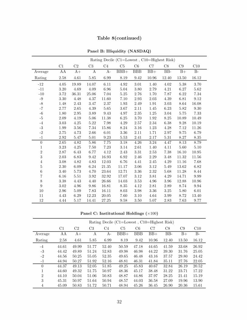
Table 8(continued)

Panel B: Illiquidity (NASDAQ)



Rating 2.58 4.61 5.85 6.99 8.19 9.42 10.96 12.40 13.50 16.12

-12 4.05 19.89 14.07 6.11 4.92 3.01 1.40 4.02 5.38 3.70-11 3.20 4.69 4.09 6.96 5.04 3.80 2.79 4.21 6.27 5.62-10 3.72 36.31 25.06 7.04 5.25 2.76 1.70 7.87 6.22 7.34-9 3.30 4.48 4.37 11.60 7.10 2.93 2.03 4.39 6.81 9.12-8 1.48 2.43 3.47 2.37 1.93 2.49 1.91 3.03 8.64 16.08-7 2.77 2.65 4.39 5.65 3.67 2.11 1.45 6.23 5.82 9.30-6 1.80 2.95 3.89 9.43 4.97 2.35 1.25 3.04 5.75 7.33-5 2.09 4.19 5.06 11.38 6.25 3.70 1.92 8.25 10.89 10.49-4 3.03 4.25 5.22 7.98 4.29 2.57 2.34 6.38 9.28 10.19-3 1.99 3.56 7.34 15.86 8.24 3.16 1.23 4.28 7.12 11.26-2 2.75 4.73 2.66 6.01 3.36 2.11 1.71 2.97 9.75 6.79-1 2.92 5.47 5.01 9.23 5.53 2.41 2.17 5.31 8.27 8.350 2.65 4.82 5.86 7.75 3.18 4.26 3.24 4.47 8.13 8.791 3.23 4.25 7.50 7.23 3.14 2.61 1.40 4.11 5.60 5.102 2.87 6.43 6.77 4.12 2.43 3.31 2.53 7.38 16.10 10.953 2.03 6.83 9.42 16.93 6.92 2.46 2.29 3.48 11.32 11.564 3.08 4.82 4.83 12.03 6.76 4.41 2.45 4.29 11.16 7.685 2.30 6.09 6.24 21.35 11.17 3.06 3.12 5.49 13.62 6.826 3.40 5.73 4.70 23.64 12.71 3.36 2.32 5.68 11.28 8.447 6.16 5.51 3.92 32.92 17.07 3.12 3.81 4.29 14.71 9.998 3.38 4.43 4.40 26.66 14.03 3.53 4.96 3.96 12.88 10.969 3.02 4.96 9.86 16.81 8.35 4.12 2.81 2.89 8.74 9.9410 2.96 5.09 7.83 16.11 8.03 3.98 3.36 3.25 5.80 6.0111 4.43 6.29 12.23 20.05 7.60 3.10 4.64 3.99 8.72 13.4012 4.44 5.17 14.41 27.25 9.58 3.50 5.07 2.83 7.63 9.77

Panel C: Institutional Holdings (×100)



Rating 2.58 4.61 5.85 6.99 8.19 9.42 10.96 12.40 13.50 16.12

-4 44.61 49.99 51.77 52.40 50.59 47.18 44.65 41.59 33.68 26.92-3 44.42 49.89 51.24 52.83 49.98 46.98 44.22 39.30 31.76 25.05-2 44.56 50.25 55.05 52.35 49.65 46.48 43.16 37.57 29.80 24.42-1 44.94 50.27 51.92 52.16 48.81 46.31 41.84 35.11 27.76 22.050 44.37 49.13 52.05 51.85 49.25 45.83 40.67 32.84 26.19 20.521 44.60 49.32 51.75 50.97 48.36 45.17 38.48 31.22 23.71 17.222 44.10 50.04 51.06 50.83 48.87 44.86 37.97 28.25 21.41 15.193 45.31 50.97 51.64 50.94 48.57 44.03 36.58 27.09 19.96 13.904 45.09 50.83 51.72 50.71 48.94 45.26 36.45 26.90 20.36 15.61

32

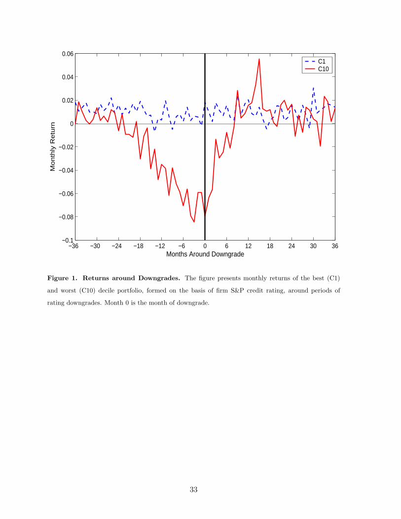
−36 −30 −24 −18 −12 −6 0 6 12 18 24 30 36−0.1

−0.08

−0.06

−0.04

−0.02

0

0.02

0.04

0.06

Months Around Downgrade

Month

ly R

etu

rnC1C10

Figure 1. Returns around Downgrades. The figure presents monthly returns of the best (C1)

and worst (C10) decile portfolio, formed on the basis of firm S&P credit rating, around periods of

rating downgrades. Month 0 is the month of downgrade.

33

Documents

Credit Ratings and The Cross-Section of Stock Returns