THE HEAT RADIATION DIFFUSION EQUATION Explicit Analytical ...thermalscience.vinca.rs/pdfs/papers-2018/TSCI171011308H.pdf · Hristov, J.,: The Heat Radiation Diffusion Equation: Explicit

Hristov, J.,: The Heat Radiation Diffusion Equation: Explicit Analytical Solutions ... THERMAL SCIENCE: Year 2018, Vol. 22, No. 2, pp. 777-788 777

THE HEAT RADIATION DIFFUSION EQUATION Explicit Analytical Solutions by Improved Integral-Balance Method

by

Jordan HRISTOV*

Department of Chemical Engineering, University of Chemical Technology and Metallurgy, Sofia, Bulgaria

Original scientific paper https://doi.org/10.2298/TSCI171011308H

Approximate explicit analytical solutions of the heat radiation diffusion equation by applying the double integration technique of the integral-balance method have been developed. The method allows approximate closed form solutions to be devel-oped. A problem with a step change of the surface temperature and two problems with time dependent boundary conditions have been solved. The error minimiza-tion of the approximate solutions has been developed straightforwardly by minimi-zation of the residual function of the governing equation.

Introduction

Heat wave behavior of thermal diffusion due to radiation is a reasonable physical and mathematic interpretation of thermal energy transfer in a variety of applied problem related to astrophysical phenomena [1], plasma physics [2, 3], building insulation [4], etc. In general, this physical model assumes a diffusion approximation relating the local thermal flux at any point of the medium by the local gradient of the radiation energy density that is an approach known from the classical Fourier law. Following Smith [5] the 1-D energy transfer by radiation and absence of fluid motion is:

et x

Φρ ∂ ∂= −

∂ ∂,

443

TK x

σΦρ∂

= −∂

(1)

The presentation of the thermal flux density, Φ , as a gradient of the 4th power of the local temperature is an accordance with the Rosseland approximation [1, 5, 6] which is valid for thick, non-opaque media in absence of fluid motion [5-9].

The diffusion eq. (1) was solved for the first time by Barenblatt [10] by a self-similar solution and then refined by Zeldovich and Raizer [11]. As commented by Smith [5] these early attempts, especially the report of Hammer and Rosen [12] repeated the idea of the Barenblatt but met problems in defining the shape of the spatial temperature distribution profile. At the same time as the Barenblatt solution appeared the study of Marshak [9] was carried out (performed in 1944-1945 in Los Alamos Laboratory, N. Mex., USA, but published only in 1958 as it is especially mentioned in the publication). The Marshak solution also tried to express the spatial temperature distribution as a series of parabolic profiles. We will especially consider this model in the article since the new method used applies a generalized parabolic profile. For further deep reading on the solutions related to radiation-diffusion equation we refer to [5-8] and the references therein.

Author e-mail: [email protected]

Hristov, J.,: The Heat Radiation Diffusion Equation: Explicit Analytical Solutions ... 778 THERMAL SCIENCE: Year 2018, Vol. 22, No. 2, pp. 777-788

The aim of the present work is to present an approximate closed form analytical solu-tion allowing to estimate the penetration depth of the heat wave and the spatial temperature distribution applying an improved integral-balance approach [13, 14] already successfully ap-plied to non-linear heat conduction problems modelled by degenerate parabolic equations (see further in the text).

The non-linear heat radiation diffusion equation

In accordance with Smith [5] the internal energy, e , and Rosseland mean opacity, K , are approximated by power-law of temperature, T , and density, ρ , as:

Te fβ

µρ= , 1 Tg

K

α

λρ= (2)

where f = 3.4 [MJkg–1] and g = 1/7200 [gcm–2] are dimensional constants (especially for the case of gold) [12].

The exponents α and β are positive constants and in accordance with [5] and [12] we have 1.5α = and 1.6β = . With the power-laws (2) the energy balance (1) yields the follow-ing diffusion equation:

2 4

2

T TDt x

β α+∂ ∂=

∂ ∂, 2

163

gDf µ λ

ε σβ ρ − += ,

4βεα

=+

(3)

It is noteworthy that the dimension of the diffusion coefficient, D , in eq. (3) is [ ]42m /sK α β+ − and only in the case when 0α = and 1β = we have 2 3[m /sK ]D ≡ .

Smith [5] used the parameter 4U T α β+ −= to transform eq. (3) into a wave equation:

2 2

2

11

U U U UDt x xε ε

∂ ∂ ∂ = + ∂ − ∂ ∂ (4)

Equation (4) excludes the case 1ε ≠ corresponding to the linear diffusion model. The transformed eq. (4) was solved by Smith [5] with a series approximation:

( ) ( )1

, ii

iU z t c t z

∞

=

= ∑ , Fz x x= − (5)

In the context of the Smith solution Fx defines the front of a heat wave beyond which the medium is undisturbed, i. e. 0T = for Fx x≥ that is ( )0, 0U t = . To this point, we will stop considering the Smith solution but will refer to it in comments on results developed in this article.

Solution approach

Integral balance approach in brief

The integral-balance method used in this work is based on the concept that the diffu-sant (heat or mass) penetrates the undisturbed medium at a final depth ( )tδ which evolves in time. Therefore, the common boundary conditions at infinity ( ) 0T ∞ = and ( ), 0T t x∂ ∞ ∂ = can be replaced by:

( ) 0T δ = and ( ) 0Txδ∂

=∂

(6)

The conditions (6) define a sharp-front movement ( )tδ of the boundary between dis-turbed and undisturbed medium. The position ( )tδ is unknown and should be determined trough


the solution. When the classical heat diffusion problem is at issue and the thermal diffusivity is temperature-independent (i. e. 0 constanta a= = ) [13-15]:

( ) 2

0 2

,T x t Tat x

∂ ∂=

∂ ∂ (7)

The integration of eq. (7) over a finite penetration depth, δ , and applying the Leibniz rule for differentiation under the integral sign results in eq. (8):

( ) ( )00

d , d 0,d

TT x t x a tt x

δ ∂= −

∂∫ (8)

or equivalently:

( ) ( ) ( )00

, ,d d 0,

x

x

T x t T x t Tx x a tt t x

δ∂ ∂ ∂+ = −

∂ ∂ ∂∫ ∫ (9)

Physically, eq. (8), as well as eq. (9) imply that the total thermal energy accumulated into the finite layer (from 0x = to x δ= ) is balanced by the heat flux at the interface 0x = . Equations (8) and (9) are the principle relationships of the simplest version of the integral-bal-ance method known as heat-balance integral method (HBIM) [16]. After this first step, replac-ing T by an assumed profile aT (expressed as a function of the relative space co-ordinate /x δ ), then the integration in eq. (8) results in an ODE about ( )tδ [13, 14, 16, 17]. The principle drawback of eq. (8) is that the right-side depends on gradient expressed through the type of the assumed profile.

An improvement, avoiding the drawback of HBIM is the double integration method (DIM) [13, 14]. The first step of DIM is integration of from 0 to x , namely:

( ) ( ) ( )0 0

0

, , 0,d

x T x t T x t T tx a a

t x x∂ ∂ ∂

= −∂ ∂ ∂∫ (10)

Subtracting eq. (10) from eq. (9) we get:

( ) ( )0

, ,d

x

T x t T x tx a

t x

δ ∂ ∂=

∂ ∂∫ (11)

Equation (11) has the same physical meaning as eq. (8). The integration of eq. (11) from 0 to δ results in:

( )00

d d 0,x

T x x a T tt

δ δ ∂=

∂ ∫ ∫ (12)

The integral relation of eq. (12) allows to work with either integer-order time-deriv-atives (as in the present case) or with time-fractional derivatives [19] where the Leibniz rule is inapplicable.

If the thermal diffusivity is non-linear and expressed as a power-law mpa a T= ( 0m > ),

corresponding to degenerate diffusion problems, then eq. (12) takes the form [13, 14]:

( ) 1

0

d d 0,1

mp

x

aT x x T tt m

δ δ+ ∂

= ∂ + ∫ ∫ (13)


The integral relation (13) will be used further in this work in the solutions of the problems at issue.

Transformation of the governing equation and degenerate diffusion equation

Here, following the notations of Smith [5] in section The non-linear heat radiation diffusion equation and denoting T βθ = which leads to 1T βθ= and ( )44T α βα θ ++ = . Now, we can present eq. (3):

2

2

w

Dt xθ θ∂ ∂=

∂ ∂, 4w α

β+

= (14)

From eq. (14) it is obvious that 1 wε = defined in eq. (3). From the defined values of α and β we have that 1w > . Equation (14) can be presented as [13]:

mwD

t x xθ θθ∂ ∂ ∂ = ∂ ∂ ∂

, 11

1

mm

x m xθ θθ

+∂ ∂=

∂ + ∂ (15)

where wD wD= and 1 0m w= − > .The transformed eq. (15) allows direct application of the DIM, as it is demonstrated

next. This is a classical example of the so-called slow diffusion models [19, 20] which degenerates at 0θ = , that is at the front of the moving solution. A change of variables mϕ θ= and t mτ = allows eqs. (15) to be expressed:

2 2

2wD mx x

ϕ ϕ ϕϕτ

∂ ∂ ∂ = + ∂ ∂ ∂ (16)

Equation (16) has the same structure as eq. (4) solved by Smith [5] and reveals a superposition of non-linear wave propagation and diffusion and it was successfully solved by HBIM in [15].

The DIM solutions: constant density cases

Step change of temperature at the boundary

This example only demonstrates the technique of DIM applicable to the radiation diffusion equation and how the approximate profile should be determined. For the sake of sim-plicity a Dirichlet (a step change in the boundary condition at 0x = ) is considered to eq. (15).

The application of DIM to eq. (15) yields the following integral relations (equivalent) to (13), namely:

( ) ( )0

0,d , d dd 1

m

wx

tx t x x D

t m

δ δ θθ =

+∫ ∫ (17)

For Dirichlet boundary condition constantsT = we have ( )0, constants st T βθ θ= = = . The DIM solution assumes an approximate profile as parabolic one with unspecified exponent

(1 / )ns xθ θ δ= − which satisfies the boundary conditions (6) for any positive value of the expo-

nent n [13, 21]. Applying DIM we get:

( )( )( )

DIM

1 21w wD

n nD t

mδ

+ +=

+ (18)


Then, the normalized approximate solution is [13]:

( )( )

11 2

1

n

sw

xn n

D tm

θθ

Θ = = − + +

+

(19)

Thus defining the Boltzmann similarity variable 1/2/( )D wx D tη = . With the inverse change of variables 1T βθ= and 1

s sT βθ= we get:

( )( )norm 1

1 21

n

sw

T xTT n n

D tm

β = = − + +

+

(20)

As it was established in [13], the exponent n of the solution eq. (19) follows the rule 1/n m= and therefore, the profile (20) has an exponent equal to 1/mβ . Consequently with

1 4 1 3m w= − = − = , and 1.6β = we have 1/ 0.208mβ ≈ and the normalized solution is:

( )

1

0.208

norm

2

1 10.4401 2

1

m

D DTm

m m

β

η η

= − = − + +

(21a,b)

Hence, for 1/2/( ) 0.440D wx D tη = = we have norm 0T = and this point defines the front of the heat wave.

Even though, HBIM and DIM are not self-similar method of solution, the benefits of their application is the definition of the dimensionless space co-ordinate /x δ allowing to deter-mine straightforwardly the desired similarity variable without preliminarily scaling of the mod-elling equation. This approach will be demonstrated effectively in the examples solved in the next points.

Temperature-independent properties with time dependent boundary condition (Marshak’s problem)

Marshak’s approach

Following Marshak [9], when the material density does not vary and the medium just heats up, the equation takes the form (in the original notations) resembling eq. (14):

( )

2 4

24

pMDT T

t p x

+∂ ∂=

∂ + ∂, 04

3MclD = (22)

The pseudo-diffusion coefficient, MD , has a dimension 3 3[m /sK ]p+ as it was demon-strated in eq. (3). Marshak [9] considered time dependent boundary condition: 0 exp(2 )s sT J tα= ,

0x = , where 0J is the initial surface temperature at 0t = and sα is a time constant. The solution was developed as a series 00( ) (1 / )i

if z A z z∞== −∑ , with the ansatzes of eqs. (23).


( )1

3

0

1pzf z A

z

+ = −

, ( )

00 0

312p

A zJ L

+= ,

( )

320

0 02

3

pLz Jp

+ =

+, 0

0 23 M

s

clL Dα

= = (23)

Here 0z defines the front of the thermal wave. Marshak detected that only one term is enough to assure approximation error of 1.2%, if 3p = . Hence, with 3p = assumed by Marshak we have 1/( 3) 1 6 0.166p + = ≈ , 0 0 03 /A z J L= , 3

0 0 0 /3z J L= and the normalized solution of Mar-shak is:

( ) ( )0.166

30 0 0

0 0

133

f z f z zz J LA

J L

= = −

(24)

The DIM solution

The application of DIM from (13)-(22) with (1 / )na sT T x δ= − , with ( )s sT T t= yields:

( )

( ) ( )2

400

d exp 2, exp 2

dps

M s

J tD N n p J t

tα δ

α+ = , ( ) ( )( )

( )1 2

,4

n nN n p

p+ +

=+

(25)

From eq. (25) with ( 0) 0tδ = = we have:

( ) ( )( )

2 330

,2 4

st ppM

s

N n pD J ep

αδα

++=+

(26)

The product 30 /p

M sD J α+ has a dimension [m2] and therefore the ratio 3 1/20/ [( / ) ]p

M sx D Jα + is dimensionless. Hence, the normalized approximate solution is:

( )( )2

0

,1

,2

s

n

a Mt

T x tJ e N n pα

η = −

, ( )2 33

0 e s

Mt ppM

s

xD J α

η

α++

= (27a,b)

This solution defines the similarity variable Mη (27b), while the denominator of (27a) defines numerically the penetration depth.

The residual function of eq. (22) is a measure of the error of approximation when the approximate solution is used. Following the methodology used in [13, 14] we have:

( )1 4 2

2

4 4 11 d 1 1d

n nMD n nx x xR n

tδ

δ δ δ δ δ

− −− = − − −

(28)

If R should be zero at the interface 0x = , satisfying eqs. (22), then from eq. (28) it follows that 4 1 0 1/4n n− = → = . Otherwise, the requirement (0, ) 0R t > should be satisfied if

1/4n < . At the front of the thermal-layer when x δ→ , the last term of eq. (28) tells us that the condition 4 2 0 1/2n n− > → > should be obeyed. However, the first condition established at

0x = is more important since it allows determining the flux at the boundary. Moreover R can be presented as 2( , )/R r z t δ= [13], where with /z x δ= we may present the expanding in time thermal-layer as a fixed boundary domain since 0 1z≤ ≤ . Hence, ( , )r z t is:


( ) ( ) ( )( )2

1 4 21 d, 1 4 4 1 12 d

n nMr z t z n z D n n z

tδ − −= − − − − (29)

Then, the mean squared error of approximation over the thermal-layer is δ (i. e. from 0z = to 1z = ) is:

( ) ( ) ( )1 1

2 2

40 0

1, , d , dE z t R z t z r z t zδ

= = ∫ ∫ (30)

Since, ( , )E z t decays in time with a speed proportional to 41/δ it is important to min-imize it at the beginning of the diffusion process. Then, following Myers [22] and setting 0t = in all time-dependent terms we get:

( )( ) 2

4 4 1,0

8 1n n

E zn− =−

(31)

Hence, we get a minimal error of approximation at 0t = for 1/4n = which coincides with the value established earlier at 0x = . Moreover, from the denominator of ( ,0)E z it follows that 1/8n > , a condition satisfied by 1/4n = . However, this exponent is not the exact one [22]. Moreover, as it was reported in [12] the profile 1 4(1 / )s FT T x x≈ − is the solution of the steady-state equation 2 4 2/ 0T x∂ ∂ = , with Fx is the optical depth to the heat front.

Now, we recall that eq. (22) can be presented:

qM

T TD Tt x x

∂ ∂ ∂ = ∂ ∂ ∂ , 3q p= + (32)

This is a well-known degenerate diffusion equation [19-21]. As it was established in [13, 15] and mentioned in the preceding example, the exponent of the approximate profile can be approximated as 1/n q≈ . Then, with 1/( 3)n p= + we have ( , ) 2N n p = and 1/2[ ( , ) / 2] 1N n p = . Then, the normalized approximate profile is:

( ) ( )1

32

0

,1

s

a pMt

T x tJ e α η +

− ≈ − (33)

Hence, 1Mη = defines the front of the thermal-layer, that in dimensional form is:

( )2 330 e st ppM

s

Dx J αδ α

++= (34)

The penetration depth 0z in the solution of Marshak is defined through the surface temperature by (3 )/2

0pJ + and this confirms qualitatively the DIM solution where (3 )/2

0pJδ +≡ . In

most of cases the value of p is stipulated through the scaling exponents α and β in the ap-proximations such as eq. (2). The Marshak exponent 0.166n = satisfies the condition 1/8 0.166 1/4Mn< = < . The exponent 1/4n = corresponds to 1/( 3)n p= + for 1p = and this pro-vides 1/2[ ( , )] 1N n p = . Moreover, from (22) we get 4 5pT T+ ≈ . With 1β = in eq. (22) which is equivalent to eq. (14) we have (4 )/ 5.5w α β= + ≈ and a scaling 5.5wT T≈ .

Therefore, due to different formulations of the similarity variables and different solu-tion techniques we got different exponents of the approximating parabolic profile. In this con-text, the method determining the exponent through minimization of the means-squared error of


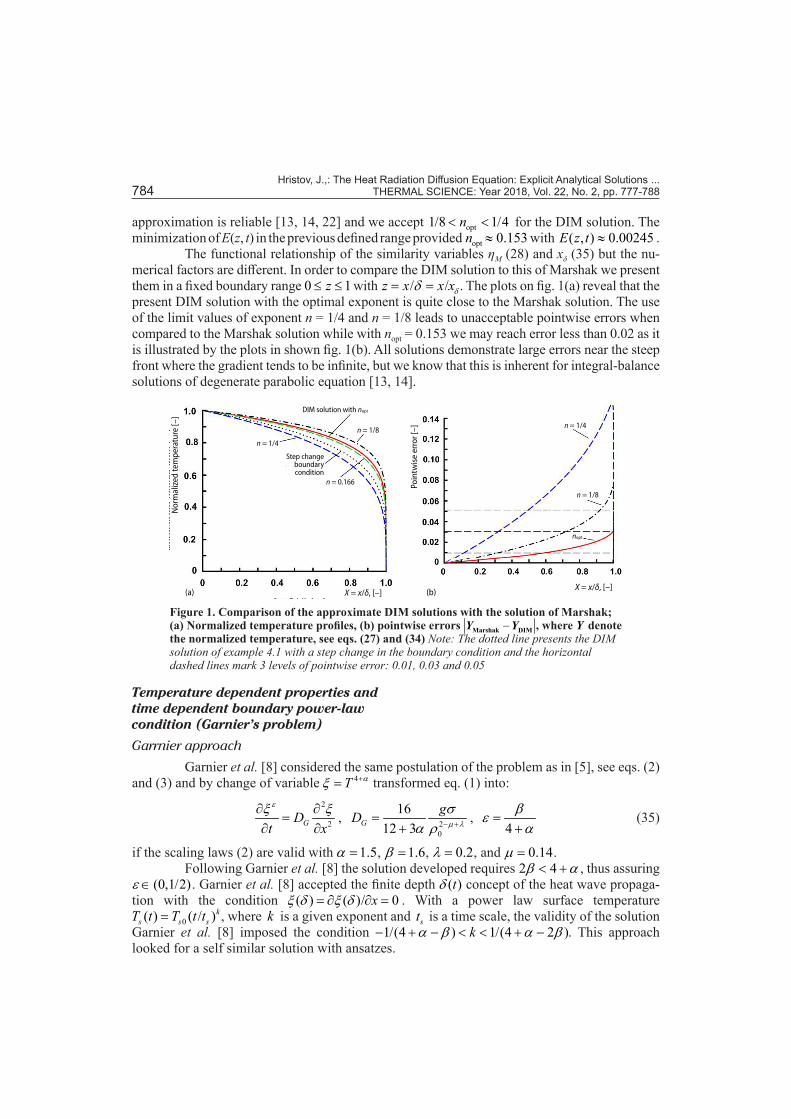
approximation is reliable [13, 14, 22] and we accept opt1/8 1/4n< < for the DIM solution. The minimization of E(z, t) in the previous defined range provided opt 0.153n ≈ with ( , ) 0.00245E z t ≈ .

The functional relationship of the similarity variables ηM (28) and xδ (35) but the nu-merical factors are different. In order to compare the DIM solution to this of Marshak we present them in a fixed boundary range 0 1z≤ ≤ with / /z x x xδδ= = . The plots on fig. 1(a) reveal that the present DIM solution with the optimal exponent is quite close to the Marshak solution. The use of the limit values of exponent n = 1/4 and n = 1/8 leads to unacceptable pointwise errors when compared to the Marshak solution while with nopt = 0.153 we may reach error less than 0.02 as it is illustrated by the plots in shown fig. 1(b). All solutions demonstrate large errors near the steep front where the gradient tends to be infinite, but we know that this is inherent for integral-balance solutions of degenerate parabolic equation [13, 14].

Figure 1. Comparison of the approximate DIM solutions with the solution of Marshak; (a) Normalized temperature profiles, (b) pointwise errors −Marshak DIMY Y , where Y denote the normalized temperature, see eqs. (27) and (34) Note: The dotted line presents the DIM solution of example 4.1 with a step change in the boundary condition and the horizontal dashed lines mark 3 levels of pointwise error: 0.01, 0.03 and 0.05

X = x/δ, [–]X = x/δ, [–]

Nor

mal

ized

tem

pera

ture

[–]

Poin

twis

e er

ror [

–]

(a) (b)

DIM solution with nopt

Step change boundary condition

n = 1/8

n = 1/4

n = 0.166

n = 1/8

n = 1/4

nopt

Temperature dependent properties and time dependent boundary power-law condition (Garnier’s problem)

Garrnier approach

Garnier et al. [8] considered the same postulation of the problem as in [5], see eqs. (2) and (3) and by change of variable 4T αξ += transformed eq. (1) into:

2

2GDt x

εξ ξ∂ ∂=

∂ ∂, 2

0

1612 3G

gD µ λ

σα ρ − +=

+,

4βεα

=+

(35)

if the scaling laws (2) are valid with 1.5α = , 1.6β = , 0.2λ = , and 0.14µ = . Following Garnier et al. [8] the solution developed requires 2 4β α< + , thus assuring

(0,1/2)ε ∈ . Garnier et al. [8] accepted the finite depth ( )tδ concept of the heat wave propaga-tion with the condition ( ) ( )/ 0xξ δ ξ δ= ∂ ∂ = . With a power law surface temperature

0( ) ( / )ks s sT t T t t= , where k is a given exponent and st is a time scale, the validity of the solution

Garnier et al. [8] imposed the condition 1/(4 ) 1/(4 2 )kα β α β− + − < < + − . This approach looked for a self similar solution with ansatzes.


( ) ( ) ( ), sx t t xξ ξ ξ δ= , ( ) ( ) 040

qs s st T t tαξ += , ( )0

Gnst tδ δ= ,

04q

kα+

= , 40 0G sD T αδ Γ += (36)

where Γ is a dimensionless parameter that parameterizes the differential equation about ξ . After substitution of (36) in (35) Garnier et al. [8] established that the exponent Gn

should be [1 (4 )]/2Gn k α β= + + − . Further, the solution was considered as an engeinvalue problem defining the eigenvalue-eigenfunction ( , )Γ ξ depending only on the values of α , β , and k . At this moment we stop the analysis of the solution of Garnier et al. [8] since it requires a numerical approach in contrast to the analytical DIM technique applied next.

The DIM solution

The change of the variable as 4Tε αθ ξ += = (as it was done in section Transformation of the governing equation and degenerate diffusion equation) transforms eq. (35):

2

2

w

GDt xθ θ∂ ∂=

∂ ∂, 4 1w α

β ε+

= = (37)

which is equivalent to eq .(14).With an assumed profile (1 / )n

s xθ θ δ= − and the DIM integral relationship (15) we get:

( ) ( )1

1 12 0,1

wk ws

Gts

N n w TD tkw a

δ−

− +=+

, ( ) ( )( )1 2,

n nN n w

w+ +

= , ( ) 1constant

kw

s tst a−= = (38)

Hence, the penetration depth is:

( ) ( )10

,Hw n

H G sts

N n wD T t

aδ −= , ( )4 1 1 1Hn k k wα β

β+ −

= + = − + (39a,b)

The DIM solution provides /2Hntδ ≡ and that ( 1) ( 1)/H Gn n β− = − . With 1.5α = and 1.6β = we have 1/2 1.218k

H tδ +≡ , while 1/2 1.95kG tδ +≡ . For 0k = both, Hδ and Gδ scale to 1/2t . Fur-

ther, with the inverse transforms 1/(4 )T αθ += the approximate solution ( , )aT x t is:

( ) 0, 1k q

a ss H

t xT x t Tt δ

= −

,

4nqα

=+

(40a,b)

The definition the residual function HR of eq. (37), carried out in a manner already demonstrated in section DIM solution, reveals that q should satisfy the condition 1/n w> and it is independent of k because the product ( 1) (d /d )w kt tδ δ− − emerging in expression of HR is time-independent. Then, the restriction on the exponent in eq. (40) is /(4 )q β α> + . If we sug-gest /(4 )q β α= + , then in eq. (40a) we should have 1n β= > which should provide an unphys-ical concave temperature profile of eq. (40a) as it was proved in [13, 14]. However, with the prescribed values of α and β we have 3.437w ≈ or 1 2.437m w= − = .

The optimization of the residual function with respect to q provides that for 2m = we have opt 0.666q ≈ , while for 3m = we have opt 0.640q ≈ . Now, from opt opt /(4 )q n α= + we

opt ( 2) 3.663n m = ≈ and opt ( 2) 3.520n m = ≈ . Precisely, for 2.437m = we get ( )opt 2.437 0.636mq = ≈ and consequently ( )opt 2.437 3.501mn = ≈ . Alternatively, if we suggest that the exponent q could be


expressed (4 )aq α+ it is easy to see that from the previous established values about optq we have ( )2 0.666a mq = ≈ and ( )3 0.640a mq = ≈ , while ( )2.437 0.649a mq = ≈ .

With these estimates, the normalized temperature profile is:

( )

( )

0.649

0

,1 2.684

1 4.347

a Hk

s ss

T x t

tT a kt

η ≈ − +

(41)

where 2 1/20/( )H Hn n

H G sx D T tη = is the similarity variable.The flux approximate profile follows directly from the definitions (1) and (35) and the

solution (41):

( )4 4 1

04, 1

k q

a G ss H H

t q xx t D Tt

Φδ δ

− = −

(42)

Mean while the approximated surface flux

4[ (0, )/ ]a G aD T t xΦ = − ∂ ∂ is 40[ ( / ) ] (4 / )k

a s s HT t t qΦ δ=

or in normalized form as 40/[ ( / ) ] (4 / )k

a s s HT t t qΦ δ= . From the results of eqs. (40a) and (40b) it follows that:

1 4 11 1.9524 4 2

4

0

k ka

k

ss

q t q ttTt

α ββΦ + − − + − +

≡ ≡

(43)

The normalized DIM solution, eq. (41), as a function of the similarity variable Hn is shown in fig. 2.

The condition of increasing surface flux when the surface temperature is prescribed as increasing power-law function of time follows from eq. (43) and the requirement is

7 /(4 ) 2.871k β α β< + − ≈ . Hence with linear or quadratic ramp of surface temperature the surface flux will increase in time. Moreover, the normalized flux follows from eq. (42):

( ) 4 1

4

0

,1

4

qa

kH

G ss H

x t x

t qD Tt

Φδ

δ

−

= −

(44)

This expression allows the present results to be compared at least qualitatively with the numerical solutions in [8]. For optimal

( )2.437 0.636a mq = ≈ we have 4 1 1.544 1q − ≈ > . With such an exponent the parabolic profile (44) generates concave distributions, see fig. 2, in contrast to temperature profiles which are convex.

Figure 2. The DIM solutions as normalized profiles of both the temperature and the heat flux with power-law time dependent boundary condition

X = x/δ, [–]

Nor

mal

ized

DIM

pro

file

[–] Temperature

Flux

q = 0.637

q = 0.666

q = 0.666q = 0.637


The approximate DIM temperature profile and the results of Garnier et al. [8] (numerical solutions) are hard to be compared due to incompatibility of the methods used. However, we have to mention that the developed DIM solution confirms the numerical results of Garnier et al., especially the profile in fig. 4 in [8], when the isothermal thermal shock condition were sim-ulated. To be precise, all examples discussed here are within the limit of the isothermal thermal shock as in the first postulation of Marshak [9]. Other regimes discussed in [8] such as subsonic waves and the ablation problem are out of the scope of the present work.

Conclusion

This work demonstrated the efficiency of the double-integration version of the inte-gral-balance method to solve the radiation diffusion equation. It was confirmed that this equa-tion can be easily presented as a degenerate parabolic equation. Then, the technique developed in [13] was efficiently applied to find explicit approximate and closed form solutions. The main differences between the solutions of Marshak and Garnier commented here and the DIM solu-tions are that in the former studies ansatzes about the penetration depth are used, while DIM defines such dimensionless groups (ansatzes) steps of the solutions. The second important step in the present solution is the optimization procedure defining the optimal exponent of the par-abolic profile [13]. This step, in fact, is application of the least squares method [23] since the entire function of the assumed parabolic profile is completely defined after determination of the penetration depth. Such procedure is not included in the previous solutions commented here.

References[1] Rosseland, S., Astrophysik und Atom-Theretische Grundlagen, Springer-Verlag, Berlin, 1931[2] Lonngren, K. E, et al., Field Penetration into Plasma with Nonlinear Conductivity, The Physics of Fluids,

17 (1974), 10, pp. 19191-1920[3] Broadbridge, P., et al., Non-Linear Heat Conduction through Externally Heated Radiant Plasma: Back-

ground Analysis for Numerical Study, J. Math Anal. Appl., 238 (1999), 2, pp. 353-368[4] Tilloua, A., et al., Dtermination of Physical Properties of Fibrous Thermal Insulation, EPJ Web of Con-

fernces, 33, (2012), 02009 [5] Smith, C. C., Solutions of the Radiation Diffusion Equation, High Energy Density Physics, 6 (2010), 1,

pp. 48-56[6] Clourt, J.-F., The Rosseland Approximation for Radiative Transfer Problems in Heterogeneous Media, J.

Quant. Specrosc. Radiat. Transfer, 58 (1997), 1, pp. 33-43[7] Magyari, E., Pantokratoras, A., Note on the Effect of Thermal Radiation in Linearized Rosseland Approx-

imation on Heat Transfer in Various Boundary Layer Flows, Int. Comm. Heat Mass Transfer, 38 (2011), 5, pp. 554-556

[8] Garnier, J., et al., Self-Similar Solution for Non-Linear Radiation Diffusion Equation, Phys. Plasmas, 13 (2006), 9, 092703

[9] Marshak, R. E., Effect of Radiation on Shock Wave Behaviour, The Physics of Fluids, 1 (1958), 1, pp. 24-29[10] Barenblatt, G. I., On Some Unsteady Motions of a Liquid or a Gas in a Porous Medium, App. Math.

Mech., 16 (1952), 1, pp. 67-78[11] Zeldovitch, Ya. B., Raizer, Yu. O., Physics of Shock Waves and High Temperature Hydrodynamic Phe-

nomena, Academic Press, New York, USA,1966[12] Hammer, J. H., Rosen, M. D., A Consistent Approach to Solving the Radiation Diffusion Equation, Phys.

Plasmas, 10 (2003), 5, 1829[13] Hristov, J., Integral Solutions to Transient Nonlinear Heat (Mass) Diffusion with a Power-Law Diffu-

sivity: A Semi-Infinite Medium with Fixed Boundary Conditions, Heat Mass Transfer, 52 (2016), 3, pp. 635-655

[14] Fabre, A., Hristov, J., On the Integral-Balance Approach to the Transient Heat Conduction with Linearly Temperature-Dependent Thermal Diffusivity, Heat Mass Transfer, 53 (2017), 1, pp. 177-204

[15] Hristov, J., An Approximate Analytical (Integral-Balance) Solution to A Nonlinear Heat Diffusion Equa-tion, Thermal Science, 19 (2015), 2, pp. 723-733


[16] Goodman, T. R., Application of Integral Methods to Transient Nonlinear Heat Transfer, in: Advances in Heat Transfer, (eds., T. F. Irvine and J. P. Hartnett, ), Vol. 1, 1964, Academic Press, San Diego, Cal., USA, pp. 51-122

[17] Hristov, J., The Heat-Balance Integral Method by a Parabolic Profile with Unspecified Exponent: Analy-sis and Benchmark Exercises, Thermal Science, 13 (2009), 2, pp. 27-48

[18] Hristov, J., Approximate Solutions to Time-Fractional Models by Integral Balance Approach, Chapter 5, in: Fractional Dynamics, (eds. C. Cattani, H. M. Srivastava, Xia-Jun Yang), De Gruyter Open, 2015, pp. 78-109.

[19] Hill, J. M., Similarity Solutions for Nonlinear Diffusion – A New Integration Procedure, J. Eng., Math., 23 (1989), 1, pp. 141-155

[20] Prasad, S. N., Salomon, H. B., A New Method for Analytical Solution of a Degenerate Diffusion Equation, Adv. Water Research, 28 (2005), 10, pp. 1091-1101

[21] Aronson, D. G., The Porous Medium Equation, in: Nonlinear Diffusion Problems, Lecture Notes in Math. 1224, (eds. A. Fasano and M. Primicerio), Springer-Verlag, Berlin, 1986, pp. 1-46

[22] Myers, T. G., Optimizing the Exponent in the Heat Balance and Refined Integral Methods, Int. Comm. Heat Mass Transfer, 36 (2009), 2, pp. 143-147

[23] Zwillinger, D., Handbook of Differential Equations, 3rd ed., Academic Press, New York, USA, 1997

Paper submitted: October 10, 2017Paper revised: November 13, 2017Paper accepted: November 13, 2017

© 2018 Society of Thermal Engineers of SerbiaPublished by the Vinča Institute of Nuclear Sciences, Belgrade, Serbia.

This is an open access article distributed under the CC BY-NC-ND 4.0 terms and conditions

Documents

THE HEAT RADIATION DIFFUSION EQUATION Explicit Analytical ...thermalscience.vinca.rs/pdfs/papers-2018/TSCI171011308H.pdf · Hristov, J.,: The Heat Radiation Diffusion Equation: Explicit