Vol. 44 (2013) ACTA PHYSICA POLONICA B No 5

RANDOM WALK, DIFFUSION AND WAVE EQUATION∗

Ryszard Wojnar

IPPT PAN — Institute of Fundamental Technological ResearchPolish Academy of Sciences

A. Pawińskiego 5b, 02-106 Warszawa, Poland

(Received May 20, 2013)

One-dimensional random walk is analyzed. First, it is shown that theclassical interpretation of random walk reaching Lord Rayleigh’s analysisshould be completed. Further, an attention is called to the fact that theparabolic diffusion is not an unique interpretation, but also the wave (orhyperbolic) equation can be deduced. It depends on the accepted scale ofthe length of step h and duration of the step τ in the walk, whether Fick–Smoluchowski’s diffusion or a wave process is obtained. Only additionalarguments, such as positivity of distribution function or positivity of theentropy growth, can help to choose the proper physical model. Also, theinfinite diffusion velocity paradox in connection with Einstein’s formula isexplained.

DOI:10.5506/APhysPolB.44.1067PACS numbers: 05.10.Gg, 05.40.Fb, 66.10.C–

1. Introduction

The concept of random walk was first introduced by Karl Pearson in1905 [1]. However, earlier in 1880, Lord Rayleigh applied this process (with-out naming it) to analyse a certain random vibration problem [2, 3].

Random walk is an idealisation of a path realised by a succession ofrandom steps, and can serve as a model for different stochastic processes.It is discussed in mathematics, physics, biology, economics and finance. Itmay denote the path traced by a Brownian particle as it travels in a liquid,the search path of a foraging animal and the stock fluctuating price, as well[4–15].

∗ Presented at the XXV Marian Smoluchowski Symposium on Statistical Physics,“Fluctuation Relations in Nonequilibrium Regime”, Kraków, Poland, September10–13, 2012.

(1067)

1068 R. Wojnar

Below, after summaries of Rayleigh’s and Kac’s approaches, an analysisof difference scheme realised by the random walk is given. It is shown that,depending on choice of scale of length of path and time needed to performthe path, we obtain either Fickian (parabolic) diffusion or wave (hyperbolic)equation.

Last, some consequences of hyperbolicity of wave diffusion equation arediscussed and the source of the infinite speed the paradox is explained. Itlies in a mathematical passage to infinitesimal increments in random walk,but is substantiated by Einstein’s formula, verified by experiments.

One-dimensional random walk proceeds on the one-dimensional lattice:the integer number line. The walker can only jump to neighbouring sites ofthe lattice: he starts at 0 and at each step moves +1 or −1 with prescribedprobability. Below, initially, the discussion is conducted for the symmetricalrandom walk. In Sections 8–10, the non-symmetrical case is treated.

1.1. Lord Rayleigh’s approach

Lord Rayleigh inquired what results from the composition of a largenumber n of equal vibrations of amplitude unity, of the same period, and ofphases accidentally determined [2, 3]. First, he analysed the case in whichthe possible phases are restricted to two opposite phases, what is equivalentto regarding the amplitudes as at random positive or negative. If there is asmany positive as negative, the result is zero.

Adopting the Bernoulli binomial method, Rayleigh considered N inde-pendent combinations, each consisting of n unit vibrations. When N issufficiently large, the statistics become regular and the number of combi-nations in which the resultant amplitude is found to be x may be denotedby N f(n, x), where f is definite function of n and x. Let each of theN combinations receives another random contribution of ±1. Only thosecombinations can subsequently possess a resultant x which originally hadamplitudes x−1 and x+1. Half of the former, and half of the latter number(symmetrical case of the random walk) will acquire the amplitude x, so thatthe number required is

12Nf(n, x− 1) + 1

2Nf(n, x+ 1) .

Because this should be identical with the number corresponding to n + 1and x, we obtain

f(n+ 1, x) = 12f(n, x− 1) + 1

2f(n, x+ 1) (1)

what can be written in the form

f(n+ 1, x)− f(n, x) = 12 f(n, x− 1)− 2f(n, x) + f(n, x+ 1) . (2)

Random Walk, Diffusion and Wave Equation 1069

This can be regarded as a difference counterpart of the differential equation

∂f

∂n=

1

2

∂2f

∂x2(3)

which describes process of diffusion (or heat) propagation [16–18].

1.2. Mark Kac’s approach

Systematic deduction of the diffusion equation from the random walk(the non-symmetric case included) we owe to Kac [19].

Consider a walker which moves along the x-axis by steps. Each step hasthe length h and time duration τ . The walker in each step can move either hto the right (event R) or h to the left (event L). At each step, the probabilityof moving to the right and moving to the left is the same, and equals 1/2.

The probability that among n events the events R are produced in num-ber k and events L in number n− k, is given by Bernoulli’s distribution

Pn(k) =n!

k!(n− k)!· 12n

withn∑k=0

Pn(k) = 1 . (4)

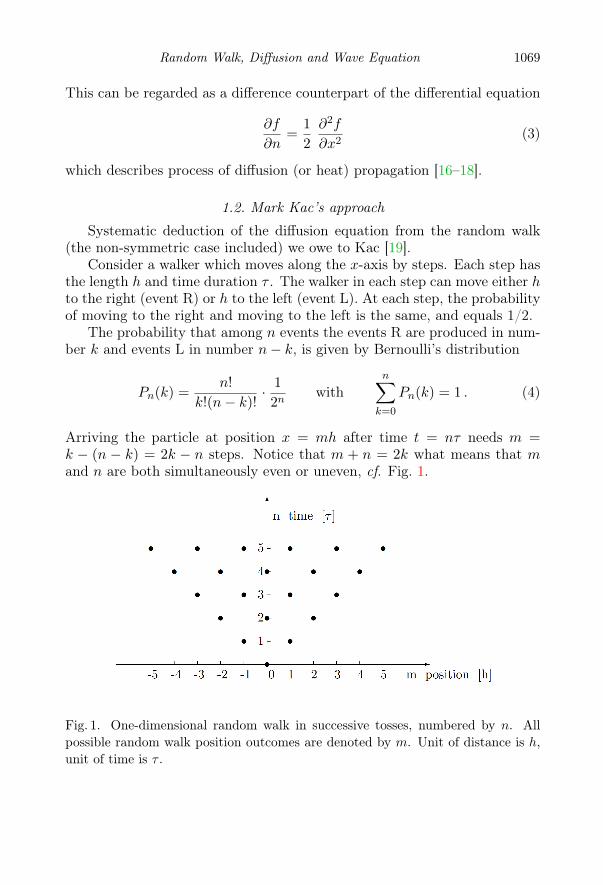
Arriving the particle at position x = mh after time t = nτ needs m =k − (n − k) = 2k − n steps. Notice that m + n = 2k what means that mand n are both simultaneously even or uneven, cf. Fig. 1.

Fig. 1. One-dimensional random walk in successive tosses, numbered by n. Allpossible random walk position outcomes are denoted by m. Unit of distance is h,unit of time is τ .

1070 R. Wojnar

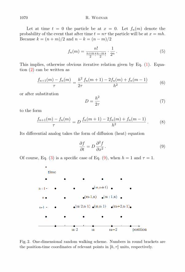
Let at time t = 0 the particle be at x = 0. Let fn(m) denote theprobability of the event that after time t = nτ the particle will be at x = mh.Because k = (n+m)/2 and n− k = (n−m)/2

fn(m) =n!

n+m2 !n−m2 !

· 12n. (5)

This implies, otherwise obvious iterative relation given by Eq. (1). Equa-tion (2) can be written as

fn+1(m)− fn(m)

τ=h2

2τ

fn(m+ 1)− 2fn(m) + fn(m− 1)

h2(6)

or after substitution

D =h2

2τ(7)

to the form

fn+1(m)− fn(m)

τ= D

fn(m+ 1)− 2fn(m) + fn(m− 1)

h2. (8)

Its differential analog takes the form of diffusion (heat) equation

∂f

∂t= D

∂2f

∂x2. (9)

Of course, Eq. (3) is a specific case of Eq. (9), when h = 1 and τ = 1.

Fig. 2. One-dimensional random walking scheme. Numbers in round brackets arethe position-time coordinates of relevant points in [h, τ ] units, respectively.

Random Walk, Diffusion and Wave Equation 1071

Be aware, however, that at the given time moment n, the distance be-tween neighbouring positions is 2h and that to the given position m, thewalker can return from neighbouring position after time 2τ . Thus, the point(m,n+1) is inaccessible for the walker being in (m,n) in the time period τ ,and in Eq. (2) or (8) the subtrahend function fn(m) is not determined, asthe point m,n is omitted in the random walk, cf. Fig. 2.

It is also important to notice that the diffusion Eq. (9) was obtained afterthe limits h→ 0 and τ → 0 were taken in such a way that the coefficient Dgiven by Eq. (7) was kept constant.

2. Random walk and wave equation

As the fn(m) appearing in (6) does not exist in a real random walkprocess, cf. Fig. 2, at the end of the previous section, we have indicated anapparent inconsistency of the Rayleigh–Kac scheme. It can be easily verifiedthat the realistic scheme reads

fn+1(m)− fn−1(m)

2τ=h2

2τ

fn−1(m+ 2)− 2fn−1(m) + fn−1(m− 2)

4h2(10)

and differs from Eqs. (2) or (8) by taking as the difference step for the spaceand time instead h and τ the quantities 2h and 2τ , respectively.

Indeed, the iteration (1) written in the form

fn+1(m) = 12 fn(m+ 1) + fn(m− 1)

implies analogical relations

fn(m+ 1) = 12 fn(m+ 2) + fn(m)

andfn(m− 1) = 1

2 fn−1(m) + fn−(m− 2)

what, after combination, gives

fn+1(m) = 14 fn−1(m+ 2) + 2fn−1(m) + fn−1(m− 2) . (11)

Hence, we get Eq. (10), which can be transformed into Fick’s diffusion equa-tion, after Rayleigh–Kac’s prescription.

However, this prescription is not a priori unique. Let us introduce thecontinuous function f(x, t) which in nodal points (mh, nτ), m, n — integer,takes values

f(x, t)(mh,nτ) = f(mh, nτ) = fn(m) .

1072 R. Wojnar

Applying Taylor’s expansion about the point (mh, (n − 1)τ) and keepingconsequently terms including the second order, we get the following approx-imation of the finite forward difference

fn+1(m)− fn−1(m) = 2τ∂f

∂t(mh, (n− 1)τ) + 1

2 (2τ)2 ∂

2f

∂t2(mh, (n− 1)τ) .

(12)In the similar manner, we get

fn−1(m+ 2) = fn−1(m) + 2h∂f

∂x(mh, (n− 1)τ) 1

2 (2h)2 ∂

2f

∂x2(mh, (n− 1)τ)

and

fn−1(m−2) = fn−1(m)−2h∂f

∂x(mh, (n− 1)τ)+ 1

2 (2h)2 ∂

2f

∂x2(mh, (n−1)τ) .

Addition of two least equations by sides and arranging of terms gives thefollowing expression for the second order central difference

fn−1(m− 2)− 2fn−1(m) + fn−1(m+ 2) = (2h)2∂2f

∂x2(mh, (n− 1)τ) . (13)

We substitute relations (12) and (13) into (10). Thus, by proceeding in thesimilar manner as it was done by Rayleigh and Kac, but keeping the secondderivatives in both, spatial and temporary variables, we get

τ∂2f

∂t2+∂f

∂t=h2

2τ

∂2f

∂x2(14)

or∂2f

∂t2+

1

τ

∂f

∂t= c2

∂2f

∂x2, (15)

where we have denoted

c2 =

(h

τ

)2

. (16)

Equation (15) has the form of wave equation of diffusion (or heat) propa-gating with the velocity c, discussed in [20–25]. We have also

τ =D

c2. (17)

In this derivation, the quantity τ is small but finite, and is known as therelaxation time for a phenomenon described by Eq. (15).

Notice also that, as a result of many-body stochastic interactions, thevelocity c is

√2 times smaller then the velocity of singular step equal to h/τ .

Analogical diminishing of velocity is presumed in three dimensions [25].The reason of obtaining different results (9) and (15) based on the same

difference algorithm (1) lies in admission of the second time derivative inthe substitution of finite difference equation by a differential one.

Random Walk, Diffusion and Wave Equation 1073

3. Wave equation of diffusion

Macroscopic derivation of the wave equation of diffusion is based on theassumption that the stream of the particles j is not generated by the den-sity gradient instantaneously (as in process described by the Fick’s diffusionequation), but it is delayed by a time τ0, called a relaxation time.

The continuity relation links temporal variation of the density of parti-cles f(x, t) with the spatial variation of the particle stream j, and in onedimension it reads

∂f

∂t= −∂j(x, t)

∂x, (18)

and if combined with Fick’s law of diffusion

j = −D ∂f

∂x, (19)

where D stands for the diffusion coefficient, the classical diffusion equa-tion (9) is obtained.

However, if there exists a certain time delay, τ0, between change of thedensity gradient and the stream generated by it

j(x, t+ τ0) = −D∂f

∂x

then, under assumption of a sufficiently small τ0, after expansion of theleft-hand side of the last equation into power series of τ0, one gets

j(x, t) + τ0∂j(x, t)

∂t= −D∂f

∂x. (20)

Hence, after applying the (one-dimensional) divergence operator

∂j(x, t)

∂x+ τ0

∂

∂t

∂j(x, t)

∂x= −D∂

2f

∂x2,

and after using the continuity equation (18), one obtains

τ0∂2f

∂t2+∂f

∂t= D

∂2f

∂x2(21)

what is known as the wave or hyperbolic diffusion equation, cf. Eq. (15), indistinction of the parabolic diffusion equation (9).

Equation (21) is the telegrapher’s type equation, cf. [26, 27]. It is worthto notice that such an equation was obtained also by Kac [24] after adopt-ing another scheme of interpretation of the non-symmetric random walk.Namely, Kac considered a particle starting from the original x = 0 and al-ways moving with the speed v. It can move either in positive direction or inthe negative direction. Each time the particle arrives at a lattice point, thereis a probability of reversal of direction. With these assumptions, Eqs. (15)or (21) can be obtained.

1074 R. Wojnar

4. Entropy of the system

To answer which way of interpretation of random walk, either this whichleads to parabolic diffusion or to hyperbolic one, the entropy growth of twoprocesses should be compared.

4.1. Entropy

Let as assume that the distribution density f is positive. After [28, 29],for the continuum limit of the Shannon entropy of our problem is accepted

S = −∫Ω

f(x, t) ln f(x, t)dx . (22)

Here, Ω denotes the infinite one-dimensional interval in which the diffusionis considered. We find by differentiation

dS

dt= −

∫Ω

∂f(x, t)

∂tln f(x, t)dx−

∫Ω

∂f(x, t)

∂tdx , (23)

or after using the continuity relation (18)

dS

dt=

∫Ω

ln f(x, t)∂j(x, t)

∂xdx+

∫Ω

∂j(x, t)

∂xdx . (24)

By the (one-dimensional) divergence theorem, the second term at right-handside is zero, if there are no particle flows at infinity, and

dS

dt= −

∫Ω

ln f(x, t)∂j(x, t)

∂xdx .

Once again, the integration by parts gives

dS

dt=

∫Ω

1

f(x, t)

∂f(x, t)

∂xj(x, t)dx

ordS

dt=

∫Ω

1

f(x, t)

1

D

j(x, t) + τ0

∂j(x, t)

∂t

j(x, t)dx , (25)

where the relation (20) was exploited.

Random Walk, Diffusion and Wave Equation 1075

4.2. Entropy growth

The last result can be written as

dS

dt= J2 +

1

2τ0dJ2

dt, (26)

whereJ2 ≡

∫Ω

1

f(x, t)Dj(x, t)2dx . (27)

In the limiting case, when the entropy production rate vanishes (dS/dt = 0),we get by Eq. (26)

J2 = J20 e−2t/τ0 . (28)

On the other hand, for τ0 = 0, the entropy production rate according toEq. (26) is always non-negative. For τ0 6= 0, by integration of Eq. (26), wefind

J2 − J20 e−2t/τ0 =

2t

τ0e−2t/τ0

t∫0

dS

dt′e2t′/τ0dt′ . (29)

IfJ2 > J2

0 e−2t/τ0 , (30)

then also dS/dt > 0.In general, however, the criterion (26) is too weak to judge whether

the process is thermodynamically consistent [28]. One can argue that forsufficiently small τ0, this inequality may be satisfied, and the wave equationof diffusion seems to be affirmed in some experiments [30, 31].

4.3. Density distribution

Mathematical form of Eq. (21) is identical with the telegrapher’s equa-tion, which describes the voltage or current on an electrical transmission linewith distance and time [26, 27]. Its Green’s function reads

f(x, t) = 2π c e− t

2τ0J0(

1

2√Dτ0

√x2 − c2t2

)η(ct− x) , (31)

wherec2 ≡ D

τ0

denotes square of the velocity of diffusive wave and η(x) is the unit stepfunction (equal 1 for x non-negative, and zero for x negative).

1076 R. Wojnar

This solution achieves non-zero values for finite x only, x ≤ ct, but, inspite of the definition of probability, it admits also the negative values dueto the properties of Bessel function J0, and for this reason it cannot beadequate for the problem of diffusion.

For the same reason, one cannot look for the solution of Eq. (21) in formof a damped wave

f = f0 ei(kx−ωt)

which is typical to the telegrapher’s equation.

5. Fick’s diffusion

Green’s function for the one-dimensional diffusion equation (9) reads

f(x, t) =1

2√πDt

e−x2

4Dt . (32)

From this formula, we deduce that if in a region whose dimension is of theorder of length `, a non-uniform distribution is introduced, the order of mag-nitude tR of the time required for the distribution to become approximatelythe same throughout the region is

tR ≈`2

D. (33)

The time tR may be called the relaxation time for the density equalisationprocess [17].

The diffusion process described by formula (32) has the property thatfor any t > 0, the function f(x, t) > 0 in the whole space, it is the effectof the initial perturbation, is propagated instantaneously through all space.Some authors interpret this property as an admission of the infinite speed ofmass distribution and hence, the violation of the rules of physics. To avoidsuch contradiction, called a paradox, they use a hyperbolic diffusion equa-tion (15), instead of the parabolic (9). For example, they use the hyperbolicdiffusion equation to study the transport process of electrolytes in mediasuch as gels and porous media [30, 31].

However, the paradox is only apparent and does not object to the phys-ical reality. The mass of substance which is to be found at time t furtherfrom the source, then a is

∞∫a

f(x, t)dx =

∞∫a

1

2√πDt

e−x2

4Dtdx (34)

and as a→∞, it becomes negligibly small.

Random Walk, Diffusion and Wave Equation 1077

6. Arising of the paradox

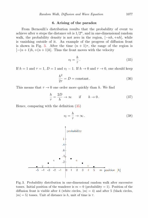
From Bernoulli’s distribution results that the probability of event toachieve after n steps the distance nh is 1/2n, and in one-dimensional randomwalk, the probability density is not zero in the region, [−nh,+nh], whileis vanishing outside of it. An example of the progress of diffusion frontis shown in Fig. 3. After the time (n + 1)τ , the range of the region is[−(n+ 1)h,+(n+ 1)h]. Thus the front moves with the velocity

vf =h

τ. (35)

If h = 1 and τ = 1, D = 1 and vf = 1. If h→ 0 and τ → 0, one should keep

h2

2τ= D = constant . (36)

This means that τ → 0 one order more quickly than h. We find

h

τ=

2D

h→∞ if h→ 0 . (37)

Hence, comparing with the definition (35)

vf =h

τ→∞ . (38)

Fig. 3. Probability distribution in one-dimensional random walk after successivetosses. Initial position of the wanderer is m = 0 (probability = 1). Position of thediffusion front is visible after 4 (white circles, |m| = 4) and after 5 (black circles,|m| = 5) tosses. Unit of distance is h, unit of time is τ .

1078 R. Wojnar

The range of the distribution after n steps is r = nh, and the time necessaryto build up such range is t = nτ . The height of the diffusion front diminishes,however, with n as 1/2n. Hence

n =t

τand r = nh =

t

τh = t vf .

For any finite time t, in the limit of τ → 0 and h → 0, the range r → ∞,because of (38), the height of the front reduces to zero, and the paradox ofinstantaneous propagation without front arises.

7. The diffusion coefficient

The diffusion coefficient (7) for the symmetric random walk

D =h2

2τ(39)

is similar to that given by the kinetic theory of gases [32]

D = 12 h

h

τ. (40)

It reveals also an analogy with Einstein’s relation [4, 5]

D =

⟨x2⟩

2t, (41)

where 〈x2〉 is an average squared deviation of a distinct particle in the Brow-nian movement realised in the time t.

From Eq. (33), we obtain

D ≈ `2

tR. (42)

It is worth mentioning that the last relation obtained from the macroscopictheory has a similar form to relations (39)–(41), obtained from the micro-scopical theories. This persistence of the form argues also for the parabolicinterpretation of the random walk.

8. Non-symmetric random walk

In this case, at each step, the probability of moving to the right (event R)is p and moving to the left (event L) is q = 1−p. In symmetrical Rayleigh’scase p = q = 1/2, while the general non-symmetric case of p 6= q was treatedby Kac [19].

Random Walk, Diffusion and Wave Equation 1079

The probability that among n events the events R are produced in num-ber k and events L in number n− k is given by Bernoulli’s distribution

Pn(k) =n!

k!(n− k)!pk(1− p)n−k with

n∑k=0

Pn(k) = 1 . (43)

As in the symmetrical case, finding the particle at position x = mh aftertime t = nτ needs m = k − (n− k) = 2k − n steps, cf. Fig. 1.

Let at time t = 0 the particle be at x = 0. Then,

fn(m) =n!

n+m2 !n−m2 !

pn+m

2 (1− p)n−m

2 (44)

denotes the probability of the event that after time t = nτ the particle willbe at x = mh. This implies, otherwise obvious iterative relation

fn+1(m) = (1− p)fn(m+ 1) + pfn(m− 1) (45)

instead of relation (1).A positive quantity ε may be defined such that

p ≡ 12 + ε and 1− p = 1

2 − ε . (46)

Then, Eq. (45) may be written as

fn+1(m) =(12 − ε

)fn(m+ 1) +

(12 + ε

)fn(m− 1) . (47)

For ε = 0, we get Rayleigh’s case (1).In a similar manner as Eq. (45), two other iterative relations can be

written

fn(m− 1) =(12 + ε

)fn−1(m− 2) +

(12 − ε

)fn−1(m) , (48)

andfn(m+ 1) =

(12 + ε

)fn−1(m) +

(12 − ε

)fn−1(m+ 2) . (49)

Substituting (48) and (49) into (45), we get

fn+1(m) = 14 [fn−1(m− 2) + 2fn−1(m) + fn−1(m+ 2)]

+ ε [fn−1(m− 2)− fn−1(m+ 2)]

+ ε2 [fn−1(m− 2)− 2fn−1(m) + fn−1(m+ 2)] . (50)

Similarly, as in the symmetrical case, at the given time n, the distancebetween neighbouring positions is 2h and that the return to the given posi-tion m is possible after the time period 2τ , only, cf. Fig. 2.

1080 R. Wojnar

9. Difference equation of diffusion with drift

We subtract from both sides of (50) the quantity fn−1(m)

fn+1(m)−fn−1(m) =(14 + ε2

)[fn−1(m− 2)− 2fn−1(m) + fn−1(m+ 2)]

+ ε [fn−1(m− 2)− fn−1(m+ 2)] , (51)

and transform it as follows

fn+1(m)− fn−1(m)

2τ

=(14 + ε2

) (2h)2

2τ

fn−1(m− 2)− 2fn−1(m) + fn−1(m+ 2)

(2h)2

+ ε4h

2τ

fn−1(m− 2)− fn−1(m+ 2)

4h. (52)

After introducing the notation

D =(1 + 4ε2

) h22τ

andD

T

∂V

∂x=

2h

τε , (53)

we get

fn+1(m)− fn−1(m)

2τ= D

fn−1(m− 2)− 2fn−1(m) + fn−1(m+ 2)

(2h)2

+D

T

∂V

∂x

fn−1(m− 2)− fn−1(m+ 2)

4h. (54)

This can be regarded as a difference counterpart of the differential equa-tion of Smoluchowski’s diffusion, known also as the diffusion equation withdrift [6, 7]. The exterior force (− ∂V/∂x) is the cause of the drift. Thequantity T is the temperature in units of the energy. Here, in contrast toKac’ results [19], the diffusion coefficient D is modified by the non-symmetryindicator ε.

10. Differential equation of diffusion and wave equation

Despite of formal similitude of equations (52) and (10), the transitionh → 0 and τ → 0, necessary to obtain differential equation of diffusion,is in the case of Eq. (52) more difficult. Namely, because according toequation (53)

D ∝ h2

τwhile

D

T

∂V

∂x∝ h

τ, (55)

Random Walk, Diffusion and Wave Equation 1081

it is impossible to keep simultaneously the diffusion coefficient

D ∝ h2

τ= constant , (56)

and the drift force

− ∂V∂x∝ 1

h

h2

τ(57)

non-singular. To avoid this singularity, Kac proposed to use the substitu-tion [19]

ε = βh with β = constant (58)

which assures the non-singularity of the drift force. But this means, whenh → 0, then also ε → 0 and only the very small deviations from symmetryof the random walk, and consequently very small drift forces in Eq. (54) arepermitted.

However, if instead of (56) and (57), we accept the following limit rela-tions for h→ 0 and τ → 0

h

τ∝ v = constant , (59)

thenh2

τ∝ D → 0 , (60)

and Eq. (54) becomes

fn+1(m)− fn−1(m)

2τ= v

fn−1(m− 2)− fn−1(m+ 2)

4h(61)

withv = ε

4h

2τ. (62)

After passing to limit with h and τ , we get

∂f

∂t= − v ∂f

∂x. (63)

It is, the so-called advection equation, closely related to the wave equation.The constant v is the speed of wave motion.

11. Conclusions

The description of diffusion as a random walking resembles the hoppingmodels proposed in [33], and by Grasselli and Streater [34].

1082 R. Wojnar

Notice also that for the non-symmetric walk when ε 6= 0, not only thedrift force, but also the diffusion coefficient depends on ε. This is conformto the phenomenological description of the two-level diffusion, where thechange of the potential for external drift force is accompanied by the changeof diffusion coefficient [28].

Random walk is a certain mathematical tool, characterised by the iter-ative relation (1) for the symmetric coin, and relation (45) for the non-symmetric one. As every mathematical concept, it receives its physicalmeaning after appropriate attribution of physical quantities to the mathe-matical terms. In our case, the appropriateness denotes the agreement withthe laws of thermodynamics, and we must chose between different proposalsof interpretation.

It is widely accepted that the random walk is a simplified picture ofdiffusion phenomena the most famous example of which is the Brownianmovement. However, another hyperbolic interpretations of the random walkare possible.

If one assumes the fraction h2/(2τ) to be constant when the limits h→ 0and τ → 0 are taken, then Fick’s diffusion equation is obtained, while as-sumption that the quotient h/τ keeps constant leads to the wave diffusionequation. It seems interesting that the same pattern appears at differentlevels of the diffusion analysis. This is a strong support for the classical(parabolic) interpretation of the random walk, cf. Section 7.

We indicated the controversies to which the hyperbolic equation of diffu-sion is leading, especially the possibility of appearing of non-positive densityand decreasing entropy. The inconvenience of the classical diffusion man-ifested in the so-called infinite speed paradox seems to be unimportant incomparison. The infinite range of the classical distribution, for any timet > 0, appears as a mathematical effect, in result of limit passage to in-finitesimal increments, and corresponds to Einstein’s formula for Browniandiffusion.

Between several possible interpretation of the random walk mathematicalprocess, one should choose those which are conform to the physical rules. Inour case, this role of Occam’s razor is realised by two laws: the positivity ofthe probability density, and the entropy growth of free system.

REFERENCES

[1] K. Pearson, The Problem of the Random Walk, Nature 72, 294 (1905).[2] J.W. Strutt, Lord Rayleigh On the Resultant of a Large Number of

Vibrations of the Same Pitch and of Arbitrary Phase, Philos. Mag. 10, 73(1880).

Random Walk, Diffusion and Wave Equation 1083

[3] J.W. Strutt, Lord Rayleigh, The Theory of Sound, Volume 1, section 42a,Second edition revised and enlarged, Dover Publications, New York 1945.

[4] A. Einstein, Über die von der molekularkinetischen Theorie der Wärmegeforderte Bewegung von in ruhenden Flüssigkeiten suspendierten Teilchen,Ann. Phys. 322, 549 (1905).

[5] A. Einstein, Über die von der molekularkinetischen Theorie der Wärmegeforderte Bewegung von in ruhenden Flüssigkeiten suspendierten Teilchen,J. Barth, Leipzig 1905.

[6] M. v. Smoluchowski, Drei Vortäräge über Diffusion, BrownscheMolekularbewegung und Koagulation von Kolloidteilchen, PhysikalischeZeitschrift 17, 557 (1916); 17, 587 (1916).

[7] S. Chandrasekhar, M. Kac, R. Smoluchowski, Marian Smoluchowski — HisLife and Scientific Work, ed. R.S. Ingarden, PWN, Warszawa 1999.

[8] N.W. Goel, N. Richter-Dyn, Stochastic Models in Biology, Academic Press,New York 1974.

[9] P.G. De Gennes, Scaling Concepts in Polymer Physics, Cornell UniversityPress, Ithaca, London 1979.

[10] M. Doi, S.F. Edwards, The Theory of Polymer Dynamics, Clarendon Press,Oxford 1986.

[11] N.G. Van Kampen, Stochastic Processes in Physics and Chemistry, revisedand enlarged edition, North-Holland, Amsterdam 1992.

[12] S. Redner, A Guide to First-passage Process, Cambridge University Press,Cambridge, UK 2001.

[13] H. Kleinert, Path Integrals in Quantum Mechanics, Statistics, PolymerPhysics, and Financial Markets, 4th edition, World Scientific, Singapore2004.

[14] R. Wojnar, Acta Phys. Pol. A 114, 607 (2008).[15] R. Wojnar, Acta Phys. Pol. A 123, 624 (2013).[16] H.S. Carslaw, J.C. Jaeger, Conduction of Heat in Solids, Clarendon Press,

Oxford 1948.[17] L.D. Landau, E.M. Lifshitz, Fluid Mechanics, Vol. 6 of Course of Theoretical

Physics, 2nd English ed., translated from Russian by J.B. Sykes, W.H. Reid,Pergamon Press, Oxford–New York–Beijing–Frankfurt–Sao Paulo–Sydney–Tokyo–Toronto 1987.

[18] R. De Groot, P. Mazur, Non-Equilibrium Thermodynamics, North-HollandPubl. Co, Amsterdam 1962.

[19] M. Kac, Am. Math. Mon. 54, 369 (1947).[20] C. Maxwell, On the Dynamical Theory of Gases, Philos. Trans. R. Soc.

London 157, 49 (1867).[21] C.R. Cattaneo, Sulla conduzione del calore, Atti Sem. Mat. Fis. Univ.

Modena 3, 83 (1948).

1084 R. Wojnar

[22] C.R. Cattaneo, Sur une forme de l’équation de la chaleur éliminant leparadoxe d’une propagation instantanée, Comptes Rendus Acad. Sci. 247,431 (1958).

[23] P. Vernotte, Les paradoxes de la theorie continue de l’équation de la chaleur,Comptes Rendus Acad. Sci 246, 3154 (1958).

[24] M. Kac, Rocky Mountain J. Math. 4, 497 (1974).[25] M. Chester, Phys. Rev. 131, 2013 (1963).[26] Ph.M. Morse, H. Feshbach, Methods of Theoretical Physics, McGraw-Hill,

New York–Toronto–London 1953, Section 7.4.[27] M. Suffczyński, Elektrodynamika, PWN, Warszawa 1964, in Polish.[28] R.F. Streater, Rep. Math. Phys. 40, 557 (1997).[29] Z. Burda, J. Duda, J.M. Luck, B. Waclaw, Phys. Rev. Lett. 102, 160602

(2009).[30] J.R. Ramos-Barrado, P. Galan-Montenegro, C. Criado Combon, J. Chem.

Phys. 105, 2813 (1996).[31] C. Criado, P. Galan-Montenegro, P. Velasquez, J.R. Ramos-Barrado,

J. Electroanal. Chem. 488, 59 (2000).[32] O.E. Meyer, De gasorum theoria, Dissertatio inauguralis

mathematica–physica, Maelzer, Vratislaviae 1866.[33] R.F. Streater, Proc. Roy. Soc. A456, 205 (2000).[34] M.R. Grasselli, R.F. Streater, Rep. Math. Phys. 50, 13 (2002).