The habit for voting, “civic duty” and travel distance

Tim Pawlowski and Dennis Coates

Tim Pawlowski

Faculty of Economics and Social Science, Institute of Sports Science

University of Tübingen

Wilhelmstraße 124

72074 Tübingen, Germany

Phone: +49(0)7071-29-76544

FAX: +49(0)-7071-29-5031

Email: tim.pawlowski@uni-tuebingen.de

Dennis Coates

Department of Economics,

University of Maryland Baltimore County

1000 Hilltop Circle, Baltimore, MD 21250

Phone: 410-455-2160

FAX: 410-455-1054

Email: coates@umbc.edu

Keywords: voting participation; election turnout; travel distance; travel cost

Abstract: There is a rich literature addressing the paradox of not voting and

election turnout from both theoretical and empirical perspectives. By taking

advantage of a unique dataset from an “experimental” setting, this paper is the

first to estimate the utility that drives the “civic duty” or the habit for voting.

Consistent with the general turnout literature, education level, marital status,

household size, and distance all affect the persistence of voter participation.

2

1. Introduction

An enormous literature addresses the paradox of not voting and election

turnout from both theoretical and empirical perspectives (Downs, 1957; Tullock,

1967; Riker and Ordeshook, 1968; Wolfinger and Rosenstone, 1980; Powell,

1986; Ledyard, 1981, 1984; Palfrey and Rosenthal, 1983, 1985; Cox and Munger,

1989; Matsusaka and Palda, 1993; Knack, 1994; Fort, 1995; Morton, 1991;

Shachar and Nalebuff, 1999; Green and Sachar, 2000; Feddersen and Sandroni,

2006; Coate and Conlin, 2004). The literature is vast because the Downsian

(1957) model of the rational voter raises an interesting puzzle: individual voters

have expected benefit of zero from voting, because each has an infinitesimally

small chance of affecting the outcome of the vote, while voters incur positive

costs of voting, for a negative expected net benefit of voting, yet many people

vote.

The first explanation for this paradox proposed that people voted out of a

sense of civic duty. This apparent deus ex machina asserts that people derive a

consumption benefit from the act of voting which is sufficiently large to

overcome the costs of voting, at least for some voters. Moreover, the size of this

consumption benefit can vary from issue to issue, and may be affected by the

efforts of other individuals or groups, such as campaign spending and get out the

vote drives.

The second explanation for the paradox suggested that the probability of

affecting the outcome may not be infinitesimal after all. If one believes that all

other voters will not vote, because they feel they cannot alter the outcome, then no

one votes, and one voter who decides to vote will in fact be certain to affect the

outcome. Game theoretic models building on this insight find there will be turnout

to vote in equilibrium, even without reliance on a consumption benefit from

voting.

3

In this paper we take advantage of a unique dataset to both estimate and

control for the impact of “civic duty” or the inherent consumption benefit in a

model that estimates the impact of travel cost on the persistence in voter

participation, i.e. the habit for voting. Our setting is attendance at the annual

meeting of the membership of one of the biggest professional football clubs in

Germany, with more than 71,000 club members. At the annual meetings, club

members in attendance vote on club leadership positions and policies. For

instance, each third year one of the four directors of the club is elected using

simple majority rule.

While the issues under consideration by the football club are different

from those in an election for a governmental position or policy, concerns about

participation, or turnout, related to costs and benefits of voting are similar.

Consequently, we argue that general conclusions about voting participation

behavior can be drawn from our setting. Moreover, our unique dataset affords us

the opportunity to address “civic duty” and consumption benefits of voting in a

novel way.

Club members were surveyed about their voting behavior, reasons for

attending or not attending the annual meetings, attendance at club football

matches, and participation in other social and political organizations. Attendance

at the annual meetings is a requirement for voting, and survey respondents

indicated their frequency of attending as never, seldom, sometimes, or often. Our

dependent variable indicates the persistence in voter participation, letting us

estimate ordered probit models of voter participation, with a focus on a habit for

voting.

The hurdle parameters of the ordered probit model provide estimates of

the impact of the feelings of civic duty on the decision to participate. Moreover,

using estimates of the impact of travel distance we are able to assess the

sensitivity of habitual voter participation to changes in travel cost and other

4

factors. Our results indicate that distance matters for voting, as do setting-specific

variables like length of club membership and whether or not the individual

belongs to more than one sport club. Consistent with the general turnout literature,

education level, marital status and household size also affect participation.

The next section of the paper, section 2, is a brief review of the voter

participation literature. Our purpose in this section is to describe the state of the

literature and to make clear how our analysis contributes to an understanding of

voter participation. In section 3 we describe the data, and the survey from which it

is derived. Section 4 develops the empirical model of persistent or habitual voter

participation. Section 5 presents the estimation results and evaluation of the

impact of distance on the persistence of voting. Section 6 concludes.

2. Literature

In the early literature on voter turnout (Tullock, 1967; Riker and

Ordeshook, 1968) the decision to vote is often discussed with respect to a

comparison of the cost of voting with the expected benefits of voting. Given that

the likelihood that an individual voter’s ballot alters the outcome of the election is

vanishingly small, the decision calculus can only lead to voting if there are

benefits from participation that are independent of the outcome of the election.

The expected benefits from the policy outcome are called instrumental

benefits. The benefits from participation are sometimes described as arising from

doing one’s “civic duty”, for example, but they are also explained as voting for

reasons other than concern for the actual outcome of the election. For instance,

the decision to vote may be motivated by benefits derived directly from the act of

voting. A voter may also derive benefits from voting for or against a particular

alternative independent of the outcome of the election. For example, one might

vote in support of the environment or in opposition to gay marriage not because of

one’s expected net benefits from the favored outcome, but rather because one is

5

expressing support for a moral or ethical position. Voting motivated in this

“public minded” way is called expressive voting. Whether voting is explained as

instrumental or expressive, or because people vote because they feel it is their

civic duty or because they derive happiness from participation, these explanations

focus on the individual voter first.

Ledyard (1981, 1984) and Palfrey and Rosenthal, (1983, 1985) developed

game-theoretic models in which the probability of being the decisive voter is

endogenous. These models do not require a consumption benefit from voting to

generate positive turnout. More recently, scholars have sought explanations for

individual participation in voting using the behavior of groups (Morton, 1991;

Shachar and Nalebuff, 1999; Feddersen and Sandroni, 2006; Coate and Conlin,

2004). While the individual voter still decides whether or not to vote, the

motivation to vote is influenced by the activities of groups. These models rely on

the existence of consumption benefits from voting and focus on explaining

changes in those benefits to explain the paradox of nonvoting (Feddersen, 2004).

For example, political parties, party leaders, or other interested organizations

might engage in voter mobilization drives (Pollock, 1982; Morton, 1991; Shachar

and Nalebuff, 1999). Alternatively, voter participation may derive from a set of

ethical norms to act in the best interests of the group to which the voter belongs

(Feddersen and Sandroni, 2006; Coate and Conlin, 2004). These ethical voters

consider different behavioral rules, comparing them according to their results

when everyone in their group acts according to the same rule. In addition, ethical

voters derive satisfaction from following the rule that they determine produces the

best group outcome from among the various possible rules.

Finally, there is evidence that voters may develop a habit for voting. That

is, people who have voted in the past are significantly more likely to vote again.

Green and Shachar (2000) use panels from the American National Election Study

to examine voting behavior in successive elections. Their intent is to avoid

6

problems of unobserved heterogeneity and bias using recursive regression and

instrumental variables to control for personal and situational determinants of

voting that may persist over time. They find a significant impact of voting

previously on the probability of voting in the current election. Gerber, Green, and

Shachar (2008) extend the analysis using an experimental design in which some

voters are encouraged to vote in a specific election and others are not. Those that

were encouraged to vote were more likely to do so both in the first election and in

a subsequent election a year later. They conclude that the increase is the result of

voting becoming a habit, supposing that unobservable heterogeneity has remained

constant from election to election. Of course, whether unobservable heterogeneity

is in fact constant is unknown and unknowable, but one could also infer that the

treatment, that is, the encouragement to vote, changes the unobservable

heterogeneity in favor of voting for those voters who get the treatment. In other

words, the treatment introduced by Gerber, Green, and Shachar (2008) enhances

the consumption benefits from voting, and this enhancement is persistent.

Regardless of the source of these consumption benefits, the decision to

vote will also depend on the cost of voting. Costs of voting include such things as

educating oneself on the issues, the time spent waiting to enter the voting booth,

and the costs of transportation to the polling station. The higher are the costs of

voting, the fewer the voters for whom the consumption benefits of voting exceed

the costs of voting, and the lower will be the turnout (see Matsusaka and Palda,

1993; Knack, 1994; Gibson, J., Kim, B., Stillman, S. & Boe-Gibson, 2012;

Haspel, M. & Knotts, H. G., 2005).

Munger (2001) conceptualizes the total vote on a ballot measure as a share

of the population as the product of four ratios, the share of the population that is

enfranchised, the share of those that are enfranchised that are also registered, the

share of those that are registered that enter the voting booth, and the share of those

that enter the booth that vote on the specific ballot measure. The literature on

7

turnout focuses on the last two of these ratios, and generally assumes that there is

only one item on the ballot so that everyone who enters the booth in fact votes.1 In

other words, much of the literature throws away useful information about turnout

by focusing on a single election. Cox and Munger (1989) relax this assumption by

accounting for presidential and senatorial campaign spending when evaluating the

impact of spending by candidates for the House of Representatives. Nownes

(1992), Green and Shachar (2000) and Gerber, Green, and Shachar (2008) relax it

further by considering participation in multiple elections by the same voters.

Nownes (1992), who estimates a multinomial logit model in which those eligible

to vote may turn out to neither the primary nor the general election, may turn out

only in the general election, or turn out to both, is most like what we do here.

Indeed, his discussion of the three categories of voters is highly suggestive of our

approach, that the voter interest is ordered from least to most interested in politics.

Our approach is also consistent with the findings by Fowler, Baker and

Dawes (2008), Fowler and Dawes (2008) and Loewen and Dawes (2012) that a

proclivity for voting is connected to genetics. By using all turnouts by our voters

to construct an indicator of the strength of the urge to vote, our analysis is able to

shed light on the impact that other factors may have in mitigating the urge. For

example, Fowler and Dawes (2008) find that the impact of having the genetic

marker that leads to a greater likelihood of voting is larger for those that attend

religious services. They also find that higher income, greater cognitive abilities,

more partisanship, and college education enhance the likelihood of voting. But

their regressions do not contain any measure of the cost of voting, such as

distance from the polling place.

1 Fort (1995) estimates a recursive model of voting on a specific issue in which the first step is to

explain registration, then turning out to the polls, and finally voting once in the booth.

8

3. Data

We take advantage of a unique dataset to analyze the role of “civic duty”

in a model that estimates the impact of travel cost on the decision to vote. Our

analysis is not of a typical political environment of a national, regional or local

election. Rather our “experimental” setting is attendance at the annual meeting of

the membership of one of the biggest professional football clubs in the first

division of the German Bundesliga, i.e. the club Hamburg Sport-Verein (HSV).2

At the annual meetings, club members in attendance vote on various issues related

to the club’s policies. For instance, each third year they vote directly on one of the

four directors of the club via simple majority voting. Every year, voting occurs on

issues concerning club governance, amending bylaws, and so on.

Overall, the club has more than 71,000 members. At the date of inquiry

57,612 members were at least 16 years old and therefore (in general) eligible to

vote. However, in contrast to the ever increasing membership figures (starting

from around 7,000 in 1996), the number of members making use of their voting

right remains rather small. For instance, only around 2% of all members eligible

to vote attended the annual assembly on 15 January 2012 where Oliver Scheel

was re-elected as the fourth director of the club. Since issues related to costs and

benefits of voting as well as the overall participation decision are relevant to

voting in this case just as they are in voting participation decisions in general

(political) elections, we contend that conclusions based on an in-depth analysis of

our “experimental” setting can be extended to the general election context.

Our dataset is based on an online survey of the club members. Between 23

July and 5 August 2012 all members eligible to vote were surveyed about their

voting behavior and other related issues. The final adjusted net sample of

2 HSV offers competition and training in 30 sports and is the only club to have been in the top

division every year since the formation of the league in 1963. Club members get voice and vote, as

well as season tickets to the football matches at member prices, priority access to tickets for top

home and away matches, and discounted travel packages to away matches.

9

respondents (n=9,090) consists of 15.8% of the voting-eligible population and is

representative with regard to the geographic distribution of the club members as

well as their age and gender (see Figures 1 and 2).

The variables in the analysis are defined in Table 1. The dependent

variable is attendance at the football club’s annual meetings (with possible

answers of never, seldom, sometimes, and often). We equate attendance at the

annual meeting with voting, and frequency of attendance with frequency of

voting. At first sight, this may seem a problematic assumption as attending the

meetings may occur for a variety of reasons. However, the survey also asks

members who have attended the meetings sometimes or often about their

motivation for doing so (see Figure 3). Here, voting appears to be by far the

strongest motivation for attendance with about 95% of respondents who strongly

agree or tend to agree with the statement that they attend the meetings

predominantly to vote. On these grounds, we feel equating attendance with voting

is justifiable.

The choice of explanatory variables in the analysis is guided by the

existing voter turnout literature. Consequently, we include the voter’s age and age

squared, educational level, family size, marital status, income, and distance from

the voting location. The distance variable is measured as the travel distance by car

between the center of the 2-digit zip-code of residence and that of the venue of the

assembly in Hamburg (in kilometers). Our variables also include responses to four

questions about the voter’s other activities. Voters respond to questions about

their frequency of activity in four categories, sport participation, volunteer work,

political participation, and religious activities. Responses range from never

participate to weekly participation. Since the level of participation in these

activities is a choice, just like the decision to attend the annual club meetings to

vote, we are concerned that these variables are likely to be correlated with the

10

unobservable error in the regression model. Therefore, while we estimate the

model including these variables, our preferred model omits them.

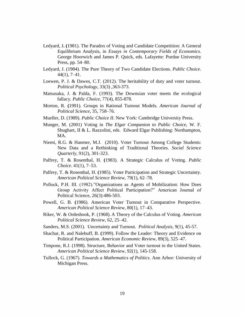
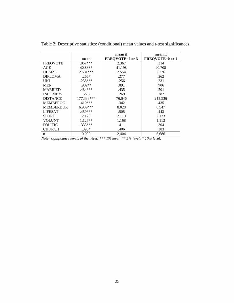
In Table 2, the mean values of each of the variables is reported for the full

sample in the regression and split into the least frequent and most frequent voters.

The asterisks indicate the level of statistical significance for rejection of the null

hypothesis that the split sample means are equal. Those club members that vote

most regularly are slightly older, better educated, live in smaller households, are

somewhat more likely to be female, and unmarried than are the less frequent

voters. More frequent voters are also less likely to belong to another sports club,

to have been members of HSV longer, and to feel more strongly that success of

the club affects their satisfaction with life. More frequent voters are also more

frequently involved in volunteer work and in political parties. There is no

statistical difference between the more frequent voters and less frequent voters

regarding sports participation or religious activities. Finally, more frequent voters

live substantially closer to the assembly meeting place than do the less frequent

voters.

4. Modeling persistent voting behavior

Club members’ voting behavior is assumed to derive from their utility

maximization. Unlike the typical model where the decision to vote focuses on one

specific election the focus here is put on the pattern of participation in multiple

elections over time, i.e. a habit for voting. We begin by assuming that for each

club member there is an unobserved utility of voting Ui that depends upon the

instrumental, expressive, and any consumption benefits and costs. These benefits

and costs are represented by vector Xi and the marginal influence of these benefits

and costs is reflected in the parameter vector β. The error term or random element

εi captures unobserved and unobservable influences on voting behavior, including

the benefits from doing one’s duty, from the act of participation, or genetic

11

predisposition. In other words, large values of εi will be associated with more

frequent voter participation, all other things constant; small values of εi will be

associated with less frequent voting. The utility function is

𝑈𝑖 = 𝑋𝑖𝛽 + 𝜀𝑖 (1)

To estimate the parameter vector β we utilize the club member’s reported

frequency of participation in voting, 𝑈𝑖𝑂. 𝑈𝑖

𝑂 = 0, 1, 2, 3, where 0 indicates the

member never votes, 1 indicates the member seldom votes, 2 that the member

sometimes votes, and 3 that the member often votes, as reported in the survey of

club members. We link the reported participation with the utility function as

follows

𝑈𝑖𝑂 = 0 𝑖𝑓 𝑈𝑖 = 𝑋𝑖𝛽 + 𝜀𝑖 ≤ 𝜇1 (2)

That is, the club member reports never voting if 𝜀𝑖 ≤ 𝜇1 − 𝑋𝑖𝛽, where μ1 is a

threshold parameter to be estimated. Similarly, a voter reports seldom voting if

𝑈𝑖𝑂 = 1 𝑖𝑓 𝜇1 < 𝑈𝑖 ≤ 𝜇2 or 𝜇1 − 𝑋𝑖𝛽 < 𝜀𝑖 ≤ 𝜇2 − 𝑋𝑖𝛽 (3)

where μ2 is a second threshold parameter to be estimated. The voter that reports

voting sometimes satisfies the following

𝑈𝑖𝑂 = 2 𝑖𝑓 𝜇2 < 𝑈𝑖 ≤ 𝜇3 or 𝜇2 − 𝑋𝑖𝛽 < 𝜀𝑖 ≤ 𝜇3 − 𝑋𝑖𝛽 (4)

and the voter that reports voting often satisfies

𝑈𝑖𝑂 = 3 𝑖𝑓 𝑈𝑖 = 𝑋𝑖𝛽 + 𝜀𝑖 > 𝜇3 or 𝜀𝑖 > 𝜇3 − 𝑋𝑖𝛽 (5)

This model is an ordered probit, with the three threshold parameters dividing the

voters according to the degree to which their voting is based on “civic duty”,

enjoyment from participation in club governance, or genetics.

12

The vector of explanatory variables Xi includes the variables described in

Table 1 under socio-demographic characteristics, member characteristics, and

leisure time engagement.

Voter age (AGE) entered quadratically, allowing the marginal impact to

rise or fall as one ages, reach a maximum or minimum, and then fall or rise. A

consistent finding in the voting literature is that older citizens are more likely to

vote than younger individuals, so we expect this to be true in our data as well.

Furthermore, our expectation on greater household size (HHSIZE) is that it will

be negative, reflecting likely greater opportunity cost of attending the annual

meetings (which might easily last 6 hours). In addition, we expect that regular

voting is more likely for male voters (MEN), for married voters (MARRIED), and

for voters with greater education (DIPLOMA and UNI). DIPLOMA indicates a

lower level of education than UNI, the omitted category is the least amount of

education, and it is possible that these two levels of education have different

effects on likely voting participation. Nonetheless, we expect both coefficients to

be positive. We had no expectation about the impact of income on the proclivity

to vote. In the literature, justifications for the inclusion of income include that

income measures a voter’s stake in the outcome, is a proxy for political interest or

awareness of the issues, measures productivity in political activity (Frey, 1971),

or represents the opportunity costs of taking the time to vote (Cebula and Toma,

2006). In other words, income might be positively or negatively associated with

the likelihood of voting. Empirical evidence is, naturally, mixed: income is

sometimes found to be positively associated with voting (Cox and Munger, 1989;

Knack, 1994; Fowler and Dawes, 2008; Gibson, et al, 2012), but is also found to

negatively influence the likelihood of voting (Sanders, 2001), or to have no

influence on the likelihood of voting (Matsusaka and Palda, 1993; Timpone,

2008). We experimented with a variety of income dummy variables indicating

monthly earnings in ranges; the only income variable that was ever significant in

13

our model is that indicating earnings of 3500 euros or more a month

(INCOME35) reflecting higher opportunity costs in line with Cebula and Toma

(2006). Finally, the DISTANCE between a voter’s home and the polling place is a

commonly used measure of the opportunity cost of voting. Greater distance means

less convenience and increased costs of voting, resulting in a lower likelihood of

voting. Gibson, et al (2012) and Haspel and Knotts (2005) are two recent studies

focused on distance. The article by Niemi and Hanmer (2010), which focuses on

voting by college students, bears some similarity to our analysis because the

distance from the voter’s residence to his or her polling place is potentially quite

large. In their analysis, relative to their home (polling place), the student-voters

are classified as living within 30 minutes, between 30 minutes and 2.5 hours, or

more than 2.5 hours away. The greater the distance, the less likely the student is to

vote, all other things equal.

In addition to the socio-demographic characteristics discussed before

(which are standard covariates in the general turnout literature) we also control for

member characteristics and leisure time engagement to consider the specific

nature of our “experimental” setting.

Length of time as a club member (MEMBERDUR), and whether the voter

perceives their happiness as connected to the club success (LIFESAT) are each

expected to have a positive impact on the likelihood of voting more often.

Membership in more than one sports club (MEMBEROC) is expected to have a

negative influence on the likelihood of a club member voting frequently.

We have no strong prior belief about the influence of frequency of sport

participation (SPORT) on frequency of voting. Members of the club who are

frequent participants in sporting activities may be less likely to attend the annual

meetings, since most of the agenda regards the first division football team. On the

other hand, those same individuals may also be the most avid of the fans of the

club and wish to participate in its governance. Our assumption is that

14

volunteerism (VOLUNT) and political party activity (POLITIC) will be positively

associated with attendance at club meetings and, therefore, voting. Indeed, some

of the volunteer activity may be as a coach or referee for the club’s many member

sports or even as an official in the club leadership. Likewise, our expectation is

that greater religious participation (CHURCH) will be associated with more

frequent attendance at the annual meetings.

5. Results

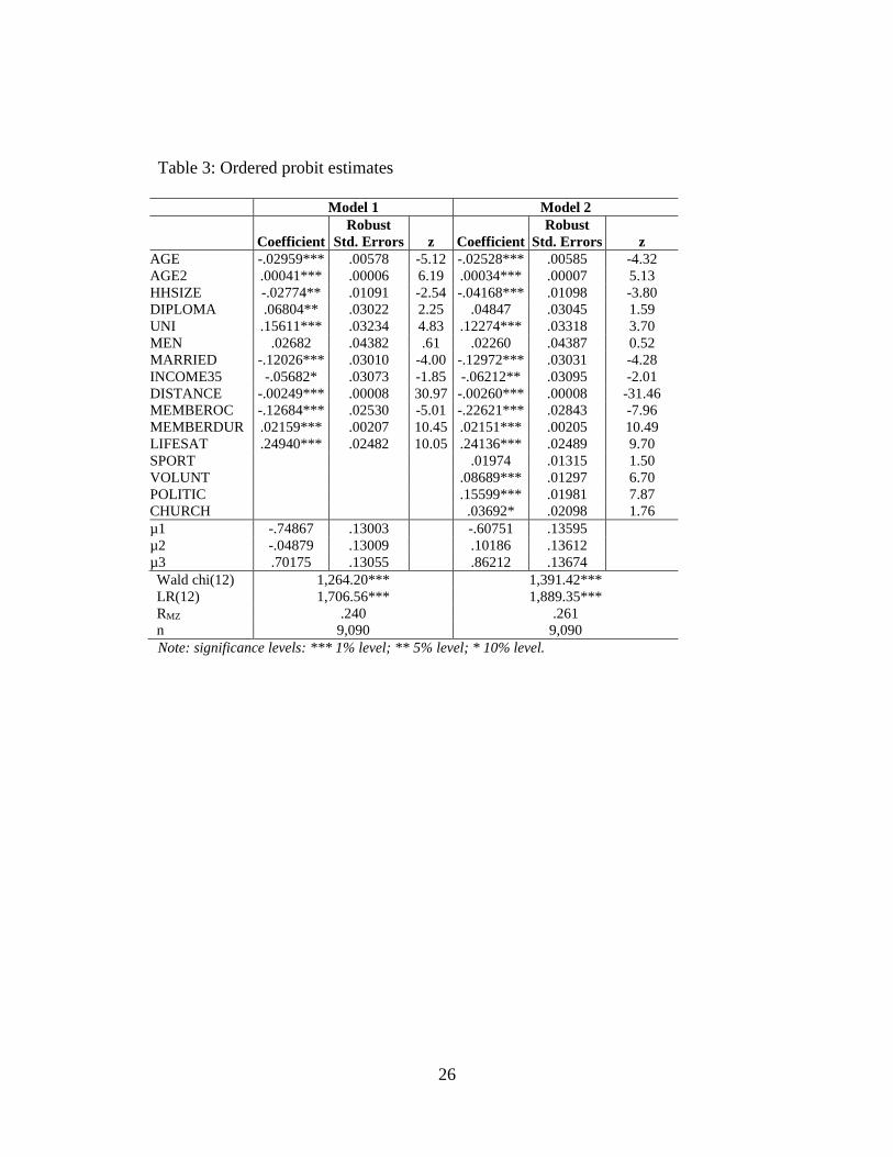
In this section we discuss the results of estimating the model described

above. Table 3 reports regression results for the ordered probit model explaining

persistence of voting behavior by the members of HSV. We estimate the model

both with and without the variables about frequency of sports participation,

volunteerism, political activity, and church. Explanatory variables hold few

surprises, and coefficient estimates are little different between the models with

and without the frequency of other activities variables.

The impact of age on the likelihood of voting is minimized at 36 or 37

years old. Club members younger than this grow less likely to vote as they age,

while club members older that 36 or 37 become more likely to vote as they age.

Consistent with our expectations a greater household size has negative impact on

regular voting while the probability of voting more frequently is increasing with

increasing educational level. In contrast to our expectations, males are not more

likely than females to be voters. However, over 90% of the survey respondents

are male, so it is possible that there are not enough females to estimate a gender

difference. It is also possible that any female that is sufficiently interested in

sport, particularly football, to be a member of the sport club is also sufficiently

interested to participate in club governance at the same rate as the male members

of the club. Distance by car between one’s home and the meeting place is

significantly and negatively related to frequency of voting. The z-score for this

15

variable is 30.97 and 31.46 in the two models, larger in absolute size than that of

any other variable, suggesting distance has quite a strong influence on voting

participation. In addition to these socio-demographic characteristics our setting

specific variables indicate that those voters who are members of more than one

sports club are significantly less likely to vote than are members of just Hamburg

SV. Furthermore, club members are also more likely to vote if they reported that

the success of the club affected their life satisfaction. Finally, each of the four

coefficients on the frequency of activity variables is positive, though sport

participation is not statistically significant at any conventional significance level.

Both volunteerism and political activity are significant at the 1% level and

religious activity is significant at the 10% level.

Consider now the threshold variables. For the model without participation

variables, the first threshold is at -0.749 which means that the probability is 0.227

that a voter’s unexplained motivation for voting, or their benefits from the act of

voting, regardless of the outcome of the vote, are so small that they never vote.

Said differently, 22.7% of voters derive too little benefit from the act of voting for

that to ever induce them to vote. Threshold 2 is -0.049, or at a probability of

0.491. About 25.4% of the voters derive enough benefit from the act of voting

that they will seldom vote rather than never vote. The third threshold, 0.702,

implies that an additional 27.8% of voters are motivated to vote “sometimes” by

the benefits from the act of voting. The remainder indicates that 24.1% of the club

members surveyed would be motivated to vote “often” if only the consumption

benefits of voting mattered. The results are a bit different when the variables for

frequency of participation in other activities are included. The threshold

parameters indicate that 27.1, 26.9, 26.5, and 19.4% of voters fall in the four

categories, respectively. The largest impact is in reducing by about 5 percentage

points the percentage of voters whose utility from voting is sufficiently great as to

induce them to vote often.

16

In the following we provide two examples on how to use this information

on the threshold parameters to derive further conclusions. First, suppose that a

voter were completely indifferent between never voting and seldom voting, that

is, her utility is exactly -0.749. For that voter to become indifferent between

seldom voting and sometimes voting, her utility would have to increase by 0.7 (=-

0.749 - (-0.049)). That gain in utility would require the voter move 281

(=0.7/0.0025) km closer to Hamburg. For that same voter to often vote, she

would have to move more than 582 kilometers closer to Hamburg. The mean

distance from Hamburg for our sample is 177 kilometers, but for those who never

or seldom vote the mean is 213 kilometers, while it is 77 kilometers for those who

sometimes or often vote. Our results suggest that few individuals in our sample

live sufficiently far away that their voting participation would be materially

affected by moving closer to Hamburg.

Second, the negative impact of age on voting is strongest at 36 or 37 years

of age, reducing the utility index about .53 and .47 in models 1 and 2 respectively.

Note that even at the largest impact, the effect of age is not sufficient to change a

voter from indifferent between sometimes voting and seldom voting into

indifferent between seldom and never voting. Likewise, age would never be

sufficient to change someone indifferent between often and sometimes voting into

a seldom voter. At 20 years old, the total impact of age is negative, about -.42 in

model 1 and -.37 in model 2. The results also indicate that while increased age

reduces the negative impact of age on voting after one reaches their mid-30s,

increased age only changes that impact into positive for voters in their 70s, 73 or

older in model 1 and 75 or older in model 2.3

3 Note, that out of n=9,090 individuals in our sample, 42 are 73 years old or older; 10 of these 42

report voting (attending the club annual meeting) often, 9 sometimes.

17

6. Conclusion

This paper has used a unique data set and what we believe is a novel

estimation strategy to address the size of consumption benefits from voting and

the impact of distance/travel cost on the persistence of voter participation. The

model employed is an ordered probit with three threshold parameters dividing the

voters according to the degree to which their voting is based on “civic duty”,

enjoyment from participation in club governance, or genetics, holding all other

things constant.

Our approach seems successful, as the empirical results are intuitive with

most variables being statistically significant: it is found that setting-specific

variables like length of club membership and whether or not the individual

belongs to more than one sport club matter for voting. Furthermore, consistent

with the general turnout literature, age, education level, marital status and

household size also affect participation. In addition, distance from the polling

place statistically significantly influences voting, but may have little practical

impact since few individuals in our sample live sufficiently far away that their

voting participation would be materially affected by moving closer to the venue in

Hamburg where voting takes place.

Although this analysis is not of a typical political environment of a

national, regional or local election we think that our findings are generally

transferable to other elections as argued before. It appears promising to test the

robustness of our results in future research based on other data sets. However, to

the best of our knowledge micro data on repeated general elections is

unfortunately not available at present.

18

References

Cebula, R., & Toma, M. (2006). Determinants of geographical differentials in the

voter participation rate. Atlantic Economic Journal, 34, 33–40.

Coate, S. & Conlin, M. (2004). A Group Rule: Utilitarian Approach to Voter

Turnout: Theory and Evidence. American Economic Review, 94(4), 1476-

1504.

Dietl, H. M. & Franck, E. (2007). Governance failure and financial crisis in

German football. Journal of Sports Economics, 8(6), 662-669.

Downs, A. (1957). An economic theory of democracy. New York: Harper and

Row.

Feddersen, T. and Sandroni, A. (2006). A Theory of Participation in Elections.

American Economic Review, 96(4),1271-1282.

Feddersen, T.J. (2004). Rational Choice Theory and the Paradox of Not Voting.

Journal of Economic Perspectives, 18(1), 99-112.

Fort, R. (1995). A recursive treatment of the hurdles to voting. Public Choice,

85(1-2), 45-69.

Fowler, J.H., Baker, L.A. & Dawes, C.T. (2008). Genetic Variation in Political

Participation. American Political Science Review, 102 (2), 233–48.

Fowler, J.H. & Dawes, C.T. (2008). Two genes predict voter turnout. Journal of

Politics, 70(3):579-594.

Franck, E. (2010). Private Firm, Public Corporation or Member’s Association

Governance Structures in European Football. International Journal of

Sport Finance, 5, 108-127.

Frey, B. (1971). Why do high income people participate more in politics. Public

Choice, 11, 101–105.

Gerber, A.S , Green, D.P. & Shachar, R. (2008). Voting May Be Habit-Forming:

Evidence from a Randomized Field Experiment. American Journal of

Political Science, 47(3), 540-550.

Gibson, J., Kim, B., Stillman, S. & Boe-Gibson (2012). Time to vote? Public

Choice, DOI 10.1007/s11127-011-9909-5

Green, D.P. & Shachar, R. (2000). Habit formation and Political Behaviour:

Evidence of Consuetude in Voter Turnout. British Journal of Political

Science, 30(4), 56-573.

Haspel, M. & Knotts, H. G. (2005). Location, location, location: Precinct

placement and the costs of voting. The Journal of Politics, 67(2), 560-573.

Knack, S. (1994) Does rain help the Republicans? Theory and evidence on

turnout and the vote. Public Choice, 79, 187-209.

19

Ledyard, J. (1981). The Paradox of Voting and Candidate Competition: A General

Equilibrium Analysis, in Essays in Contemporary Fields of Economics.

George Hoorwich and James P. Quick, eds. Lafayette: Purdue University

Press, pp. 54–80.

Ledyard, J. (1984). The Pure Theory of Two Candidate Elections. Public Choice.

44(1), 7–41.

Loewen, P. J. & Dawes, C.T. (2012). The heritability of duty and voter turnout.

Political Psychology, 33(3) ,363-373.

Matsusaka, J. & Palda, F. (1993). The Downsian voter meets the ecological

fallacy. Public Choice, 77(4), 855-878.

Morton, R. (1991). Groups in Rational Turnout Models. American Journal of

Political Science, 35, 758–76.

Mueller, D. (1989). Public Choice II. New York: Cambridge University Press.

Munger, M. (2001) Voting in The Elgar Companion to Public Choice, W. F.

Shughart, II & L. Razzolini, eds. Edward Elgar Publishing: Northampton,

MA.

Niemi, R.G. & Hanmer, M.J. (2010). Voter Turnout Among College Students:

New Data and a Rethinking of Traditional Theories. Social Science

Quarterly, 91(2), 301-323.

Palfrey, T. & Rosenthal, H. (1983). A Strategic Calculus of Voting. Public

Choice. 41(1), 7–53.

Palfrey, T. & Rosenthal, H. (1985). Voter Participation and Strategic Uncertainty.

American Political Science Review, 79(1), 62–78.

Pollock, P.H. III. (1982).”Organizations as Agents of Mobilization: How Does

Group Activity Affect Political Participation?” American Journal of

Political Science, 26(3):486-503.

Powell, G. B. (1986). American Voter Turnout in Comparative Perspective.

American Political Science Review, 80(1), 17–43.

Riker, W. & Ordeshook, P. (1968). A Theory of the Calculus of Voting. American

Political Science Review, 62, 25–42.

Sanders, M.S. (2001). Uncertainty and Turnout. Political Analysis, 9(1), 45-57.

Shachar, R. and Nalebuff, B. (1999). Follow the Leader: Theory and Evidence on

Political Participation. American Economic Review, 89(3), 525–47.

Timpone, R.J. (1998). Structure, Behavior and Voter turnout in the United States.

American Political Science Review, 92(1), 145-158.

Tullock, G. (1967). Towards a Mathematics of Politics. Ann Arbor: University of

Michigan Press.

20

Wolfinger, R. E. and Rosenstone, S. J. (1980). Who Votes? New Haven: Yale

University Press.

21

Figure 1: Comparison between sample (n=9,090) and total population “all

members of HSV aged 16 years and older” (without members living abroad,

N=56,847), focus: 2-digit-ZIP

22

Figure 2: Comparison between sample (n=9,090) and total population “all

members of HSV aged 16 years and older” (N=57,612), focus: age and gender

23

Figure 3: Main reasons for attending the annual assemblies (subsample of

members who attend the assemblies sometimes or often, n=2,404)

24

Table 1: Variable definition

Voter turnout

FREQVOTE Frequency of attending the annual general assembly of HSV (4-

point-scale, 0=never, 1=seldom, 2=sometimes, 3=often)

Socio-demographic characteristics

AGE Age (in years)

AGE2 Age (in years) squared

HHSIZE Household size

DIPLOMA Educational level (dummy, final secondary school examination=1)

UNI Educational level (dummy, university’s degree=1)

MEN Gender (dummy, male=1)

MARRIED Family status (dummy, married=1)

INCOME35

DISTANCE

Income is at or above 3,500 Euros per month

Travel distance to the assembly venue by car (in kilometer)

Membership characteristics

MEMBEROC Member in another sport club (member=1)

MEMBERDUR Length of the HSV membership (in years)

LIFESAT The performance of HSV has an impact on my overall life

satisfaction (dummy, I agree or tend to agree=1)

Leisure time engagement

SPORT Frequency of physical activity (4-point-scale, 0=never…3=each

week)

VOLUNT Frequency of volunteerism in sport clubs or for community services

(4-point-scale, 0=never…3=each week)

POLITIC Frequency of engagement with political parties or citizens’ groups

(4-point-scale, 0=never…3=each week)

CHURCH Frequency of church attendance (4-point-scale, 0=never…3=each

week)

25

Table 2: Descriptive statistics: (conditional) mean values and t-test significances

mean

mean if

FREQVOTE=2 or 3

mean if

FREQVOTE=0 or 1

FREQVOTE .857*** 2.367 .314

AGE 40.838* 41.198 40.708

HHSIZE 2.681*** 2.554 2.726

DIPLOMA .266* .277 .262

UNI .238*** .256 .231

MEN .902** .891 .906

MARRIED .484*** .435 .501

INCOME35 .278 .269 .282

DISTANCE 177.333*** 76.646 213.536

MEMBEROC .410*** .342 .435

MEMBERDUR 6.939*** 8.028 6.547

LIFESAT .459*** .505 .443

SPORT 2.129 2.119 2.133

VOLUNT 1.127** 1.168 1.112

POLITIC .333*** .411 .304

CHURCH .390* .406 .383

n 9,090 2,404 6,686

Note: significance levels of the t-test: *** 1% level; ** 5% level; * 10% level.

26

Table 3: Ordered probit estimates

Model 1 Model 2

Coefficient

Robust

Std. Errors

z Coefficient

Robust

Std. Errors

z

AGE -.02959*** .00578 -5.12 -.02528*** .00585 -4.32

AGE2 .00041*** .00006 6.19 .00034*** .00007 5.13

HHSIZE -.02774** .01091 -2.54 -.04168*** .01098 -3.80

DIPLOMA .06804** .03022 2.25 .04847 .03045 1.59

UNI .15611*** .03234 4.83 .12274*** .03318 3.70

MEN .02682 .04382 .61 .02260 .04387 0.52

MARRIED -.12026*** .03010 -4.00 -.12972*** .03031 -4.28

INCOME35 -.05682* .03073 -1.85 -.06212** .03095 -2.01

DISTANCE -.00249*** .00008 30.97 -.00260*** .00008 -31.46

MEMBEROC -.12684*** .02530 -5.01 -.22621*** .02843 -7.96

MEMBERDUR .02159*** .00207 10.45 .02151*** .00205 10.49

LIFESAT .24940*** .02482 10.05 .24136*** .02489 9.70

SPORT .01974 .01315 1.50

VOLUNT .08689*** .01297 6.70

POLITIC .15599*** .01981 7.87

CHURCH .03692* .02098 1.76

µ1 -.74867 .13003 -.60751 .13595

µ2 -.04879 .13009 .10186 .13612

µ3 .70175 .13055 .86212 .13674

Wald chi(12) 1,264.20*** 1,391.42***

LR(12) 1,706.56*** 1,889.35***

RMZ .240 .261

n 9,090 9,090

Note: significance levels: *** 1% level; ** 5% level; * 10% level.