The geometry of nesting problems: A tutorial - vmk.ugatu.ac.ruvmk.ugatu.ac.ru/c&p/article/new/nesting_problems_tutorialEJOR-184... · The geometry of nesting problems: A tutorial

European Journal of Operational Research 184 (2008) 397–415

www.elsevier.com/locate/ejor

Invited Tutorial

The geometry of nesting problems: A tutorial

Julia A. Bennell a,*, Jose F. Oliveira b,c

a Centre for Operations Research, Management Science and Information Systems, University of Southampton,

Highfield, Southampton SO17 1BJ, UKb Faculdade de Engenharia da Universidade do Porto, Portugal

c INESC Porto – Instituto de Engenharia de Sistemas e Computadores do Porto, Portugal Rua Dr. Roberto Frias,

4200-465 Porto, Portugal

Received 20 July 2006; accepted 15 November 2006Available online 31 December 2006

Abstract

Cutting and packing problems involving irregular shapes is an important problem variant with a wide variety of indus-trial applications. Despite its relevance to industry, research publications are relatively low when compared to other cuttingand packing problems. One explanation offered is the perceived difficulty and substantial time investment of developing ageometric tool box to assess computer generated solutions. In this paper we set out to provide a tutorial covering the coregeometric methodologies currently employed by researchers in cutting and packing of irregular shapes. The paper is notdesigned to be an exhaustive survey of the literature but instead will draw on the literature to illustrate the theory andimplementation of the approaches. We aim to provide a sufficiently instructive description to equip new and currentresearchers in the area to select the most appropriate methodology for their needs.� 2007 Elsevier B.V. All rights reserved.

Keywords: Cutting; Packing; Geometry; Optimisation

1. Introduction

Cutting and packing problems involving irregu-lar shapes arise in a wide variety of industriesincluding; garment manufacturing, sheet metal cut-ting, furniture making and shoe manufacturing.An example of a layout from the garment manufac-turing industry is provided in Fig. 1. As a result therange of problem variants involving irregularshapes, referred to here as nesting problems, is a

0377-2217/$ - see front matter � 2007 Elsevier B.V. All rights reserved

doi:10.1016/j.ejor.2006.11.038

* Corresponding author. Tel.: +23 80595671; fax: +23805933844.

E-mail addresses: [email protected] (J.A. Bennell),[email protected] (J.F. Oliveira).

core area of research in the field of cutting andpacking. The problem is NP-complete and as aresult solution methodologies predominantly utiliseheuristics. A further defining characteristic of nest-ing problems is the requirement to develop power-ful geometric tools to handle the wide variety andcomplexity of shapes that need to be packed. Inthis paper we propose to provide detailed explana-tions of the most popular techniques for handlingthe geometry when solving nesting problems andprovide guidance on their implementation, strengthsand weaknesses.

The remainder of this paper is organized in sixsections. In the next section the nesting problem isdefined more precisely and the key differences

.

mailto:[email protected]

mailto:[email protected]

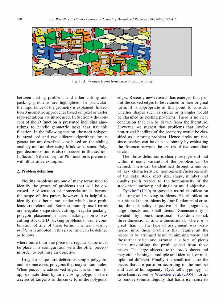
Fig. 1. An example layout from garment manufacturing.

398 J.A. Bennell, J.F. Oliveira / European Journal of Operational Research 184 (2008) 397–415

between nesting problems and other cutting andpacking problems are highlighted. In particular,the importance of the geometry is explained. In Sec-tion 3 geometric approaches based on pixel or rasterrepresentations are introduced. In Section 4 the con-cept of the D function is presented including algo-rithms to handle geometric tasks that use thisfunction. In the following section, the nofit polygonis introduced and two different algorithms for itsgeneration are described, one based on the slidinganalogy and another using Minkowski sums. Poly-gon decomposition is also discussed in this section.In Section 6 the concept of Phi function is presentedwith illustrative examples.

2. Problem definition

Nesting problems are one of many terms used toidentify the group of problems that will be dis-cussed. A discussion of nomenclature is beyondthe scope of this paper, however, it is helpful toidentify the other names under which these prob-lems are referenced. Some commonly used termsare irregular shape stock cutting, irregular packing,polygon placement, marker making, non-convexcutting stock, 2-D packing problems or some com-bination of any of these terms. The term nesting

problems is adopted in this paper and can be definedas follows:

where more than one piece of irregular shape mustbe place in a configuration with the other piece(s)in order to optimise an objective

Irregular shapes are defined as simple polygons,and in some cases, polygons that may contain holes.When pieces include curved edges, it is common toapproximate them by an enclosing polygon, wherea series of tangents to the curve form the polygonal

edges. Recently new research has emerged that per-mit the curved edges to be retained in their originalform. It is appropriate at this point to considerwhether shapes such as circles or triangles wouldbe classified as nesting problems. There is no clearconclusion that can be drawn from the literature.However, we suggest that problems that involvenon-trivial handling of the geometry would be clas-sified as a nesting problem. Hence circles are not,since overlap can be detected simply by evaluatingthe distance between the centres of two candidatecircles.

The above definition is clearly very general andwithin it many variants of the problem can bedefined. These can be identified through a numberof key characteristics; homogeneity/heterogeneityof the data; stock sheet size, shape, number andquality (with respect to the homogeneity of thestock sheet surface); and single or multi objective.

Dyckhoff (1990) proposed a useful classificationof cutting and packing problems. His classificationpartitioned the problems by four fundamental crite-ria; dimensionality, objective of the assignment,large objects and small items. Dimensionality isdivided by one-dimensional, two-dimensional,three-dimensional and n-dimensional, where n isgreat than 3. The type of assignment was parti-tioned into: those problems that require all thepieces to be arranged hence minimising waste andthose that select and arrange a subset of pieceshence maximising the profit gained from thosepieces. The large objects are the stock sheets andmay either be single, multiple and identical, or mul-tiple and different. Finally, the small items are thepieces that are partition according to the numberand level of homogeneity. Dyckhoff’s typology hassince been revised by Waescher et al. (2005) in orderto remove some ambiguity that has arisen since its

J.A. Bennell, J.F. Oliveira / European Journal of Operational Research 184 (2008) 397–415 399

publication and provide a more intuitive classifica-tion of problem variants. Their typology retainsthe first two detailed by Dyckhoff; dimensionalityand objective of the assignment. The categories forlarge object and small objects are redefined, and anew characteristic is identified; shape of the smallitems. Using Waescher, Hauber and Schumann’stypology, nesting problems, in general, would beplaced in the open-dimension problem category, withthe refinement of being two-dimensional and irregu-lar. The new typology provides a useful progressiontowards a consistent nomenclature for cutting andpacking problems.

2.1. How is nesting different from other cutting and

packing problems?

A comparison of the physical attributes of cut-ting and packing problems in order to group themhas already been addressed through the discussionof the typology. Here we are interested in the two-dimensional problems, which can be further parti-tioned into regular packing and irregular packing.These differences are tangible and observable; per-haps the more important question is how these dif-ferences influence the approaches we might take tosolve the problem. The paper will discuss theincreased complexity of ensuring pieces are allo-cated to feasible placement position when they areirregular. However, simply deriving more sophisti-cated feasibility tests may not be sufficient to modifya successful rectangle packing approach to also besuccessful for irregular shapes.

Although there are an infinite number of differentrectangles with respect to their size and ratio oflength and width, the fact that all pieces are rectan-gular allows you to cut down the potential place-ment positions to a finite set. Where as the infinitevariety of sizes and shapes of simple polygons pro-vide a much greater challenge. In the case of rectan-gular pieces, it is easy to reduce the stock sheet to adiscrete set of candidate locations by defining a gridof feasible placement positions by the largest com-mon divisor of all the rectangular edges. The sameapproach can be applied for instances where thepieces only contain edges that are orthogonal toeach other and the edges of the stock sheet. How-ever, if this is not the case then defining such a gridcan remove good solutions from the solutions space.Hence, in all but the orthogonal case describedabove, the stock sheet is continuous and for eachpiece in the data set the number of feasible place-

ment positions on the stock sheet is infinite. As aresult, an implementation for nesting problems hasto embed mechanisms into the approach for reduc-ing the solution space, preferably without removingthe best solutions. In addition to the increasedcomplexity of the solution space, the calculation offeasibility of the solution is significantly more com-putationally intensive. Hence, many fewer solutionsmay be evaluated in the same run time. Other differ-ences worth noting are that bounds can be moreeasily found for rectangular problems (e.g. Beasley,1985; Letchford and Amaral, 2001; Y and Kang,2002) and potentially any rotation of the piecesmay be considered.

2.2. Why is the geometry important?

The most visible attribute of nesting problemsand the first obstacle researchers come up againstis the geometry. By this we mean answering thequestion; given a position on the stock sheet oftwo pieces, does this result in them overlapping,touching, or are they separated? The answer to thisquestion is trivial to the human eye. To write a com-puter programme to determine this information ismuch more complex since the answer can only befound from processing a set of vertices or in somecases categories of pixels. Developing a set of toolsto assimilate the geometry is a non-trivial task andpotentially a barrier that stifles academic researchin this area. There exist a number of solutions tothis problem ranging from simple to complex. How-ever, each has their idiosyncrasies. Determiningwhich is the most appropriate approach to imple-ment is not just a matter of how well they perform,but also how difficult they are to implementrobustly. Also the selected approach for solvingthe nesting problem will impact the level of benefitfrom time invested in implementing and pre-pro-cessing highly efficient geometric tools. The remain-der of this paper is dedicated to describing the mostcommon approaches found in the literature, theseare; the raster method, direct trigonometry, the nofitpolygon and the phi function.

3. Pixel/raster method

Raster methods are approaches that divide thecontinuous stock sheet into discrete areas, hencereducing the geometric information to coding thedata by a grid represented by a matrix. However,different authors have used different codification


schemes, which are largely driven by the place-ment algorithm that will use this geometric infor-mation.

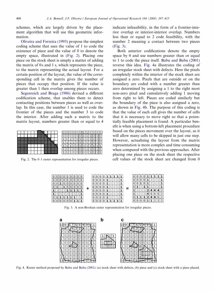
Oliveira and Ferreira (1993) propose the simplestcoding scheme that uses the value of 1 to code theexistence of piece and the value of 0 to denote theempty space, illustrated in (Fig. 2). Placing onepiece on the stock sheet is simply a matter of addingthe matrix of 0s and 1 s, which represents the piece,to the matrix representing the actual layout. For acertain position of the layout, the value of the corre-sponding cell in the matrix gives the number ofpieces that occupy that position. If the value isgreater than 1 then overlap among pieces occurs.

Segenreich and Braga (1986) devised a differentcodification scheme, that enables them to detectcontacting positions between pieces as well as over-lap. In this case, the number 1 is used to code thefrontier of the pieces and the number 3 to codethe interior. After adding such a matrix to thematrix layout, numbers greater than or equal to 4

Fig. 2. The 0–1 raster representation for irregular pieces.

Fig. 3. A non-Boolean raster repre

Fig. 4. Raster method proposed by Babu and Babu (2001): (a) stock sh

indicate infeasibility, in the form of a frontier-inte-rior overlap or interior-interior overlap. Numbersless than or equal to 2 code feasibility, with thenumber 2 meaning a contact between two pieces(Fig. 3).

Both anterior codifications denote the emptyspace by 0 and use numbers greater than or equalto 1 to code the piece itself. Babu and Babu (2001)reverse this idea. Fig. 4a illustrates the coding ofan irregular stock sheet with defects. Here the pixelscompletely within the interior of the stock sheet areassigned a zero. Pixels that are outside or on theboundary are coded with a number greater thanzero determined by assigning a 1 to the right mostnon-zero pixel and cumulatively adding 1 movingfrom right to left. Pieces are coded similarly butthe boundary of the piece is also assigned a zero,as shown in Fig. 4b. The purpose of this coding isthat the value of each cell gives the number of cellsthat it is necessary to move right so that a poten-tially feasible placement is found. A particular ben-efit is when using a bottom-left placement procedurebased on the pieces movement over the layout, as itwill allow many cells to be skipped in just one step.However, actualising the layout from the matrixrepresentation is more complex and time consumingwhen compared with the previous approaches. Afterplacing one piece on the stock sheet the respectivecell values of the stock sheet are changed from 0

sentation for irregular pieces.

eet with defects, (b) piece and (c) stock sheet with a piece placed.

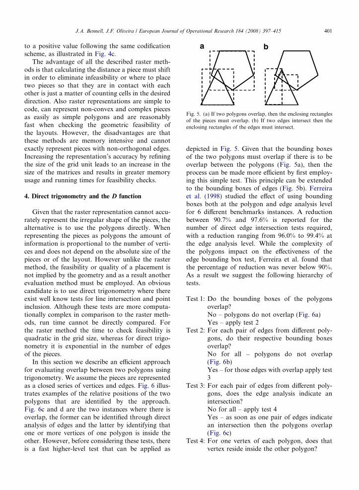
Fig. 5. (a) If two polygons overlap, then the enclosing rectanglesof the pieces must overlap. (b) If two edges intersect then theenclosing rectangles of the edges must intersect.


to a positive value following the same codificationscheme, as illustrated in Fig. 4c.

The advantage of all the described raster meth-ods is that calculating the distance a piece must shiftin order to eliminate infeasibility or where to placetwo pieces so that they are in contact with eachother is just a matter of counting cells in the desireddirection. Also raster representations are simple tocode, can represent non-convex and complex piecesas easily as simple polygons and are reasonablyfast when checking the geometric feasibility ofthe layouts. However, the disadvantages are thatthese methods are memory intensive and cannotexactly represent pieces with non-orthogonal edges.Increasing the representation’s accuracy by refiningthe size of the grid unit leads to an increase in thesize of the matrices and results in greater memoryusage and running times for feasibility checks.

4. Direct trigonometry and the D function

Given that the raster representation cannot accu-rately represent the irregular shape of the pieces, thealternative is to use the polygons directly. Whenrepresenting the pieces as polygons the amount ofinformation is proportional to the number of verti-ces and does not depend on the absolute size of thepieces or of the layout. However unlike the rastermethod, the feasibility or quality of a placement isnot implied by the geometry and as a result anotherevaluation method must be employed. An obviouscandidate is to use direct trigonometry where thereexist well know tests for line intersection and pointinclusion. Although these tests are more computa-tionally complex in comparison to the raster meth-ods, run time cannot be directly compared. Forthe raster method the time to check feasibility isquadratic in the grid size, whereas for direct trigo-nometry it is exponential in the number of edgesof the pieces.

In this section we describe an efficient approachfor evaluating overlap between two polygons usingtrigonometry. We assume the pieces are representedas a closed series of vertices and edges. Fig. 6 illus-trates examples of the relative positions of the twopolygons that are identified by the approach.Fig. 6c and d are the two instances where there isoverlap, the former can be identified through directanalysis of edges and the latter by identifying thatone or more vertices of one polygon is inside theother. However, before considering these tests, thereis a fast higher-level test that can be applied as

depicted in Fig. 5. Given that the bounding boxesof the two polygons must overlap if there is to beoverlap between the polygons (Fig. 5a), then theprocess can be made more efficient by first employ-ing this simple test. This principle can be extendedto the bounding boxes of edges (Fig. 5b). Ferreiraet al. (1998) studied the effect of using boundingboxes both at the polygon and edge analysis levelfor 6 different benchmarks instances. A reductionbetween 90.7% and 97.6% is reported for thenumber of direct edge intersection tests required,with a reduction ranging from 96.0% to 99.4% atthe edge analysis level. While the complexity ofthe polygons impact on the effectiveness of theedge bounding box test, Ferreira et al. found thatthe percentage of reduction was never below 90%.As a result we suggest the following hierarchy oftests.

Test 1: Do the bounding boxes of the polygonsoverlap?
No – polygons do not overlap (Fig. 6a)Yes – apply test 2
Test 2: For each pair of edges from different poly-gons, do their respective bounding boxesoverlap?
No for all – polygons do not overlap(Fig. 6b)Yes – for those edges with overlap apply test3
Test 3: For each pair of edges from different poly-gons, does the edge analysis indicate anintersection?
No for all – apply test 4Yes – as soon as one pair of edges indicatean intersection then the polygons overlap(Fig. 6c)
Test 4: For one vertex of each polygon, does thatvertex reside inside the other polygon?

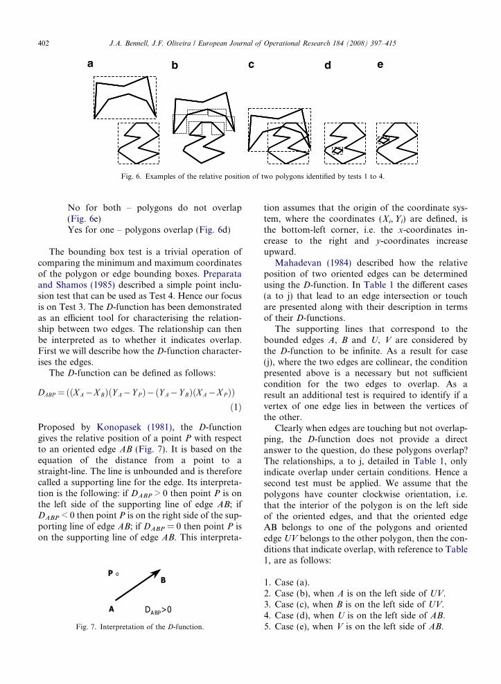
Fig. 6. Examples of the relative position of two polygons identified by tests 1 to 4.


No for both – polygons do not overlap(Fig. 6e)Yes for one – polygons overlap (Fig. 6d)

The bounding box test is a trivial operation ofcomparing the minimum and maximum coordinatesof the polygon or edge bounding boxes. Preparataand Shamos (1985) described a simple point inclu-sion test that can be used as Test 4. Hence our focusis on Test 3. The D-function has been demonstratedas an efficient tool for characterising the relation-ship between two edges. The relationship can thenbe interpreted as to whether it indicates overlap.First we will describe how the D-function character-ises the edges.

The D-function can be defined as follows:

DABP ¼ððX A�X BÞðY A�Y P Þ�ðY A�Y BÞðX A�X P ÞÞð1Þ

Proposed by Konopasek (1981), the D-functiongives the relative position of a point P with respectto an oriented edge AB (Fig. 7). It is based on theequation of the distance from a point to astraight-line. The line is unbounded and is thereforecalled a supporting line for the edge. Its interpreta-tion is the following: if DABP > 0 then point P is onthe left side of the supporting line of edge AB; ifDABP < 0 then point P is on the right side of the sup-porting line of edge AB; if DABP = 0 then point P ison the supporting line of edge AB. This interpreta-

Fig. 7. Interpretation of the D-function.

tion assumes that the origin of the coordinate sys-tem, where the coordinates (Xi,Yi) are defined, isthe bottom-left corner, i.e. the x-coordinates in-crease to the right and y-coordinates increaseupward.

Mahadevan (1984) described how the relativeposition of two oriented edges can be determinedusing the D-function. In Table 1 the different cases(a to j) that lead to an edge intersection or touchare presented along with their description in termsof their D-functions.

The supporting lines that correspond to thebounded edges A, B and U, V are considered bythe D-function to be infinite. As a result for case(j), where the two edges are collinear, the conditionpresented above is a necessary but not sufficientcondition for the two edges to overlap. As aresult an additional test is required to identify if avertex of one edge lies in between the vertices ofthe other.

Clearly when edges are touching but not overlap-ping, the D-function does not provide a directanswer to the question, do these polygons overlap?The relationships, a to j, detailed in Table 1, onlyindicate overlap under certain conditions. Hence asecond test must be applied. We assume that thepolygons have counter clockwise orientation, i.e.that the interior of the polygon is on the left sideof the oriented edges, and that the oriented edgeAB belongs to one of the polygons and orientededge UV belongs to the other polygon, then the con-ditions that indicate overlap, with reference to Table1, are as follows:

1. Case (a).2. Case (b), when A is on the left side of UV.3. Case (c), when B is on the left side of UV.4. Case (d), when U is on the left side of AB.5. Case (e), when V is on the left side of AB.

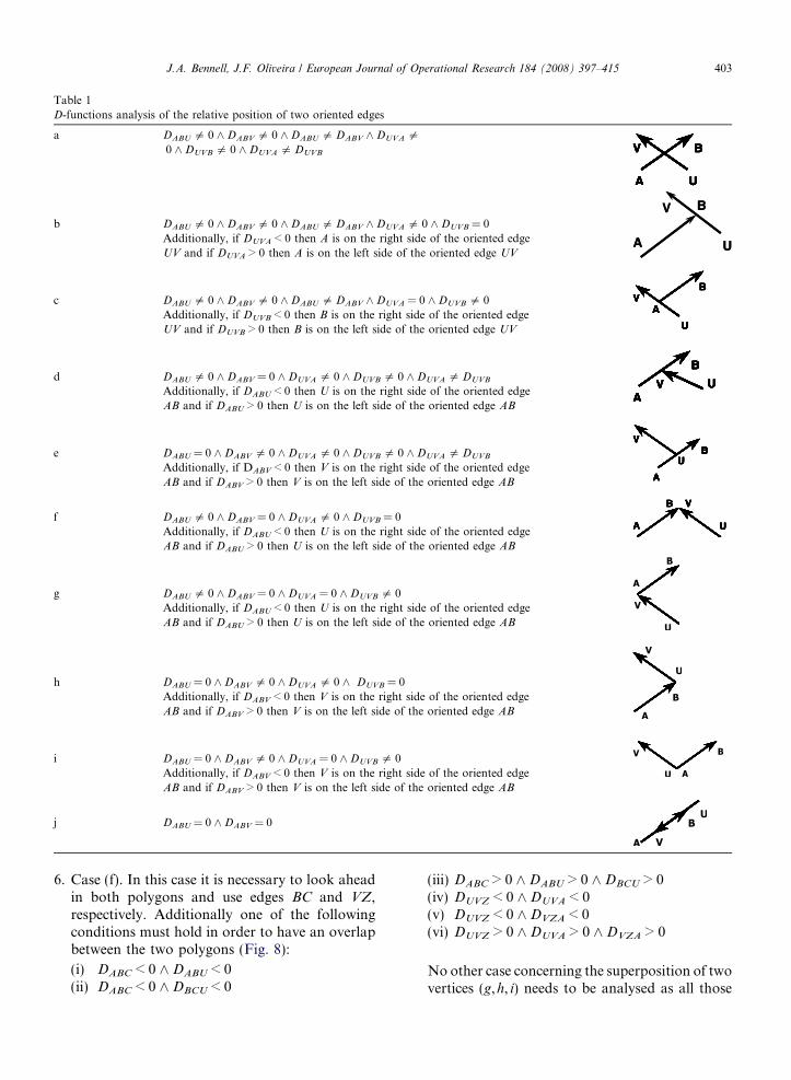
Table 1D-functions analysis of the relative position of two oriented edges

a DABU 5 0 ^ DABV 5 0 ^ DABU 5 DABV ^ DUVA 5

0 ^ DUVB 5 0 ^ DUVA 5 DUVB

A

B

U

V

A

B

U

V

A

B

U

V

A

B

U

V

A

B

U

V

A

B

U

V

A

B

U

V

b DABU 5 0 ^ DABV 5 0 ^ DABU 5 DABV ^ DUVA 5 0 ^ DUVB = 0Additionally, if DUVA < 0 then A is on the right side of the oriented edgeUV and if DUVA > 0 then A is on the left side of the oriented edge UV

A

B

U

V

A

B

U

V

c DABU 5 0 ^ DABV 5 0 ^ DABU 5 DABV ^ DUVA = 0 ^ DUVB 5 0Additionally, if DUVB < 0 then B is on the right side of the oriented edgeUV and if DUVB > 0 then B is on the left side of the oriented edge UV

A

B

U

VA

B

U

VA

B

U

VA

B

U

VA

B

U

VA

B

U

VA

B

U

V

d DABU 5 0 ^ DABV = 0 ^ DUVA 5 0 ^ DUVB 5 0 ^ DUVA 5 DUVB

Additionally, if DABU < 0 then U is on the right side of the oriented edgeAB and if DABU > 0 then U is on the left side of the oriented edge AB

A

B

UVA

B

UVA

B

UVA

B

UVA

B

UVA

B

UVA

B

UV

e DABU = 0 ^ DABV 5 0 ^ DUVA 5 0 ^ DUVB 5 0 ^ DUVA 5 DUVB

Additionally, if DABV < 0 then V is on the right side of the oriented edgeAB and if DABV > 0 then V is on the left side of the oriented edge AB A

BU

V

A

BU

V

A

BU

V

A

BU

V

A

BU

V

A

BU

V

A

BU

V

f DABU 5 0 ^ DABV = 0 ^ DUVA 5 0 ^ DUVB = 0Additionally, if DABU < 0 then U is on the right side of the oriented edgeAB and if DABU > 0 then U is on the left side of the oriented edge AB

A

B

U

V

A

B

U

V

A

B

U

V

A

B

U

V

A

B

U

V

A

B

U

V

A

B V

g DABU 5 0 ^ DABV = 0 ^ DUVA = 0 ^ DUVB 5 0Additionally, if DABU < 0 then U is on the right side of the oriented edgeAB and if DABU > 0 then U is on the left side of the oriented edge AB

h DABU = 0 ^ DABV 5 0 ^ DUVA 5 0 ^ DUVB = 0Additionally, if DABV < 0 then V is on the right side of the oriented edgeAB and if DABV > 0 then V is on the left side of the oriented edge AB

i DABU = 0 ^ DABV 5 0 ^ DUVA = 0 ^ DUVB 5 0Additionally, if DABV < 0 then V is on the right side of the oriented edgeAB and if DABV > 0 then V is on the left side of the oriented edge AB

j DABU = 0 ^ DABV = 0


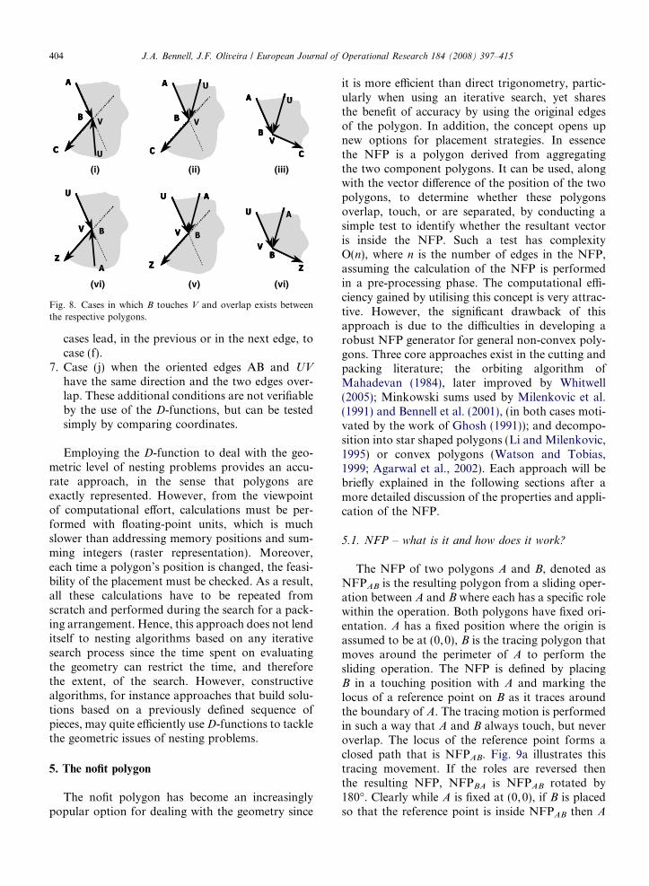
6. Case (f). In this case it is necessary to look aheadin both polygons and use edges BC and VZ,respectively. Additionally one of the followingconditions must hold in order to have an overlapbetween the two polygons (Fig. 8):

(i) DABC < 0 ^ DABU < 0(ii) DABC < 0 ^ DBCU < 0

(iii) DABC > 0 ^ DABU > 0 ^ DBCU > 0(iv) DUVZ < 0 ^ DUVA < 0(v) DUVZ < 0 ^ DVZA < 0(vi) DUVZ > 0 ^ DUVA > 0 ^ DVZA > 0

No other case concerning the superposition of twovertices (g,h, i) needs to be analysed as all those

(i) (ii) (iii)

(vi) (v) (vi)

Fig. 8. Cases in which B touches V and overlap exists betweenthe respective polygons.


cases lead, in the previous or in the next edge, tocase (f).

7. Case (j) when the oriented edges AB and UV

have the same direction and the two edges over-lap. These additional conditions are not verifiableby the use of the D-functions, but can be testedsimply by comparing coordinates.

Employing the D-function to deal with the geo-metric level of nesting problems provides an accu-rate approach, in the sense that polygons areexactly represented. However, from the viewpointof computational effort, calculations must be per-formed with floating-point units, which is muchslower than addressing memory positions and sum-ming integers (raster representation). Moreover,each time a polygon’s position is changed, the feasi-bility of the placement must be checked. As a result,all these calculations have to be repeated fromscratch and performed during the search for a pack-ing arrangement. Hence, this approach does not lenditself to nesting algorithms based on any iterativesearch process since the time spent on evaluatingthe geometry can restrict the time, and thereforethe extent, of the search. However, constructivealgorithms, for instance approaches that build solu-tions based on a previously defined sequence ofpieces, may quite efficiently use D-functions to tacklethe geometric issues of nesting problems.

5. The nofit polygon

The nofit polygon has become an increasinglypopular option for dealing with the geometry since

it is more efficient than direct trigonometry, partic-ularly when using an iterative search, yet sharesthe benefit of accuracy by using the original edgesof the polygon. In addition, the concept opens upnew options for placement strategies. In essencethe NFP is a polygon derived from aggregatingthe two component polygons. It can be used, alongwith the vector difference of the position of the twopolygons, to determine whether these polygonsoverlap, touch, or are separated, by conducting asimple test to identify whether the resultant vectoris inside the NFP. Such a test has complexityO(n), where n is the number of edges in the NFP,assuming the calculation of the NFP is performedin a pre-processing phase. The computational effi-ciency gained by utilising this concept is very attrac-tive. However, the significant drawback of thisapproach is due to the difficulties in developing arobust NFP generator for general non-convex poly-gons. Three core approaches exist in the cutting andpacking literature; the orbiting algorithm ofMahadevan (1984), later improved by Whitwell(2005); Minkowski sums used by Milenkovic et al.(1991) and Bennell et al. (2001), (in both cases moti-vated by the work of Ghosh (1991)); and decompo-sition into star shaped polygons (Li and Milenkovic,1995) or convex polygons (Watson and Tobias,1999; Agarwal et al., 2002). Each approach will bebriefly explained in the following sections after amore detailed discussion of the properties and appli-cation of the NFP.

5.1. NFP – what is it and how does it work?

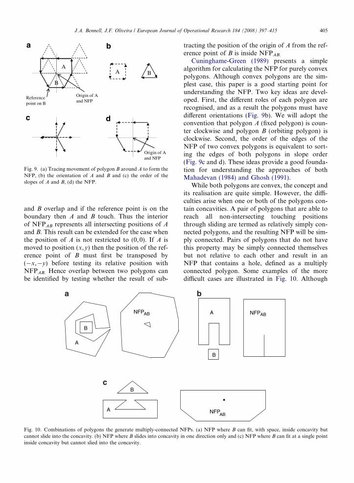
The NFP of two polygons A and B, denoted asNFPAB is the resulting polygon from a sliding oper-ation between A and B where each has a specific rolewithin the operation. Both polygons have fixed ori-entation. A has a fixed position where the origin isassumed to be at (0,0), B is the tracing polygon thatmoves around the perimeter of A to perform thesliding operation. The NFP is defined by placingB in a touching position with A and marking thelocus of a reference point on B as it traces aroundthe boundary of A. The tracing motion is performedin such a way that A and B always touch, but neveroverlap. The locus of the reference point forms aclosed path that is NFPAB. Fig. 9a illustrates thistracing movement. If the roles are reversed thenthe resulting NFP, NFPBA is NFPAB rotated by180�. Clearly while A is fixed at (0, 0), if B is placedso that the reference point is inside NFPAB then A

BA

A

B

Origin of Aand NFP

Reference point on B

Origin of Aand NFP

Fig. 9. (a) Tracing movement of polygon B around A to form theNFP, (b) the orientation of A and B and (c) the order of theslopes of A and B, (d) the NFP.


and B overlap and if the reference point is on theboundary then A and B touch. Thus the interiorof NFPAB represents all intersecting positions of A

and B. This result can be extended for the case whenthe position of A is not restricted to (0, 0). If A ismoved to position (x,y) then the position of the ref-erence point of B must first be transposed by(�x,�y) before testing its relative position withNFPAB. Hence overlap between two polygons canbe identified by testing whether the result of sub-

NFPAB

A

A

B

B

a

c

Fig. 10. Combinations of polygons the generate multiply-connected Ncannot slide into the concavity. (b) NFP where B slides into concavity iinside concavity but cannot slied into the concavity.

tracting the position of the origin of A from the ref-erence point of B is inside NFPAB.

Cuninghame-Green (1989) presents a simplealgorithm for calculating the NFP for purely convexpolygons. Although convex polygons are the sim-plest case, this paper is a good starting point forunderstanding the NFP. Two key ideas are devel-oped. First, the different roles of each polygon arerecognised, and as a result the polygons must havedifferent orientations (Fig. 9b). We will adopt theconvention that polygon A (fixed polygon) is coun-ter clockwise and polygon B (orbiting polygon) isclockwise. Second, the order of the edges of theNFP of two convex polygons is equivalent to sort-ing the edges of both polygons in slope order(Fig. 9c and d). These ideas provide a good founda-tion for understanding the approaches of bothMahadevan (1984) and Ghosh (1991).

While both polygons are convex, the concept andits realisation are quite simple. However, the diffi-culties arise when one or both of the polygons con-tain concavities. A pair of polygons that are able toreach all non-intersecting touching positionsthrough sliding are termed as relatively simply con-nected polygons, and the resulting NFP will be sim-ply connected. Pairs of polygons that do not havethis property may be simply connected themselvesbut not relative to each other and result in anNFP that contains a hole, defined as a multiplyconnected polygon. Some examples of the moredifficult cases are illustrated in Fig. 10. Although

B

A NFPAB

NFPAB

b

FPs. (a) NFP where B can fit, with space, inside concavity butn one direction only and (c) NFP where B can fit at a single point

AA


the example in Fig. 10b is not strictly multiply con-nected, it is included here to illustrate another of themore difficult cases for generating the NFP.

BB

Fig. 12. Sliding edge of A projected from vertices of B to findminimum intersection distance.

5.2. Sliding algorithm

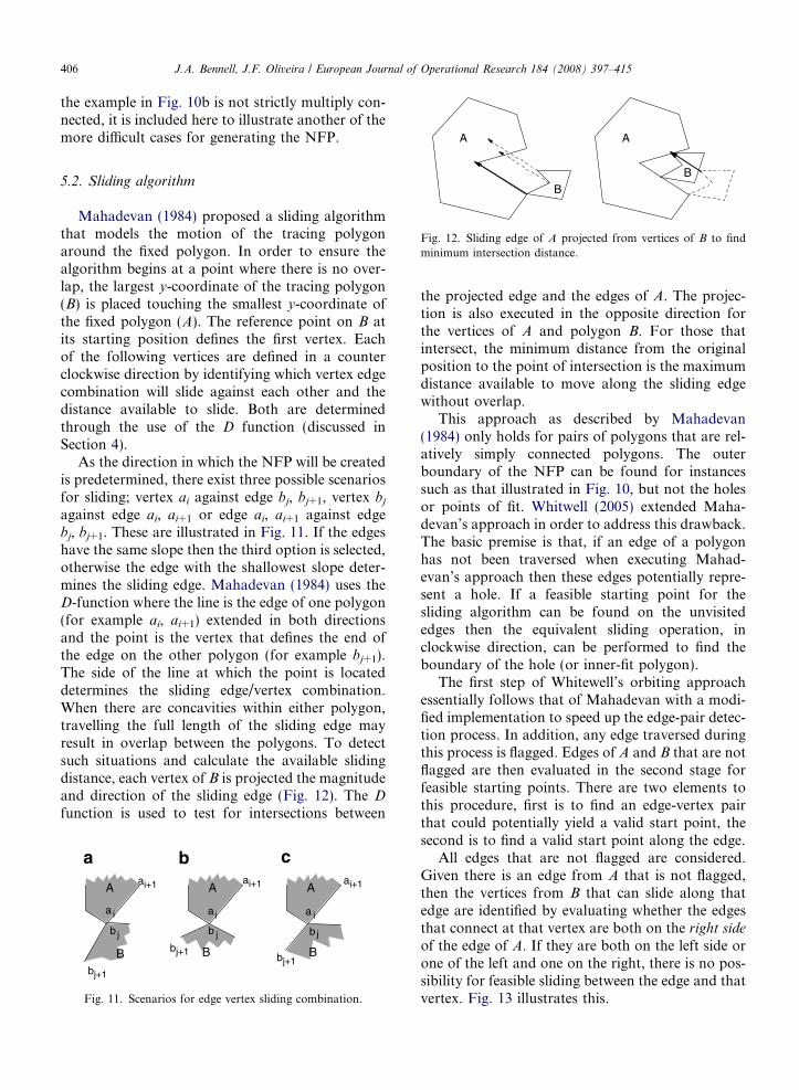
Mahadevan (1984) proposed a sliding algorithmthat models the motion of the tracing polygonaround the fixed polygon. In order to ensure thealgorithm begins at a point where there is no over-lap, the largest y-coordinate of the tracing polygon(B) is placed touching the smallest y-coordinate ofthe fixed polygon (A). The reference point on B atits starting position defines the first vertex. Eachof the following vertices are defined in a counterclockwise direction by identifying which vertex edgecombination will slide against each other and thedistance available to slide. Both are determinedthrough the use of the D function (discussed inSection 4).

As the direction in which the NFP will be createdis predetermined, there exist three possible scenariosfor sliding; vertex ai against edge bj, bj+1, vertex bj

against edge ai, ai+1 or edge ai, ai+1 against edgebj, bj+1. These are illustrated in Fig. 11. If the edgeshave the same slope then the third option is selected,otherwise the edge with the shallowest slope deter-mines the sliding edge. Mahadevan (1984) uses theD-function where the line is the edge of one polygon(for example ai, ai+1) extended in both directionsand the point is the vertex that defines the end ofthe edge on the other polygon (for example bj+1).The side of the line at which the point is locateddetermines the sliding edge/vertex combination.When there are concavities within either polygon,travelling the full length of the sliding edge mayresult in overlap between the polygons. To detectsuch situations and calculate the available slidingdistance, each vertex of B is projected the magnitudeand direction of the sliding edge (Fig. 12). The D

function is used to test for intersections between

bj+1

bj+1bj+1

ai

A

b j

B

a i

Aai+1 ai+1 ai+1

a i

A

B B

b jb j

Fig. 11. Scenarios for edge vertex sliding combination.

the projected edge and the edges of A. The projec-tion is also executed in the opposite direction forthe vertices of A and polygon B. For those thatintersect, the minimum distance from the originalposition to the point of intersection is the maximumdistance available to move along the sliding edgewithout overlap.

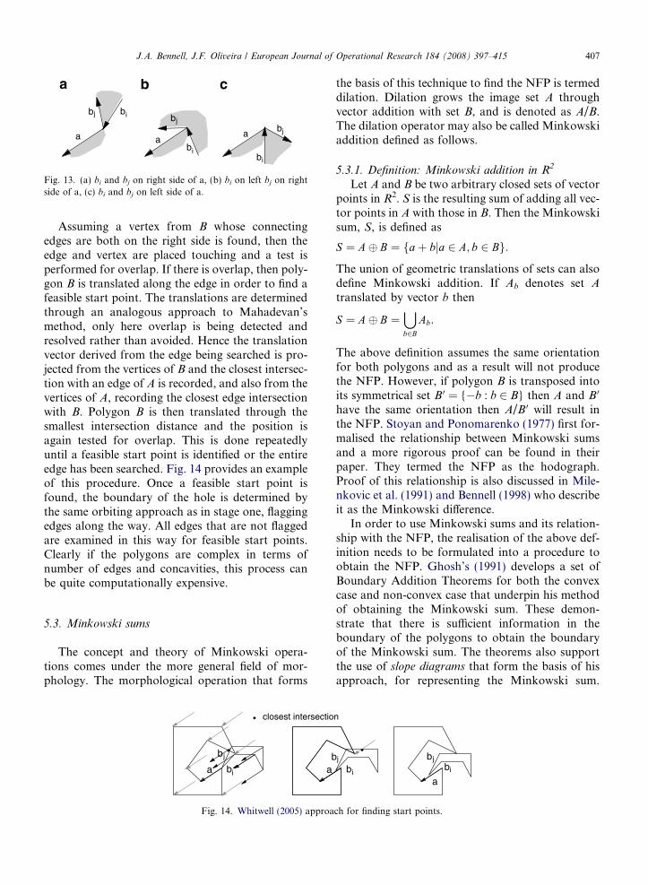
This approach as described by Mahadevan(1984) only holds for pairs of polygons that are rel-atively simply connected polygons. The outerboundary of the NFP can be found for instancessuch as that illustrated in Fig. 10, but not the holesor points of fit. Whitwell (2005) extended Maha-devan’s approach in order to address this drawback.The basic premise is that, if an edge of a polygonhas not been traversed when executing Mahad-evan’s approach then these edges potentially repre-sent a hole. If a feasible starting point for thesliding algorithm can be found on the unvisitededges then the equivalent sliding operation, inclockwise direction, can be performed to find theboundary of the hole (or inner-fit polygon).

The first step of Whitewell’s orbiting approachessentially follows that of Mahadevan with a modi-fied implementation to speed up the edge-pair detec-tion process. In addition, any edge traversed duringthis process is flagged. Edges of A and B that are notflagged are then evaluated in the second stage forfeasible starting points. There are two elements tothis procedure, first is to find an edge-vertex pairthat could potentially yield a valid start point, thesecond is to find a valid start point along the edge.

All edges that are not flagged are considered.Given there is an edge from A that is not flagged,then the vertices from B that can slide along thatedge are identified by evaluating whether the edgesthat connect at that vertex are both on the right side

of the edge of A. If they are both on the left side orone of the left and one on the right, there is no pos-sibility for feasible sliding between the edge and thatvertex. Fig. 13 illustrates this.

bibi

bi

bj

bj bj

aaa

Fig. 13. (a) bi and bj on right side of a, (b) bi on left bj on rightside of a, (c) bi and bj on left side of a.


Assuming a vertex from B whose connectingedges are both on the right side is found, then theedge and vertex are placed touching and a test isperformed for overlap. If there is overlap, then poly-gon B is translated along the edge in order to find afeasible start point. The translations are determinedthrough an analogous approach to Mahadevan’smethod, only here overlap is being detected andresolved rather than avoided. Hence the translationvector derived from the edge being searched is pro-jected from the vertices of B and the closest intersec-tion with an edge of A is recorded, and also from thevertices of A, recording the closest edge intersectionwith B. Polygon B is then translated through thesmallest intersection distance and the position isagain tested for overlap. This is done repeatedlyuntil a feasible start point is identified or the entireedge has been searched. Fig. 14 provides an exampleof this procedure. Once a feasible start point isfound, the boundary of the hole is determined bythe same orbiting approach as in stage one, flaggingedges along the way. All edges that are not flaggedare examined in this way for feasible start points.Clearly if the polygons are complex in terms ofnumber of edges and concavities, this process canbe quite computationally expensive.

5.3. Minkowski sums

The concept and theory of Minkowski opera-tions comes under the more general field of mor-phology. The morphological operation that forms

closest intersectio

bi

bj

ab

a

Fig. 14. Whitwell (2005) approa

the basis of this technique to find the NFP is termeddilation. Dilation grows the image set A throughvector addition with set B, and is denoted as A/B.The dilation operator may also be called Minkowskiaddition defined as follows.

5.3.1. Definition: Minkowski addition in R2

Let A and B be two arbitrary closed sets of vectorpoints in R2. S is the resulting sum of adding all vec-tor points in A with those in B. Then the Minkowskisum, S, is defined as

S ¼ A� B ¼ faþ bja 2 A; b 2 Bg:

The union of geometric translations of sets can alsodefine Minkowski addition. If Ab denotes set A

translated by vector b then

S ¼ A� B ¼[b2B

Ab:

The above definition assumes the same orientationfor both polygons and as a result will not producethe NFP. However, if polygon B is transposed intoits symmetrical set B 0 = {�b : b 2 B} then A and B 0

have the same orientation then A/B 0 will result inthe NFP. Stoyan and Ponomarenko (1977) first for-malised the relationship between Minkowski sumsand a more rigorous proof can be found in theirpaper. They termed the NFP as the hodograph.Proof of this relationship is also discussed in Mile-nkovic et al. (1991) and Bennell (1998) who describeit as the Minkowski difference.

In order to use Minkowski sums and its relation-ship with the NFP, the realisation of the above def-inition needs to be formulated into a procedure toobtain the NFP. Ghosh’s (1991) develops a set ofBoundary Addition Theorems for both the convexcase and non-convex case that underpin his methodof obtaining the Minkowski sum. These demon-strate that there is sufficient information in theboundary of the polygons to obtain the boundaryof the Minkowski sum. The theorems also supportthe use of slope diagrams that form the basis of hisapproach, for representing the Minkowski sum.

bi

bj

a

n

bi

j

ch for finding start points.


See Ghosh (1991) for a detailed explanation of thesetheorems and Bennell (1998) for a discussion of theapproach with respect to the NFP.

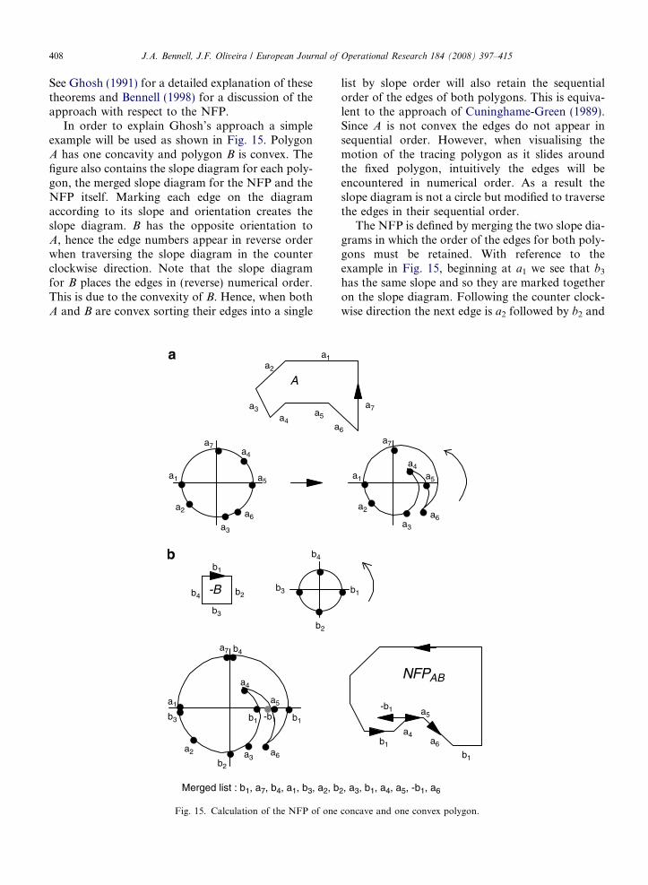
In order to explain Ghosh’s approach a simpleexample will be used as shown in Fig. 15. PolygonA has one concavity and polygon B is convex. Thefigure also contains the slope diagram for each poly-gon, the merged slope diagram for the NFP and theNFP itself. Marking each edge on the diagramaccording to its slope and orientation creates theslope diagram. B has the opposite orientation toA, hence the edge numbers appear in reverse orderwhen traversing the slope diagram in the counterclockwise direction. Note that the slope diagramfor B places the edges in (reverse) numerical order.This is due to the convexity of B. Hence, when bothA and B are convex sorting their edges into a single

a1

a3a4

a5

a

a2

a2

a1

a7

a3

a4

a6

a5

b2b4

b3

b1

a2 a3

a7

a1

b1 -b1

b2

b3

b4

b4

b1

a6

a4

a5

Merged list : b1, a7, b4, a1, b3, a2, b

A

-B b3

b2

Fig. 15. Calculation of the NFP of one

list by slope order will also retain the sequentialorder of the edges of both polygons. This is equiva-lent to the approach of Cuninghame-Green (1989).Since A is not convex the edges do not appear insequential order. However, when visualising themotion of the tracing polygon as it slides aroundthe fixed polygon, intuitively the edges will beencountered in numerical order. As a result theslope diagram is not a circle but modified to traversethe edges in their sequential order.

The NFP is defined by merging the two slope dia-grams in which the order of the edges for both poly-gons must be retained. With reference to theexample in Fig. 15, beginning at a1 we see that b3

has the same slope and so they are marked togetheron the slope diagram. Following the counter clock-wise direction the next edge is a2 followed by b2 and

a2

a4

a5

a3

a6

a7

a1

6

a7

b1

a4

a5

a6

-b1

b1

2, a3, b1, a4, a5, -b1, a6

NFPAB

b1

concave and one convex polygon.


a3. Next a5 is encountered but cannot be includedbefore a4. Therefore the traversal goes straight toa4 passing and including b1 along the way and thenreturns to a5 and on to a6. However, in order to getfrom a4 to a5 to a6 b1 is passed a second time in theopposite direction and so b1 is included again butwith a negative sign. Finally b1 is included a thirdtime on the traversal between a6 and a7 and b4.The resulting NFP and final merged list is detailedat the bottom of Fig. 15. Note that for each polygonthe edges retain their sequential order wherechanges in direction are permitted. The resultingNFP is not a simple polygon but has some internaledges or loops. This is an inevitable result of theboundary addition theorem and is explained inmore detail in Ghosh (1991). These loops need tobe examined with respect to their orientation as theymay represent holes in a multiply connected poly-gon. This is dealt with by Ramkumar (1996), Ben-nell (1998) and Bennell and Song (2005).

The above method can be extended to the casewhere neither polygon is convex, provided the con-cavities do not interfere with one another. If, how-ever two concavities interact then there will beareas of the slope diagram where both sets of edgesare not in sequential ordered. Ghosh (1991) dealswith this by splitting the slope diagram into parallelpaths, one for each concavity that interacts, whereeach path through the slope diagram defines a poly-gon. The NFP is the union or outer face of thesepolygons. Although the theory of traversal by paral-lel paths holds true, there are considerable imple-mentation problems in sorting out paths withmore complex instances.

Bennell et al. (2001) propose an approach thatextracts key elements of Ghosh’s approach anddevelops a set of algorithmic steps that produce asingle path through the slope diagram to producethe NFP. Their approach is based on the observa-tion that the simple-convex case can easily be dealtwith by Ghosh’s approach. As a result, theirapproach first replaces B by its convex hull, denotedas conv(B), and solves the simpler case of findingthe NFP of a simple and convex polygon, denotedas NFPAconv(B). To obtain NFPAB the convex edgesthat replaced the concavity in the convex hull aresubstituted with the original edges from the concav-ity plus any A edges that are traversed whereverthey appeared on the slope diagram.

Bennell and Song (2005) illustrate some draw-backs of the Bennell et al. (2001) algorithm, andpresent some modifications to provide a more

robust approach. Instead of generating the convexhull and then repairing the resulting NFP, they pro-pose an approach that retains the concavities of thepolygons but partitions one of the polygons intogroups of sequential edges according to whetherthey are convex or concave. Each of the groupscan then be individually merged with the slope dia-gram of A without conflict and then linked. Sincethe groups are not a complete cycle, the startingedge must be the first B edge in the group. Giventhe groups will be linked, it is necessary to finish agroup moving forward in a counter clockwise direc-tion, equivalent to a positive B edge. Since B edgesmay appear more than once, the leading B edgemust be positive and result in its final appearancealso being positive (e.g. +bi, �bi, +bi). When com-bining the merged lists, linking edges need to beincluded in order to maintain the precedence orderof the edges in each polygon.

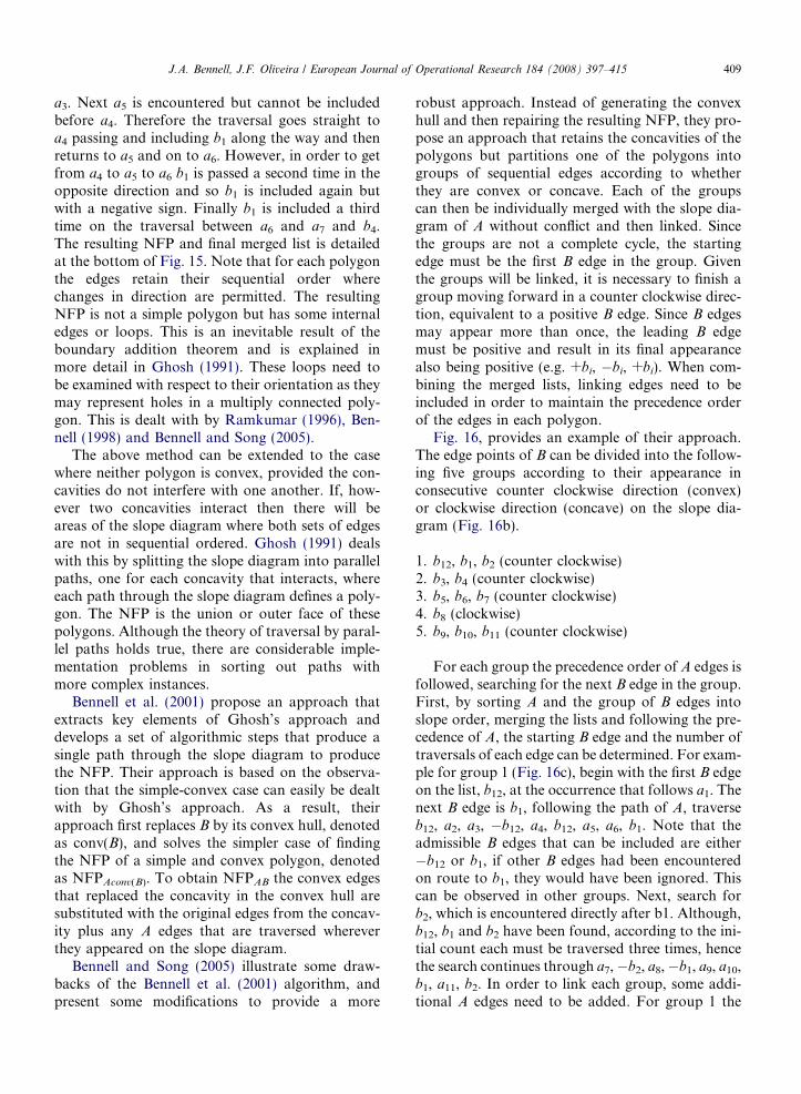
Fig. 16, provides an example of their approach.The edge points of B can be divided into the follow-ing five groups according to their appearance inconsecutive counter clockwise direction (convex)or clockwise direction (concave) on the slope dia-gram (Fig. 16b).

1. b12, b1, b2 (counter clockwise)2. b3, b4 (counter clockwise)3. b5, b6, b7 (counter clockwise)4. b8 (clockwise)5. b9, b10, b11 (counter clockwise)

For each group the precedence order of A edges isfollowed, searching for the next B edge in the group.First, by sorting A and the group of B edges intoslope order, merging the lists and following the pre-cedence of A, the starting B edge and the number oftraversals of each edge can be determined. For exam-ple for group 1 (Fig. 16c), begin with the first B edgeon the list, b12, at the occurrence that follows a1. Thenext B edge is b1, following the path of A, traverseb12, a2, a3, �b12, a4, b12, a5, a6, b1. Note that theadmissible B edges that can be included are either�b12 or b1, if other B edges had been encounteredon route to b1, they would have been ignored. Thiscan be observed in other groups. Next, search forb2, which is encountered directly after b1. Although,b12, b1 and b2 have been found, according to the ini-tial count each must be traversed three times, hencethe search continues through a7,�b2, a8,�b1, a9, a10,b1, a11, b2. In order to link each group, some addi-tional A edges need to be added. For group 1 the

a2

a3

b2

a5

a7a8

a10

a11

b12

b2

b4

b8b10

b12

b1

b1

b3

b6

b9

b11

a1

a4

a6

a9

a12

a4

a6a9

a12

a1

b7

b3

b6

b11

b9

b1

b5

a2

a3

a5

a7a8

a10

a11a4

a6a9

a12

a1

-b12

Fig. 16. Example to illustrate Bennell and Song (2005) approach.


final A edge is a12 and the first A edge in group 2 is a7,hence the path returns through �a12 to �a7 to retainthe precedence order. The full edge list is detailedbelow, where the A edge that precedes the startingB edge is included in square brackets to indicatethe starting point, but is not part of the edge list.The linking edges are underlined.

1. [a1], b12, a2, a3, �b12, a4, b12, a5, b1, a6, b2, a7, �b2,a8, �b1, a9, a10, b1, a11, b2, �a11, �a10, �a9, �a7

2. [a6], b3, b4, a7, �b4, a8, �b3, a9, a10, a11, b3, b4,�a11, �a10, �a9, �a7

3. [a6], b5, a7, �b5, a8, a9, a10, a11, b5, a12, b6, a1, b7,a2, �b7, a3, �b6, a4, b6, a5, b7, a6, a7, a8, a9, �b7,a10, b7, �a10, �a9, �a7, �a6, �a5

4. [�a5], b8, �a4, �b8, �a3, �a2, b8, a2, a3, a4, a5

5. [a6], b9, a7, �b9, a8, a9, a10, a11, b9, a12, b10, a1, b11,a2, �b11, a3, �b10, a4, b10, a5, b11, a6, a7, a8, a9,�b11, a10, b11, �a10, �a9, �a7, �a6, �a5, �a4,�a3, �a2

The resulting Minkowski sum is a complex (selfcrossing) polygon where the edges include all theedges of the NFP and some internal points. Theedges that are internal need to be removed. Note thatthis procedure will find holes and exact fit, as illus-trated in Fig. 10, as well as the boundary. Bennelland Song (2005) explain that the negative edgesand linking edges cannot be part of the boundaryof the NFP and can be removed. As a result the


sequence of edges is broken up into polygonal

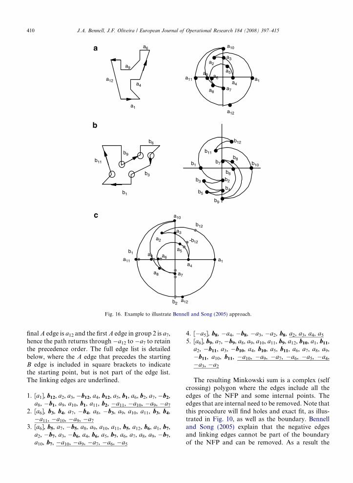
trips.The next step identities all the intersection points

between the polygonal trips, and flags them with a‘�’, indicating it is entering the trip, or with a ‘+’,indicating it is leaving the trip. Consider the examplein Fig. 17a, where the current trip is trip 2. Imaginestanding at the beginning of the first edge of trip 2facing along the edge, then consider that trip 1 inter-sects trip 2 from right to left. Trip 1 is said to enter

trip 2 and is marked with ‘�’. Continuing along trip2, eventually intersection with trip 4 is found, wheretrip 4 intersects from left to right. Trip 4 is leaving

trip 2 and marked with ‘+’. Hence, entering a tripmeans the beginning part of the intersecting edgeis on the right side of the trip edge and leaving cor-responds to the beginning part of the intersectingedge is on the left side of the trip edge. The frag-ments of trips that span a ‘�’ intersection to a ‘+’intersection are kept to form the boundary of theNFP. All other fragments are discarded.

3

2

4

1

-

+

-+

2

4

1+

Fig. 17. Procedure for removing internal edges from the Minkowski s(b) truncate each trip retaining parts between ‘�’ and ‘+’, (c) repeat an

x

x

B

A

x


Roo

Origin of Aand NFP

a1

a1

a

B

A

Fig. 18. Different origins of the same NFP

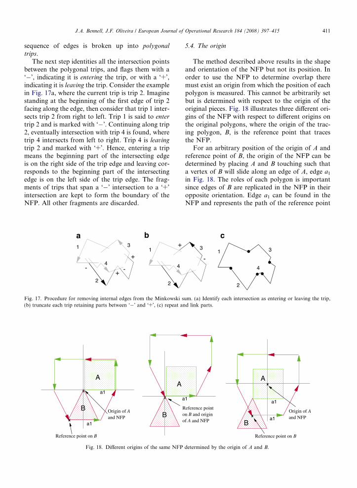
5.4. The origin

The method described above results in the shapeand orientation of the NFP but not its position. Inorder to use the NFP to determine overlap theremust exist an origin from which the position of eachpolygon is measured. This cannot be arbitrarily setbut is determined with respect to the origin of theoriginal pieces. Fig. 18 illustrates three different ori-gins of the NFP with respect to different origins onthe original polygons, where the origin of the trac-ing polygon, B, is the reference point that tracesthe NFP.

For an arbitrary position of the origin of A andreference point of B, the origin of the NFP can bedetermined by placing A and B touching such thata vertex of B will slide along an edge of A, edge a1

in Fig. 18. The roles of each polygon is importantsince edges of B are replicated in the NFP in theiropposite orientation. Edge a1 can be found in theNFP and represents the path of the reference point

3

-3

2

4

1

um. (a) Identify each intersection as entering or leaving the trip,d link parts.

x

xOrigin of Aand NFP


eference pointn B and origin f A and NFP

1a1

a1B

A

determined by the origin of A and B.

(0,0)

(1,1)

(1,0) (0,0)

A1

B2B1

A2

p

q

r

o

NFPA1B1NFPA2B2NFPA2B1NFPA1B2

o

p

q

r

NFPAB

Fig. 19. Calculation of the NFP using convex decomposition.


as B slides along edge a1. By positioning A and B

touching at the start of a1 and aligning the start ofa1 in the NFP at the reference point of B, the originof the NFP is given by the origin of A.

In the case of assigning the bottom left corner ofthe enclosing rectangle of both component polygonsas the origin, then the origin of the NFP is found atthe top right corner of the enclosing rectangle of thetracing polygon if it is placed at the bottom left cor-ner of the enclosing rectangle of the NFP. The theorythat underpins this can be found in Bennell (1998).

5.5. Decomposition

Given the complexity of obtaining the NFP whenconcavities between polygons interact, an alterna-tive approach is to decompose them into a numberof more manageable shapes. Watson and Tobias(1999) and Agarwal et al. (2002) decompose simplepolygons into convex sub-polygons. As described byCuninghame-Green (1989) the NFP of two convexpolygons can be calculated quickly and easily andis also a convex polygon. Li and Milenkovic(1995) decompose into star shaped polygons. A starshaped polygon is one that contains at least onepoint, called the kernel, such that a line drawnbetween that point and any point on the boundaryis wholly contained within the polygon. Li andMilenkovic show that the Minkowski difference oftwo star shaped polygons is also a star shaped poly-gon. Both decomposition methods are attractive asthey remove the requirement of detecting holeswhen calculating the NFP of each pair of decom-posed parts of the polygons. Here we will focus onconvex decomposition.

The principle of these approaches is to decom-pose each polygon into convex sub-polygons, gener-ate the NFP of each pair of sub-polygons where themembers of the pair arises from different polygons,and finally combine the NFPs of the sub-polygonsto generate the NFP of the two original polygons.The approach can be illustrated by consideringWatson and Tobias (1999). They decompose a sim-ple polygon into a set of convex polygons by cuttingbetween pairs of concave vertices. If there are anodd number of concave vertices then the last cut isbetween a concave and a convex vertex. The NFPof each sub-polygon can be found by the simpleedge sorting procedure described earlier in thepaper. The final step is to combine the sub-NFPsinto one polygon. Such a procedure requires theidentification of all edge intersections, since these

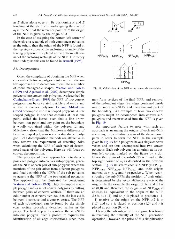
may form vertices of the final NFP, and removalof the redundant edges (i.e. edges contained insideone or more sub-NFPs and therefore not part ofthe boundary). An example of how two concavepolygons might be decomposed into convex sub-polygons and reconstructed into the NFP is givenin Fig. 19.

An important feature to note with such anapproach is arranging the origins of each sub-NFPaccording to the relative origins of the decomposedparts in order to form the NFP. In the examplegiven in Fig. 19 both polygons have a single concavevertex and are thus decomposed into two convexpolygons. Each sub polygon has an origin at its bot-tom left corner, marked on the figure by a dot.Hence the origin of the sub-NFPs is found at thetop right corner of Bi as described in the previoussection. Fig. 19 illustrates each sub-NFP (NFPA1B1,NFPA1B2, NFPA2B1, NFPA2B2) and their originsmarked as o, p, q and r respectively. When recon-structing the sub-NFPs the position of their originis determined by the vector difference a � b of theorigins. In the example the origin of A1 and B1 isat (0, 0) and therefore the origin o of NFPA1B1 isat (0,0) i.e. equivalent to the origin of the NFP.B2 is at (1,1) and so p is placed at position (�1,�1) relative to the origin on the NFP. A2 is at(1,0) and so q is placed at position (1,0) and r isplaced at position (0, �1).

Clearly the advantage of this approach is foundin removing the difficulty of the NFP generationoperation. However, the price of this simplification


is the complexity of the decomposition and combin-ing phases. Also, the effectiveness of the decomposi-tion phase has a direct effect on the efficiency of thecombining phase. For example, if A is decomposedinto p sub-polygons and B decomposed into q sub-polygons then p · q sub-NFPs need to be foundand assembled in the correct way to form NFPAB.It stands to reason that the fewer sub-polygonsrequired to decompose the polygon, the fewer sub-NFPs are generated and as a result the fewer edgesneed to be analysed for intersection and inclusion inthe combining process. However, decomposing apolygon in to the minimum number of convex poly-gons is significantly more computationally expen-sive than greedy methods. Agarwal et al. (2002)evaluate this issue further by experimenting with arange of different decomposition methods includingtriangulations, optimal decomposition and heuris-tics, in order to examine the effect on computationaltime. They found that although optimal decomposi-tion in general significantly reduces the computationtime for the Minkowski sum construction, thedecomposition is computationally expensive andheuristics that approximate optimal decompositionare preferred. In addition they discovered that therelationship between the number of convex sub-polygons and the time to construct the final NFPwas not a straight forward trade-off. Experimenta-tion demonstrated that the relationship betweenthe two polygons to be summed impacts on theMinkowski sum construction. Hence, they decom-pose the polygons simultaneously in order to mini-mise a cost function that takes account of thisrelationship. Other issues that arise from the con-struction phase are the identification of degeneratecases as illustrated in Fig. 10b and c. Case 10bwould be represented by co-linear edges not con-tained in any sub-NFP, and 10c would be foundat an intersection point of more than two edgesnot contained in any sub-NFP. These instanceswould all need to be tested directly.

5.5.1. Summary

The NFP is an efficient tool for detecting the rel-ative position between pieces. However, calculatingthe NFP is a non-trivial task and software to do thisis not publicly available. Hence many researchers donot exploit the benefits of the NFP due to the signif-icant investment in developing the tools required. Inaddition all the approaches above have their limita-tions. Mahadevan’s approach can not identify nest-ing positions that would result in a multiply

connected NFP; Ghosh’s approach overcomes thisbut can become complex resulting in many internalloops. In addition, instances where one piece fitsexactly into a nested concavity would be definedas a point or line within the NFP. Mechanisms toidentify the orientation of this type of ‘‘loop’’ lar-gely resort to direct testing (Bennell and Song,2005; Whitwell, 2005).

6. Phi function

The phi-function is the most recent innovation indealing with the geometric issues for nesting prob-lems. Its purpose is to represent all mutual positionsof two objects (in this context polygons), and there-fore it is often associated with the NFP. However,this association is misleading as the NFP is only aspecial case of the broader theory. The Phi-functionfor cutting and packing were conceived and appliedby Stoyan et al. (2001, 2004) and this research groupcontinue to be the main users of this methodology.The lack of an algorithmic process for generatingthe phi-function for arbitrary shapes may explainwhy this approach has not been more broadlyadopted. However, the phi-function is a powerfultool that warrants further research in order to facil-itate its use in the wider research community. In thissection we will simply illustrate the concept and itsapplication. See the original papers for detailed der-ivation of the mathematical functions.

The phi-function is a mathematical expressionsthat represent the mutual positions of two objects.Specifically the value of the phi-function is greaterthan zero if the objects are separated, equal to zeroif their boundaries touch and less than zero if theyoverlap. When the phi-function is normalised itsvalue is the Euclidean distance between the twoobjects, otherwise it is an estimate of the distance.Stoyan et al. derive the phi-function for primaryobjects; these are circles, rectangles, regular poly-gons, convex polygons and the compliment of theseshapes. Shapes that are not primary objects can berepresented as a union or intersection of the primaryobjects. Note that this is not decomposition sinceoverlap of primary objects is permitted. Hence wewill focus here on the phi-function for primaryobjects. The derivation of the functions is basedon trigonometry, and as far as we are aware, theyare derived by hand.

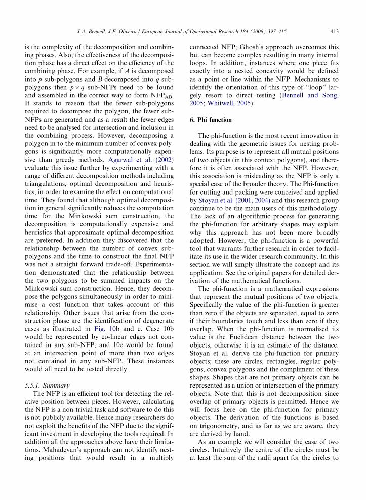
As an example we will consider the case of twocircles. Intuitively the centre of the circles must beat least the sum of the radii apart for the circles to

r1

22 r2r1yx +=+

r2

r1

+=+

Fig. 20. Representation of all touching positions of two circles.

y

Φ(x,y)=0

x

Φ(x,y)

Fig. 21. Plot of the phi-function for two circles.

•

•

•

Φ(x,y) = 0

Φ(x,y) > 0

•

•

•

•

••

•

Φ(x,y) = 0

Fig. 22. Two instances of the Phi-function.


not overlap. This is illustrated in Fig. 20 where circle1 as radius r1 and circle 2 has radius r2. Assumingcircle 1 is fixed at co-ordinate position (0,0), theequation

ffiffiffiffiffiffiffiffiffiffiffiffiffiffix2 þ y2

p¼ r1 þ r2 describes all the co-

ordinate positions of circle 2 (x,y) such that thetwo circles touch but do not overlap. Clearly if thecircles were separated then

ffiffiffiffiffiffiffiffiffiffiffiffiffiffix2 þ y2

p> r1 þ r2, and

the difference would be the Euclidean distancebetween the circles. Hence the phi-function canbe directly stated as: Uðx;yÞ¼

ffiffiffiffiffiffiffiffiffiffiffiffiffix2þ y2

p�ðr1þ r2Þ.

Finally if we remove the assumption that circle 1is fixed at (0,0) but instead is placed at co-ordinatepoint (x1, y1) and circle 2 is placed at co-ordinatepoint (x2,y2), then we need to translate both circlesthrough (�x1, �y1) so that circle 1 is again at theorigin and circle 2 has the equivalent relative posi-tion to circle 1. Therefore we can state the phi-func-tion for two circles at arbitrary positions as follows:

Uðx1;y1;x2;y2Þ¼ffiffiffiffiffiffiffiffiffiffiffiffiffiffiffiffiffiffiffiffiffiffiffiffiffiffiffiffiffiffiffiffiffiffiffiffiffiffiffiffiffiffiðx2� x1Þ2þðy2� y1Þ

2q

�ðr1þ r2Þ

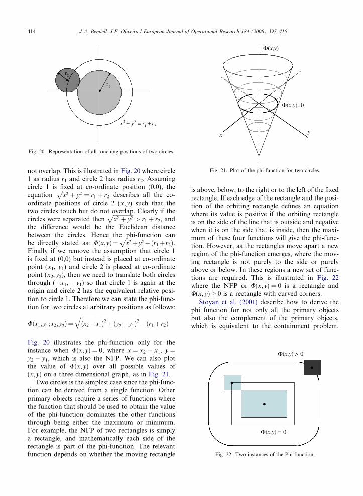
Fig. 20 illustrates the phi-function only for theinstance when U(x,y) = 0, where x = x2 � x1, y =y2 � y1, which is also the NFP. We can also plotthe value of U(x,y) over all possible values of(x,y) on a three dimensional graph, as in Fig. 21.

Two circles is the simplest case since the phi-func-tion can be derived from a single function. Otherprimary objects require a series of functions wherethe function that should be used to obtain the valueof the phi-function dominates the other functionsthrough being either the maximum or minimum.For example, the NFP of two rectangles is simplya rectangle, and mathematically each side of therectangle is part of the phi-function. The relevantfunction depends on whether the moving rectangle

is above, below, to the right or to the left of the fixedrectangle. If each edge of the rectangle and the posi-tion of the orbiting rectangle defines an equationwhere its value is positive if the orbiting rectangleis on the side of the line that is outside and negativewhen it is on the side that is inside, then the maxi-mum of these four functions will give the phi-func-tion. However, as the rectangles move apart a newregion of the phi-function emerges, where the mov-ing rectangle is not purely to the side or purelyabove or below. In these regions a new set of func-tions are required. This is illustrated in Fig. 22where the NFP or U(x,y) = 0 is a rectangle andU(x,y) > 0 is a rectangle with curved corners.

Stoyan et al. (2001) describe how to derive thephi function for not only all the primary objectsbut also the complement of the primary objects,which is equivalent to the containment problem.


This concept appears to have great potential forcontributing to the advancement of the field of nest-ing problems. However, the process of obtaining thephi-function has thus far acted as a barrier to wideradoption of this approach.

7. Conclusion

The paper has given a detailed description of theoperations of a number of different approaches fordealing with the geometry required in the solutionof nesting problems, these are; the raster method,direct trigonometry, the Nofit polygon and phi-functions. Each has its advantages and limitationsand a common theme is that the more computation-ally efficient the approach the more complex it is torealise. There is no doubt that there is a significantinvestment required in order to develop the geomet-ric tools necessary for tackling nesting problems.However, we hope that through this paper someof the mystery of these approaches has been dis-pelled and researchers are able to make an informedchoice when selecting their methodology.

Acknowledgement

The authors would like to sincerely thank Dr.Kathryn Dowsland for reviewing this manuscriptand providing valuable feedback.

References

Agarwal, P.K., Flato, E., Halperin, D., 2002. Polygondecomposition for efficient construction of Minkowskisums. Computational Geometry Theory and Applications 21,29–61.

Babu, A.R., Babu, N.R., 2001. A generic approach for nesting of2-D parts in 2-D sheets using genetic and heuristic algorithms.Computer-Aided Design 33, 879–891.

Beasley, J.E., 1985. Bounds for 2-dimensional cutting. Journal ofthe Operational Research Society 36, 71–74.

Bennell, J.A., 1998. Incorporating problem specific knowledgeinto a local search framework for the irregular shape packingproblem, PhD thesis, University of Wales, UK.

Bennell, J.A., Song, X., 2005. A comprehensive and robustprocedure for obtaining the nofit polygon using Minkowskisums, Working paper series, Centre for Operational Research,Management Science and Information Systems, University ofSouthampton, UK.

Bennell, J.A., Dowsland, K.A., Dowsland, W.B., 2001. Theirregular cutting-stock problem – a new procedure forderiving the no-fit polygon. Computers and OperationsResearch 28, 271–287.

Cuninghame-Green, R., 1989. Geometry, shoemaking and themilk tray problem. New Scientist 1677 (12 August), 50–53.

Dyckhoff, H., 1990. A typology of cutting and packing problems.European Journal of Operational Research 44, 145–159.

Ferreira, J.C., Alves, J.C., Albuquerque, C., Oliveira, J.F.,Ferreira, J.S., Matos, J.S., 1998, A Flexible Custom Com-puting Machine for Nesting Problems. In: Proceedings ofXIII DCIS, Madrid, Spain.

Ghosh, P.K., 1991. An algebra of polygons through the notion ofnegative shapes. CVGIP: Image Understanding 54 (1), 119–144.

Konopasek, M., 1981. Mathematical Treatments of SomeApparel Marking and Cutting Problems, U.S. Departmentof Commerce Report 99-26-90857-10.

Letchford, A.N., Amaral, A., 2001. Analysis of upper bounds forthe pallet loading problem. European Journal of OperationalResearch 132, 582–593.

Li, Z., Milenkovic, V., 1995. Compaction and separationalgorithms for non-convex polygons and their application.European Journal of Operations Research 84, 539–561.

Mahadevan, A., 1984. Optimisation in computer aided patternpacking, Ph.D. Thesis, North Carolina State University.

Milenkovic, V., Daniels, K., Li, Z., 1991. Automatic markermaking. In: Proceedings of the Third Canadian Conferenceon Computational Geometry, Simon Fraser University,Vancouver, BC, pp. 243–246.

Oliveira, J.F., Ferreira, J.S., 1993. Algorithms for nestingproblems, Applied Simulated Annealing. In: Vidal, R.V.V.(Ed.), Lecture Notes in Econ. and Maths Systems, Vol. 396.Springer Verlag, pp. 255–274.

Preparata, F.P., Shamos, M.I., 1985. Computational Geometry:An Introduction. Springer-Verlag.

Ramkumar, G.D., 1996. An algorithm to compute the Minkow-ski sum outer-face of two simple polygons. In: Proceedings ofthe 12th Annual Symposium on Computational GeometryFCRC 96.

Segenreich, S.A., Braga, L.M., 1986. Optimal nesting of generalplane figures: a Monte Carlo heuristical approach. Computers& Graphics 10, 229–237.

Stoyan, Y.G., Ponomarenko, L.D., 1977. Minkowski sum andhodograph of the dense placement vector function, Reports ofthe SSR Academy of Science, SER.A 10.

Stoyan, Y.G., Terno, J., Scheithauer, G., Gil, N., Romanova, T.,2001. Phi-functions for primary 2D-objects. Studia Inform-atica Universalis 2 (1), 1–32.

Stoyan, Y., Scheithauer, G., Gil, N., Romanova, T., 2004.U-functions for complex 2D-objects. 4OR: Quarterly Journalof the Belgian, French and Italian Operations ResearchSocieties 2, 69–84.

Watson, P.D., Tobias, A.M., 1999. An efficient algorithm for theregular W1 packing of polygons in the infinite plane. Journalof the Operational Research Society 50 (10), 1054–1062.

Waescher, G., Haussner, H., Schumann, H., 2005. An improvedtypology of cutting and packing problems, European Journalof Operations Research, forthcoming.

Whitwell, G., 2005. PhD. thesis, School of Computer Sciences,University of Nottingham, UK.

Y, G.G., Kang, M.K., 2002. A new upper bound for uncon-strained two-dimensional cutting and packing. Journal of theOperational Research Society 53 (5), 587–591.

Documents

The geometry of nesting problems: A tutorial - vmk.ugatu.ac.ruvmk.ugatu.ac.ru/c&p/article/new/nesting_problems_tutorialEJOR-184... · The geometry of nesting problems: A tutorial