The Geography of Unconventional Innovation

Enrico Berkes Ruben Gaetani∗

1st July 2016

Abstract

This paper studies the role of population density as a driver of innovation. Using a

newly assembled dataset of georeferenced U.S. patents, we show that overall innovation

activity is not concentrated in high-density areas as commonly believed. However, when

we restrict attention to unconventional innovations, that is innovations based on unusual

combinations of existing knowledge, we show that these are indeed more prevalent in

high-density areas. To interpret this relation, we propose, and provide evidence, that

informal interactions in densely populated areas help knowledge flows between distant

fields, but are less relevant for flows between close fields. We build a model of innova-

tion in a spatial economy that endogenously generates the pattern observed in the data:

specialized clusters emerge in low-density areas, whereas high-density cities diversify

and produce unconventional ideas.

JEL Classification: O33, O40, R11, R12

∗Northwestern University, Department of Economics. 2001 Sheridan Road, Evanston, IL, 60208. EnricoBerkes: enrico.berkes@u.northwestern.edu; Ruben Gaetani: gaetani@u.northwestern.edu. We thank for theircomments Treb Allen, David Berger, Lawrence Christiano, Matthias Doepke, Martin Eichenbaum, BenjaminJones, Lorenz Kueng, Matteo Li Bergolis, Lee Lockwood, Guido Lorenzoni, Kiminori Matsuyama, Nicola Per-sico, Giorgio Primiceri, Jorg Spenkuch and seminar participants at the 2015 Meeting of the Society for Eco-nomic Dynamics in Warsaw, 2015 World Congress of the Econometric Society in Montreal, Northwestern, OhioState University, Toulouse School of Economics, Collegio Carlo Alberto, University of Toronto, Chicago Fed,Atlanta Fed, Federal Reserve Board, 2014 Conference of Swiss Economists Abroad. Comments are welcome,errors are ours.

1 Introduction

The idea that informal interactions are central to innovation and knowledge diffusion hasbecome a cornerstone of recent theories of economic growth (Lucas 1988). If true, this ideaimplies that economic geography, by determining the extent of those interactions, shouldplay a first-order role in the creation and diffusion of knowledge. Specifically, we wouldexpect that innovation should cluster in high density areas, and that cities should be a keyengine of technological progress. There exists a sizeable literature on the role of cities andagglomeration for growth that builds on this intuition (Glaeser et al. 1992, Black and Hende-rson 1999, Glaeser 1999).

In this paper, we examine the link between density and innovation empirically, usingnarrowly georeferenced information on patenting in the United States. Our geographicallydisaggregated data show that the advantage of cities in producing innovation is more nu-anced than commonly believed. While suburban areas are responsible for a substantial shareof overall innovation activity, high-density places disproportionately generate innovationwith a high degree of unconventionality. This pattern, which to the best of our knowledgehas never been documented, reconciles the intuition that density fosters creativity with theobservation that the origin of innovation in the U.S. is not limited to dense urban areas. Wethen propose a spatial theory of a knowledge-based economy that is consistent with ourfindings. The theory highlights a novel rationale for why economic activity agglomeratesin cities of different sizes and degrees of diversification. This rationale is grounded in theprocess of knowledge creation and reconciles the tension between returns to local specializa-tion (Marshall 1890) and returns to diversity (Jacobs 1969), without relying on agents whoseproductivity is ex-ante heterogeneous. We use our model for policy analysis, and find thata system of place-based subsidies can have a significant impact on aggregate welfare bychanging both the intensity and composition of innovation activity.

We start by collecting the full-text record of all the patents granted by the USPTO in theyears 2002-2014, that we then georeference at the County Sub-Division (CSD, henceforth)level. This level of disaggregation allows us to capture previously disregarded variationwithin metropolitan areas or commuting zones. We document four novel facts on the spatialdistribution of innovation in the United States.

First, the role of high-density regions as engines of innovation is smaller than commonlythought. Over 40% of the patents in our sample originate from units with density of pop-ulation below 1, 000 people per square kilometer.1 Unsurprisingly, density is positively

1As reference points, the density of Manhattan in 2014 was 27, 000/km2, Chicago 4, 400/km2, Los Angeles3, 200/km2, Austin 1, 300/km2, Palo Alto 960/km2 and Armonk (NY) 280/km2.

1

related to innovativeness along the extensive margin: more densely populated places aremore likely to consistently host innovative activity. However, among continuously innovat-ive CSDs - defined as units that produced at least one patent per year - innovation intensity(measured as patents per capita) and population density display a weak, non-monotonicrelationship that is best described by an inverted-U curve. In particular, in dense locations,higher population density does not translate into higher rate of invention.

Second, innovation produced in densely populated areas is more likely to be built uponunconventional combinations of prior knowledge. To show this fact, we formulate a notionof technological distance that proxies for the intensity of idea flows between fields, based onthe observed network of patent citations. We develop an algorithm in the spirit of Uzzi etal. (2013) to evaluate the atypicality of references listed in each patent. Our measure com-pares the observed frequency of each pairwise combination of citations with the frequencyone would expect if references were distributed at random. This procedure defines an in-dex of conventionality (c-score) for each citation pair: combinations are unconventional iftheir empirical frequency is small compared to their random frequency. The c-score ranksinventions along a dimension that we argue to be economically meaningful: first, uncon-ventional patents are significantly more likely to be highly cited compared to conventionalones; second, unconventional patents are significantly less likely to be produced by large,publicly traded firms. We find that unconventional innovations tend to originate dispropor-tionately from densely populated areas. This relationship is statistically and economicallysignificant, emerges both in patent-level and CSD-level regressions and is robust to a widevariety of specifications.

Third, dense cities host a more diversified pool of learning opportunities. Computing thetechnological distance between two patents produced in each CSD, we show that pairwisecombinations of inventions in high-density CSDs are more technically distant than combin-ations in low-density ones. The implication of this fact is that inventors in dense cities willbe more likely to be exposed to ideas from backgrounds distant from their own.

Fourth, the local pool of ideas is a strong predictor of the combinations embedded innew inventions. In other words, inventors exhibit a positive bias toward drawing ideas outof a pool that is locally determined. As a descriptive finding, we observe that for 75% of theclass pairs, a patent that references both classes in a given pair (A,B) is disproportionatelymore likely to appear in CSDs with a higher share of patents of class A and B.2 To controlfor endogenous locational choice, we adopt a difference-in-difference strategy and look atthe evolution of patenting of pre-existing firms upon arrival in town of a company from a

2Specifically, we observe that for 75% of the class pairs, a patent that references both classes in the pair(A,B) is more likely to appear in CSDs with a higher share of patents of class A or B, and disproportionatelymore likely when the product of the two shares is high (i.e. the coefficient of the interaction is positive).

2

different sector. We find that the arrival of a firm significantly biases the citation behavior ofpre-existing entities toward the field of the arriving firm. To the best of our knowledge, thispaper is the first to provide direct evidence of inter-sectoral localized knowledge spilloversoperating through this channel.

The facts that we document suggest an alternative interpretation of how technologicalchange interacts with economic geography. Overall, suburban areas play a prominent rolein the innovation process: for example, big innovative companies such as IBM or Motorolatend to perform their research in large office parks located outside main city centers. Oneview is that these companies can organize knowledge flows efficiently within the organiz-ation, and do not need to rely on happenstance interactions in a dense environment. Bycontrast, informal interactions in dense and diversified areas may become important in gen-erating knowledge flows across technologically distant fields, since specialized formal net-works (e.g. firms, academic departments and research labs) may not efficiently internalizethem. As a result, innovations originating in high-density areas will be built upon moreuncommon combinations of prior knowledge.

This new set of observations calls for a reassessment of the theoretical link between geo-graphy and innovation. In particular, a spatial model of innovation should be able to ac-count for the simultaneous emergence of specialized clusters in suburban areas and diversi-fied hubs in urban centers, while taking the heterogeneity of innovation into account. In thesecond part of the paper, we propose such a model and use it to perform policy analysis.

In our setting, innovators are specialized in one of a finite set of scientific fields andchoose where to locate balancing rent considerations and innovation opportunities. Afterdeveloping an idea, innovators can either implement it through an established firm, whichkeeps the monopoly power over its specific product and increases productivity, or combinetheir idea with the knowledge of an inventor of a different field. The second option leads toan unconventional innovation: the inventor can start up a new company and gain leader-ship over an existing product line, replacing the previous monopolist. Innovators have anincentive to cluster with people of similar background to benefit from intra-field spilloversthat increase their ability to develop ideas. However, interactions with inventors from dif-ferent fields require informal channels and are subject to search frictions. Density reducesfrictions across fields but is ineffective in fostering spillovers within fields.

The model reproduces the geographical sorting of innovation activity observed in thedata. Conventional and unconventional ideas are complementary. This leads to the emer-gence of asymmetric sites, both in terms of density and specialization. Densely popu-lated sites diversify and generate unconventional innovation, whereas specialized clustersemerge in low-density areas and produce conventional ideas. The equilibrium implies that

3

geography, composition and intensity of the innovative activity are tightly related, and de-pend on the parameters of the model in an intuitive way.

This unexplored link opens up novel possibilities for welfare improving place-basedtransfers. We study optimal policy numerically by calibrating the model using US data.Unconventional ideas are found to be mostly driven by business stealing considerations, asthey bring about little technological improvement compared to conventional ones. How-ever, they act as creative destruction events and limit the monopoly power in the economy,which translates into an improved static allocation of labor across firms. The equilibriumconceals a set of externalities that make the outcome inefficient in several dimensions. Thewelfare analysis reveals that a planner would use place-based policies to increase urbaniz-ation and boost creative destruction, at the cost of lowering growth and increasing conges-tion. The optimal policy of a planner who has the ability to fully affect the urban structureleads to a welfare gain 2 to 3 times larger (in consumption equivalent units) than the one ofa planner who can only intervene by reallocating people within the existing urban structure.

This paper contributes to the empirical literature on the estimation of localized know-ledge spillovers and the study of their implication for innovation and growth. The import-ance of localization and geography for the spreading of knowledge, which dates back toMarshall (1890),3 has been the subject of extensive empirical study in recent years sinceLucas (1988), Krugman (1991) and Glaeser et al.’s (1992) seminal papers on economic de-velopment and economic geography. Jaffe et al. (1993) analyze the network of patents andfind that citation patterns display a significant bias towards patents that were producedin the same state and metropolitan area. Audretsch and Feldman (1996), Audretsch andStephan (1996) and Feldman and Audretsch (1999) analyze the geographical concentrationof production and innovation activities and find evidence of substantial complementaritiesbetween the two. Carlino et al. (2007) document a positive relationship between density andpatenting across MSAs. The urban literature has long been interested in the interaction ofknowledge spillovers with local specialization and diversity, as in Porter (1990), Florida andGates (2001), Delgado, Porter and Stern (2014). We contribute to this literature by explicitlyconsidering how local innovation activity affects the composition of the knowledge base uponwhich inventors build new ideas. Our analysis puts particular emphasis on inter-field tech-nology spillovers. Our main finding is broadly consistent with Packalen and Bhattacharya(2015), who find that over the last century newer concepts have been implemented in inven-

3In Marshall’s famous words: “When an industry has thus chosen a locality for itself, it is likely to stay therelong: so great are the advantages which people following the same skilled trade get from near neighborhoodto one another. The mysteries of the trade become no mysteries; but are as it were in the air, and children learnmany of them unconsciously.”

4

tions originating from high-density regions.4

This paper also contributes to the theoretical literature on spatial equilibria and know-ledge spillovers. Glaeser (1999) proposes one of the first models of knowledge flow in aspatial setting. The dichotomy between specialized and diversified sites in an innovationeconomy was first introduced by Duranton and Puga (2001). In their model, young firmslocate in diversified cities to experiment with different prototypes, while established firmsmove to specialized sites where intra-field spillovers are stronger. Davis and Dingel (2012)develop a model in which productivity in cities is fostered by informal interactions amongpeople living in a densely populated environment. In their setting, the spatial equilibriumis determined by the comparative advantage of high-skilled individuals in an environmentwith high learning opportunities. In our setting, individuals are homogeneous in all respectsexcept for the knowledge background they carry: density plays the peculiar role of favoringinteractions among people from different fields. As in Berliant and Fujita (2011), knowledgediversity is a key component of growth in our model.

Finally, this paper is related to the literature on endogenous growth and heterogeneousinnovation. Akcigit and Kerr (2010) develop a model with heterogeneous firms in the spiritof Klette and Kortum (2004) and explicitly allow for the possibility to carry out explora-tion R&D to acquire new product lines and exploitation R&D to improve existing ones. Weidentify exploration R&D with unconventional innovation. This choice is based on the em-pirical observation that unconventional patents have a substantially higher technologicalimpact than conventional ones. From a technical point of view, our model closely resemblesPeters (2013) and Hanley (2015) in assuming limit pricing and Cobb-Douglas final goodaggregator, allowing a simple decomposition of welfare into a static and a dynamic com-ponent. We innovate on the existing literature by integrating the idea of heterogeneousinnovation in a spatial equilibrium model of a system of cities.

The remainder of the paper is organized as follows: Section 2 introduces the datasetand presents four empirical facts on the geographical organization of innovation activityin the United States. Section 3 introduces the model, characterizes its solution, highlightsthe mechanism, performs the calibration and studies its implications. Section 4 analyzes

4Packalen and Bhattacharya (2015) find that throughout the last century, patents produced in more denselypopulated urban areas have made more intense use of newer concepts, identified as new sequences of words.On the contrary, we look directly at combinations of ideas. The pattern of geographical sorting that we docu-ment runs through a specific channel, namely, a more hybridized composition of the knowledge base uponwhich new ideas are built. Packalen and Bhattacharya (2015) also find that the advantage of dense cities issignificantly weaker in the part of the sample corresponding to the time period covered by this paper. Thissuggests that the sorting that we document could be even stronger if an earlier sample of patents were used.This is left for future research.

5

optimal place-based policies under fixed and flexible urban structure. Section 5 concludes.

2 Empirical Analysis

The analysis is performed using the universe of patents granted by the US Patent and Trade-mark Office (USPTO) between January 2002 and August 2014, and filed between January2000 and December 2010. Table B.1 reports the number of patents by filing year. There areseveral advantages to focusing on this recent sample. First, the recent digitization of thepatent archive has made it easier for authors and reviewers to look for earlier patents toreference. This is reflected in a significantly higher number of citations listed in each patent.Second, by focusing on a short period, we minimize long-run changes in the propensity topatent and the technological composition of the sample. Finally, by focusing on the 2000-2010 period, we can reliably link the location information in the patent with socio-economicand demographic characteristics from the Census and the American Community Survey.

Every patent is associated to one of 107 International Patent Classification (IPC) categor-ies.5 For each grant, we gather information on the identity and location of the originalassignee and the inventors and on the full list of referenced patents (up to a maximum of1,500 citations per patent). Every patent is geolocated following a hierarchical rule: If thepatent file reports the name of an institutional assignee (e.g. a company, a research lab or anacademic institution) we assign the patent to the geographical coordinates of their location;if the file does not report any assignee or its address is missing or located outside the UnitedStates, we attempt to geotag the grant according to the location of its first inventor, otherwiseof its second inventor and so on until we are able to assign a location to each patent.6 Weonly consider patents that reference at least two citations. The main analysis is performedon a final subset of 1,058,999 patents filed over an 11-year period.

5Since each grant is associated with several IPC classes but only one main USPTO class, we build a many-to-one function that maps every USPTO class to a single IPC class based on the association that recurs moreoften.

6Note that we choose to use the location of the assignee, whenever available, instead of the address of theinventor. Most of the literature on the subject, since Jaffe et al. (1993) uses the location of the inventor. Bothalternatives raise a number of issues. For example, when a patent lists multiple inventors whose locations aretoo far apart to suggest any interaction through spatial proximity, the address of the institution can representa more accurate indication of the geographical origin of the invention. Many companies issue patents underseveral addresses, corresponding to different establishments or research facilities. The main concern with ourapproach is that the address of the assignee sometimes represents the headquarters of the company insteadof the research facility. However, Aghion et al. (2015) report a 92% correlation between the two locations. Toaddress this concern, we run robustness checks using two separate geotagging strategies: (1) the sub sampleof patents assigned to the address of the firm, only when it is in the same state of the address of at least oneof the inventors and (2) all the patents located at the address of the inventor. We mention these checks severaltimes throughout the text.

6

The analysis is conducted at a County Sub-Division (CSD) level. The CSD represents thefinest geographical unit that we are able to identify uniquely by intersecting the location in-formation retrievable from the full-text of the patent and the data available from the Censusand the American Community Survey.7 The CSD is much finer than a county, it typicallycoincides with city boundaries and, in a few cases (e.g. New York City) a city can be par-titioned in multiple CSDs. Since demographic data at this level of disaggregation are onlyavailable every 10 years, we interpolate the values of the demographic variables between2000 and 2010 assuming a constant growth rate throughout the years.

2.1 Fact 1: The relationship between density of population and intensity

of patenting is non-monotonic

In our analysis, we are mostly concerned with characterizing patterns of innovation alongthe intensive margin. Namely, we restrict the focus to continuously innovative CSDs, definedas units that have filed at least one patent per year between 2000 and 2010. These areas ac-count for 53% of the U.S. population and 61% of college graduates in the 2010 U.S. laborforce. Roughly 95% of all the patents in our dataset originate from these units. Since we areinterested in measuring the extent to which density is related to the flow of knowledge, it isnatural to restrict the focus to areas that are continuously involved in innovation activities.The study of areas where innovation does not occur, or occurs only occasionally, is outsidethe scope of this paper.8

The map in Figure B.2 illustrates the distribution of continuously innovative locationsin the United States between 2000 and 2010 (see also Figure B.2 for close-up maps of thefour most densely populated metropolitan areas).9 There is a clear tendency for innovativeactivity to concentrate around main urban centers, highlighting a pattern that most wouldexpect. For example, the East-Coast, the Chicago Area, the Texas Triangle and the Bay Area,among others, are all highly innovative regions. However, two less obvious observationsalso emerge. First, a substantial part of patenting activity occurs away from main urbancenters, often in low-density areas that are geographically separated from major cities (not-ably, Armonk, NY and Schenectady, NY). Second, even within major urban agglomerations,a big share of the innovative action takes place in the suburban portion of the latter (e.g.Redmond, WA and Schaumburg, IL). Overall, low density regions seem to play a key rolein the innovation process. About 43.3% of the patents filed between 2000 and 2010 were

7The socio-economic and demographic indicators at the CSD level available at https://nhgis.org.8The model will assume complete separation between innovation and production locations.9Note that CSDs are a partition of the US: the empty areas are CSDs where no patents where filed between

2000 and 2010.

7

produced in CSDs with population density below 1,000 residents per square kilometer.10

2.1.1 Measurement

For most of the paper, the units of analysis correspond to CSD-year observations. We usepatents per resident as a proxy for innovation intensity (to test for robustness, we also usepatents per worker and patents per college-graduate). In the benchmark results, densityis measured as residents per square kilometer (or density of workers and density of col-lege graduates). We weight observations by total population (or total workers and totalnumber of college graduates) but similar patterns emerge if observations are unweighted orweighted by number of patents. We control for year fixed effects to account for aggregatetrends in density and patenting. Since the panel includes a high number of observations, weillustrate the results using bin-scatter plots: unless otherwise specified, we divide the vari-able on the x-axis in 20 bins - each containing the same weighted number of observations -and take the mean of the y-variable across the observations falling in each bin.11

2.1.2 Finding

In the cross-section, density is related to innovativeness on the extensive margin: increas-ing population density by 1% increases the probability of hosting permanent innovationactivities by 0.16% (Figure B.3a). As a result, the unconditional correlation between densityand patenting is positive and significant (Figure B.3b). However, this correlation is entirelydriven by very low-density places that have zero patenting. Plots B.3d-f show that the cor-relation is still positive across places with density above 100/km2 (d), but becomes flat whenwe condition on density being larger than 500/km2 (e) and even negative when we restrictour attention to places with density above 1, 000/km2 (f).

Figure 2.1 shows the relation between density and patenting along the intensive margin.In particular, it displays a bin-scatter plot of (log) population density and patents per personin the balanced panel of 1,645 continuously innovative CSDs.12 The relation appears to benon-monotonic, and best described by an inverted-U curve. A quadratic approximationyields a tipping point of roughly 980/km2, which corresponds approximately to the densityof Palo Alto (960/km2). In the portion of the sample that corresponds to dense urban centers,higher population density is not associated to a higher rate of invention.

10As a reference, the Census defines as urban those areas with a central block of at least 2, 500/km2, sur-rounded by blocks of at least 1, 300/km2.

11Chetty et al. (2013) show that this methodology graphically captures the correlation between two variables.See http://michaelstepner.com/binscatter/ for a discussion.

12The United States are partitioned into 35,612 CSDs, of which 10,907 patent at least once in the period

8

4 5 6 7 8 9 10Log density of population

0.0002

0.0004

0.0006

0.0008

0.0010

0.0012

Patents per ca

pita

Figure 2.1: Bin-scatter plot of patents per capita and (log) population density in continuously in-novative CSDs. The plot is weighted by total population and controls for year fixed effects. The lineis obtained through a quadratic interpolation.

Figure B.5 (left-panel) presents an alternative way of visualizing the relationship: werank CSDs according to their population density and plot the cumulative share of overallpatents (horizontal axis) and the cumulative share of overall population.13 As we wouldexpect in the absence of a monotonic relationship, the cumulative function largely overlapswith the 45-degree line.

2.1.3 Robustness

It is possible that the relationship observed in Figure 2.1 is distorted by the fact that con-tinuously innovative, skill-rich regions tend to be low-density (e.g. college or companytowns). In this case, we would be overestimating the relevant interaction opportunities indense cities and underestimating them for suburban areas. Panel (a) of Figure B.4 shows asimilar bin-scatter that captures the partial correlation between density and patenting percapita after controlling for the skill composition (namely, the percentage of college gradu-ates in the population). Panel (b) of the same Figure shows the unconditional correlation,

2000-2010. Within this subset, 95% of the patents originate from 1,645 continuously innovative CSDs.13The left-panel includes all the CSD-year observations. The right-panel shows the same exercise but drops

the observations corresponding to San Jose-Palo Alto.

9

but using density of college graduates and patent per college graduate instead.14 In bothspecifications, density and patenting display a clear inverted-U relationship.

The choice of a narrow geographical unit of analysis raises the possibility that commut-ing can confound local population density as a proxy for personal interactions. Also, thechoice of locating the address of the firm whenever possible raises the concern that a firmfiles the patent in a location that is different from the one of the research facility. To addressthis, we look at two extreme cases. In the first case, we assume that relevant interactionsonly occur at the workplace. We consider only the subset patents for which the assignee isin the same state of at least one of the inventors. In this case, we would be correctly assign-ing the location, but learning opportunities would be mismeasured, as density of workersshould be used instead of density of residents. Panel (c) of Figure B.4 shows the relationshipbetween density of workers and innovation intensity for this subset of patents. In the op-posite case, we assume that relevant interactions only take place at the inventor’s residence.This time, learning opportunities would be correctly measured by population density, butthe patents issued to institutional assignees would be wrongly geolocated. In Panel (d) ofFigure B.4, we plot the relationship by geolocating all the patents at the address of the firstinventor. In both polar cases, the same pattern of Figure 2.1 emerges.

By counting the raw number of patents we may be distorting the relationship betweendensity and innovation if inventors and firms locating in low-density places have a higherpropensity to issue low-quality patents, other things being equal. To address this possibility,we weight the number of patents issued by the number of future citations received. In Panel(e) of Figure B.4 we show the partial correlation of population density and citation-weightedpatents.15 We also run an additional test excluding Delaware and DC from the the sample,as those are classical examples of states for which the location of the assignee and of theinventor are more likely to differ.

2.2 Fact 2: Positive relationship between density and unconventionality

The intuition that learning opportunities offered by density should be strong enough to at-tract the bulk of innovation receives weak support from the data: suburban regions take ona relevant portion of aggregate patenting activity. Agglomeration positively correlates withthe rate of invention in low-density places, but not in high-density ones. A possible explan-ation is that density catalyzes the flow of knowledge across fields that are not connected

14In Panel (f) we plot the same relation, but dropping the observations corresponding to the state of Califor-nia.

15Although later patents have received on average a lower number of citations, year fixed effects accountfor this difference.

10

through established networks, whereas formal organizations are able to internalize know-ledge flows efficiently within their own field without relying on density-driven informalinteractions. As a result, higher density eventually does not translate into more intense pat-enting, but rather into a shift in the type of innovation produced.

In this subsection, we show that innovations produced in high-density areas tend to beconstructed on a more diversified set of prior knowledge. To assess this fact, we build anexact measure of hybridization of the knowledge base of each invention. We use the dis-tribution of citations across technological classes to infer the intensity of knowledge flowsbetween fields. The fact that a pair of patent classes is recurrently referenced together indic-ates frequent knowledge flows between the two. Conversely, the fact that the combinationof a given pair of categories is atypical denotes the lack of frequent knowledge transmissionbetween the two.

2.2.1 Measurement

We now describe how we measure the degree of interconnection between two technologicalclasses. We adapt the methodology proposed by Uzzi et al. (2013, UMSJ henceforth), whostudy atypical citation patterns in the universe of academic papers. To the best of our know-ledge, this paper is the first to apply a similar algorithm to patents. The basic idea is tocompare the frequency of a bundle of classes in the observed network of references with thefrequency one would obtain by assigning citations at random in a replicated network. Inthis process, the structure of the network is kept constant. In other words, the total numberof citations from class A to class B is the same in the two networks, but references in thereplicated network are reshuffled, so that the conditional correlation of referenced classeswithin a patent is zero.16 The conventionality-score (or c-score) of the pair (A, B) is thendefined as the ratio between the observed frequency and the random frequency:

c (A, B) = fobs (A, B)frand (A, B) .

16This is a departure from UMSJ that only keep the total number of citations from and into each class con-stant. We do this so that the c-score does not depend on the size of a given class relative to the whole sample.While aligning with the basic intuition in UMSJ, we differ from their implementation in two additional di-mensions. First, we do not consider the time dimension explicitly in the replicated network: the total numberof citations is kept constant across classes, but not across years. Given that our time window (2000-2010) isrelatively short, this simplification is not likely to have a big impact on our estimates. Second, we assumethat the number of nodes is big enough such that the law of large numbers applies, which allows us to havean analytical expression for the random frequency. This delivers an exact formula for the c-score, that can becomputed without simulating the replicas. For details on the computation procedure, see the discussion in theAppendix.

11

The interpretation of the c-score is straightforward: a high value of c means that we ob-serve classes A and B cited together relatively more often in the data than what we wouldexpect if citations were assigned pseudo-randomly. We refer to such a citation pair as “con-ventional” and infer that idea flows between A and B are relatively frequent. On the otherhand, a low ratio indicates that A and B are observed in the data relatively less often thanat random. In this case, the combination is defined as “unconventional”. For expositionalconvenience, in some cases we refer to u (A, B) = 1− c (A, B) as unconventionality-score(or u-score). The details of the algorithm are provided in Appendix.

Figure B.7 shows a heat-map of the symmetric c-score matrix: each pixel represents acitation pair and it is colored based on its c-score. For example, the pixels on the diagonalrepresent the score of citation pairs of the form (A, A). We use a chromatic scale in whichbrighter pixels denote more unconventional pairs. The figure highlights two patterns thatsupport the validity of the measure. First, combinations on the diagonal tend to be moreconventional than other citation pairs. This is exactly what we would expect: once a patentcites a certain class, it is likely that is going to cite the same class again, since that class islikely to play some role in the patent development. Second, around the diagonal we observesome “clusters” of conventionality. This happens because the IPC classification system tendsto assign close labels to classes that are technologically close. For example, classes in thetop-left cluster group all the patents related to human necessities. It is not surprising that acitation that falls in that group is likely to appear with another citation in the same group.17

We assign to each patent an entire distribution of c-scores, one for each pairwise com-bination of references (hence, a grant with N references is assigned (N

2 ) possibly identicalscores). Two statistics of the distribution are of particular interest. The 10th percentile (or“tail-conventionality”) proxies for the most unconventional pair of classes listed by the pat-ent.18 The median c-score (or “core-conventionality”) proxies for how tightly grounded thepatent is in prior knowledge. Figure B.6 plots the cdf of the core and tail-conventionality inour final sample. Consistently with the findings in UMSJ, it shows that the median patent ishighly conventional at the core (its core-conventionality is well above one).

Next, we show that having an unconventional tail is a powerful predictor of technolo-gical impact. To show this, in the spirit of UMSJ, we define a hit patent as an invention thatreceived more citations than 95% of the other grants issued in the same year and belonging

17However, the c-score identifies technological proximity also between classes that belong to different IPCclusters. The following are some significant examples: Food (belonging to the Human Necessities cluster) andSugar (belonging to the Chemistry cluster) have a c-score of 1.17; Butchery (Human Necessity) and Weapons(Metallurgy) have a c-score of 1.14; Decorative Arts (Printing) and Photography (Instruments) have a c-scoreof 1.15; Knitting (Textiles) and Brushware (Human Necessity) have a c-score of 1.84.

18In this paper we follow USMJ and use the 10th percentile for tail-conventionality, but our results are robustto using the minimum. We winsorize the c-score measure at the 1% level.

12

1 2 3 4Core Conventionality Category

0.035

0.040

0.045

0.050

0.055

0.060

0.065

0.070

Pr(Hit Patent)

Conventional TailUnconventional Tail

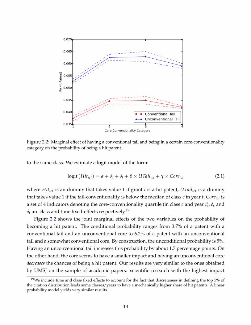
Figure 2.2: Marginal effect of having a conventional tail and being in a certain core-conventionalitycategory on the probability of being a hit patent.

to the same class. We estimate a logit model of the form:

logit (Hitict) = α + δc + δt + β×UTailict + γ× Coreict (2.1)

where Hitict is an dummy that takes value 1 if grant i is a hit patent, UTailict is a dummythat takes value 1 if the tail-conventionality is below the median of class c in year t, Coreict isa set of 4 indicators denoting the core-conventionality quartile (in class c and year t), δc andδt are class and time fixed-effects respectively.19

Figure 2.2 shows the joint marginal effects of the two variables on the probability ofbecoming a hit patent. The conditional probability ranges from 3.7% of a patent with aconventional tail and an unconventional core to 6.2% of a patent with an unconventionaltail and a somewhat conventional core. By construction, the unconditional probability is 5%.Having an unconventional tail increases this probability by about 1.7 percentage points. Onthe other hand, the core seems to have a smaller impact and having an unconventional coredecreases the chances of being a hit patent. Our results are very similar to the ones obtainedby UMSJ on the sample of academic papers: scientific research with the highest impact

19We include time and class fixed effects to account for the fact that discreteness in defining the top 5% ofthe citation distribution leads some classes/years to have a mechanically higher share of hit patents. A linearprobability model yields very similar results.

13

5 6 7 8 9Log density of population

0.19

0.20

0.21

0.22

0.23

0.24

0.25

Tail unco

nventionality

Figure 2.3: The dependent variable is defined as one minus the tail-conventionality of the medianpatent in the CSD-year observation. The bin-scatter plot is weighted by the total number of patentsfiled in the CSD/Year observation and controls for State and Year fixed effects.

appears strongly rooted in existing knowledge and at the same time displays the intrusionof novel combinations. This surprising similarity suggests that the process of innovation, nomatter if academic or applied, follows a somewhat universal pattern.20

The strong correlation between unconventionality and technological impact shows thatthe c-score is ranking patents along a meaningful dimension. Motivated by this result, inwhat follows we will use tail-conventionality as our reference measure.

2.2.2 Finding

One hypothesis is that density plays the decisive role of catalyzing knowledge diffusionacross unrelated fields. If this intuition is correct, we should observe that patents from high-density regions display more unconventional references. By facilitating interactions, densityallows people to gain insights they cannot acquire through their formal network. This trans-lates into new ideas obtained by assembling a more hybridized set of prior knowledge.

20The fact that high-impact research is novel and, at the same time, tightly grounded, is explained at leastin part by UMSJ by the necessity to efficiently deliver an idea to an inertial audience. For example - as men-tioned in their paper - Charles Darwin’s On The Origin of Species does not address the groundbreaking ideaof natural selection until the second part of the work, the first part being entirely dedicated to a much moreuncontroversial subject, the selective breeding of cattle and dogs.

14

Table 2.1 and Figure 2.3 show several CSD-level correlations between (log) density ofpopulation (or college educated workers) and the tail-unconventionality (defined as oneminus tail-conventionality) of the median patent filed in a given CSD/Year observation.In all the specifications, increasing density of population has a positive and significant im-pact on the tail-unconventionality of the median patent. In the baseline specification, anincrease in density of population equal to the weighted inter-quartile range increases tail-unconventionality by 36% of its weighted inter-quartile range.

To study this relationship more in depth, we add to the specification various CSD specificcontrols, including (log) median income, the percentage of people with a college degree,inequality (measured by the Gini index). The results are reported in Table 2.2. The effect ofdensity on tail-unconventionality stays positive and statistically significant. The coefficienton median income is always positive and statistically significant. This is probably drivenby specialized high-income company towns. The share of college graduates and the degreeof inequality (Gini index) both have a positive effect, but the coefficients are not statisticallysignificant.

Median Tail Unconventionality(1) (2) (3) (4) (5) (6)

Log population 0.011*** 0.011*** 0.0078*** 0.0081***density (0.0038) (0.0031) (0.0019) (0.0014)

Log college- 0.0087*** 0.0092***graduate density (0.0033) (0.0029)

State/year f.e. no yes no yes no noWeighted Pat Pat Pat Pat no Pop

N. Obs 18,095 18,095 18,095 18,095 18,095 18,095R2 0.02 0.08 0.013 0.13 0.003 0.01

Table 2.1: The dependent variable is defined as one minus the tail-conventionality of the medianpatent in the CSD-year observation. All regressions, except for (5) and (6), are weighted by thetotal number of patents filed in the CSD/Year observation. Standard errors in all the regressions areclustered at the CSD level. U-scores are winsorized (1%) at the patent level.

Table 2.3 reports the marginal effects of a patent-level logit regression of (log) density onthe probability that the patent has an unconventional tail. Consistently with the CSD-levelresults, the coefficient is positive and significant. This patent-level regression allows us tocontrol for whether the patent is produced by a publicly traded firm. Traded firms tend toproduce conventional innovation, which is consistent with the interpretation of unconven-tional innovation as creative destruction events. This is an interesting fact per se and woulddeserve further research. We leave this for future work.

15

2.2.3 Robustness

Table B.8 in Appendix shows that these results are not driven by any of the four most denselypopulated urban centers (New York City, Boston, San Francisco and Chicago). The bin-scatter plots in Figure B.9 repeat most of the robustness checks mentioned for Fact 1. Panel(a) controls for the share of college graduates, Panel (b) uses density of college graduates asindependent variable. Panel (c) and (d) show the correlation in the subset of patents withthe assignee in the same state of the inventor and in the entire sample geotagged at theinventor’s address, respectively. Panel (e) plots the unweighted correlation, whereas Panel(f) the unconditional one. All these alternative specifications yield similar results.

Figures 2.1 and 2.3 show that density of population and innovation are indeed tightlyrelated. Density seems to affect the type, rather than the rate, of local innovation activities.This pattern of geographical sorting runs through a previously unexplored channel, namely,a more hybridized composition of the knowledge base upon which new ideas are built. Inthe next two subsections, we show that (1) dense cities offer a more diversified pool of in-teraction opportunities and (2) those interactions can be inferred by looking at innovationoutcomes. These two findings together suggest that the geographical sorting that we doc-ument can be explained as a result of the local interactions available in densely populatedareas.

2.3 Fact 3: Positive relationship between density and diversification

In this subsection, we show that dense cities tend to be more diverse in their innovation out-put. In particular, we use the concept of the u-score to show that dense cities host a diver-sified range of innovation activities spanning technologically disconnected fields, whereaslow-density areas are markedly specialized in a set of technologically close fields.

2.3.1 Measurement

In addition to assessing the degree of unconventionality of a single patent, the concept of theu-score can also be useful for evaluating the technological diversification of a given subsetof inventions: a group of patents is highly diversified if two items drawn at random fromthe group are likely to belong to technologically distant fields. This idea can be applied toevaluate the degree of technological diversification of a given region over a certain period.

Specifically, we consider all the pairwise combinations of patents filed in each CSD/Yearbin. Each of these combinations is assigned the u-score corresponding to the pair of patentclasses to which the two grants belong. For example, a CSD that has produced N patents in

16

Median Tail Unconventionality(1) (2) (3) (4)

Log population density 0.011*** 0.0083*** 0.0080*** 0.0056**(0.0031) (0.0026) (0.0027) (0.0027)

Log median income -0.0201*** -0.027*** -0.0182*(0.0067) (0.0099) (0.010)

% College Graduates 0.028 0.0173(0.022) (0.0234)

Gini 0.14(0.105)

State/year f.e. yes yes yes yesWeighted Pat Pat Pat Pat

N. Obs 18,095 18,095 18,095 17,995R2 0.08 0.09 0.10 0.10

Table 2.2: The dependent variable is defined as one minus the tail-conventionality of the medianpatent in the CSD-year observation. All regressions are weighted by the total number of patents filedin the CSD/Year observation. Standard errors in all the regressions are clustered at the CSD level.U-scores are winsorized (1%) at the patent level.

Unconventional Tail(1) (2) (3)

Log population density 0.0087** 0.0074** 0.0105***(0.0037) (0.0033) (0.0038)

Publicly Traded -0.0161** -0.0109(0.0068) (0.0080)

Log total patents -0.0038*(0.0022)

State/year/class f.e. yes yes yesN. Obs 1,059,999 706,469 706,469

Pseudo R2 0.007 0.007 0.008

Table 2.3: Marginal effects of a patent-level logit regression. Dependent variable is a dummy thattakes value 1 if the Tail Conventionality of the patent is below the median of its year-class bin. Stand-ard errors in all the regressions are clustered at the CSD level.

17

5 6 7 8 9Log density of population

0.22

0.24

0.26

0.28

0.30

0.32

0.34

Diversification

Figure 2.4: Diversification of innovation output and log density of population. The bin-scatter plotis weighted by the total number of patents filed in the CSD/Year observation.

a given year will be assigned (N2 ) u-scores.21 We then compute the median u-score of those

combinations. This procedure delivers an index of diversification for County Sub-DivisionCSD in year t defined as:

Diversification (CSDt) ≡ median({

u(CLASSi, CLASSj

)| (i, j) ∈ CSDt

}). (2.2)

2.3.2 Finding

The bin-scatter plot in Figure 2.4 shows the correlation between density of population andthe diversification index defined in (2.2). High-density regions are significantly more di-versified than low-density ones. The magnitude of this effect is economically meaningful:a regression of log-density on the diversification index yields a coefficient of 0.03, whichimplies that an increase in density of population equal to the weighted inter-quartile rangedecreases diversification by 42% of its weighted inter-quartile range.

21To clarify, in this case we are not evaluating the set of references of a given patent, but rather the technolo-gical distance of the innovation output itself.

18

2.3.3 Robustness

Since the measure in (2.2) computes the median of a set whose cardinality grows at a bino-mial rate with the number of local patents, a possible concern is that CSDs with a highernumber of patents (as it is typically the case with dense cities) mechanically have a high in-dex of diversification. To address this possibility, we conduct a placebo experiment in whichwe generate 50 datasets identical to the original one in terms of total number of patents as-signed to each CSD/Year bin and to each technology class, but reshuffling the geographicalallocation of individual patents at random. We then run 50 regressions of log-density on thesimulated indexes of diversification. The resulting coefficients are plotted in Figure B.11.Although the distribution of coefficients for the simulated datasets still has a slightly posit-ive average, showing that the index in (2.2) has indeed a dimensionality bias, the estimatedcoefficients range between −.0004 and .00099 (with a mean of .00037), two orders of mag-nitude smaller than the estimated coefficient on the original sample. This proves that thecorrelation in 2.4 is not driven by this bias.

2.4 Fact 4: The local pool of ideas predicts local inventions

The key implication of Figure 2.2 is that, if local interactions matter, people in densely popu-lated regions will have a more diversified pool of possible ideas to draw from. In the extremecase in which local interactions are the only source of ideas, having access to a local pool ofinnovators from remote fields will be a necessary condition for generating unconventionalpatents. In this subsection, we show that the local pool of ideas does indeed matter.

Inter-field spillovers should be a key component of the benefits from geographical prox-imity in the production of innovation. As ideas can flow almost freely within interconnectedsubjects but can hardly spill over across remote fields, spatial proximity should be essentialfor assembling unconventional combinations of knowledge.22 In this section, we perform aseries of empirical exercises to shed light on the existence and the strength of such spillovers.

2.4.1 A descriptive analysis

As a first step, we check for the presence of a correlation between the local technologicalmix and the citation patterns of locally produced patents in our data. In particular, we askwhether a patent that cites both class A and B is disproportionately more likely to originatefrom a CSD with a high share of patents of class A and B. This can be accomplished by

22Consistently with this idea, Inoue et al. (2015) find that in Japanese patent applications spatial proximityis more relevant in inter-field collaborations than in intra-field collaboration.

19

running a set of patent-level logit regressions of the form:

logit(1{A∧B}

)= α + βA SA + βB SB + βAB SASB + ε (2.3)

for any pair of technology classes (A,B). This implies running (1072 ) regressions, one for

each combination of classes. In (2.3), 1{A∧B} is a dummy variable that takes value 1 if thepatent cites items from class A and B at the same time, while SA and SB denote the share ofpatents produced in the same CSD/Year belonging to class A and B respectively. The logitregression tries to predict whether a patent will display the combination of references (A,B)based on the frequency of A and B in the local innovation pool, including the interactionbetween the two frequencies. A convenient way of interpreting this regression is lookingat two polar cases. Given that patents of class A are more likely to cite other items from A(and similarly for B), if the local pool is completely irrelevant, we should observe βA andβB to be positive and the coefficient of the interaction βAB to be zero. At the other extreme,if exposure to local spillovers is the only channel through which A and B can be combined,we should observe βA and βB to be zero and the coefficient of the interaction to be positive.Figure B.12 in Appendix is a graphical representation of our results. Every pixel in the heat-map is colored according to the sign of βAB, blue if negative, red if positive. The estimate ofβAB is positive in more than 75% of the regressions. Surprisingly, red and blue pixels appearto be evenly distributed over the map, and are not concentrated along the diagonal.

2.4.2 Predicting combinations from the arrival of new firms

Figure B.12 suggests that the local technological mix is reflected in the citation behavior ofinventors. However, from this descriptive analysis it is unclear whether this fact reflectslocal knowledge spillovers or it simply results from endogenous locational choice. Placesthat produce (or are expected to produce) significant knowledge flows between two fieldscan be endogenously populated by firms belonging to those fields. For example, a companythat aims to produce high-tech shoes, might find it optimal to locate in a town hosting strongCPU and footwear sectors.

To control for this possibility, we adopt a difference-in-difference approach and followthe evolution of the citation behavior of pre-existing firms upon arrival in their location ofa company from a different industry. The assumption is that the location of pre-existingfirms is uncorrelated with the locational choice of incoming firms. Pre-existing firms areall the companies that patent at least once in a given CSD at the beginning of the sample(year 2000). Incoming firms are all the companies that file the first patent in a given CSDin some year after 2000 (we run a robustness exercise considering only firms entering from

20

Share of citations to class A(1) (2) (3) (4)

Arrival of new 0.0049*** 0.0043*** 0.0092*** 0.0065***firm of class A (0.0002) (0.0002) (0.0011) (0.0002)

Class/CSD & f.e. yes yes yes yesClass/Time f.e. no yes no yes

Shock arrival year 2001 2001 2005 2005Average S 0.0043 0.0043 0.0043 0.0043

N. Obs 682,116 682,116 682,116 682,116R2 0.0352 0.0091 0.0109 0.005

Table 2.4: This table reports the coefficients of a regression of the share of citations received bypatent class A from patents of classes other than A in a given CSD at a given time on time/class andclass/CSD fixed effects and the cumulative normalized arrival of new firms of class A in that CSD.Columns 2 and 4 include time/class fixed effects. Columns 3 and 4 only include incoming firms onor after 2005. Standard errors clustered at the CSD/class level are reported in parenthesis.

2005 onwards). Each incoming firm is assigned to the technology class corresponding tothe most recurring class among its patents. Then, for each class/CSD/time observation, weconstruct an arrival shock as:

Acdt =∑t

τ=2001 Rcdτ

Pd,2000(2.4)

where Rcdτ is the number of patents filed in year τ by incoming firms of class c in CSD d andPd,2000 is the total number of patents filed in 2000 by pre-existing firms in the same CSD. Inother words, the numerator of Acdt proxies for the cumulative inflow of patents of class c,while the denominator normalizes by the size of potentially affected firms.

The specification of the regression is the following:

Scdt = α + δct + δdc + βAcdt (2.5)

where δct and δdc are class/time and CSD/class fixed effects, respectively. The dependentvariable Scdt is the share of citations that class c receives in patents filed by pre-existingfirms of any class different than c.23 Its unconditional average is 0.0043.24 To estimate theparameter of interest, β, we exploit the variation in the increase in the propensity to cite classc that results from a higher relative inflow of firms of class c. The identifying assumption isthat the citation shares display parallel trends within the same class, across different CSDs.

23For example, how frequently patents that belong to any class different from CPU reference items in CPU.24Given that we have 107 classes, if citations were distributed at random, every class should receive a share

of citations from other classes equal to 1106 = 0.0094 on average. The fact that the unconditional average is

about half that number is simply telling us that on average half of the citations go to items in the same class ofthe citing patent itself.

21

To see this formally, consider the diff-in-diff representation of (2.5) between year t and yeart + r for class c in places d1 and d2:

(Scd1(t+r) − Scd1t

)−(

Scd2(t+r) − Scd2t

)= β

[∑t+r

τ=t+1 Rcd1τ

Pd1,2000−

∑t+rτ=t+1 Rcd2τ

Pd2,2000

].

If β > 0, pre-existing firms producing, say, laptops in a town that has received a higherinflow (compared to its size) of, say, apparel firms, have disproportionately shifted theircitation behavior towards apparel. The results are shown in Table 2.4. The estimates of β arealways positive and statistically significant, as well as economically meaningful: the arrivalof a firm producing exactly as many patents as Pd,2000 results in an increase in Scdt equal insize to its unconditional mean (column 3). We also report results where we construct theshocks only considering incoming firms that arrive in or after 2005 (column 4). The resultsare robust and larger in magnitude.25

2.5 Discussion

Fact 1 provides evidence that the relationship between density and patenting is non-monotonicand best approximated by an inverted-U curve. Above a certain threshold higher densitydoes not translate into a higher rate of patenting. In Fact 2, we show that it is possible toreconcile this finding with the common wisdom that cities play a key role in fostering in-novation. In particular, we prove the existence of a positive relationship between density ofpopulation and unconventionality in innovation. Unconventionality refers to the extent towhich new inventions are built upon an uncommon knowledge background. We proposethat the observed geographical pattern stems from the fact that density is crucial in facil-itating learning across distant fields, where ideas are more efficiently transmitted throughinformal channels. However, this requires dense cities to attract a diversified innovationpool (Fact 3) at the cost of weakening intra-field externalities, which results in a lower rateof invention. In Fact 4, we show that the local technological mix predicts the compositionof the knowledge background upon which new inventions are built, suggesting that locallearning externalities across fields are an important determinant of innovation outcomes.

In Section 3, we embed these findings into an endogenous growth model of a spatialeconomy to study how they can help redefine the link between economic geography andinnovation, and its implications for macroeconomic outcomes and growth.

25The fact that the estimated coefficient is larger in magnitude suggests, as one would expect, the presenceof a positive correlation between the class of firms arriving before and after 2005.

22

3 Model

In this section, we explore the interaction between economic geography and compositionof innovation in a fully-specified endogenous growth model of a spatial economy, in whichthe heterogeneity in innovation is explicitly taken into account. In its positive implications,the model rationalizes the observed geographical patterns: specialized clusters emerge inlow-density areas and produce conventional innovation, while high-density cities becomediversified hubs and generate unconventional ideas. The theory provides a novel rationalefor the coexistence of asymmetric cities (both in terms of size and degree of diversification)without assuming agents whose ability is ex-ante heterogeneous, differentiated products orintrinsic productivity differences across different locations.

The key assumption of the model is that conventional and unconventional ideas are qual-itatively different: while the former is crucial to the improvement of existing products andprocesses, the latter is the foundation for creating new products or disruptively enteringa market by displacing existing producers. This assumption is supported by the fact thatunconventionality is a strong predictor of a patent’s success, as showed in Section 2.2. Inthe model, the urban structure and the conventionality mix are jointly determined. Thisfact highlights a novel channel through which place-based policies can have an impact ongrowth and other macro aggregates. In Section 4, we study the normative implications anddiscuss the main policy trade-offs at play.

3.1 Setting

Consider a continuous time environment in which a representative consumer has access toa homogeneous final good which is valued according to:

Wt =

ˆ ∞

te−ρ(s−t) log (ct) ds. (3.1)

where ρ > 0 is the time discount rate.The final good Yt is produced by a competitive firm that aggregates a continuum of

intermediate varieties in the interval [0, 1] through a Cobb-Douglas production function:

log (Yt) =

ˆ 1

0log (yit) di. (3.2)

The final good producer takes prices of the intermediate varieties as given. Normalizing the

23

price of the final good to Pt = 1, profit maximization implies:

Yt = pit yit.

The form of the demand function of each variety reveals that the revenues of intermediateproducers only depend on aggregate output. Hence, intermediate varieties are only pro-duced by the most efficient firm that charges the highest possible price in order to minimizetotal production costs.

3.1.1 Intermediate Producers

The most efficient producer (the “leader”, denoted by a superscript L) of each variety iemploys unskilled labor lit at wage wt to produce output yit, according to a linear productionfunction:

yit = aLit lit

where aLit denotes the labor productivity of the leader. We follow the recent literature on

Schumpeterian growth with limit pricing26 and assume that each intermediate variety i attime t can be identified by a leader-follower distance ∆it ∈N0, such that:

aLit = (1 + λ0) (1 + λ1)

∆it aFit (3.3)

where aFit is the labor productivity of the second most efficient producer (the “follower”),

(1 + λ0) is the jump factor by which the previous leader’s productivity is improved uponlosing leadership and (1 + λ1) is the factor by which the current leader’s productivity isimproved after receiving a conventional innovation. The leader maximizes current profitsby setting a price that is equal to the follower’s marginal cost:

pit =wt

aFit

.

This results in a markup over its own marginal cost equal to:

µit ≡ µ (∆it) =aL

itaF

it= (1 + λ0) (1 + λ1)

∆it . (3.4)

26Peters (2013) and Hanley (2015) generalize the original Schumpeterian growth model in Klette and Kortum(2004) by allowing for the possibility of heterogeneous mark-ups.

24

Profits can be written as:

πit ≡ πt (∆it) = pit yit −wt

aLit

yit = Yt

(1− µ−1

it

).

It is easy to see that, given aggregate output Yt, profits are an increasing and concave func-tion of ∆it that converges to Yt as ∆it grows to infinity. Substituting the optimal intermediatefirm’s decisions into (3.2), the expression for aggregate output becomes:

log (Yt) = log(

LF)+

ˆ 1

0log(

aLit

)di +

ˆ 1

0log(

µ−1it

)di− log

(E[[µ (∆)]−1

])(3.5)

where LF =´ 1

0 li di is the total amount of unskilled labor employed by intermediate produ-cers.

Expression (3.5) decomposes aggregate output into an “aggregate input” term, log(

LF),an “aggregate technology” term,

´ 10 log

(aL

it)

di, and a “static distortion” term:

ˆ 1

0log(

µ−1it

)di− log

(E[µ−1

it

])(3.6)

which reflects the misallocation of labor resulting from heterogeneous mark-ups. To see whythe third term represents a static loss from resource misallocation, note that, by Jensen’s in-equality, it is always weakly negative, and is equal to zero only if almost every intermediateproducer charges the same markup.

3.1.2 The Leader

Consider the leader in product line i who currently holds an advantage on the followerof size ∆it. Two types of idiosyncratic events can hit the leader: a conventional innovationthat improves her productivity, and an unconventional innovation that pushes her out of themarket. For now, we take the frequency of these shocks as exogenous and endogenize it inSection 3.2.

1. At Poisson rate ψ > 0, the leader is contacted by an innovator who offers her a conven-tional technological improvement that increases her productivity by a factor (1 + λ1).We assume that conventional innovators always find it optimal to contact the currentleader. As a result, the productivity of followers is stagnant. Patent protection of previ-ous underlying technologies prevents the innovator from making any alternative use

25

of the idea. Denoting by Vt (∆it) the value of the leader at ∆it, the resulting surplus is:

St (∆it) = Vt (∆it + 1)−Vt (∆it) .

If a conventional innovator contacts the leader, a bargaining process begins and a frac-tion b ∈ (0, 1) of the resulting surplus is paid by the firm to the innovator. The incre-mental innovator receives a payment equal to:

βt (∆it) = b St (∆it) .

2. At Poisson rate ζ > 0, an inventor develops an unconventional innovation that im-proves the productivity of the current leader by a factor (1 + λ0). However, whileconventional ideas rely on underlying technologies for which the leader enjoys patentprotection, unconventional ideas can be implemented without infringing the leader’sintellectual property. The inventor starts up a new firm and becomes the new leader,and the previous leader becomes the current follower. This event resets the technolo-gical lead in product line i to ∆it = 0.

In what follows, whenever the time subscript is dropped, we refer to the corresponding vari-able in balanced growth path (BGP). For all non-stationary variables, we impose stationarityby dividing the corresponding quantity by Yt.27 The stationary value function for a leaderwith technological lead ∆ is therefore:

(ρ + ψ + ζ) V (∆) = π (∆) + ψ [V (∆ + 1)− β (∆)] . (3.7)

Equation (3.7) makes use of the fact that, along the balanced growth path, the interest rate isconstant and equal to:

r = ρ + g.

The analytical expression for the stationary value function is found by guessing andverifying the following form:

V (∆) = A− B [µ (∆)]−1 . (3.8)

Matching coefficients for A and B delivers:

A =1

ρ + ζB =

(1 + λ1)

(1 + λ1) [ρ + ζ] + ψ (1− b) λ1.

27For example, we let V (∆) = Vt(∆)Yt

in BGP. Also, by definition, Y = 1.

26

This gives the value of a conventional innovation to a product line with technological lead∆:

β (∆) = b B{[µ (∆)]−1 − [µ (∆ + 1)]−1

}=

b B λ1

(1 + λ1)[µ (∆)]−1 (3.9)

As it can be easily verified, β (∆) is decreasing in ∆, reflecting endogenous decreasing re-turns from conventional improvements.

3.1.3 Stationary Distributions and Balanced Growth Path

Let ν (∆) denote the stationary mass of product lines with technological lead equal to ∆. Itcan be computed as the solution of the following recursive system:ζ [1− ν (∆)] = ψ ν (∆) ∆ = 0

ψ ν (∆− 1) = (ζ + ψ) ν (∆) ∆ ≥ 1

This system has the following solution:

ν (∆) =ζ

ζ + ψ

(ψ

ζ + ψ

)∆

.

The stationary distribution of technological leads is geometric with an intercept that neg-atively depends on the ratio of conventional and unconventional innovation ψ

ζ (or “incre-mentalism”).

From (3.5), we can see that along the BGP, the growth rate of output is simply given bythe average growth rate of productivity of the intermediate varieties:

g =

ˆ 1

0

aLi

aLi

di = λ0 ζ + λ1 ψ. (3.10)

3.2 Economic Geography

Up to this point, the innovation rates ζ and ψ have been treated as exogenous. We nowendogenize them by assuming that innovation takes place in a system of cities. For expos-itional simplicity, assume that all the intermediate varieties in the economy are high-techdevices (e.g. smartphones) that are obtained by combining a software component (S) witha design blueprint (D). The model easily generalizes to the case of multiple components or

27

multiple sectors.28

3.2.1 Agents, Cities and Housing

The world is populated by a measure L of unskilled workers and a measure N of skilledinnovators. Each innovator is born either as a programmer (S) or a designer (D). For sim-plicity, we focus on the symmetric case in which the mass of designers is equal to the massof programmers:

NS = ND =N2

.

Skilled workers choose where to live and are fully mobile. Unskilled workers live inrural areas (close to production facilities or in the outskirts of cities) where there are nocongestion costs and their rent is normalized to zero. There is a large mass of potentialsettlements of area 1, which implies that we can think of local population and local densityinterchangeably. These sites are owned by absentee competitive landlords, and governedby city developers,29 who have the ability to tax and provide subsidies to the local economy.Developers have three options for how to utilize their own site:30

1. They can establish a company town that provides research facilities for innovators toimplement their ideas. Innovators living in a company town can only interact withagents of their own type (e.g. at the workplace), but cannot interact with innovators ofthe other type.

2. They can establish a generic town that does not provide research facilities directly butallows people of different types to potentially interact together.

3. They can leave their site deserted.

In order to attract innovators, developers can commit to provide type-specific subsidies (τSand τD) to the research activity of local inventors. The subsidies are financed by taxing therent paid by the residents to the landlords. City developers act to maximize profits (taxesminus subsidies) and since option 3 leads to zero profits, a free-entry condition can be usedto pin down the active mass of sites of type 1 and 2. We denote by Nk the skilled population

28The extension simply requires an additional equilibrium condition that pins down the optimal degree ofdiversification of diversified cities.

29As in Becker and Henderson (2000).30The choice between option 1 and 2 is introduced to simplify the definition and the analytical characteriza-

tion of the equilibrium. Eliminating the ex-ante distinction between option 1 and 2 would require to introducean additional condition on whether innovators would choose to interact with people from the other field (op-tion 2) or interact only with people of the same field (option 1). As shown in the Appendix, imposing thiscondition under the baseline calibration would induce exactly the same equilibrium.

28

in town k and Lk the local unskilled labor input.31 Each skilled individual demands oneunit of housing and, since the area of each site is equal to one, we impose the additionalconstraint Nk ≤ 1. Housing services are provided by competitive landlords, who face alocal housing production function:

Nk = q(

Lk)α

(3.11)

where the parameters 1α > 1 and q > 0 control the strength of the congestion force. The rent

paid by residents of city k is equal to the marginal cost of producing housing services:

Rk =w

q1α α

(Nk) 1−α

α . (3.12)

The entire rent is taxed by the local developer, whose revenue is equal to NkRk. To clarify,city developers are large agents at the local level but are small from the point of view ofthe macroeconomy: they can affect local rents but take all aggregate quantities and prices asgiven.

3.2.2 Innovation

Skilled agents are fully mobile and choose to live in the town that offers them the best com-bination of rent and innovation opportunities, taking into account the subsidies providedby city developers. The innovation process takes place in two steps:

1. Agents of type S living in a city with NkS innovators receive ideas at Poisson rate

d(

NkS)φ

, where d > 0 and φ ∈ (0, 1) control the extent of the learning externalities.Similarly, inventors of type D living in a city with Nk

D peers receive ideas at Poissonrate d

(NkD)φ

. Namely, individuals receive intra-field spillovers by agents of the sametype that live in the same location. Being surrounded by a high number of “colleagues”increases the Poisson arrival rate of ideas.32

2. Upon receipt of an idea, the agent must either be matched with an existing companyto which the idea will be sold, or meet an innovator of the other type to start up a newfirm. Specifically, a programmer (designer) with an idea can either look for an existingfirm whose software (design) can be improved upon, or combine it with a design blue-print (software component) to create a new product. The first option is only available

31We denote skilled population of type S and D by NkS and Nk

D , respectively.32This source of agglomeration externality is akin to the one considered by Duranton and Puga (2001) in that

it only affects agents of the same industry.

29

to agents living in company towns through the local formal network: in this case, theagent draws a product line i ∈ [0, 1] at random and sells her conventional improve-ment to the current leader of line i, receiving a payoff of β (∆i). The second optionis only available to agents living in diversified towns: the programmer (or designer)starts a search process in which he randomly draws a point in the city and finds an in-novator of the opposite type with probability zNk

D (or zNkS ), where z ∈ (0, 1) controls

the efficiency of the search process.33 If search is unsuccessful, the idea is lost.

To save on notation, in what follows we conjecture that company towns will be fully special-ized (i.e. they will host innovators of only one type). This conjecture will be proven formallyin Proposition 3.3. Let KG denote the set of generic cities and KC

S (or KCD) denote the set

of S-specialized (or D-specialized) company towns. The stationary period utility of an in-ventor of type S living in city k can be written as (the one for type D is analogous, but withinverted indexes):

UkS =

(1 + τk

S)

z d(

NkS)φ Nk

D V (0)− Rk k ∈ KG(1 + τk

S)

d(

NkS)φ

E∆ [β (∆)]− Rk k ∈ KCS

(3.13)

where V (0) is the value of starting up a new firm and E∆ [β (∆)] is the expected return froma conventional innovation.

Once the spatial distribution of innovators is determined, the aggregate innovation ratescan be derived as:

ζ =

ˆKG

z d[(

NkS

)φ+1NkD +

(NkD

)φ+1NkS

]dk (3.14)

ψ =

ˆKCS

d(

NkS

)φ+1dk +

ˆKCD

d(

NkD

)φ+1dk. (3.15)

In (3.14), the rate of unconventional innovation is given by the integral over all the genericlocations of the Poisson rate of arrival of ideas for S-type innovators, d

(NkS)φ

, multiplied bythe mass of S-type innovators in city k, Nk

S , and multiplied by the probability that the searchfor a D-type innovator is successful, zNk

D, plus the same product for D-type innovators. In(3.15), the aggregate rate of conventional innovation is given by the Poisson rate of arrival ofideas for S-type innovators in S-specialized company towns, plus the same rate for D-typecompany towns.

The following assumption, that will be maintained throughout, is necessary to insurethat agglomeration externalities are not sufficiently strong to perpetually dominate the con-

33Since Nk ≤ 1, this probability is always well defined.

30

gestion force:

Assumption 1: 1α > 2 + φ.

3.2.3 Equilibrium

In spatial equilibrium, agents of the same type must be indifferent across active locations:

UkS = Uk′

S ∀k, k′ ∈ KG ∪KCS

UkD = Uk′

D ∀k, k′ ∈ KG ∪KCD.

In what follows, we will focus on symmetric equilibria in which the contribution to ag-gregate growth of the two types of innovators is the same. This simply requires ex-anteutility to be equalized also across types:

UkD = Uk′

S ∀k ∈ KG ∪KCD k′ ∈ KG ∪KC

S .

A local developer’s revenues are equal to the total rent paid by inventors to the compet-itive landlord:

Revk = Rk Nk =w (1− α)

q1α α

(Nk) 1

α .

Its expenses are equal to the total subsidies paid to the innovators:

Expk =

z d[τkS(

NkS)φ Nk

D + τkD(

NkD)φ Nk

S

]V (0) k ∈ KG

τkS d

(NkS)φ

E∆ [β (∆)] k ∈ KCS

τkD d

(NkD)φ

E∆ [β (∆)] k ∈ KCD

.

In equilibrium, free entry of city developers will drive their profits to zero:

Revk = Expk ∀k ∈ KG ∪KC.

To save on notation, in deriving the equilibrium, we will normalize the returns on uncon-ventional innovation and the unskilled wage rate by the expected returns on conventionalinnovation.34 Once the relative prices and the aggregate rates of innovation are found, thenominal returns can be backed up through (3.8) and (3.9). The derivation of the resulting

34Hence, the returns on conventional ideas will be normalized to 1.

31

relative prices can be found in the Appendix:

V ≡ V (0)E∆ [β (∆)]

=[(1 + λ0) λ1ψ (1− b) + λ0 (1 + λ1) [ρ + ζ]] [(1 + λ1) ζ + λ1ψ]

[ρ + ζ] bζλ1 (1 + λ1)(3.16)

W ≡ wE∆ [β (∆)]

=(1 + λ1) [ρ + ζ] + ψ (1− b) λ1

bλ1LF . (3.17)

In (3.17), LF is the total amount of unskilled labor employed by intermediate producers (thatis, unskilled labor that is not employed in the housing sector):

LF =

ˆ 1

0li di = L−

ˆKG∪KC

Lk dk. (3.18)

The following proposition highlights a complementarity that will be key for finding theequilibrium.

Proposition 3.1. The relative return on unconventional ideas, V , is increasing in the aggregate rateof conventional innovation ψ and decreasing in the aggregate rate of unconventional innovation ζ.

Proof. Taking derivatives of (3.16) with respect to ψ and ζ immediately yields the result.

Proposition (3.1) can be strengthened by noticing that the relative returns are infinity ifthe rate of unconventional innovation is zero (ζ = 0). Intuitively, developing a new productis convenient if there is high availability of agents who are able to incrementally improveupon it, and low probability of someone else taking over the product line.

We now have all the ingredients to provide a definition of a symmetric Balanced GrowthPath equilibrium for this economy.

Definition 3.2. A symmetric BGP equilibrium is a set of company towns and generic citiesK =

{KC,KG} a utility level U, aggregate innovation rates ζ and ψ, relative prices V andW ,

subsidies{

τkS , τkD}

k∈K, local populations{

NkS , Nk

D}

k∈K, local rents{

Rk}k∈K, local unskilled

labor{

Lk}k∈K and unskilled labor employed in production LF such that:

1. City developers optimally choose τkS and τk

D and make zero profits

2. ζ and ψ are defined as in (3.14) and (3.15)

3. U is defined as in (3.13) and is equalized across types and active sites

4. V andW are defined as in (3.16) and (3.17)

5. Lk and Rk are defined as in (3.11) and (3.12)

6. Labor markets clear:´K Nk

S + NkD dk = N and LF = L−

´K Lk dk.

32

3.3 Characterization

We start by solving the city developer’s problem of determining the type, size and com-position of its location and the optimal subsidies. We can solve the problem of a developerwho aims to found a company and a generic town separately. The free-entry condition willdrive profits to zero and make the developer indifferent between establishing any of the twocategories of locations (and leave the site deserted).

The problem of a city developer who chooses to establish a company town can be writtenas:

maxNkS ,τkS ,Nk

D ,τkD

W (1− α)

q1α α

(NkS + Nk

D

) 1α − τk

S d(

NkS

)φ+1− τkD d

(NkD

)φ+1

subject to :(1 + τk

S)

d(

NkS)φ − W

q1α α

(NkS + Nk

D) 1−α

α ≥ U(1 + τk

D)

d(

NkD)φ − W

q1α α

(NkS + Nk

D) 1−α

α ≥ U

In this problem, the maximand represents the developer’s profits, while the constraint rep-resents the level of utility the developer must guarantee to the inventors to convince themto join the location.35

The maximization of a city developer choosing to establish a diversified city is

maxNkS ,τkS ,Nk

D ,τkD

W (1− α)

q1α α

(NkS + Nk

D

) 1α − τk

Sz d(

NkS

)φ+1NkDV − τk

Dz d(

NkD

)φ+1NkSV

subject to :(1 + τk

S)

z d(

NkS)φ Nk

D V −W

q1α α

(NkS + Nk

D) 1−α

α ≥ U(1 + τk

D)

z d(

NkD)φ Nk

S V −W

q1α α

(NkS + Nk

D) 1−α

α ≥ U

The following proposition characterizes the solution to the developer’s problem and theequilibrium system of cities, given relative prices V andW .

Proposition 3.3. City developers in company towns (C) and generic towns (G) set the optimalsubsidy to:

τC = φ τG = 1 + φ. (3.19)

35Notice that we have written the maximization normalizing everything by E∆ [β (∆)], including U =U

E∆ [β(∆)]. Hence, the returns on conventional ideas that enter the developer’s cost and the inventors utility

is normalized to one.

33

The optimal population in the two types of locations is:

NC =

[d φ α q

1α

1−α

] α1−α (φ+1) [ 1

W

] α1−α (φ+1)

NG =

[2−(φ+1) z d (1+φ) α q

1α

1−α

] α1−α (φ+2) [ V

W

] α1−α (φ+2)

(3.20)

Company towns are perfectly specialized. Generic towns are perfectly diversified (NGS = NG

D = NG

2 )and are more densely populated than company towns.

Proof. See Appendix.

Proposition 3.3 represents the model counterpart to Figures 2.3 and 2.4, that show theempirical correlation between density and unconventionality of patenting and diversifica-tion of the knowledge pool, respectively. The developer’s optimal strategy maximizes thevalue of local output per person, given the relative prices V and W ,36 but the equilibriumis in general constrained-inefficient. The intuition behind Proposition 3.3 is that agents per-ceive an additional benefit from agglomerating in diversified cities compared to specializedclusters, and this induces them to trade off additional congestion costs and lower intra-fieldspillovers for the opportunity of having a higher exposure to inter-field interactions. To seethis, compare the elasticity of the local externalities in a specialized company town with theelasticity in a diversified city. In the former case, it is simply φ, i.e. the elasticity of intra-fieldspillovers, whereas in the latter case it is φ + 1, where the +1 results from the fact that join-ing a diversified town increases the matching probability for the inventors of the other field.The developer internalizes this additional externality and, as a result, diversified towns aremore densely populated than specialized ones.

The equilibrium solution laid out in Proposition 3.3 also sheds light on the relationshipbetween density of population and patenting per capita (Figure 2.1 and Table B.2), as de-tailed in the following:

Corollary 3.4. In equilibrium, patenting per capita is larger in specialized sites if and only if thefollowing inequality is satisfied:

z(

NG

2

)φ+1

<(

NC)φ

(3.21)

A sufficient condition for (3.21) to hold is:

[1− α (φ + 1)] (φ + 1)[1− α (φ + 2)] φ

z1φ < 2

φ+1φ (3.22)

36This property was named Henry George Theorem by Stiglitz (1977).

34

Proof. See Appendix.

Condition (3.22) requires congestion forces and intra-field spillovers to be large enough.Figure C.2 (in Appendix) shows some comparative statics with respect to α and φ. TheCondition is indeed satisfied in all empirically relevant cases. In particular, it is satisfied atour calibrated parameters.

Once the optimal strategy of city developers has been characterized, it can be combinedanalytically with the equilibrium definitions, as shown in the Appendix. This leads to asystem of two equations and two unknowns (the relative return on innovation V and theequilibrium mass of diversified cities IG)37 that can be easily solved numerically:V = γ

(IG)

V = χ(IG) . (3.23)

The Appendix describes in details the derivation of γ (·) and χ (·) and the conditionsthat guarantee existence of the equilibrium with asymmetric locations. Once a solution to(3.23) is found, all the other endogenous variables can be backed up analytically.

3.4 Calibration

In this section we perform a calibration to study the combination of forces that control thegeographical organization of innovation and to discipline the parameters for the normativeanalysis in the next Section. The model has only 11 structural parameters that need to beassigned or estimated. We set 5 of them externally and calibrate the remaining 6 to matchrelevant moments extracted from the dataset.

The time discount rate ρ is set to 0.05 to obtain an annual discount factor of roughly0.95%. The mass of unskilled labor is normalized to 3 and the mass of skilled labor is setto 1.74 , so that 36% of the labor force is skilled.38 Since the estimation of intra-sectorallocal technological spillovers is beyond the purposes of this paper, we rely on the extens-ive empirical literature on the subject to calibrate the elasticity of patenting with respect toneighbor innovators, φ. Matray (2014) estimates the local elasticity of patenting activity ofsmall firms to patenting of geographically close listed firms to range between 0.17 and 0.24.In the main calibration, we set φ to 0.2 and we experiment with different values of φ to seehow this choice affects our results. The three parameters controlling growth (d, λ0 and λ1)cannot be separately identified. Hence, we normalize λ0 = 0.02 and calibrate the other two.

37Namely, IG =´KG dk.

38This number is computed using data from the PSID in the period 2000-2010.

35

Parameter Value Source/TargetAssigned Parameters

ρ 0.05 Annual discount factor ∼ 0.95λ0 0.02 NormalizedL 3 NormalizedN 1.74 35% of skilled workersφ 0.2 Spillover elasticity

Calibrated Parametersλ1 0.039 Step factor conv. innovationq 0.83

Housingα 0.41d 0.77 Poisson arrival of ideasb 0.22 Appropriability of conv. inn.z 0.42 Efficiency of searchp 0.49 Patent citations step factor

Table 3.1: Parameter Values

We are left with 7 parameters (λ1, q, α, d, b, z and p),39 that we set in such a way as tominimize the distance between some observed moments and their model generated coun-terpart, as shown in Table 3.2, according to the following metric:

D = ∑j

∣∣modelj − dataj∣∣∣∣dataj

∣∣ .

The resulting parameter values are listed in Table 3.1.We target an annual growth rate of output of 2% per year. The relative supply of conven-

tional and unconventional innovation depends crucially on two parameters that are novelto the literature, namely, the appropriability of conventional improvements, b, and the effi-ciency of the inter-sectoral search process, z. These parameters can be identified by the laborshare (that has a well known analytical expression) and the average and standard deviationof the citation distribution. Although the average is not per se an interesting moment tomatch (it depends on the assumed citation structure and requires to introduce an ad-hocparameter, p), for given average, the dispersion of citations is an important indicator of thedegree of incrementalism in the economy. In Section C.6 in the Appendix, we explain thedetails of the assumed citation distribution, formally derive an analytical expression for thelatter and discuss the relationship between the dispersion of citations and the composition

39The parameter p is the step factor of the patent citation distribution and is introduced exclusively to matchthe average of the observed citation distribution. See Section C.6 in the Appendix for details on the assumedcitation structure and the role played by the parameter p.

36

Moment Data ModelAggregate growth rate 0.02 0.02Share of expenditure to

0.48 0.47housing and non-tradables

Labor Share 0.58 0.58Skill premium 1.8 1.8

Pareto-tail - city distribution 1.72 1.56Std. dev. citation distr. in T = 12 28.8 28.8

Av. citation distr. in T = 12 16.5 16.4

Table 3.2: Moments: Data and Model

of innovation.The city size distribution is approximated by a Pareto-tail parameter computed by taking

the ratio of total population living in the top 1% most populated CSDs to the populationliving in the top 10% most populated CSDs. In 2000, this share is 38%. This gives a Pareto-tail index equal to:

η =− log(0.1)

[log (0.38)− log(0.1)]' 1.72.

The model counterpart identifies the Pareto-tail index through the share of agents living inthe top IG

IG+IC most populated locations. To identify the housing parameters, we target theshare of expenditure from individuals with a college degree or higher that are devoted tohousing and non-tradables.40

3.5 Mechanism

Table 3.3 reports some statistics on the equilibrium quantities and prices at the calibratedparameters. The model generates the geographical sorting of innovation illustrated in Fig-ure C.1. The equilibrium is characterized by the simultaneous emergence of a large mass oflow-density specialized clusters and a smaller mass of high-density diversified cities.

This endogenous geography completely pins down the innovation variables. The degreeof incrementalism is ψ

ζ = 18.3: every unconventional idea receives on average 18.3 incre-mental improvements before being replaced by another unconventional idea. At the estim-ated parameters, this results in a relative price of unconventional innovation of V = 42.53.The estimated parameter for the efficiency of the search process z is 0.42. This relativelylow value implies that informal interactions are a risky activity and must be compensated

40This value is obtained from the 2014 Survey of Consumer Expenditure by adding the share of expenditureof households with maximum educational attainment of college or higher that goes to Food away from home,Housing, Public transportation, Entertainment, Apparel services, Vehicle maintainance and Medical services.

37

Moment Equilibrium ValueMass of diversified cities IG 1.05

Mass of specialized clusters IC 35.43Unconventional innovation rate ζ 0.027Conventional innovation rate ψ 0.49Density of diversified cities NG 0.45

Density of specialized clusters NC 0.03Relative returns to unconventional innovation V 42.53

Relative wageW 3.96

Table 3.3: Equilibrium: Statistics

by a relatively high price of unconventional innovation. Most of the surplus generated byconventional improvements goes to the current leader in the product line, as reflected bythe estimate of b = 0.22. The calibration further reveals that the step factor of conventionalideas, λ1,41 is substantially larger than the step factor assumed for unconventional innova-tion, λ0. An important implication of this result is that, other things being equal, there is atrade-off between growth and creative destruction. We will analyze this trade-off more indetail when studying the planner’s problem.

Figure C.5 shows how different values for the elasticity of intra-sectoral spillovers, φ, andfor the appropriability of conventional innovation, b, affect the degree of incrementalism, ψ

ζ

and the growth rate of output. Higher φ increases the relative benefit from agglomeratingwith innovators from the same field and implies higher incrementalism. However, mechan-ically it also reduces the arrival rate of ideas and lowers aggregate growth. The appropri-ability of conventional innovation, b, increases the propensity towards specialization. Thisresults in higher incrementalism and higher growth, as it increases the incentives of innov-ators with the same background to cluster in the same location. Note that changes in thevalue of b affect the equilibrium allocation but by construction cannot affect the planner’ssolution. Figure C.4 shows the relationship between the relative returns to unconventionalideas V and other equilibrium outcomes. Higher V increases the share of innovators livingin diversified cities and reduces the degree of incrementalism.

To illustrate the key relationship between geography and macroeconomic outcomes, inFigure C.7 we fix the urban structure K =

{KG,KC} at the equilibrium of the baseline cal-

ibration and we then artificially impose a different distribution of inventors across companyand generic towns (this exercise will be formalized in Section 4.1). In the top-left panel,we show that increasing the share of innovators in diversified towns reduces the aggregategrowth rate of output. There are two reasons behind this: First, as discussed in Corollary 3.4,

41This estimated value is in line with the estimated value in Peters (2013).

38

reducing the share of innovators in specialized towns reduces the aggregate rate of inven-tion. Second, the composition of innovation shifts towards more unconventionality, whosestep factor (1 + λ0) is estimated to be lower than the one of conventional ideas, (1 + λ1). Inthe top-right panel, we show that increasing density in diversified cities reduces the staticmisallocation of resources. The reason is that lower incrementalism, ψ

ζ is associated to amore compressed distribution of mark-ups across firms. However, since NG > NC and thecongestion function is convex, this requires diverting unskilled labor from production of thefinal good to the non-tradeable sector, as shown in the bottom-left panel.42

4 Welfare and Policy

We now turn to the problem of optimality of the equilibrium. Although city developers in-ternalize knowledge externalities at the local level and the associated congestion costs, theycannot internalize the impact of local activities on aggregate growth and other macroeco-nomic outcomes. In general, the equilibrium will be suboptimal. In this section, we analyzethe optimal local policy of a constrained planner who can tax the innovators and providelocal-based subsidies. The planner can affect the locational choice of innovators, but can-not effectively control pricing and production operations carried out by monopolistic firms.In our setting, aggregate welfare has a well known form that corresponds to the balancedgrowth version of (3.1):

W0 =

ˆ ∞

0e−ρt [log

(c0egt)] dt (4.1)

where c0 represents consumption at time 0 and includes all the static factors that determinethe equilibrium output for a given level of technology, while g represents the endogenousgrowth rate of technology. We now analyze these two components separately.

Initial consumption c0 is determined by the congestion costs and the static monopolisticdistortion in (3.6). Congestion costs are captured by the amount of unskilled labor that isemployed in the production of housing: given the convex cost function for landlords, thehigher the geographical concentration the higher the amount of labor employed in housing,which reduces c0. To see this, we can look at the amount of unskilled labor employed in

42It is also interesting to see how a change in the share of inventors in diversified towns is reflected in thedispersion of patent citations. For low values, a higher rate of unconventionality increases overall variation intechnological leads and produces an increase in the coefficient of variation of the citation distribution. For highvalues, increasing unconventionality further compresses the distribution of technological leads and decreasesthe coefficient of variation. This delivers the inverted-U shape in the bottom-right panel of Figure C.7.

39

production:

LF = L−ˆKG∪KC

Nkq

1α

.

Since α ∈ (0, 1), a more concentrated geography results in a lower value of LF. Notice thatcongestion costs can be fully internalized by city developers, but cannot be traded off forhigher growth or a different conventionality mix in a decentralized equilibrium. The mono-polistic distortion is obtained by substituting in (3.6) the relevant equilibrium expressions:

ˆ 1

0log(

µ−1i,t

)di− log

(E[[µ (∆)]−1

])= − log (1 + λ1)ψ

ζ− log

(ζ (1 + λ1)

ζ (1 + λ1) + ψλ1

).

It is easy to see that the above expression is decreasing in ψζ . Note also that, by Jensen’s

inequality, the above expression is always weakly negative, and is equal to zero only ifthe dispersion of mark-ups is zero. This can only be the case if the rate of conventionalinnovation ψ is itself zero.

The growth rate of technology, g, is determined by the aggregate rates of conventionaland unconventional innovation:

g = ζλ0 + ψλ1.

A planner can be interested both in increasing overall agglomeration, which would increaseboth ζ and ψ via its impact on localized spillovers, or in changing the composition of in-novation. The decentralized equilibrium might have too little growth and too much uncon-ventional innovation (ζ high and ψ low). This can result from the fact that business stealingincentives from unconventional ideas are too strong. Conversely, the equilibrium mighthave too much growth and too little creative destruction (ζ low and ψ high), which resultsin a high monopolistic distortion.

Following the above discussion, by integrating (4.1), welfare can be rewritten as:

WP ∝ Q +λ1ψ + λ0ζ

ρ︸ ︷︷ ︸Growth

+ log(

LF)

︸ ︷︷ ︸Congestion

−[

log (1 + λ1)ψ

ζ+ log

(ζ

ζ (1 + λ1) + ψλ1

)]︸ ︷︷ ︸

Static Misallocation

. (4.2)

where Q is a constant that only depends on structural parameters and the current level oftechnology

´ 10 ai di, which we normalize to one without loss of generality. This expression

decomposes welfare into its three main components: growth, congestion costs and mono-polistic distortions.

As we will see, depending on the policy tools the planner has at its disposal, some ofthese objectives will trade-off each other or will be achievable simultaneously. We will con-

40

sider two extreme types of constrained planners. First, we consider a planner who takesthe urban structure (KH and KL) as given and designs a system of transfers that can affectthe locational choice of innovators. Second, we consider a planner that has full flexibility inaffecting the urban structure.

4.1 Fixed urban structure

We first consider the extreme case of an urban structure that is fixed as prescribed by itsdecentralized equilibrium. Existing sites can neither be withdrawn by their respective de-velopers nor can their nature of diversified/specialized location be changed. Moreover, newlocations cannot be created. In this case, the zero profit condition of city developers doesnot need to hold. The mass of locations IG and IC is fixed. The planner can only reallocateskilled workers across the different sites. This can be achieved through a simple system oflump-sum transfers

{TkS , Tk

D}

k∈K that are technology and site specific, with the objective ofshifting innovation activity away or towards a given type of location.

The planner’s problem in a symmetric BGP reduces to the choice of a share η ∈ [0, 1]representing the fraction of innovators living in diversified cities. Hence:

NGS = NG

D =

(ηN2IG

)

NCS = NC

D =(1− η) NIC .

This geographical allocation can be easily implemented by a pair of lump-sum transfers{TG, TC} that, given the resulting prices and quantities, make innovators indifferent in their

locational choice. This constrained planner’s problem can be written as:

maxη∈(0,1)Q +λ1ψ + λ0ζ

ρ+ log

(LF)−[

log (1 + λ1)ψ

ζ+ log

(ζ

ζ (1 + λ1) + ψλ1

)]

subject to : ζ =(2IG)−(φ+1) zd (ηN)φ+2 ψ = d

(IC)φ

((1− η) N)φ+1

LF = L− IG(

ηNqIG

) 1α − IC

((1−η)N

qIC

) 1α IG, IC given

Figure C.8 shows the value of welfare as a function of η, while the horizontal line rep-resents the decentralized equilibrium. Column 2 of Table 4.1 shows the solution to the plan-ner’s problem under fixed urban structure compared with the corresponding decentralizedequilibrium. The planner can achieve an increase in welfare that corresponds to 3.05% annu-alized consumption equivalent units. In the left panel of Figure 4.1 we show the composition

41

growth congestion static−2

−1

0

1

2

3

4C

ontr

ibuti

on t

o W

elfare

Loss

Fixed Urban Structure

growth congestion static−2.0

−1.5

−1.0

−0.5

0.0

0.5

1.0

1.5

2.0

Contr

ibuti

on t

o W

elfare

Loss

Flexible Urban Structure

Figure 4.1: The figure shows the contribution to the welfare loss in equilibrium compared to theplanner allocation. By construction, the sum of the three columns is one.

of the welfare gain. The three columns in the histogram sum up to one by construction. Withfixed cities, under the calibrated parameters, the planner chooses to sacrifice growth and in-crease congestion by moving innovators towards the diversified cities. This results in higherrate of creative destruction and a lower static misallocation of labor.

At the estimated parameter values, the decentralized equilibrium produces too muchconventional innovation and too little creative destruction. Hence, welfare is maximizedby reallocating inventors where inter-field spillovers are stronger. In this case, improvingthe static allocation and increasing growth are two contrasting objectives that cannot beachieved at the same time. The increase in congestion costs comes as a pure by-product ofthis policy: since diversified cities are more dense, reallocating inventors from specializedto diversified locations increases the spread between the two, and average congestion costsincrease because of the convexity of the housing cost function.

4.2 Flexible urban structure

We now turn to the opposite extreme case. We consider a planner that has full flexibility inaffecting the urban structure. In this case, the system of cities is not predetermined and thezero profit condition of the developers must hold. To preserve tractability, we assume thatthe planner’s policy tool consists of class/location specific transfers that multiplicativelysubsidize innovation outcomes, financed through a lump-sum tax. The planner chooses{

TkS , Tk

D}

k∈K between −1 and +∞ and pays to successful innovators (1 + T) times the ef-fective value of the innovation.

Assuming symmetry in the planner’s solution, the optimal system of transfers reduces

42

Equilibrium Fixed Geo Flexible GeoGrowth 0.02 0.019 0.024

NG 0.458 0.521 0.61NC 0.035 0.033 0.12IG 1.05 1.05 0.89IC 35.43 35.43 9.76

Average Lead 18.26 12.95 13.97Labor in production LF 2.73 2.64 2.48

Static Distortion −0.140 −0.062 −0.075Labor Share 58% 65.8% 64.1%Cons. equiv. 0 +3.05% +7.28%

Table 4.1: Equilibrium and Planner: Statistics

to two numbers,{

TG, TC} for diversified and specialized locations respectively. Given thispolicy choice, the resulting equilibrium can be found as in Proposition 3.3, with the excep-tion that the inventor’s income is now incremented by a multiplicative factor of (1 + T). Theresulting geography has an analytical solution:

NG =[

1+TG

1+TC

]− αφ1−α CG

plV−1

NC =[

1+TG

1+TC

]− α(φ+1)1−α CC

plV−1

(4.3)

where CGpl and CC

pl are constants to be determined in equilibrium and the value of V canbe found by solving a system of two equations in two unknowns as in (3.23). The optimalpolicy can be found numerically.

The third column of Table 4.1 shows the solution to the planner’s problem under theflexible urban structure. In this case, the planner can achieve an increase in welfare that cor-responds to 7.28% annualized consumption equivalent units, which is substantially largerthan in the case of fixed urban structure. The right panel of Figure 4.1 shows the compos-ition of the welfare gain. Again, the three columns add up to one by construction. In thiscase, the objectives of higher growth and smaller static distortions are no longer in contrast:they can both be achieved by increasing the geographical concentration of both types ofinnovation. This is reflected in higher density NG and NC and a smaller mass of active loc-ations IG and IC. The intuition behind this is that only part of the benefits from increasinggrowth, and none of the benefits from reducing the static distortion, are internalized by thecity developers. On the contrary, congestion costs are fully internalized by them. Hence, theequilibrium tends naturally towards too little congestion. The planner can trade off part ofthe congestion cost to increase local knowledge spillovers.

43

5 Conclusion

Understanding the process through which creative ideas are generated is crucial to fullyexploit the comparative advantage of advanced economies in today’s world. In this paper,we explore a specific aspect of this process, namely how the economic geography shapesthe creative content of innovation. We show that high-density regions have an advantagein producing unconventional ideas. We do this by assembling a new dataset of georefer-enced patents and by assigning a measure of creativity that is novel to the macro literatureon innovation. Our empirical analysis reveals that the combination of ideas embedded intoinventions is determined by the local technology mix. This supports the hypothesis thatknowledge spillovers across fields resulting from informal interactions are a key compon-ent of the innovation process. High-density areas promote diversification and facilitate in-formal interactions, resulting in a higher degree of unconventionality in innovation. Ouranalysis reconciles the fact that a big portion of innovative activity takes place outside citieswith the common wisdom, rooted in the literature, that density is an important catalyzer ofknowledge diffusion.

We integrate these findings into an endogenous growth model with spatial sorting andheterogeneous innovation. In our setting, the choice between producing conventional andunconventional ideas depends on their relative price and, crucially, on the local degree ofdensity and diversification. In equilibrium, low-density specialized cities coexist with high-density diversified ones. This asymmetry is dictated by the complementarity of uncon-ventional and conventional ideas in the innovation process and does not depend on theexistence of agents with ex-ante heterogeneous productivity. The composition of innovationdetermines the balance between growth, static allocation of resources and congestion costs,which in equilibrium is suboptimal. Our analysis reveals that a planner constrained by theexisting system of cities would sacrifice growth and congestion costs, increase urbanization,promote the creation of unconventional ideas and reduce the monopolistic distortions. Bycontrast, a planner who can affect the equilibrium urban structure can achieve at the sametime higher growth and creative destruction by increasing agglomeration both in specializedand diversified locations.

Whether the planner has some flexibility in adjusting the urban structure makes a bigdifference in determining the welfare benefits from place-based policies. This supports thewidespread idea that a fully mobile skilled labor force works as an accelerator for growthin advanced economies. The archetypal geographical mobility of the U.S. labor force wascrucial in the development of some of the most innovative areas on the planet (e.g. SiliconValley, Research Triangle, etc. . . ) and can help explain why over the last decades the United

44

States outperformed Europe in terms of technological leadership and creativity. Future re-search will be devoted to exploring this nexus.

45

References

[1] Akcigit, Ufuk, and William R. Kerr. 2010. “Growth Through Heterogeneous Innova-tions.” NBER Working Paper No. 16443.

[2] Acemoglu, Daron, Ufuk Akcigit, and Murat A. Celik. 2014. “Young, Restless and Cre-ative: Openness to Disruption and Creative Innovations.” NBER Working Paper No.19894.

[3] Aghion, Philippe, Peter Howitt. 1992. “A Model of Growth Through Creative Destruc-tion.” Econometrica, 60(2): 323-351

[4] Aghion, Philippe, Ufuk Akcigit, Bergeaud, Antonin, Blundell, Richard and Hémous,David. 2015. “Innovation and Top Income Inequality” NBER Working Paper No. 21247.

[5] Audretsch, David B., and Maryann P. Feldman. 1996. "R&D Spillovers and the Geo-graphy of Innovation and Production." American Economic Review, 86(3): 630-40.

[6] Audretsch, David B., and Paula E. Stephan. 1996. "Company-Scientist Locational Links:The Case of Biotechnology," American Economic Review, 86(3): 641-52.

[7] Berliant, Marcus, and Masahisa Fujita. 2011. "The Dynamics of Knowledge Diversityand Economic Growth." Southern Economic Journal, 77(4): 856-84.

[8] Becker, Randy and Vernon Henderson. 2000. “Intra-Industry Specialization and UrbanDevelopment.” in “Economics of Cities” edited by Jean-Marie Huriot and Jacques-Francois Thisse. Cambridge University Press. 138-166.

[9] Black, Duncan and Vernon Henderson. 1999. “A Theory of Urban Growth.” Journal ofPolitical Economics, 107(2): 252-85.

[10] Chetty, Raj, John N. Friedman and Jonah E. Rockoff. 2014. “Measuring the Impactsof Teachers I: Evaluating Bias in Teacher Value-Added Estimates.” American EconomicReview, 104(9): 2593-2632.

[11] Combes, Pierre-Philippe, Gilles Duranton, Laurent Gobillon, Diego Puga and SebastienRoux. 2012. “The Productivity Advantages of Large Cities: Distinguishing Agglomera-tion From Firm Selection.” Econometrica, 80(6): 2543-2594

[12] Davis, Donald R., and Jonathan I. Dingel. 2014. "The Comparative Advantage of Cities."NBER Working Paper No. 20602.

46

[13] Davis, Donald R., and Jonathan I. Dingel. 2012. "A Spatial Knowledge Economy." NBERWorking Paper No. 18188.

[14] Delgado, Mercedes, Michael Porter and Scott Stern. 2014. “Clusters, convergence, andeconomic performance.” Research Policy, 43(10): 1785-99

[15] Duranton, Gilles, and Puga, Diego. 2000. ”Diversity and Specialisation in Cities: Why,Where and When Does it Matter? .” Urban Studies, 37(3): 533-555.

[16] Duranton, Gilles, and Puga, Diego. 2001. ”Nursery Cities: Urban Diversity, ProcessInnovation, and the Life Cycle of Products.” American Economic Review, 91(5): 1454-1477.

[17] Feldman, Maryann P., and David B. Audretsch. 1999. "Innovation in Cities: Science-based Diversity, Specialization and Localized Competition." European Economic Review,43(2): 409-29.

[18] Florida, Richard, and Gary Gates. 2001. “Technology and Tolerance: The Importance ofDiversity to High-Technology Growth.” The Brookings Institution Survey Series, June.

[19] Gabaix, Xavier. 1999. “Zipf’s Law for Cities: An Explanation.” Quarterly Journal of Eco-nomics, 114 (3): 739-767.

[20] Gaubert, Cecile. 2014. “Firm Sorting and Agglomeration”, Mimeo

[21] Glaeser, Edward L., Hedi Kallal, Jose’ Scheinkman and Andrei Schleifer. 1992. “Growthin Cities." Journal of Political Economics, 100(6): 1126-52.

[22] Glaeser, Edward L. 1999. "Learning in Cities." Journal of Urban Economics, 46(2): 254-77.

[23] Glaeser, Edward L. and Joshua D. Gottlieb. 2009 ”The Wealth of Cities: AgglomerationEconomies and Spatial Equilibrium in the United States.” Journal of Economic Literature,47(4): 983-1028.

[24] Griliches, Zvi. 1990. “Patent Statistics as Economic Indicators: A Survey.” Journal ofEconomic Literature, 28(4): 1661-1707.

[25] Hall, Bornwyn H., Aadam B. Jaffe, and Manuel Trajtenberg. 2001. “The NBER PatentCitations Data File: Lessons, Insights and Methodological Tools.” NBER Working PaperNo. 8498.

[26] Hanley, Douglas. 2015. “Innovation, Technological Interdependence, and EconomicGrowth.”, Mimeo

47

[27] Imbs, Jean, and Romain Wacziarg. 2003. "Stages of Diversification ." American EconomicReview, 93(1): 63-86.

[28] Inoue, Hiroyasu, Kentaro Nakajima and Yukiko U. Saito. 2015. “Localization of Collab-orations in Knowledge Creation.”, Mimeo

[29] Jaffe, Adam B., Manuel Trajtenberg and Rebecca Henderson. 1993. "Geographic Loc-alization of Knowledge Spillovers as Evidenced by Patent Citations." The QuarterlyJournal of Economics, 108(3): 577-98.

[30] Jovanovic, Boyan. 2015. “Learning and Recombination.” Mimeo

[31] Katz, Bruce and Julie Wagner. 2014. “The Rise of Innovation Districts: A New Geo-graphy of Innovation in America.” Metropolitan Policy Program at Brookings, May

[32] Klette, Tor J., and Samuel Kortum. 2004. "Innovating Firms and Aggregate Innovation."Journal of Political Economy, 112(5): 986-1018.

[33] Kogan, Leonid, Dimitris Papanikolaou, and Noah Stoffman. 2013. “Technological In-novation: Winners and Losers.” NBER Working Paper No. 18671.

[34] Kogan, Leonid, Dimitris Papanikolaou, Amit Seru and Noah Stoffman., 2012, "Tech-nological Innovation, Resource Allocation, and Growth." NBER Working Paper No.17769.

[35] Krugman, Paul. 1991. "Increasing Returns and Economic Geography." Journal of PoliticalEconomy, 99(3): 483-99.

[36] Lucas, Robert Jr. 1988. ”On the Mechanics of Economic Development.” Journal of Mon-etary Economics, 22(1): 3-42.

[37] Lucas, Robert Jr. and Moll, Benjamin. 2014. “Knowledge Growth and the Allocation ofTime.” Journal of Political Economy, 112(1): 1-51.

[38] Marshall, Alfred. 1890. Principles of Economics. London: Macmillan and Co., Ltd.

[39] Matray, Adrien. 2014. ”The Local Innovation Spillovers of Listed Firms.” ht-tps://sites.google.com/site/adrienmatray/research.

[40] Moretti, Enrico. 2004. “Workers’ Education, Spillovers and Productivity: Evidence fromPlant-Level Production Functions.” American Economic Review, 94(3): 656-90.

[41] Moretti, Enrico. 2012. “The New Geography of Jobs”. Houghton Mifflin Harcourt.

48

[42] Moser, Petra, Alessandra Voena, and Fabian Waldinger. 2014. “German Jewish Émigrésand US Invention.” American Economic Review, 104(10): 3222-55.

[43] Packalen, Mikko, and Jay Bhattacharya. 2015. “Cities and Ideas.” NBER Working PaperNo. 20921.

[44] Peters, Michael. 2013. “Heterogeneous Mark-Ups, Growth and Endogenous Misalloca-tion.” http://mipeters.weebly.com/research.html.

[45] Porter, Micheal E. 1998. The Competitive Advantage of Nations. New York: Free Press.

[46] Rossi-Hansberg, Esteban and Wright, Mark (2007). “Urban Structure and Growth” Re-view of Economic Studies, 74(2): 597-624.

[47] Saxenian, Annalee. 1994. Regional Advantage: Culture and Competition in Silicon Valleyand route 128. Cambridge, MA: Harvard University Press.

[48] Stiglitz, Joseph. 1977. “The Theory of Local Public Goods.” in The Economics Of PublicServices. New York, NY: Macmillan

[49] Uzzi, Brian, Satyam Mukherjee, Michael Stringer, and Benjamin Jones. 2013. “AtypicalCombinations and Scientific Impact.” Science, 342(6157): 468-472.

[50] Weitzman, Martin. 1998. “Recombinant Growth.” The Quarterly Journal of Economics,113(2): 331-60.

49

Appendix

A C-Score: Details and Example

The c-score of the class pair (A,B) is calculated according to the following algorithm:43

1. The frequency of the citation pair (A,B) in the dataset is computed. To avoid that ourresults are disproportionately driven by patents that give a large number of citations,we weight every occurrence by the number of possible pair combinations in a certainpatent. Mathematically,

FREQOBS (A,B) = 1N

N

∑n=1

Cn−1

∑m=1

Cn

∑l=m+1

1(Cn

2

)1{cm=A, cl=B ∨ cm=B, cl=A}

where N is the total number of patents in the dataset, Cn is the total number of citationsin patent n, ck and cl are the k-th and l-th citation of patent n, respectively. It is easy tosee that FREQOBS (A,B) is a symmetric function.

2. The theoretical frequency of the citation pair (A,B) is computed. This is the frequencywith which one would expect (A,B) to occur if the number of citations from and toa certain class were to be respected. We weight the contribution of each patent by itstotal number of citations given. Formally,

FREQRAND (A,B) =

∑H

h=1NhN 2

(1

Nh∑g∈Ph ∑

Cgk=1

1{ck=A}Cg

)(1

Nh∑g∈Ph ∑

Cgk=1

1{ck=B}Cg

)i f A 6= B

∑Hh=1

NhN

(1

Nh∑g∈Ph ∑

Cgk=1

1{ck=A}Cg

)2

i f A = B

where H is the total number of classes, Ph is the set of patents of class h, Cg the numberof citations of patent g patent, and ck is the k-th citation of patent g. The first term inparenthesis in the first expression is the (weighted) empirical probability that a patentof class i is cited in class h if we took a citation at random from the pool of all thecitations of class h. The second term is the (weighted) empirical probability that apatent of class j is cited in class h if we took a citation at random from the pool of all thecitations of class h. The multiplication of these two terms is therefore the probabilityof observing a citation pair (A,B) if two citations were taken at random from the

43the conventionality score we also use foreign patents.

50

0.73 1.420

1

2

3

4

5

6

Tail Conventionality

Core Conventionality

Figure A.1: Example of c-score distribution for a patent. Tail-conventionality corresponds to the10th percentile of the distribution, core-conventionality corresponds to the median. Similarly, wedefine tail-unconventionality as one minus tail-conventionality.

pool keeping the network of citations from class to class constant. This expression ismultiplied by two for symmetry reasons. Finally, these probabilities are weighted bythe frequency of each class in the universe of patents.

The second expression implements the same idea in the case A = B.

3. The c-score of each citation pair is calculated as follows:

c (A,B) = FREQOBS (A,B)FREQRAND (A,B)

when the c-score is smaller than 1, the pair (A,B) is observed in the data less oftenthan what one would expect by taking the some paper in a pseudo-random fash-ion. We consider this a sign of novelty. On the contrary, when the c-score is biggerthan 1, the pair is observed more frequently than the pseudo-random distribution.We consider this a sign of commonality. For expositional convenience, we refer tounconventionality-score (u-score) as:

u (A,B) = 1− c (A,B)

4. Each of the

(Cn

2

)different citation pairs of each patent is assigned its corresponding

c-score. This gives the distribution of c-scores for each patent.

The following is an example of how a patent is assigned a distribution of c-scores. Con-

51

sider a patent that cites 6 patents of 3 different classes (CPU×3, MONITOR×2, SHOES×1):

{CPU, CPU, CPU, MONITOR, MONITOR, SHOES} .

Take all pairwise combinations of citations and assign each of these combinations thecorresponding c-score:

(CPU, CPU)︸ ︷︷ ︸c=1.4

× 3 (MON, MON)︸ ︷︷ ︸×1

c=1.25

(CPU, MON)︸ ︷︷ ︸c=1.1

× 6 (CPU, SH)︸ ︷︷ ︸×3

c=0.9

(SH, MON)︸ ︷︷ ︸×2

c=0.75

This generates a distribution of c-score for this specific patent (Figure A.1) from which wecan extract the 10th percentile (tail-conventionality) and its median (core-conventionality).

B Figures and Tables

Filing Year # Patent Grants Filing Year # Patent Grants2000 161,388 2006 202,6012001 209,259 2007 204,9572002 209,957 2008 199,8022003 199,752 2009 180,5582004 198,383 2010 166,9852005 200,204 Total 2,155,901

Table B.1: This table reports the number of patents issued from January 2002 to August 2014 andre-arranged by filing year. All patents (including foreign grants) are counted.

Patents per capita(1) (2) (3) (4) (5) (6)

Log population -0.033** -0.00004 -0.0003 -0.034** -0.00005 -0.0005density (0.0012) (0.0001) (0.0003) (0.0121) (0.0001) (0.0005)

f.e. St/y St/y St/y CZ/y CZ/y CZ/yWeighted N.Pat Pop No N.Pat Pop No

N. Obs 18,095 18,095 18,095 18,095 18,095 18,095R2 0.59 0.009 0.01 0.66 0.04 0.03

Table B.2: The dependent variable is patents per capita in the CSD/year observation. Standarderrors in all the regressions are clustered at the CSD level.

52

Figure B.1: The figure shows a map of county sub-divisions in the United States. A given CSDis colored in red if it produced at least one patent per year between 2000 and 2010 (“continuouslyinnovative”), in blue if it produced innovation only occasionally. No patents have been filed in theCSDs that are missing in the map.

53

(a) Chicago (b) New York

(c) San Francisco (d) Boston

Figure B.2: The figure shows a map of county sub-divisions in four of the main metropolitan areasin the United States. A given CSD is colored in red if it produced at least one patent per year between2000 and 2010 (“continuously innovative”), in blue if it produced innovation only occasionally. Nopatents have been filed in the CSDs that are missing in the map.

54

0 2 4 6 8 10Log density

0.0

0.2

0.4

0.6

0.8

1.0

Share continously innovative

(a) Share of continuously innovative CSDs

0 2 4 6 8 10Log density

0.0000

0.0005

0.0010

0.0015

0.0020

Patents per ca

pita

(b) Patenting per capita and density: all CSDs

0 2 4 6 8 10Log density

0.0000

0.0005

0.0010

0.0015

0.0020

Log of 1+patent per ca

pita

(c) Patenting per capita (log of 1+) and density: allCSDs

5 6 7 8 9 10Log density

0.0000

0.0005

0.0010

0.0015

Patents per ca

pita

(d) Patents per capita and density: dens > 100/km2

6 7 8 9 10Log density

0.0000

0.0002

0.0004

0.0006

0.0008

0.0010

0.0012

0.0014

Patents per ca

pita

(e) Patents per capita and density: dens > 500/km2

7.0 7.5 8.0 8.5 9.0 9.5 10.0 10.5Log density

0.0000

0.0005

0.0010

0.0015

Patents per ca

pita

(f) Patents per capita and density: dens > 1000/km2

Figure B.3: All the bin-scatter plots are weighted by total population and control for year fixedeffects (except for (a)).

55

4 5 6 7 8 9 10Log density of population

0.0002

0.0004

0.0006

0.0008

0.0010

0.0012

Patents per ca

pita

(a) Controlling for share of college graduates

2 3 4 5 6 7 8 9Log density of college graduates

0.002

0.004

0.006

0.008

0.010

Patents per co

llege graduate

(b) Density of College Graduates

4 5 6 7 8 9 10Log density of workers

0.0000

0.0005

0.0010

0.0015

0.0020

Patents per worker

(c) Patents with assignee only and density of workers

3 4 5 6 7 8 9 10Log density of population

0.0002

0.0004

0.0006

0.0008

0.0010

Patents per ca

pita

(d) Patents with no assignee only (address of inventor)

4 5 6 7 8 9 10Log density of population

0.000

0.002

0.004

0.006

0.008

0.010

0.012

0.014

Citations per ca

pita

(e) Patents weighted by citation received (year fixed ef-fects included)

2 3 4 5 6 7 8 9Log density of population

0.0015

0.0020

0.0025

0.0030

0.0035

0.0040

0.0045

0.0050

Patents per co

llege graduate

(f) Excluding the state of California

Figure B.4: Density of population and patents per capita: alternative specifications. All bin-scatterplots except for (b) and (c) weight CSDs by total population and control for year fixed effects. Panel(b) is weighted by total college graduates. Panel (c) is weighted by total workers.

56

0.0 0.2 0.4 0.6 0.8 1.0Cumulative Population

0.0

0.2

0.4

0.6

0.8

1.0

Cumulative Patents

0.0 0.2 0.4 0.6 0.8 1.0Cumulative Population

0.0

0.2

0.4

0.6

0.8

1.0

Cumulative Patents

Figure B.5: Cumulative distribution of total population and total patents. In the graphs, CSDs areranked by their population density. The left-panel includes all the CSDs, the right-panel drops theobservations of the San Jose-Palo Alto CSD. The magenta line represents the 45 degree line.

0.4 0.6 0.8 1.0 1.2 1.4 1.6 1.810 Percentile

0.0

0.2

0.4

0.6

0.8

1.0

Cumulative Distribution

0.6 0.8 1.0 1.2 1.4 1.6 1.8 2.050 Percentile

0.0

0.2

0.4

0.6

0.8

1.0

Cumulative Distribution

Figure B.6: Cumulative distribution functions of tail conventionality (left) and core conventionality(right) in the universe of patents.

57

10 20 30 40 50 60 70 80 90 100

10

20

30

40

50

60

70

80

90

100

CHEMISTRY

MECH. ENG.

Figure B.7: Every pixel in the matrix indicates a patent class pair. The darker the pixel the higher thec-score assigned to that class pair, the lighter the lower the c-score. Diagonal elements of the matrixshow a clear red tendency compared to the rest of the matrix. The “class-clusters” of Chemistry andMechanical Engineering, among the others, are clearly visible around the diagonal.

Median Tail UnconventionalityLog population 0.0131*** 0.0136***

density (0.0032) (0.0035)Chicago -0.0113

(0.0100)Boston 0.0348**

(0.0172)New York -0.0118

(0.0097)San Francisco -0.0145***

(0.0055)State/year f.e. yes yes

N. Obs 18,095 18,095R2 0.14 0.14

Figure B.8: All regressions are weighted by the total number of patents filed in the CSD/Year obser-vation. Standard errors in all the regressions are clustered at the CSD level.

58

5 6 7 8 9Log density of population

0.20

0.21

0.22

0.23

0.24

0.25

Tail unco

nventionality

(a) Controlling for share of college graduates

3 4 5 6 7 8Log density of college graduates

0.21

0.22

0.23

0.24

Tail unco

nventionality

(b) Density of College Graduates

5 6 7 8Log density of workers

0.20

0.21

0.22

0.23

0.24

0.25

Tail unco

nventionality

(c) Patents with assignee only and density of workers

3 4 5 6 7 8 9Log density of population

0.220

0.225

0.230

0.235

0.240

Tail unco

nventionality

(d) Patents with no assignee only

4 5 6 7 8Log density of population

0.18

0.19

0.20

0.21

0.22

0.23

0.24

Tail unco

nventionality

(e) Unweighted

5 6 7 8Log density of population

0.20

0.21

0.22

0.23

0.24

Tail unco

nventionality

(f) Weighted by total population

Figure B.9: Density of population and Tail Conventionality of the median patent: alternative spe-cifications. All bin-scatter, except for (f) control for state and year fixed effects. All bin-scatter plotsexcept for (e) and (f) weight CSDs by number of patents produced.

59

(a) Chicago (b) New York

(c) San Francisco (d) Boston

Figure B.10: Four major urban areas divided into County Sub-Divisions. The CSDs colored towardsblue produced on average more unconventional patents, whereas CSDs leaning towards red pro-duced more conventional patents according to the associated c-scores. The maps include only CSDsthat produced at least 10 patents per year.

60

−0.000400 0.000133 0.000667 0.0012000

1

2

3

4

5

6Placebo Simulations

Figure B.11: Placebo experiment: Estimated coefficients from 50 regressions of log-density on con-centration index on simulated patent networks.

0 20 40 60 80 1000

20

40

60

80

100

Figure B.12: Sign of the coefficient of the regression in (2.3). Red pixel denotes βAB > 0, blue pixeldenotes βAB < 0. White pixel denotes class pairs for which there are no observations for which1{A∧B} is true. The matrix is symmetric by construction.

61

C Proofs and Derivations

C.1 Derivation of (3.16) and (3.17)

To derive (3.16), simply evaluate V (∆) at ∆ = 0 and divide by:

E∆ [β (∆)] =bBλ1

(1 + λ1)E[µ (∆)−1

]=

bBλ1ζ

(1 + λ0) [(1 + λ1) ζ + λ1ψ].

To derive (3.17), we need an expression for the normalized wage w = wtYt

. The labordemand of an individual firm is:

lit =yit

aLit=

Yt

pitaLit=

YtaFit

wtaLit=

Yt

wtµit.

In BGP, integrating over all i’s:

LF ≡ˆ 1

0li di =

E[µ (∆)−1

]w

and rearranging:

w =ζ (1 + λ1)

LF (1 + λ0) [(1 + λ1) ζ + λ1ψ].

Dividing w by E∆ [β (∆)] yields (3.17).

C.2 Proof of Proposition 3.3

We start with the maximization problem of the developer that sets up a company town.We conjecture and verify at the end of the proof that company towns are fully specialized.We focus on the case of a S-specialized location, the one for D-specialized sites is identical.Letting θC denote the Lagrange multiplier on its participation constraint, the first order con-ditions of its problem can be expressed as:

θC = NS

τCS = φ.

62

Plugging this solution in the profit function and imposing the zero profit condition yields:

NCS =

[dφαq

1α

1− α

] α1−α(φ+1) [ 1

W

] α1−α(φ+1)

.

As for the case of a generic town, let θGS and θG

D denote the Lagrange multipliers onthe participation constraints on innovators of type S and D respectively. The first orderconditions for the developer’s maximization problem yield:

θGS = NG

S θGD = NG

D

τGS = φ +

(NGD

NGS

)φ

τGD = φ +

(NGS

NGD

)φ

while symmetry implies that UGS = UG

D , which gives:

(NGS

NGD

)1−φ

=1 + τS1 + τD

.

It is easy to see that this problem admits a unique solution in which NGS = NG

D = NG

2

and:τGS = φ + 1 τG

D = φ + 1.

Plugging this solution in the profit function and imposing the zero profit condition gives:

NG =

[2−(φ+1)zd (1 + φ) αq

1α

1− α

] α1−α(φ+1) [ V

W

] α1−α(φ+2)

.

Finally, we need to show that NG > NC. Plugging the expressions for NG and NC in theutility of the inventor and imposing UG = UC allows us to write:

W =

2−(φ+1)zd (2 + φ)(CG

1)φ+1 − q−

1α

α

(CG

1) 1−α

α

d (1 + φ)(CC

1

)φ − q−1α

α

(CC

1

) 1−αα

V 1−α(φ+1)α

where

CG1 ≡

[2−(φ+1)zd (1 + φ) αq

1α

1− α

] α1−α(φ+1)

CC1 =

[dφαq

1α

1− α

] α1−α(φ+1)

.

63

Figure C.1: Spatial economy: Illustration. Innovators from background S and D (programmers anddesigners) sort themselves into the downtown areas of cities. Unskilled labor lives in the outskirts ofcities and in the rural areas. Production takes place in rural areas between cities.

Define:

CW ≡

2−(φ+1)zd (2 + φ)(CG

1)φ+1 − q−

1α

α

(CG

1) 1−α

α

d (1 + φ)(CC

1

)φ − q−1α

α

(CC

1

) 1−αα

then, NG > NC if and only if:

CG1 > CC

1

(CW) α2

[1−α(φ+2)][1−α(φ+1)] .

Working out the expression explicitly, after some algebra, reveals that this is always thecase.

It is left to show that company towns are fully specialized. This follows directly from thefact that in a company town, for a given city population, the value of innovation per personis maximized by maximizing intra-field spillovers, i.e. by setting Nk = Nk

S or Nk = NkD.�

64

0.3 0.32 0.34 0.36 0.38 0.4 0.42 0.44 0.46−100

−50

0

50

100

150

α

Con

ditio

n

Patenting per capita

φ = 0.2 (Benchmark)φ = 0.25φ = 0.3φ = 0.35

Figure C.2: The two lines represent Condition (3.22) expressed as LHS− RHS for differentvalues of φ and α. The baseline parametrization is φ = 0.2. The vertical line denotes theestimated value of α = 0.41.

C.3 Proof of Corollary 3.4

Patents per capita in diversified cities and specialized clusters can be written respectivelyas:

ιD = d z(

NG

2

)φ+1

ιS = d(

NC)φ.

The condition ιS > ιD is equivalent to (3.21). Moreover, since in equilibrium NG < 1, asufficient condition for (3.21) to hold is:

z(

NG

NC

)φ

< 2φ+1.

Using the equilibrium expressions for NG and NC in Proposition 3.3 and rearrangingyields (3.22). �

65

C.4 Derivation of (3.23)

Innovators must earn the same utility from living in a diversified city or in a specializedcluster. Plugging (3.19) and (3.20) into (3.13) and equalizing across locations:

UG = zd (2 + φ)CG1

[VW

] α(φ+1)1−α(φ+2)

2−(φ+1)V − Wαq

1α

(CG

1

) 1−αα

[VW

] 1−α1−α(φ+2)

=

= d (1 + φ)CC1

[1W

] αφ1−α(φ+1)

− Wαq

1α

(CC

1

) 1−αα

[1W

] 1−α1−α(φ+1)

= UC

where CG1 and CC

1 are constant that only depend on the structural parameters (defined as inthe proof of Proposition 3.3). Rearranging this equation yields:

W = CWV1−α(φ+1)

α (C.1)

where, again, CW only depends on structural parameters. The equilibrium conditions canbe restated as:

IGNG + ICNC = N IG(

NG

q

) 1α

+ IC(

NC

q

) 1α

+ LF = L

ζ = 2−(φ+1)zdIG(

NG)(φ+2)

ψ = dIC(

NC)(φ+1)

in addition to (C.1), (3.16), (3.17) and the two equations in (3.20). This defines a system of 9equations in 9 unknowns (IC, IG, LF, ζ, ψ,W , V , NC and NG) that can be solved analyticallyup to a system of two equations in two unknowns (IG and V):

CWV1−α(φ+1)

α =

(1 + λ1)

[ρ + 2−(φ+1)zdIG

(CG

2V

)(φ+2)]+ d

(NVCC

2− I

GCG2

CC2

) (CC

2V

)(φ+1)(1− b) λ1

bλ1

[L−

(NVCC

2− I

GCG2

CC2

) (CC

2Vq

) 1α − IG

(CG

2Vq

) 1α

] (C.2)

V =

{(1+λ0)λ1d

(NVCC

2− I

GCG2

CC2

)(CC

2V

)(φ+1)

(1−b)+λ0(1+λ1)

[ρ+2−(φ+1)zdIG

(CG

2V

)(φ+2)]}

[ρ+2−(φ+1)zdIG

(CG

2V

)(φ+2)]

b2−(φ+1)dIG(

CG2V

)(φ+2)

λ1(1+λ1)

×

×[(1 + λ1) 2−(φ+1)zdIG

(CG

2V

)(φ+2)+ λ1d

(NVCC

2− I

GCG2

CC2

) (CC

2V

)(φ+1)]

.

(C.3)

It is easy to see that equations (C.2) and (C.3) define two implicit functions from V to IG

that we can rename γ (·) and χ (·). In particular, for fixed V , equation (C.2) can be rewritten

66

35 45 550

2

4

5.5

V

ID

A.3A.2

NV/CH

Figure C.3: Intersection of (C.2) and (C.3) under condition (C.4), at benchmark parameter values.

as linear equation in IG, which admits one and only one solution, while for fixed V , theright-hand side of (C.3) is strictly decreasing in IG.

In order to guarantee a solution to (C.2), we need that when IG is maximum, i.e. IG =NVCG

2and IC = 0, RHS>LHS. This defines a level V such that any equilibrium must have

V ≤ V . Also, we need that when IG = 0, LHS>RHS. This defines a level V such that anyequilibrium must have V ≥ V .44 Finally, we need to impose that in (C.3) when IC = 0,LHS>RHS (when IG = 0 the RHS is equal to infinity, so the other inequality is always true).This defines another minimum level of V as:

V∗ = λ0 (1 + λ1)

bλ1.

In order to guarantee the existence of the equilibrium, we need to impose conditions onthe parameters such that:

V∗ < V < V . (C.4)

Under condition (C.4), the equilibrium can be found as the intersection of (C.2) and (C.3)as shown in Figure C.3.

67

35 40 45 50 55 600

0.2

0.4

0.6

0.8

1

Relative value of unconventional, V

35 40 45 50 55 600

500

1000

1500

2000

2500

Share of Innovators in Diversified Town (LEFT)Incrementalism: ψ/ζ (RIGHT)

Figure C.4: Equilibrium share of innovators in diversified towns and degree of incrementalism as afunction of the relative returns to unconventional ideas V . The parameters are fixed at the baselinecalibration.

0 0.1 0.2 0.3 0.4 0.5 0.6 0.7 0.85

10

15

20

25

30

Incr

emen

talis

m

ψ /

ζ

Effect of Intra−Sectoral Spillovers

0 0.1 0.2 0.3 0.4 0.5 0.6 0.7 0.80

10

20

30

40

50

Effect of Appropriability of Conventional Innovation

0 0.1 0.2 0.3 0.4 0.5 0.6 0.7 0.80.01

0.015

0.02

0.025

φ

Ann

ual G

row

th R

ate

0 0.1 0.2 0.3 0.4 0.5 0.6 0.7 0.80

0.01

0.02

0.03

0.04

0.05

b

Comparative Statics

Baseline

Figure C.5: Equilibrium: Comparative Statics. All the other parameters are kept at their baselinevalues.

68

0.05 0.1 0.15 0.2 0.25 0.3 0.35 0.4 0.45 0.5 0.550

1

2

3

4

5

6

z

z N

V

Figure C.6: Condition C.5 under baseline calibration for different values of z. The vertical dashedline corresponds to the calibrated value.

C.5 Eliminating the ex-ante distinction between generic and company

towns

The model described in the main text assumes that city developers, upon establishing atown, must decide ex-ante whether to make it a generic or a company town, the first oneallowing for inter-field interactions, while the second only allowing for intra-field interac-tions (e.g. interaction within a firm). We now argue that this assumption is useful but it isnot restrictive in our case. This ex-ante distinction is necessary to eliminate a layer of choicefrom the side of the innovator: upon arrival of an idea, innovators in a company town canonly sell it to an existing firm, while innovators in a generic town can only search for apartner from the other field. A less restrictive definition of the equilibrium eliminates thisex-ante distinction and leaves to the innovator the choice of looking for a partner or sellingthe idea to an existing firm. Innovators in town k would choose to look for a partner fromthe opposite type if the following conditions are satisfied:zNk

DV ≥ 1 for type S

zNkSV ≥ 1 for type D

(C.5)

where zNkD (or zNk

S ) is the probability of being matched with a partner, and V is the returnon finding the partner compared to selling the idea to a firm.

44It can be shown that V and V are uniquely identified as functions of the structural parameters.

69

This alternative setting complicates the definition of the equilibrium as it requires theinclusion of a set of inequality constraints in the city developer’s maximization problem.Nonetheless, it can be shown that in equilibrium, the optimal size of a diversified towncan always be written as NG = CG

3 V−1, where CG3 is a constant that only depends on the

structural parameters, so that the inequality in (C.5) can be easily written as a function ofstructural parameters only. Here we show that the baseline equilibrium computed with thecalibrated parameters in Table 3.1 indeed satisfies Condition (C.5). Figure C.6 shows the lefthand side of Condition (C.5) for diversified towns for several values of z, while keeping theother parameters at their baseline calibration. The vertical dashed line corresponds to thecalibrated value of z. The Condition is satisfied for all values of z above z ' 0.1, which issubstantially below the calibrated value of 0.42. Finally, note that since company towns areperfectly specialized, Condition (C.5) is never satisfied: upon arrival of an idea, innovatorsin company towns will always prefer to sell the idea to the firm.

C.6 Expected citations

We assume a simple citation structure for patents in the model that is used to pin downthe relative frequency of conventional and unconventional innovation. As we show below,higher dispersion in the citations received is associated with more incrementalism, while amore compressed distribution is associated with higher creative destruction.

The citation structure works as follows. Every patent is born with one citation. Uponreceiving a conventional improvement, every patent in the product line (since the last un-conventional patent) receives p C where p > 0 is a parameter that we calibrate to matchthe average number of citations in T = 12 years, and C is the number of citations receivedby the patent prior to the shock. Hence, after the incremental improvement is received,each patent in the product line will have (1 + p)C citations. In this section, we derive anexpression for the measure of citations at a generic time T of patents produced at time 0.We denote this function M (C, T). Since M (1, 0) = 1 and every mass point in M can beexpressed as (1 + p)∆−1 for some integer ∆ ≥ 1, we can think of M without loss of general-ity as M (∆, T) ≡ M

((1 + p)∆−1 , T

). We will distinguish between patents in product lines

that have been innovated upon by unconventional inventions and will no longer receivecitations (Inactive) and patents that have still the ability of receiving citations (Active). Thecorresponding measures will be denoted by MI and MA respectively.45 The low of motion

45Clearly, M (∆, T) = MA (∆, T) + MI (∆, T).

70

0.22 0.23 0.24 0.25 0.26 0.27 0.28 0.29 0.3 0.31 0.320.0185

0.019

0.0195

0.02

0.0205

0.021

0.0215

0.022Growth rate

0.22 0.23 0.24 0.25 0.26 0.27 0.28 0.29 0.3 0.31 0.32−0.45

−0.4

−0.35

−0.3

−0.25

−0.2

−0.15

−0.1

−0.05Static Efficiency

0.22 0.23 0.24 0.25 0.26 0.27 0.28 0.29 0.3 0.31 0.322.6

2.65

2.7

2.75

2.8

2.85

Share of innovators in Diversified towns

Labor in Production

0.22 0.23 0.24 0.25 0.26 0.27 0.28 0.29 0.3 0.31 0.321.845

1.85

1.855

1.86

1.865

1.87Citation distribution: Coefficient of Variation

Share of innovators in Diversified towns

Figure C.7: The figure shows a set of equilibrium outcomes when the urban structure K ={KG,KC} is fixed at the benchmark equilibrium, but the share of innovators living in generic towns

(KG) is let vary. The growth rate is defined in (3.10), Static Misallocation is defined in (3.6), Laborin Production is defined in (3.18) and the Coefficient of Variation for the citation distribution is com-puted according to the distribution in (C.6) and (C.7).

0.26 0.28 0.3 0.32 0.34 0.36 0.38−0.03

−0.02

−0.01

0

0.01

0.02

0.03

0.04

η

Con

sum

ptio

n E

quiv

alen

t %

Figure C.8: Welfare gains in annualized consumption equivalent units as a function of the share ofinnovators living in diversified towns. Parameters fixed at their baseline values.

71

0.1 0.2 0.3 0.4 0.5 0.6 0.70

10

20

30

40

50

60

70

80

90

ψ

Average Citations

0.1 0.2 0.3 0.4 0.5 0.6 0.70

20

40

60

80

100

120

140Citations: Standard Deviation

ψ

ζ = 0.005ζ = 0.01ζ = 0.015

Figure C.9: Average citations and dispersion under different values of ψ and ζ at T = 12.

of the measure of Inactive patents can be described by the following differential equation:

MI (∆, T) = ζ MA (∆, T)

for any integer ∆ ≥ 1, with associated initial condition MI (∆, 0) = 0. The low of motion ofthe cdf of Active patents can be described by the following recursive system: MA (∆, T) = −MA (∆, T) [ζ + ψ] ∆ = 1

MA (∆, T) = ψ MA (∆− 1, T)−MA (∆, T) [ζ + ψ] ∆ ≥ 2

The associated initial conditions are MA (1, 0) = 1 and MA (∆, 0) = 0 for ∆ ≥ 2.The solution of the system described above has a simple solution:

MA (∆, T) =1

(∆− 1)!(ψ T)∆−1 e−(ζ+ψ)T (C.6)

Indeed, for a fixed T, summing over ∆’s yields the measure of patents that are still Active:

∞

∑∆=1

1(∆− 1)!

(ψ T)∆−1 e−(ζ+ψ)T = e−ζT.

Similarly for Inactive patents:

MI (∆, T) =ζ ψ∆−1

(ζ + ψ)∆

[1− e−T(ζ+ψ)

∆−1

∑i=0

1i!((ζ + ψ) T)i

].

72

Using the fact that∆−1

∑i=0

1i!((ζ + ψ) T)i = eT(ζ+ψ) Γ (∆, (ζ + ψ) T)

(∆− 1)!

yields the close-form solution for the mass of inactive patents with (1 + p)∆−1 citations:

MI (∆, T) =ζ ψ∆−1

(ζ + ψ)∆

[1− Γ (∆, (ζ + ψ) T)

(∆− 1)!

](C.7)

where Γ (·, ·) is the incomplete Gamma function. Note that, by construction:

∞

∑∆=1

MI (∆, T) + MA (∆, T) = 1.

73