Embed Size (px)
Citation preview
1
The foundations of Bayesianinference
In this chapter I elaborate on the overview of Bayesian statistical inference provided inthe introduction. I begin by reviewing the fundamental role of probability in statisticalinference. In the Bayesian approach, probability is usually interpreted in subjective terms,as a formal, mathematically rigorous characterization of beliefs. I distinguish the subjec-tive notion of probability from the classical, objective or frequentist approach, beforestating Bayes Theorem in the various forms it is used in statistical settings. I then reviewhow Bayesian data analysis is actually done. At a high level of abstraction, Bayesiandata analysis is extremely simple, following the same, basic recipe: via Bayes Rule, weuse the data to update prior beliefs about unknowns. Of course, there is much to be saidon the implementation of this procedure in any specific application, and these detailsare the subjects of later chapters. The discussion in this chapter deals with some generalissues. For instance, how does Bayesian inference differ from classical inference? Wheredo priors come from? What is the result of a Bayesian analysis, and how does one reportthose results? How does hypothesis testing work in the Bayesian approach? What kindsof considerations motivate model specification in the Bayesian approach?
1.1 What is probability?
As a formal, mathematical matter, the question ‘what is probability?’ is utterly uncon-troversial. The following axioms, known as the Kolmogorov (1933) axioms, constitutethe conventional, modern, mathematical defintion of probability, which I reproduce here(with measure-theoretic details omitted; see the Appendix for a more rigorous set ofdefinitions). If � is a set of events, and P(A) is a function that assigns real numbers toevents A ⊂ �, then P(A) is a probability measure if
1. P(A) ≥ 0, ∀A ⊂ � (probabilities are non-negative)
Bayesian Analysis for the Social Sciences S. Jackman© 2009 John Wiley & Sons, Ltd
COPYRIG
HTED M
ATERIAL
4 THE FOUNDATIONS OF BAYESIAN INFERENCE
2. P(�) = 1 (probabilities sum to one)
3. If A and B are disjoint events, then P(A ∪ B) = P(A) + P(B) (the joint proba-bility of disjoint events is the sum of the probabilities of the events).
On these axioms rests virtually all of contemporary statistics, including Bayesian statistics.This said, one of the ways in which Bayesian statistics differs from classical statisticsis in the interpretation of probability. The very idea that probability is a concept opento interpretation might strike you as odd. Indeed, Kolmogorov himself ruled out anyquestions regarding the interpretation of probabilities:
The theory of probability, as a mathematical discipline, can and should bedeveloped from axioms in exactly the same way as Geometry and Alge-bra. This means that after we have defined the elements to be studied andtheir basic relations, and have stated the axioms by which these relations areto be governed, all further exposition must be based exclusively on theseaxioms, independent of the usual concrete meaning of these elements andtheir relations (Kolmogorov 1956, 1).
Nonetheless, for anyone actually deploying probability in a real-world application, Kol-mogorov’s insistence on a content-free definition of probability is quite unhelpful. AsLeamer (1978, 24) points out:
These axioms apply in many circumstances in which no one would use theword probability. For example, your arm may contain 10 percent of the weightof your body, but it is unlikely that you would report that the probability ofyour arm is .1.
Thus, for better or worse, probability is open to interpretation, and has been fora long time. Differences in interpretation continue to be controversial (although lessso now than, say, 30 years ago), are critical to the distinction between Bayesian andnon-Bayesian statistics, and so no book-length treatment of Bayesian statistics can ignoreit. Most thorough, historical treatments of probability identify at least four interpretationsof probability (e.g., Galavotti 2005). For our purposes, the most important distinction isbetween probability as it was probably (!) taught to you in your first statistics class, andprobability as interpreted by most Bayesian statisticians.
1.1.1 Probability in classical statistics
In classical statistics probability is often understood as a property of the phenomenonbeing studied: for instance, the probability that a tossed coin will come up heads isa characteristic of the coin. Thus, by tossing the coin many times under more or lessidentical conditions, and noting the result of each toss, we can estimate the probabilityof a head, with the precision of the estimate monotonically increasing with the numberof tosses. In this view, probability is the limit of a long-run, relative frequency; i.e. if A
is an event of interest (e.g. the coin lands heads up) then
Pr(A) = limn→∞
m
n
WHAT IS PROBABILITY? 5
is the probabilty of A, where m is the number of times we observe the event A and n
is the number of repetitions. Given this definition of probability, we can understand whyclassicial statistics is sometimes referred to as
1. frequentist , in the sense that it rests on a definition of probability as the long-runrelative frequency of an event;
2. objectivist , in the sense that probabilities are characteristics of objects or things(e.g. the staples of introductory statistics, such as cards, dice, coins, roulettewheels); this position will be contrasted with a subjectivist interpretation of prob-ability.
One of the strongest statements of the frequentist position comes from Richard vonMises:
we may say at once that, up to the present time [1928], no one has suc-ceeded in developing a complete theory of probability without, sooner orlater, introducing probability by means of the relative frequencies in longsequences.
Further,
The rational concept of probability, which is the only basis of probabilitycalculus, applies only to problems in which either the same event repeatsitself again and again, or a great number of uniform elements are involved atthe same time . . . [In] order to apply the theory of probability we must have apractically unlimited sequence of observations (quoted in Barnett 1999, 76).
As we shall see, alternative views long pre-date von Mises’ 1928 statement and itis indeed possible to apply the theory of probability without a ‘practically unlimited’sequence of observations. This is just as well, since many statistical analyses in thesocial sciences are conducted without von Mises’ ‘practically unlimited’ sequence ofobservations.
1.1.2 Subjective probability
Most introductions to statistics are replete with examples from games of chance, andthe naıve view of the history of statistics is that interest in games of chance spurredthe development of probability (e.g. Todhunter 1865), and, in particular, the frequentistinterpretation of probability. That is, for simple games of chance it is feasible to enumeratethe set of possible outcomes, and hence generate statements of the likelihood of particularoutcomes in relative frequency terms (e.g. the ‘probability’ of throwing a seven withtwo dice, an important quantity in craps). But historians of science stress that at leasttwo notions of probability were under development from the late 1600s onwards: theobjectivist view described above, and a subjectivist view. According to Ian Hacking, theformer is ‘statistical, concerning itself with stochastic laws of chance processes’, whilethe other notion is ‘epistemological, dedicated to assessing reasonable degrees of beliefin propositions’ (Hacking 1975, 12).
6 THE FOUNDATIONS OF BAYESIAN INFERENCE
As an example of the latter, consider Locke’s Essay Concerning Human Understand-ing (1698). Book IV, Chapter XV of the Essay is titled ‘On Probability’, in which Lockenotes that ‘most of the propositions we think, reason, discourse – nay, act upon, are suchthat we cannot have undoubted knowledge of their truth.’ Moreover, there are ‘degrees’of belief, ‘from the very neighborhourhood of certainty and demonstration, quite down toimprobability and unlikeliness, even to the confines of impossibility’. For Locke, ‘Prob-ability is likeliness to be true’, a definition in which (repeated) games of chance play nopart.
The idea that one might hold different degrees of belief over different propositions hasa long lineage, and was apparent in the theory of proof in Roman and canon law, in whichjudges were directed to employ an ‘arithmetic of proof’, assigning different weights tovarious pieces of evidence, and to draw distinctions between ‘complete proofs’ or ‘halfproofs’ (Daston 1988, 42–43). Scholars became interested in making these notions morerigorous, with Leibniz perhaps the first to make the connection between the qualitativeuse of probabilistic reasoning in jurisprudence with the mathematical treatments beinggenerated by Pascal, Huygens, and others.
Perhaps the most important and clearest statement linking this form of jurisprudential‘reasoning under uncertainty’ to ‘probability’ is Jakob Bernoulli’s posthumous Ars con-jectandi (1713). In addition to developing the theorem now known as the weak law oflarge numbers, in Part IV of the Ars conjectandi Bernoulli declares that ‘Probability isdegree of certainty and differs from absolute certainty as the part differs from the whole’,it being unequivocal that the ‘certainty’ referred to is a state of mind, but, critically, (1)varied from person to person (depending on one’s knowledge and experience) and (2)was quantifiable. For example, for Bernoulli, a probability of 1.0 was an absolute cer-tainty, a ‘moral certainty’ was nearly equal to the whole certainty (e.g., 999/1000, and soa morally impossible event has only 1 − 999/1000 = 1/1000 certainty), and so on, withevents having ‘very little part of certainty’ still nonetheless being possible.
In the early-to-mid twentieth century, the competition between the frequentist andsubjectivist interpretations intensified, in no small measure reflecting the competitionbetween Bayesian statistics and the then newer, frequentist statistics being championedby R. A. Fisher. Venn (1866) and later von Mises (1957) made a strong case for afrequentist approach, apparently in reaction to ‘a growing preoccupation with subjectiveviews of probability’ (Barnett 1999, 76). During this period, both the objective/frequentistand subjective interpretations of probability were formalized in modern, mathemati-cal terms – von Mises formalizing the frequentist approach, and Ramsey (1931) andde Finetti (1974, 1975) providing the formal links between subjective probability anddecisions and actions.
Ramsey and de Finetti, working independently, showed that subjective probability isnot just any set of subjective beliefs, but beliefs that conform to the axioms of probability.The Ramsey-de Finetti Theorem states that if p1, p2, . . . are a set of betting quotients onhypotheses h1, h2, . . . , then if the pj do not satisfy the probability axioms, there existsa betting strategy and a set of stakes such that whoever follows this betting strategy willlose a finite sum whatever the truth values of the hypotheses turn out to be (e.g. Howsonand Urbach 1993, 79). This theorem is also known as the Dutch Book Theorem, a Dutchbook being a bet (or a series of bets) in which the bettor is guaranteed to lose.
In de Finetti’s terminology, subjective probabilities that fail to conform to the axiomsof probability are incoherent or inconsistent . Thus, subjective probabilities are whatever
SUBJECTIVE PROBABILITY IN BAYESIAN STATISTICS 7
a particular person believes, provided they satisfy the axioms of probability. In particular,the Dutch book results extend to the case of conditional probabilities , meaning that ifI do not update my subjective beliefs in light of new information (data) in a mannerconsistent with the probability axioms, and you can convince me to gamble with you,you have the opportunity to take advantage of my irrationality, and are guaranteed toprofit at my expense. That is, while probability may be subjective, Bayes Rule governshow rational people should update subjective beliefs.
1.2 Subjective probability in Bayesian statistics
Of course, it should come as no suprise that the subjectivist view is almost exclu-sively adopted by Bayesians. To see this, recall the proverbial coin tossing experiment ofintroductory statistics. And further, recall the goal of Bayesian statistics: to update proba-bilities in light of evidence, via Bayes’ Theorem. But which probabilities? The objectivesense (probability as a characteristic of the coin) or the subjective sense (probabilityas degree of belief)? Well, almost surely we do not mean that the coin is chang-ing; it is conceivable that the act of flipping and observing the coin is changing thetendency of the coin to come up heads when tossed, but unless we are particularlyviolent coin-tossers this kind of physical transformation of the coin is of an infintisi-mal magnitude. Indeed, if this occured then both frequentist and Bayesian inferencegets complicated (multiple coin flips no longer constitute an independent and identi-cally distributed sequence of random events). No, the probability being updated here canonly be a subjective probability, the observer’s degree of belief about the coin com-ing up heads, which may change while observing a sequence of coin flips, via Bayes’Theorem.
Bayesian probability statements are thus about states of mind over states of theworld, and not about states of the world per se. Indeed, whatever one believes aboutdeterminism or chance in social processes, the meaningful uncertainty is that whichresides in our brains, upon which we will base decisions and actions. Again,consider tossing a coin. As Emile Borel apparently remarked to de Finetti, onecan guess the outcome of the toss while the coin is still in the air and its move-ment is perfectly determined, or even after the coin has landed but before onereviews the result; that is, subjective uncertainty obtains irrespective of ‘objectiveuncertainty (however conceived)’ (de Finetti 1980b, 201). Indeed, in one of the morememorable and strongest statements of the subjectivist position, de Finetti writes
PROBABILITY DOES NOT EXIST
The abandonment of superstitious beliefs about...Fairies and Witches was anessential step along the road to scientific thinking. Probability, too, if regardedas something endowed with some kind of objective existence, is not less amisleading misconception, an illusory attempt to exteriorize or materializeour true probabilistic beliefs. In investigating the reasonableness of our ownmodes of thought and behaviour under uncertainty, all we require, and all thatwe are reasonably entitled to, is consistency among these beliefs, and theirreasonable relation to any kind of relevant objective data (‘relevant’ in asmuch as subjectively deemed to be so). This is Probability Theory (de Finetti1974, 1975, x).
8 THE FOUNDATIONS OF BAYESIAN INFERENCE
The use of subjective probability also means that Bayesians can report probabilitieswithout a ‘practically unlimited’ sequence of observations. For instance, a subjectivistcan attach probabilities to the proposition ‘Andrew Jackson was the eighth president ofthe United States’ (e.g. Leamer 1978, 25), reflecting his or her degree of belief in theproposition. Contrast the frequentist position, in which probability is defined as the limitof a relative frequency. What is the frequentist probability of the truth of the propo-sition ‘Jackson was the eighth president’? Since there is only one relevant experimentfor this problem, the frequentist probability is either zero (if Jackson was not the eighthpresident) or one (if Jackson was the eighth president). Non-trivial frequentist probabili-ties, it seems, are reserved for phenomena that are standardized and repeatable (e.g. theexemplars of introductory statistics such as coin tossing and cards, or, perhaps, randomsampling in survey research). Even greater difficulties for the frequentist position arisewhen considering events that have not yet occured, e.g.
• What is the probability that the Democrats win a majority of seats in the House ofRepresentatives at the next Congressional elections?
• What is the probability of a terrorist attack in the United States in the next fiveyears?
• What is the probability that over the course of my life, someone I know will beincarcerated?
All of these are perfectly legitimate and interesting social-scientific questions, but forwhich the objectivist/frequentist position apparently offers no helpful answer.
With this distinction between objective and subjective probability firmly in mind, wenow consider how Bayes Theorem tells us how we should rationally update subjective,probabilistic beliefs in light of evidence.
1.3 Bayes theorem, discrete case
Bayes Theorem itself is uncontroversial: it is merely an accounting identity that followsfrom the axioms of probability discussed above, plus the following additional definition:
Definition 1.1 (Conditional probability). Let A and B be events with P(B) > 0. Then theconditional probability of A given B is
P(A|B) = P(A ∩ B)
P (B)= P(A, B)
P (B).
Although conditional probability is presented here (and in most sources) merely as adefinition, it need not be. de Finetti (1980a) shows how coherence requires that conditionalprobabilities behave as given in Definition 1.1, in work first published in 1937. Thethought experiment is as follows: consider selling a bet at price P(A) · S, that pays S
if event A occurs, but is annulled if event B does not occur, with A ⊆ B. Then unlessyour conditional probability P(A|B) conforms to the definition above, someone couldcollect arbitrarily large winnings from you via their choice of the stakes S; Leamer (1978,39–40) provides a simple retelling of de Finetti’s argument.
BAYES THEOREM, DISCRETE CASE 9
Conditional probability is derived from more elementary axioms (rather than presentedas a definition) in the work of Bernardo and Smith (1994, ch. 2). Some authors workwith a set of probability axioms that are explicitly conditional, consistent with the notionthat there are no such things as unconditional beliefs over parameters; e.g. Press (2003,ch. 2) adopts the conditional axiomization of probability due to Renyi (1970) and seealso the treatment in Lee (2004, ch. 1).
The following two useful results are also implied by the probability axioms, plus thedefinition of conditional probability:
Proposition 1.1 (Multiplication rule)
P(A ∩ B) = P(A, B) = P(A|B)P (B) = P(B|A)P (A)
Proposition 1.2 (Law of total probability)
P(B) = P(A ∩ B) + P(∼ A ∩ B)
= P(B|A)P (A) + P(B| ∼ A)P (∼ A)
Bayes Theorem can now be stated, following immediately from the definition of condi-tional probability:
Proposition 1.3 (Bayes Theorem). If A and B are events with P(B) > 0, then
P(A|B) = P(B|A)P (A)
P (B)
Proof. By proposition 1.1 P(A,B) = P(B|A)P (A). Substitute into the definition of theconditional probability of P(A|B) given in Definition 1.1. �
Bayes Theorem is much more than an interesting result from probability theory, as thefollowing re-statement makes clear. Let H denote a hypothesis and E evidence (data),then we have
Pr(H |E) = Pr(E ∩ H)
Pr(E)= Pr(E|H)Pr(H)
Pr(E)
provided Pr(E) > 0. In this version of Bayes Theorem, Pr(H |E) is the probability of H
after obtaining E, and Pr(H) is the prior probability of H before considering E. Theconditional probability on the left-hand side of the theorem, Pr(H |E), is usually referredto as the posterior probability of H . Bayes Theorem thus supplies a solution to thegeneral problem of inference or induction (e.g. Hacking 2001), providing a mechanismfor learning about the plausibility of a hypothesis H from data E.
In this vein, Bayes Theorem is sometimes referred to as the rule of inverse probability ,since it shows how a conditional probability B given A can be ‘inverted’ to yield theconditional probability A given B. This usage dates back to Laplace (e.g. see Stigler1986b), and remained current up until the popularization of frequentist methods in the
10 THE FOUNDATIONS OF BAYESIAN INFERENCE
early twentieth century – and, importantly, criticism of the Bayesian approach by R. A.Fisher (Zabell 1989a).
I now state another version of Bayes Theorem, that is actually more typical of theway the result is applied in social-science settings.
Proposition 1.4 (Bayes Theorem, multiple discrete events). Let H1,H2, . . . Hk be mutu-ally exclusive and exhaustive hypotheses, with P(Hj ) > 0 ∀j = 1, . . . , k, and let E beevidence with P(E)> 0. Then, for i = 1, . . . , k,
P(Hi |E) = P(Hi)P (E|Hi)∑kj=1 P(Hj )P (E|Hj)
.
Proof. Using the definition of conditional probability, P(Hi |E) = P(Hi, E)/P (E).But, again using the definition of conditional probability, P(Hi,E) = P(Hi)P (E|Hi).Similarly, P(E) = ∑k
j=1 P(Hj )P (E|Hj), by the law of total probability (proposition1.2). �
� Example 1.1
Drug testing. Elite athletes are routinely tested for the presence of bannedperformance-enhacing drugs. Suppose one such test has a false negative rate of .05and a false positive rate of .10. Prior work suggests that about 3 % of the subject pooluses a particular prohibited drug. Let HU denote the hypothesis ‘the subject uses theprohibited substance’; let H∼U denote the contrary hypothesis. Suppose a subject isdrawn randomly from the subject pool for testing, and returns a positive test, and denotethis event as E. What is the posterior probability that the subject uses the substance?Via Bayes Theorem in Proposition 1.4,
P(HU |E) = P(HU)P (E|HU)∑i∈{U,∼U } P(Hi)P (E|Hi)
= .03 × .95
(.03 × .95) + (.97 × .10)
= .0285
.0285 + .097
≈ .23
That is, in light of (1) the positive test result (the evidence, E), (2) what is known aboutthe sensitivity of the test, P(E|HU), and (3) the specificity of the test, 1 − P(E|H∼U), werevise our beliefs about the probability that the subject is using the prohibited substancefrom the baseline or prior belief of P(HU) = .03 to P(HU |E) = .23. Note that thisposterior probability is still substantially below .5, the point at which we would say it ismore likely than not that the subject is using the prohibited substance.
BAYES THEOREM, DISCRETE CASE 11
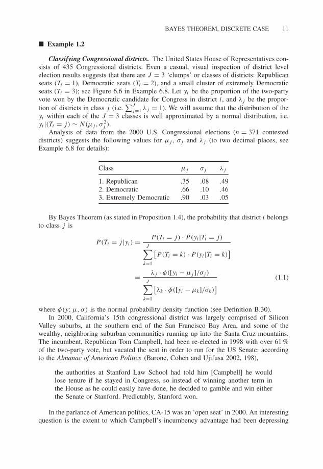
� Example 1.2
Classifying Congressional districts. The United States House of Representatives con-sists of 435 Congressional districts. Even a casual, visual inspection of district levelelection results suggests that there are J = 3 ‘clumps’ or classes of districts: Republicanseats (Ti = 1), Democratic seats (Ti = 2), and a small cluster of extremely Democraticseats (Ti = 3); see Figure 6.6 in Example 6.8. Let yi be the proportion of the two-partyvote won by the Democratic candidate for Congress in district i, and λj be the propor-tion of districts in class j (i.e.
∑Jj=1 λj = 1). We will assume that the distribution of the
yi within each of the J = 3 classes is well approximated by a normal distribution, i.e.yi |(Ti = j) ∼ N(μj , σ
2j ).
Analysis of data from the 2000 U.S. Congressional elections (n = 371 contesteddistricts) suggests the following values for μj , σj and λj (to two decimal places, seeExample 6.8 for details):
Class μj σj λj
1. Republican .35 .08 .492. Democratic .66 .10 .463. Extremely Democratic .90 .03 .05
By Bayes Theorem (as stated in Proposition 1.4), the probability that district i belongsto class j is
P(Ti = j |yi) = P(Ti = j) · P(yi |Ti = j)
J∑k=1
[P(Ti = k) · P(yi |Ti = k)
]
= λj · φ([yi − μj ]/σj )
J∑k=1
[λk · φ([yi − μk]/σk)
] (1.1)
where φ(y; μ, σ) is the normal probability density function (see Definition B.30).In 2000, California’s 15th congressional district was largely comprised of Silicon
Valley suburbs, at the southern end of the San Francisco Bay Area, and some of thewealthy, neighboring suburban communities running up into the Santa Cruz mountains.The incumbent, Republican Tom Campbell, had been re-elected in 1998 with over 61 %of the two-party vote, but vacated the seat in order to run for the US Senate: accordingto the Almanac of American Politics (Barone, Cohen and Ujifusa 2002, 198),
the authorities at Stanford Law School had told him [Campbell] he wouldlose tenure if he stayed in Congress, so instead of winning another term inthe House as he could easily have done, he decided to gamble and win eitherthe Senate or Stanford. Predictably, Stanford won.
In the parlance of American politics, CA-15 was an ‘open seat’ in 2000. An interestingquestion is the extent to which Campbell’s incumbency advantage had been depressing
12 THE FOUNDATIONS OF BAYESIAN INFERENCE
Democratic vote share. With no incumbent contesting the seat in 2000, it is arguable thatthe 2000 election would provide a better gauge of the district’s type. The Democraticcandidate, Mike Honda, won with 56 % of the two-party vote. So, given that yi = .56,to which class of congressional district should we assign CA-15? An answer is given bysubstituting the estimates given in the above table into the version of Bayes Theoremgiven in Equation 1.1: to two decimal places we have
P(Ti = 1|yi = .56) =.49 × φ([.56 − .35]/.07)
.49 × φ([.56 − .35]/.08) + .46 × φ([.56 − .66]/.10) + .05 × φ([.56 − .90]/.03)
= .49 × .11
(.49 × .11) + (.46 × 2.46) + (.05 × 9.7 × 10−27)
= .05
1.18= .04
P(Ti = 2|yi = .56) = .46 × 2.46
1.18= .96
P(Ti = 3|yi = .56) = .05 × 9.7 × 10−27
1.18≈ 0
0.2 0.4 0.6 0.8
0.0
0.2
0.4
0.6
0.8
1.0
Democratic Vote Share
Pos
terio
r P
roba
bilit
y of
Cla
ss M
embe
rshi
p
Republican Democratic
Extremely Democratic
CA-15
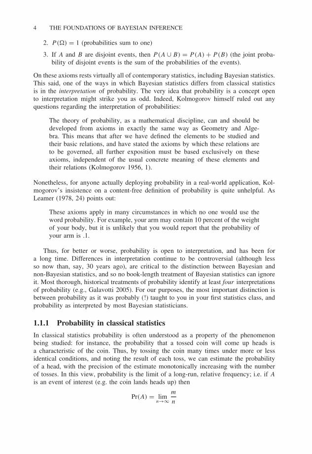
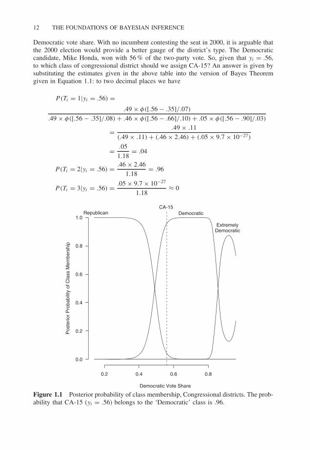
Figure 1.1 Posterior probability of class membership, Congressional districts. The prob-ability that CA-15 (yi = .56) belongs to the ‘Democratic’ class is .96.
BAYES THEOREM, CONTINUOUS PARAMETER 13
That is, the posterior probability that CA-15 belongs to the ‘Democratic’ class is .96. Notethat the result in CA-15, yi = .56 lies a long way from the ‘extremely Democratic’ class(μ3 = .90, σ3 = .03) and so the probability of assigning CA-15 to that class is virtuallyzero.
This calculation can be repeated for any plausible value of yi , and hence over anyrange of plausible values for yi , showing how posterior classification probabilities changeas a function of yi . Figure 1.1 presents a graph of the posterior probability of membershipin each of three classes of congressional district, as Democratic congressional vote shareranges over the values observed in the 2000 election. We will return to this example inChapter 5.
1.4 Bayes theorem, continuous parameter
In most analyses in the social sciences, we want to learn about a continuous parameter,rather than the discrete parameters considered in the discussion thus far. Examples includethe mean of a continuous variable, a proportion (a continuous parameter on the unitinterval), a correlation, or a regression coefficient. In general, let the unknown parameterbe θ and denote the data available for analysis as y = (y1, . . . , yn)
′. In the case ofcontinuous parameters, beliefs about the parameter are represented as probability densityfunctions or pdfs (see Definition B.12); we denote the prior pdf as p(θ) and the posteriorpdf as p(θ |y).
Then, Bayes Theorem for a continuous parameter is as follows:
Proposition 1.5 (Bayes Theorem, continuous parameter).
p(θ |y) = p(y|θ)p(θ)∫p(y|θ)p(θ)dθ
Proof. By the multiplication rule of probability (Proposition 1.1),
p(θ, y) = p(θ |y)p(y) = p(y|θ)p(θ), (1.2)
where all these densities are assumed to exist and have the properties p(z) > 0 and∫p(z)dz = 1 (i.e. are proper probability densities, see Definitions B.12 and B.13). The
result follows by re-arranging the quantities in Equation 1.2 and noting that p(y) =∫p(y, θ)dθ = ∫
p(y|θ)p(θ)dθ . �
Bayes Theorem for continuous parameters is more commonly expressed as follows,perhaps the most important formula in this book:
p(θ |y) ∝ p(y|θ)p(θ), (1.3)
where the constant of proportionality is[∫p(y|θ)p(θ)dθ
]−1
14 THE FOUNDATIONS OF BAYESIAN INFERENCE
i.e. ensuring that the posterior density integrates to one, as a proper probability densitymust (again, see Definitions B.12 and B.13).
The first term on the right hand side of Equation 1.3 is the likelihood function (seeDefinition B.16), the probability density of the data y, considered as a function of θ . Thus,we can state this version of Bayes Theorem in words, providing the ‘Bayesian mantra’,
the posterior is proportional to the prior times the likelihood .
This formulation of Bayes Rule highlights a particularly elegant feature of the Bayesianapproach, showing how the likelihood function p(y|θ) can be ‘inverted’ to generate aprobability statement about θ , given data y.
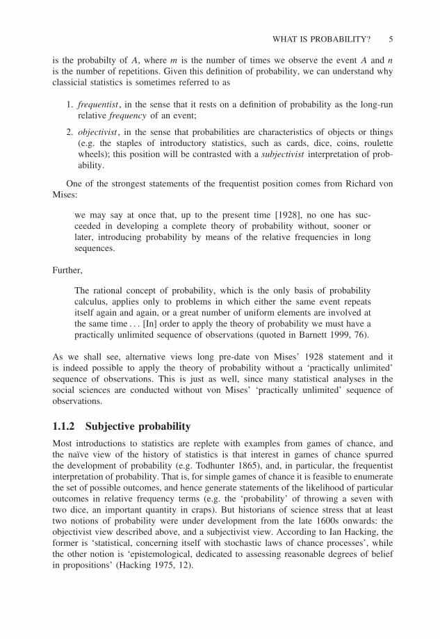
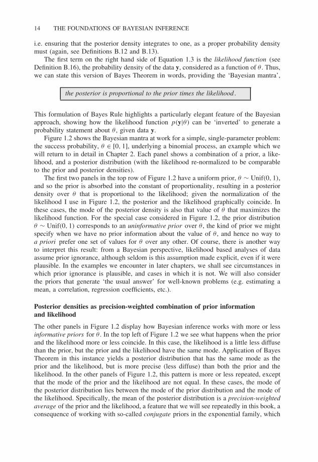
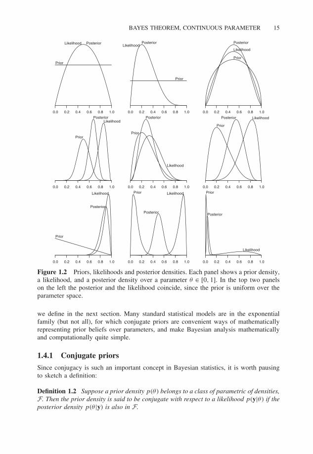
Figure 1.2 shows the Bayesian mantra at work for a simple, single-parameter problem:the success probability, θ ∈ [0, 1], underlying a binomial process, an example which wewill return to in detail in Chapter 2. Each panel shows a combination of a prior, a like-lihood, and a posterior distribution (with the likelihood re-normalized to be comparableto the prior and posterior densities).
The first two panels in the top row of Figure 1.2 have a uniform prior, θ ∼ Unif(0, 1),and so the prior is absorbed into the constant of proportionality, resulting in a posteriordensity over θ that is proportional to the likelihood; given the normalization of thelikelihood I use in Figure 1.2, the posterior and the likelihood graphically coincide. Inthese cases, the mode of the posterior density is also that value of θ that maximizes thelikelihood function. For the special case considered in Figure 1.2, the prior distributionθ ∼ Unif(0, 1) corresponds to an uninformative prior over θ , the kind of prior we mightspecify when we have no prior information about the value of θ , and hence no way toa priori prefer one set of values for θ over any other. Of course, there is another wayto interpret this result: from a Bayesian perspective, likelihood based analyses of dataassume prior ignorance, although seldom is this assumption made explicit, even if it wereplausible. In the examples we encounter in later chapters, we shall see circumstances inwhich prior ignorance is plausible, and cases in which it is not. We will also considerthe priors that generate ‘the usual answer’ for well-known problems (e.g. estimating amean, a correlation, regression coefficients, etc.).
Posterior densities as precision-weighted combination of prior informationand likelihood
The other panels in Figure 1.2 display how Bayesian inference works with more or lessinformative priors for θ . In the top left of Figure 1.2 we see what happens when the priorand the likelihood more or less coincide. In this case, the likelihood is a little less diffusethan the prior, but the prior and the likelihood have the same mode. Application of BayesTheorem in this instance yields a posterior distribution that has the same mode as theprior and the likelihood, but is more precise (less diffuse) than both the prior and thelikelihood. In the other panels of Figure 1.2, this pattern is more or less repeated, exceptthat the mode of the prior and the likelihood are not equal. In these cases, the mode ofthe posterior distribution lies between the mode of the prior distribution and the mode ofthe likelihood. Specifically, the mean of the posterior distribution is a precision-weightedaverage of the prior and the likelihood, a feature that we will see repeatedly in this book, aconsequence of working with so-called conjugate priors in the exponential family, which
BAYES THEOREM, CONTINUOUS PARAMETER 15
Prior
Likelihood Posterior
0.0 0.2 0.4 0.6 0.8 1.0
Prior
LikelihoodPosterior
0.0 0.2 0.4 0.6 0.8 1.0
Prior
Likelihood
Posterior
0.0 0.2 0.4 0.6 0.8 1.0
Prior
LikelihoodPosterior
0.0 0.2 0.4 0.6 0.8 1.0
Prior
Likelihood
Posterior
0.0 0.2 0.4 0.6 0.8 1.0
Prior
LikelihoodPosterior
0.0 0.2 0.4 0.6 0.8 1.0
Prior
Likelihood
Posterior
0.0 0.2 0.4 0.6 0.8 1.0
Prior Likelihood
Posterior
0.0 0.2 0.4 0.6 0.8 1.0
Prior
Likelihood
Posterior
0.0 0.2 0.4 0.6 0.8 1.0
Figure 1.2 Priors, likelihoods and posterior densities. Each panel shows a prior density,a likelihood, and a posterior density over a parameter θ ∈ [0, 1]. In the top two panelson the left the posterior and the likelihood coincide, since the prior is uniform over theparameter space.
we define in the next section. Many standard statistical models are in the exponentialfamily (but not all), for which conjugate priors are convenient ways of mathematicallyrepresenting prior beliefs over parameters, and make Bayesian analysis mathematicallyand computationally quite simple.
1.4.1 Conjugate priors
Since conjugacy is such an important concept in Bayesian statistics, it is worth pausingto sketch a definition:
Definition 1.2 Suppose a prior density p(θ) belongs to a class of parametric of densities,F. Then the prior density is said to be conjugate with respect to a likelihood p(y|θ) if theposterior density p(θ |y) is also in F.
16 THE FOUNDATIONS OF BAYESIAN INFERENCE
Of course, this definition rests on the unstated definition of a ‘class of parametricdensities’, and so is not as complete as one would prefer, but a thorough explanationinvolves more technical detail than is warranted for now. Examples are perhaps the bestway to illustrate the simplicity that conjugacy brings to a Bayesian analysis. And to thisend, all the examples in Chapter 2 use priors that are conjugate with respect to theirrespective likelihoods.
In particular, the examples in Figure 1.2 show the results of a Bayesian analysis ofbinomial data (n independent realizations of a binary process, also known as Bernoullitrials, such as coin flipping), for which the unknown parameter is θ ∈ [0, 1], the proba-bility of a ‘success’ on any given trial. For the likelihood function formed with binomialdata, any Beta density (see Definition B.28) over θ is a conjugate prior: that is, if priorbeliefs about θ can be represented as a Beta density, then after those beliefs have beenupdated (via Bayes Rule) in light of the binomial data, posterior beliefs about θ are alsocharacterized by a Beta density. In Section 2.1 we consider the Bayesian analysis ofbinomial data in considerable detail.
For now, one of the important features of conjugacy is the one that appears graphi-cally in Figure 1.2: for a wide class of problems (i.e. when conjugacy holds), Bayesianstatistical inference is equivalent to combining information, marrying the information inthe prior with the information in the data, with the relative contributions of prior and datato the posterior being proportional to their respective precisions. That is, Bayesian analy-sis with conjugate priors over a parameter θ is equivalent to taking a precision-weightedaverage of prior information about θ and the information in the data about θ .
Thus, when prior beliefs about θ are ‘vague’, ‘diffuse’, or, in the limit, uninformative,the posterior density will be dominated by the likelihood (i.e. the data contains much moreinformation than the prior about the parameters); e.g. the lower left panel of Figure 1.2.In the limiting case of an uninformative prior, the only information about the parameteris that in the data, and the posterior has the same shape as the likelihood function. Whenprior information is available, the posterior incorporates it, and rationally, in the senseof being consistent with the laws of probability via Bayes Theorem. In fact, when priorbeliefs are quite precise relative to the data, it is possible that the likelihood is largelyignored, and the posterior distribution will look almost exactly like the prior, as it shouldin such a case; e.g. see the lower right panel of Figure 1.2. In the limiting case of adegenerate, infinitely-precise, ‘spike prior’ (all prior probability concentrated on a point),the data are completely ignored, and the posterior is also a degenerate ‘spike’ distribution.Should you hold such a dogmatic prior, no amount of data will ever result in you changingyour mind about the issue.
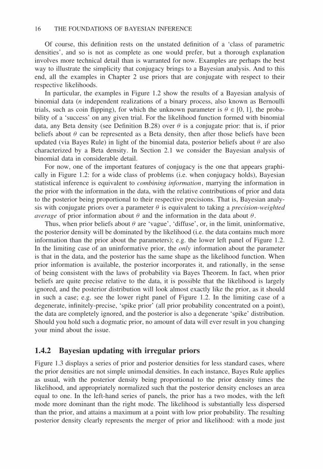
1.4.2 Bayesian updating with irregular priors
Figure 1.3 displays a series of prior and posterior densities for less standard cases, wherethe prior densities are not simple unimodal densities. In each instance, Bayes Rule appliesas usual, with the posterior density being proportional to the prior density times thelikelihood, and appropriately normalized such that the posterior density encloses an areaequal to one. In the left-hand series of panels, the prior has a two modes, with the leftmode more dominant than the right mode. The likelihood is substantially less dispersedthan the prior, and attains a maximum at a point with low prior probability. The resultingposterior density clearly represents the merger of prior and likelihood: with a mode just
BAYES THEOREM, CONTINUOUS PARAMETER 17
Prior
Likelihood
Posterior
Prior
Likelihood
Posterior
Prior
Likelihood
Posterior
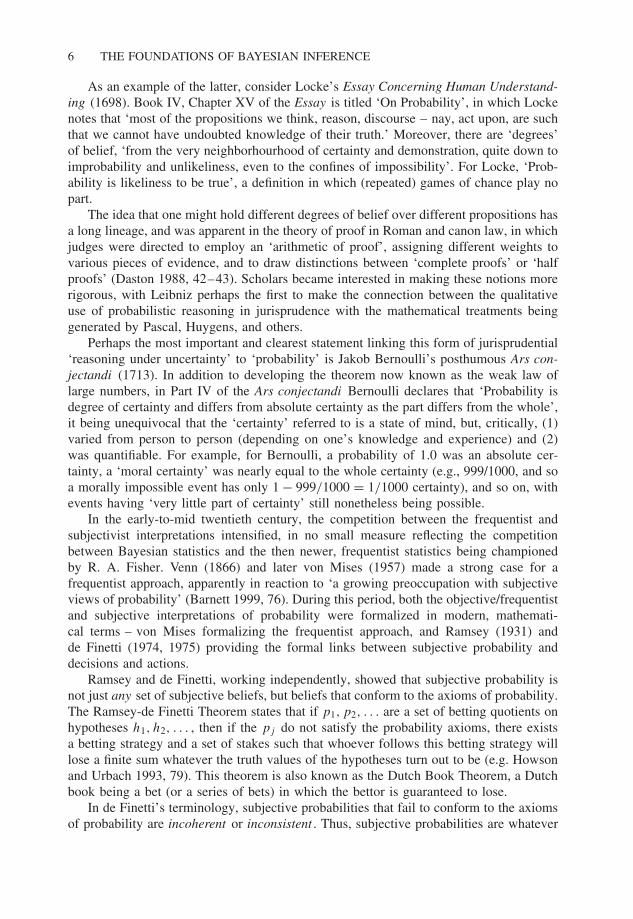
Figure 1.3 Priors, likelihoods and posterior densities for non-standard cases. Eachcolumn of panels shows the way Bayes Rule combines prior information (top) with infor-mation in the data (characterized by the likelihood, center) to yield a posterior density(lower panels).
to the left of the mode of the likelihood function, and a smaller mode just to the right ofthe mode of the likelihood function. The middle column of panels in Figure 1.3 shows asymmetric case: the prior is bimodal but symmetric around a trough corresponding to themode of the likelihood function, resulting in a bimodal posterior distribution, but withmodes shrunk towards the mode of the likelihood. In this case, the information in thedata about θ combines with the prior information to reduce the depth of the trough in theprior density, and to give substantially less weight to the outlying values of θ that receivehigh prior probability. In the right-hand column of Figure 1.3 an extremely flamboyantprior distribution (but one that is nonetheless symmetric about its mean) combines withthe skewed likelihood to produce the trimodal posterior density, with the posterior modeslocated in regions with relatively high likelihood. Although this prior (and posterior) are
18 THE FOUNDATIONS OF BAYESIAN INFERENCE
somewhat fanciful (in the sense that it is hard to imagine those densities correspondingto beliefs over a parameter), the central idea remains the same: Bayes Rule governs themapping from prior to posterior through the data. Implementing Bayes Rule may bedifficult when the prior is not conjugate to the likelihood, but, as we shall see, this iswhere modern computational tools are particularly helpful (see Chapter 3).
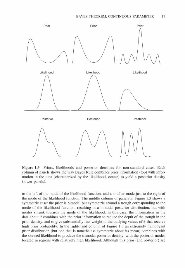
1.4.3 Cromwell’s Rule
Note also that via Bayes Rule, if a particular region of the parameter space has zero priorprobability, then it also has zero posterior probability. This feature of Bayesian updatinghas been dubbed ‘Cromwell’s Rule’ by Lindley (1985). After the English deposed, triedand executed Charles I in 1649, the Scots invited Charles’ son, Charles II, to become king.The English regarded this as a hostile act, and Oliver Cromwell led an army north. Priorto the outbreak of hostilities, Cromwell wrote to the synod of the Church of Scotland,‘I beseech you, in the bowels of Christ, consider it possible that you are mistaken’. Therelevance of Cromwell’s plea to the Scots for our purposes comes from noting that a priorthat assigns zero probability to a hypothesis can never be revised; likewise, a hypothesiswith prior weight of 1.0 can never be refuted.
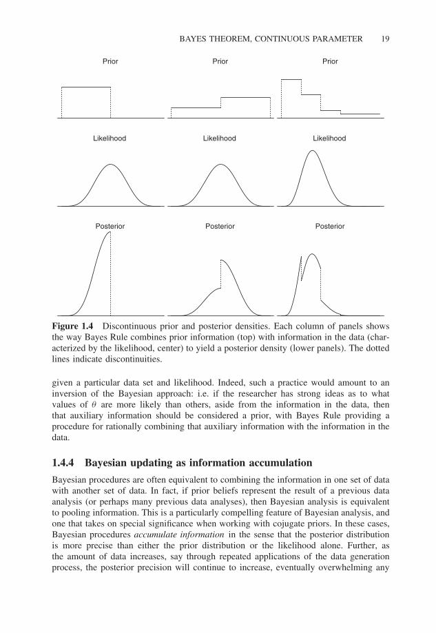
The operation of Cromwell’s Rule is particularly clear in the left-hand column ofpanels in Figure 1.4: the prior for θ is a uniform distribution over the left half of thesupport of the likelihood, and zero everywhere else. The resulting posterior assigns zeroprobability to values of θ assigned zero prior probability, and since the prior is uniformelsewhere, the posterior is a re-scaled version of the likelihood in this region of non-zeroprior probability, where the re-scaling follows from the constraint that the area underthe posterior distribution is one. The middle column of panels in Figure 1.4 shows aprior that has positive probability over all values of θ that has non-zero likelihood, anda discontinuity in the middle of the parameter space, with the left-half of the parameterspace supporting having half as much probability mass as the right-half. The resultingposterior has a discontinuity at the point where the prior does, but since the prior isotherwise uniform, the posterior inherits the shape of the likelihood on either side ofthe discontinuity, subject to the constraint (implied by the prior) that the posterior hastwice as much probability mass to the right of the discontinuity than to the left, andintegrates to one. The right-hand column of Figure 1.4 shows a more elaborate prior, astep function over the parameter space, decreasing to the right. The resulting posteriorhas discontinuities at the discontinuities in the prior, and some that are quite abrupt,depending on the conflict between the prior and likelihood in any particular segment ofthe prior.
The point here is that posterior distributions can sometimes look quite unusual,depending on the form of the prior and the likelihood for a particular problem. Thefact that a posterior distribution may have a peculiar shape is of no great concern ina Bayesian analysis: provided one is updating prior beliefs via Bayes Rule, all is well.Unusual looking posterior distributions might suggest that one’s prior distribution waspoorly specified, but, as a general rule, one should be extremely wary of engaging thiskind of procedure. Bayes Rule is a procedure for generating posterior distributions overparameters in light of data. Although one can always re-run a Bayesian analysis withdifferent priors (and indeed, this is usually a good idea), Bayesian procedures should notbe used to hunt for priors that generate the most pleasing looking posterior distribution,
BAYES THEOREM, CONTINUOUS PARAMETER 19
Prior
Likelihood
Posterior
Prior
Likelihood
Posterior
Prior
Likelihood
Posterior
Figure 1.4 Discontinuous prior and posterior densities. Each column of panels showsthe way Bayes Rule combines prior information (top) with information in the data (char-acterized by the likelihood, center) to yield a posterior density (lower panels). The dottedlines indicate discontinuities.
given a particular data set and likelihood. Indeed, such a practice would amount to aninversion of the Bayesian approach: i.e. if the researcher has strong ideas as to whatvalues of θ are more likely than others, aside from the information in the data, thenthat auxiliary information should be considered a prior, with Bayes Rule providing aprocedure for rationally combining that auxiliary information with the information in thedata.
1.4.4 Bayesian updating as information accumulation
Bayesian procedures are often equivalent to combining the information in one set of datawith another set of data. In fact, if prior beliefs represent the result of a previous dataanalysis (or perhaps many previous data analyses), then Bayesian analysis is equivalentto pooling information. This is a particularly compelling feature of Bayesian analysis, andone that takes on special significance when working with cojugate priors. In these cases,Bayesian procedures accumulate information in the sense that the posterior distributionis more precise than either the prior distribution or the likelihood alone. Further, asthe amount of data increases, say through repeated applications of the data generationprocess, the posterior precision will continue to increase, eventually overwhelming any
20 THE FOUNDATIONS OF BAYESIAN INFERENCE
non-degenerate prior; the upshot is that analysts with different (non-degenerate) priorbeliefs over a parameter will eventually find their beliefs coinciding, provided they (1)see enough data and (2) update their beliefs using Bayes Theorem (Blackwell and Dubins1962). In this way Bayesian analysis has been proclaimed as a model for scientific practice(e.g. Howson and Urbach 1993; Press 2003) acknowledging that while reasonable peoplemay differ (at least prior to seeing data), our views will tend to converge as scientificknowledge accumulates, provided we update our views rationally, consistent with thelaws of probability (i.e. via Bayes Theorem).
� Example 1.3
Drug testing, Example 1.1, continued. Suppose that the randomly selected subjectis someone you know personally, and you strongly suspect that she does not use the pro-hibited substance. Your prior over the hypothesis that she uses the prohibited substance isP(HU) = 1/1000. I have no special knowledge regarding the athlete, and use the baselineprior P(HU) = .03. After the positive test result, my posterior belief is P(HU |E) = .23,while yours is
P(HU |E) = P(HU)P (E|HU)∑i∈{U,∼U } P(Hi)P (E|Hi)
= .001 × .95
(.001 × .95) + (.999 × .10)
= .00095
.000095 + .0999≈ .009
A second test is performed. Now, our posteriors from the first test become the priorswith respect to the second test. Again, the subject tests positive, which we denote as theevent E′. My beliefs are revised as follows:
P(HU |E′) = .23 × .95
(.23 × .95) + (.77 × .10)
= .2185
.2185 + .077= .74,
while your beliefs are updated to
P(HU |E′) = .009 × .95
(.009 × .95) + (.991 × .10)
= .00855
.00855 + .0991≈ .079.
At this point, I am reasonably confident that the subject is using the prohibited substance,while you still attach reasonably low probability to that hypothesis. After a 3rd positive
PARAMETERS AS RANDOM VARIABLES, BELIEFS AS DISTRIBUTIONS 21
test your beliefs update to .45, and mine to .96. After a 4th positive test your beliefsupdate to .88 and mine to .996, and after a 5th test, your beliefs update to .99 and mine to.9996. That is, given this stream of evidence, common knowledge as to the properties ofthe test, and the fact that we are both rationally updating our beliefs via Bayes Theorem,our beliefs are converging.
In this case, given the stream of postitive test results, our posterior probabilitiesregarding the truth of HU are asymptotically approaching 1.0, albeit mine more quicklythan yours, given the low a priori probability you attached to HU . Note that with myprior, I required just two consecutive positive test results to revise my beliefs to thepoint where I considered it more likely than not that the subject is using the prohibitedsubstance, whereas you, with a much more skeptical prior, required four consecutivepostive tests.
It should also be noted that the specific pattern of results obtained in this case dependon the properties of the test. Tests with higher sensitivity and specificity would see ourbeliefs be revised more dramatically given the sequence of positive test results. Indeed,this is the objective of the design of diagnostic tests of various sorts: given a priorP(HU), what levels of sensitivity and specificity are required such that after just one ortwo positive tests, P(HU |E) exceeds a critical threshold where an action is justified. SeeExercise 1.2.
1.5 Parameters as random variables, beliefsas distributions
One of the critical ways in which Bayesian statistical inference differs from frequen-tist inference is immediately apparent from Equation 1.3 and the examples shown inFigure 1.2: the result of a Bayesian analysis, the posterior density p(θ |y) is just that, aprobability density. Given a subjectivist interpretation of probabilty that most Bayesiansadopt, the ‘randomness’ summarized by the posterior density is a reflection of theresearcher’s uncertainty over θ , conditional on having observed data y.
Contrast the frequentist approach, in which θ is not random, but a fixed (but unknown)property of a population from which we randomly sample data y. Repeated applicationsof the sampling process, if undertaken, would yield different y, and different samplebased estimates of θ , denoted θ = θ (y), this notation reminding us that estimates ofparameters are functions of data. In the frequentist scheme, the θ (y) vary randomlyacross data sets (or would, if repeated sampling was undertaken), while the parameter θ
is a constant feature of the population from which data sets are drawn. The distributionof values of θ that would result from repeated application of the sampling process iscalled the sampling distribution , and is the basis of inference in the frequentist approach;the standard deviation of the sampling distribution of θ is the standard error of θ , whichplays a key role in frequentist inference.
The Bayesian approach does not rely on how θ might vary over repeated applicationsof random sampling. Instead, Bayesian procedures center on a simple question: “whatshould I believe about θ in light of the data available for analysis, y?” The quantity θ (y)
has no special, intrinsic status in the Bayesian approach: as we shall see with specificexamples in Chapter 2, a least squares or maximum likelihood estimate of θ is a feature
22 THE FOUNDATIONS OF BAYESIAN INFERENCE
of the data that is usually helpful in computing the posterior distribution for θ . And,under some special circumstances, a least squares or maximum likelihood estimate of θ ,θ (y), will correspond to a Bayes estimate of θ (see Section 1.6.1). But the critical pointto grasp is that in the Bayesian approach, the roles of θ and θ are reversed relative totheir roles in classical, frequentist inference: θ is random, in the sense that the researcheris uncertain about its value, while θ is fixed, a feature of the data at hand.
1.6 Communicating the results of a Bayesian analysis
In a Bayesian analysis, all relevant information about θ after having analyzed the datais represented by the posterior density, p(θ |y). An important and interesting decision forthe Bayesian researcher is how to communicate posterior beliefs about θ .
In a world where journal space was less scarce than it is, researchers could simply pro-vide pictures of posterior distributions: e.g. density plots or histograms, as in Figure 1.2.Graphs are an extremely efficient way of presenting information, and, in the specific caseof probability distributions, let the researcher and readers see the location, dispersion andshape of the distribution, immediately gauging what regions of the parameter space aremore plausible than others, if any. This visualization strategy works well when θ is ascalar, but quickly becomes more problematic when working with multiple parameters,and so the posterior density is a multivariate distribution: i.e. we have
p(θ|y) = p(θ1, . . . , θk|y) ∝ p(θ)p(y|θ) (1.4)
Direct visualization is no longer feasible once k > 2: density plots or histograms havetwo-dimensional counterparts (e.g. contour or image plots, used throughout this book, andperspective plots), but we simply run out of dimensions at this point. As the dimensionof the parameter vector increases, we can graphically present one or two dimensionalslices of the posterior density. For problems with lots of parameters, this means that wemay have lots of pictures to present, consuming more journal space than even the mostsympathetic editor may be able to provide.
Thus, for models with lots of parameters, graphical presentation of the posteriordensity may not be feasible, at least not for all parameters. In these cases, numericalsummaries of the posterior density (or the marginal posterior densities specific to par-ticular parameters) are more feasible. Moreover, for most standard models, and if theresearcher’s prior beliefs have been expressed with conjugate priors, the analytic formof the posterior is known (indeed, as we shall see, this is precisely the attraction of con-jugate priors!). This means that for these standard cases, almost any interesting featureof the posterior can be computed directly: e.g., the mean, the mode, the standard devia-tion, or particular quantiles. For non-standard models, and/or for models where the priorsare not congujate, modern computational power lets us deploy Monte Carlo methods tocompute these features of posterior densities; see Chapter 3. Finally, it should be notedthat with large sample sizes, provided the prior is not degenerate, the posterior densitiesare usually well approximated by normal densities, for which it is straightforward tocompute numerical summaries (see Section 1.7). In this section I review proposals forsummarizing posterior densities.
COMMUNICATING THE RESULTS OF A BAYESIAN ANALYSIS 23
1.6.1 Bayesian point estimation
If a Bayesian point estimate is required – reducing the information in the posterior distri-bution to a single number – this can be done, although some regard the attempt to reducea posterior distribution to a single number as misguided and ad hoc. For instance,
While it [is] easy to demonstrate examples for which there can be no satis-factory point estimate, yet the idea is very strong among people in generaland some statisticians in particular that there is a need for such a quantity.To the idea that people like to have a single number we answer that usuallythey shouldn’t get it. Most people know they live in a statistical world andcommon parlance is full of words implying uncertainty. As in the case ofweather forecasts, statements about uncertain quantities ought to be made interms which reflect that uncertainty as nearly as possible (Box and Tiao 1973,309–10).
This said, it is convenient to report a point estimate when communicating the results of aBayesian analysis, and, so long as information summarizing the dispersion of the posteriordistribution is also provided (see Section 1.6.2, below), a Bayesian point estimate is quitea useful quantity to report.
The choice of which point summary of the posterior distribution to report can berationalized by drawing on (Bayesian) decision theory. Although we are interested in thespecific problem of choosing a single-number summary of a posterior distribution, thequestion of how to make rational choices under conditions of uncertainty is quite general,and we begin with a definition of loss:
Definition 1.3 (Loss Function). Let � be a set of possible states of nature θ , and leta ∈ A be actions availble to the researcher. Then define l(θ, a) as the loss to the researcherfrom taking action a when the state of nature is θ .
Recall that in the Bayesian approach, the researcher’s beliefs about plausible valuesfor θ are represented with a probability density function (or a probability mass function,if θ take discrete values), and, in particular, after looking at data y, beliefs about θ arerepresented by the posterior density p(θ |y). Generically, let p(θ) be a probability densityover θ , which in turn induces a density over losses. Averaging the losses over beliefsabout θ yields the Bayesian expected loss (Berger 1985, 8):
Definition 1.4 (Bayesian expected loss). If p(θ) is the probability density for θ ∈ � atthe time of decision making, the Bayesian expected loss of an action a is
�(p(θ), a) = E[l(θ, a)] =∫
�
l(θ, a)p(θ)dθ.
A special case is where the density p in Definition 1.4 is a posterior density:
Definition 1.5 (Posterior expected loss). Given a posterior density for θ , p(θ |y), theposterior expected loss of an action a is �(p(θ |y), a) = ∫
�l(θ, a)p(θ |y)dθ .
24 THE FOUNDATIONS OF BAYESIAN INFERENCE
A Bayesian rule for choosing among actions A is to select a ∈ A so to minimizeposterior expected loss. In the specific context of point estimation, the decision problemis to choose a Bayes estimate, θ , and so actions a ∈ A now index feasible values forθ ∈ �. The problem now is that since there are plausibly many different loss functionsone might adopt, there are plausibly many Bayesian point estimates one might choose toreport. If the chosen loss function is convex, then the corresponding Bayes estimate isunique (DeGroot and Rao 1963), so the choice of what Bayes estimate to report usuallyamounts to what (convex) loss function to adopt. We briefly consider some well-studiedcases.
Definition 1.6 (Quadratic loss). If θ ∈ � is a parameter of interest, and θ is an estimateof θ , then l(θ, θ ) = (θ − θ )2 is the quadratic loss arising from the use of the estimate θ
instead of θ .
With quadratic loss, we obtain the following useful result:
Proposition 1.6 (Posterior mean as a Bayes estimate under quadratic loss). Underquadratic loss the Bayes estimate of θ is the mean of the posterior density, i.e.θ = E(θ |y) = ∫
�θp(θ |y)dθ .
Proof. Quadratic loss (Definition 1.6) implies that the posterior expected loss is
�(θ, θ) =∫
�
(θ − θ )2p(θ |y)dθ.
and we seek to minimize this expression with respect to θ . Expanding the quadraticyields
�(θ, θ) =∫
�
θ2p(θ |y)dθ + θ2∫
�
p(θ |y)dθ − 2θ
∫�
θp(θ |y)dθ
=∫
�
θ2p(θ |y)dθ + θ2 − 2θE(θ |y),
Differentiate with respect to θ , noting that the first term does not involve θ . Then set thederivative to zero and solve for θ to establish the result. �
This result also holds for the case of performing inference with respect to a param-eter vector θ = (θ1, . . . , θK)′. In this more general case, we define a multidimensionalquadratic loss function as follows:
Definition 1.7 (Multidimensional quadratic loss). If θ ∈ RK is a parameter, and θ is an
estimate of θ, then the (multidimensional) quadratic loss is l(θ, θ) = (θ − θ)′Q(θ − θ)
where Q is a positive definite matrix.
Proposition 1.7 (Multidimensional posterior mean as Bayes estimate). Under quadraticloss (Definition 1.7), the posterior mean E(θ|y) = ∫
�θp(θ|y)dθ is the Bayes estimate
of θ.
COMMUNICATING THE RESULTS OF A BAYESIAN ANALYSIS 25
Proof. The posterior expected loss is �(θ, θ) = ∫�
(θ − θ)′Q(θ − θ)p(θ|y)dθ. Differen-tiating with respect to θ yields 2Q
∫�
(θ − θ)p(θ|y)dθ. Setting the derivative to zeroand re-arranging yields
∫�
(θ − θ)p(θ|y)dθ = 0 or∫�
θp(θ|y)dθ = ∫�
θp(θ|y)dθ. Theleft-hand side of this expression is just the mean of the posterior density, E(θ|y), and soE(θ|y) = ∫
�θp(θ|y)dθ = θ
∫�
p(θ|y)dθ = θ. �
Remark. This result holds irrespective of the specific weighting matrix Q, provided Q ispositive definite.
The mean of the posterior distribution is a popular choice among researchers seekingto quickly communicate features of the posterior distribution that results from a Bayesiandata analysis; we now understand the conditions under which this is a rational pointsummary of one’s beliefs over θ . Specifically, Proposition 1.6 rationalizes the choice ofthe mean of the posterior density as a Bayes estimate.
Of course, other loss functions rationalize other point summaries. Consider linear loss,possibly asymmetric around θ :
Definition 1.8 (Linear loss). If θ ∈ � is a parameter, and θ is a point estimate of θ , thenthe linear loss function is
l(θ, θ ) ={
k0(θ − θ ) if θ < θ
k1(θ − θ) if θ ≤ θ
Loss in absolute value results when k0 = k1 = 1, a special case of a class of sym-metric, linear loss functions (i.e. k0 = k1). Asymmetric linear loss results when k0 �= k1.
Proposition 1.8 (Bayes estimates under linear loss). Under linear loss (definition 1.8),the Bayes estimate of θ is the k1/(k0 + k1) quantile of p(θ |y), the θ such that P(θ ≤ θ ) =k0/(k0 + k1).
Proof. Following Bernardo and Smith (1994, 256), we seek the θ that minimizes
�(θ, θ) =∫
�
l(θ, θ)p(θ |y)dθ = k0
∫{θ<θ}
(θ − θ )p(θ |y)dθ + k1
∫{θ≤θ}
(θ − θ)p(θ |y)dθ.
Differentiating this expression with respect to θ and setting the result to zero yields
k0
∫{θ<θ}
p(θ |y)dθ = k1
∫{θ≤θ}
p(θ |y)dθ
Adding k0
∫{θ≤θ}
p(θ |y)dθ to both sides yields k0 = (k0 + k1)
∫{θ≤θ}
p(θ |y)dθ and so
re-arranging yields∫
{θ<θ}p(θ |y)dθ = k0/(k0 + k1). �
Note that with symmetric linear loss, we obtain the median of the posterior densityas the Bayes estimate. Asymmetric loss functions imply using quantiles other than themedian.
26 THE FOUNDATIONS OF BAYESIAN INFERENCE
� Example 1.4
Graduate Admissions. A professor reviews applications to a Ph.D. program. Theprofessor assumes that each applicant i ∈ {1, . . . , n} possesses ability θi . After reviewingthe applicants’ files (i.e. encountering data, or y), the professors’s beliefs regarding eachθi can be represented as a distribution p(θi |y). The professor’s loss function is asymmet-ric, since the professor has determined that it is 2.5 times as costly to overestimate anapplicant’s ability than it is to underestimate ability: i.e.
�(θ, θ) ={
θ − θ if θ > θ
2.5(θ − θ) if θ ≤ θ
Ability is measured on an arbitrary scale, normalized to have mean zero and standard devi-ation one across the applicant pool. Suppose that for applicant i, p(θi |y) ≈ N(1.8, 0.42),while for applicant j , p(θj |y) ≈ N(2.0, 1.02); i.e. there is considerably greater posterioruncertainty as to the ability of applicant j . Given the professors’s loss function, the Bayesestimate of θi is the 1/(1 + 2.5) = .286 quantile of the N(1.8, 0.42) posterior density, or1.57; for applicant j , the Bayes estimate is the .286 quantile of a N(2.0, 1.02) density, or1.43. Thus, although E(θj |y) >E(θi |y), the greater uncertainty associated with applicantj , when coupled with the asymmetric loss function, results in the professor assigning ahigher Bayes estimate to applicant j than to applicant i (i.e. θi < θj ).
1.6.2 Credible regions
Bayes estimates are an attempt to summarize beliefs over θ with a single number, pro-viding a rational, best guess as to the value of θ . But Bayes estimates do not conveyinformation as to the researcher’s uncertainty over θ , and indeed, this is why manyBayesian statisticians find Bayes estimates fundamentally unsatisfactory. To communi-cate a summary of prior or posterior uncertainty over θ , it is necessary to somehowsummarize information about the location and shape of the prior or posterior distribu-tion, p(θ). In particular, what is the set or region of more plausible values for θ? Moreformally, what is the region C ⊆ � that supports proportion α of the probability underp(θ)? Such a region is called a credible region:
Definition 1.9 (Credible region). A region C ⊆ � such that∫
C
p(θ)dθ = 1 − α, 0 ≤α ≤ 1 is a 100(1 − α)% credible region for θ .
For single-parameter problems (i.e. � ⊆ R), if C is not a set of disjoint intervals, thenC is a credible interval.
If p(θ) is a (prior/posterior) density, then C is a (prior/posterior) credible region.
There is trivially only one 100 % credible region, the entire support of p(θ). Butnon-trivial credible regions may not be unique. For example, suppose θ ∼ N(0, 1): itis obvious that there is no unique 100(1 − α)% credible region for any α ∈ (0, 1): anyinterval spanning 100(1 − α) percentiles will be such an interval. A solution to thisproblem comes from restricting attention to credible regions that have certain desirableproperties, including minimum volume (or, for a one dimensional parameter problem,
COMMUNICATING THE RESULTS OF A BAYESIAN ANALYSIS 27
minimum length) in the set of credible regions induced by a given choice of α, for aspecific p(θ). This kind of optimal credible region is called a highest probability densityregion , sometimes referred to as a HPD region or a ‘HDR’. The following definition ofa HPD region is standard and appears in many places in the literature, e.g. Box and Tiao(1973, 123) or Bernardo and Smith (1994, 260):
Definition 1.10 (Highest probability density interval). A region C ⊆ � is a 100(1 − α)%highest probability density region for θ under p(θ) if
1. P(θ ∈ C) = 1 − α
2. P(θ1) ≥ P(θ2), ∀ θ1 ∈ C, θ2 �∈ C
A 100(1 − α)% HPD region for a symmetric, unimodal density is obviously uniqueand symmetric around the mode. In fact, if p(θ) is a univariate normal density, a HPDis the same as a interval around the mean:
� Example 1.5
Suppose p(θ) ≡ N(a, b2). Then a 100(1 − α)% HPD region is the interval
(a − |zα|b, a + |zα|b)
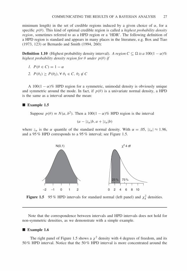
where zα is the α quantile of the standard normal density. With α = .05, |zα| ≈ 1.96,and a 95 % HPD corresponds to a 95 % interval; see Figure 1.5.
N(0,1) χ2 4 df
0 2 4 6 8 10
25% 75%
−2 −1 0 1 2
Figure 1.5 95 % HPD intervals for standard normal (left panel) and χ24 densities.
Note that the correspondence between intervals and HPD intervals does not hold fornon-symmetric densities, as we demonstrate with a simple example.
� Example 1.6
The right panel of Figure 1.5 shows a χ2 density with 4 degrees of freedom, and its50 % HPD interval. Notice that the 50 % HPD interval is more concentrated around the
28 THE FOUNDATIONS OF BAYESIAN INFERENCE
mode of the density, and has shorter length than the interval based on the 25th to 75thpercentiles of the density.
As the next two examples demonstrate, (1) the HPD need not be a connected set, buta collection of disjoint intervals (say, if p(θ) is not unimodal), and (2) the HPD need notbe unique.
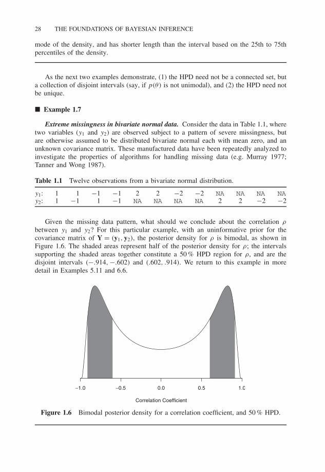
� Example 1.7
Extreme missingness in bivariate normal data. Consider the data in Table 1.1, wheretwo variables (y1 and y2) are observed subject to a pattern of severe missingness, butare otherwise assumed to be distributed bivariate normal each with mean zero, and anunknown covariance matrix. These manufactured data have been repeatedly analyzed toinvestigate the properties of algorithms for handling missing data (e.g. Murray 1977;Tanner and Wong 1987).
Table 1.1 Twelve observations from a bivariate normal distribution.
y1: 1 1 −1 −1 2 2 −2 −2 NA NA NA NAy2: 1 −1 1 −1 NA NA NA NA 2 2 −2 −2
Given the missing data pattern, what should we conclude about the correlation ρ
between y1 and y2? For this particular example, with an uninformative prior for thecovariance matrix of Y = (y1, y2), the posterior density for ρ is bimodal, as shown inFigure 1.6. The shaded areas represent half of the posterior density for ρ; the intervalssupporting the shaded areas together constitute a 50 % HPD region for ρ, and are thedisjoint intervals (−.914, −.602) and (.602, .914). We return to this example in moredetail in Examples 5.11 and 6.6.
Correlation Coefficient
−1.0 −0.5 0.0 0.5 1.0
Figure 1.6 Bimodal posterior density for a correlation coefficient, and 50 % HPD.
ASYMPTOTIC PROPERTIES OF POSTERIOR DISTRIBUTIONS 29
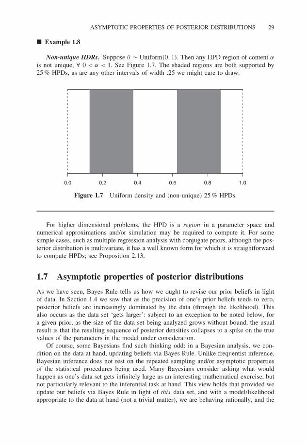
� Example 1.8
Non-unique HDRs. Suppose θ ∼ Uniform(0, 1). Then any HPD region of content α
is not unique, ∀ 0 < α < 1. See Figure 1.7. The shaded regions are both supported by25 % HPDs, as are any other intervals of width .25 we might care to draw.
0.0 0.2 0.4 0.6 0.8 1.0
Figure 1.7 Uniform density and (non-unique) 25 % HPDs.
For higher dimensional problems, the HPD is a region in a parameter space andnumerical approximations and/or simulation may be required to compute it. For somesimple cases, such as multiple regression analysis with conjugate priors, although the pos-terior distribution is multivariate, it has a well known form for which it is straightforwardto compute HPDs; see Proposition 2.13.
1.7 Asymptotic properties of posterior distributions
As we have seen, Bayes Rule tells us how we ought to revise our prior beliefs in lightof data. In Section 1.4 we saw that as the precision of one’s prior beliefs tends to zero,posterior beliefs are increasingly dominated by the data (through the likelihood). Thisalso occurs as the data set ‘gets larger’: subject to an exception to be noted below, fora given prior, as the size of the data set being analyzed grows without bound, the usualresult is that the resulting sequence of posterior densities collapses to a spike on the truevalues of the parameters in the model under consideration.
Of course, some Bayesians find such thinking odd: in a Bayesian analysis, we con-dition on the data at hand, updating beliefs via Bayes Rule. Unlike frequentist inference,Bayesian inference does not rest on the repeated sampling and/or asymptotic propertiesof the statistical procedures being used. Many Bayesians consider asking what wouldhappen as one’s data set gets infinitely large as an interesting mathematical exercise, butnot particularly relevant to the inferential task at hand. This view holds that provided weupdate our beliefs via Bayes Rule in light of this data set, and with a model/likelihoodappropriate to the data at hand (not a trivial matter), we are behaving rationally, and the
30 THE FOUNDATIONS OF BAYESIAN INFERENCE
repeated sampling or asymptotic properties of our inferences are second order concerns.Some Bayesians even go further, arguing that models and parameters have no objective,exterior reality, but are mathematical fictions we conjure so as to help us make probabil-ity assignments over data (we explore this ‘subjectivist’ position further in §1.9), and soquestions such as consistency are moot.
My own position – echoing that of Diaconis and Freedman (1986a, 11) – is that evensubjectivist Bayesians ought to consider asymptotic properties of Bayes estimates, sinceif Bayesian inference is to be a model of scientific practice, we should be able to establishthe convergence of (initially disparate) opinions as relevant evidence accumulates.
So what can we say about Bayesian inferences, asymptotically? The key idea hereis that subject to some regularity conditions, as the data set grows without bound, theposterior density is increasingly dominated by the contribution from the data throughthe likelihood function, and the standard asymptotic properties of maximum likelihoodestimators apply to the posterior density. These properties include
• consistency, at least in the sense that the posterior density is increasingly concen-trated around the true parameter value as n → ∞; or, in the additional sense ofBayes point estimators of θ (Section 1.6.1) being consistent;
• asymptotic normality, i.e. p(θ |y) tends to a normal distribution as n → ∞.
There is a large literature establishing the conditions under which frequentist andBayesian procedures coincide, at least asymptotically. These results are too technical to bereviewed in any detail in this text; see, for instance, Bernardo and Smith (1994, ch. 5) forstatements of necessary regularity conditions and proofs of the main results and referencesto the literature. Diaconis and Freedman (1986a,b) provide some counter-examples to theconsistency results; the ‘incidental parameters’ problem (Neyman and Scott 1948) isone such counter-example which we briefly return to in Section 9.1.2. I provide a briefillustration of ‘Bayesian consistency’ with two examples, below, and sketch a proof of a‘Bayesian central limit theorem’ in the Appendix.
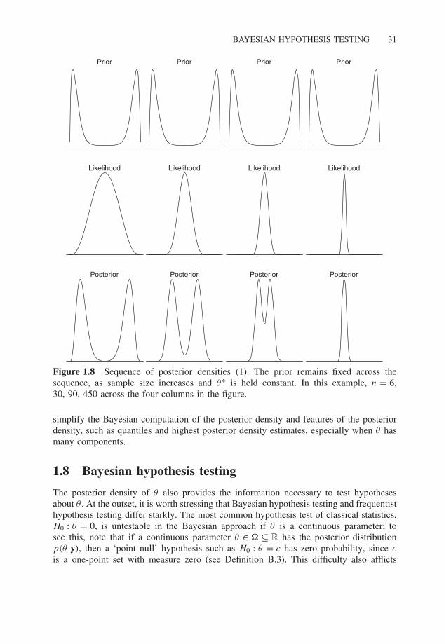
Bayesian consistency works as follows. Suppose the true value of θ is θ∗. Thenprovided the prior distribution p(θ) does not place zero probability mass on θ∗ (say, fora discrete parameter), or on a neigborhood of θ∗ (say, for a continuous parameter), thenas n → ∞, the posterior will be increasingly dominated by the contribution from thelikelihood, which, under suitable regularity conditions, tends to a spike on θ∗.
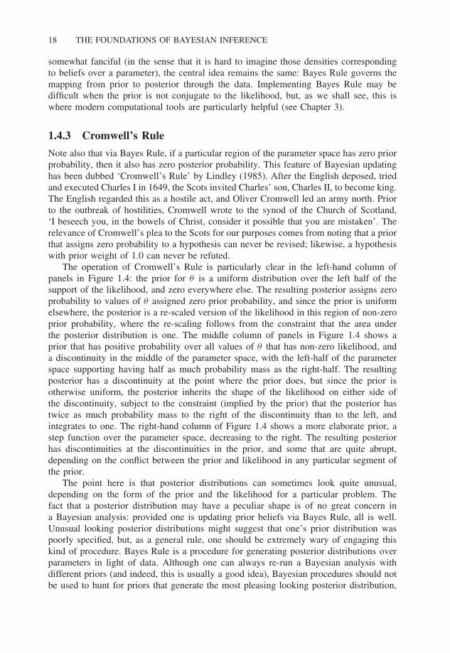
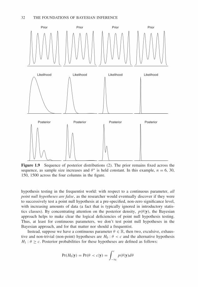
Figures 1.8 and 1.9 graphically demonstrate the Bayesian version of consistency asdescribed above. In each case, the prior is held constant as the sample size increases,leading to a progressively tighter correspondence between the posterior and the likelihood.Even with modest amounts of data, the multimodality of the priors are being overwhelmedby the information in the data, and the likelihood and posterior are collapsing to a spikeon θ∗.
Although the scale used in Figures 1.8 and 1.9 doesn’t make it clear, the likelihoodsand posterior in the Figures are also tending to normal distributions: re-scaling by theusual
√n would make this clear. The fact that posterior densities start to take on a
normal shape as n → ∞ is particularly helpful. The normal is an extremely well-studieddistribution, and completely characterized by its first two moments. This can drastically
BAYESIAN HYPOTHESIS TESTING 31
Prior
Likelihood
Posterior
Prior
Likelihood
Posterior
Prior
Likelihood
Posterior
Prior
Likelihood
Posterior
Figure 1.8 Sequence of posterior densities (1). The prior remains fixed across thesequence, as sample size increases and θ∗ is held constant. In this example, n = 6,30, 90, 450 across the four columns in the figure.
simplify the Bayesian computation of the posterior density and features of the posteriordensity, such as quantiles and highest posterior density estimates, especially when θ hasmany components.
1.8 Bayesian hypothesis testing
The posterior density of θ also provides the information necessary to test hypothesesabout θ . At the outset, it is worth stressing that Bayesian hypothesis testing and frequentisthypothesis testing differ starkly. The most common hypothesis test of classical statistics,H0 : θ = 0, is untestable in the Bayesian approach if θ is a continuous parameter; tosee this, note that if a continuous parameter θ ∈ � ⊆ R has the posterior distributionp(θ |y), then a ‘point null’ hypothesis such as H0 : θ = c has zero probability, since c
is a one-point set with measure zero (see Definition B.3). This difficulty also afflicts
32 THE FOUNDATIONS OF BAYESIAN INFERENCE
Prior
Likelihood
Posterior
Prior
Likelihood
Posterior
Prior
Likelihood
Posterior
Prior
Likelihood
Posterior
Figure 1.9 Sequence of posterior distributions (2). The prior remains fixed across thesequence, as sample size increases and θ∗ is held constant. In this example, n = 6, 30,150, 1500 across the four columns in the figure.
hypothesis testing in the frequentist world: with respect to a continuous parameter, allpoint null hypotheses are false, as the researcher would eventually discover if they wereto successively test a point null hypothesis at a pre-specified, non-zero significance level,with increasing amounts of data (a fact that is typically ignored in introductory statis-tics classes). By concentrating attention on the posterior density, p(θ |y), the Bayesianapproach helps to make clear the logical deficiencies of point null hypothesis testing.Thus, at least for continuous parameters, we don’t test point null hypotheses in theBayesian approach, and for that matter nor should a frequentist.
Instead, suppose we have a continuous parameter θ ∈ R, then two, exculsive, exhaus-tive and non-trivial (non-point) hypotheses are H0 : θ < c and the alternative hypothesisH1 : θ ≥ c. Posterior probabilities for these hypotheses are defined as follows:
Pr(H0|y) = Pr(θ < c|y) =∫ c
−∞p(θ |y)dθ
BAYESIAN HYPOTHESIS TESTING 33
and
Pr(H1|y) = Pr(θ ≥ c|y) =∫ ∞
c
p(θ |y)dθ.
For standard models, where conjugate priors have been deployed, these posterior proba-bilities are straightforward to compute; in other cases, modern computing power meansMonte Carlo methods can be deployed to assess these probabilities, as we will see inChapter 3.
The posterior probability of a hypothesis is something that only makes sense in aBayesian framework. There is no such corresponding quantity in a frequentist framework,although this is how a frequentist p-value is often misinterpreted. For a frequentist, θ
is a fixed but unknown number, and so hypotheses about θ are either true or false, andPr(H0|y) = 1 if H0 is true, and zero if it is not. As such, for a frequentist, the falsity ortruth of a hypothesis does not depend on the data, and so a quantity such as Pr(H0|y)
is meaningless. In contrast, for the Bayesian, θ is not fixed, but subject to (subjectiveprior/posterior) uncertainty, and so too is H0, and so the posterior probability Pr(H0|y) isquite useful. Indeed, one might argue that those types of posterior probability statementare exactly what one wants from a data analysis, letting us make statements of the sort‘how plausible is hypothesis H0 in light of these data?’ A frequentist p-value answersa different question: ‘how frequently would I observe a result at least as extreme as theone obtained if H0 were true?’, which is a statement about the plausibility of the datagiven the hypothesis. Turning this assessment into an assessment about the hypothesisrequires another step in the frequentist chain of reasoning (e.g. conclude H0 is false ifthe p-value falls below some preset level). Contrast the Bayesian procedure, which letsus assess the plausibility of H0 directly. A long line of papers contrasts p-values withBayesian posterior probabilities, arguing (as I have here) that many analysts interpret theformer as the latter, but that these two quantities can often be very different from oneanother; especially helpful papers on this score include Dickey (1977), Berger and Sellke(1987) and Berger (2003).
The following example provides a demonstration of Bayesian hypothesis testing usingdata from a survey. To help understand how Bayesian and frequentist approaches tohypothesis testing differ, a frequentist analysis is also provided.
� Example 1.9
Attitudes towards abortion. Agresti and Finlay (1997, 133) report that in the 1994General Social Survey, 1934 respondents were asked
Please tell me whether or not you think it should be possible for a pregnantwoman to obtain a legal abortion if the woman wants it for any reason.
Of the 1934 respondents, 895 reported ‘yes’ and 1039 said ‘no’. Let θ be the unknownpopulation proportion of respondents who agree with the proposition in the survey item,that a pregnant woman should be able to obtain an abortion if the woman wants it forany reason. The question of interest is whether a majority of the population supports theproposition in the survey item.
34 THE FOUNDATIONS OF BAYESIAN INFERENCE
Frequentist approach. The survey estimate of θ is θ = 895/1934 ≈ .46, the approxi-mation coming via rounding to two significant digits. Although the underlying data arebinomial (independent Bernoulli trials), with this large sample, the normal distributionprovides an excellent approximation to the frequentist sampling distribution of θ ; bino-mial data are considered in detail in Chapter 2. Suppose interest focuses on whether theunknown population proportion θ = .5. A typical frequentist approach to this questionis to test the null hypothesis H0 : θ = .5 against all other alternatives HA : θ �= .5, or aone-sided alternative HB : θ > .5. We would then ask how unlikely it is that one wouldsee the value of θ actually obtained, or an even more extreme value if H0 were true, bycentering the sampling distribution of θ at the hypothesized value. The standard deviationof the normal sampling distribution (the standard error of θ ) under H0 is
se(θH0) =√
θH0(1 − θH0)
n=
√.50 × (1 − .50)
1934≈ .011.
The realized value of θ is (.5 − .46)/.011 ≈ 3.64 standard errors away from the hypoth-esized value. Under a normal distribution, this an extremely rare event. Over repeatedapplications of random sampling, only a small proportion of estimates of θ will lie 3.64or more standard errors away from the hypothesized mean of the sampling distribution.This proportion is
2 ×∫ ∞
3.64φ(z)dz = 2 × [1 − �(3.64)] ≈ .00028,
where φ(·) and �(·) are the normal pdf and cdfs, respectively. Given this result, most (fre-quentist) analysts would reject the null hypothesis in favor of either alternative hypothesis,reporting the p-values for H0 against HA as .00028 and for H0 against HB as .00014.
Bayesian approach. The unknown parameter is θ ∈ [0, 1] and suppose we bring littleor no prior information to the analysis. In such a case, we know that the posteriordensity has the same shape as the likelihood, which with the large sample used here iswell approximated by a normal density (the details of Bayesian estimation and inferencefor a sample proportion are presented in Chapter 2), specifically, a normal distributioncentered on the maximum likelihood estimate of .46 with standard deviation .011; i.e.p(θ |y) ≈ N(.46, .0112) and inferences about θ are based on this distribution. We noteimmediately that most of the posterior probability mass lies below .5, suggesting that thehypothesis θ > .5 is not well-supported by the data. In fact, the posterior probability ofthis hypothesis is
Pr(θ > .5|y) =∫ ∞
.5p(θ |y)dθ =
∫ ∞
.5φ
(θ − .46
.011
)dθ = .00014.
That is, there is an apparent symmetry between the frequentist and Bayesian answers:in both instances, the ‘answer’ involved computing the same tail area probability of anormal distribution, with the probability of H0 under the Bayesian posterior distributioncorresponding with the p-value in the frequentist test of H0 against the one-sided alter-native HB ; see Figure 1.10. But this similarity really is only superficial. The Bayesianprobability is a statement about the researcher’s beliefs about θ , obtained via application
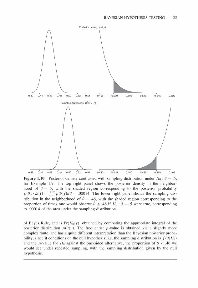
BAYESIAN HYPOTHESIS TESTING 35
0.42 0.44 0.46 0.48 0.50 0.52 0.54 0.495 0.500 0.505 0.510 0.515 0.520
0.42 0.44 0.46 0.48 0.50 0.52 0.54 0.440 0.445 0.450 0.455 0.460 0.465
Sampling distribution, f (q |q = .5)
Posterior density, p (q |y )
^
Figure 1.10 Posterior density contrasted with sampling distribution under H0 : θ = .5,for Example 1.9. The top right panel shows the posterior density in the neighbor-hood of θ = .5, with the shaded region corresponding to the posterior probabilityp(θ > .5|y) = ∫ ∞
.5 p(θ |y)dθ = .00014. The lower right panel shows the sampling dis-tribution in the neighborhood of θ = .46, with the shaded region corresponding to theproportion of times one would observe θ ≤ .46 if H0 : θ = .5 were true, correspondingto .00014 of the area under the sampling distribution.
of Bayes Rule, and is Pr(H0|y), obtained by computing the appropriate integral of theposterior distribution p(θ |y). The frequentist p-value is obtained via a slightly morecomplex route, and has a quite different interpretation than the Bayesian posterior proba-bility, since it conditions on the null hypothesis; i.e. the sampling distribution is f (θ |H0)
and the p-value for H0 against the one-sided alternative, the proportion of θ < .46 wewould see under repeated sampling, with the sampling distribution given by the nullhypothesis.
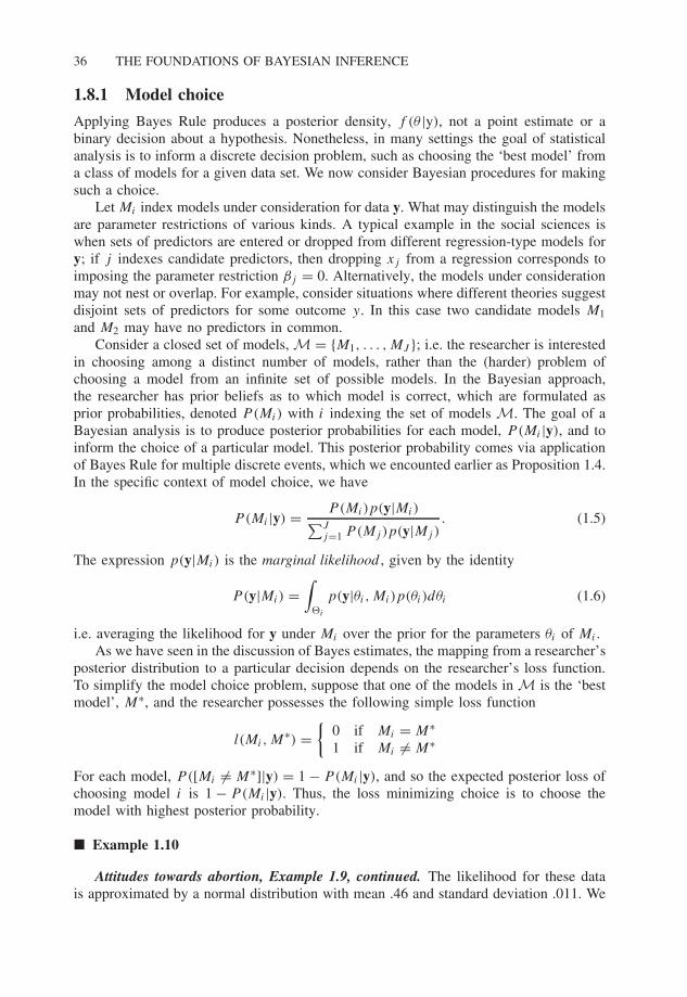
36 THE FOUNDATIONS OF BAYESIAN INFERENCE
1.8.1 Model choice
Applying Bayes Rule produces a posterior density, f (θ |y), not a point estimate or abinary decision about a hypothesis. Nonetheless, in many settings the goal of statisticalanalysis is to inform a discrete decision problem, such as choosing the ‘best model’ froma class of models for a given data set. We now consider Bayesian procedures for makingsuch a choice.
Let Mi index models under consideration for data y. What may distinguish the modelsare parameter restrictions of various kinds. A typical example in the social sciences iswhen sets of predictors are entered or dropped from different regression-type models fory; if j indexes candidate predictors, then dropping xj from a regression corresponds toimposing the parameter restriction βj = 0. Alternatively, the models under considerationmay not nest or overlap. For example, consider situations where different theories suggestdisjoint sets of predictors for some outcome y. In this case two candidate models M1
and M2 may have no predictors in common.Consider a closed set of models, M = {M1, . . . ,MJ }; i.e. the researcher is interested
in choosing among a distinct number of models, rather than the (harder) problem ofchoosing a model from an infinite set of possible models. In the Bayesian approach,the researcher has prior beliefs as to which model is correct, which are formulated asprior probabilities, denoted P(Mi) with i indexing the set of models M. The goal of aBayesian analysis is to produce posterior probabilities for each model, P(Mi |y), and toinform the choice of a particular model. This posterior probability comes via applicationof Bayes Rule for multiple discrete events, which we encounted earlier as Proposition 1.4.In the specific context of model choice, we have
P(Mi |y) = P(Mi)p(y|Mi)∑Jj=1 P(Mj)p(y|Mj)
. (1.5)
The expression p(y|Mi) is the marginal likelihood , given by the identity
P(y|Mi) =∫
�i
p(y|θi, Mi)p(θi)dθi (1.6)
i.e. averaging the likelihood for y under Mi over the prior for the parameters θi of Mi .As we have seen in the discussion of Bayes estimates, the mapping from a researcher’s
posterior distribution to a particular decision depends on the researcher’s loss function.To simplify the model choice problem, suppose that one of the models in M is the ‘bestmodel’, M∗, and the researcher possesses the following simple loss function
l(Mi, M∗) =
{0 if Mi = M∗1 if Mi �= M∗
For each model, P([Mi �= M∗]|y) = 1 − P(Mi |y), and so the expected posterior loss ofchoosing model i is 1 − P(Mi |y). Thus, the loss minimizing choice is to choose themodel with highest posterior probability.
� Example 1.10
Attitudes towards abortion, Example 1.9, continued. The likelihood for these datais approximated by a normal distribution with mean .46 and standard deviation .011. We
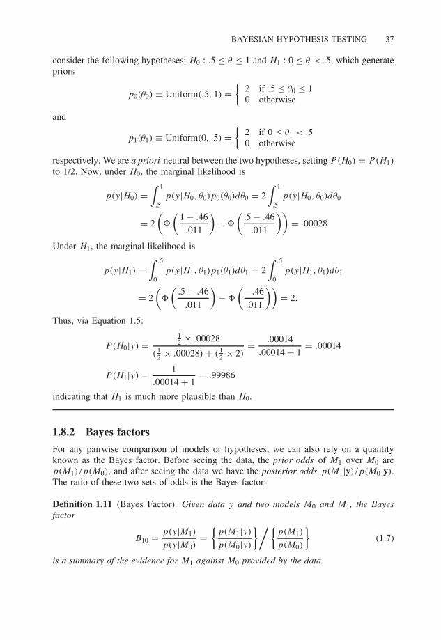
BAYESIAN HYPOTHESIS TESTING 37
consider the following hypotheses: H0 : .5 ≤ θ ≤ 1 and H1 : 0 ≤ θ < .5, which generatepriors
p0(θ0) ≡ Uniform(.5, 1) ={
2 if .5 ≤ θ0 ≤ 10 otherwise
and
p1(θ1) ≡ Uniform(0, .5) ={
2 if 0 ≤ θ1 < .50 otherwise
respectively. We are a priori neutral between the two hypotheses, setting P(H0) = P(H1)
to 1/2. Now, under H0, the marginal likelihood is
p(y|H0) =∫ 1
.5p(y|H0, θ0)p0(θ0)dθ0 = 2
∫ 1
.5p(y|H0, θ0)dθ0
= 2
(�
(1 − .46
.011
)− �
(.5 − .46
.011
))= .00028
Under H1, the marginal likelihood is
p(y|H1) =∫ .5
0p(y|H1, θ1)p1(θ1)dθ1 = 2
∫ .5
0p(y|H1, θ1)dθ1
= 2
(�
(.5 − .46
.011
)− �
(−.46
.011
))= 2.
Thus, via Equation 1.5:
P(H0|y) =12 × .00028
( 12 × .00028) + ( 1
2 × 2)= .00014
.00014 + 1= .00014
P(H1|y) = 1
.00014 + 1= .99986
indicating that H1 is much more plausible than H0.
1.8.2 Bayes factors
For any pairwise comparison of models or hypotheses, we can also rely on a quantityknown as the Bayes factor. Before seeing the data, the prior odds of M1 over M0 arep(M1)/p(M0), and after seeing the data we have the posterior odds p(M1|y)/p(M0|y).The ratio of these two sets of odds is the Bayes factor:
Definition 1.11 (Bayes Factor). Given data y and two models M0 and M1, the Bayesfactor
B10 = p(y|M1)
p(y|M0)=
{p(M1|y)
p(M0|y)
}/{p(M1)
p(M0)
}(1.7)
is a summary of the evidence for M1 against M0 provided by the data.
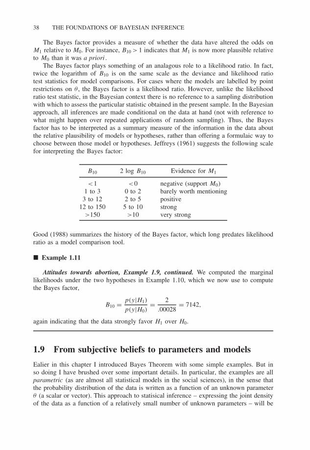
38 THE FOUNDATIONS OF BAYESIAN INFERENCE
The Bayes factor provides a measure of whether the data have altered the odds onM1 relative to M0. For instance, B10 > 1 indicates that M1 is now more plausible relativeto M0 than it was a priori .
The Bayes factor plays something of an analagous role to a likelihood ratio. In fact,twice the logarithm of B10 is on the same scale as the deviance and likelihood ratiotest statistics for model comparisons. For cases where the models are labelled by pointrestrictions on θ , the Bayes factor is a likelihood ratio. However, unlike the likelihoodratio test statistic, in the Bayesian context there is no reference to a sampling distributionwith which to assess the particular statistic obtained in the present sample. In the Bayesianapproach, all inferences are made conditional on the data at hand (not with reference towhat might happen over repeated applications of random sampling). Thus, the Bayesfactor has to be interpreted as a summary measure of the information in the data aboutthe relative plausibility of models or hypotheses, rather than offering a formulaic way tochoose between those model or hypotheses. Jeffreys (1961) suggests the following scalefor interpreting the Bayes factor:
B10 2 log B10 Evidence for M1
<1 <0 negative (support M0)1 to 3 0 to 2 barely worth mentioning
3 to 12 2 to 5 positive12 to 150 5 to 10 strong
>150 >10 very strong
Good (1988) summarizes the history of the Bayes factor, which long predates likelihoodratio as a model comparison tool.
� Example 1.11
Attitudes towards abortion, Example 1.9, continued. We computed the marginallikelihoods under the two hypotheses in Example 1.10, which we now use to computethe Bayes factor,
B10 = p(y|H1)
p(y|H0)= 2
.00028= 7142,
again indicating that the data strongly favor H1 over H0.
1.9 From subjective beliefs to parameters and models
Ealier in this chapter I introduced Bayes Theorem with some simple examples. But inso doing I have brushed over some important details. In particular, the examples are allparametric (as are almost all statistical models in the social sciences), in the sense thatthe probability distribution of the data is written as a function of an unknown parameterθ (a scalar or vector). This approach to statisical inference – expressing the joint densityof the data as a function of a relatively small number of unknown parameters – will be
FROM SUBJECTIVE BELIEFS TO PARAMETERS AND MODELS 39
familiar to many readers, and may not warrant justification or elaboration. But given thesubjectivist approach adopted here the question of how and why parameters and modelsenter the picture is not idle.
Recall that in the subjectivist approach championed by de Finetti (and adopted here),the idea that probability is a property of a coin, a die, or any other object under study,is regarded as metaphysical nonsense. All that is real is the data at hand. We may alsopossess knowledge (or at least beliefs) about how the data were generated. For instance,are the data real at all, or are they output of a computer simulation? Were the dataproduced via an experiment with random assignment to treatment and control groups, byrandom sampling from a specific population, or are the data a complete enumeration of apopulation? But everything else is a more or less convenient fiction created in the mindof the researcher including parameters and models .
To help grasp the issue a little more clearly, consider the following example. Acoin is flipped n times. The possible set of outcomes is S = {{H, T }1 × . . . × {H,T }n},with cardinality 2n. Assigning probabilities over the elements of S is a difficult task,if only because for any moderate to large value of n, 2n is a large number. Almostinstinctively, we start falling back on familar ways to simplify the problem. For example,reaching back to our introductory statistics classes, we would probably inquire ‘are thecoin flips independent?’ If satisfied that the coin flips are independent, we would thenfit a binomial model to the data, modeling the r flips coming up heads as a function ofa ‘heads’ probability θ , given the n flips. In a Bayesian analysis we would also have aprior density p(θ) as part of the model, and we would report the posterior density overp(θ |r, n) as the result of the analysis.
I now show that this procedure – using parameteric models to simplify dataanalysis – can be justified by recourse to a deeper principle called exchangeability . Inparticular, if data are ‘infinitely exchangeable’, then a Bayesian approach to modelingthe data is not only possible or desirable, but is actually implied by exchangeability.That is, prior distributions over parameters are not merely a ‘Bayesian addition’ to anotherwise classical analysis, but necessarily arise when one believes that the data areexchangeable. This is the key insight of one of the most important theorems in Bayesianstatistics – de Finetti’s Representation Theorem – which we will also encounter below.
1.9.1 Exchangeability
We begin with a definition:
Definition 1.12 (Finite exchangeability). The random quantities y1, . . . , yn are finitelyexchangeable if their joint probability density (or mass function, for discrete y),
p(y1, . . . , yn) = p(yz(1), . . . , yz(n))
for all permutations z of the indices of the yi , {1, . . . , n}.
Remark. An infinite sequence of random quantities y1, y2, . . . is infinitely exchangeable ifevery finite subsequence is finitely exchangeable.
Exchangeability is thus equivalent to the condition that the joint density of the datay remains the same under any re-ordering or re-labeling of the indices of the data.
40 THE FOUNDATIONS OF BAYESIAN INFERENCE
Similarly, exchangeability is often interpreted as the Bayesian version of the ‘iid assump-tion’ that underlies much statistical modeling, where ‘iid’ stands for ‘independently andidentically distributed’. In fact, if data are exchangeable they are conditionally iid, wherethe conditioning is usually on a parameter, θ (but contrast Problem 1.8). Indeed, this isone of the critical implications of de Finetti’s Representation Theorem.
As we shall now see, de Finetti’s Thorem shows that beliefs about data being infinitelyexchangeable imply a belief about the data having ‘something in common’, a ‘similiarity’or ‘equivalence’ (de Finetti’s original term) such that I can swap yi for yj in the sequencewithout changing my beliefs that either yi or yj will be one or zero (i.e. there is nothingspecial about yi having the label i, or appearing in the i-th position in the sequence).That is, under exchangeability, two sequences, each with the same length n, and the sameproportion of ones, would be assigned the same probability. As Diaconis and Freedman(1980a) point out: ‘only the number of ones in the . . . trials matters, not the location ofthe ones’.
de Finetti’s Thoerem takes this implication a step further, showing that if I believethe data are infinitely exchangeable, then it is as if there is a parameter θ that drivesa stochastic model generating the data, and a density over θ that doesn’t depend onthe data. This density is interpretable as a prior density, since it characterizes beliefsabout θ that are not conditioned on the data. That is, the existence of a prior densityover a parameter is a result of de Finetti’s Representation Theorem, rather than anassumption.
We now state this remarkable theorem, referring interested readers elsewhere for aproof.
Proposition 1.9 (de Finetti Representation Theorem, binary case). If y1, y2, . . . is aninfinitely exchangeable sequence, with yi ∈ {0, 1}, ∀ i = 1, 2, . . . , then there exists a prob-ability density function P such that the joint probability mass function for n realizationsof yi , p(y1, . . . , yn) can be represented as follows,
P(y1, . . . , yn) =∫ 1
0
n∏i=1
θyi (1 − θ)1−yi dF (θ)
where F(θ) is the limiting distribution of θ , i.e.
F(θ) = limn→∞ P(n−1
n∑i=1
yi ≤ θ).
Proof. See de Finetti (1931; 1937), Heath and Sudderth (1976). �
Remark. Hewitt and Savage (1955) proved the uniqueness of the representation.
Since this theorem is so important to the subjectivist, Bayesian approach adopted here,we pause to examine it in some detail. First, consider the object on the left-hand sideof the equality in the proposition. Given that yi ∈ {0, 1}, P(y1, . . . , yn) is an assignment
FROM SUBJECTIVE BELIEFS TO PARAMETERS AND MODELS 41
of probabilities to all 2n possible realizations of y = (y1, . . . , yn). It is daunting to con-sider allocating probabilities to all 2n realizations, but an implication of de Finetti’sRepresentation Theorem is that we don’t have to. The proposition shows that probabilityassignments to y1, . . . , yn (a finite subset of an infinitely exchangeable sequence) can bemade in terms of a single parameter θ , interpretable as the limiting value of the proportionof ones in the infinite, exchangeable sequence y1, y2, . . . . This is extraordinarily conve-nient, since under exchangeability, the parameter θ can become the object of statisticalmodeling, rather than much more cumbersome object P(y1, . . . , yn). Thus, in the sub-jectivist approach, parameters feature in statistical modeling not necessarily because theyare ‘real’ features of the world, but because they are part of a convenient, mathematicalrepresentation of probability assignments over data.
Perhaps more surprisingly, di Finetti’s Representation Theorem also implies the exis-tence of a prior probability density over θ , F(θ), in the sense that it is a density overθ that does not depend on the data. If F(θ) in Proposition 1.9 is absolutely continuous,then we obtain the probability density function for θ , p(θ) = dF (θ)/dθ . In this case, theidentity in the proposition can be re-written as
P(y1, . . . , yn) =∫ 1
0
n∏i=1
θyi (1 − θ)1−yip(θ)dθ. (1.8)
We recognize the first term on the right-hand-side of equation 1.8 as the likelihood fora series of Bernoulli trials, distributed independently conditional on a parameter θ , i.e.under independence conditional on θ ,
L(θ; y) ≡ f (y|θ) =n∏
i=1
f (yi |θ)
where
f (yi |θ) ={
θ = θyi if yi = 1(1 − θ) = (1 − θ)1−yi if yi = 0
The second term in Equation 1.8, p(θ), is a prior density for θ , The integration inequation 1.8 is how we obtain the marginal density for y, as a weighted average ofthe likelihoods implied by different values of θ ∈ [0, 1], where the prior density p(θ)
supplies the weights.That is, a simple assumption such as (infinite) exchangeability implies the existence
of a parameter θ and a prior over θ , and hence a justification for adopting a Bayesianapproach to inference:
This [de Finetti’s Representation Theorem] is one of the most beautiful andimportant results in modern statistics. Beautiful, because it is so general andyet so simple. Important, because exchangeable sequences arise so often inpractice. If there are, and we are sure there will be, readers who find p(θ)
distasteful, remember it is only as distasteful as exchangeability; and is thatunreasonable? (Lindley and Phillips 1976, 115)
42 THE FOUNDATIONS OF BAYESIAN INFERENCE
1.9.2 Implications and extensions of de Finetti’s RepresentationTheorem
The parameter θ considered in Proposition 1.9 is recognizable as a success probabilityfor independent Bernoulli trials. But other parameters and models can be considered.A simple example comes from switching our focus from the individual zeros and onesto S = ∑n
i=1 yi , the number of ones in the sequence y = (y1, . . . , yn), with possiblevalues s ∈ {0, 1, . . . , n}. Since there are
(n
s
)ways of obtaining S = s successes in n
trials, de Finetti’s Representation Theorem implies that probability assignments for S
represented as
Pr(S = s) =(
n
s
)∫ 1
0θs(1 − θ)n−sdF (θ).
where F(θ) = limn→∞ Pr(n−1S ≤ θ) is the limiting probability distribution function forθ . Put differently, conditional on θ and n (the number of trials), the number of successesS is distributed following the binomial probability point mass function.
A general form of de Finneti’s Representation Theorem exists, and here I re-state arelatively simple version of the general form, due to Smith (1984, 252):
Proposition 1.10 (Representation Theorem for Real-Valued Random Quantities). Ifyn = (y1, . . . .yn) are realizations from an infinitely exchangeable sequence, with−∞ < yi < ∞ and with probability measure P , then there exists a probability measureμ over F, the space of all distribution functions on R such that the joint distributionfunction of yn has the representation
P(y1, . . . , yn) =∫F
n∏i=1
F(yi)dμ(F )
where
μ(F ) = limn→∞ P(Fn)
and where Fn is the empirical distribution function for y i.e.
Fn(y) = n−1[I (y1 ≤ y) + I (y2 ≤ y) + . . . + I (yn ≤ y)]
where I (·) is an indicator function evaluating to one if its argument is true and zerootherwise.
Proof. See de Finetti (1937; 1938). The result is a special case of the more abstractsituation considered by Hewitt and Savage (1955) and Diaconis and Freedman(1980b). �
Note for this general case that the Representation Theorem implies a nonparametric,or, equivalently, a infinitely-dimensional parametric model. That is, the Fn in Proposition1.10 is the unknown distribution function for y, a series of asymptotically-diminishingstep functions over the range of y. Conditional on this distribution, it is as if we have
FROM SUBJECTIVE BELIEFS TO PARAMETERS AND MODELS 43
independent data. The distribution μ is equivalent to a prior over what Fn would looklike in a large sample.
Thus, the general version of de Finetti’s Representation Theorem is only so helpful,at least as a practical matter. What typically happens is that the infinite-dimensional Fn
is approximated with a distribution indexed by a finite parameter vector θ; e.g., considerθ = (μ, σ 2), the mean and variance of a normal density, respectively. Note the paramet-ric, modeling assumptions being made here. This said, the use of particular parametericmodels is not completely ad hoc. There is much work outlining the conditions underwhich exchangeability plus particular invariance assumptions imply particular parame-teric models (e.g., under what conditions does a belief of exchangeability over real-valuedquantities justify a normal model, under what conditions does a belief of exchangeabilityover positive, integer-valued random quantities justify a geometric model, and so on).Bernardo and Smith (1994, §4.4) provide a summary of these results.
1.9.3 Finite exchangeability
Note that both Propositions 1.9 and 1.10 rest on an assumption of infinite exchangeabil-ity: i.e. that the (finite) data at hand are part of a infinite, exchangeable sequence. deFinetti type theorems do not hold for finitely exchangeable data; see Diaconis (1977) forsome simple but powerful examples. This seems problematic, especially in social sciencesettings, where it is often not at all clear that data can be considered to be a subset of aninfinite, exchangeable sequence. Happily, finitely exchangeable sequences can be shownto be approximations of infinitely exchangeable sequences, and so de Finetti type resultshold approximately for finitely exchangeable sequences. Diaconis and Freedman (1980b)bound the error induced by this approximation for the general case, in the sense thatthe de Finneti type representation for P(yn) under finite exchangeability differs from therepresentation obtained under an assumption of infinite exchangeability by a factor that issmaller than a constant times 1/n. Thus, for large n, the ‘distortion’ induced by assuminginfinite exchangeability is vanishingly small. A precise definition of this ‘distortion’ andsharp bounds for specific cases are reported in Diaconis and Freedman (1981), Diaconis,Eaton and Lauritzen (1992), and Wood (1992).
Still, n can be quite small in social science settings, and exchangeability judgementsthemselves may not be enough to justify parameteric modeling. In these cases models arisenot so much as a consequence of having exchangeable data via de Finetti’s RepresentationTheorem, but exist in the mind of the researcher prior to the analysis. This is perfectlyfine, and indeed, corresponds to the way many social scientists go about their business:we look for data sets to tests theories and models, rather than (as may happen more oftenin statistics) we look for models to fit to the data we’ve been given to analyze. That is,one can (and ought!) to adopt a Bayesian approach even in the absence of exchangeabledata; the point here is that models and prior densities are necessarily implied by acceptingthat one’s data is exchangeable.
1.9.4 Exchangeability and prediction
Exchangeability also makes clear the close connections between prediction and BayesRule, and between parameters and observables. Consider tossing a coin n times withthe outcomes, y, infinitely exchangeable. Arbitrarily, let yi = 1 for a head. We observer heads out of n tosses. Then we consider the next toss of the coin, with the outcome
44 THE FOUNDATIONS OF BAYESIAN INFERENCE
denoted y, conditional on the observed sequence of r heads in n flips, y. The probabilitydensity (or mass function) we form over this future outcome y is known as the posteriorpredictive density (or mass function). In this case,
P(y = 1|y) = P(y = 1, y)
P (y)
and, by exchangeability,
=∫ 1
0 θr+y (1 − θ)n+1−r−yp(θ)dθ∫ 10 θr(1 − θ)n−rp(θ)dθ
=∫ 1
0 θ y(1 − θ)1−y θ r (1 − θ)n−rp(θ)dθ∫ 10 θr (1 − θ)n−rp(θ)dθ
=∫ 1
0 θ y(1 − θ)1−yL(θ; y)p(θ)dθ∫ 10 L(θ; y)p(θ)dθ
,
since up to a constant multiplicative factor (that will cancel across numerator and denom-inator) L(θ; y) = θr(1 − θ)n−r . But, by Bayes Rule (Proposition 1.5),
p(θ |y) = L(θ; y)p(θ)∫ 10 L(θ; y)p(θ)dθ
and so P(y = 1|y) = ∫ 10 θ y(1 − θ)1−yp(θ |y)dθ = ∫ 1
0 θp(θ |y)dθ = E(θ |y). That is,under exchangeability (and via Bayes Rule), beliefs about the outcome of the nextrealization of the binary sequence corresponds to beliefs about the parameter θ . It isprovocative to note that θ need not corresponds to anything in the physical world;indeed, the parameter θ may well be nothing more than a convenient fiction we conjureup to make a prediction problem tractable. The general point here is that we will relyon this property of modeling under exchangeability quite frequently, with parametersproviding an especially useful way to summarize beliefs not only about the data at hand,but future realizations of the (exchangeable) data.
1.9.5 Conditional exchangeability and multiparameter models
Once again, consider the simple case in Proposition 1.9, where y = (y1, . . . , yn) is asequence of zeros and ones. In this case, without any other information about the data,exchangeability seems quite plausible. That is, probability assignments over the data con-form to the form given in Proposition 1.9, in which the data are considered independentBernoulli trials, conditional on the parameter θ , and p(θ) is a prior density over θ .
But consider a different situation. What if instead of (canonical) coin flips, we hadasked survey respondents if they had ever engaged in political protest, for instance, astreet demonstration. The data are coded yi = 1 if survey respondent i responds ‘Yes’and 0 otherwise. But we also know that the data come from J different countries: letj = 1, . . . , J index the countries covered by the survey, and let Ci = j if respondent i
is in country j . Suppose for a moment that the country information is given to us onlyin the most minimal form: a set of integers, i.e. Ci ∈ {1, . . . , J }. That is, we know thatthe data come from different countries, but that is all.
FROM SUBJECTIVE BELIEFS TO PARAMETERS AND MODELS 45
Even with this little amount of extra information I suspect most social scientistswould not consider the entire sequence of data y = (y1, . . . , yn)
′ as exchangeable, sincethere are good reasons to suspect levels of political protest vary considerably by country.We would want to condition any assignment of a zero or a one to yi on the countrylabel of case i, Ci . Within any given country, and absent any other information, thedata might be considered exchangeable. Data with this feature are referred to as par-tially exchangeable or conditionally exchangeable (e.g. Linley and Novick 1981). In thisexample, exchangeability within each country implies that each country’s data can bemodeled via country-specific, Bernoulli models: i.e. for j = 1, . . . , J ,
yi |Ci = j ∼ Bernoulli(θj ) (likelihoods)θj ∼ pj (θj ) (priors)
or, equivalently, since the data are exchangeable within a country, we can model thenumber of respondents reporting engaging in political protest in a particular country rj
via a binomial model, conditional on θj and the number of respondents in that country nj :
rj |θj , nj ∼ Binomial(θj ; nj ) (likelihood)θj ∼ pj(θj ) (priors)
1.9.6 Exchangeability of parameters: hierarchical modeling
The hypothetical multi-country example just considered takes a step in the direction of‘hierarchical models’. That is, idea of exchangeability applies not just to data, but toparameters as well: i.e. note the deliberate use of the general term ‘random quantities’rather than ‘data’ in Propositions 1.9 and 1.10).
Consider the example again. We know that data span J different countries. But that isall we know. Under these conditions, the θj can be considered exchangeable: i.e. absentany information to distinguish the countries from one another, the probability assignmentp(θ1, . . . , θJ ) is invariant to any change of the labels of the countries (see Definition1.12). Put simply, the country labels j do not meaningfully distinguish the countrieswith respect to their corresponding θj . In this case, de Finetti’s Representation Theoremimplies that the joint density of the θj has the representation
p(θ) = p(θ1, . . . , θJ ) =∫ m∏
j=1
p(θj |ν)p(ν)dν (1.9)
where ν is a hyperparameter . That is, under exchangeability at the level of countries, itis as if we have the following two-stage or hierarchical prior structure over the θj :
θj |ν ∼ p(θj |ν) (hierarchical model for θj )ν ∼ p(ν) (prior for hyperparameter ν)
For the example under consideration – modeling country-specific proportions – we mightemploy the following choices for the various densities:
rj |θj , nj ∼ Binomial(θj ; nj )
θj |ν ∼ Beta(α, β)
46 THE FOUNDATIONS OF BAYESIAN INFERENCE
α ∼ Exponential(2)
β ∼ Exponential(2)
with ν = (α, β) the hyperparameters for this problem. Details on the specific densitiescome later: e.g. in Chapter 2 we discuss models for proportions in some detail, and ahierarchical model for binomial data is considered in Example 7.9. At this stage, the keypoint is that exchangeability is a concept that applies not only to data, but to parametersas well.
We conclude this brief introduction to hierarchical modeling with an additional exten-sion. If we possess more information about the countries other than case labels, thenexchangeability might well be no longer plausible. Information that survey respondentswere located in different countries prompted us to revise a belief of exchangeability forthem; similarly, information allowing us to distinguish countries from one another mightlead us to revisit the exchangeability judgement over the θj parameters. In particular,suppose we have variables at the country level, xj , measuring factors such as the extentto which the country’s constitution guarantees rights to assembly and freedom of expres-sion, and the repressiveness of the current regime. In this case, exchangeability mighthold conditional on a unique combination of those country-level predictors. A statisticalmodel that exploits the information in xj might be the following multi-level hierarchicalmodel:
rj |θj , nj ∼ Binomial(θj ; nj )
zj = log
(θj
1 − θj
)
zj |xj ∼ N(xjβ, σ 2)
β|σ 2 ∼ N(b, σ 2B)
σ 2 ∼ Inverse-Gamma
(ν
2,
ν0σ20
2
).
Again, details on the specific models and densities deployed here come in later chapters;Example 7.10 provides a detailed consideration of a multi-level model. The key idea isthat the information in xj enters as the independent variables in a regression model forzj , the log-odds of each country’s θj . In this way contextual information about countryj is incorporated into a model for the survey responses. These types of exchangeabil-ity judgements will play an important role in the discussion of hierarchical models inChapter 7.
1.10 Historical note
Bayes Theorem is named for the Reverend Thomas Bayes, who died in 1761. The resultthat we now refer to as Bayes Theorem appeared in an essay attributed to Bayes andcommunicated to the Royal Society after Bayes death by his friend, Richard Price (Bayes1763). This famous essay has been republished many times since (e.g. Bayes 1958).
Several authors have noted that there is some doubt that Bayes actually discoveredthe theorem named for him; see, for instance, Stigler (1999, Ch 14) and the references
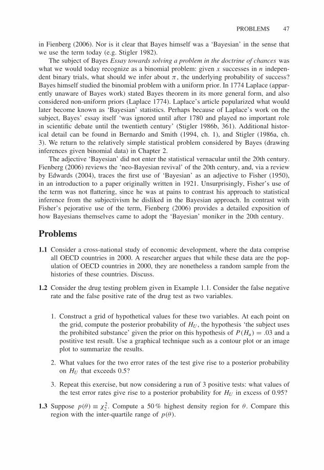
PROBLEMS 47
in Fienberg (2006). Nor is it clear that Bayes himself was a ‘Bayesian’ in the sense thatwe use the term today (e.g. Stigler 1982).
The subject of Bayes Essay towards solving a problem in the doctrine of chances waswhat we would today recognize as a binomial problem: given x successes in n indepen-dent binary trials, what should we infer about π , the underlying probability of success?Bayes himself studied the binomial problem with a uniform prior. In 1774 Laplace (appar-ently unaware of Bayes work) stated Bayes theorem in its more general form, and alsoconsidered non-uniform priors (Laplace 1774). Laplace’s article popularized what wouldlater become known as ‘Bayesian’ statistics. Perhaps because of Laplace’s work on thesubject, Bayes’ essay itself ‘was ignored until after 1780 and played no important rolein scientific debate until the twentieth century’ (Stigler 1986b, 361). Additional histor-ical detail can be found in Bernardo and Smith (1994, ch. 1), and Stigler (1986a, ch.3). We return to the relatively simple statistical problem considered by Bayes (drawinginferences given binomial data) in Chapter 2.
The adjective ‘Bayesian’ did not enter the statistical vernacular until the 20th century.Fienberg (2006) reviews the ‘neo-Bayesian revival’ of the 20th century, and, via a reviewby Edwards (2004), traces the first use of ‘Bayesian’ as an adjective to Fisher (1950),in an introduction to a paper originally written in 1921. Unsurprisingly, Fisher’s use ofthe term was not flattering, since he was at pains to contrast his approach to statisticalinference from the subjectivism he disliked in the Bayesian approach. In contrast withFisher’s pejorative use of the term, Fienberg (2006) provides a detailed exposition ofhow Bayesians themselves came to adopt the ‘Bayesian’ moniker in the 20th century.
Problems
1.1 Consider a cross-national study of economic development, where the data compriseall OECD countries in 2000. A researcher argues that while these data are the pop-ulation of OECD countries in 2000, they are nonetheless a random sample from thehistories of these countries. Discuss.
1.2 Consider the drug testing problem given in Example 1.1. Consider the false negativerate and the false positive rate of the drug test as two variables.
1. Construct a grid of hypothetical values for these two variables. At each point onthe grid, compute the posterior probability of HU , the hypothesis ‘the subject usesthe prohibited substance’ given the prior on this hypothesis of P(Hu) = .03 and apostitive test result. Use a graphical technique such as a contour plot or an imageplot to summarize the results.
2. What values for the two error rates of the test give rise to a posterior probabilityon HU that exceeds 0.5?
3. Repeat this exercise, but now considering a run of 3 positive tests: what values ofthe test error rates give rise to a posterior probability for HU in excess of 0.95?
1.3 Suppose p(θ) ≡ χ22 . Compute a 50 % highest density region for θ . Compare this
region with the inter-quartile range of p(θ).
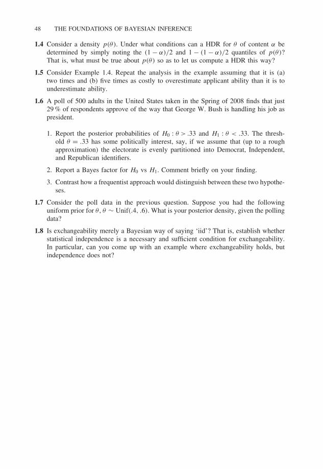
48 THE FOUNDATIONS OF BAYESIAN INFERENCE
1.4 Consider a density p(θ). Under what conditions can a HDR for θ of content α bedetermined by simply noting the (1 − α)/2 and 1 − (1 − α)/2 quantiles of p(θ)?That is, what must be true about p(θ) so as to let us compute a HDR this way?
1.5 Consider Example 1.4. Repeat the analysis in the example assuming that it is (a)two times and (b) five times as costly to overestimate applicant ability than it is tounderestimate ability.
1.6 A poll of 500 adults in the United States taken in the Spring of 2008 finds that just29 % of respondents approve of the way that George W. Bush is handling his job aspresident.
1. Report the posterior probabilities of H0 : θ > .33 and H1 : θ < .33. The thresh-old θ = .33 has some politically interest, say, if we assume that (up to a roughapproximation) the electorate is evenly partitioned into Democrat, Independent,and Republican identifiers.
2. Report a Bayes factor for H0 vs H1. Comment briefly on your finding.
3. Contrast how a frequentist approach would distinguish between these two hypothe-ses.
1.7 Consider the poll data in the previous question. Suppose you had the followinguniform prior for θ , θ ∼ Unif(.4, .6). What is your posterior density, given the pollingdata?
1.8 Is exchangeability merely a Bayesian way of saying ‘iid’? That is, establish whetherstatistical independence is a necessary and sufficient condition for exchangeability.In particular, can you come up with an example where exchangeability holds, butindependence does not?