Analysis of Environmental Data Conceptual Foundations ... · Bayesian inference 2 1. Bayesian parametric inference As we have seen, the method of ordinary least squares can be used

Analysis of Environmental DataConceptual Foundations:

Bay e s ian In fe re n c e

1. Bayesian parametric inference. . . . . . . . . . . . . . . . . . . . . . . . . . . . . . . . . . . . . . . . . . . . . . . . . . . 22. Parameter estimation the Bayesian way. . . . . . . . . . . . . . . . . . . . . . . . . . . . . . . . . . . . . . . . . . . . 33. Credible intervals. . . . . . . . . . . . . . . . . . . . . . . . . . . . . . . . . . . . . . . . . . . . . . . . . . . . . . . . . . . . 274. Model comparison. . . . . . . . . . . . . . . . . . . . . . . . . . . . . . . . . . . . . . . . . . . . . . . . . . . . . . . . . . . 295. Predictions.. . . . . . . . . . . . . . . . . . . . . . . . . . . . . . . . . . . . . . . . . . . . . . . . . . . . . . . . . . . . . . . . . 346. Pros and cons of Bayesian likelihood inference. . . . . . . . . . . . . . . . . . . . . . . . . . . . . . . . . . . . 35

Bayesian inference 2

1. Bayesian parametric inference

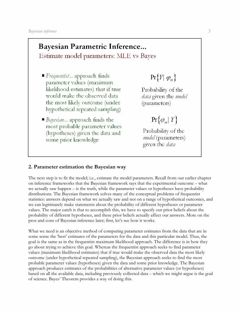
As we have seen, the method of ordinary least squares can be used to find the best fit of a model tothe data under minimal assumptions about the sources of uncertainty and the method of maximumlikelihood can be used to find the best fit of a model the data when we are willing to make certainassumptions about how uncertainty enters into the system. When a parametric approach can bejustified, Bayesian inference offers an alternative to Maximum Likelihood and allows us to determinethe probability of the model (parameters) given the data – something we cannot do with maximumlikelihood. Bayesian inference is especially useful when we want to combine new data with priorknowledge of the system to make inferences that better reflect the cumulative nature of scientificinference.


2. Parameter estimation the Bayesian way

The next step is to fit the model; i.e., estimate the model parameters. Recall from our earlier chapteron inference frameworks that the Bayesian framework says that the experimental outcome – whatwe actually saw happen – is the truth, while the parameter values or hypotheses have probabilitydistributions. The Bayesian framework solves many of the conceptual problems of frequentiststatistics: answers depend on what we actually saw and not on a range of hypothetical outcomes, andwe can legitimately make statements about the probability of different hypotheses or parametervalues. The major catch is that to accomplish this, we have to specify our prior beliefs about theprobability of different hypotheses, and these prior beliefs actually affect our answers. More on thepros and cons of Bayesian inference later; first, let’s see how it works.

What we need is an objective method of computing parameter estimates from the data that are insome sense the ‘best’ estimates of the parameters for the data and this particular model. Thus, thegoal is the same as in the frequentist maximum likelihood approach. The difference is in how theygo about trying to achieve this goal. Whereas the frequentist approach seeks to find parametervalues (maximum likelihood estimates) that if true would make the observed data the most likelyoutcome (under hypothetical repeated sampling), the Bayesian approach seeks to find the mostprobable parameter values (hypotheses) given the data and some prior knowledge. The Bayesianapproach produces estimates of the probabilities of alternative parameter values (or hypotheses)based on all the available data, including previously collected data – which we might argue is the goalof science. Bayes’ Theorem provides a way of doing this.


Conditional Probability:

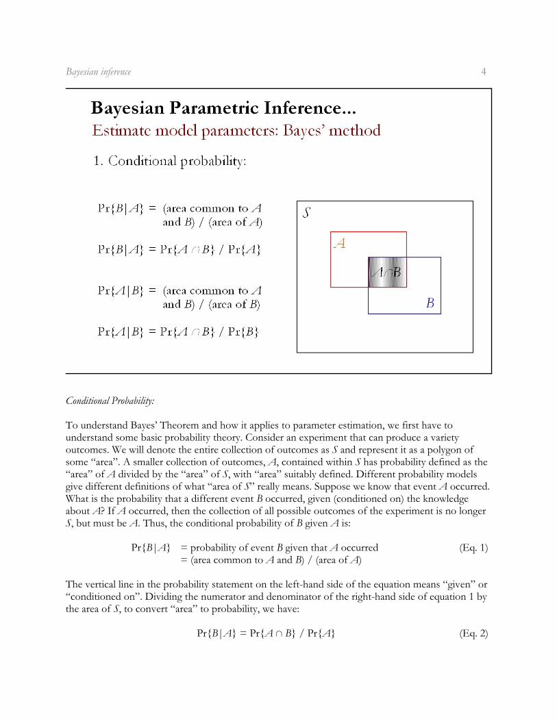
To understand Bayes’ Theorem and how it applies to parameter estimation, we first have tounderstand some basic probability theory. Consider an experiment that can produce a varietyoutcomes. We will denote the entire collection of outcomes as S and represent it as a polygon ofsome “area”. A smaller collection of outcomes, A, contained within S has probability defined as the“area” of A divided by the “area” of S, with “area” suitably defined. Different probability modelsgive different definitions of what “area of S” really means. Suppose we know that event A occurred.What is the probability that a different event B occurred, given (conditioned on) the knowledgeabout A? If A occurred, then the collection of all possible outcomes of the experiment is no longerS, but must be A. Thus, the conditional probability of B given A is:

Pr{B|A} = probability of event B given that A occurred (Eq. 1)= (area common to A and B) / (area of A)

The vertical line in the probability statement on the left-hand side of the equation means “given” or“conditioned on”. Dividing the numerator and denominator of the right-hand side of equation 1 bythe area of S, to convert “area” to probability, we have:

Pr{B|A} = Pr{A 1 B} / Pr{A} (Eq. 2)


where “1 ” stands for “and” or “intersection”. By analogy, since A and B are fully interchangeablehere, we must also have:

Pr{A|B} = Pr{A 1 B} / Pr{B} (Eq. 3)

Equation 3 is how we define “conditional probability”: the probability of something given(conditioned on) something else.


Bayes Theorem:

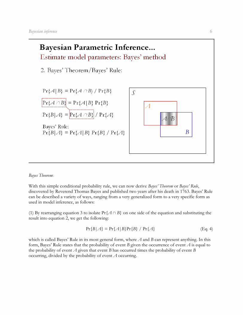
With this simple conditional probability rule, we can now derive Bayes’ Theorem or Bayes’ Rule,discovered by Reverend Thomas Bayes and published two years after his death in 1763. Bayes’ Rulecan be described a variety of ways, ranging from a very generalized form to a very specific form asused in model inference, as follows:

(1) By rearranging equation 3 to isolate Pr{A 1 B} on one side of the equation and substituting theresult into equation 2, we get the following:

Pr{B|A} = Pr{A|B}Pr{B} / Pr{A} (Eq. 4)

which is called Bayes’ Rule in its most general form, where A and B can represent anything. In thisform, Bayes’ Rule states that the probability of event B given the occurrence of event A is equal tothe probability of event A given that event B has occurred times the probability of event Boccurring, divided by the probability of event A occurring.


(2) If we substitute “hypothesis” (or “model”) for B and “data” for A in equation 4, we get thefollowing:

Pr{hypothesis|data} = Pr{data|hypothesis}Pr{hypothesis} / Pr{data}

or simply:

Pr{H|D} = Pr{D|H}Pr{H} / Pr{D} (Eq. 5)

In this context, Bayes’ Rule states that the probability of the hypothesis (parameter values) given thedata is equal to the probability of the data given the hypothesis (the likelihood associated with H),times the probability of the hypothesis, divided by the probability of the data. The left-hand side ofthe equation gives the probability of any particular parameter value(s) given the data.


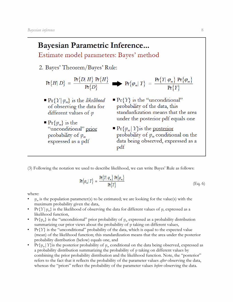
(3) Following the notation we used to describe likelihood, we can write Bayes’ Rule as follows:

(Eq. 6)

where:

m• ö is the population parameter(s) to be estimated; we are looking for the value(s) with themaximum probability given the data,

m• Pr{Y|ö } is the likelihood of observing the data for different values of ö, expressed as alikelihood function,

m m• Pr{ö } is the “unconditional” prior probability of ö expressed as a probability distributionsummarizing our prior views about the probability of ö taking on different values,

• Pr{Y} is the “unconditional” probability of the data, which is equal to the expected value(mean) of the likelihood function; this standardization means that the area under the posteriorprobability distribution (below) equals one, and

m m• Pr{ö |Y}is the posterior probability of ö conditional on the data being observed, expressed asa probability distribution summarizing the probability of ö taking on different values bycombining the prior probability distribution and the likelihood function. Note, the “posterior”refers to the fact that it reflects the probability of the parameter values after observing the data,whereas the “priors” reflect the probability of the parameter values before observing the data.


(4) We can re-express Bayes’ Rule even more simply as follows:

Posterior probability % likelihood x prior probability (Eq. 7)

where “%” means proportional to, because the denominator Pr{Y}in equation 6 is simply anormalizing constant that makes the posterior probability a true probability. Note that likelihood iswhere our data comes in and is the same likelihood we used in maximum likelihood estimation.Thus, the major difference between Bayesian estimation and maximum likelihood estimation iswhether prior knowledge is taken into account.

If Bayes’ Rule seems too good to be true, it’s because it might just be. There are a couple of majorproblems with the application of Bayes’ Rule in statistical inference (that frequentists are keen topoint out): (1) we don’t know the unconditional probability of the data Pr{Y}, and (2) we don’t

mknow the unconditional prior probability of the hypothesis Pr{ö }– isn’t that what we were trying tofigure out in the first place. These problems have received considerable attention among statisticiansand have important implications, so let’s briefly consider each of these problems in turn.


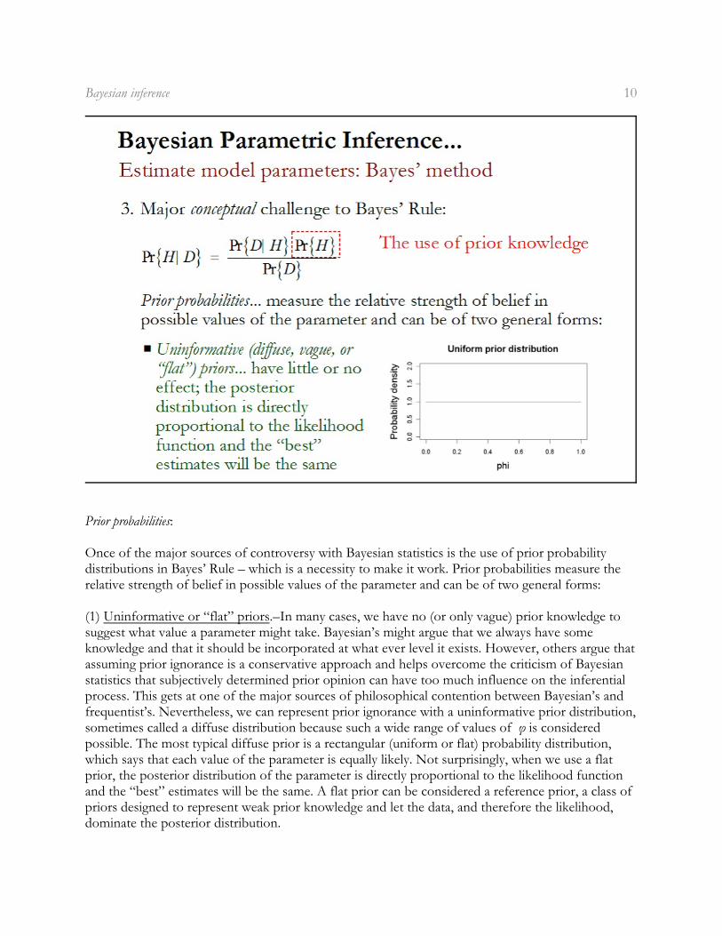
Prior probabilities:

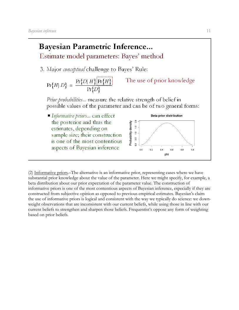
Once of the major sources of controversy with Bayesian statistics is the use of prior probabilitydistributions in Bayes’ Rule – which is a necessity to make it work. Prior probabilities measure therelative strength of belief in possible values of the parameter and can be of two general forms:

(1) Uninformative or “flat” priors.–In many cases, we have no (or only vague) prior knowledge tosuggest what value a parameter might take. Bayesian’s might argue that we always have someknowledge and that it should be incorporated at what ever level it exists. However, others argue thatassuming prior ignorance is a conservative approach and helps overcome the criticism of Bayesianstatistics that subjectively determined prior opinion can have too much influence on the inferentialprocess. This gets at one of the major sources of philosophical contention between Bayesian’s andfrequentist’s. Nevertheless, we can represent prior ignorance with a uninformative prior distribution,sometimes called a diffuse distribution because such a wide range of values of ö is consideredpossible. The most typical diffuse prior is a rectangular (uniform or flat) probability distribution,which says that each value of the parameter is equally likely. Not surprisingly, when we use a flatprior, the posterior distribution of the parameter is directly proportional to the likelihood functionand the “best” estimates will be the same. A flat prior can be considered a reference prior, a class ofpriors designed to represent weak prior knowledge and let the data, and therefore the likelihood,dominate the posterior distribution.


(2) Informative priors.–The alternative is an informative prior, representing cases where we havesubstantial prior knowledge about the value of the parameter. Here we might specify, for example, abeta distribution about our prior expectation of the parameter value. The construction ofinformative priors is one of the most contentious aspects of Bayesian inference, especially if they areconstructed from subjective opinion as opposed to previous empirical estimates. Bayesian’s claimthe use of informative priors is logical and consistent with the way we typically do science: we down-weight observations that are inconsistent with our current beliefs, while using those in line with ourcurrent beliefs to strengthen and sharpen those beliefs. Frequentist’s oppose any form of weightingbased on prior beliefs.


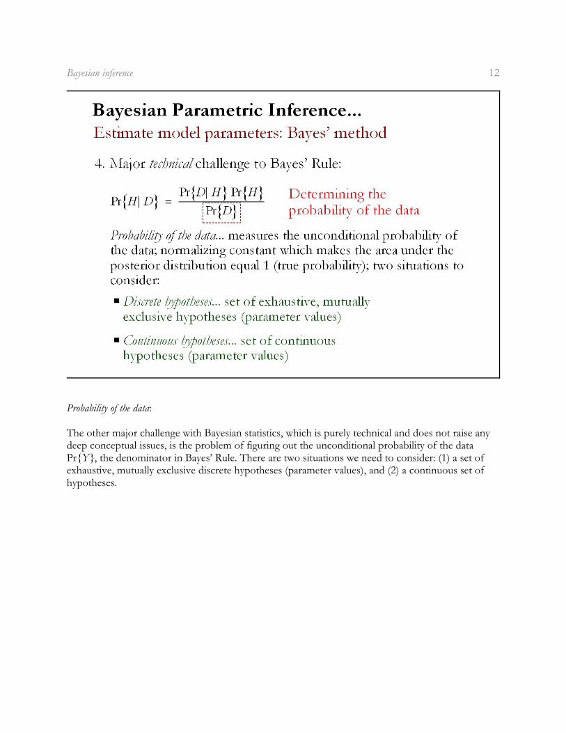
Probability of the data:

The other major challenge with Bayesian statistics, which is purely technical and does not raise anydeep conceptual issues, is the problem of figuring out the unconditional probability of the dataPr{Y}, the denominator in Bayes’ Rule. There are two situations we need to consider: (1) a set ofexhaustive, mutually exclusive discrete hypotheses (parameter values), and (2) a continuous set ofhypotheses.


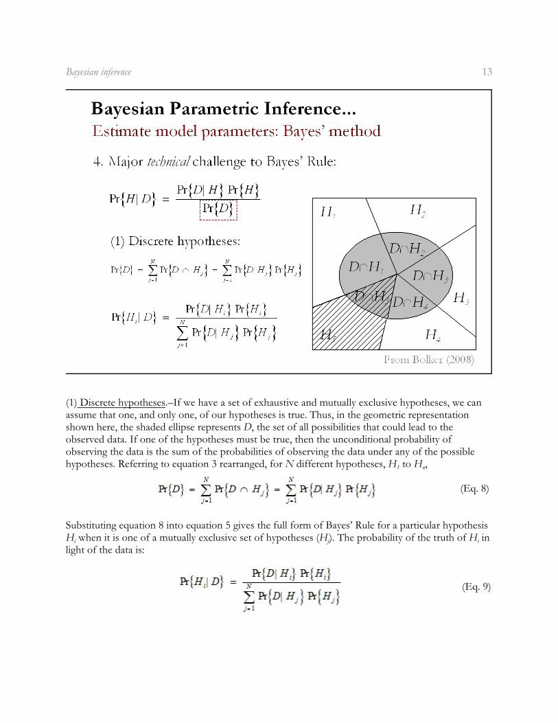
(1) Discrete hypotheses.–If we have a set of exhaustive and mutually exclusive hypotheses, we canassume that one, and only one, of our hypotheses is true. Thus, in the geometric representationshown here, the shaded ellipse represents D, the set of all possibilities that could lead to theobserved data. If one of the hypotheses must be true, then the unconditional probability ofobserving the data is the sum of the probabilities of observing the data under any of the possible

1 nhypotheses. Referring to equation 3 rearranged, for N different hypotheses, H to H ,

(Eq. 8)

Substituting equation 8 into equation 5 gives the full form of Bayes’ Rule for a particular hypothesis

i j iH when it is one of a mutually exclusive set of hypotheses (H ). The probability of the truth of H inlight of the data is:

(Eq. 9)


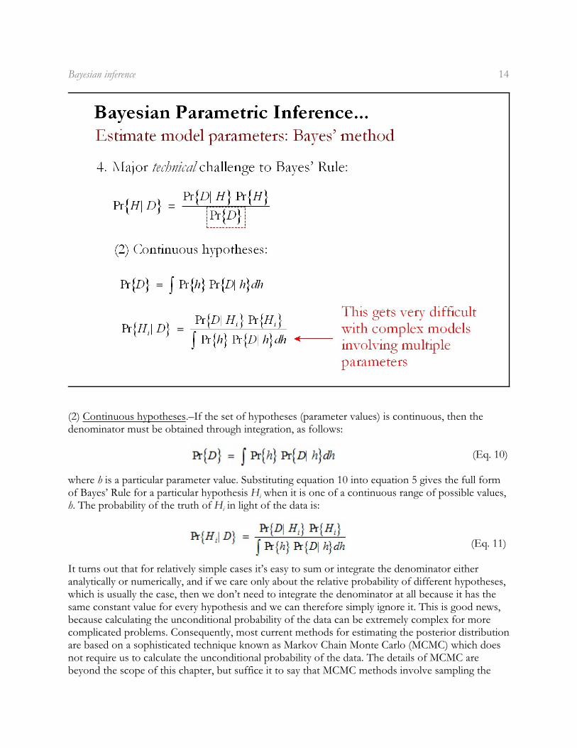
(2) Continuous hypotheses.–If the set of hypotheses (parameter values) is continuous, then thedenominator must be obtained through integration, as follows:

(Eq. 10)

where h is a particular parameter value. Substituting equation 10 into equation 5 gives the full form

iof Bayes’ Rule for a particular hypothesis H when it is one of a continuous range of possible values,

ih. The probability of the truth of H in light of the data is:

(Eq. 11)

It turns out that for relatively simple cases it’s easy to sum or integrate the denominator eitheranalytically or numerically, and if we care only about the relative probability of different hypotheses,which is usually the case, then we don’t need to integrate the denominator at all because it has thesame constant value for every hypothesis and we can therefore simply ignore it. This is good news,because calculating the unconditional probability of the data can be extremely complex for morecomplicated problems. Consequently, most current methods for estimating the posterior distributionare based on a sophisticated technique known as Markov Chain Monte Carlo (MCMC) which doesnot require us to calculate the unconditional probability of the data. The details of MCMC arebeyond the scope of this chapter, but suffice it to say that MCMC methods involve sampling the


posterior distribution many times in order to estimate the posterior distribution, from which we canextract useful summaries such as the mean of the sample posterior distribution.

Posterior probability:

All conclusions from Bayesian inference are based on the posterior probability distribution of theparameter or an estimate of the posterior derived from MCMC sampling. This posterior distributionrepresents our prior probability distribution modified by the current data through the likelihoodfunction. Bayesian inference is usually based on the shape of the posterior distribution, particularlythe range of values over which most of the probability mass occurs. The best estimate of theparameter is usually determined from the mean of the posterior distribution.


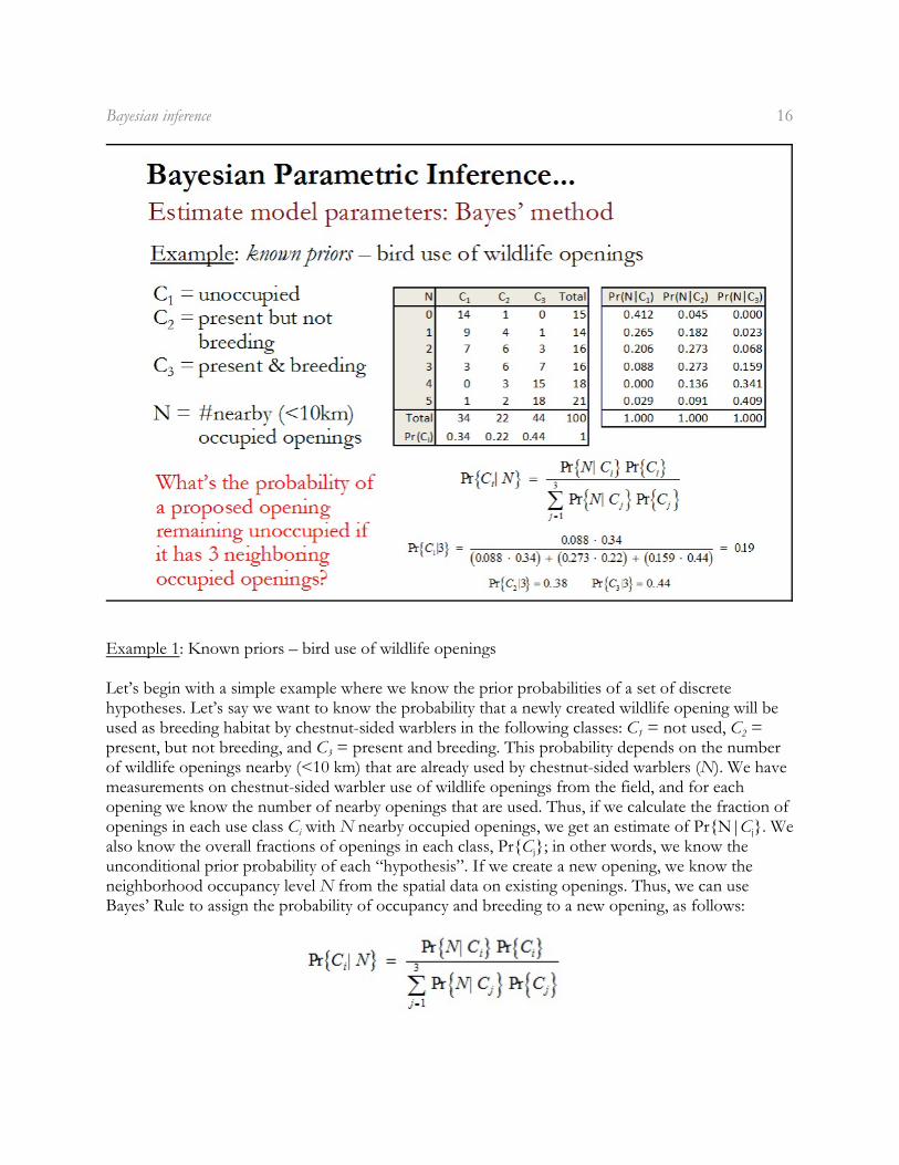
Example 1: Known priors – bird use of wildlife openings

Let’s begin with a simple example where we know the prior probabilities of a set of discretehypotheses. Let’s say we want to know the probability that a newly created wildlife opening will be

1 2used as breeding habitat by chestnut-sided warblers in the following classes: C = not used, C =

3present, but not breeding, and C = present and breeding. This probability depends on the numberof wildlife openings nearby (<10 km) that are already used by chestnut-sided warblers (N). We havemeasurements on chestnut-sided warbler use of wildlife openings from the field, and for eachopening we know the number of nearby openings that are used. Thus, if we calculate the fraction of

i jopenings in each use class C with N nearby occupied openings, we get an estimate of Pr{N|C }. We

jalso know the overall fractions of openings in each class, Pr{C }; in other words, we know theunconditional prior probability of each “hypothesis”. If we create a new opening, we know theneighborhood occupancy level N from the spatial data on existing openings. Thus, we can useBayes’ Rule to assign the probability of occupancy and breeding to a new opening, as follows:


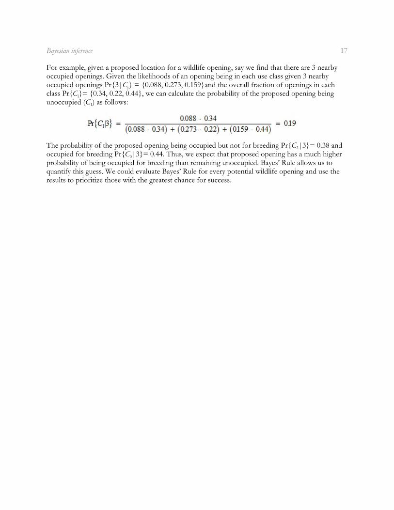
For example, given a proposed location for a wildlife opening, say we find that there are 3 nearbyoccupied openings. Given the likelihoods of an opening being in each use class given 3 nearby

joccupied openings Pr{3|C } = {0.088, 0.273, 0.159}and the overall fraction of openings in each

jclass Pr{C }= {0.34, 0.22, 0.44}, we can calculate the probability of the proposed opening being

1unoccupied (C ) as follows:

2The probability of the proposed opening being occupied but not for breeding Pr{C |3}= 0.38 and

3occupied for breeding Pr{C |3}= 0.44. Thus, we expect that proposed opening has a much higherprobability of being occupied for breeding than remaining unoccupied. Bayes’ Rule allows us toquantify this guess. We could evaluate Bayes’ Rule for every potential wildlife opening and use theresults to prioritize those with the greatest chance for success.


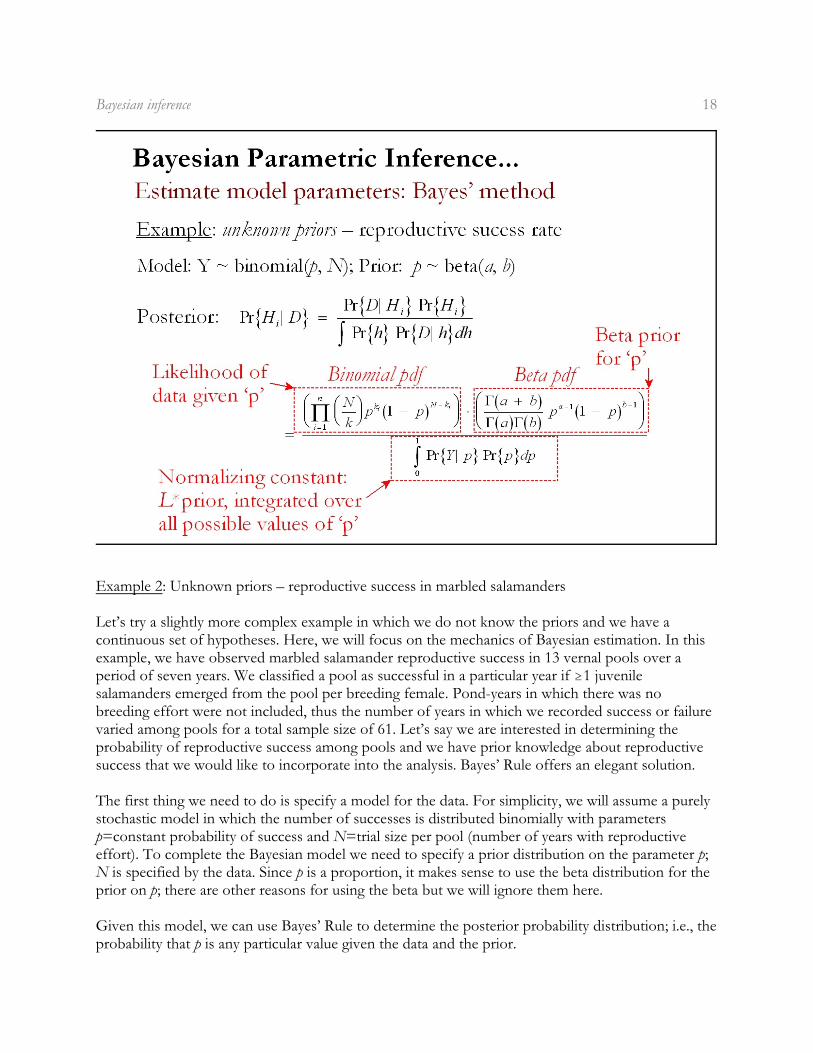
Example 2: Unknown priors – reproductive success in marbled salamanders

Let’s try a slightly more complex example in which we do not know the priors and we have acontinuous set of hypotheses. Here, we will focus on the mechanics of Bayesian estimation. In thisexample, we have observed marbled salamander reproductive success in 13 vernal pools over aperiod of seven years. We classified a pool as successful in a particular year if $1 juvenilesalamanders emerged from the pool per breeding female. Pond-years in which there was nobreeding effort were not included, thus the number of years in which we recorded success or failurevaried among pools for a total sample size of 61. Let’s say we are interested in determining theprobability of reproductive success among pools and we have prior knowledge about reproductivesuccess that we would like to incorporate into the analysis. Bayes’ Rule offers an elegant solution.

The first thing we need to do is specify a model for the data. For simplicity, we will assume a purelystochastic model in which the number of successes is distributed binomially with parametersp=constant probability of success and N=trial size per pool (number of years with reproductiveeffort). To complete the Bayesian model we need to specify a prior distribution on the parameter p;N is specified by the data. Since p is a proportion, it makes sense to use the beta distribution for theprior on p; there are other reasons for using the beta but we will ignore them here.

Given this model, we can use Bayes’ Rule to determine the posterior probability distribution; i.e., theprobability that p is any particular value given the data and the prior.


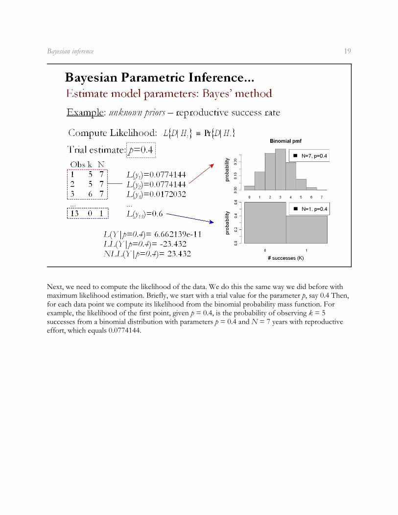
Next, we need to compute the likelihood of the data. We do this the same way we did before withmaximum likelihood estimation. Briefly, we start with a trial value for the parameter p, say 0.4 Then,for each data point we compute its likelihood from the binomial probability mass function. Forexample, the likelihood of the first point, given p = 0.4, is the probability of observing k = 5successes from a binomial distribution with parameters p = 0.4 and N = 7 years with reproductiveeffort, which equals 0.0774144.


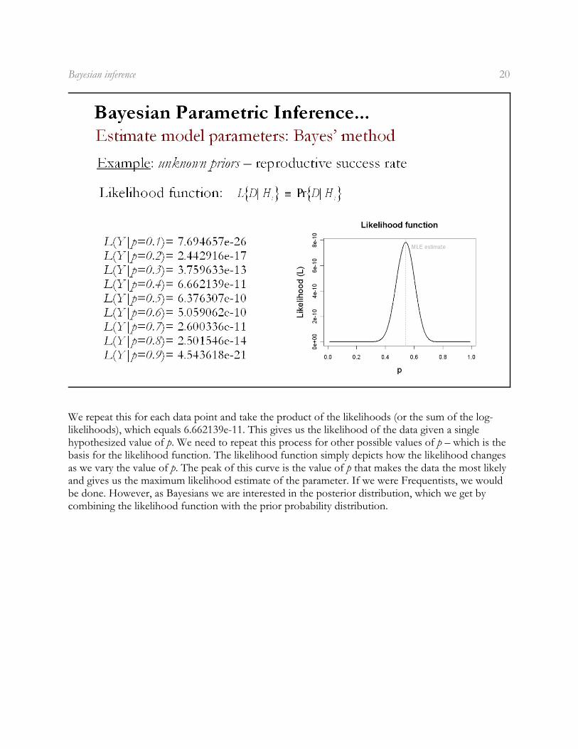
We repeat this for each data point and take the product of the likelihoods (or the sum of the log-likelihoods), which equals 6.662139e-11. This gives us the likelihood of the data given a singlehypothesized value of p. We need to repeat this process for other possible values of p – which is thebasis for the likelihood function. The likelihood function simply depicts how the likelihood changesas we vary the value of p. The peak of this curve is the value of p that makes the data the most likelyand gives us the maximum likelihood estimate of the parameter. If we were Frequentists, we wouldbe done. However, as Bayesians we are interested in the posterior distribution, which we get bycombining the likelihood function with the prior probability distribution.


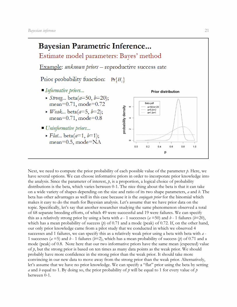
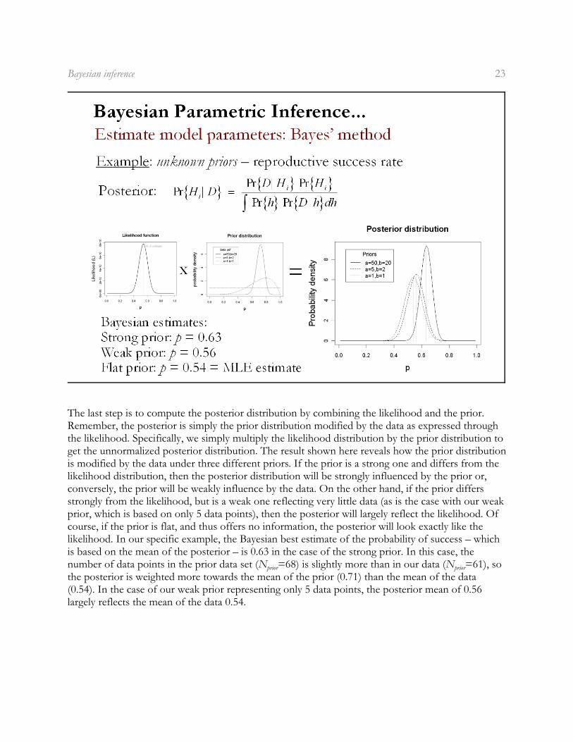
Next, we need to compute the prior probability of each possible value of the parameter p. Here, wehave several options. We can choose informative priors in order to incorporate prior knowledge intothe analysis. Since the parameter of interest, p, is a proportion, a logical choice of probabilitydistributions is the beta, which varies between 0-1. The nice thing about the beta is that it can takeon a wide variety of shapes depending on the size and ratio of its two shape parameters, a and b. Thebeta has other advantages as well in this case because it is the conjugate prior for the binomial whichmakes it easy to do the math for Bayesian analysis. Let’s assume that we have prior data on thetopic. Specifically, let’s say that another researcher studying the same phenomenon observed a totalof 68 separate breeding efforts, of which 49 were successful and 19 were failures. We can specifythis as a relatively strong prior by using a beta with a - 1 successes (a =50) and b - 1 failures (b=20),which has a mean probability of success (p) of 0.71 and a mode (peak) of 0.72. If, on the other hand,our only prior knowledge came from a pilot study that we conducted in which we observed 4successes and 1 failures, we can specify this as a relatively weak prior using a beta with beta with a -1 successes (a =5) and b - 1 failures (b=2), which has a mean probability of success (p) of 0.71 and amode (peak) of 0.8. Note here that our two informative priors have the same mean (expected) valueof p, but the strong prior is based on ten times as many data points as the weak prior. We shouldprobably have more confidence in the strong prior than the weak prior. It should take moreconvincing in our new data to move away from the strong prior than the weak prior. Alternatively,let’s assume that we have no prior knowledge. We can specify a “flat” prior using the beta by settinga and b equal to 1. By doing so, the prior probability of p will be equal to 1 for every value of pbetween 0-1.


Next, to complete the full Bayesian analysis, we need to compute the probability of the data, thedenominator in the Bayes’ equation. This is necessary to make the posterior distribution a trueprobability distribution – area equal to 1. However, it is only sometimes useful to be able to expressthe posterior as a true probability – our first example on wildlife openings was such a case. Moreoften than not, however, we can ignore the denominator because our interest lies in finding the bestestimate of the parameter not in determining its absolute probability. For our purposes, we willsimply ignore the denominator. Calculating the denominator will not change the shape of theposterior distribution at all; it will only change the scale of the y-axis. In simple models like the onewe are considering here, it is actually quite simple to calculate the denominator using either analyticalor numerical integration, but the procedures for doing this go beyond the scope of this chapter.


The last step is to compute the posterior distribution by combining the likelihood and the prior.Remember, the posterior is simply the prior distribution modified by the data as expressed throughthe likelihood. Specifically, we simply multiply the likelihood distribution by the prior distribution toget the unnormalized posterior distribution. The result shown here reveals how the prior distributionis modified by the data under three different priors. If the prior is a strong one and differs from thelikelihood distribution, then the posterior distribution will be strongly influenced by the prior or,conversely, the prior will be weakly influence by the data. On the other hand, if the prior differsstrongly from the likelihood, but is a weak one reflecting very little data (as is the case with our weakprior, which is based on only 5 data points), then the posterior will largely reflect the likelihood. Ofcourse, if the prior is flat, and thus offers no information, the posterior will look exactly like thelikelihood. In our specific example, the Bayesian best estimate of the probability of success – whichis based on the mean of the posterior – is 0.63 in the case of the strong prior. In this case, the

prior priornumber of data points in the prior data set (N =68) is slightly more than in our data (N =61), sothe posterior is weighted more towards the mean of the prior (0.71) than the mean of the data(0.54). In the case of our weak prior representing only 5 data points, the posterior mean of 0.56largely reflects the mean of the data 0.54.


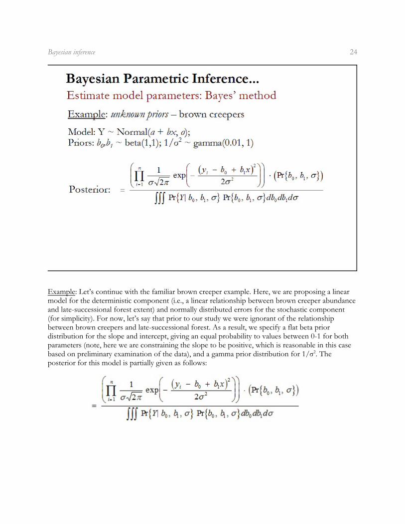
Example: Let’s continue with the familiar brown creeper example. Here, we are proposing a linearmodel for the deterministic component (i.e., a linear relationship between brown creeper abundanceand late-successional forest extent) and normally distributed errors for the stochastic component(for simplicity). For now, let’s say that prior to our study we were ignorant of the relationshipbetween brown creepers and late-successional forest. As a result, we specify a flat beta priordistribution for the slope and intercept, giving an equal probability to values between 0-1 for bothparameters (note, here we are constraining the slope to be positive, which is reasonable in this casebased on preliminary examination of the data), and a gamma prior distribution for 1/ó . The2

posterior for this model is partially given as follows:


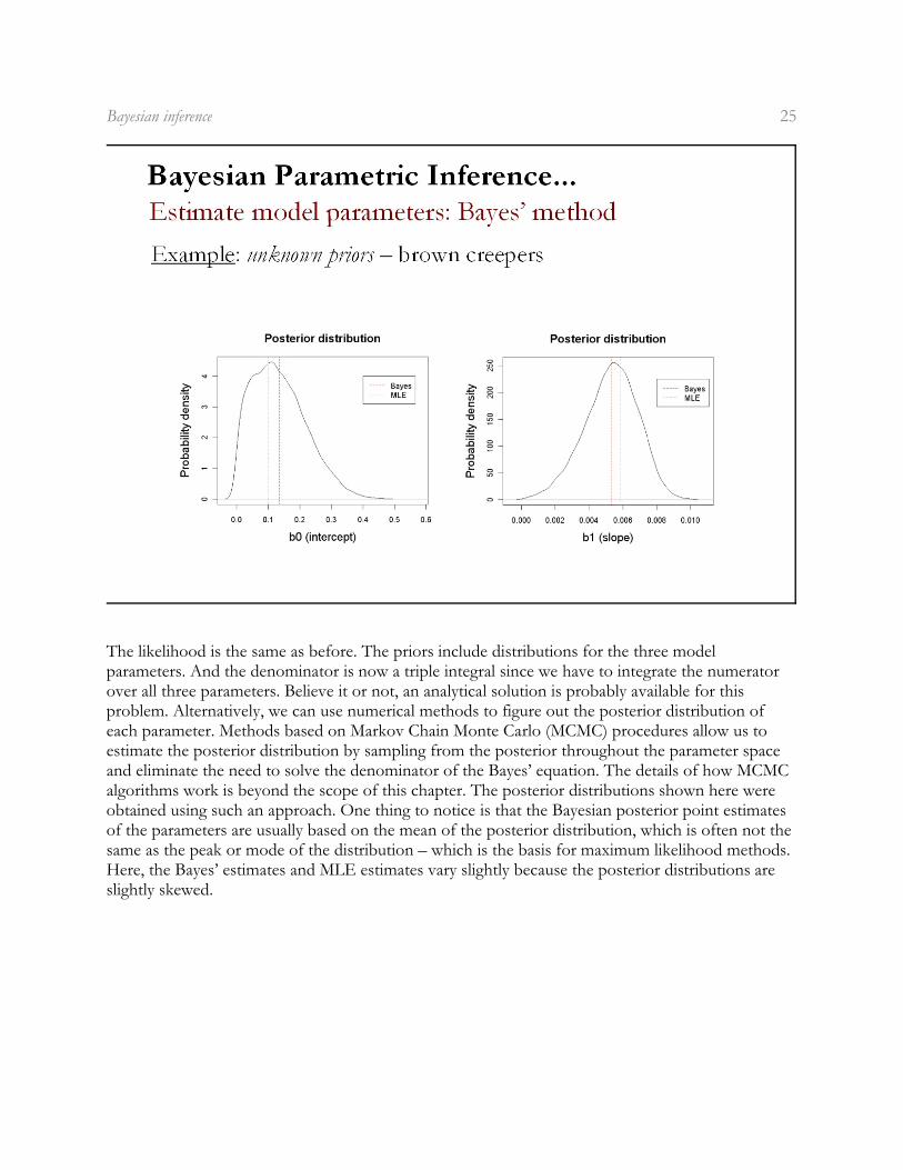
The likelihood is the same as before. The priors include distributions for the three modelparameters. And the denominator is now a triple integral since we have to integrate the numeratorover all three parameters. Believe it or not, an analytical solution is probably available for thisproblem. Alternatively, we can use numerical methods to figure out the posterior distribution ofeach parameter. Methods based on Markov Chain Monte Carlo (MCMC) procedures allow us toestimate the posterior distribution by sampling from the posterior throughout the parameter spaceand eliminate the need to solve the denominator of the Bayes’ equation. The details of how MCMCalgorithms work is beyond the scope of this chapter. The posterior distributions shown here wereobtained using such an approach. One thing to notice is that the Bayesian posterior point estimatesof the parameters are usually based on the mean of the posterior distribution, which is often not thesame as the peak or mode of the distribution – which is the basis for maximum likelihood methods.Here, the Bayes’ estimates and MLE estimates vary slightly because the posterior distributions areslightly skewed.


Pros and cons of Bayesian estimation:

• Bayesian estimation is(typically) a parametricprocedure; thus, it requiresthat we make assumptionsabout the stochasticcomponent of the model;nonparametric Bayesianprocedures exits but are notwidely used as of yet.

• Like maximum likelihoodestimation, Bayesian analysisalso depends on theLikelihood, which can beconstructed for virtually anyproblem.

• With lots of data the choiceof prior won’t matter muchand the parameter estimatesbased on the posteriordistribution will resembleparameter estimates basedon maximum likelihood.

• Regardless of how muchdata we have, we can chooseto carry out an "objective"Bayesian analysis by usinguninformative (vague, flat,diffuse) priors so that thepriors have minimal impacton determining the posteriordistribution and the parameter estimates will resemble those based on maximum likelihood.

• Bayesian estimation based on MCMC methods can be used to obtain parameter estimates fordistributions when it is far too complicated to obtain these estimates using ordinary frequentistoptimization methods; for example, when we are dealing with complex models with manyrandom effects, exotic probability distributions, too many parameters and too little replication.

• However, compared to maximum likelihood estimation conducting Bayesian estimation isextremely complicated and requires considerable technical expertise, even for relatively simplemodels. Thus, it remains to be seen whether Bayesian approaches will ever become mainstreamfor ecologists.


3. Credible intervals

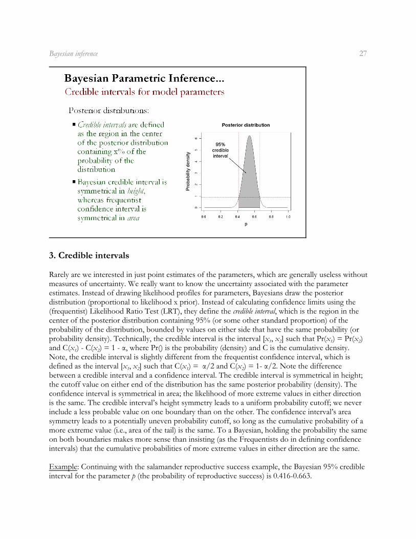
Rarely are we interested in just point estimates of the parameters, which are generally useless withoutmeasures of uncertainty. We really want to know the uncertainty associated with the parameterestimates. Instead of drawing likelihood profiles for parameters, Bayesians draw the posteriordistribution (proportional to likelihood x prior). Instead of calculating confidence limits using the(frequentist) Likelihood Ratio Test (LRT), they define the credible interval, which is the region in thecenter of the posterior distribution containing 95% (or some other standard proportion) of theprobability of the distribution, bounded by values on either side that have the same probability (or

1 2 1 2probability density). Technically, the credible interval is the interval [x , x ] such that Pr(x ) = Pr(x )

1 2and C(x ) - C(x ) = 1 - á, where Pr() is the probability (density) and C is the cumulative density.Note, the credible interval is slightly different from the frequentist confidence interval, which is

1 2 1 2defined as the interval [x , x ] such that C(x ) = á/2 and C(x ) = 1- á/2. Note the differencebetween a credible interval and a confidence interval. The credible interval is symmetrical in height;the cutoff value on either end of the distribution has the same posterior probability (density). Theconfidence interval is symmetrical in area; the likelihood of more extreme values in either directionis the same. The credible interval’s height symmetry leads to a uniform probability cutoff; we neverinclude a less probable value on one boundary than on the other. The confidence interval’s areasymmetry leads to a potentially uneven probability cutoff, so long as the cumulative probability of amore extreme value (i.e., area of the tail) is the same. To a Bayesian, holding the probability the sameon both boundaries makes more sense than insisting (as the Frequentists do in defining confidenceintervals) that the cumulative probabilities of more extreme values in either direction are the same.

Example: Continuing with the salamander reproductive success example, the Bayesian 95% credibleinterval for the parameter p (the probability of reproductive success) is 0.416-0.663.


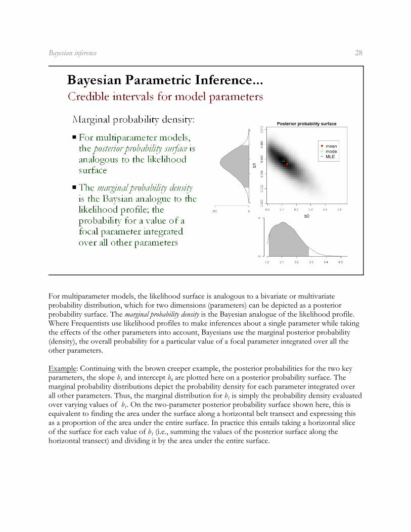
For multiparameter models, the likelihood surface is analogous to a bivariate or multivariateprobability distribution, which for two dimensions (parameters) can be depicted as a posteriorprobability surface. The marginal probability density is the Bayesian analogue of the likelihood profile.Where Frequentists use likelihood profiles to make inferences about a single parameter while takingthe effects of the other parameters into account, Bayesians use the marginal posterior probability(density), the overall probability for a particular value of a focal parameter integrated over all theother parameters.

Example: Continuing with the brown creeper example, the posterior probabilities for the two key

1 0parameters, the slope b and intercept b are plotted here on a posterior probability surface. Themarginal probability distributions depict the probability density for each parameter integrated over

1all other parameters. Thus, the marginal distribution for b is simply the probability density evaluated

1over varying values of b . On the two-parameter posterior probability surface shown here, this isequivalent to finding the area under the surface along a horizontal belt transect and expressing thisas a proportion of the area under the entire surface. In practice this entails taking a horizontal slice

1of the surface for each value of b (i.e., summing the values of the posterior surface along thehorizontal transect) and dividing it by the area under the entire surface.


4. Model comparison

Bayesians generally have no interest in hypothesis testing (although it can be done in the Bayesianframework) and little interest in formal methods of model selection. Dropping a variable from amodel is often equivalent to testing a null hypothesis that the parameter is exactly zero, andBayesians consider such point null hypotheses silly. They would describe a parameter’s distribution asbeing concentrated near zero rather than saying its value is exactly zero. Nevertheless, Bayesians docompute the relative probability of different models, in a way that implicitly recognizes the bias-variance trade-off and penalizes more complex models. Bayesians prefer to make inferences basedon averages rather than on the most likely values; for example, they generally use the posterior meanvalues of parameters rather than the posterior mode. This preference extends to model selection.


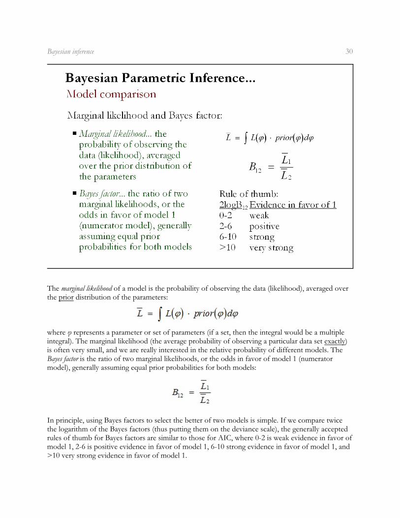
The marginal likelihood of a model is the probability of observing the data (likelihood), averaged overthe prior distribution of the parameters:

where ö represents a parameter or set of parameters (if a set, then the integral would be a multipleintegral). The marginal likelihood (the average probability of observing a particular data set exactly)is often very small, and we are really interested in the relative probability of different models. TheBayes factor is the ratio of two marginal likelihoods, or the odds in favor of model 1 (numeratormodel), generally assuming equal prior probabilities for both models:

In principle, using Bayes factors to select the better of two models is simple. If we compare twicethe logarithm of the Bayes factors (thus putting them on the deviance scale), the generally acceptedrules of thumb for Bayes factors are similar to those for AIC, where 0-2 is weak evidence in favor ofmodel 1, 2-6 is positive evidence in favor of model 1, 6-10 strong evidence in favor of model 1, and>10 very strong evidence in favor of model 1.


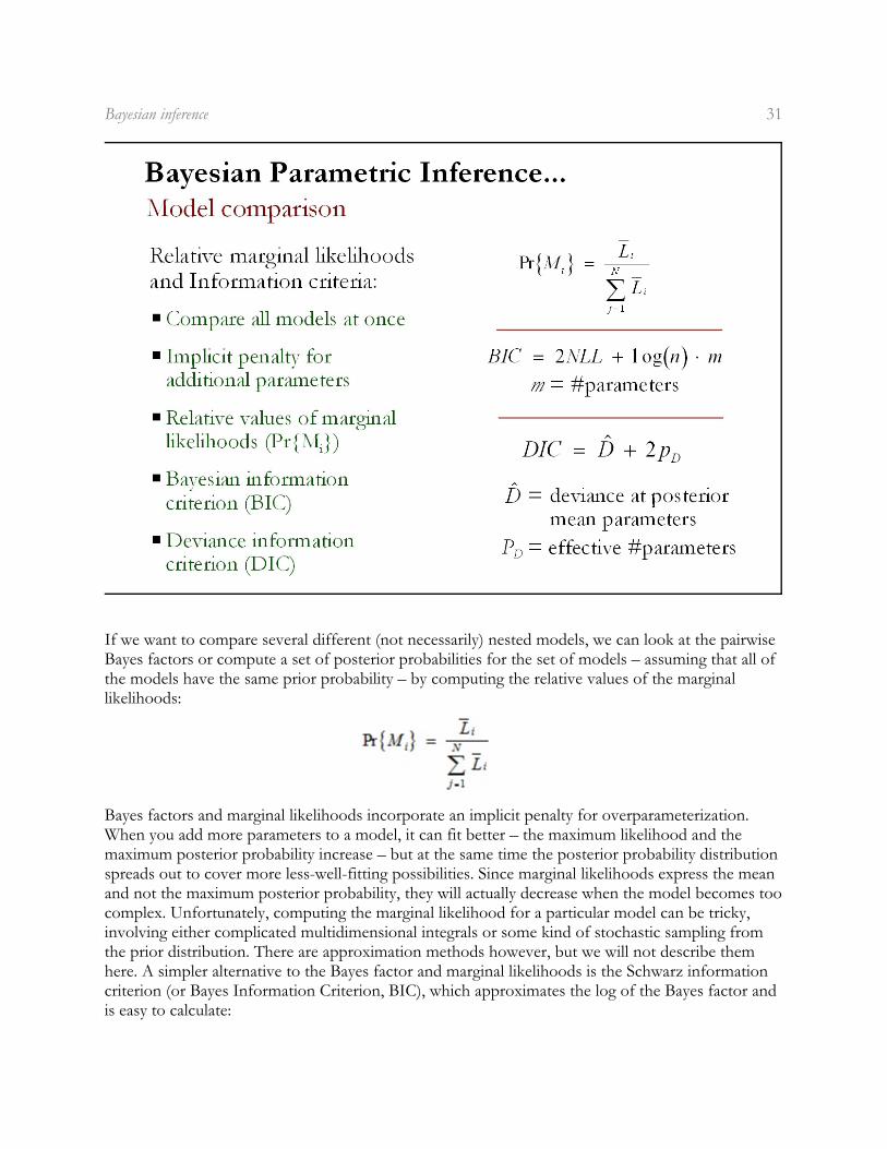
If we want to compare several different (not necessarily) nested models, we can look at the pairwiseBayes factors or compute a set of posterior probabilities for the set of models – assuming that all ofthe models have the same prior probability – by computing the relative values of the marginallikelihoods:

Bayes factors and marginal likelihoods incorporate an implicit penalty for overparameterization.When you add more parameters to a model, it can fit better – the maximum likelihood and themaximum posterior probability increase – but at the same time the posterior probability distributionspreads out to cover more less-well-fitting possibilities. Since marginal likelihoods express the meanand not the maximum posterior probability, they will actually decrease when the model becomes toocomplex. Unfortunately, computing the marginal likelihood for a particular model can be tricky,involving either complicated multidimensional integrals or some kind of stochastic sampling fromthe prior distribution. There are approximation methods however, but we will not describe themhere. A simpler alternative to the Bayes factor and marginal likelihoods is the Schwarz informationcriterion (or Bayes Information Criterion, BIC), which approximates the log of the Bayes factor andis easy to calculate:


where n is the number of observations and m is the number of parameters. When n is greater than e2

. 8 observations (so that log n > 2), the BIC is more conservative than the AIC, insisting on agreater improvement in fit before it will accept a more complex model. Note, while the BIC isderived from a Bayesian argument, it is not inherently a Bayesian technique. Nevertheless, it iscommonly used and reported as such.

A more recent criterion is the DIC, or deviance information criterion, which is similar in concept to AIC – penalized goodness-of-fit – only the goodness-of-fit metric is based on deviance instead ofthe negative log-likelihood:

Dwhere D hat is the deviance calculated at the posterior mean parameters and p is an estimate of theeffective number of parameters.


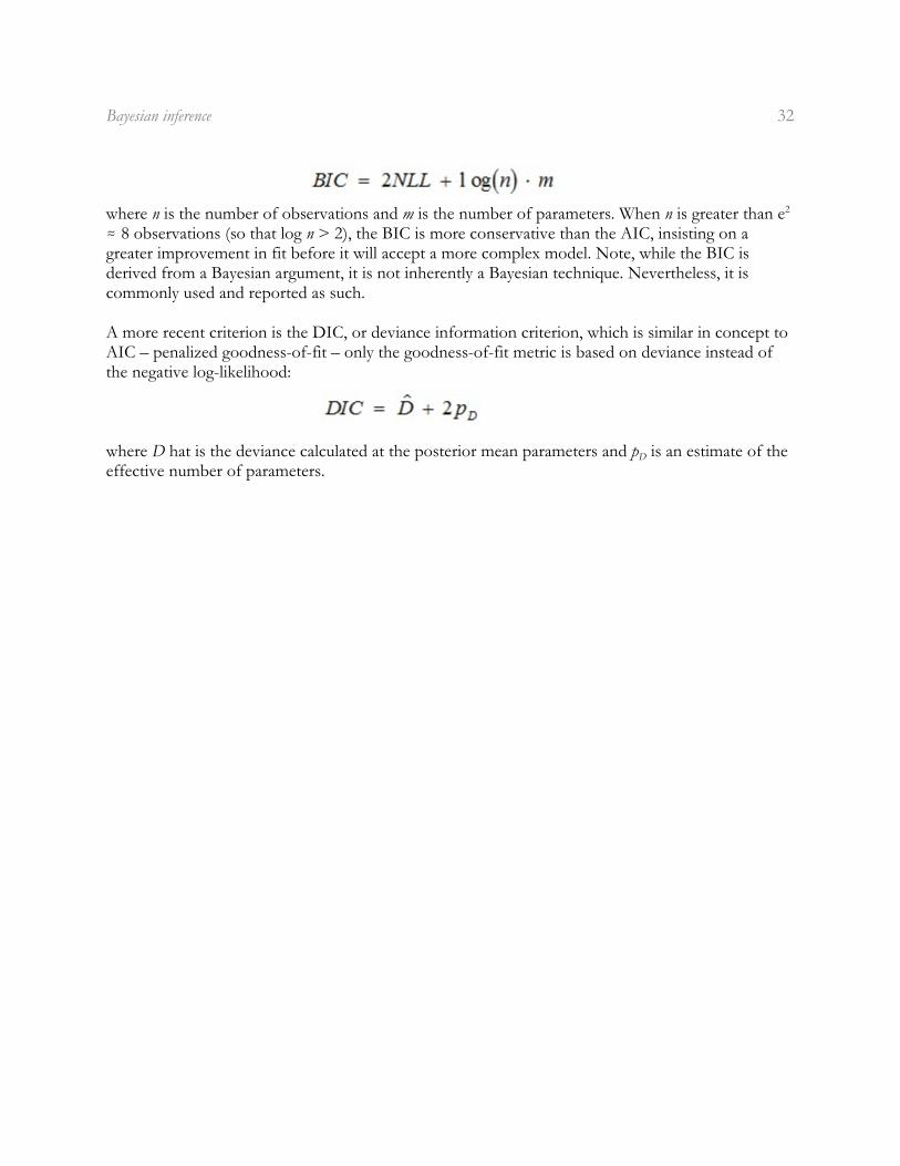
The information criteria such as BIC and DIC are useful for comparing multiple models all at onceand are not suitable for hypotheses testing – which is in line with Bayesian philosophy. Like allinformation criteria, e.g., AIC, BIC and DIC have a general rule of thumb for their interpretation.Differences <5 are considered equivalent, 5-10 distinguishable, and >10 definitely different. Thus,they provide a quick and useful way to compare the weight of evidence in favor of alternativemodels. Indeed, model weights can be calculated from the IC values which give the relativelikelihood or probability of a model given the data. Unfortunately, delving into these measures further is beyond the scope of this chapter and beyondmy complete understanding. Suffice it to say that there are several methods for comparing models ina Bayesian framework, but the tradeoffs among approaches is still being hotly debated.

Example: Continuing with the brown creeper example, recall the three alternative models weconsidered in the maximum likelihood setting. Recall that based on AIC, model 3 was selected asthe “best” model based, with model 1 and 2 close behind. BIC gives model 1 the most weight withmodel 3 and 2 close behind. DIC gives a similar ranking. Not surprisingly, both BIC and DIC weremore conservative than AIC and chose model 1 over the more complex model 3.


5. Predictions

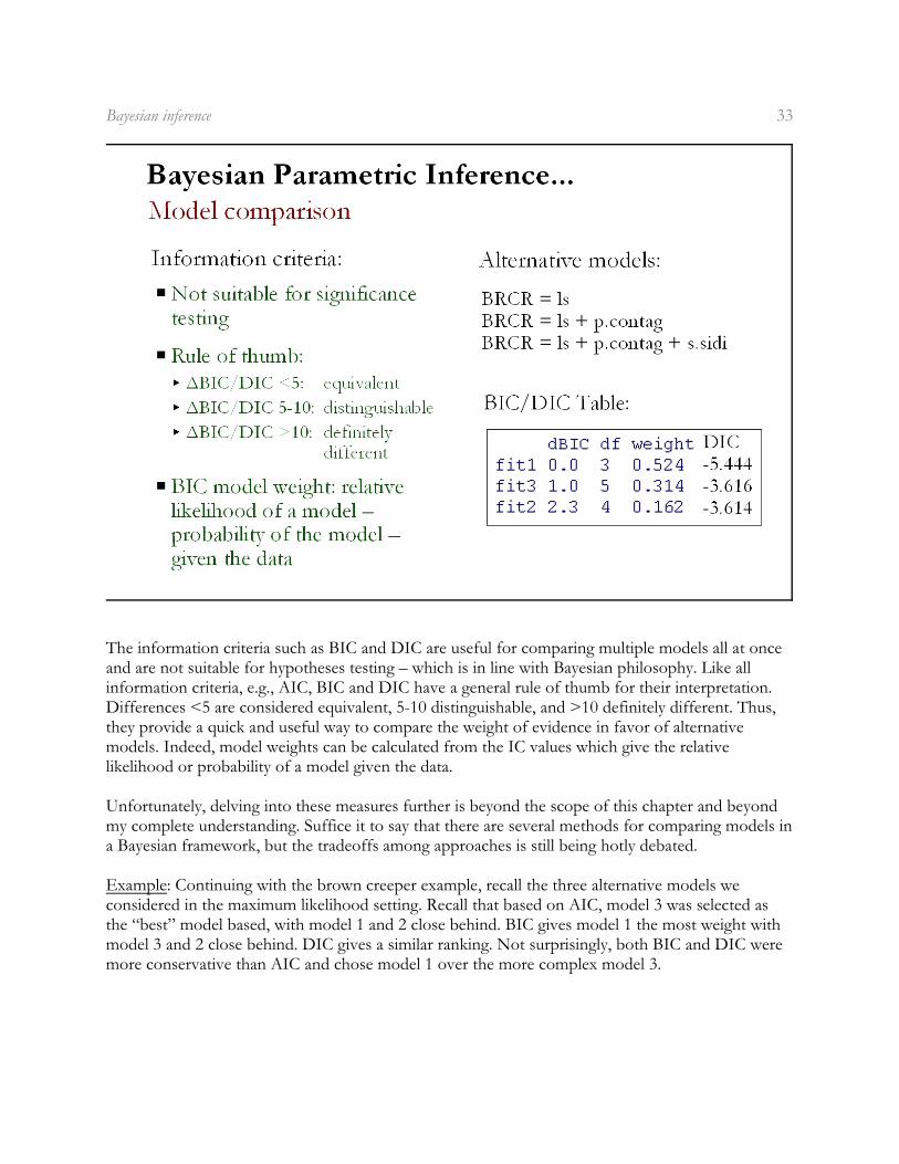
The final goal of statistical inference is to make predictions. In many cases, once we confirm thatour model is a good one, say by confirming that it is significantly better than the null model (e.g., of no relationship between x and y) or that it is the best among competing models considered, wemight want to use this model to predict values for future observations or for sites not sampled.

Unfortunately, I know next to nothing about model predictions in a Bayesian framework. Predictionis certainly doable in the Bayesian framework, but the methods are not familiar to me. So we willskip this topic, but recognize that prediction is possible in a Bayesian framework.


6. Pros and cons of Bayesian likelihood inference

The frequentist Bayesian inference framework is hugely appealing in many respects but it is notwithout some serious drawbacks. We already touched base on many of the pros and cons ofBayesian inference in the section on estimation. Here we will finish with a few additionaloverarching thoughts.

1. Philosophy... Bayesian inference is as much a philosophy as a method. Its distinctiveness arises asmuch from its philosophical underpinnings as the uniqueness of the methods themselves.

2. Technical challenges... Despite the many conceptual advantages of Bayesian statistics, the methodsfor estimation are largely still too complex and technically challenging for mainstream ecology. Itremains to be seen whether enough progress is made in facilitating Bayesian analysis to make itaccessible to vast major of ecologists. Until then, Baysian statistics will likely remain out of reachfor most individuals not willing or able to delve into the gory details of Bayesian anlayticalmethods.

3. Modern statistical inference... Without question Bayesian statistics is the current buzz in ecologicalmodeling and gaining rapidly in popularity over maximum likelihood. However, for the reasonsmentioned above it remains to be seen whether it will end up being a temporary fad or persist.

Documents

Analysis of Environmental Data Conceptual Foundations ... · Bayesian inference 2 1. Bayesian parametric inference As we have seen, the method of ordinary least squares can be used