The Flow Regime of Function: Influence of Flow Changes

on Biogeochemical Processes in Streams

Brynn O’Donnell

Thesis submitted to the faculty of the Virginia Polytechnic Institute and State University

in partial fulfillment of the requirements for the degree of

Master of Science

In

Biological Sciences

Erin R. Hotchkiss, Committee Chair

John E. Barrett

Daniel L. McLaughlin

May 3rd, 2019

Blacksburg, Virginia

Keywords: Disturbance, Stream Metabolism, Flow, Resistance, Resilience

Copyright 2019

The Flow Regime of Function: Influence of Flow Changes

on Biogeochemical Processes in Streams

Brynn O’Donnell

ABSTRACT

Streams are ecosystems organized by disturbance. One of the most frequent disturbances

within a stream is elevated flow. Elevated flow can both stimulate ecosystem processes

and impede them. Consequently, flow plays a critical role in shifting the dominant stream

function between biological transformation and physical transportation of materials. To

garner further insight into the complex interactions of stream function and flow, I

assessed the influence of elevated flow and flow disturbances on stream metabolism. To

do so, I analyzed five years of dissolved oxygen data from an urban- and agriculturally-

influenced stream to estimate metabolism. Stream metabolism is estimated from the

production (gross primary production; GPP) and consumption (ecosystem respiration;

ER) of dissolved oxygen. With these data, I evaluated how low and elevated flows

differentially impact water quality (e.g., turbidity, conductivity) and metabolism using

segmented metabolism- and concentration- discharge analyses. I found that GPP declined

at varying rates across discharge, and ER decreased at lower flows but became constant

at higher flows. Net ecosystem production (NEP; = GPP - ER) reflected the divergence of

GPP and ER and was unchanging at lower flows, but declined at higher discharge. These

C-Q patterns can consequently influence or be influenced by changes in metabolism. I

coupled metabolism-Q and C-Q trends to examine linked flow-induced changes to

physicochemical parameters and metabolism. Parameters related to metabolism (e.g.,

turbidity and GPP, pH and NEP) frequently followed coupled trends. To investigate

metabolic recovery dynamics (i.e., resistance and resilience) following flow disturbances,

I analyzed metabolic responses to 15 isolated flow events and identified the antecedent

conditions or disturbance characteristics that most contributed to recovery dynamics. ER

was both more resistant and resilient than GPP. GPP took longer to recover (1 to >9 days,

mean = 2.5) than ER (1 to 2 days, mean = 1.1). ER resistance was strongly correlated

with the intensity of the flow event, whereas GPP was not, suggesting that GPP responds

similarly to flow disturbances, regardless of the magnitude of flow event. Flow may be

the most frequent disturbance experienced by streams. However, streams are exposed to a

multitude of other disturbances; here I also highlight how anthropogenic alterations to

streams – namely, burying a stream underground – can change biogeochemical function.

This thesis proposes novel frameworks to explore the nexus of flow, anthropogenic

disturbances, and stream function, and thereby to further our understanding of the

complex relationship between streams and disturbances.

The Flow Regime of Function: Influence of Flow Changes

on Biogeochemical Processes in Streams

Brynn O’Donnell

GENERAL AUDIENCE ABSTRACT

A stream is defined by its flowing water. Flow brings the nutrients, organic matter, and

other materials necessary to the algae and bacteria within the stream as well as the

invertebrates and fishes they sustain, and is consequently integral to in-stream biology

and ecology. However, elevated flow is also one of the most frequent disturbances

experienced by streams. Elevated flow dilutes or enriches concentrations of water quality

parameters, moves the water faster, reduces the amount of time essential nutrients are

available to organisms within streams, and scours the algae and bacteria on stream

bottoms. Here, I analyzed five years of data from an urban- and agriculturally-influenced

stream and estimated stream metabolism to explore the influence of flow on stream

biology, chemistry, and ecology. Stream metabolism is a process that reflects the

respiration and photosynthesis of bacteria and algae, estimated from the production and

consumption of dissolved oxygen. The primary research objective of my thesis was to

investigate how changing flow impacts metabolism, by: (1) examining how low and high

flows impact metabolism differently, and (2) studying the response and recovery of

metabolism following multiple flow disturbances. Flow not only influences in-stream

biology and processes, such as stream metabolism, but also changes the water quality of

the stream (e.g., conductivity, pH, turbidity). To examine the interconnection between

flow-induced changes to water quality parameters and metabolism, I measured how low

and high flows impacted water quality and then compared water quality-flow

relationships with metabolism at low and high flows. I found that metabolic processes

and related water quality parameters were frequently coupled. Next, to test how water

quality might also influence the response and recovery of metabolism after a flow

disturbance, I examined whether prior environmental conditions (e.g., temperature, light)

or the magnitude of the flow disturbance influenced metabolic response and recovery. I

found that the size of the flow disturbance did change a critical piece of stream

metabolism. Flow is not the only prevalent disturbance streams face: increasingly,

streams are being altered by ongoing urban and suburbanization. Therefore, to highlight

the full suite of disturbances to streams caused by human modification, I wrote a public

science communication piece documenting the biological, chemical, and ecological

ramifications of burying streams underground. Ultimately, this thesis proposes new

frameworks to more adequately explore the complex relationships between water quality,

stream ecology, and disturbances.

iv

Acknowledgements

I would like to thank my advisor, Dr. Erin Hotchkiss, my committee members, all of Stream

Team, fellow students, and friends for their support these past two years. I must also

acknowledge Bobbie Niederlehner for her unwavering patience with analytical machines. A

special shout-out to Stephen Plont; starting graduate school at the same time as you has been a

blessing. Thank you to the undergraduates who have worked with me in the field and lab, and

shown me what a pleasure it is to mentor.

This research would not exist without Virginia Tech’s StREAM Lab, funded by the VT-

Biological Systems Engineering for baseline StREAM Lab maintenance and monitoring. Cully

Hession generously shared his database and knowledge of our study site, and Laura Lehmann

kindly helped with database access and methods questions.

As always, the biggest thank you of all to my parents, Laurel and Jack, who will not ever read

this far into this thesis and may not even open the e-mail attachment I send them, but without

whom none of it would have been possible.

v

Contents

Chapter One: General Introduction ..................................................................................... 1

References ....................................................................................................................... 8

Chapter Two: Biogeochemical Consequences of Stream Flow Variation: Coupling

Concentration- and Metabolism-Discharge Relationships ............................................... 11

Abstract ......................................................................................................................... 11 Plain Language Summary ............................................................................................. 12 1 Introduction ................................................................................................................ 12

2 Materials and Methods ............................................................................................... 17 3 Results ........................................................................................................................ 23 4 Discussion .................................................................................................................. 31

References ..................................................................................................................... 39 Chapter Three: Resistance and resilience of stream metabolism to high flow disturbances44

Abstract ......................................................................................................................... 44

1 Introduction ................................................................................................................ 45 2 Methods...................................................................................................................... 50

3 Results ........................................................................................................................ 57 4 Discussion .................................................................................................................. 68 References ..................................................................................................................... 77

Chapter Four: 'Ghost streams' sound supernatural, but their impact on your health is very real’

........................................................................................................................................... 81

Chapter Five: General Discussion: Integrating disturbance into our current understanding of

metabolism and stream health ........................................................................................... 87

References ..................................................................................................................... 94

Appendix ........................................................................................................................... 96

Supplement Chapter 1 ................................................................................................... 96

Supplement Chapter 2 ................................................................................................. 106

1

Chapter One: General Introduction

Stream ecosystem scientists were lured by the elusive notion of ecosystem stability for

decades (Webster et al. 1975) and yet, empirical evidence of a stable natural ecosystem evaded

them. Consequently, in the mid-1980s, they began to embrace the innate pulsing nature of

ecosystems, adopting the idea of a pulsing steady state or a pulsing equilibrium in running waters

(Odum et al. 1995, Stanley et al. 2010). As more stochastic, nonequilibrium views of ecosystem

dynamics became more common, the importance of disturbance as a driver of patterns and

conditions of stream processes became quite clear (Resh et al. 1988, Stanley et al. 2010). Here, I

adopt the biological definition of disturbance from White and Pickett (1985): “any relatively

discrete event in time that disrupts the ecosystem… and changes resources, substrate availability,

or the physical environment”. Much of the early work on stream disturbance centered on floods,

but has since expanded to include such aspects as increased nutrient loading, geomorphic

alterations, physical disturbances, or shifts in upstream land use (Stanley et. al. 2010). Two

predominant and interrelated disturbances to stream ecosystems are anthropogenic alterations

and flow.

Flow is integral to the life within a stream, yet also has the potential to impede biotic

function. In fact, Odum et. al (1979) proposed a framework to explain how disturbances, such as

elevated flow, act upon ecosystems across a “subsidy-stress” gradient. Flow drives stream

processes by replenishing resources for microbial activity via distribution of inputs from the

terrestrial environment and upstream, such as nutrients, organic matter, and other chemical

constituents (e.g., Lamberti & Steinman 1997). However, elevated flow is arguably one of the

most predominant disturbances within a stream. Elevated flow can have a replenishing,

subsidizing influence on stream microbial processes (e.g., Beaulieu et al. 2013; Roley et al.

2

2014) or an inhibiting, scouring impact (e.g., Uehlinger 2000, 2006). The disturbance effects of

elevated flow (e.g., scour, altered water quality parameters) can alter internal microbial activity,

and consequently ecosystem function (e.g., Blaszczak et al. 2018). However, flow is frequently

oscillating, and so the balance between its subsidizing or stressing role is constantly shifting back

and forth (Figure 1). The subsidy-stress idea proposed by Odum et al. (1979) was not necessarily

created to describe the relationship between elevated flow and stream ecosystem processes, yet

no other concept describes their interaction so aptly.

Elevated flow can not only subsidize or stress an ecosystem, but can also shift dominant

stream function from the transformation of solutes, including nutrients and organic matter, to

transportation of these solutes (Cole et al. 2007). As a dominant transformer, when stream

processes are ‘normal’ or subsidized by flow (Fig. 1), stream biota have more ‘biophysical

opportunities’ to transform nitrogen, carbon, and other chemical constituents (Battin et al. 2008).

When flow becomes more stressing, dominant stream function can shift to transportation (Fig

1.), sending more solutes to downstream ecosystems as the transformative capabilities of stream

biota are stunted (Raymond et al. 2016). Ultimately, the subsidy-stress and transformer-

transporter frameworks are intricately connected, but are not frequently linked in ecosystem

research.

3

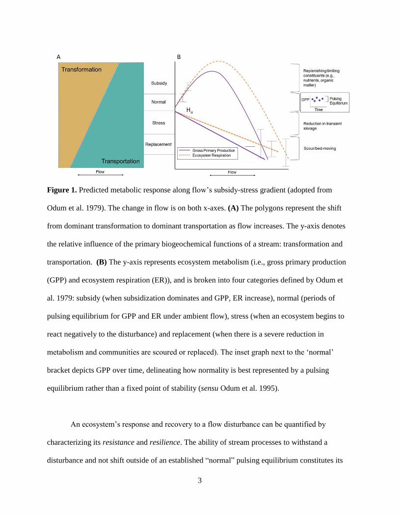
Figure 1. Predicted metabolic response along flow’s subsidy-stress gradient (adopted from

Odum et al. 1979). The change in flow is on both x-axes. (A) The polygons represent the shift

from dominant transformation to dominant transportation as flow increases. The y-axis denotes

the relative influence of the primary biogeochemical functions of a stream: transformation and

transportation. (B) The y-axis represents ecosystem metabolism (i.e., gross primary production

(GPP) and ecosystem respiration (ER)), and is broken into four categories defined by Odum et

al. 1979: subsidy (when subsidization dominates and GPP, ER increase), normal (periods of

pulsing equilibrium for GPP and ER under ambient flow), stress (when an ecosystem begins to

react negatively to the disturbance) and replacement (when there is a severe reduction in

metabolism and communities are scoured or replaced). The inset graph next to the ‘normal’

bracket depicts GPP over time, delineating how normality is best represented by a pulsing

equilibrium rather than a fixed point of stability (sensu Odum et al. 1995).

An ecosystem’s response and recovery to a flow disturbance can be quantified by

characterizing its resistance and resilience. The ability of stream processes to withstand a

disturbance and not shift outside of an established “normal” pulsing equilibrium constitutes its

4

resistance (Figure 1). Resilience is the speed at which an ecosystem returns to this pulsing

equilibrium following a disturbance (Carpenter et al. 1992). Streams are especially vulnerable to

disturbances because they are restricted in their ability to retain material: water is constantly

flowing, carrying contents downstream. However, flow is also a driver of the high resilience of

stream processes. The positive, subsidizing effects of lower flows contribute to the high

resilience of stream processes in the face of disturbances because the unidirectional flow of water

replenishes internal processes (Acuña et al. 2007, Stanley et al. 2010).

Stream metabolism is one of the ecosystem processes that appears to exhibit low

resistance and high resilience to flow disturbances (Uehlinger and Naegeli 1998, Reisinger et al.

2017). Stream metabolism is the biologic production and consumption of dissolved oxygen (e.g.,

gross primary production (GPP) and ecosystem respiration (ER), respectively), through coupled

CO2 fixation (GPP) and organic matter respiration (ER). Net ecosystem production (NEP) is the

balance between GPP and ER. The use of metabolism (GPP, ER, NEP) as an indicator of stream

health (Fellows et al. 2006; Young et al. 2008) and response to disturbances (Arroita et al. 2019)

has increased. Additionally, metabolism is intimately connected to other ecosystem processes,

such as nitrogen uptake (Hall & Tank 2003; Hoellein et al. 2007) and food web dynamics

(Marcarelli et al. 2011). Seasonality drives annual trends of metabolism, but the frequency of

flow disturbances generates smaller time-scale variation (e.g., Uehlinger 2006, Beaulieu et al.

2013; Bernhardt et al. 2018). To recognize trends in metabolism and interpret the flow-induced

variation, we must develop a deeper understanding of metabolic responses to flow disturbances

(Larsen and Harvey 2017, Bernhardt et al. 2018). To explore the connection between metabolism

and flow, I used five years of high-frequency sensor data from a flashy stream (steep rising and

falling limb of a hydrograph shortly after a rain event) draining mixed urban-agricultural land

5

use. I estimated GPP, ER, and NEP to evaluate metabolic response to changing flow, and related

these responses to water quality parameters and antecedent conditions across five years as well

as within isolated flow events.

Low and high flows can impact metabolism and water quality differently. Interactions

between elevated flows and water chemistry (e.g., pH, conductivity, turbidity) are often analyzed

via concentration-discharge (C-Q) relationships (e.g., Meybeck & Moatar 2012; Moatar et al.

2017; Walling 1977), where variation in stream solutes is analyzed as a response variable of

changing discharge. Segmenting C-Q models quantifies two distinct relationships: one between a

solute and flow at low discharges, and one at higher discharges. In Chapter Two, I take the C-Q

framework and apply it to stream metabolism, scaling up from water chemistry to ecosystem

processes to capture functional responses to high magnitude but less frequent flow events as well

as to elevated flow events that occur multiple times a year. I apply the C-Q analytical method to

stream metabolism, introducing an innovative, novel conceptual framework – segmented P-Q

(process-discharge) curves – to ask: (1) How does ecosystem metabolism differ at low and

high levels of flow? I also quantified C-Q relationships of water quality parameters (i.e.,

turbidity, conductivity, pH, temperature, dissolved oxygen) to explore the potential for coupling

P-Q and C-Q relationships to answer: (2) What are the interactions between flow, flow-

induced changes to water quality parameters, and metabolic responses to changing flow?

In Chapter Three, I then assessed metabolism-flow relationships at the scale of individual

storms to better understand event-based responses and recovery. Here, I sought to answer: (3)

What are the metabolic recovery dynamics (e.g., resistance and resilience) of GPP & ER

across 15 different storms? To tackle recovery dynamics of the pulsing baselines of ecosystem

metabolism (Figure 1), I implemented a new, more conservative method for calculating recovery

6

dynamics by characterizing disturbances as a deviation from the pulsing equilibrium, rather than

from a fixed point of stability. I also analyzed antecedent conditions (e.g., time since last flow

event, season, prior light and temperature) and characterized each disturbance event (e.g.,

magnitude of flow disturbance, time of day of peak discharge) to evaluate: (4) What antecedent

conditions or disturbance characteristics drive recovery dynamics of GPP and ER?

Ultimately, understanding how streams respond to smaller, more recurrent storms may yield new

insight into the overall impact of frequent flow disturbances on ecosystem processes.

Heavily altered, urban streams are infamously impacted by myriad stressors (Walsh et al.

2005). Namely, as urban areas spread, streams are often paved over and placed in pipes. When

streams are buried in an attempt to domesticate natural flowing waters to prioritize development,

these streams are hydrologically modified – disconnected from their floodplains and increasingly

channelized (Paul and Meyer 2001, Groffman et al. 2003). Although stream burial has been a

longstanding activity, how ecosystem functions and biogeochemical processes are altered when

we engineer streams within pipes is still not fully understood. Moreover, urban streams are

flashy and highly vulnerable to storm pulse events (Kaushal et al. 2012; Walsh et al. 2016;

Walsh et al. 2005), exacerbating the extreme effect that flow has on stream ecosystems. In my

fourth chapter, I wrote an accessible, engaging science communication piece to answer: (5)

What are the potential biogeochemical dangers of burying urban streams, and how are

cities and stakeholders addressing this? As flow disturbances are projected to increase in the

face of anthropogenically-induced climate change (Davis et al., 2013), it is important to

understand how additional anthropogenic alterations, such as expanding urbanization, can

drastically disturb stream function.

7

It is essential that we deepen our understanding of metabolic response to flow

disturbances, given the projected increase in storms, the flashy nature of altered streams, and the

substantial influence of storms on critical ecosystem functions. By exploring how metabolism

responds to flow disturbances across multiple flow events, studying metabolic recovery

dynamics at the event scale, and communicating biogeochemical consequences of stream burial,

this thesis advances our understanding of ecosystem responses to disturbances and will hopefully

inspire others to adopt and expand the novel conceptual frameworks illustrated in the following

chapters.

8

References

ACUÑA, V., A. GIORGI, I. MUÑOZ, F. SABATER, AND S. SABATER. 2007. Meteorological

and riparian influences on organic matter dynamics in a forested Mediterranean stream. J N Am.

Benthol. Soc 26:54–69.

ARROITA, M., A. ELOSEGI, R. O. HALL, S. HAMPTON, M. CHURCH, J. MELACK, AND

M. SCHEUERELL. 2019. Twenty years of daily metabolism show riverine recovery following

sewage abatement. Limnol. Oceanogr 64:77–92.

BEAULIEU, J. J., C. P. ARANGO, D. A. BALZ, AND W. D. SHUSTER. 2013. Continuous

monitoring reveals multiple controls on ecosystem metabolism in a suburban stream. Freshwater

Biology 58:918–937.

BERNHARDT, E. S., J. B. HEFFERNAN, N. B. GRIMM, E. H. STANLEY, J. W. HARVEY,

M. ARROITA, A. P. APPLING, M. J. COHEN, W. H. MCDOWELL, R. O. HALL, J. S. READ,

B. J. ROBERTS, E. G. STETS, AND C. B. YACKULIC. 2018. The metabolic regimes of

flowing waters.

BLASZCZAK, J. R., J. M. DELESANTRO, D. L. URBAN, M. W. DOYLE, AND E. S.

BERNHARDT. 2018. Scoured or suffocated: Urban stream ecosystems oscillate between

hydrologic and dissolved oxygen extremes. Limnology and Oceanography 00:1–18.

COLE, J. J., Y. T. PRAIRIE, N. F. CARACO, W. H. MCDOWELL, L. J. TRANVIK, R. G.

STRIEGL, C. M. DUARTE, P. KORTELAINEN, J. A. DOWNING, J. J. MIDDELBURG, AND

J. MELACK. 2007. Plumbing the Global Carbon Cycle: Integrating Inland Waters into the

Terrestrial Carbon Budget. Ecosystems 10:172–185.

FELLOWS, C., J. E. CLAPCOTT, J. W. UDY, S. E. BUNN, B. D. HARCH, M. J. SMITH,

AND P. M. DAVIES. 2006a. Benthic Metabolism as an Indicator of Stream Ecosystem Health.

Hydrobiologia 572:71–87.

FELLOWS, C. S., H. M. VALETT, C. N. DAHM, P. J. MULHOLLAND, AND S. A.

THOMAS. 2006b. Coupling nutrient uptake and energy flow in headwater streams. Ecosystems

9:788–804.

GROFFMAN, P. M., D. J. BAIN, L. E. BAND, K. T. BELT, G. S. BRUSH, J. M. GROVE, R.

V. POUYAT, I. C. YESILONIS, AND W. C. ZIPPERER. 2003. Down by the riverside: urban

riparian ecology. Frontiers in Ecology and the Environment 1:315–321.

HALL, R. J. O., AND J. L. TANK. 2003. Ecosystem metabolism controls nitrogen uptake in

streams in Grand Teton National Park, Wyoming. Limnology and Oceanography 48:1120–1128.

HOELLEIN, T. J., J. L. TANK, E. J. ROSI-MARSHALL, S. A. ENTREKIN, AND G. A.

LAMBERTI. 2007. Controls on spatial and temporal variation of nutrient uptake in three

Michigan headwater streams. Limnology and Oceanography 52:1964–1977.

KAUSHAL, S. S., K. T. BELT, S. S. KAUSHAL, AND K. T. BELT. 2012. The urban watershed

continuum: evolving spatial and temporal dimensions.

LAMBERTI, G. A., AND A. D. STEINMAN. 1997. A Comparison of Primary Production in

Stream Ecosystems. Journal of the North American Benthological Society 16:95–104.

9

LARSEN, L. G., AND J. W. HARVEY. 2017. Disrupted carbon cycling in restored and

unrestored urban streams: Critical timescales and controls. Limnology and Oceanography

62:S160–S182.

MARCARELLI, A. M., C. V. BAXTER, M. M. MINEAU, AND R. O. HALL. 2011. Quantity

and quality: unifying food web and ecosystem perspectives on the role of resource subsidies in

freshwaters. Ecology 92:1215–1225.

MEYBECK, M., AND F. MOATAR. 2012. Daily variability of river concentrations and fluxes:

indicators based on the segmentation of the rating curve. Hydrological Processes 26:1188–1207.

MOATAR, F., B. W. ABBOTT, C. MINAUDO, F. CURIE, AND G. PINAY. 2017. Elemental

properties, hydrology, and biology interact to shape concentration-discharge curves for carbon,

nutrients, sediment, and major ions. Water Resources Research 53:1270–1287.

ODUM, W. E., E. P. ODUM, AND H. T. ODUM. 1995. Nature’s Pulsing Paradigm. Estuaries

18:547.

PAUL, M. J., AND J. L. MEYER. 2001. Streams in the Urban Landscape. Annual Review of

Ecology and Systematics 32:333–365.

RAYMOND, P. A., J. E. SAIERS, AND W. V. SOBCZAK. 2016. Hydrological and

biogeochemical controls on watershed dissolved organic matter transport: Pulse- shunt concept.

Ecology 97.

REISINGER, A. J., E. J. ROSI, H. A. BECHTOLD, T. R. DOODY, S. S. KAUSHAL, AND P.

M. GROFFMAN. 2017. Recovery and resilience of urban stream metabolism following

Superstorm Sandy and other floods. Ecosphere 8.

RESH, V. H., A. V. BROWN, A. P. COVICH, M. E. GURTZ, H. W. LI, G. W. MINSHALL, S.

R. REICE, A. L. SHELDON, J. B. WALLACE, AND R. C. WISSMAR. 1988. The Role of

Disturbance in Stream Ecology. Journal of the North American Benthological Society 7:433–

455.

ROLEY, S. S., J. L. TANK, N. A. GRIFFITHS, R. O. HALL, AND R. T. DAVIS. 2014. The

influence of floodplain restoration on whole-stream metabolism in an agricultural stream:

insights from a 5-year continuous data set. Freshwater Science 33:1043–1059.

SMITH, R. M., AND S. S. KAUSHAL. 2015. Carbon cycle of an urban watershed: exports,

sources, and metabolism. Biogeochemistry 126:173–195.

STANLEY, E. H., S. M. POWERS, AND N. R. LOTTIG. 2010. The evolving legacy of

disturbance in stream ecology: concepts, contributions, and coming challenges. Journal of the

North American Benthological Society 29:67–83.

UEHLINGER, U. 2000. Resistance and resilience of ecosystem metabolism in a flood-prone

river system. Freshwater Biology 45:319–332.

UEHLINGER, U. 2006. Annual cycle and inter-annual variability of gross primary production

and ecosystem respiration in a floodprone river during a 15-year period. Freshwater Biology

51:938–950.

10

UEHLINGER, U., AND M. W. NAEGELI. 1998. Ecosystem Metabolism, Disturbance, and

Stability in a Prealpine Gravel Bed River. Journal of the North American Benthological Society

17:165–178.

WALLING, D. E. 1977. Assessing the accuracy of suspended sediment rating curves for a small

basin. Water Resources Research 13:531–538.

WALSH, C. J., T. D. FLETCHER, AND G. J. VIETZ. 2016. Variability in stream ecosystem

response to urbanization: Unraveling the influences of physiography and urban land and water

management. Progress in Physical Geography 40.

WALSH, C. J., A. H. ROY, J. W. FEMINELLA, P. D. COTTINGHAM, P. M. GROFFMAN,

AND R. P. MORGAN II. 2005. The urban stream syndrome: current knowledge and the search

for a cure. Benthol. Soc 24:706–723.

WEBSTER, J. R., J. B. WAIDE, AND B. C. PATTEN. 1975. Nutrient recycling and the stability

of ecosystems. Mineral Cycling in Southeastern Ecosystems; Proceedings of a Symposium.

WHITE, P. S., AND S. PICKETT. 1985. Natural disturbance and patch dynamics: an

introduction. Pages 3–13 in S. Pickett and P. White (editors). The ecology of natural disturbance

and patch dynamics. Academic Press, Orlando.

YOUNG, R. G., C. D. MATTHAEI, AND C. R. TOWNSEND. 2008. Organic matter breakdown

and ecosystem metabolism: functional indicators for assessing river ecosystem health. Journal of

the North American Benthological Society 27:605–625.

11

Chapter Two: Biogeochemical Consequences of Stream Flow Variation: Coupling

Concentration- and Metabolism-Discharge Relationships

B. O’Donnell1*, E. R. Hotchkiss1

1Department of Biological Sciences, Virginia Tech

*Corresponding author: Brynn O’Donnell (brynnmodonnell@gmail.com)

In Review at Water Resources Research

Abstract

Ecosystem processes within a stream, such as metabolism, are dynamically impacted by flow

intensity. Yet, few studies have quantified metabolic response to flow changes. Moreover,

concentration-discharge (C-Q) analyses often overlook the influence of biotic processes by not

quantifying biogeochemical transformation and removal. To understand how flow variation

alters ecosystem processes, we analyzed 5 years of water quality and stream metabolism data to

create and compare segmented (C-Q) and process-discharge (P-Q) relationships. We compared

C-Q and P-Q relationships to examine the dynamic effects of discharge on both processes and

physicochemical parameters. The behavior of ecosystem respiration (ER), gross primary

production (GPP), and net ecosystem production (NEP) was different at high and low flows with

varying degrees of statistical significance, demonstrating the potential for divergent metabolic

responses across changing flows. GPP declined across discharge at varying rates. ER declined

across discharge below the breakpoint, but became unchanging at higher flows. NEP, the balance

between ER and GPP, reflected the divergent trends between ER and GPP, as it was constant at

lower discharge but declined at higher flows. Interrelated physicochemical parameters and

ecosystem processes, such as pH and NEP, had coupled responses to discharge. Ultimately, we

can better understand ecosystem response to flow by coupling analyses of flow, water quality,

and metabolism.

12

Plain Language Summary

Currently, we lack information about how biology and water quality change during high flow. To

examine water quality at different flows, concentration-discharge (C-Q) relationships are often

quantified. However, by only looking at how water quality changes across flow, we miss key

information: life within the stream. Life within a stream influences, and is influenced by, water

quality and flow. To understand how and why water quality changes across flow, we must (1)

identify how the metabolism of stream organisms changes across flow via metabolism-discharge

analyses, and (2) compare C-Q and metabolism-discharge trends to discover how they may

influence one another. Here, we analyzed 5 years of water quality data and calculated stream

metabolism, which comprises the balance of photosynthesis and respiration conducted by the

algae and bacteria within a stream. We found that stream metabolism exhibited different

responses at low versus high flows. Moreover, multiple C-Q relationships had mirrored

responses to related metabolism-Q relationships. Ultimately, this study demonstrates that by not

accounting for different metabolic responses across flow, we are likely missing key ecosystem

responses. By coupling C-Q and P-Q relationships, we can better understand the effects of

changing flow on streams.

1 Introduction

Streams function along gradients of ‘transformers’ to ‘transporters’ of solutes (Cole et al.

2007). As a transformer, a stream carries out the processes that make up many of the ecosystem

services we value: nitrogen is assimilated and reduced, carbon is fixed and respired. However,

different environmental factors can shift the dominant stream function between transformer or

transporter, elongating or shortening biogeochemical processing length: shifting stoichiometric

limitations, hydrologic disturbance, or changing allochthonous inputs (Fisher et al. 1998, Dodds

13

et al. 2004, Seybold and McGlynn 2018). Arguably the most influential factor in shaping

whether a stream functions as a predominant transporter or transformer is flow (Poff et al. 1997).

Flow has the ability to impact stream function by loading solutes from the surrounding

catchment, changing concentrations of physicochemical constituents (e.g., turbidity,

conductivity) within the stream, reducing water residence time, and inducing scour (Raymond et

al. 2016; Wollheim et al. 2018). At low flows, a stream is more of an active transformer of

nutrients and organic matter, as longer hydrologic residence times are conducive to

biogeochemical processing and transformations such as uptake, mineralization, and

denitrification (Drummond et al. 2016; Hall et al. 2009). At high flows, upper stream reaches

may be more of a ‘transporter’ of materials, as higher flows can reduce biotic activity by

scouring the benthos and decreasing transient storage (Fisher 1982), ultimately shuttling more

solutes to downstream ecosystems (Raymond et al. 2016). The extent to which stream function is

altered by the combination of flow-induced changes to physicochemical parameters as well as

water residence time has not yet been extensively quantified (Wollheim et al. 2018).

Precipitation events activate different catchment sources and flow paths (McGlynn and

McDonnell 2003), with large influences on stream solute concentrations and physicochemical

parameters (Boyer et al. 1997). The relationship between solute concentrations and discharge are

often depicted using concentration-discharge (C-Q) curves (Williams 1989). When specific flow

paths become connected to running waters (e.g., deep groundwater, riparian zones, floodplains,

disconnected wetlands), solute concentrations change. Changes to concentrations with increasing

flow induce either an enriching, positive C-Q relationship if the solute is transport-limited, or a

diluted, negative relationship if the element is source-limited and not abundant within the

catchment (Inamdar et al. 2004, Basu et al. 2011). If concentration does not have a significant

14

relationship with discharge, and the slope of the C-Q relationship is zero, the C-Q is considered

chemostatic. The relationships between discharge and solute concentrations often follow power

law distributions; however, slope changes frequently occur at certain thresholds of discharge

(Diamond and Cohen 2018). The prevalence of these power-function slope changes in C-Q

relationships has led to the use of segmented, piecewise regressions to explain the consequences

of changing discharge on concentrations (Meybeck and Moatar 2012, Moatar et al. 2017).

Physicochemical (e.g., turbidity, conductivity, pH) relationships with discharge can be impacted

by and segmented due to multiple factors, including: availability within the catchment, source

activation, or antecedent conditions (Diamond and Cohen 2018, McMillan et al. 2018).

Flow intensity can also impact in-stream ecosystem processes, such as stream

metabolism. Stream metabolism is a measure of the fixation of carbon by autotrophs as gross

primary production (GPP) and the breakdown of organic carbon by both autotrophs and

heterotrophs as ecosystem respiration (ER). The balance between GPP and ER is net ecosystem

production (NEP). Increased flow - at low amplitudes - can have enriching effects on stream

ecosystems, subsidizing biotic transformations of reactive solutes. For instance, low- to mid-

intensity flows can load fresh supplies of organic carbon into streams (McLaughlin and Kaplan

2013), which can stimulate ER (Demars 2018). In contrast, higher flows can stress and disturb

the ecosystem, inducing drastic changes in temperature and prolonged increases in turbidity

(Roberts and Mulholland 2007, Blaszczak et al. 2018). Elevated flow also has the potential to

impede biotic processing by reducing transient storage, diminishing light, and scouring benthos

(Uehlinger and Naegeli 1998, Blaszczak et al. 2018). As a result, the signal from in-stream biotic

processes may diminish at higher discharges when abiotic factors have more control (Gasith &

15

Resh 1999; Mulholland & Hill 1997). Indeed, the divergent effects of different levels of flow

influence stream processes along a “subsidy-stress gradient” (sensu Odum et al. 1979).

Because discharge affects stream processes along a subsidy-stress gradient, process-

discharge relationships may exhibit contrasted, segmented trends. Although the adoption of

piecewise regressions to quantify C-Q relationships has become more prevalent, most previous

work has used linear or power law relationships to assess associations between metabolism and

discharge (e.g., Demars 2018; Lamberti & Steinman 1997). We do not yet understand the

relationship between discharge and metabolism that spans a range of flow magnitudes. To

address this knowledge gap, we explored the dynamic and potentially segmented patterns of

stream metabolism across discharges via a P-Q (process-discharge) relationship. A segmented P-

Q relationship between metabolism and discharge may yield a more comprehensive

understanding of flow controls on transformations vs. transport and thus stream function.

Processes captured in P-Q analyses have the potential to influence and be influenced by

C-Q trends. Although hydrology and catchment connectivity are critical to understanding solute-

discharge relationships, they only capture part of the picture; the feedbacks between in-stream

biotic processes and C-Q relationships are missing. C-Q trends are frequently interpreted as

changes caused by varying catchment sources and flow paths (Herndon et al. 2015, Musolff et al.

2017). However, in-stream biotic processes can subsequently alter solute concentrations and

physicochemical parameters (Mulholland 1992; Mulholland & Hill 1997; Roberts & Mulholland

2007). Thus, quantifying the impact stream biology has on C-Q dynamics is essential to

furthering our understanding of solute transformation and export. For instance, stream

metabolism includes the net production or consumption of dissolved organic carbon (Hall &

Hotchkiss 2017). ER also alters stream chemistry by lowering dissolved oxygen (DO)

16

concentrations and elevating CO2 (Hall & Hotchkiss 2017), with associated pH changes

(Maberly 1996). Similarly, physicochemical parameters affect stream metabolism. Both

temperature and DO can affect respiration (Sinsabaugh et al. 1997), and turbidity can decrease

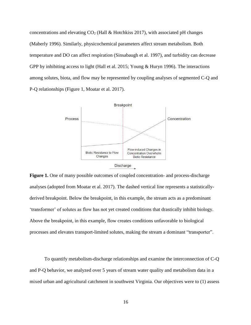
GPP by inhibiting access to light (Hall et al. 2015; Young & Huryn 1996). The interactions

among solutes, biota, and flow may be represented by coupling analyses of segmented C-Q and

P-Q relationships (Figure 1, Moatar et al. 2017).

Figure 1. One of many possible outcomes of coupled concentration- and process-discharge

analyses (adopted from Moatar et al. 2017). The dashed vertical line represents a statistically-

derived breakpoint. Below the breakpoint, in this example, the stream acts as a predominant

‘transformer’ of solutes as flow has not yet created conditions that drastically inhibit biology.

Above the breakpoint, in this example, flow creates conditions unfavorable to biological

processes and elevates transport-limited solutes, making the stream a dominant “transporter”.

To quantify metabolism-discharge relationships and examine the interconnection of C-Q

and P-Q behavior, we analyzed over 5 years of stream water quality and metabolism data in a

mixed urban and agricultural catchment in southwest Virginia. Our objectives were to (1) assess

17

metabolism-Q dynamics to improve our understanding of stream function at different flows and

(2) compare C-Q and metabolism-Q model results to examine the relationship between

biogeochemical processes and physicochemical parameters as they are both acted upon by

changes in flow. We predicted that physicochemical parameters will have opposite, mirrored

trends compared to the processes they affect (e.g., turbidity and GPP) or are affected by (e.g., pH

and ER).

2 Materials and Methods

2.1 Study Site

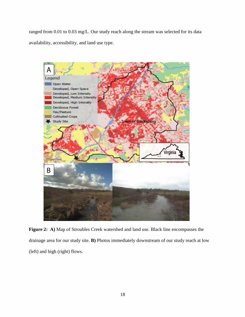
Stroubles Creek (37°12'36'' N, 80°26'42'' W) is a 9.2-mile, third order stream draining a

15 km2 sub-watershed of the New River in Montgomery County of southwest Virginia (Figure

2). Land use in the contributing catchment is approximately 87% developed, 10.9% agriculture,

and 2.9% forest (Homer et al. 2015; Figure 2A), resulting in excess sediment and pathogen

loads. Our study site is a part of the Stream Research, Education, and Management Lab

(StREAM Lab, https://vtstreamlab.weebly.com/). Virginia Tech’s Biological Systems

Engineering Department (BSE) has monitored StREAM Lab since 2008 (Thompson et al. 2012).

In 2010, BSE completed a restoration project that involved removing cattle and sloping back and

stabilizing vertical banks in efforts to remove Stroubles Creek from the EPA’s 303(d) impaired

list for benthic impairment caused by excessive sediment (Wynn et al. 2010). While we do not

have solute data at the same resolution as long-term sensor data, summer sampling in 2018

suggested nitrogen saturation with a low ratio of dissolved organic carbon: nitrate (DOC: NO3),

at ~ 3:1 (O’Donnell, unpublished data). During summer 2018, NO3 ranged from 0.97 to 1.7

mg/L, DOC from 3.0 to 5.6 mg/L, phosphate was consistently below 0.02 mg/L, and ammonium

18

ranged from 0.01 to 0.03 mg/L. Our study reach along the stream was selected for its data

availability, accessibility, and land use type.

Figure 2: A) Map of Stroubles Creek watershed and land use. Black line encompasses the

drainage area for our study site. B) Photos immediately downstream of our study reach at low

(left) and high (right) flows.

19

2.2 Data Collection

High temporal resolution measurements of physicochemical parameters were collected

from 12/10/2012 – 5/1/2018. An in-situ YSI 6920V2 sonde measured conductivity, pH,

dissolved oxygen, turbidity, and temperature at 15-minute intervals. We also recorded dissolved

oxygen data with a PME MiniDOT at 15-minute intervals from 8/31/2017 to 5/1/2018, and these

were used for metabolism measurements from 9/1/2017 – 4/14/18 after a freeze event impaired

dissolved oxygen measurements from the YSI (Figure S1). Sensors were calibrated every 2-4

weeks, and all data were quality-checked to exclude outliers due to sensor error (Text S1, Figure

S2 – S4). A Campbell Scientific CS451 pressure transducer recorded stage at 10-minute

intervals. A stage-discharge relationship developed in 2013 and confirmed using salt dilution

gaging in 2018 was used to calculate discharge using 10-minute stage data. Velocity and width

measurements were taken across multiple years to create relationships with stage. Average

stream channel depth (z) was calculated as , where Q = discharge, v = velocity, and w =

wetted width, to create a stage-depth rating curve. Oxygen at saturation was calculated using

sonde water temperature and barometric pressure (Garcia and Gordon 1992). We obtained light

measurements from a local weather station that uses a Campbell Scientific CS300. We applied

the interp function in R to merge discharge, light, and water quality datasets at matching 30-

minute intervals (R Core Team 2017).

Because daily aggregated medians of physicochemical parameters were needed for the C-

Q analysis, we calculated the daily median of each parameter for days in which sensors collected

measurements for at least 80% of the complete 24-hour period, a percentage we confirmed had

minimal impacts on estimating central tendencies. Daily medians were then natural log-

transformed. pH was not logged because it is log-transformed [H+]. We binned seasons as

20

following: June - August as summer (n=205 total days of data), September - November as fall

(n=180), December - February as winter (n=237), and March - May as spring (n=311).

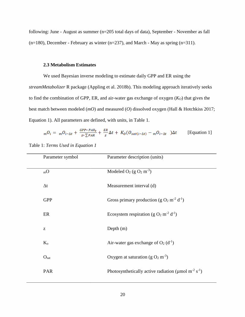
2.3 Metabolism Estimates

We used Bayesian inverse modeling to estimate daily GPP and ER using the

streamMetabolizer R package (Appling et al. 2018b). This modeling approach iteratively seeks

to find the combination of GPP, ER, and air-water gas exchange of oxygen (KO) that gives the

best match between modeled (mO) and measured (O) dissolved oxygen (Hall & Hotchkiss 2017;

Equation 1). All parameters are defined, with units, in Table 1.

[Equation 1]

Table 1: Terms Used in Equation 1

Parameter symbol Parameter description (units)

mO Modeled O2 (g O2 m-3)

Δt Measurement interval (d)

GPP Gross primary production (g O2 m-2 d-1)

ER Ecosystem respiration (g O2 m-2 d-1)

z Depth (m)

Ko Air-water gas exchange of O2 (d-1)

Osat Oxygen at saturation (g O2 m-3)

PAR Photosynthetically active radiation (µmol m-2 s-1)

21

To decrease the likelihood of equifinality of parameter estimates by simultaneously

solving for GPP, ER, and K (Appling et al. 2018a), we took the difference between maximum

and minimum discharge and divided into six bins per year. The hierarchal modeling framework

used by streamMetabolizer then established K~Q relationships by using the bins to constrain air-

water gas exchange (Ko; d-1) as a function of discharge (Appling et al. 2018a). We confirmed

modeled K using nighttime linear regression of dissolved oxygen (Hall & Hotchkiss 2017,

Figure S5). We removed 30 days with K values below the 1% (< 3.38 d-1) and above the 99% (>

27.21 d-1) quantiles to further decrease the chances of using biased metabolism estimates due to

uncertainty in K (Figure S6).

Within streamMetabolizer, we configured specifications for our metabolism estimates

(Supplemental Code S1). We specified a Bayesian model with observation error and process

error. We visualized model convergence of four chains via a traceplot in the rstan package (Stan

Development Team 2018). Based off this traceplot, we used a conservative number of burn-in

steps: 500. Saved steps were set to 2000, and the Markov chain Monte Carlo (mcmc) model

objects were kept on model run to inspect the traceplot. Default package specifications were

otherwise used.

Metabolism estimates passed our model output quality checks for 87% of days with

complete 24-hour datasets (1405/1621 days). However, 216 days of these days were removed

from analysis either due to biologically impossible values (negative GPP or positive ER), poor

model convergence, or poor fit of the modeled O2 data to observed O2. We used diagnostics from

fit() in rstan to quantify model fit, including Rhat and N_eff (Stan Development Team 2018).

Convergence of mcmc occurs when Rhat is equal to 1, so we removed days with Rhat exceeding

1.1 (Gelman and Rubin 1992). N_eff is the number of effective samples, and should be less than

22

the product of the number of mcmc chains run (4) and the number of saved steps (2000) (Howell

2017). Therefore, if the N_eff value ended on or exceeded 8000, we assumed no convergence and

we removed those days. We removed an additional 472 days due to unreasonable K values or

missing physicochemical data. Only days that had solute, discharge, and metabolism estimates

were included in our assessment of site-specific C-Q and metabolism-Q relationships, totaling

933 dates from 2013 - 2018.

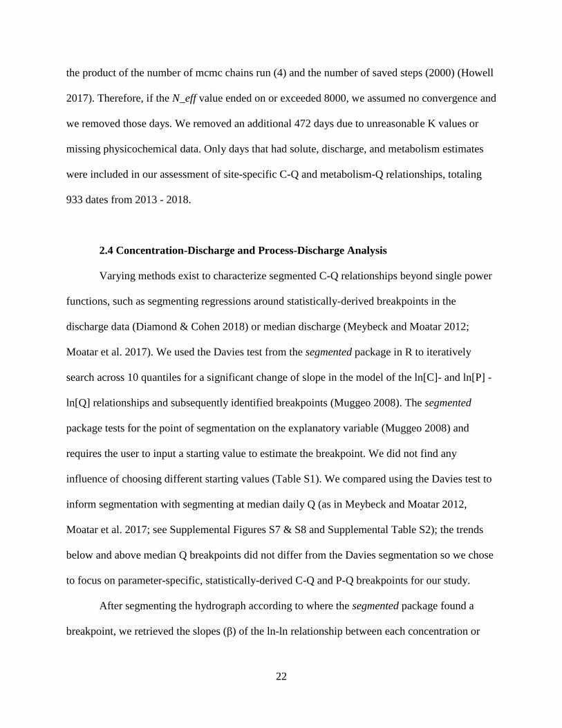
2.4 Concentration-Discharge and Process-Discharge Analysis

Varying methods exist to characterize segmented C-Q relationships beyond single power

functions, such as segmenting regressions around statistically-derived breakpoints in the

discharge data (Diamond & Cohen 2018) or median discharge (Meybeck and Moatar 2012;

Moatar et al. 2017). We used the Davies test from the segmented package in R to iteratively

search across 10 quantiles for a significant change of slope in the model of the ln[C]- and ln[P] -

ln[Q] relationships and subsequently identified breakpoints (Muggeo 2008). The segmented

package tests for the point of segmentation on the explanatory variable (Muggeo 2008) and

requires the user to input a starting value to estimate the breakpoint. We did not find any

influence of choosing different starting values (Table S1). We compared using the Davies test to

inform segmentation with segmenting at median daily Q (as in Meybeck and Moatar 2012,

Moatar et al. 2017; see Supplemental Figures S7 & S8 and Supplemental Table S2); the trends

below and above median Q breakpoints did not differ from the Davies segmentation so we chose

to focus on parameter-specific, statistically-derived C-Q and P-Q breakpoints for our study.

After segmenting the hydrograph according to where the segmented package found a

breakpoint, we retrieved the slopes (β) of the ln-ln relationship between each concentration or

23

metabolism parameter and discharge above and below the breakpoint (Supplemental Code S2).

The slopes can be used to characterize the trends of physicochemical parameters (e.g., Godsey et

al. 2009; Moatar et al. 2017) and metabolism. To test for chemostasis (when β = 0), we used an

analysis of variance test of independence (Ott and Longnecker 2015). We calculated significant

slope differences using a two-tailed z-test (Paternoster et al. 1998). All analyses were conducted

in R (R Core Team 2017).

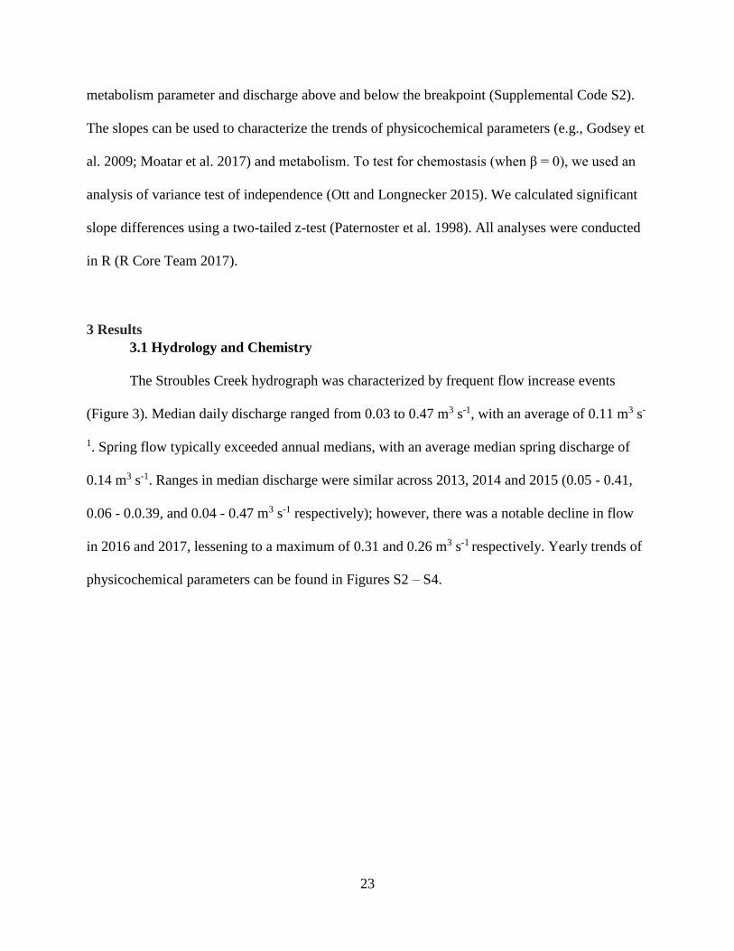
3 Results

3.1 Hydrology and Chemistry

The Stroubles Creek hydrograph was characterized by frequent flow increase events

(Figure 3). Median daily discharge ranged from 0.03 to 0.47 m3 s-1, with an average of 0.11 m3 s-

1. Spring flow typically exceeded annual medians, with an average median spring discharge of

0.14 m3 s-1. Ranges in median discharge were similar across 2013, 2014 and 2015 (0.05 - 0.41,

0.06 - 0.0.39, and 0.04 - 0.47 m3 s-1 respectively); however, there was a notable decline in flow

in 2016 and 2017, lessening to a maximum of 0.31 and 0.26 m3 s-1 respectively. Yearly trends of

physicochemical parameters can be found in Figures S2 – S4.

24

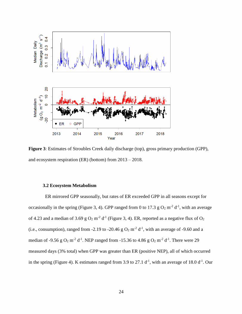
Figure 3: Estimates of Stroubles Creek daily discharge (top), gross primary production (GPP),

and ecosystem respiration (ER) (bottom) from 2013 – 2018.

3.2 Ecosystem Metabolism

ER mirrored GPP seasonally, but rates of ER exceeded GPP in all seasons except for

occasionally in the spring (Figure 3, 4). GPP ranged from 0 to 17.3 g O2 m-2 d-1, with an average

of 4.23 and a median of 3.69 g O2 m-2 d-1 (Figure 3, 4). ER, reported as a negative flux of O2

(i.e., consumption), ranged from -2.19 to -20.46 g O2 m-2 d-1, with an average of -9.60 and a

median of -9.56 g O2 m-2 d-1. NEP ranged from -15.36 to 4.86 g O2 m

-2 d-1. There were 29

measured days (3% total) when GPP was greater than ER (positive NEP), all of which occurred

in the spring (Figure 4). K estimates ranged from 3.9 to 27.1 d-1, with an average of 18.0 d-1. Our

25

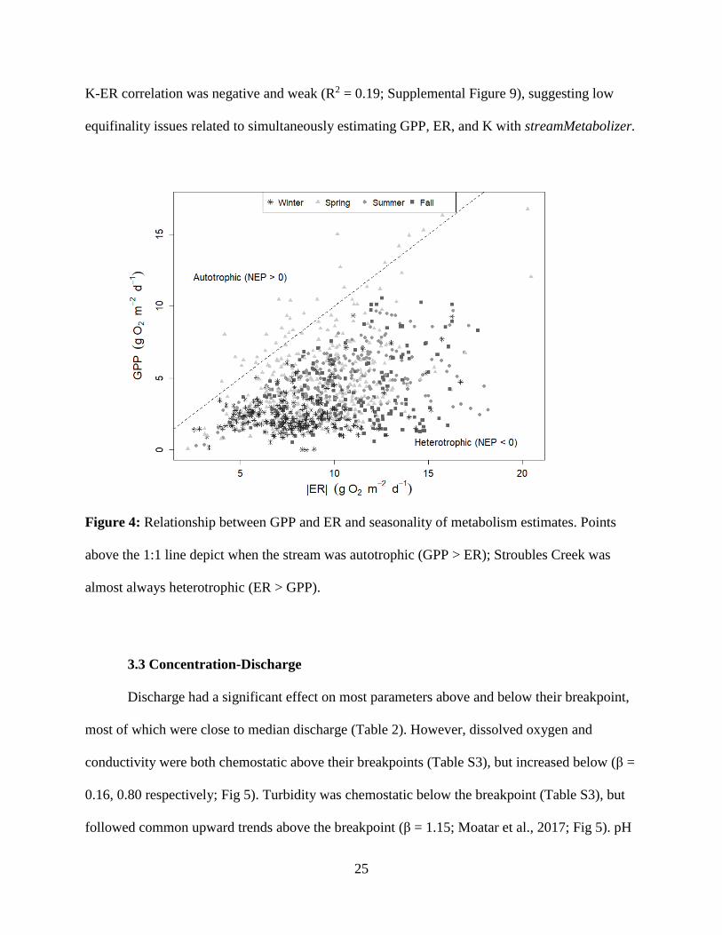
K-ER correlation was negative and weak (R2 = 0.19; Supplemental Figure 9), suggesting low

equifinality issues related to simultaneously estimating GPP, ER, and K with streamMetabolizer.

Figure 4: Relationship between GPP and ER and seasonality of metabolism estimates. Points

above the 1:1 line depict when the stream was autotrophic (GPP > ER); Stroubles Creek was

almost always heterotrophic (ER > GPP).

3.3 Concentration-Discharge

Discharge had a significant effect on most parameters above and below their breakpoint,

most of which were close to median discharge (Table 2). However, dissolved oxygen and

conductivity were both chemostatic above their breakpoints (Table S3), but increased below (β =

0.16, 0.80 respectively; Fig 5). Turbidity was chemostatic below the breakpoint (Table S3), but

followed common upward trends above the breakpoint (β = 1.15; Moatar et al., 2017; Fig 5). pH

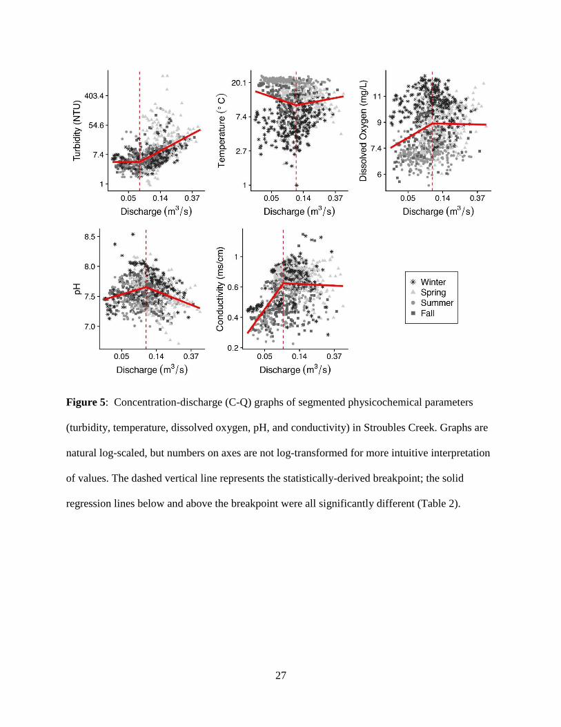
26

declined above the breakpoint (β = -0.23) but increased below (β = 0.17). DO and temperature

varied seasonally, where DO decreased at lower flows below the breakpoint in summer, but

increased during fall and winter (Table S4). Above breakpoints at higher flows, DO declined in

fall and winter but increased in summer. Changes to DO slopes at low and high flows during

spring were not significant. At lower discharges below season-specific breakpoints, temperature

declined in the fall and increased in the winter (Table S4). Above the breakpoint at higher flows,

temperature declined in the winter and increased in fall. Spring and summer temperatures did not

have significant slope breaks above and below breakpoints. When analyzed with all seasons

combined, all physicochemical parameters had significantly different slopes above and below the

breakpoint (Table 2).

27

Figure 5: Concentration-discharge (C-Q) graphs of segmented physicochemical parameters

(turbidity, temperature, dissolved oxygen, pH, and conductivity) in Stroubles Creek. Graphs are

natural log-scaled, but numbers on axes are not log-transformed for more intuitive interpretation

of values. The dashed vertical line represents the statistically-derived breakpoint; the solid

regression lines below and above the breakpoint were all significantly different (Table 2).

28

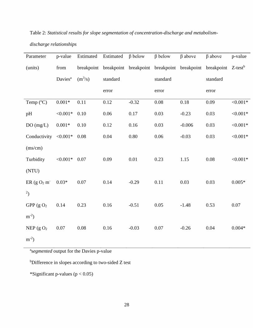
Table 2: Statistical results for slope segmentation of concentration-discharge and metabolism-

discharge relationships

Parameter

(units)

p-value

from

Daviesa

Estimated

breakpoint

(m3/s)

Estimated

breakpoint

standard

error

β below

breakpoint

β below

breakpoint

standard

error

β above

breakpoint

β above

breakpoint

standard

error

p-value

Z-testb

Temp (oC) 0.001* 0.11 0.12 -0.32 0.08 0.18 0.09 <0.001*

pH <0.001* 0.10 0.06 0.17 0.03 -0.23 0.03 <0.001*

DO (mg/L) 0.001* 0.10 0.12 0.16 0.03 -0.006 0.03 <0.001*

Conductivity

(ms/cm)

<0.001* 0.08 0.04 0.80 0.06 -0.03 0.03 <0.001*

Turbidity

(NTU)

<0.001* 0.07 0.09 0.01 0.23 1.15 0.08 <0.001*

ER (g O2 m-

2)

0.03* 0.07 0.14 -0.29 0.11 0.03 0.03 0.005*

GPP (g O2

m-2)

0.14 0.23 0.16 -0.51 0.05 -1.48 0.53 0.07

NEP (g O2

m-2)

0.07 0.08 0.16 -0.03 0.07 -0.26 0.04 0.004*

asegmented output for the Davies p-value

bDifference in slopes according to two-sided Z test

*Significant p-values (p < 0.05)

29

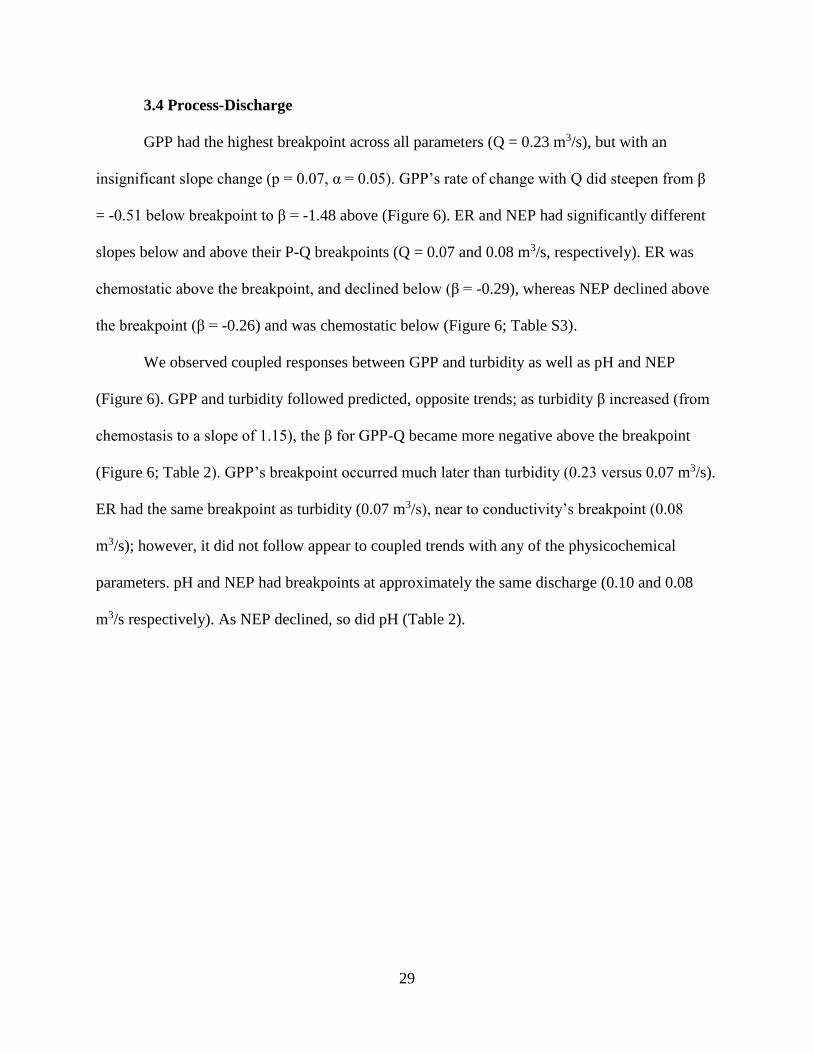
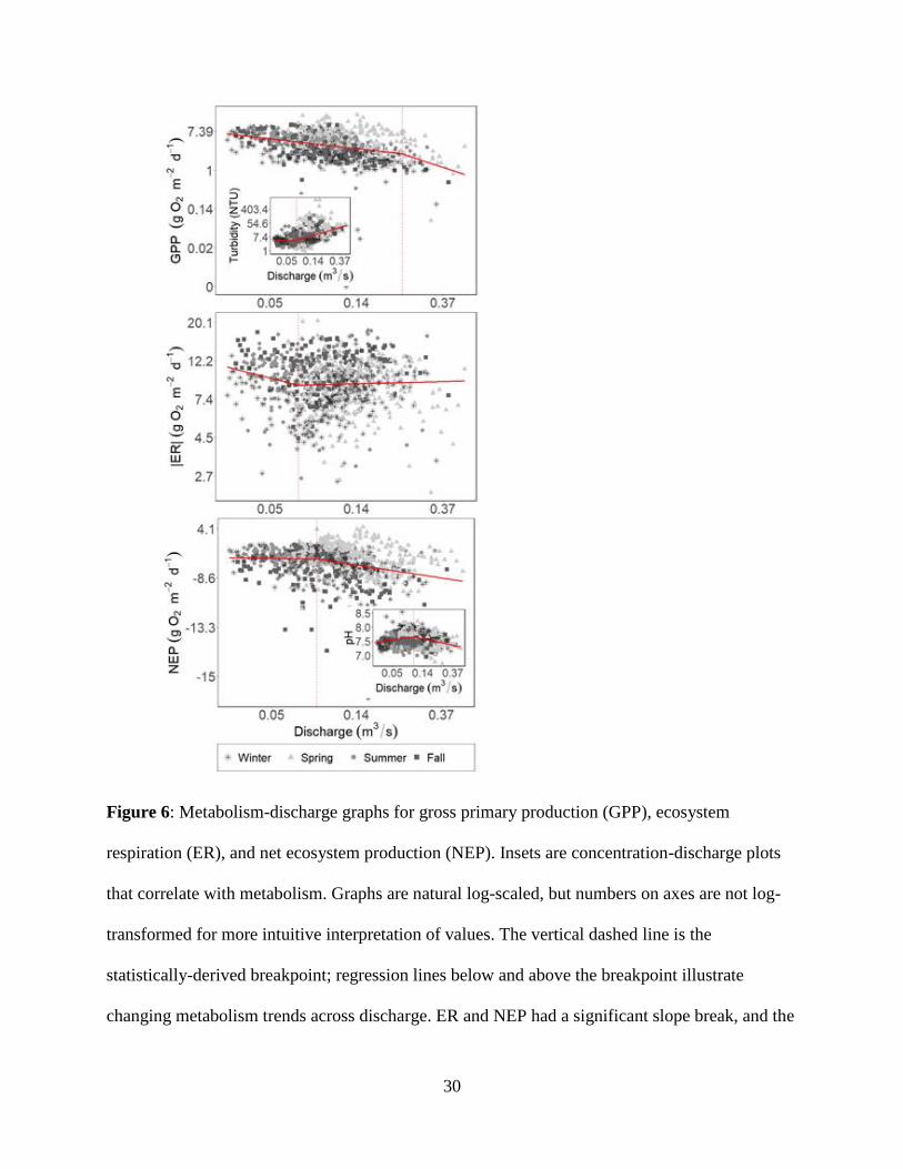
3.4 Process-Discharge

GPP had the highest breakpoint across all parameters (Q = 0.23 m3/s), but with an

insignificant slope change (p = 0.07, α = 0.05). GPP’s rate of change with Q did steepen from β

= -0.51 below breakpoint to β = -1.48 above (Figure 6). ER and NEP had significantly different

slopes below and above their P-Q breakpoints (Q = 0.07 and 0.08 m3/s, respectively). ER was

chemostatic above the breakpoint, and declined below (β = -0.29), whereas NEP declined above

the breakpoint (β = -0.26) and was chemostatic below (Figure 6; Table S3).

We observed coupled responses between GPP and turbidity as well as pH and NEP

(Figure 6). GPP and turbidity followed predicted, opposite trends; as turbidity β increased (from

chemostasis to a slope of 1.15), the β for GPP-Q became more negative above the breakpoint

(Figure 6; Table 2). GPP’s breakpoint occurred much later than turbidity (0.23 versus 0.07 m3/s).

ER had the same breakpoint as turbidity (0.07 m3/s), near to conductivity’s breakpoint (0.08

m3/s); however, it did not follow appear to coupled trends with any of the physicochemical

parameters. pH and NEP had breakpoints at approximately the same discharge (0.10 and 0.08

m3/s respectively). As NEP declined, so did pH (Table 2).

30

Figure 6: Metabolism-discharge graphs for gross primary production (GPP), ecosystem

respiration (ER), and net ecosystem production (NEP). Insets are concentration-discharge plots

that correlate with metabolism. Graphs are natural log-scaled, but numbers on axes are not log-

transformed for more intuitive interpretation of values. The vertical dashed line is the

statistically-derived breakpoint; regression lines below and above the breakpoint illustrate

changing metabolism trends across discharge. ER and NEP had a significant slope break, and the

31

slopes were significantly different. GPP did not have a significant slope break and the slopes

above and below the statistically-derived breakpoint were not significantly different.

4 Discussion

Constant power functions may oversimplify the complex relationship between processes

and discharge. Increasing flow does more than just scour the bed or introduce solutes; it

influences metabolism by changing the physicochemical conditions that underlie microbial

energy production and respiration. We found statistical support for using segmented power law

regressions to quantify distinct changes in ER and NEP with varying discharge above and below

breakpoints. Additionally, C-Q and metabolism-Q relationships of parameters predicted to

directly affect one another - such as turbidity and GPP or pH and NEP – followed coupled

breakpoint behaviors, with varying degrees of statistical significance. These couplings illustrate

the potential utility for using P-Q and C-Q relationships together to explain both functional

responses and biogeochemical consequences of flow changes.

4.1 Concentration-Discharge

Precipitation events are ‘hot moments’ of solute export, shuttling disproportionately large

fluxes of solutes downstream (McClain et al. 2003, Raymond et al. 2016). C-Q relationships are

often used to quantify regimes of solutes at these ‘hot moments’ to better understand downstream

export (Horowitz 2003; Musolff et al. 2015). Transport or source limitations are frequently used

to explain enrichment or dilution trends at higher flows, respectively (Basu et al. 2011, Moatar et

al. 2017). In Stroubles Creek, C-Q trends were similar to findings of other segmented C-Q

studies. Elsewhere, conductivity has predominantly exhibited dilution or chemostasis followed

by dilution (Moatar et al. 2017), though a few other catchments have shown enrichment followed

32

by dilution, similar to our results (Moatar et al. 2017). Although conductivity often exhibits

source-limited dilution across discharge (Diamond and Cohen 2018), the initial increase

observed below the breakpoint may be a result of the dominantly developed catchment that

drains into our study site, as urban streams are inundated with ions that elevate conductivity

(Paul and Meyer 2001, Kaushal et al. 2018). However, higher flows may reverse this trend after

depleting the sources of ions and diluting the concentrations that remain. The enrichment of

turbidity at higher flows at our study site aligned with common dynamics of total suspended

solids across discharge, due to erosion and transport limitation (Moatar et al. 2017). At higher

flows, Stroubles pH exhibited the decline seen in other C-Q studies, potentially as a result of

accessing CO2-rich groundwater or soils (Jenkins 1989, Diamond and Cohen 2018). Dissolved

oxygen and temperature are not typically analyzed in segmented C-Q studies focused on

describing solute transport. The C-Q relationships for dissolved oxygen and temperature are

heavily influenced by seasonality (Figure 5; Table S4). Overall, the similarity of Stroubles Creek

physicochemical trends to those seen in other streams makes the findings of our coupled C-Q

and P-Q relationships applicable to other systems. However, classifying C-Q dynamics by

transport or source limitations alone may not capture physicochemical behavior across discharge.

4.2 Process-Discharge

Precipitation events generate multiple abiotic changes that can influence stream

ecosystem processes: flow increases, physicochemical conditions are altered, and cloud cover

reduces photosynthetically active radiation. Yet, we do not account for likely thresholds or

breakpoints in processes the same way we do for physicochemical-discharge relationships.

Ultimately, statistically-derived segmented P-Q relationships allow us to quantify when a stream

33

becomes a predominant ‘transporter’ from ‘transformer’ by determining if and when a significant

threshold of process resistance to discharge exists.

Within a stream at a precipitation event scale, GPP is negatively impacted by flow

(Fisher 1982, Reisinger et al. 2017). GPP also declined at our study site, appearing to have a

greater reduction with flow above a breakpoint threshold (Figure 6), potentially as a result of

enhanced scouring or cloud cover. GPP trends above and below the breakpoint were not

significantly different however (Table 2). Consequently, we did not detect a significantly greater

GPP reduction at higher flows as a result of the compounding influence of elevated turbidity,

reduced light, or intensified scour. While our data suggest a higher threshold and later breakpoint

(0.23 m3/s) for GPP relative to any other metabolism or concentration-discharge relationships

(Fig 6), this higher breakpoint means we did not have enough estimates of GPP from enough

high-flow events to find a statistically significant change in slope (Table 2). Moreover,

seasonality may significantly influence segmented P-Q patterns. To examine the impact of

seasonality and yearly data on metabolism-Q relationships, we conducted breakpoint analyses

per scenario (each season, each year). Although we did not have enough data to detect significant

differences for most metabolism-Q relationships when data were subset, GPP was consistently,

significantly negative above the breakpoint for four scenarios (i.e., 2018, 2013, fall, spring), out

of ten total scenarios (Figure S10). The presence of a significant slope change for these

scenarios, but not for the composite P-Q for all GPP estimates, may indicate that variability from

the insignificant scenarios may drive the lack of a significant slope change for all estimates.

ER is also affected by flow-induced changes: reductions in residence time, scour that

may remove respiring microbes, and influxes of terrestrial organic matter. Storms frequently

increase ER (Roley et al. 2014), potentially as a result of the increased concentrations of

34

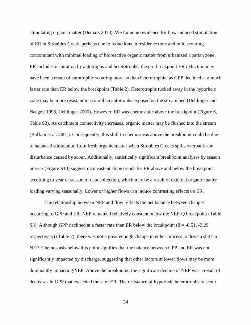
stimulating organic matter (Demars 2018). We found no evidence for flow-induced stimulation

of ER in Stroubles Creek, perhaps due to reductions in residence time and mild scouring

concomitant with minimal loading of bioreactive organic matter from urbanized riparian zone.

ER includes respiration by autotrophs and heterotrophs; the pre-breakpoint ER reduction may

have been a result of autotrophic scouring more so than heterotrophic, as GPP declined at a much

faster rate than ER below the breakpoint (Table 2). Heterotrophs tucked away in the hyporheic

zone may be more resistant to scour than autotrophs exposed on the stream bed (Uehlinger and

Naegeli 1998, Uehlinger 2000). However, ER was chemostatic above the breakpoint (Figure 6,

Table S3). As catchment connectivity increases, organic matter may be flushed into the stream

(Buffam et al. 2001). Consequently, this shift to chemostasis above the breakpoint could be due

to balanced stimulation from fresh organic matter when Stroubles Creeks spills overbank and

disturbance caused by scour. Additionally, statistically significant breakpoint analyses by season

or year (Figure S10) suggest inconsistent slope trends for ER above and below the breakpoint

according to year or season of data collection, which may be a result of external organic matter

loading varying seasonally. Lower or higher flows can induce contrasting effects on ER.

The relationship between NEP and flow reflects the net balance between changes

occurring to GPP and ER. NEP remained relatively constant below the NEP-Q breakpoint (Table

S3). Although GPP declined at a faster rate than ER below the breakpoint (β = -0.51, -0.29

respectively) (Table 2), there was not a great enough change in either process to drive a shift in

NEP. Chemostasis below this point signifies that the balance between GPP and ER was not

significantly impacted by discharge, suggesting that other factors at lower flows may be more

dominantly impacting NEP. Above the breakpoint, the significant decline of NEP was a result of

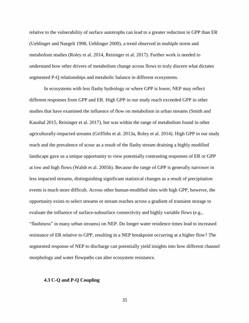
decreases in GPP that exceeded those of ER. The resistance of hyporheic heterotrophs to scour

35

relative to the vulnerability of surface autotrophs can lead to a greater reduction in GPP than ER

(Uehlinger and Naegeli 1998, Uehlinger 2000), a trend observed in multiple storm and

metabolism studies (Roley et al. 2014, Reisinger et al. 2017). Further work is needed to

understand how other drivers of metabolism change across flows to truly discern what dictates

segmented P-Q relationships and metabolic balance in different ecosystems.

In ecosystems with less flashy hydrology or where GPP is lower, NEP may reflect

different responses from GPP and ER. High GPP in our study reach exceeded GPP in other

studies that have examined the influence of flow on metabolism in urban streams (Smith and

Kaushal 2015, Reisinger et al. 2017), but was within the range of metabolism found in other

agriculturally-impacted streams (Griffiths et al. 2013a, Roley et al. 2014). High GPP in our study

reach and the prevalence of scour as a result of the flashy stream draining a highly modified

landscape gave us a unique opportunity to view potentially contrasting responses of ER or GPP

at low and high flows (Walsh et al. 2005b). Because the range of GPP is generally narrower in

less impacted streams, distinguishing significant statistical changes as a result of precipitation

events is much more difficult. Across other human-modified sites with high GPP, however, the

opportunity exists to select streams or stream reaches across a gradient of transient storage to

evaluate the influence of surface-subsurface connectivity and highly variable flows (e.g.,

“flashiness” in many urban streams) on NEP. Do longer water residence times lead to increased

resistance of ER relative to GPP, resulting in a NEP breakpoint occurring at a higher flow? The

segmented response of NEP to discharge can potentially yield insights into how different channel

morphology and water flowpaths can alter ecosystem resistance.

4.3 C-Q and P-Q Coupling

36

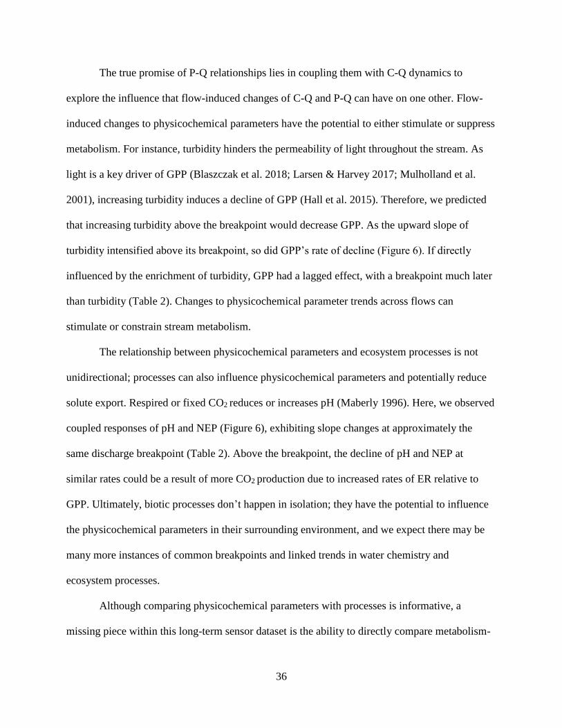
The true promise of P-Q relationships lies in coupling them with C-Q dynamics to

explore the influence that flow-induced changes of C-Q and P-Q can have on one other. Flow-

induced changes to physicochemical parameters have the potential to either stimulate or suppress

metabolism. For instance, turbidity hinders the permeability of light throughout the stream. As

light is a key driver of GPP (Blaszczak et al. 2018; Larsen & Harvey 2017; Mulholland et al.

2001), increasing turbidity induces a decline of GPP (Hall et al. 2015). Therefore, we predicted

that increasing turbidity above the breakpoint would decrease GPP. As the upward slope of

turbidity intensified above its breakpoint, so did GPP’s rate of decline (Figure 6). If directly

influenced by the enrichment of turbidity, GPP had a lagged effect, with a breakpoint much later

than turbidity (Table 2). Changes to physicochemical parameter trends across flows can

stimulate or constrain stream metabolism.

The relationship between physicochemical parameters and ecosystem processes is not

unidirectional; processes can also influence physicochemical parameters and potentially reduce

solute export. Respired or fixed CO2 reduces or increases pH (Maberly 1996). Here, we observed

coupled responses of pH and NEP (Figure 6), exhibiting slope changes at approximately the

same discharge breakpoint (Table 2). Above the breakpoint, the decline of pH and NEP at

similar rates could be a result of more CO2 production due to increased rates of ER relative to

GPP. Ultimately, biotic processes don’t happen in isolation; they have the potential to influence

the physicochemical parameters in their surrounding environment, and we expect there may be

many more instances of common breakpoints and linked trends in water chemistry and

ecosystem processes.

Although comparing physicochemical parameters with processes is informative, a

missing piece within this long-term sensor dataset is the ability to directly compare metabolism-

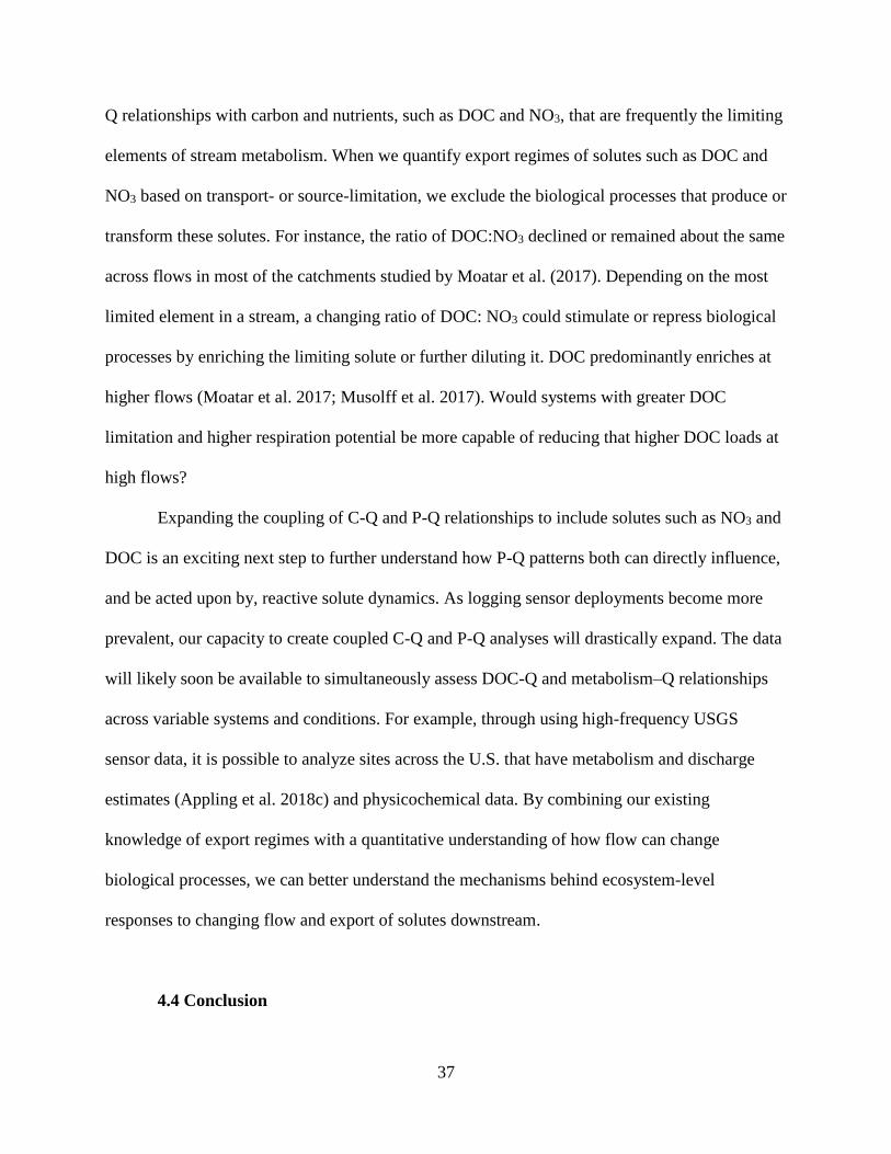
37

Q relationships with carbon and nutrients, such as DOC and NO3, that are frequently the limiting

elements of stream metabolism. When we quantify export regimes of solutes such as DOC and

NO3 based on transport- or source-limitation, we exclude the biological processes that produce or

transform these solutes. For instance, the ratio of DOC:NO3 declined or remained about the same

across flows in most of the catchments studied by Moatar et al. (2017). Depending on the most

limited element in a stream, a changing ratio of DOC: NO3 could stimulate or repress biological

processes by enriching the limiting solute or further diluting it. DOC predominantly enriches at

higher flows (Moatar et al. 2017; Musolff et al. 2017). Would systems with greater DOC

limitation and higher respiration potential be more capable of reducing that higher DOC loads at

high flows?

Expanding the coupling of C-Q and P-Q relationships to include solutes such as NO3 and

DOC is an exciting next step to further understand how P-Q patterns both can directly influence,

and be acted upon by, reactive solute dynamics. As logging sensor deployments become more

prevalent, our capacity to create coupled C-Q and P-Q analyses will drastically expand. The data

will likely soon be available to simultaneously assess DOC-Q and metabolism–Q relationships

across variable systems and conditions. For example, through using high-frequency USGS

sensor data, it is possible to analyze sites across the U.S. that have metabolism and discharge

estimates (Appling et al. 2018c) and physicochemical data. By combining our existing

knowledge of export regimes with a quantitative understanding of how flow can change

biological processes, we can better understand the mechanisms behind ecosystem-level

responses to changing flow and export of solutes downstream.

4.4 Conclusion

38

Stream flow changes have hydrologic and biogeochemical consequences. Hydrologically,

higher flows are regarded as agents of catchment connectivity, simultaneously unleashing or

diluting solutes into freshwater ecosystems. Biogeochemically, physical disturbances caused by

higher flows disrupt ecosystem processes by moving the stream bed or reducing transient

storage. However, insight into the mechanisms behind C-Q and P-Q dynamics across flow is

limited when we view one without the other; physicochemical parameters influence, and are

influenced by, in-stream biology. To understand ecosystem responses at different flows, we must

integrate the interactions between flow, ecosystem process, and C-Q dynamics into our analyses

of stream function. By coupling C-Q and P-Q relationships, we can better understand how

ecosystems respond to, influence, and recover from the many physical and chemical changes that

occur with altered flow.

Acknowledgements

Data used in our analysis can be found in the Supplemental Information in Dataset 1. Data were

made available by sensors employed by Virginia Tech’s StREAM Lab, funded by the VT-BSE

for baseline StREAM Lab maintenance and monitoring. Site flow photos were provided by

Virginia Tech’s StREAM Lab camera. We thank D. McLaughlin for his thoughtful edits, W.C.

Hession for sharing these data and his knowledge of Stroubles Creek, and L. Lehmann for

assisting with database access and questions.

39

References

APPLING, A., R. HALL, M. ARROITA, AND C. B. YACKULIC. 2018a. streamMetabolizer:

Models for Estimating Aquatic Photosynthesis and Respiration.

APPLING, A. P., R. O. HALL, C. B. YACKULIC, AND M. ARROITA. 2018b. Overcoming

Equifinality: Leveraging Long Time Series for Stream Metabolism Estimation. Journal of

Geophysical Research: Biogeosciences.

APPLING, A., J. S. READ, L. A. WINSLOW, M. ARROITA, E. S. BERNHARDT, N. A.

GRIFFITHS, R. O. HALL, J. W. HARVEY, J. B. HEFFERNAN, E. H. STANLEY, E. G.

STETS, AND C. B. YACKULIC. 2018c. The metabolic regimes of 356 rivers in the United

States Background &amp; Summary. Sci. Data 5.

BASU, N. B., S. E. THOMPSON, AND P. S. C. RAO. 2011. Hydrologic and biogeochemical

functioning of intensively managed catchments: A synthesis of top-down analyses. Water

Resources Research 47.

BLASZCZAK, J. R., J. M. DELESANTRO, D. L. URBAN, M. W. DOYLE, AND E. S.

BERNHARDT. 2018. Scoured or suffocated: Urban stream ecosystems oscillate between

hydrologic and dissolved oxygen extremes. Limnology and Oceanography 00:1–18.

BOYER, E. W., G. M. HORNBERGER, K. E. BENCALA, AND D. M. MCKNIGHT. 1997.

Response characteristics of DOC flushing in an alpine catchment. Hydrological Processes

11:1635–1647.

BUFFAM, I., J. GALLOWAY, L. BLUM, AND K. MCGLATHERY. 2001. A

stormflow/baseflow comparison of dissolved organic matter concentrations and bioavailability in

an Appalachian stream. Biogeochemistry 53:269–306.

COLE, J. J., Y. T. PRAIRIE, N. F. CARACO, W. H. MCDOWELL, L. J. TRANVIK, R. G.

STRIEGL, C. M. DUARTE, P. KORTELAINEN, J. A. DOWNING, J. J. MIDDELBURG, AND

J. MELACK. 2007. Plumbing the Global Carbon Cycle: Integrating Inland Waters into the

Terrestrial Carbon Budget. Ecosystems 10:172–185.

DEMARS, B. O. L. 2018. Hydrological pulses and burning of dissolved organic carbon by

stream respiration. Limnology and Oceanography.

DIAMOND, J. S., AND M. J. COHEN. 2018. Complex patterns of catchment solute-discharge

relationships for coastal plain rivers. Hydrological Processes 32:388–401.

DODDS, W. K., E. MARTÍ, J. L. TANK, J. PONTIUS, S. K. HAMILTON, N. B. GRIMM, W.

B. BOWDEN, W. H. MCDOWELL, B. J. PETERSON, H. M. VALETT, J. R. WEBSTER, AND

S. GREGORY. 2004. Carbon and nitrogen stoichiometry and nitrogen cycling rates in streams.

Oecologia 140:458–467.

DRUMMOND, J., S. BERNAL, D. VON SCHILLER, AND E. MARTÍ. 2016. Freshwater

Science. Freshwater Science 35:1176–1188.

FISHER, S. G. 1982. Temporal succession in a desert stream ecosystem following flash

flooding. Ecological Monographs 52:93–110.

40

FISHER, S. G., N. B. GRIMM, N. MARTÍ, R. M. HOLMES, AND J. B. JONES. 1998. Material

Spiraling in Stream Corridors: A Telescoping Ecosystem Model. Ecosystems 1:19–34.

GARCIA, H. E., AND L. I. GORDON. 1992. Oxygen solubility in seawater: Better fitting

equations. Limnology and Oceanography 37:1307–1312.

GASITH, A., AND V. H. RESH. 1999. Streams in Mediterranean Climate Regions: Abiotic

Influences and Biotic Responses to Predictable Seasonal Events. Annual Review of Ecology and

Systematics 30:51–81.

GELMAN, A., AND D. B. RUBIN. 1992. Inference from Iterative Simulation Using Multiple

Sequences. Statistical Science 7:457–472.

GODSEY, S. E., J. W. KIRCHNER, AND D. W. CLOW. 2009. Concentration-discharge

relationships reflect chemostatic characteristics of US catchments. Hydrological Processes

23:1844–1864.

GRIFFITHS, N. A., J. L. TANK, T. V. ROYER, S. S. ROLEY, E. J. ROSI-MARSHALL, M. R.

WHILES, J. J. BEAULIEU, AND L. T. JOHNSON. 2013. Agricultural land use alters the

seasonality and magnitude of stream metabolism. Limnology and Oceanography 58:1513–1529.

HALL, R., M. BAKER, C. D. ARP, AND B. J. KOCH. 2009. Robert O. Hall, Jr., Michelle A.

Baker, Christopher D. Arp, and Benjamin J. Koch. Hydrologic control of nitrogen removal,

storage, and export in a mountain stream. Limnol. Oceanogr., 54(6), 2009, 2128–2142. Limnol.

Oceanogr. 43:2128–2142.

HALL, R., AND E. HOTCHKISS. 2017. Stream Metabolism. Pages 219–235 in G. Lamberti

and R. Hauer (editors). Methods in Stream Ecology, Vol 2: Ecosystem FunctionThird Edit.

Elsevier.

HALL, R., C. B. YACKULIC, T. A. KENNEDY, M. D. YARD, E. J. ROSI-MARSHALL, N.

VOICHICK, AND K. E. BEHN. 2015. Turbidity, light, temperature, and hydropeaking control

primary productivity in the Colorado River, Grand Canyon. Limnology and Oceanography

60:512–526.

HERNDON, E. M., A. L. DERE, P. L. SULLIVAN, D. B. NORRIS REYNOLDS, A. E. M

HERNDON, D. NORRIS, B. REYNOLDS, S. L. BRANTLEY, AND A. L. DERE. 2015.

Landscape heterogeneity drives contrasting concentration–discharge relationships in shale

headwater catchments. Hydrol. Earth Syst. Sci 19:3333–3347.

HOMER, C. G., J. DEWITZ, L. YANG, S. JIN, P. DANIELSON, XIAN, J. COULSTON, N.

HEROLD, J. WICKHAM, AND K. MEGOWN. 2015. Completion of the 2011 National Land

Cover Database for the conterminous United States – representing a decade of land cover change

information. Photogrammetric Engineering and Remote Sensing 81:345–353.

HOROWITZ, A. J. 2003. An evaluation of sediment rating curves for estimating suspended

sediment concentrations for subsequent flux calculations. Hydrological Processes 17:3387–3409.

HOWELL, J. 2017. Stan Best Practices. https://github.com/stan-dev/stan/wiki/Stan-Best-

Practices.

41

INAMDAR, S. P., S. F. CHRISTOPHER, AND M. J. MITCHELL. 2004. Export mechanisms

for dissolved organic carbon and nitrate during summer storm events in a glaciated forested

catchment in New York, USA. Process 18:2651–2661.

JENKINS, A. 1989. Storm period hydrochemical response in an unforested Scottish catchment.

Hydrological Sciences Journal 34:393–404.

KAUSHAL, S. S., G. E. LIKENS, M. L. PACE, R. M. UTZ, S. HAQ, J. GORMAN, AND M.

GRESE. 2018. Freshwater salinization syndrome on a continental scale. Proceedings of the

National Academy of Sciences of the United States of America 115:E574–E583.

LAMBERTI, G. A., AND A. D. STEINMAN. 1997. A Comparison of Primary Production in

Stream Ecosystems. Journal of the North American Benthological Society 16:95–104.

LARSEN, L. G., AND J. W. HARVEY. 2017. Disrupted carbon cycling in restored and

unrestored urban streams: Critical timescales and controls. Limnology and Oceanography

62:S160–S182.

MABERLY, S. C. 1996. Diel, episodic and seasonal changes in pH and concentrations of

inorganic carbon in a productive lake. Freshwater Biology 35:579–598.

MCCLAIN, M. E., E. W. BOYER, C. L. DENT, S. E. GERGEL, N. B. GRIMM, P. M.

GROFFMAN, S. C. HART, J. W. HARVEY, C. A. JOHNSTON, E. MAYORGA, W. H.

MCDOWELL, AND G. PINAY. 2003. Biogeochemical Hot Spots and Hot Moments at the

Interface of Terrestrial and Aquatic Ecosystems. Ecosystems 6:301–312.

MCGLYNN, B. L., AND J. J. MCDONNELL. 2003. Quantifying the relative contributions of

riparian and hillslope zones to catchment runoff. Water Resources Research 39.

MCLAUGHLIN, C., AND L. A. KAPLAN. 2013. Biological lability of dissolved organic

carbon in stream water and contributing terrestrial sources. Freshwater Science 32:1219–1230.

MCMILLAN, S. K., H. F. WILSON, C. L. TAGUE, D. M. HANES, S. INAMDAR, D. L.

KARWAN, T. LOECKE, J. MORRISON, S. F. MURPHY, AND P. VIDON. 2018. Before the

storm: antecedent conditions as regulators of hydrologic and biogeochemical response to

extreme climate events. Biogeochemistry:1–15.

MEYBECK, M., AND F. MOATAR. 2012. Daily variability of river concentrations and fluxes:

indicators based on the segmentation of the rating curve. Hydrological Processes 26:1188–1207.

MOATAR, F., B. W. ABBOTT, C. MINAUDO, F. CURIE, AND G. PINAY. 2017. Elemental

properties, hydrology, and biology interact to shape concentration-discharge curves for carbon,

nutrients, sediment, and major ions. Water Resources Research 53:1270–1287.

MUGGEO, V. M. R. 2008. segmented: an R Package to Fit Regression Models with Broken-

Line Relationships.

MULHOLLAND, P. J. 1992. Regulation of nutrient concentrations in a temperate forest stream:

Roles of upland, riparian, and instream processes. Limnology and Oceanography 37:1512–1526.

MULHOLLAND, P. J., C. S. FELLOWS, J. L. TANK, N. B. GRIMM, J. R. WEBSTER, S. K.

HAMILTON, E. MARTI, L. ASHKENAS, W. B. BOWDEN, W. K. DODDS, W. H.

42

MCDOWELL, M. J. PAUL, AND B. J. PETERSON. 2001. Inter-biome comparison of factors

controlling stream metabolism. Freshwater Biology 46:1503–1517.

MULHOLLAND, P. J., AND W. R. HILL. 1997. Seasonal patterns in streamwater nutrient and

dissolved organic carbon concentrations: Separating catchment flow path and in-stream effects.

WATER RESOURCES RESEARCH 33:1297–1306.

MUSOLFF, A., J. H. FLECKENSTEIN, P. S. C. RAO, AND J. W. JAWITZ. 2017. Emergent

archetype patterns of coupled hydrologic and biogeochemical responses in catchments.

Geophysical Research Letters 44:4143–4151.

MUSOLFF, A., C. SCHMIDT, B. SELLE, AND J. H. FLECKENSTEIN. 2015. Catchment

controls on solute export. Advances in Water Resources 86:133–146.

ODUM, E. P., J. T. FINN, AND E. H. FRANZ. 1979. Perturbation Theory and the Subsidy-

Stress Gradient. BioScience 29:349–352.

OTT, R. L., AND M. T. LONGNECKER. 2015. An introduction to statistical methods and data

analysis. Nelson Education.

PATERNOSTER, R., R. BRAME, P. MAZEROLE, AND A. PIQUERO. 1998. Using the

correct statistical test for the equality of regression coefficients. Criminology 36:859–866.

PAUL, M. J., AND J. L. MEYER. 2001. Streams in the Urban Landscape. Annual Review of

Ecology and Systematics 32:333–365.

POFF, N. L., J. D. ALLAN, M. B. BAIN, J. R. KARR, K. L. PRESTEGAARD, B. D.

RICHTER, R. E. SPARKS, AND J. C. STROMBERG. 1997. The Natural Flow Regime.

BioScience 47:769–784.

RAYMOND, P. A., J. E. SAIERS, AND W. V. SOBCZAK. 2016. Hydrological and

biogeochemical controls on watershed dissolved organic matter transport: Pulse- shunt concept.

Ecology 97.

REISINGER, A. J., E. J. ROSI, H. A. BECHTOLD, T. R. DOODY, S. S. KAUSHAL, AND P.

M. GROFFMAN. 2017. Recovery and resilience of urban stream metabolism following

Superstorm Sandy and other floods. Ecosphere 8.

ROBERTS, B. J., AND P. J. MULHOLLAND. 2007. In-stream biotic control on nutrient

biogeochemistry in a forested stream, West Fork of Walker Branch. Journal of Geophysical

Research: Biogeosciences 112:n/a-n/a.

ROLEY, S. S., J. L. TANK, N. A. GRIFFITHS, R. O. HALL, AND R. T. DAVIS. 2014. The

influence of floodplain restoration on whole-stream metabolism in an agricultural stream:

insights from a 5-year continuous data set. Freshwater Science 33:1043–1059.

SEYBOLD, E., AND B. MCGLYNN. 2018. Hydrologic and biogeochemical drivers of

dissolved organic carbon and nitrate uptake in a headwater stream network. Biogeochemistry

138:23–48.

SINSABAUGH, R. L., G. W. MINSHALL, R. C. PETERSEN, K. W. CUMMINS, T. L. BOTT,

J. R. SEDELL, C. E. CUSHING, P. J. MULHOLLAND, J. D. NEWBOLD, AND J. W.

43

ELWOOD. 1997. Large-Scale Trends for Stream Benthic Respiration. Source Journal of the

North American Benthological Society 16:119–122.

SMITH, R. M., AND S. S. KAUSHAL. 2015. Carbon cycle of an urban watershed: exports,

sources, and metabolism. Biogeochemistry 126:173–195.

STAN DEVELOPMENT TEAM. 2018. {RStan}: the {R} interface to {Stan}.

THOMPSON, W., C. HESSION, AND D. SCOTT. 2012. StREAM Lab at Virginia Tech.

Resources Mag. 19:8–9.

UEHLINGER, U. 2000. Resistance and resilience of ecosystem metabolism in a flood-prone

river system. Freshwater Biology 45:319–332.

UEHLINGER, U., AND M. W. NAEGELI. 1998. Ecosystem Metabolism, Disturbance, and

Stability in a Prealpine Gravel Bed River. Journal of the North American Benthological Society

17:165–178.

WALSH, C., A. ROY, J. FEMINELLA, P. COTTINGHAM, P. GROFFMAN, AND R.

MORGAN. 2005. The urban stream syndrome: current knowledge and the search for a cure. J N

Am. Benthol. Soc.

WILLIAMS, G. P. 1989. Sediment concentration versus water discharge during single

hydrologic events in rivers. Journal of Hydrology 111:89–106.

WOLLHEIM, W. M., S. BERNAL, D. A. BURNS, J. A. CZUBA, C. T. DRISCOLL, A. T.

HANSEN, R. T. HENSLEY, J. D. HOSEN, S. INAMDAR, S. S. KAUSHAL, L. E. KOENIG,

Y. H. LU, A. MARZADRI, P. A. RAYMOND, D. SCOTT, R. J. STEWART, P. G. VIDON,

AND E. WOHL. 2018. River network saturation concept: factors influencing the balance of

biogeochemical supply and demand of river networks. Biogeochemistry:1–19.

WYNN, T., C. HESSION, AND G. YAGOW. 2010. Stroubles Creek Stream Restoration.

Richmond.

YOUNG, R. G., AND A. D. HURYN. 1996. Interannual variation in discharge controls

ecosystem metabolism along a grassland river continuum. Canadian Journal of Fisheries and

Aquatic Sciences 53:2199–2211.

ZHANG, Q., C. J. HARMAN, AND W. P. BALL. 2016. An improved method for interpretation

of riverine concentration-discharge relationships indicates long-term shifts in reservoir sediment

trapping. Geophysical Research Letters 43:10,215-10,224.

44

Chapter Three: Resistance and resilience of stream metabolism to high flow disturbances

B. O’Donnell1*, E. R. Hotchkiss1

1Department of Biological Sciences, Virginia Tech

*Corresponding author: Brynn O’Donnell (brynnmodonnell@gmail.com)

Target Journal Submission: Biogeosciences

Abstract. Streams are ecosystems organized by disturbance, and one of the most frequent

disturbances to a stream is elevated flow. Yet, our knowledge of how stream processes, such as

stream metabolism, respond to higher flow events is limited. Stream metabolism is the fixation

(gross primary production; GPP) and respiration (ecosystem respiration; ER) of carbon within an

ecosystem. We still lack a general predictive framework for understanding controls on within-

site variation of metabolic responses to flow disturbances. Using five years of high-frequency

dissolved oxygen data from an urban- and agriculturally-influenced stream, we estimated GPP

and ER across 15 isolated high flow events. Metabolism is dynamic from day to day, even at low

flows. Thus, we quantified metabolic resistance as the magnitude of departure from the

antecedent, dynamic equilibrium at lower flows, and calculated resilience as the days until

metabolism returned to dynamic equilibrium. We evaluated how characteristics of each high

flow event (such as size), antecedent conditions, and time since last flow disturbance correlated

with metabolic resistance and resilience. ER was both more resistant and resilient than GPP. GPP

was typically suppressed following flow disturbances, regardless of flow disturbance intensity.

However, ER magnitude of departure increased with intensity of flow disturbance. Additionally,

GPP was less resilient and took longer to recover (0 to >9 days, mean = 2.2) than ER (0 to 2

days, mean = 0.6). Because of the projected increase in storms, the flashy nature of altered

streams, and the substantial effect of flow on ecosystem function, it is essential that we

45

understand how GPP and ER respond to flow disturbances of various magnitudes and across

multiple seasons and environmental conditions.

1 Introduction

Disturbance is a key driver of stream ecosystem function, influencing everything from

carbon and nutrient export to energy flow (Stanley et al. 2010). Stream biogeochemical

processes can be altered via long-term, ‘press’ disturbances, such as land use change (Plont et al.,

in review), or by episodic ‘pulse’ disturbances, such as transitory changes in allochthonous

inputs (Bender et al. 1984, Dodds et al. 2004, Seybold and McGlynn 2018). Disturbance creates

patterns in stream processes (Resh et al. 1988, Stanley et al. 2010), generating oscillations that

form a pulsing steady state (sensu Odum et al. 1995). Here, we use the definition of disturbance

from White and Pickett (1985): “any relatively discrete event in time that disrupts the

ecosystem… and changes resources, substrate availability, or the physical environment”.

Disturbances to streams come in many forms, including: spates or rapid increases in the volume

of water, drought, substratum movement, and anthropogenic alterations of channel morphology,

flow, or solute chemistry (Resh et al. 1988).

Elevated flow is one of the most pervasive, frequent disturbances to streams. Flow

disturbances can scour the benthos, increase turbidity, and reduce light – all of which can

negatively impact stream function (Hall et al. 2015, Blaszczak et al. 2018). However, flow is an

inherent characteristic of streams and may influence stream function along a “subsidy-stress”

gradient (sensu Odum et al. 1979). Excessively high flows can stress stream biota and induce

conditions unfavorable for biotic processes, whereas ‘normal’ flows can stimulate internal

biogeochemical transformations by flushing in subsidizing inputs of limiting nutrients or organic

matter (Lamberti and Steinman 1997). Whether flow subsidizes or stresses the stream can

46

depend on a variety of factors, including the ecosystem process of interest, but ultimately flow is

a disturbance when it exceeds some certain threshold.

Stream metabolism is an integrative whole-ecosystem estimate of the carbon fixed and

broken down by autotrophs and heterotrophs within a stream, and is most commonly estimated

via diel changes in dissolved oxygen (Hall and Hotchkiss 2017). Autotrophs produce oxygen via

gross primary production (GPP), and both auto- and heterotrophs consume oxygen during

ecosystem respiration (ER). Together, ER and GPP are opposing processes with respect to

carbon balance and sum to net ecosystem production (NEP), which can elucidate whether a

stream is a net producer (autotrophic; GPP > ER) or consumer (heterotrophic; ER > GPP) of

carbon. Ecosystem metabolism is increasingly used to understand the health of streams (Young

et al. 2008) and ecosystem responses to disturbance (e.g., Arroita et al. 2019), and is tightly

coupled with other ecosystem processes (e.g., nitrogen uptake, Hall and Tank 2003).

Metabolism is influenced by many abiotic and biotic factors. GPP increases with light

(Mulholland et al. 2001, Roberts and Mulholland 2007), nutrient availability (Grimm and Fisher

1986, Mulholland et al. 2001), temperature (Acuna et al. 2004), and transient storage

(Mulholland et al. 2001). ER often mirrors GPP (e.g., Griffiths et al. 2013; Roley et al. 2014) and

is consequently controlled by the same physicochemical conditions as GPP, as well as organic

matter availability (Demars 2018). These drivers vary daily and seasonally, inducing temporal

variation in metabolism that creates a pulsing steady state or dynamic equilibrium (e.g.,

Rosemond et al. 2000; Roberts and Mulholland 2007). Additionally, these metabolic drivers also

fluctuate in response to disturbances (e.g., Uehlinger 2000).

The subsidy-stress relationship between flow and ecosystem function may create a range

of metabolic responses to flow changes. Both GPP and ER may decline during high flows

47

(Uehlinger 2006, Roley et al. 2014, Reisinger et al. 2017); however, flow changes can also

stimulate metabolism. Ultimately, the capacity of stream metabolism to withstand a flow

disturbance and not be reduced or stimulated outside of its pulsing steady state constitutes its

resistance. However, resistance is only one feature of a response to a disturbance, and captures

the instantaneous reaction of metabolism to a flow disturbance. One way to quantify post-

disturbance ecosystem response is through estimates of resilience: the time it takes for a process

returns to equilibrium following a disturbance (Carpenter et al. 1992). Resilience of stream

metabolism following a flow disturbance can take anywhere from days to weeks (e.g., Uehlinger

and Naegeli 1998; Smith and Kaushal 2015; Reisinger et al. 2017), depending largely on

seasonality and the magnitude of disturbance (Uehlinger 2006, Roberts et al. 2007). Overall,

stream metabolism frequently exhibits low resistance to flow disturbances, but high resilience

(Uehlinger and Naegeli 1998, Reisinger et al. 2017).

GPP and ER respond differently to flow disturbances (O’Donnell & Hotchkiss, in

review). The major differences between patterns in ER versus GPP resistance and resilience may

be due to the heterogeneity of the stream benthos, and because of where the microbes controlling

these processes can be found (e.g., Uehlinger 2000, 2006). Autotrophic reliance on light for

energy creates a stream bed commonly dominated by photoautotrophic algal communities and

associated heterotrophs. Many heterotrophs, on the other hand, are established within the

substrata and hyporheic zone, which can create increased resistance and resilience of ER relative

to GPP (Uehlinger 2000, Qasem et al. 2019). Further, flow can carry organic matter from the

catchment into the stream, increasing ER at higher flows (Beaulieu et al. 2013, Roley et al. 2014,

Demars 2018).

48

Antecedent conditions (e.g., time since last flow event, season, antecedent light and

temperature, antecedent medians of GPP and ER) may play a role in the variability of ecosystem

responses to flow (McMillan et al. 2018; Uehlinger and Naegeli 1998). Additionally, the

characteristics of the flow event (e.g., magnitude of flow event, time of day of event, peak

discharge) may guide recovery dynamics. A flow event of lesser magnitude may yield higher

resistance and resilience for both GPP and ER, as it may supply subsidizing, limiting nutrients

and organic matter from the terrestrial landscape without inducing extreme scouring events.

Quantifying the potential for different antecedent conditions to induce variable responses from

GPP and ER is critical to furthering our understanding about stream ecosystem response to flow

disturbances.

We propose an integrated framework for assessing ecosystem resistance and resilience in

a single stream over the course of many high flow events to examine controls on within-site

variability in metabolic response. To understand what influences response and/or recovery

dynamics of stream metabolism, we address the question: What antecedent conditions or

disturbance characteristics influence resistance and resilience of GPP and ER? We analyzed

response and recovery dynamics (i.e., resistance and resilience) relative to a pulsing equilibrium

for 15 isolated flow events across 5 years in a flashy urban- and agriculturally-influenced stream.

We had three primary hypotheses (Figure 1): (H1) ER will be more resistant than GPP to flow

disturbances, given the location of heterotrophs within the more protective streambed; (H2) there

will be a stimulation of GPP and ER at intermediate flow disturbances due to an influx of

limiting nutrients; and (H3) metabolic resistance and resilience will change with the size of the

event, with larger flow disturbances inducing more stress due to enhanced scour in the system.

By addressing these three hypotheses, and incorporating the concept of the pulsing equilibrium

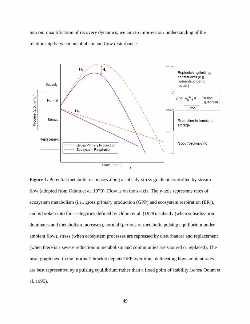
49

into our quantification of recovery dynamics, we aim to improve our understanding of the

relationship between metabolism and flow disturbance.

Figure 1. Potential metabolic responses along a subsidy-stress gradient controlled by stream

flow (adopted from Odum et al. 1979). Flow is on the x-axis. The y-axis represents rates of

ecosystem metabolism (i.e., gross primary production (GPP) and ecosystem respiration (ER)),

and is broken into four categories defined by Odum et al. (1979): subsidy (when subsidization

dominates and metabolism increases), normal (periods of metabolic pulsing equilibrium under

ambient flow), stress (when ecosystem processes are repressed by disturbance) and replacement

(when there is a severe reduction in metabolism and communities are scoured or replaced). The

inset graph next to the ‘normal’ bracket depicts GPP over time, delineating how ambient rates

are best represented by a pulsing equilibrium rather than a fixed point of stability (sensu Odum et

al. 1995).

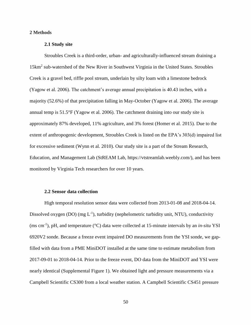
50

2 Methods

2.1 Study site

Stroubles Creek is a third-order, urban- and agriculturally-influenced stream draining a

15km2 sub-watershed of the New River in Southwest Virginia in the United States. Stroubles

Creek is a gravel bed, riffle pool stream, underlain by silty loam with a limestone bedrock

(Yagow et al. 2006). The catchment’s average annual precipitation is 40.43 inches, with a

majority (52.6%) of that precipitation falling in May-October (Yagow et al. 2006). The average

annual temp is 51.5°F (Yagow et al. 2006). The catchment draining into our study site is

approximately 87% developed, 11% agriculture, and 3% forest (Homer et al. 2015). Due to the

extent of anthropogenic development, Stroubles Creek is listed on the EPA’s 303(d) impaired list

for excessive sediment (Wynn et al. 2010). Our study site is a part of the Stream Research,

Education, and Management Lab (StREAM Lab, https://vtstreamlab.weebly.com/), and has been

monitored by Virginia Tech researchers for over 10 years.

2.2 Sensor data collection

High temporal resolution sensor data were collected from 2013-01-08 and 2018-04-14.

Dissolved oxygen (DO) (mg L-1), turbidity (nephelometric turbidity unit, NTU), conductivity

(ms cm-1), pH, and temperature (°C) data were collected at 15-minute intervals by an in-situ YSI

6920V2 sonde. Because a freeze event impaired DO measurements from the YSI sonde, we gap-

filled with data from a PME MiniDOT installed at the same time to estimate metabolism from

2017-09-01 to 2018-04-14. Prior to the freeze event, DO data from the MiniDOT and YSI were

nearly identical (Supplemental Figure 1). We obtained light and pressure measurements via a

Campbell Scientific CS300 from a local weather station. A Campbell Scientific CS451 pressure

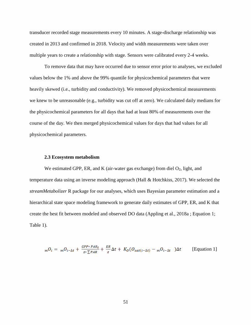
51

transducer recorded stage measurements every 10 minutes. A stage-discharge relationship was

created in 2013 and confirmed in 2018. Velocity and width measurements were taken over

multiple years to create a relationship with stage. Sensors were calibrated every 2-4 weeks.

To remove data that may have occurred due to sensor error prior to analyses, we excluded

values below the 1% and above the 99% quantile for physicochemical parameters that were

heavily skewed (i.e., turbidity and conductivity). We removed physicochemical measurements

we knew to be unreasonable (e.g., turbidity was cut off at zero). We calculated daily medians for

the physicochemical parameters for all days that had at least 80% of measurements over the

course of the day. We then merged physicochemical values for days that had values for all

physicochemical parameters.

2.3 Ecosystem metabolism

We estimated GPP, ER, and K (air-water gas exchange) from diel O2, light, and

temperature data using an inverse modeling approach (Hall & Hotchkiss, 2017). We selected the

streamMetabolizer R package for our analyses, which uses Bayesian parameter estimation and a

hierarchical state space modeling framework to generate daily estimates of GPP, ER, and K that

create the best fit between modeled and observed DO data (Appling et al., 2018a ; Equation 1;

Table 1).

[Equation 1]

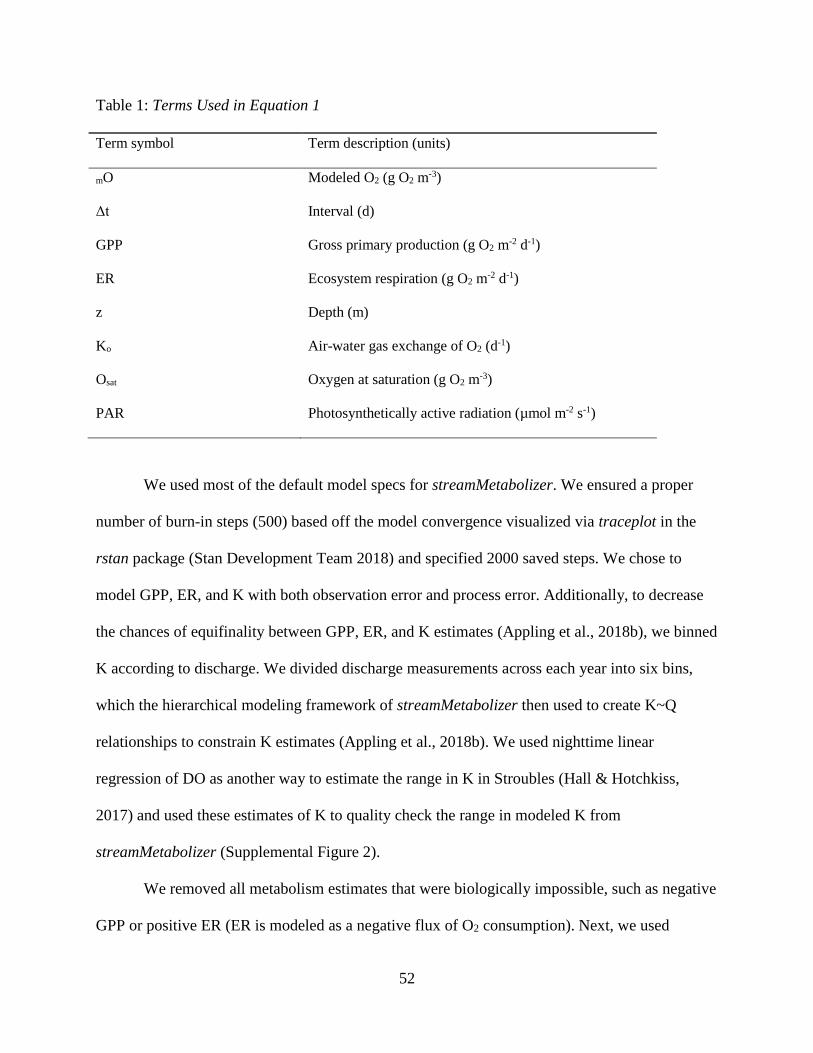
52

Table 1: Terms Used in Equation 1

Term symbol Term description (units)

mO Modeled O2 (g O2 m-3)

Δt Interval (d)

GPP Gross primary production (g O2 m-2 d-1)

ER Ecosystem respiration (g O2 m-2 d-1)

z Depth (m)

Ko Air-water gas exchange of O2 (d-1)

Osat Oxygen at saturation (g O2 m-3)

PAR Photosynthetically active radiation (µmol m-2 s-1)

We used most of the default model specs for streamMetabolizer. We ensured a proper

number of burn-in steps (500) based off the model convergence visualized via traceplot in the

rstan package (Stan Development Team 2018) and specified 2000 saved steps. We chose to

model GPP, ER, and K with both observation error and process error. Additionally, to decrease

the chances of equifinality between GPP, ER, and K estimates (Appling et al., 2018b), we binned

K according to discharge. We divided discharge measurements across each year into six bins,

which the hierarchical modeling framework of streamMetabolizer then used to create K~Q

relationships to constrain K estimates (Appling et al., 2018b). We used nighttime linear

regression of DO as another way to estimate the range in K in Stroubles (Hall & Hotchkiss,

2017) and used these estimates of K to quality check the range in modeled K from

streamMetabolizer (Supplemental Figure 2).

We removed all metabolism estimates that were biologically impossible, such as negative

GPP or positive ER (ER is modeled as a negative flux of O2 consumption). Next, we used

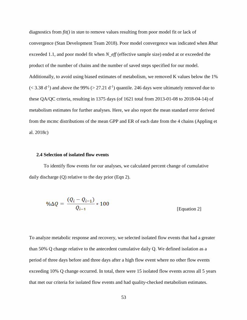
53

diagnostics from fit() in stan to remove values resulting from poor model fit or lack of

convergence (Stan Development Team 2018). Poor model convergence was indicated when Rhat

exceeded 1.1, and poor model fit when N_eff (effective sample size) ended at or exceeded the

product of the number of chains and the number of saved steps specified for our model.

Additionally, to avoid using biased estimates of metabolism, we removed K values below the 1%

(< 3.38 d-1) and above the 99% (> 27.21 d-1) quantile. 246 days were ultimately removed due to

these QA/QC criteria, resulting in 1375 days (of 1621 total from 2013-01-08 to 2018-04-14) of

metabolism estimates for further analyses. Here, we also report the mean standard error derived

from the mcmc distributions of the mean GPP and ER of each date from the 4 chains (Appling et

al. 2018c)

2.4 Selection of isolated flow events

To identify flow events for our analyses, we calculated percent change of cumulative

daily discharge (Q) relative to the day prior (Eqn 2).

[Equation 2]

To analyze metabolic response and recovery, we selected isolated flow events that had a greater

than 50% Q change relative to the antecedent cumulative daily Q. We defined isolation as a

period of three days before and three days after a high flow event where no other flow events

exceeding 10% Q change occurred. In total, there were 15 isolated flow events across all 5 years

that met our criteria for isolated flow events and had quality-checked metabolism estimates.

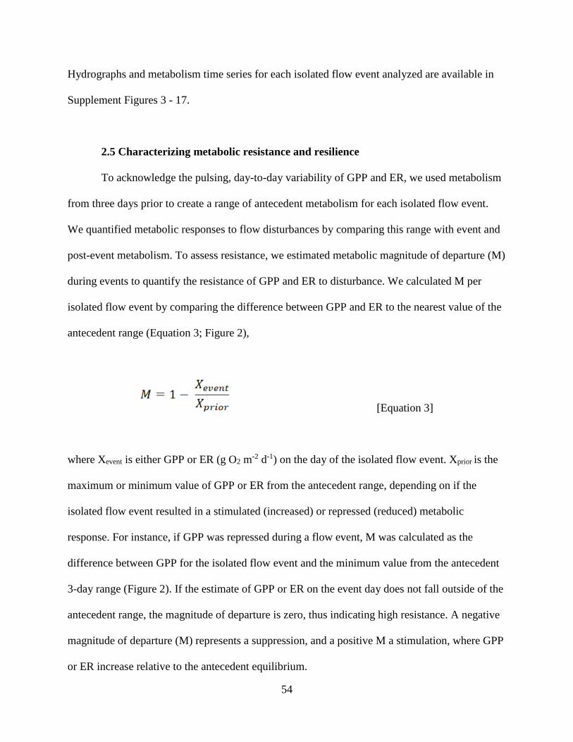
54

Hydrographs and metabolism time series for each isolated flow event analyzed are available in

Supplement Figures 3 - 17.

2.5 Characterizing metabolic resistance and resilience

To acknowledge the pulsing, day-to-day variability of GPP and ER, we used metabolism

from three days prior to create a range of antecedent metabolism for each isolated flow event.

We quantified metabolic responses to flow disturbances by comparing this range with event and

post-event metabolism. To assess resistance, we estimated metabolic magnitude of departure (M)

during events to quantify the resistance of GPP and ER to disturbance. We calculated M per

isolated flow event by comparing the difference between GPP and ER to the nearest value of the

antecedent range (Equation 3; Figure 2),

[Equation 3]

where Xevent is either GPP or ER (g O2 m-2 d-1) on the day of the isolated flow event. Xprior is the

maximum or minimum value of GPP or ER from the antecedent range, depending on if the

isolated flow event resulted in a stimulated (increased) or repressed (reduced) metabolic

response. For instance, if GPP was repressed during a flow event, M was calculated as the

difference between GPP for the isolated flow event and the minimum value from the antecedent

3-day range (Figure 2). If the estimate of GPP or ER on the event day does not fall outside of the

antecedent range, the magnitude of departure is zero, thus indicating high resistance. A negative

magnitude of departure (M) represents a suppression, and a positive M a stimulation, where GPP

or ER increase relative to the antecedent equilibrium.

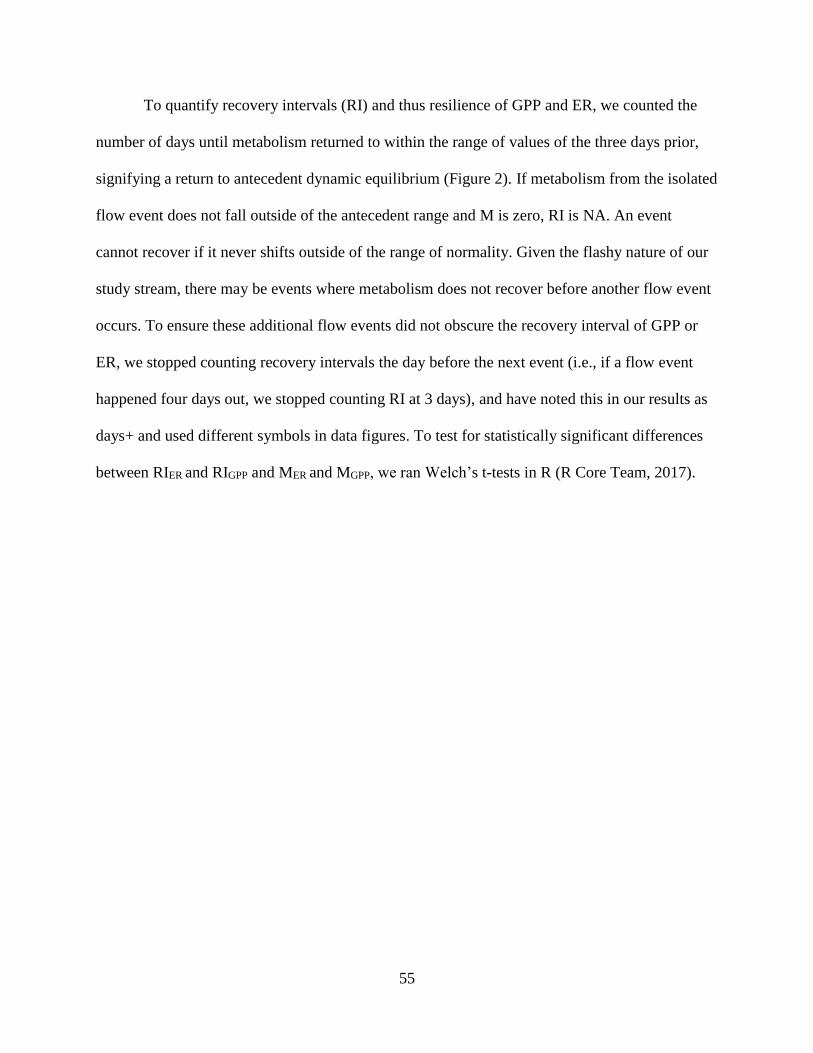
55

To quantify recovery intervals (RI) and thus resilience of GPP and ER, we counted the

number of days until metabolism returned to within the range of values of the three days prior,

signifying a return to antecedent dynamic equilibrium (Figure 2). If metabolism from the isolated

flow event does not fall outside of the antecedent range and M is zero, RI is NA. An event

cannot recover if it never shifts outside of the range of normality. Given the flashy nature of our

study stream, there may be events where metabolism does not recover before another flow event

occurs. To ensure these additional flow events did not obscure the recovery interval of GPP or

ER, we stopped counting recovery intervals the day before the next event (i.e., if a flow event

happened four days out, we stopped counting RI at 3 days), and have noted this in our results as

days+ and used different symbols in data figures. To test for statistically significant differences

between RIER and RIGPP and MER and MGPP, we ran Welch’s t-tests in R (R Core Team, 2017).

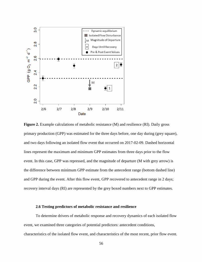
56

Figure 2. Example calculations of metabolic resistance (M) and resilience (RI). Daily gross

primary production (GPP) was estimated for the three days before, one day during (grey square),

and two days following an isolated flow event that occurred on 2017-02-09. Dashed horizontal

lines represent the maximum and minimum GPP estimates from three days prior to the flow

event. In this case, GPP was repressed, and the magnitude of departure (M with grey arrow) is

the difference between minimum GPP estimate from the antecedent range (bottom dashed line)

and GPP during the event. After this flow event, GPP recovered to antecedent range in 2 days;

recovery interval days (RI) are represented by the grey boxed numbers next to GPP estimates.

2.6 Testing predictors of metabolic resistance and resilience

To determine drivers of metabolic response and recovery dynamics of each isolated flow

event, we examined three categories of potential predictors: antecedent conditions,

characteristics of the isolated flow event, and characteristics of the most recent, prior flow event.

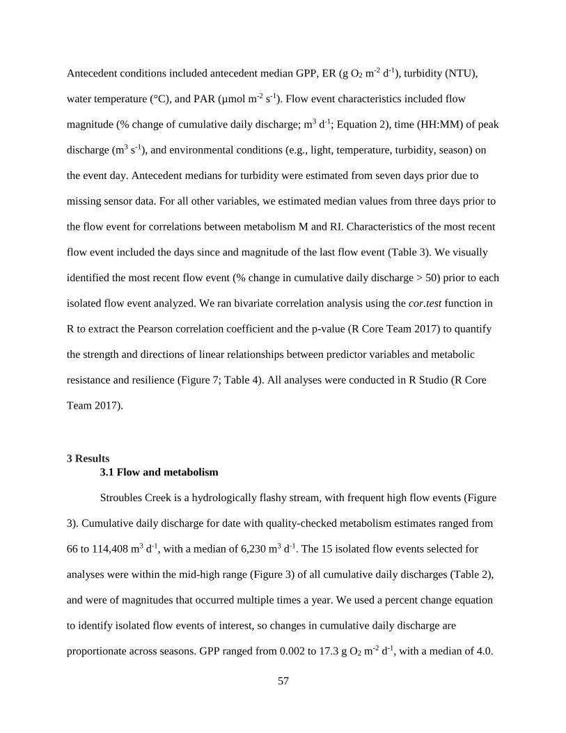
57

Antecedent conditions included antecedent median GPP, ER (g O2 m-2 d-1), turbidity (NTU),

water temperature (°C), and PAR (µmol m-2 s-1). Flow event characteristics included flow

magnitude (% change of cumulative daily discharge; m3 d-1; Equation 2), time (HH:MM) of peak

discharge (m3 s-1), and environmental conditions (e.g., light, temperature, turbidity, season) on

the event day. Antecedent medians for turbidity were estimated from seven days prior due to

missing sensor data. For all other variables, we estimated median values from three days prior to

the flow event for correlations between metabolism M and RI. Characteristics of the most recent

flow event included the days since and magnitude of the last flow event (Table 3). We visually

identified the most recent flow event (% change in cumulative daily discharge > 50) prior to each

isolated flow event analyzed. We ran bivariate correlation analysis using the cor.test function in

R to extract the Pearson correlation coefficient and the p-value (R Core Team 2017) to quantify

the strength and directions of linear relationships between predictor variables and metabolic

resistance and resilience (Figure 7; Table 4). All analyses were conducted in R Studio (R Core

Team 2017).

3 Results

3.1 Flow and metabolism

Stroubles Creek is a hydrologically flashy stream, with frequent high flow events (Figure

3). Cumulative daily discharge for date with quality-checked metabolism estimates ranged from

66 to 114,408 m3 d-1, with a median of 6,230 m3 d-1. The 15 isolated flow events selected for

analyses were within the mid-high range (Figure 3) of all cumulative daily discharges (Table 2),

and were of magnitudes that occurred multiple times a year. We used a percent change equation

to identify isolated flow events of interest, so changes in cumulative daily discharge are

proportionate across seasons. GPP ranged from 0.002 to 17.3 g O2 m-2 d-1, with a median of 4.0.

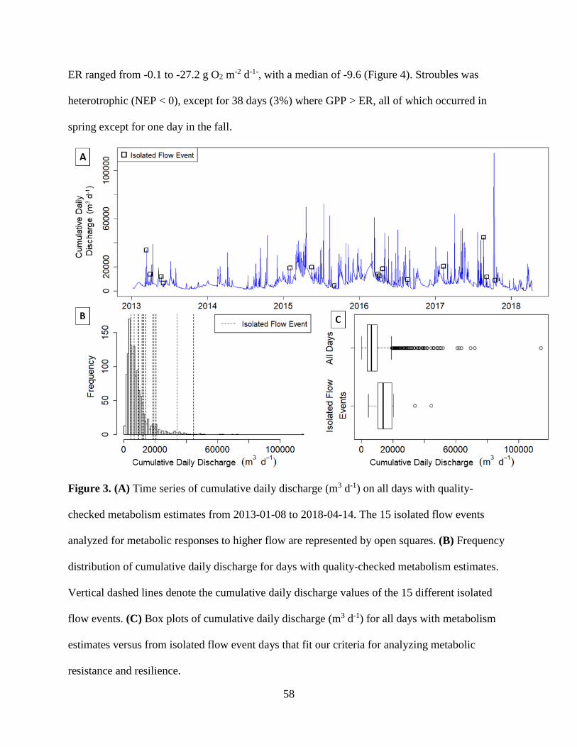
58

ER ranged from -0.1 to -27.2 g O2 m-2 d-1-, with a median of -9.6 (Figure 4). Stroubles was

heterotrophic (NEP < 0), except for 38 days (3%) where GPP > ER, all of which occurred in

spring except for one day in the fall.

Figure 3. (A) Time series of cumulative daily discharge (m3 d-1) on all days with quality-

checked metabolism estimates from 2013-01-08 to 2018-04-14. The 15 isolated flow events

analyzed for metabolic responses to higher flow are represented by open squares. (B) Frequency

distribution of cumulative daily discharge for days with quality-checked metabolism estimates.

Vertical dashed lines denote the cumulative daily discharge values of the 15 different isolated

flow events. (C) Box plots of cumulative daily discharge (m3 d-1) for all days with metabolism

estimates versus from isolated flow event days that fit our criteria for analyzing metabolic

resistance and resilience.

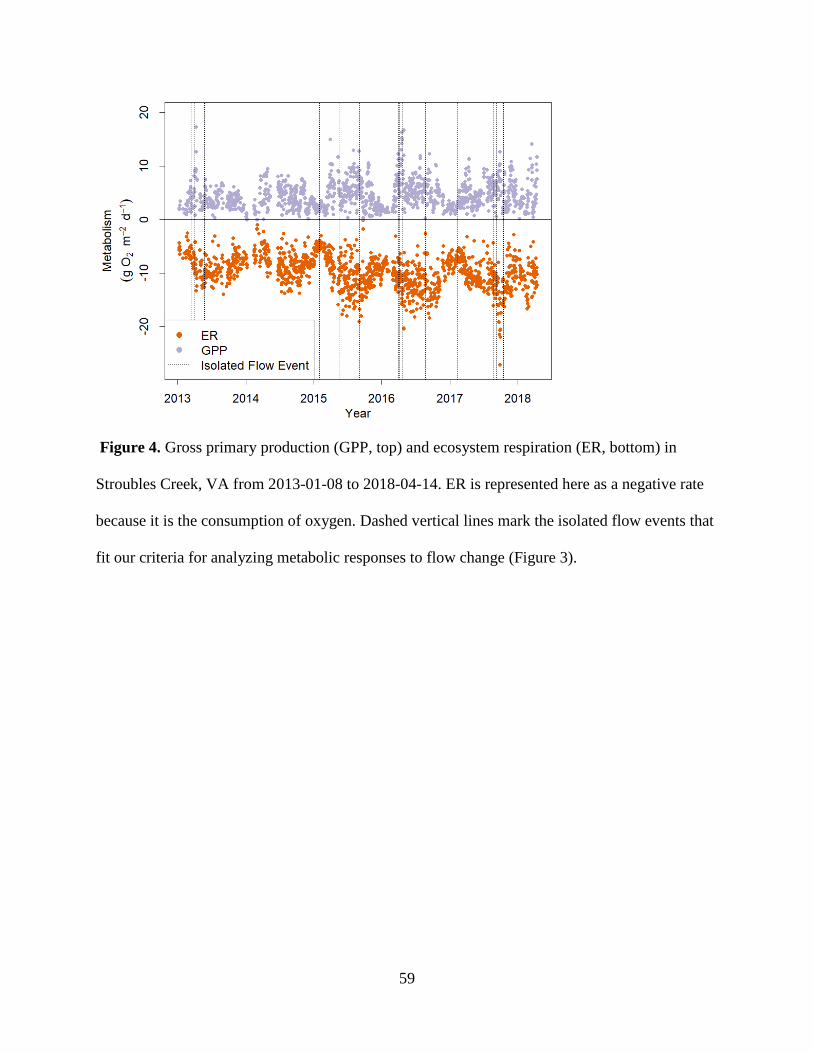
59

Figure 4. Gross primary production (GPP, top) and ecosystem respiration (ER, bottom) in

Stroubles Creek, VA from 2013-01-08 to 2018-04-14. ER is represented here as a negative rate

because it is the consumption of oxygen. Dashed vertical lines mark the isolated flow events that

fit our criteria for analyzing metabolic responses to flow change (Figure 3).

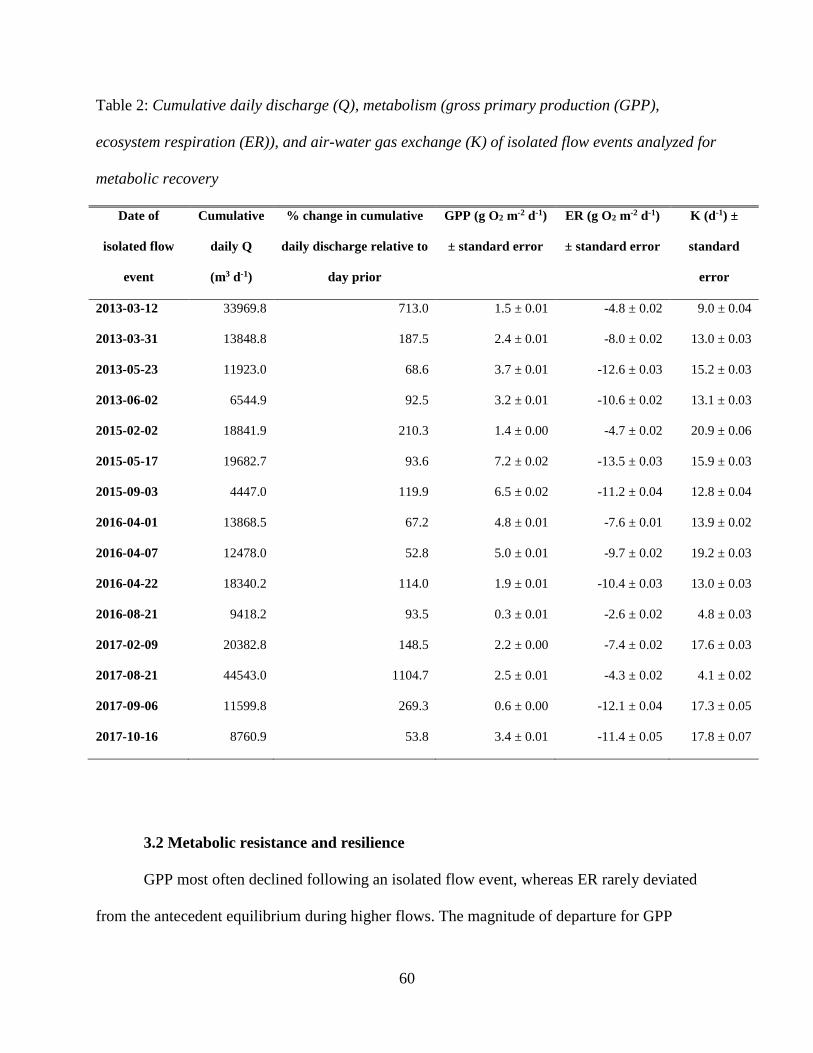
60

Table 2: Cumulative daily discharge (Q), metabolism (gross primary production (GPP),

ecosystem respiration (ER)), and air-water gas exchange (K) of isolated flow events analyzed for

metabolic recovery

Date of

isolated flow

event

Cumulative

daily Q

(m3 d-1)

% change in cumulative

daily discharge relative to

day prior

GPP (g O2 m-2 d-1)

± standard error

ER (g O2 m-2 d-1)

± standard error

K (d-1) ±

standard

error

2013-03-12 33969.8 713.0 1.5 ± 0.01 -4.8 ± 0.02 9.0 ± 0.04

2013-03-31 13848.8 187.5 2.4 ± 0.01 -8.0 ± 0.02 13.0 ± 0.03

2013-05-23 11923.0 68.6 3.7 ± 0.01 -12.6 ± 0.03 15.2 ± 0.03

2013-06-02 6544.9 92.5 3.2 ± 0.01 -10.6 ± 0.02 13.1 ± 0.03

2015-02-02 18841.9 210.3 1.4 ± 0.00 -4.7 ± 0.02 20.9 ± 0.06

2015-05-17 19682.7 93.6 7.2 ± 0.02 -13.5 ± 0.03 15.9 ± 0.03

2015-09-03 4447.0 119.9 6.5 ± 0.02 -11.2 ± 0.04 12.8 ± 0.04

2016-04-01 13868.5 67.2 4.8 ± 0.01 -7.6 ± 0.01 13.9 ± 0.02

2016-04-07 12478.0 52.8 5.0 ± 0.01 -9.7 ± 0.02 19.2 ± 0.03

2016-04-22 18340.2 114.0 1.9 ± 0.01 -10.4 ± 0.03 13.0 ± 0.03

2016-08-21 9418.2 93.5 0.3 ± 0.01 -2.6 ± 0.02 4.8 ± 0.03

2017-02-09 20382.8 148.5 2.2 ± 0.00 -7.4 ± 0.02 17.6 ± 0.03

2017-08-21 44543.0 1104.7 2.5 ± 0.01 -4.3 ± 0.02 4.1 ± 0.02

2017-09-06 11599.8 269.3 0.6 ± 0.00 -12.1 ± 0.04 17.3 ± 0.05

2017-10-16 8760.9 53.8 3.4 ± 0.01 -11.4 ± 0.05 17.8 ± 0.07

3.2 Metabolic resistance and resilience

GPP most often declined following an isolated flow event, whereas ER rarely deviated

from the antecedent equilibrium during higher flows. The magnitude of departure for GPP

61

(MGPP) ranged from -0.92 to 0.09, with a median of -0.14 (Table 3; Figure 6). GPP was inhibited

in 11 of 15 analyzed isolated flow events, and stimulated during two events. The magnitude of

departure for ER (MER) ranged from -0.59 to 0.22, with a median of 0. There were 3 of 15

analyzed isolated flow events that stimulated ER, 5 that resulted in repression of ER, and 7

events where ER did not deviate from the antecedent equilibrium (i.e., MER was 0). Overall, the

direction of ER response to elevated flow was more variable than that of GPP.

Although GPP exhibited stronger responses across isolated flow events than ER, MGPP

and MER were positively correlated (R2 = 0.39, p = 0.007, Figure 6) and not significantly

different (p = 0.06, α = 0.05). MGPP was less than MER for nearly all of the isolated flow events,

except for one event in which MGPP and MER were both zero, and two events where both MGPP

and MER were small. The isolated flow event that induced the greatest stimulation of GPP (MGPP

= 0.09) also stimulated ER (MER = 0.05). The other two events that stimulated ER had no

response from GPP (MGPP = 0) or had a minor GPP reduction (MGPP = -0.06). Similarly, the only

other event that stimulated GPP (MGPP = 0.03) had no ER response, suggesting that stimulation

may cause a minor, brief decoupling between GPP and ER at our study site.

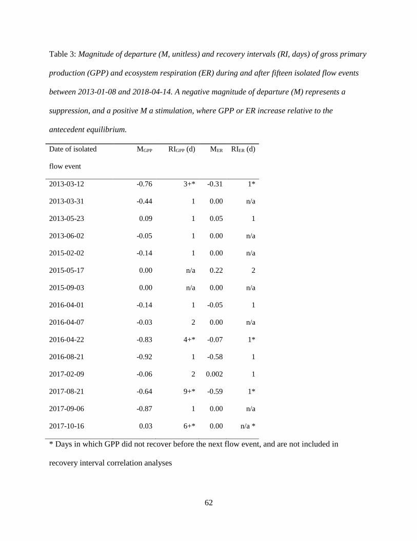
62

Table 3: Magnitude of departure (M, unitless) and recovery intervals (RI, days) of gross primary

production (GPP) and ecosystem respiration (ER) during and after fifteen isolated flow events

between 2013-01-08 and 2018-04-14. A negative magnitude of departure (M) represents a

suppression, and a positive M a stimulation, where GPP or ER increase relative to the

antecedent equilibrium.

Date of isolated

flow event

MGPP RIGPP (d) MER RIER (d)

2013-03-12 -0.76 3+* -0.31 1*

2013-03-31 -0.44 1 0.00 n/a

2013-05-23 0.09 1 0.05 1

2013-06-02 -0.05 1 0.00 n/a

2015-02-02 -0.14 1 0.00 n/a

2015-05-17 0.00 n/a 0.22 2

2015-09-03 0.00 n/a 0.00 n/a

2016-04-01 -0.14 1 -0.05 1

2016-04-07 -0.03 2 0.00 n/a

2016-04-22 -0.83 4+* -0.07 1*

2016-08-21 -0.92 1 -0.58 1

2017-02-09 -0.06 2 0.002 1

2017-08-21 -0.64 9+* -0.59 1*

2017-09-06 -0.87 1 0.00 n/a

2017-10-16 0.03 6+* 0.00 n/a *

* Days in which GPP did not recover before the next flow event, and are not included in

recovery interval correlation analyses

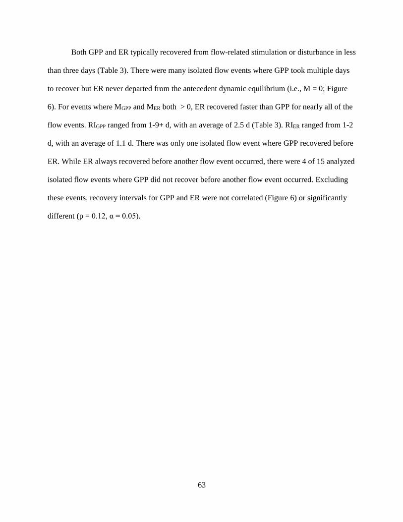
63

Both GPP and ER typically recovered from flow-related stimulation or disturbance in less

than three days (Table 3). There were many isolated flow events where GPP took multiple days

to recover but ER never departed from the antecedent dynamic equilibrium (i.e., M = 0; Figure

6). For events where MGPP and MER both > 0, ER recovered faster than GPP for nearly all of the

flow events. RIGPP ranged from 1-9+ d, with an average of 2.5 d (Table 3). RIER ranged from 1-2

d, with an average of 1.1 d. There was only one isolated flow event where GPP recovered before

ER. While ER always recovered before another flow event occurred, there were 4 of 15 analyzed

isolated flow events where GPP did not recover before another flow event occurred. Excluding

these events, recovery intervals for GPP and ER were not correlated (Figure 6) or significantly

different (p = 0.12, α = 0.05).

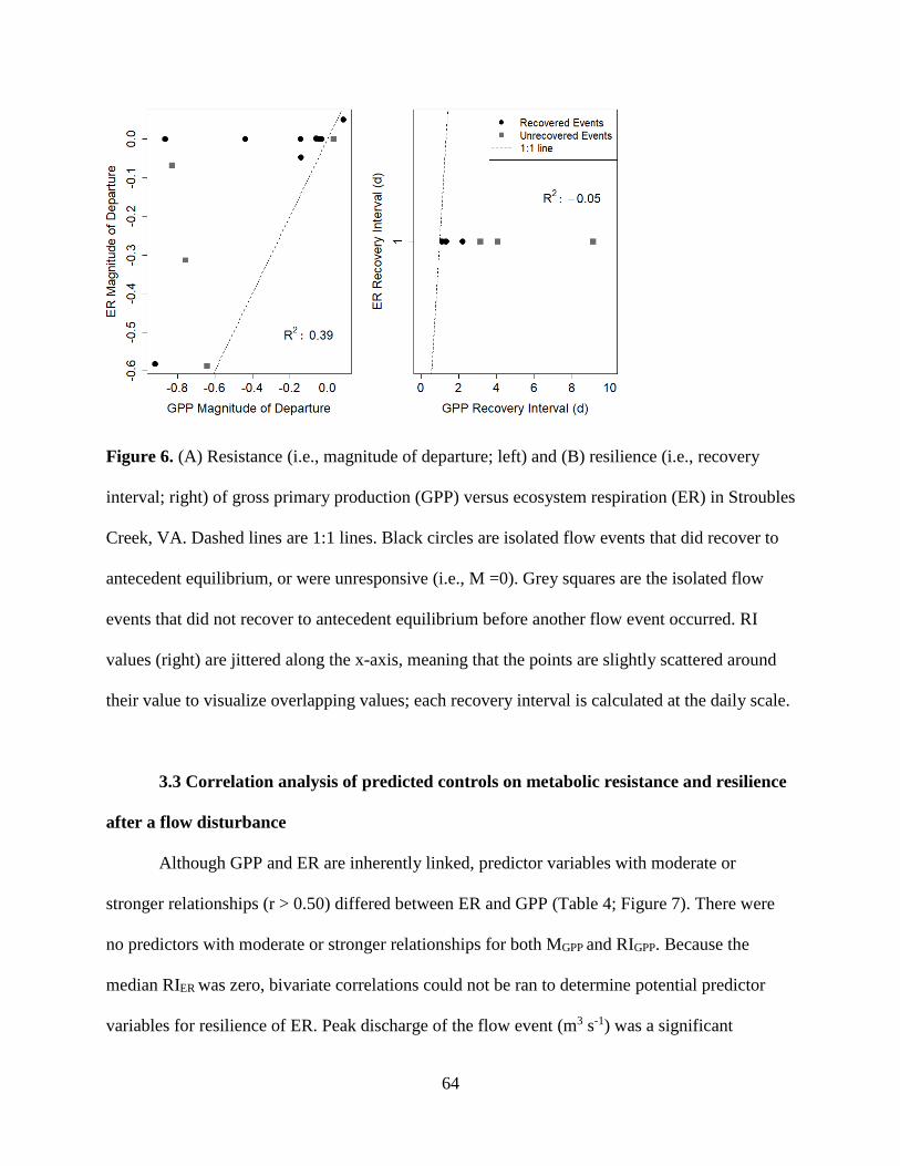
64

Figure 6. (A) Resistance (i.e., magnitude of departure; left) and (B) resilience (i.e., recovery

interval; right) of gross primary production (GPP) versus ecosystem respiration (ER) in Stroubles

Creek, VA. Dashed lines are 1:1 lines. Black circles are isolated flow events that did recover to

antecedent equilibrium, or were unresponsive (i.e., M =0). Grey squares are the isolated flow

events that did not recover to antecedent equilibrium before another flow event occurred. RI

values (right) are jittered along the x-axis, meaning that the points are slightly scattered around

their value to visualize overlapping values; each recovery interval is calculated at the daily scale.

3.3 Correlation analysis of predicted controls on metabolic resistance and resilience

after a flow disturbance

Although GPP and ER are inherently linked, predictor variables with moderate or

stronger relationships (r > 0.50) differed between ER and GPP (Table 4; Figure 7). There were

no predictors with moderate or stronger relationships for both MGPP and RIGPP. Because the

median RIER was zero, bivariate correlations could not be ran to determine potential predictor

variables for resilience of ER. Peak discharge of the flow event (m3 s-1) was a significant

65

predictor of MER (r = -0.59). The magnitude of each disturbance, characterized by the % change

in cumulative daily discharge, was negatively correlated with MGPP (r = -0.46, p = 0.08) and

significantly negatively correlated with MER (r = 0.66, p = 0.01, α = 0.05) (Figure 8), but was not

significantly correlated with RIGPP (p = 0.54; α = 0.05). Overall, there were multiple

environmental controls on metabolic resistance or resilience that were strongly correlated with

either GPP or ER, but no significant drivers of both GPP and ER resistance and resilience.

66

Table 4: Pearson correlations (r) between predicted drivers of gross primary production (GPP)

and ecosystem respiration (ER) magnitudes of departure (M) and recovery intervals (RI) of

isolated flow events. Predictor variables with moderate or stronger relationships (r > 0.50) are

bolded.

Predictor variables (units) RIGPP r MGPP r RIER r MER r

Isolated flow event of interest

Daily median PAR (µmol m-2 s-1) -0.26 0.16 n/a -0.17

Daily peak discharge (m3 s-1) -0.03 -0.32 n/a -0.59

Daily median temperature (°C) -0.46 -0.11 n/a -0.28

Event median discharge (m3 s-1) 0.00 -0.21 n/a 0.03

% discharge change during event -0.24 -0.46 n/a -0.66

Season -0.42 -0.16 n/a -0.18

Time of peak discharge (HH:MM) -0.65 -0.12 n/a -0.10

Turbidity (NTU) -0.21 -0.41 n/a -0.18

Most recent flow event

Days since last event (d) 0.23 0.15 n/a 0.10

Last event cumulative daily discharge (m3 d-1) 0.59 0.40 n/a 0.21

% discharge change of last event 0.55 0.51 n/a 0.47

Antecedent conditions

Antecedent median K (d-1) 0.26 -0.04 n/a -0.08

Antecedent GPP (g O2 m-2 d-1) 0.02 -0.48 n/a -0.12

Antecedent ER (g O2 m-2 d-1) 0.16 0.25 n/a 0.09

Antecedent median PAR (µmol m-2 s-1) -0.31 0.12 n/a 0.04

Antecedent median discharge (m3 s-1) 0.08 0.34 n/a 0.40

Antecedent median water temperature (°C) -0.32 -0.14 n/a -0.29

Antecedent median turbidity (NTU) -0.23 0.13 n/a 0.00

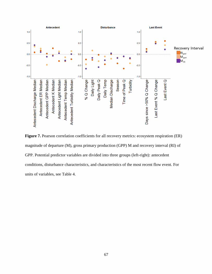
67

Figure 7. Pearson correlation coefficients for all recovery metrics: ecosystem respiration (ER)

magnitude of departure (M), gross primary production (GPP) M and recovery interval (RI) of

GPP. Potential predictor variables are divided into three groups (left-right): antecedent

conditions, disturbance characteristics, and characteristics of the most recent flow event. For

units of variables, see Table 4.

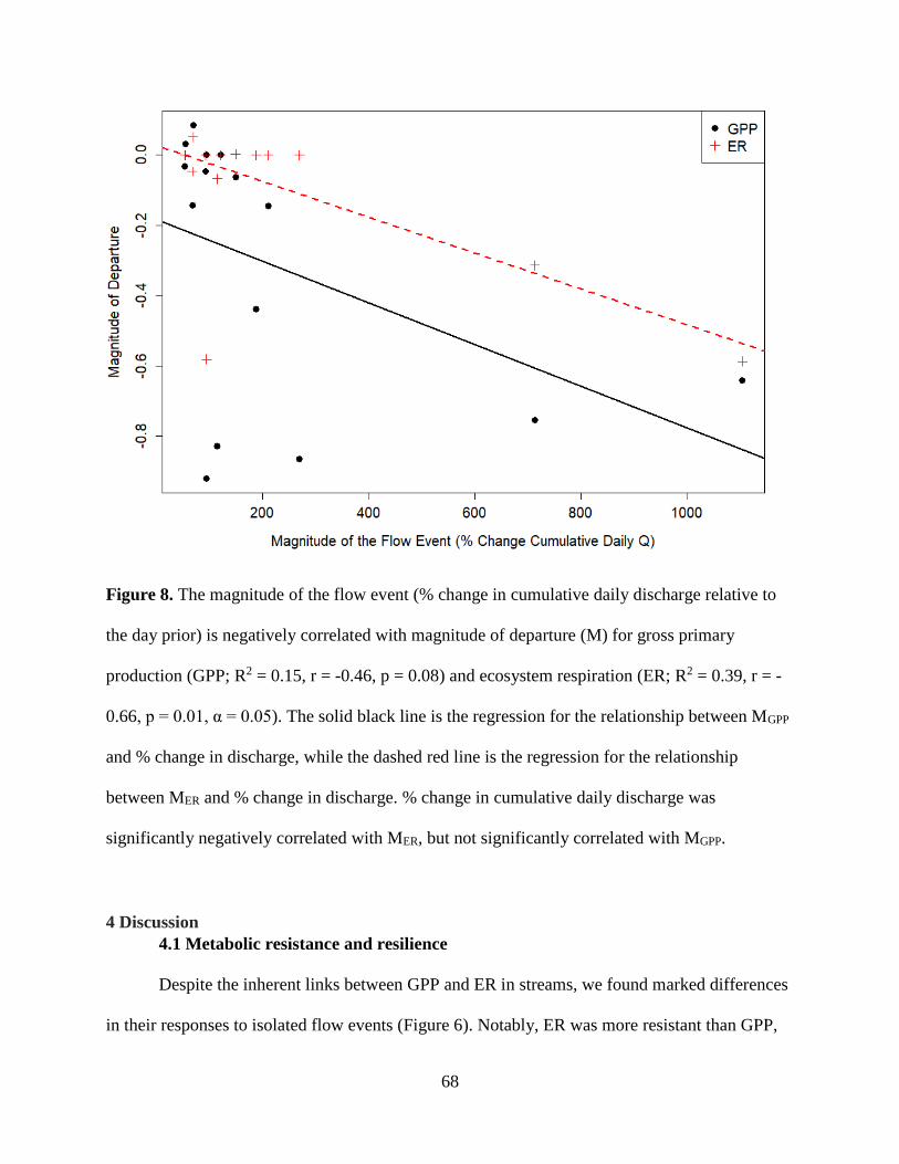
68

Figure 8. The magnitude of the flow event (% change in cumulative daily discharge relative to

the day prior) is negatively correlated with magnitude of departure (M) for gross primary

production (GPP; R2 = 0.15, r = -0.46, p = 0.08) and ecosystem respiration (ER; R2 = 0.39, r = -

0.66, p = 0.01, α = 0.05). The solid black line is the regression for the relationship between MGPP

and % change in discharge, while the dashed red line is the regression for the relationship

between MER and % change in discharge. % change in cumulative daily discharge was

significantly negatively correlated with MER, but not significantly correlated with MGPP.

4 Discussion

4.1 Metabolic resistance and resilience

Despite the inherent links between GPP and ER in streams, we found marked differences

in their responses to isolated flow events (Figure 6). Notably, ER was more resistant than GPP,

69

supporting our first hypothesis (Figure 1). For many of the events analyzed, ER did not shift out

of the range of antecedent equilibrium (i.e., M = 0), whereas GPP was reduced (Figure 6; Table

3). Decreased GPP can decrease ER because autotrophs respire and also provide a labile organic

matter (OM) source for heterotroph growth and respiration (Kaplan and Bott 1982, Uehlinger

and Naegeli 1998). Yet, the potential negative consequences of flow on heterotrophic activity are

balanced with the possibility for flow-induced stimulation of respiration caused by increased

DOC concentrations from allochthonous sources (Demars 2018), more labile DOC (Mulholland

et al. 1990). Further, GPP can be stimulated via influxes of limiting nutrients (Beaulieu et al.

2013). However, in our study system, three events stimulated ER, whereas there were two

instances of minor GPP stimulation (Table 3). Flow-induced stimulation of GPP may have been

caused by the replenishment of a limiting nutrient (Lamberti and Steinman 1997).

ER was also more resilient than GPP. Across all flow events, ER recovered on average

much faster than GPP (Table 3; Figure 6). ER returned to antecedent rates within one day after

flow events for all but one event, whereas GPP recovery ranged from 1-9+ days. Resilience

differences between ER and GPP (i.e., RIER and RIGPP) are likely a result of flow-induced

changes to physicochemical parameters (e.g., turbidity), which can alter GPP more than the

impacts of flow would alone (O’Donnell & Hotchkiss, in review). For instance, sustained periods

of high turbidity following a disturbance can prolong the recovery of GPP by inhibiting light

attenuation (Blaszczak et al. 2018). In contrast, faster average resilience of ER is likely a

function of both OM stimulation of ER, and the greater resistance of ER to disturbances (i.e.,

smaller M; Table 3). The greater resistance of ER to disturbances indicates potentially less

biomass scoured than primary producers, and therefore more capacity for greater resilience (i.e.,

smaller RI). The correlation of MGPP and MER, but a lack of correlation between RIGPP and RIER

70

(Figure 6), suggests that the instantaneous responses of GPP and ER to flow disturbances align,

while metabolism becomes temporarily decoupled while recovering. Ultimately, flow-induced

changes can disproportionately negatively impact GPP relative to ER.

4.2 Controls on metabolic resistance and resilience following a flow event

The characteristics of a flow disturbance (i.e., % change in cumulative daily discharge,

larger peak event discharge) were significantly related to MER but not MGPP, suggesting that

while GPP may respond similarly to flows regardless of magnitude, ER has greater resistance to

flows of smaller magnitudes. Our hypothesis that isolated flow events of greater magnitudes (i.e.,

larger % change in cumulative daily discharge) would result in less resistance and a higher MGPP

and MER due to increased scouring was supported only for MER. Flow events of greater

magnitude were weakly correlated with MGPP (r = -0.46; Table 4; Figure 8), supporting the idea

that GPP may have low resistance to flow disturbances, regardless of magnitude (Reisinger et al.

2017; Roley et al. 2014). The different responses of GPP and ER to variable flow can potentially

be attributed to the differences in energy source and residence within the streambed of the

autotrophs and heterotrophs (Uehlinger 2000, 2006). The surface of the stream bed is dominated

by primary producers who reside in exposed areas because of their need for light for

photosynthesis. The exposed surfaces are more vulnerable to scour than the locations of the

heterotrophic biofilms tucked within, and protected by, the substrata and hyporheic zone

(Uehlinger 2000). However, higher flows may reduce metabolism in deeper sediments. Indeed,

MER was significantly negatively correlated with % change in cumulative daily discharge (r = -

0.66, p = 0.01; Figure 8). We tried to examine the effect of four of the five flow characteristics

defined by Poff et al. (1997) (magnitude, frequency, rate of change, timing; Table 2; Fig 5), yet

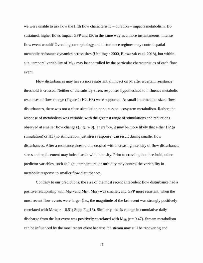
71

we were unable to ask how the fifth flow characteristic – duration – impacts metabolism. Do

sustained, higher flows impact GPP and ER in the same way as a more instantaneous, intense

flow event would? Overall, geomorphology and disturbance regimes may control spatial

metabolic resistance dynamics across sites (Uehlinger 2000, Blaszczak et al. 2018), but within-

site, temporal variability of MER may be controlled by the particular characteristics of each flow

event.

Flow disturbances may have a more substantial impact on M after a certain resistance

threshold is crossed. Neither of the subsidy-stress responses hypothesized to influence metabolic

responses to flow change (Figure 1; H2, H3) were supported. At small-intermediate sized flow

disturbances, there was not a clear stimulation nor stress on ecosystem metabolism. Rather, the

response of metabolism was variable, with the greatest range of stimulations and reductions

observed at smaller flow changes (Figure 8). Therefore, it may be more likely that either H2 (a

stimulation) or H3 (no stimulation, just stress response) can result during smaller flow

disturbances. After a resistance threshold is crossed with increasing intensity of flow disturbance,

stress and replacement may indeed scale with intensity. Prior to crossing that threshold, other

predictor variables, such as light, temperature, or turbidity may control the variability in

metabolic response to smaller flow disturbances.

Contrary to our predictions, the size of the most recent antecedent flow disturbance had a

positive relationship with MGPP and MER. MGPP was smaller, and GPP more resistant, when the

most recent flow events were larger (i.e., the magnitude of the last event was strongly positively

correlated with MGPP; r = 0.51; Supp Fig 18). Similarly, the % change in cumulative daily

discharge from the last event was positively correlated with MER (r = 0.47). Stream metabolism

can be influenced by the most recent event because the stream may still be recovering and

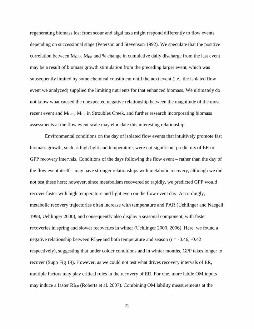
72

regenerating biomass lost from scour and algal taxa might respond differently to flow events

depending on successional stage (Peterson and Stevenson 1992). We speculate that the positive

correlation between MGPP, MER and % change in cumulative daily discharge from the last event

may be a result of biomass growth stimulation from the preceding larger event, which was

subsequently limited by some chemical constituent until the next event (i.e., the isolated flow

event we analyzed) supplied the limiting nutrients for that enhanced biomass. We ultimately do

not know what caused the unexpected negative relationship between the magnitude of the most

recent event and MGPP, MER in Stroubles Creek, and further research incorporating biomass

assessments at the flow event scale may elucidate this interesting relationship.

Environmental conditions on the day of isolated flow events that intuitively promote fast

biomass growth, such as high light and temperature, were not significant predictors of ER or

GPP recovery intervals. Conditions of the days following the flow event – rather than the day of

the flow event itself – may have stronger relationships with metabolic recovery, although we did

not test these here; however, since metabolism recovered so rapidly, we predicted GPP would

recover faster with high temperature and light even on the flow event day. Accordingly,

metabolic recovery trajectories often increase with temperature and PAR (Uehlinger and Naegeli

1998, Uehlinger 2000), and consequently also display a seasonal component, with faster

recoveries in spring and slower recoveries in winter (Uehlinger 2000, 2006). Here, we found a

negative relationship between RIGPP and both temperature and season (r = -0.46, -0.42

respectively), suggesting that under colder conditions and in winter months, GPP takes longer to

recover (Supp Fig 19). However, as we could not test what drives recovery intervals of ER,

multiple factors may play critical roles in the recovery of ER. For one, more labile OM inputs

may induce a faster RIER (Roberts et al. 2007). Combining OM lability measurements at the

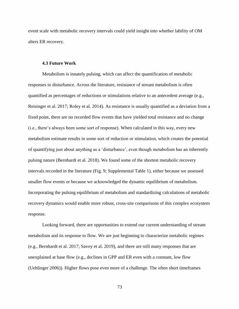
73

event scale with metabolic recovery intervals could yield insight into whether lability of OM

alters ER recovery.

4.3 Future Work

Metabolism is innately pulsing, which can affect the quantification of metabolic

responses to disturbance. Across the literature, resistance of stream metabolism is often

quantified as percentages of reductions or stimulations relative to an antecedent average (e.g.,

Reisinger et al. 2017; Roley et al. 2014). As resistance is usually quantified as a deviation from a

fixed point, there are no recorded flow events that have yielded total resistance and no change

(i.e., there’s always been some sort of response). When calculated in this way, every new

metabolism estimate results in some sort of reduction or stimulation, which creates the potential

of quantifying just about anything as a ‘disturbance’, even though metabolism has an inherently

pulsing nature (Bernhardt et al. 2018). We found some of the shortest metabolic recovery

intervals recorded in the literature (Fig. 9; Supplemental Table 1), either because we assessed

smaller flow events or because we acknowledged the dynamic equilibrium of metabolism.

Incorporating the pulsing equilibrium of metabolism and standardizing calculations of metabolic

recovery dynamics would enable more robust, cross-site comparisons of this complex ecosystem

response.

Looking forward, there are opportunities to extend our current understanding of stream

metabolism and its response to flow. We are just beginning to characterize metabolic regimes

(e.g., Bernhardt et al. 2017; Savoy et al. 2019), and there are still many responses that are

unexplained at base flow (e.g., declines in GPP and ER even with a constant, low flow

(Uehlinger 2006)). Higher flows pose even more of a challenge. The often short timeframes

74

between high flow events make isolating and quantifying their functional response very difficult.

As records of metabolic data sets increase and modeling tools improve, however, we may be able

to find enough isolated events to discern patterns, even potentially assessing impacts of multiple,

sequential high flow disturbances that did not meet our criteria for isolation.

Land use, geomorphology, and disturbance regime may affect site differences in

metabolic resistance and resilience (Figure 9; Supplemental Table 1; Uehlinger 2000, Blaszczak

et al. 2018). Limiting constituents have the potential to drive resilience, as high inputs of

otherwise limiting nutrients from agricultural fields or DOC from wetland rich areas may help

induce faster metabolic recovery (Uehlinger 2006). Sites that have more extensive hyporheic

zones, and thus more refugia for heterotrophs, may be more resistant to flow disturbances,

although this merits further research (Uehlinger 2000). Additionally, reaches that have access to

their floodplains may display less response from GPP and ER, as floodplains may mitigate the

role that extreme flow events play in regulating metabolism (Roley et al. 2014). As sensors

become cheaper and modeling software increasingly accessible, more long term, high frequency

datasets of metabolism estimates will be generated. Such data offers new opportunities to

understand both within- and across-site controls on metabolic resistance and resilience.

Consequently, although characterizing metabolic flow regimes may become easier,

understanding metabolic response to flow disturbances still poses a unique challenge.

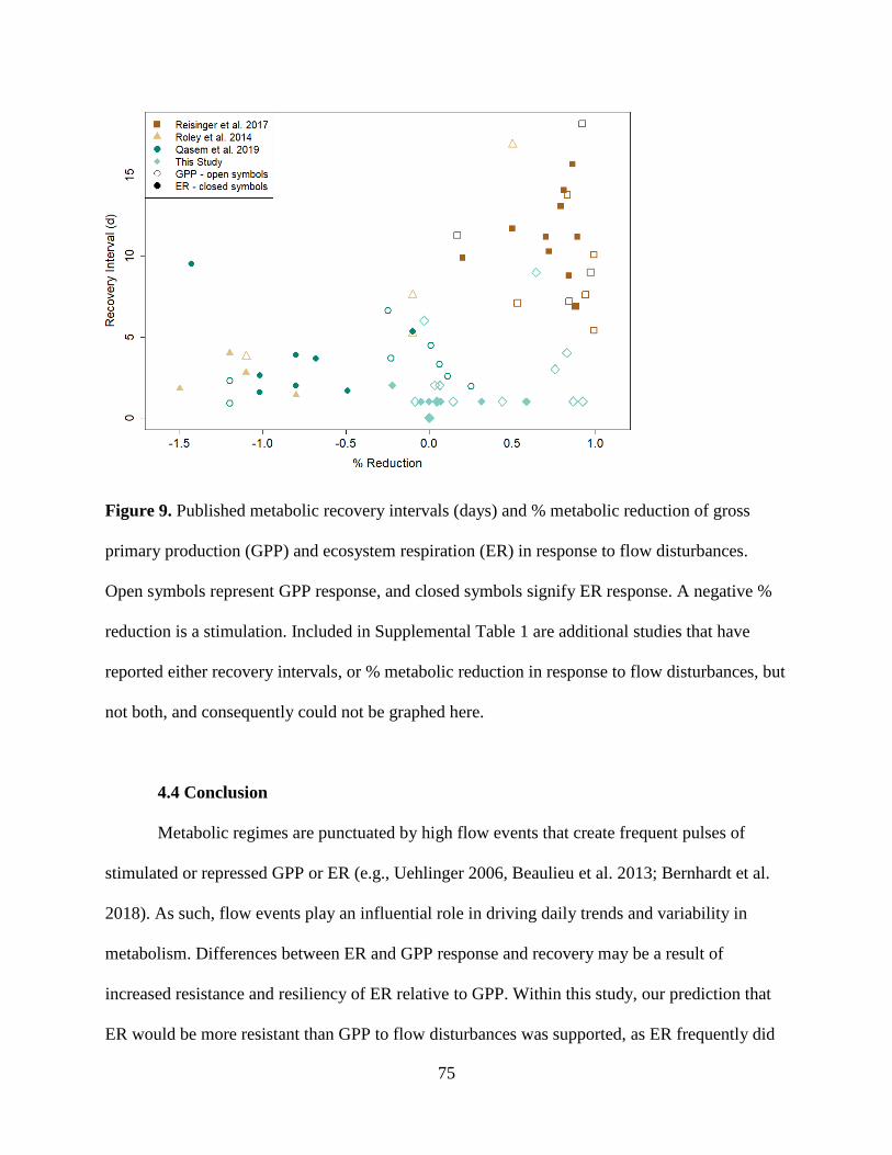
75

Figure 9. Published metabolic recovery intervals (days) and % metabolic reduction of gross

primary production (GPP) and ecosystem respiration (ER) in response to flow disturbances.

Open symbols represent GPP response, and closed symbols signify ER response. A negative %

reduction is a stimulation. Included in Supplemental Table 1 are additional studies that have

reported either recovery intervals, or % metabolic reduction in response to flow disturbances, but

not both, and consequently could not be graphed here.

4.4 Conclusion

Metabolic regimes are punctuated by high flow events that create frequent pulses of

stimulated or repressed GPP or ER (e.g., Uehlinger 2006, Beaulieu et al. 2013; Bernhardt et al.

2018). As such, flow events play an influential role in driving daily trends and variability in

metabolism. Differences between ER and GPP response and recovery may be a result of

increased resistance and resiliency of ER relative to GPP. Within this study, our prediction that

ER would be more resistant than GPP to flow disturbances was supported, as ER frequently did

76

not even deviate from the antecedent equilibrium (Table 3; Figure 6). However, ER had less

resistance to events of greater magnitude: MER had a negative, strong relationship with the %

discharge change of the flow event, whereas MGPP did not, suggesting that GPP responded

similarly to changes in flow regardless of flow magnitude (Figure 8). Metabolic response to

small and intermediate flow disturbances was variable, and resulted in both stimulations and

reductions in GPP and ER. Therefore, there may be a resistance threshold to flow disturbances,

where below this threshold other controls (light, season, or turbidity) might drive metabolic

response. Quantifying a resistance threshold of processes to flow disturbances, such as using

segmented process-discharge relationships (O’Donnell & Hotchkiss, in review), would enable a

more extensive understanding of metabolic response to flow disturbances. Ultimately, we are

entering an era of metabolic data opportunity. The increasing prevalence of metabolism datasets

will enable: further regime characterization (Savoy et al. 2019), the adoption of metabolism as a

bioindicator of health (Young et al. 2008), and the use of metabolism as a proxy for biotic

change (Arroita et al. 2019). Correct interpretation of metabolic regimes requires an

understanding of their relationship to frequent flow disturbances.

Acknowledgements

Data were made available by sensors employed by Virginia Tech’s StREAM Lab, funded by the

VT-BSE for baseline StREAM Lab maintenance and monitoring. We thank W.C. Hession for

sharing with us these data and his knowledge of Stroubles Creek, and L. Lehmann for assistance

with database access and questions.

77

References

ACUNA, V., A. GIORGI, I. MUNOZ, U. UEHLINGER, AND S. SABATER. 2004. Flow

extremes and benthic organic matter shape the metabolism of a headwater Mediterranean stream.

Freshwater Biology 49:960–971.

APPLING, A., R. HALL, M. ARROITA, AND C. B. YACKULIC. 2018a. streamMetabolizer:

Models for Estimating Aquatic Photosynthesis and Respiration.

APPLING, A. P., R. O. HALL, C. B. YACKULIC, AND M. ARROITA. 2018b. Overcoming

Equifinality: Leveraging Long Time Series for Stream Metabolism Estimation. Journal of

Geophysical Research: Biogeosciences.

APPLING, A., J. S. READ, L. A. WINSLOW, M. ARROITA, E. S. BERNHARDT, N. A.

GRIFFITHS, R. O. HALL, J. W. HARVEY, J. B. HEFFERNAN, E. H. STANLEY, E. G.

STETS, AND C. B. YACKULIC. 2018c. The metabolic regimes of 356 rivers in the United

States Background &amp; Summary. Sci. Data 5.

ARROITA, M., A. ELOSEGI, R. O. HALL, S. HAMPTON, M. CHURCH, J. MELACK, AND

M. SCHEUERELL. 2019. Twenty years of daily metabolism show riverine recovery following

sewage abatement. Limnol. Oceanogr 64:77–92.

BEAULIEU, J. J., C. P. ARANGO, D. A. BALZ, AND W. D. SHUSTER. 2013. Continuous

monitoring reveals multiple controls on ecosystem metabolism in a suburban stream. Freshwater

Biology 58:918–937.

BENDER, E. A., T. J. CASE, AND M. E. GILPIN. 1984. Perturbation Experiments in

Community Ecology: Theory and Practice. Ecology 65:1–13.

BERNHARDT, E. S., J. B. HEFFERNAN, N. B. GRIMM, E. H. STANLEY, J. W. HARVEY,

M. ARROITA, A. P. APPLING, M. J. COHEN, W. H. MCDOWELL, R. O. HALL, J. S. READ,

B. J. ROBERTS, E. G. STETS, AND C. B. YACKULIC. 2018. The metabolic regimes of

flowing waters.

BLASZCZAK, J. R., J. M. DELESANTRO, D. L. URBAN, M. W. DOYLE, AND E. S.

BERNHARDT. 2018. Scoured or suffocated: Urban stream ecosystems oscillate between

hydrologic and dissolved oxygen extremes. Limnology and Oceanography 00:1–18.

CARPENTER, S. R., C. E. KRAFT, R. WRIGHT, X. HE, P. A. SORANNO, AND J. R.

HODGSON. 1992. Resilience and resistance of a lake phosphorus cycle before and after food

web manipulation. The American naturalist 140:781–98.

DEMARS, B. O. L. 2018. Hydrological pulses and burning of dissolved organic carbon by

stream respiration. Limnology and Oceanography.

DODDS, W. K., E. MARTÍ, J. L. TANK, J. PONTIUS, S. K. HAMILTON, N. B. GRIMM, W.

B. BOWDEN, W. H. MCDOWELL, B. J. PETERSON, H. M. VALETT, J. R. WEBSTER, AND

S. GREGORY. 2004. Carbon and nitrogen stoichiometry and nitrogen cycling rates in streams.

Oecologia 140:458–467.

78

GRIFFITHS, N. A., J. L. TANK, T. V. ROYER, S. S. ROLEY, E. J. ROSI-MARSHALL, M. R.

WHILES, J. J. BEAULIEU, AND L. T. JOHNSON. 2013. Agricultural land use alters the

seasonality and magnitude of stream metabolism. Limnology and Oceanography 58:1513–1529.

GRIMM, N. B., AND S. G. FISHER. 1986. Nitrogen Limitation in a Sonoran Desert Stream.

Journal of the North American Benthological Society 5:2–15.

HALL, R., AND E. HOTCHKISS. 2017. Stream Metabolism. Pages 219–235 in G. Lamberti

and R. Hauer (editors). Methods in Stream Ecology, Vol 2: Ecosystem FunctionThird Edit.

Elsevier.

HALL, R. J. O., AND J. L. TANK. 2003. Ecosystem metabolism controls nitrogen uptake in

streams in Grand Teton National Park, Wyoming. Limnology and Oceanography 48:1120–1128.

HALL, R., C. B. YACKULIC, T. A. KENNEDY, M. D. YARD, E. J. ROSI-MARSHALL, N.

VOICHICK, AND K. E. BEHN. 2015. Turbidity, light, temperature, and hydropeaking control

primary productivity in the Colorado River, Grand Canyon. Limnology and Oceanography

60:512–526.

HOMER, C. G., J. DEWITZ, L. YANG, S. JIN, P. DANIELSON, XIAN, J. COULSTON, N.

HEROLD, J. WICKHAM, AND K. MEGOWN. 2015. Completion of the 2011 National Land

Cover Database for the conterminous United States – representing a decade of land cover change

information. Photogrammetric Engineering and Remote Sensing 81:345–353.

KAPLAN, L. A., AND T. L. BOTT. 1982. Diel fluctuations of DOC generated by algae in a

piedmont stream1. Limnology and Oceanography 27:1091–1100.

LAMBERTI, G. A., AND A. D. STEINMAN. 1997. A Comparison of Primary Production in

Stream Ecosystems. Journal of the North American Benthological Society 16:95–104.

MCMILLAN, S. K., H. F. WILSON, C. L. TAGUE, D. M. HANES, S. INAMDAR, D. L.

KARWAN, T. LOECKE, J. MORRISON, S. F. MURPHY, AND P. VIDON. 2018. Before the

storm: antecedent conditions as regulators of hydrologic and biogeochemical response to

extreme climate events. Biogeochemistry:1–15.

MULHOLLAND, P. J., C. S. FELLOWS, J. L. TANK, N. B. GRIMM, J. R. WEBSTER, S. K.

HAMILTON, E. MARTI, L. ASHKENAS, W. B. BOWDEN, W. K. DODDS, W. H.

MCDOWELL, M. J. PAUL, AND B. J. PETERSON. 2001. Inter-biome comparison of factors

controlling stream metabolism. Freshwater Biology 46:1503–1517.

MULHOLLAND, P. J., G. V WILSON, AND P. M. JARDINE. 1990. Hydrogeochemical

Response of a Forested Watershed to Storms’ Effects of Preferential Flow Along Shallow and

Deep Pathways. Water Resources Research 26:3021–3036.

ODUM, E. P., J. T. FINN, AND E. H. FRANZ. 1979. Perturbation Theory and the Subsidy-

Stress Gradient. BioScience 29:349–352.

ODUM, W. E., E. P. ODUM, AND H. T. ODUM. 1995. Nature’s Pulsing Paradigm. Estuaries

18:547.

QASEM, K., S. VITOUSEK, B. O’CONNOR, AND T. HOELLEIN. 2019. The effect of floods

on ecosystem metabolism in suburban streams. Freshwater Science:000–000.

79

REISINGER, A. J., E. J. ROSI, H. A. BECHTOLD, T. R. DOODY, S. S. KAUSHAL, AND P.

M. GROFFMAN. 2017. Recovery and resilience of urban stream metabolism following

Superstorm Sandy and other floods. Ecosphere 8.

RESH, V. H., A. V. BROWN, A. P. COVICH, M. E. GURTZ, H. W. LI, G. W. MINSHALL, S.

R. REICE, A. L. SHELDON, J. B. WALLACE, AND R. C. WISSMAR. 1988. The Role of

Disturbance in Stream Ecology. Journal of the North American Benthological Society 7:433–

455.

ROBERTS, B. J., AND P. J. MULHOLLAND. 2007. In-stream biotic control on nutrient

biogeochemistry in a forested stream, West Fork of Walker Branch. Journal of Geophysical

Research: Biogeosciences 112:n/a-n/a.

ROBERTS, B. J., P. J. MULHOLLAND, AND W. R. HILL. 2007. Multiple Scales of Temporal

Variability in Ecosystem Metabolism Rates: Results from 2 Years of Continuous Monitoring in a

Forested Headwater Stream. Ecosystems 10:588–606.

ROLEY, S. S., J. L. TANK, N. A. GRIFFITHS, R. O. HALL, AND R. T. DAVIS. 2014. The

influence of floodplain restoration on whole-stream metabolism in an agricultural stream:

insights from a 5-year continuous data set. Freshwater Science 33:1043–1059.

ROSEMOND, A. D., P. J. MULHOLLAND, AND S. H. BRAWLEY. 2000. Seasonally shifting

limitation of stream periphyton: response of algal populations and assemblage biomass and

productivity to variation in light, nutrients, and herbivores. Canadian Journal of Fisheries and

Aquatic Sciences 57:66–75.

SAVOY, P., A. P. APPLING, J. B. HEFFERNAN, E. G. STETS, J. S. READ, J. W. HARVEY,

AND E. S. BERNHARDT. 2019. Metabolic rhythms in flowing waters: An approach for

classifying river productivity regimes. Limnology and Oceanography.

SEYBOLD, E., AND B. MCGLYNN. 2018. Hydrologic and biogeochemical drivers of

dissolved organic carbon and nitrate uptake in a headwater stream network. Biogeochemistry

138:23–48.

SMITH, R. M., AND S. S. KAUSHAL. 2015. Carbon cycle of an urban watershed: exports,

sources, and metabolism. Biogeochemistry 126:173–195.

STAN DEVELOPMENT TEAM. 2018. {RStan}: the {R} interface to {Stan}.

STANLEY, E. H., S. M. POWERS, AND N. R. LOTTIG. 2010. The evolving legacy of

disturbance in stream ecology: concepts, contributions, and coming challenges. Journal of the

North American Benthological Society 29:67–83.

TEAM, R. 2018. R: A Language and Environment for Statistical Computing. R Foundation for

Statistical Computing, Vienna, Austria.

UEHLINGER, U. 2000. Resistance and resilience of ecosystem metabolism in a flood-prone

river system. Freshwater Biology 45:319–332.

UEHLINGER, U. 2006. Annual cycle and inter-annual variability of gross primary production

and ecosystem respiration in a floodprone river during a 15-year period. Freshwater Biology

51:938–950.

80

UEHLINGER, U., AND M. W. NAEGELI. 1998. Ecosystem Metabolism, Disturbance, and

Stability in a Prealpine Gravel Bed River. Journal of the North American Benthological Society

17:165–178.

WHITE, P. S., AND S. PICKETT. 1985. Natural disturbance and patch dynamics: an

introduction. Pages 3–13 in S. Pickett and P. White (editors). The ecology of natural disturbance

and patch dynamics. Academic Press, Orlando.

WYNN, T., C. HESSION, AND G. YAGOW. 2010. Stroubles Creek Stream Restoration.

Richmond.

YAGOW, G., B. BENHAM, T. WYNN, AND T. YOUNOS. 2006. Upper Stroubles Creek

Watershed Draft TMDL Implementation Plan, Montgomery County, Virginia. Richmond,

Virginia.

YOUNG, R. G., C. D. MATTHAEI, AND C. R. TOWNSEND. 2008. Organic matter breakdown

and ecosystem metabolism: functional indicators for assessing river ecosystem health. Journal of

the North American Benthological Society 27:605–625.

81

Chapter Four: 'Ghost streams' sound supernatural, but their impact on your health is very

real’

Citation: O’Donnell, Brynn. “‘Ghost streams’ sound supernatural, but their impact on your

health is very real”. Popular Science. Feb 5, 2019: https://www.popsci.com/underground-ghost-

streams-daylighting

Across the country, buried beneath the pavement you walk on, an invisible network of

waterways flows through the darkness. These are ghost streams, and they're haunting us.

In their former lives, they wound through natural landscapes above ground; it’s only through

decades of development that humanity has relegated them beneath the earth's surface, enclosing

the waterways in tombs of concrete and iron. The effects, decades later, plague us. Without a

natural habitat to snake through, these streams carry downstream an excessive amount of

pollutants (like salt and sediment) and nutrients (like nitrogen and phosphorus) because they

can't shed these materials into their surrounding environment.

Here’s how ghost streams happen: Civilizations grow near water sources, clustering around

lakes, rivers, and springs that provide the resources required for drinking, bathing, and irrigating.

As we industrialized drinking water infrastructure and outsourced water sources to larger, distant

reservoirs and aquifers, most towns stopped using the smaller springs that originally drew them

to a place. With that shift, many of the original freshwater sources go untapped. Without relying

on them for drinking water or irrigation, they become nothing but nuisances to development. If

you want to build on a piece of land, the stream that threads through it has got to go. But streams

82

are formidable obstacles; you can’t just demolish them and move on. Water needs to flow, so

when we construct on land traversed by a stream, we bury it.

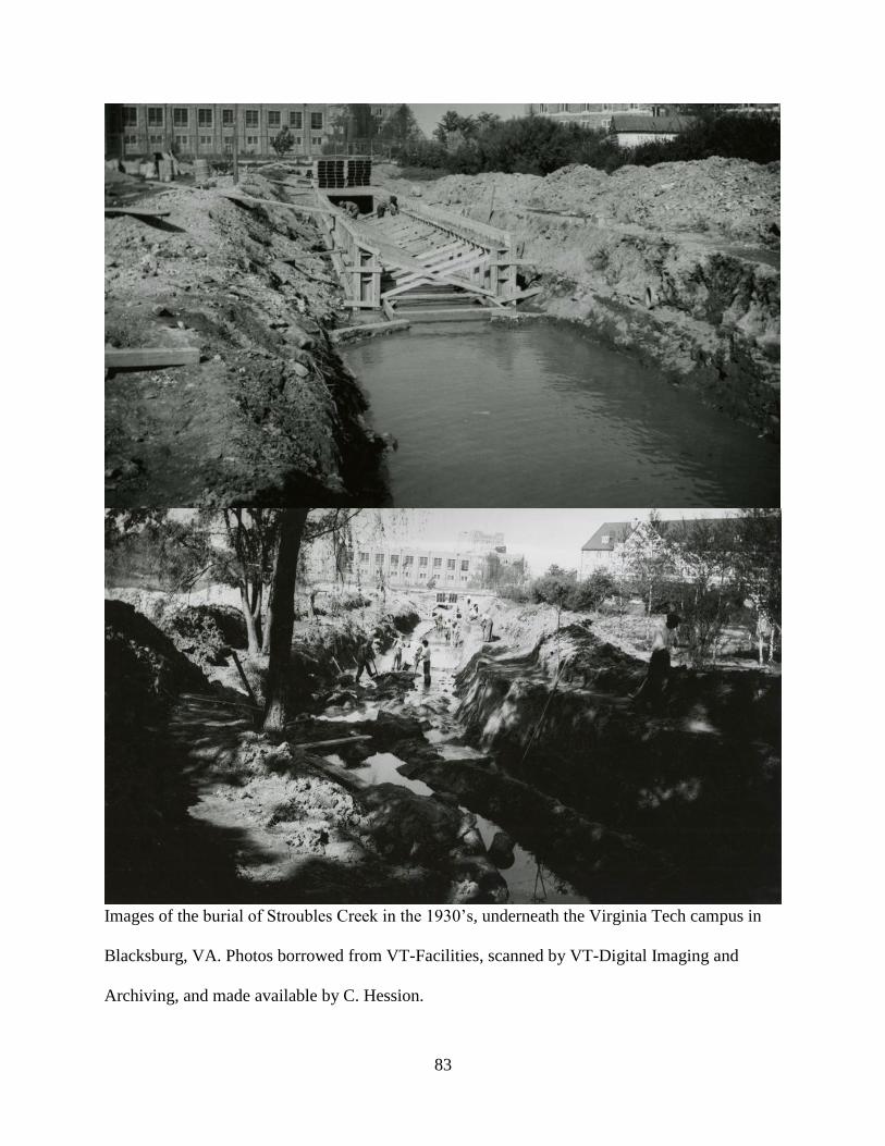
83

Images of the burial of Stroubles Creek in the 1930’s, underneath the Virginia Tech campus in

Blacksburg, VA. Photos borrowed from VT-Facilities, scanned by VT-Digital Imaging and

Archiving, and made available by C. Hession.

84

The move isn’t a recently devised trick. The western world has been moving streams

underground since the Roman Empire. Between then and now, our stream burial technology has

not undergone any revolutions, aside from separating stormwater and raw sewage and using

different pipe materials.

Most people are not aware of the historic streams that have been buried—except for the curious

few who wonder, for instance, why the street in downtown New York City is named “Canal.” In

fact, we’ve buried streams all across the nation—in Los Angeles, D.C, and more. The U.S.’s

Environmental Protection Agency estimates that we’ve buried 98 percent of the streams that

once crossed through Baltimore’s urban core.

Although we’ve buried these streams, we haven’t put them to rest. They are still flowing, and

still take in all the things we shed, spill, drop, and leak into our landscape. As rain runs over

paved streets and sidewalks, it sweeps everything from the urban world directly into the nearest

waterbody. Urban runoff makes its way to these hidden streams.

Unpiped, healthy streams naturally filter much of the water that flows into them. Smaller streams

are mediators of human effluent: receiving the waste discharged from point sources (like

industrial pipes and wastewater treatment plants) and from nonpoint sources (like runoff from

streets and agricultural activities) and using tools like microbes, algae, rocks, and soil to slowly

unload and transform excess nutrients and pollutants. Unwittingly tasked with filtering chemicals

and solutes, natural streams are very important to human health. And when we bury streams, we

rob ourselves of our natural purifiers.

85

Streams typically teem with life: algae, fish, and invertebrates. A stream is home to microbes that

require light, nutrients, and a natural stream bottom. These microorganisms are the power players

that remove those excessive nutrients. But most ghost streams don’t host much life at all. When

we bury a stream underground, we cut it off from light and the stream bottom. Only nutrients

remain, which are funneled downstream, mixing city runoff with fresh water in the nearest river.

“Nutrients” sound good, but they can wreak havoc in downstream waterbodies, polluting

waterways, feeding thick blooms of toxic cyanobacteria, and creating coastal dead zones

Luckily, towns are beginning to acknowledge the importance of these buried streams in an effort

to reduce the terrors of urban runoff. Simply letting locals know a stream exists beneath them,

and that the stream receives everything, untreated, that goes down the drain, encourages people

to keep their waste out of the secret streams.

For example, small frog statues adorn city drains in Blacksburg, Virginia, marking the drains

directly above the local ghost stream. It’s a callback to the Ancient Romans, who marked their

buried streams with shrines to “Cloaca Maxima” or the sewer goddess. Baltimore stencils its

storm drains, and Richmond, Virginia and Dayton, Ohio want to do the same using the work of

local artists. Entry points to waterways are embellished with paintings of fish, octopuses, and

otters encircled by cautionary reminders like “all water drains to the sea” and “only rain should

go down the drain.” Other storm drain murals are decorated with landscape paintings of scenic

86

wildlife, images of kelp with plastic and litter for companions, or paintings of fish where grated

drains act as mouths.

Some places are going further, ripping up pavement, shattering pipes, and hammering away the

concrete to exhume ghost streams. Daylighting, as the procedure is called, opens the streams up

to the sun and restores the adjacent land connection. This begins the process of healing, re-

growing vegetation, and encouraging microbes and algae to come back. It’s great, but unburying

a stream is expensive and requires strong community backing, and community support for

daylighting a stream can’t be mustered if residents aren’t aware of the buried stream itself. Art is

a great first step.

By recognizing ghost streams and getting locals engaged, we can work toward healing the

waterways by limiting the pollutants poured into them, and even eventually unearthing them

from the ground.

87

Chapter Five: General Discussion: Integrating disturbance into our current understanding

of metabolism and stream health

What does a healthy stream look like? Regardless of whether you’re a water quality

practitioner, resource manager, or an ecologist, visions of a healthy stream likely converge on

similar characteristics – geomorphic heterogeneity with a mix of riffles and pools; riparian

connection with thriving plants; access to a moderate amount of sunlight, filtered through a

canopy; relatively clear water with a mix of species swimming about. Historically, stream health

has been monitored and characterized via such structural metrics (Palmer and Febria 2012).

However, as advances in technology (e.g., dissolved oxygen sensors) have made quantifying

functional metrics easier, there has been a shift away from considering what a healthy stream

might look like, to deliberating what a healthy stream does. Does it remove more nutrients? Have

a more stable streambed? Support more productive fisheries? Notably, there has been less

consideration of things like point measurements of oxygen concentration, and more emphasis

placed on biologic oxygen demand and production in the form of stream metabolism (Palmer and

Febria 2012).

Stream metabolism is increasingly being applied as a metric used to quantify stream

health (Young et al. 2008), the response of a stream to a disturbance (e.g., Reisinger et al. 2017;

Chapter 2), and stream recovery following restoration (e.g., Arroita et al. 2019). Some of the

benefits of using metabolism as a bioindicator are well outlined by Young et al. (2008): (1)

metabolism represents the carbon transformations of a whole reach; (2) the ratio of productivity

to respiration can illuminate the balance between energy supply and demand; (3) short time-

scales are needed to estimate metabolism; and (4) metabolism is intimately connected to the

more long-standing health metric of oxygen concentration. Additionally, stream metabolism

88

influences other ecosystem processes; namely, metabolism is related to nutrient uptake (Hall and

Tank 2003), which is critical to the ecosystem service of nitrogen removal (Pataki et al. 2011), as

well as consumer secondary production (Marcarelli et al. 2011).

One notable consideration of applying metabolism as a bioindicator missing from past

discussions is that daily metabolism responds rapidly to disturbances. This is beneficial if trying

to ascertain instantaneous ecosystem response; however, the rapid response of metabolism to

disturbance means that metabolism, and the ecosystem services it is intimately connected to, can

be considerably impacted by flow events – one of the most frequent stream disturbances. With

this in mind, here I discuss: (1) the need to differentiate between stream health and stream

function; (2) the importance of quantifying resistance and resilience of stream metabolism to

frequent flow disturbances; and (3) my recommendations for the future applications of stream

metabolism as a metric of health.

Many ecologists have adopted the mindset, either explicitly or implicitly, that the health

of a stream is related to its likeness to a less altered, reference stream (Boulton 1999, Palmer and

Febria 2012), and this mentality has spilled over into metabolism. One of the most highly cited

papers promoting metabolism as a metric of stream health splits its study sites into two groups

for health characterizations: reference and impacted (Young et al. 2008). Reference sites, and

thus sites with assumed better health, have lower GPP and ER (Young et al. 2008). Although

Young et al. (2008) acknowledge that low metabolism equating to better health is not a universal

rule, this notion can create conflicting ideas of stream health between ecologists and water

quality practitioners by creating a divergence between health and potential function.

Ecological understanding of the relationship between metabolism and health is impaired

by the idea that low GPP and ER represent a healthier system, as this separates the idea of health

89

and function. The function of a stream, and the ability to remove nutrients and also metabolize to

provide the basis of energy for food webs, is often greater in impaired, classically ‘unhealthy’

systems. Forested reference streams are characterized by typically lower rates of GPP and ER.

Therefore, high rates of GPP and ER typically reflect poor stream health; however, streams with

high metabolic rates can have much higher function, and are indicative of either certain types of

catchments (e.g., open canopy grasslands) or of impairment to the catchment, such as the

excessive loading of nutrients from agricultural fields. Additionally, rates of GPP and ER that are

low enough to be categorized as from ‘healthy’ systems according to Young et al.’s criteria have

been recorded in ecosystems ranging from 73-90% developed (Reisinger et al. 2017); we know

these ecosystems are not ‘healthy’ in that they have been severely altered, and yet they are

considered healthy according to this criteria. When assessing the health of the stream, we should

also consider the potential for higher rates of functional metrics.

Low rates of metabolism and likeness to reference streams should not drive our

assessments of metabolism in regard to stream health; instead, we should adopt an understanding

of the relationship between metabolism and stream health that incorporates its potential for

function, and more closely aligns with other functional metrics of stream health, which include,

but are not limited to, pollutant removal rates and nutrient cycling rates (Palmer & Febria 2012).

When ecologists talk about the hidden dangers of excessive nutrient loading and alterations to

stream morphology, we typically warn about the potential for excessive downstream export -

causing the downstream accumulation of biomass, depletion of oxygen, and consequential harm

to biota. Streams with greater function and higher rates of metabolism control nutrient uptake

and retention (Hall and Tank 2003), ultimately alleviating downstream export (Bernhardt et al.

2003). Less function and consequently lower rates of metabolism in a stream loaded with high

90

levels of nutrients would mean that more nutrients are exported downstream. If we adopt a more

ecosystem-service centric metric of metabolism for understanding health, as we should to ensure

that metrics of ecosystem health align between ecologists and water quality practitioners, then

lower rates of metabolism in impaired streams should be considered to be less beneficial for

ecosystem health, as they have less potential for in-stream nutrient removal. However, deeming

higher rates of metabolism and greater function as healthier should be considered in the context

of the ability for nutrient removal, and should be used carefully, as high GPP and ER in some

conditions can result in a build-up of unconsumed primary producers, leading to algal blooms

and/or hypoxia. We do not suggest that the inverse of Young’s criteria is the better route (high

rates of metabolism are healthy and low are unhealthy); rather, we caution against using

metabolic rates as metrics of health overall, without also incorporating a consideration for how

this reflections the functional capacity of the stream.

Elevated flows have disproportionate impacts on stream metabolism and the export of

nutrients (Raymond and Saiers 2010, Inamdar et al. 2015, Bernhardt et al. 2018). Consequently,

we should account for how the transformative potential of metabolism is altered from flow

disturbances through incorporating an understanding of metabolic resistance and resilience

across sites. Resistance is the capacity of a stream process to withstand a disturbance. If

resistance to elevated flows are higher, the large influx of nutrients from the catchment at higher

flows may be mediated to some extent. However, if the resistance is low – as is often seen in

urban, impaired streams with channelized and altered geomorphology – the ability to potentially

offset that nutrient influx is severely hindered. Resilience is the speed at which a process returns

to equilibrium (Carpenter et al. 1992). Metabolic resilience represents how quickly equilibrium

rates of metabolism are resumed following a disturbance. If resilience is low and metabolic

91

recovery is prolonged, the full capacity for metabolism to enhance nutrient uptake is not

achieved, and an opportunity for lessening nutrient export is missed. Understanding the extent

and duration of metabolic impairment following elevated flows – the most frequent stream

disturbance – is critical to our understanding of the utility of metabolism as a component of

stream health in regard to mitigating excessive nutrient loading. Stream health should encompass

multiple functional metrics; if metabolism is to be used and considered in the context of its

ability to mitigate excessive loading from the catchment, then increased resistance and resilience

of GPP and ER are important, and may even play a disproportionate role in lessening nutrient

export over baseflow rates of metabolism.

To begin incorporating the concepts of resistance and resilience into our understanding of

metabolism and stream health, we must first find the best ways to quantify them. Most studies

examine event-scale metabolic responses to flow disturbances, where resistance is calculated via

a percent reduction relative to an antecedent average, and resilience is defined as the rate of

recovery to that antecedent average (e.g., Reisinger et al. 2017; Uehlinger 2000). These studies

typically examine only a handful of flow disturbances at one site, focusing on characterizing

resistance and resilience drivers spatially. Within Chapter 3 of this thesis, I addressed temporal,

within-site variability of GPP and ER resistance and resilience, examining their responses across

15 different flow disturbances. I found that the low resistance/high resilience trends typically

found for urban stream metabolism (Reisinger et al. 2017) were supported within this research,

and both GPP and ER typically recovered within a few days. I also tested which antecedent

conditions or disturbance characteristics drive recovery dynamics of GPP and ER, and found that

the size of the flow disturbance only strongly mattered to ER, and GPP responded similarly

regardless of magnitude.

92

It is possible to quantify metabolic resistance to flow disturbances without looking at

event-scale response. Resistance of processes can be quantified via statistically-derived changes

of slope across discharge in P-Q (process-discharge) relationships, as demonstrated in Chapter 2.

When segmenting P-Q relationships within the second chapter, metabolism did exhibit changes

across low and high discharges. ER and NEP had significant changes across flow, whereas the

slope change for GPP was not significant. The slope change for ER and delayed slope change for

GPP illuminates the potential for divergent responses of ER and GPP at higher flows, and the

potential for different levels of process resistance to flow changes. Additionally, there are other

methods for quantifying metabolic resistance and resilience that were not addressed in this thesis.

Namely, kernel density plots of metabolism that represent the metabolic fingerprint of a site can

be used to examine metabolic resistance or resilience (Bernhardt et al. 2018). The expansion or

contraction of the metabolic fingerprint would enable us to move away from looking at singular

point estimates of metabolism with confounding environmental controls, such as land use or

nutrient concentration, towards instead evaluating the metabolic regime response to a change

(Hall 2016).

In sum, evaluating the impacts disturbances have on stream ecosystem health requires a

clear, contextual definition of health. Low metabolism may be more consistent across forested

reference streams, but lower metabolism in anthropogenically altered systems indicate less

potential for nutrient removal, and consequently more downstream export of excessive nutrients

and pollutants. We should move away from suggesting low rates of metabolism are ‘healthy’.

Additionally, incorporating measurements of resistance and resilience via the novel frameworks

outlined in this thesis would make the understanding of the relationship between stream

metabolism and health more complete. In the face of increasing anthropogenic changes, the

93

effective restoration and conservation of our streams relies on our comprehensive understanding

of the changes that occur to streams following disturbances, and how that may relate to overall

ecosystem health.

94

References

ARROITA, M., A. ELOSEGI, R. O. HALL, S. HAMPTON, M. CHURCH, J. MELACK, AND

M. SCHEUERELL. 2019. Twenty years of daily metabolism show riverine recovery following

sewage abatement. Limnol. Oceanogr 64:77–92.

BERNHARDT, E. S., J. B. HEFFERNAN, N. B. GRIMM, E. H. STANLEY, J. W. HARVEY,

M. ARROITA, A. P. APPLING, M. J. COHEN, W. H. MCDOWELL, R. O. HALL, J. S. READ,

B. J. ROBERTS, E. G. STETS, AND C. B. YACKULIC. 2018. The metabolic regimes of

flowing waters.

BERNHARDT, E. S., G. E. LIKENS, D. C. BUSO, AND C. T. DRISCOLL. 2003. In-stream

uptake dampens effects of major forest disturbance on watershed nitrogen export. Proceedings of

the National Academy of Sciences of the United States of America 100:10304–8.

BOULTON, A. J. 1999. An overview of river health assessment: philosophies, practice,

problems and prognosis. Freshwater Biology 41:469–479.

CARPENTER, S. R., C. E. KRAFT, R. WRIGHT, X. HE, P. A. SORANNO, AND J. R.

HODGSON. 1992. Resilience and resistance of a lake phosphorus cycle before and after food

web manipulation. The American naturalist 140:781–98.

HALL, R. 2016. Metabolism of Streams and Rivers: Estimation, Controls, and Application.

Pages 151–173 in J. Jones and E. Stanley (editors). Stream Ecosystems in a Changing

Environment. Elsevier.

HALL, R. J. O., AND J. L. TANK. 2003. Ecosystem metabolism controls nitrogen uptake in

streams in Grand Teton National Park, Wyoming. Limnology and Oceanography 48:1120–1128.

INAMDAR, S., G. DHILLON, S. SINGH, T. PARR, AND Z. QIN. 2015. Particulate nitrogen

exports in stream runoff exceed dissolved nitrogen forms during large tropical storms in a

temperate, headwater, forested watershed. Journal of Geophysical Research: Biogeosciences

120:1548–1566.

MARCARELLI, A. M., C. V. BAXTER, M. M. MINEAU, AND R. O. HALL. 2011. Quantity

and quality: unifying food web and ecosystem perspectives on the role of resource subsidies in

freshwaters. Ecology 92:1215–1225.

PALMER, M., AND C. FEBRIA. 2012. The Heartbeat of Ecosystems. Science 336:1393–1394.

PATAKI, D. E., M. M. CARREIRO, J. CHERRIER, N. E. GRULKE, V. JENNINGS, S.

PINCETL, R. V POUYAT, T. H. WHITLOW, AND W. C. ZIPPERER. 2011. Coupling

biogeochemical cycles in urban environments: ecosystem services, green solutions, and

misconceptions. Frontiers in Ecology and the Environment 9:27–36.

RAYMOND, P. A., AND J. E. SAIERS. 2010. Event controlled DOC export from forested

watersheds. Biogeochemistry 100:197–209.

REISINGER, A. J., E. J. ROSI, H. A. BECHTOLD, T. R. DOODY, S. S. KAUSHAL, AND P.

M. GROFFMAN. 2017. Recovery and resilience of urban stream metabolism following

Superstorm Sandy and other floods. Ecosphere 8.

95

UEHLINGER, U. 2000. Resistance and resilience of ecosystem metabolism in a flood-prone

river system. Freshwater Biology 45:319–332.

YOUNG, R. G., C. D. MATTHAEI, AND C. R. TOWNSEND. 2008. Organic matter breakdown

and ecosystem metabolism: functional indicators for assessing river ecosystem health. Journal of

the North American Benthological Society 27:605–625.

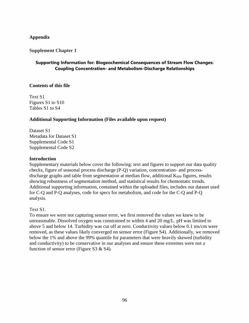
96

Appendix

Supplement Chapter 1

Supporting Information for: Biogeochemical Consequences of Stream Flow Changes:

Coupling Concentration- and Metabolism-Discharge Relationships

Contents of this file

Text S1

Figures S1 to S10

Tables S1 to S4

Additional Supporting Information (Files available upon request)

Dataset S1

Metadata for Dataset S1

Supplemental Code S1

Supplemental Code S2

Introduction

Supplementary materials below cover the following: text and figures to support our data quality

checks, figure of seasonal process discharge (P-Q) variation, concentration- and process-

discharge graphs and table from segmentation at median flow, additional K600 figures, results

showing robustness of segmentation method, and statistical results for chemostatic trends.

Additional supporting information, contained within the uploaded files, includes our dataset used

for C-Q and P-Q analyses, code for specs for metabolism, and code for the C-Q and P-Q

analysis.

Text S1.

To ensure we were not capturing sensor error, we first removed the values we knew to be

unreasonable. Dissolved oxygen was constrained to within 4 and 20 mg/L. pH was limited to

above 5 and below 14. Turbidity was cut off at zero. Conductivity values below 0.1 ms/cm were

removed, as these values likely converged on sensor error (Figure S4). Additionally, we removed

below the 1% and above the 99% quantile for parameters that were heavily skewed (turbidity

and conductivity) to be conservative in our analyses and ensure these extremes were not a

function of sensor error (Figure S3 & S4).

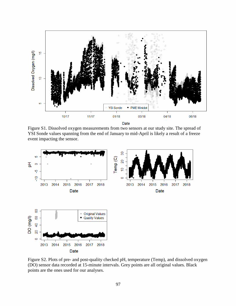
97

Figure S1. Dissolved oxygen measurements from two sensors at our study site. The spread of

YSI Sonde values spanning from the end of January to mid-April is likely a result of a freeze

event impacting the sensor.

Figure S2. Plots of pre- and post-quality checked pH, temperature (Temp), and dissolved oxygen

(DO) sensor data recorded at 15-minute intervals. Grey points are all original values. Black

points are the ones used for our analyses.

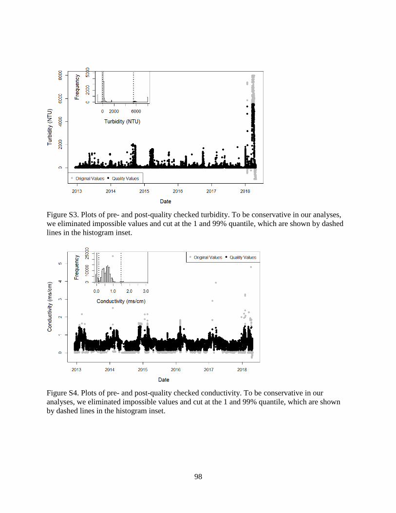
98

Figure S3. Plots of pre- and post-quality checked turbidity. To be conservative in our analyses,

we eliminated impossible values and cut at the 1 and 99% quantile, which are shown by dashed

lines in the histogram inset.

Figure S4. Plots of pre- and post-quality checked conductivity. To be conservative in our

analyses, we eliminated impossible values and cut at the 1 and 99% quantile, which are shown

by dashed lines in the histogram inset.

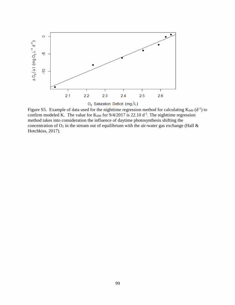
99

Figure S5. Example of data used for the nighttime regression method for calculating K600 (d

-1) to

confirm modeled K. The value for K600 for 9/4/2017 is 22.10 d-1. The nighttime regression

method takes into consideration the influence of daytime photosynthesis shifting the

concentration of O2 in the stream out of equilibrium with the air-water gas exchange (Hall &

Hotchkiss, 2017).

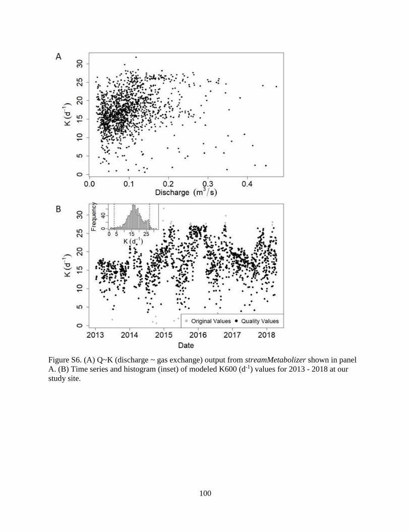
100

Figure S6. (A) Q~K (discharge ~ gas exchange) output from streamMetabolizer shown in panel

A. (B) Time series and histogram (inset) of modeled K600 (d-1) values for 2013 - 2018 at our

study site.

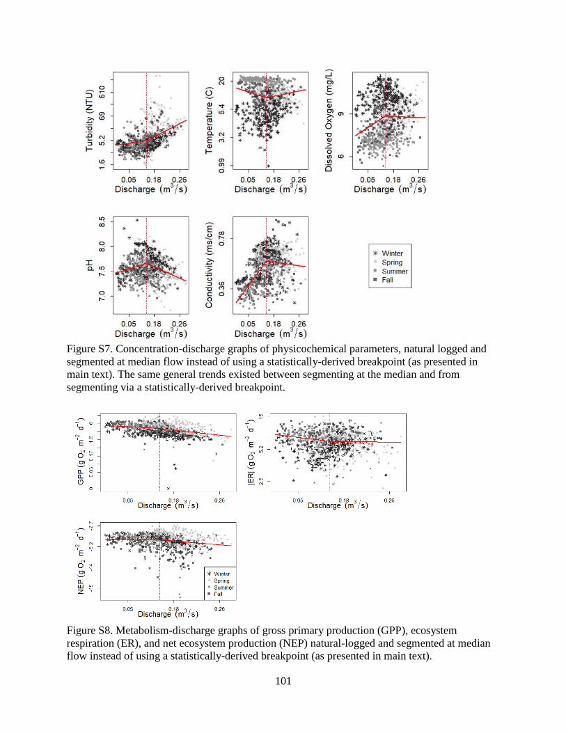
101

Figure S7. Concentration-discharge graphs of physicochemical parameters, natural logged and

segmented at median flow instead of using a statistically-derived breakpoint (as presented in

main text). The same general trends existed between segmenting at the median and from

segmenting via a statistically-derived breakpoint.

Figure S8. Metabolism-discharge graphs of gross primary production (GPP), ecosystem

respiration (ER), and net ecosystem production (NEP) natural-logged and segmented at median

flow instead of using a statistically-derived breakpoint (as presented in main text).

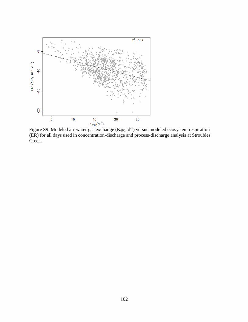
102

Figure S9. Modeled air-water gas exchange (K600, d

-1) versus modeled ecosystem respiration

(ER) for all days used in concentration-discharge and process-discharge analysis at Stroubles

Creek.

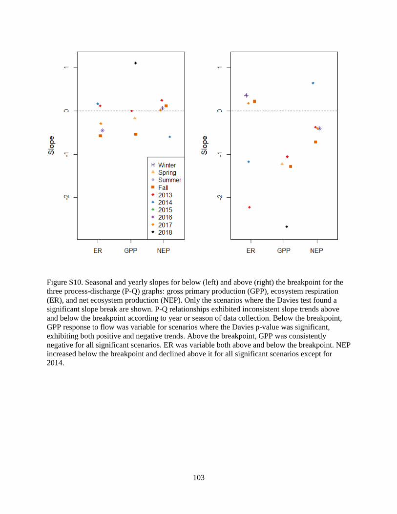
103

Figure S10. Seasonal and yearly slopes for below (left) and above (right) the breakpoint for the

three process-discharge (P-Q) graphs: gross primary production (GPP), ecosystem respiration

(ER), and net ecosystem production (NEP). Only the scenarios where the Davies test found a

significant slope break are shown. P-Q relationships exhibited inconsistent slope trends above

and below the breakpoint according to year or season of data collection. Below the breakpoint,

GPP response to flow was variable for scenarios where the Davies p-value was significant,

exhibiting both positive and negative trends. Above the breakpoint, GPP was consistently

negative for all significant scenarios. ER was variable both above and below the breakpoint. NEP

increased below the breakpoint and declined above it for all significant scenarios except for

2014.

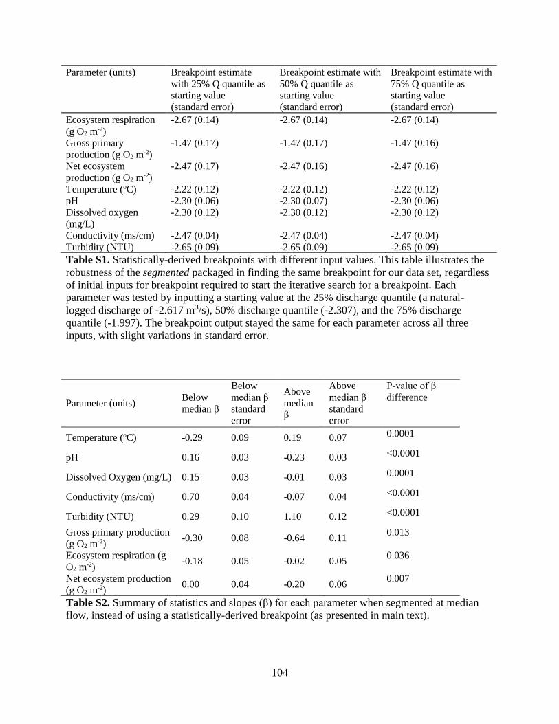
104

Parameter (units) Breakpoint estimate

with 25% Q quantile as

starting value

(standard error)

Breakpoint estimate with

50% Q quantile as

starting value

(standard error)

Breakpoint estimate with

75% Q quantile as

starting value

(standard error)

Ecosystem respiration

(g O2 m-2)

-2.67 (0.14) -2.67 (0.14) -2.67 (0.14)

Gross primary

production (g O2 m-2)

-1.47 (0.17) -1.47 (0.17) -1.47 (0.16)

Net ecosystem

production (g O2 m-2)

-2.47 (0.17) -2.47 (0.16) -2.47 (0.16)

Temperature (oC) -2.22 (0.12) -2.22 (0.12) -2.22 (0.12)

pH -2.30 (0.06) -2.30 (0.07) -2.30 (0.06)

Dissolved oxygen

(mg/L)

-2.30 (0.12) -2.30 (0.12) -2.30 (0.12)

Conductivity (ms/cm) -2.47 (0.04) -2.47 (0.04) -2.47 (0.04)

Turbidity (NTU) -2.65 (0.09) -2.65 (0.09) -2.65 (0.09)

Table S1. Statistically-derived breakpoints with different input values. This table illustrates the

robustness of the segmented packaged in finding the same breakpoint for our data set, regardless

of initial inputs for breakpoint required to start the iterative search for a breakpoint. Each

parameter was tested by inputting a starting value at the 25% discharge quantile (a natural-

logged discharge of -2.617 m3/s), 50% discharge quantile (-2.307), and the 75% discharge

quantile (-1.997). The breakpoint output stayed the same for each parameter across all three

inputs, with slight variations in standard error.

Parameter (units) Below

median β

Below

median β

standard

error

Above

median

β

Above

median β

standard

error

P-value of β

difference

Temperature (oC) -0.29 0.09 0.19 0.07 0.0001

pH 0.16 0.03 -0.23 0.03 <0.0001

Dissolved Oxygen (mg/L) 0.15 0.03 -0.01 0.03 0.0001

Conductivity (ms/cm) 0.70 0.04 -0.07 0.04 <0.0001

Turbidity (NTU) 0.29 0.10 1.10 0.12 <0.0001

Gross primary production

(g O2 m-2) -0.30 0.08 -0.64 0.11

0.013

Ecosystem respiration (g

O2 m-2) -0.18 0.05 -0.02 0.05

0.036

Net ecosystem production

(g O2 m-2) 0.00 0.04 -0.20 0.06

0.007

Table S2. Summary of statistics and slopes (β) for each parameter when segmented at median

flow, instead of using a statistically-derived breakpoint (as presented in main text).

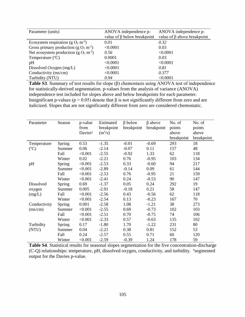
105

Parameter (units) ANOVA independence p-

value of β below breakpoint

ANOVA independence p-

value of β above breakpoint

Ecosystem respiration (g O2 m-2) 0.01 0.32

Gross primary production (g O2 m-2) <0.0001 0.03

Net ecosystem production (g O2 m-2) 0.56 <0.0001

Temperature (oC) 0.0001 0.03

pH <0.0001 <0.0001

Dissolved Oxygen (mg/L) <0.0001 0.81

Conductivity (ms/cm) <0.0001 0.377

Turbidity (NTU) 0.94 <0.0001

Table S3. Summary of test results for slope (β) chemostasis using ANOVA test of independence

for statistically-derived segmentation. p-values from the analysis of variance (ANOVA)

independence test included for slopes above and below breakpoints for each parameter.

Insignificant p-values (p > 0.05) denote that β is not significantly different from zero and are

italicized. Slopes that are not significantly different from zero are considered chemostatic.

Parameter Season p-value

from

Daviesa

Estimated

breakpoint

(m3/s)

β below

breakpoint

β above

breakpoint

No. of

points

above

breakpoint

No. of

points

above

breakpoint

Temperature

(oC)

Spring 0.53 -1.35 -0.01 -0.69 293 18

Summer 0.06 -2.14 -0.07 0.11 157 48

Fall <0.001 -2.55 -0.92 1.33 62 118

Winter 0.02 -2.21 0.76 -0.95 103 134

pH

Spring <0.001 -2.53 0.33 -0.60 94 217

Summer <0.001 -2.89 -0.14 0.09 61 144

Fall <0.001 -2.53 0.76 -0.95 21 159

Winter <0.001 -2.41 0.24 -0.53 90 147

Dissolved

oxygen

(mg/L)

Spring 0.69 -1.37 0.05 0.24 292 19

Summer 0.005 -2.91 -0.18 0.21 58 147

Fall <0.001 -2.56 0.43 -0.56 62 118

Winter <0.001 -2.54 0.13 -0.23 167 70

Conductivity

(ms/cm)

Spring 0.001 -2.58 1.08 -1.21 38 273

Summer <0.001 -2.55 0.69 -0.73 102 103

Fall <0.001 -2.51 0.70 -0.75 74 106

Winter <0.001 -2.33 0.57 -0.63 135 102

Turbidity

(NTU)

Spring 0.17 -1.80 1.70 -1.22 231 80

Summer 0.04 -2.21 0.38 0.81 152 53

Fall 0.24 -2.57 0.55 0.71 60 120

Winter <0.001 -2.59 -0.39 1.24 178 59

Table S4. Statistical results for seasonal slopes segmentation for the five concentration-discharge

(C-Q) relationships: temperature, pH, dissolved oxygen, conductivity, and turbidity. asegmented

output for the Davies p-value.

106

Supplement Chapter 2

Supporting Information for: Resistance and resilience of stream metabolism to isolated

flow events of various magnitudes

Contents of this file

Figures S1, S2

Figure S3 – S17: Hydrographs and metabolism time series for each isolated flow event analyzed

Figures S18, S19

Table S1

Additional Supporting Information (Files available upon request)

Dataset S1

Metadata for Dataset S1

Supplemental Code S1

Figure S1. Dissolved oxygen measurements from the two sensors – YSI Sonde and PME

Minidot - at our study site. The spread of YSI Sonde values spanning from the end of January to

mid-April was likely a result of a freeze event that impacted the sensor.

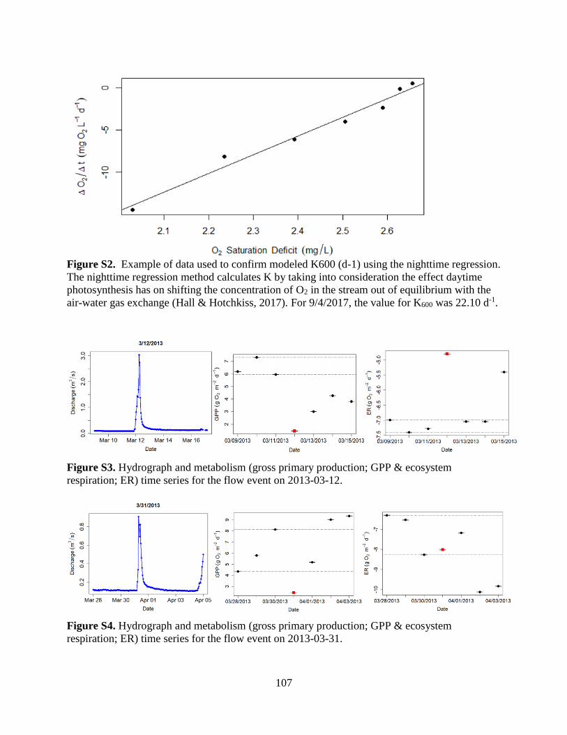
107

Figure S2. Example of data used to confirm modeled K600 (d-1) using the nighttime regression.

The nighttime regression method calculates K by taking into consideration the effect daytime

photosynthesis has on shifting the concentration of O2 in the stream out of equilibrium with the

air-water gas exchange (Hall & Hotchkiss, 2017). For 9/4/2017, the value for K600 was 22.10 d-1.

Figure S3. Hydrograph and metabolism (gross primary production; GPP & ecosystem

respiration; ER) time series for the flow event on 2013-03-12.

Figure S4. Hydrograph and metabolism (gross primary production; GPP & ecosystem

respiration; ER) time series for the flow event on 2013-03-31.

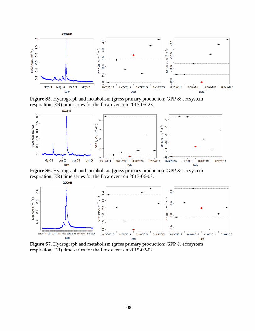
108

Figure S5. Hydrograph and metabolism (gross primary production; GPP & ecosystem

respiration; ER) time series for the flow event on 2013-05-23.

Figure S6. Hydrograph and metabolism (gross primary production; GPP & ecosystem

respiration; ER) time series for the flow event on 2013-06-02.

Figure S7. Hydrograph and metabolism (gross primary production; GPP & ecosystem

respiration; ER) time series for the flow event on 2015-02-02.

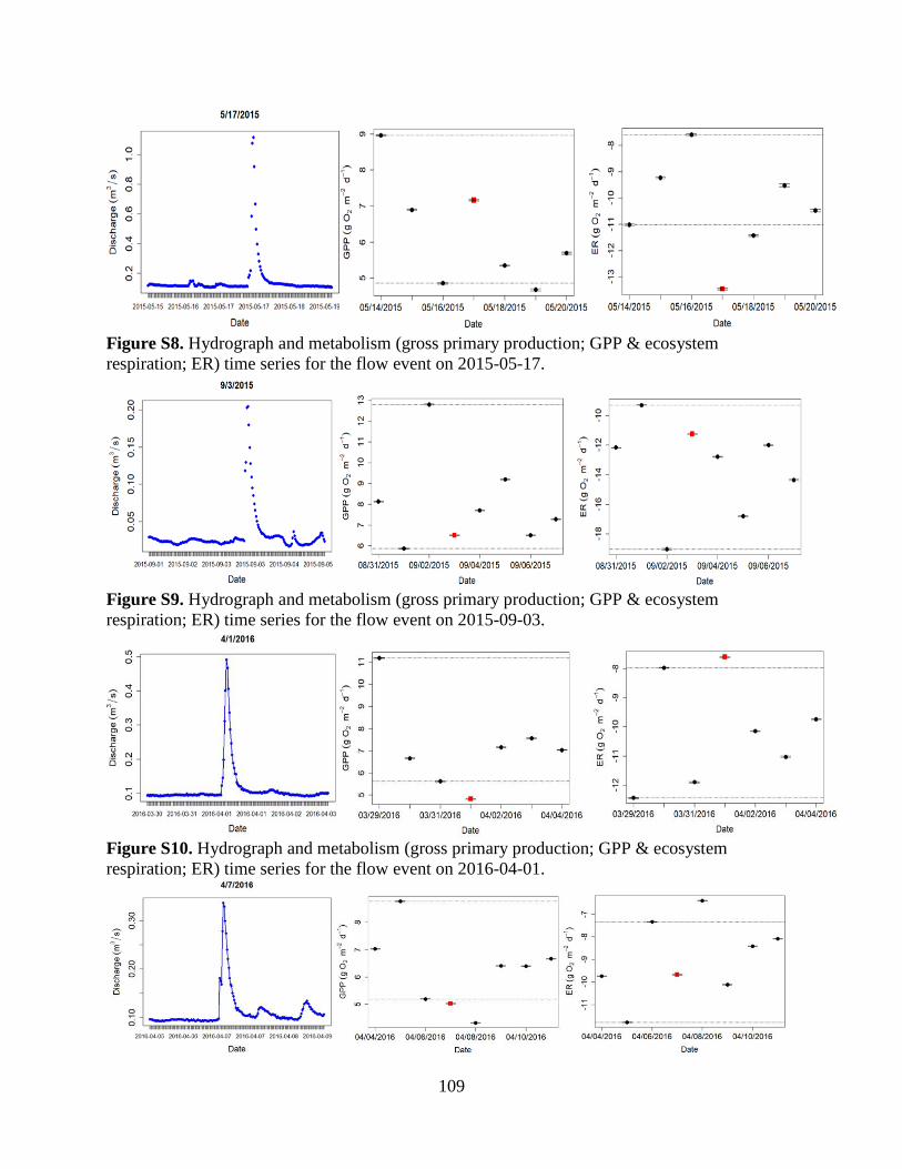
109

Figure S8. Hydrograph and metabolism (gross primary production; GPP & ecosystem

respiration; ER) time series for the flow event on 2015-05-17.

Figure S9. Hydrograph and metabolism (gross primary production; GPP & ecosystem

respiration; ER) time series for the flow event on 2015-09-03.

Figure S10. Hydrograph and metabolism (gross primary production; GPP & ecosystem

respiration; ER) time series for the flow event on 2016-04-01.

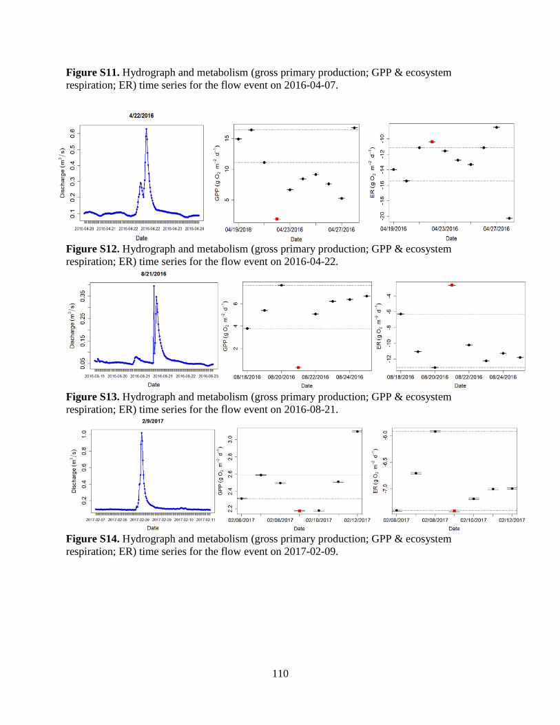
110

Figure S11. Hydrograph and metabolism (gross primary production; GPP & ecosystem

respiration; ER) time series for the flow event on 2016-04-07.

Figure S12. Hydrograph and metabolism (gross primary production; GPP & ecosystem

respiration; ER) time series for the flow event on 2016-04-22.

Figure S13. Hydrograph and metabolism (gross primary production; GPP & ecosystem

respiration; ER) time series for the flow event on 2016-08-21.

Figure S14. Hydrograph and metabolism (gross primary production; GPP & ecosystem

respiration; ER) time series for the flow event on 2017-02-09.

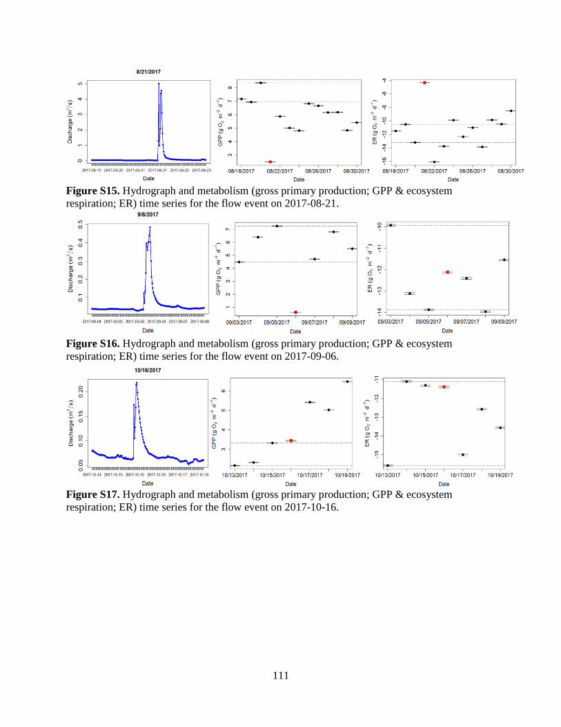
111

Figure S15. Hydrograph and metabolism (gross primary production; GPP & ecosystem

respiration; ER) time series for the flow event on 2017-08-21.

Figure S16. Hydrograph and metabolism (gross primary production; GPP & ecosystem

respiration; ER) time series for the flow event on 2017-09-06.

Figure S17. Hydrograph and metabolism (gross primary production; GPP & ecosystem

respiration; ER) time series for the flow event on 2017-10-16.

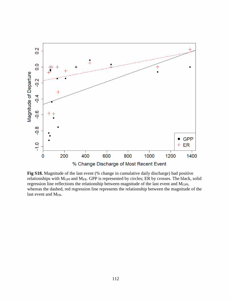
112

Fig S18. Magnitude of the last event (% change in cumulative daily discharge) had positive

relationships with MGPP and MER. GPP is represented by circles; ER by crosses. The black, solid

regression line reflections the relationship between magnitude of the last event and MGPP,

whereas the dashed, red regression line represents the relationship between the magnitude of the

last event and MER.

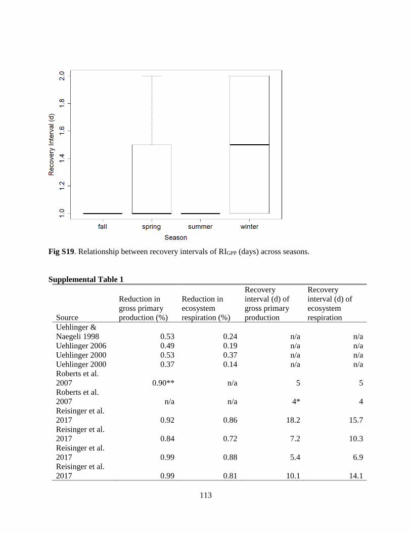
113

Fig S19. Relationship between recovery intervals of RIGPP (days) across seasons.

Supplemental Table 1

Source

Reduction in

gross primary

production (%)

Reduction in

ecosystem

respiration (%)

Recovery

interval (d) of

gross primary

production

Recovery

interval (d) of

ecosystem

respiration

Uehlinger &

Naegeli 1998 0.53 0.24 n/a n/a

Uehlinger 2006 0.49 0.19 n/a n/a

Uehlinger 2000 0.53 0.37 n/a n/a

Uehlinger 2000 0.37 0.14 n/a n/a

Roberts et al.

2007 0.90** n/a 5 5

Roberts et al.

2007 n/a n/a 4* 4

Reisinger et al.

2017 0.92 0.86 18.2 15.7

Reisinger et al.

2017 0.84 0.72 7.2 10.3

Reisinger et al.

2017 0.99 0.88 5.4 6.9

Reisinger et al.

2017 0.99 0.81 10.1 14.1

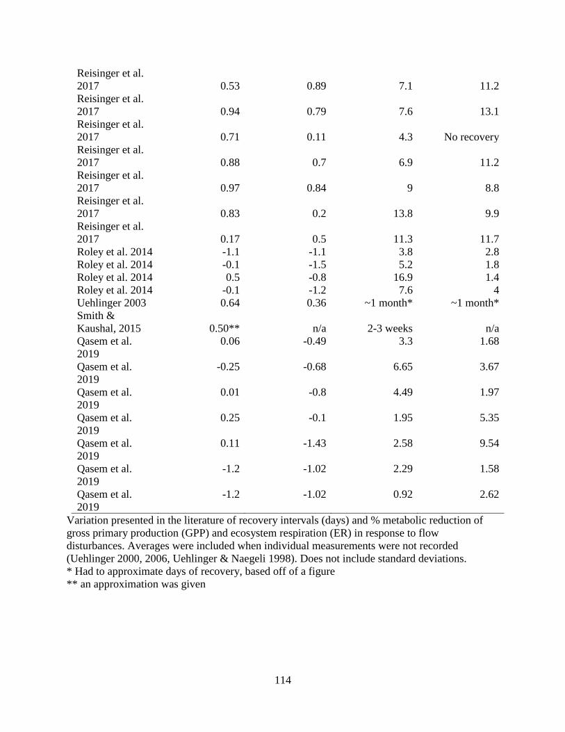
114

Reisinger et al.

2017 0.53 0.89 7.1 11.2

Reisinger et al.

2017 0.94 0.79 7.6 13.1

Reisinger et al.

2017 0.71 0.11 4.3 No recovery

Reisinger et al.

2017 0.88 0.7 6.9 11.2

Reisinger et al.

2017 0.97 0.84 9 8.8

Reisinger et al.

2017 0.83 0.2 13.8 9.9

Reisinger et al.

2017 0.17 0.5 11.3 11.7

Roley et al. 2014 -1.1 -1.1 3.8 2.8

Roley et al. 2014 -0.1 -1.5 5.2 1.8

Roley et al. 2014 0.5 -0.8 16.9 1.4

Roley et al. 2014 -0.1 -1.2 7.6 4

Uehlinger 2003 0.64 0.36 ~1 month* ~1 month*

Smith &

Kaushal, 2015 0.50** n/a 2-3 weeks n/a

Qasem et al.

2019

0.06 -0.49 3.3 1.68

Qasem et al.

2019

-0.25 -0.68 6.65 3.67

Qasem et al.

2019

0.01 -0.8 4.49 1.97

Qasem et al.

2019

0.25 -0.1 1.95 5.35

Qasem et al.

2019

0.11 -1.43 2.58 9.54

Qasem et al.

2019

-1.2 -1.02 2.29 1.58

Qasem et al.

2019

-1.2 -1.02 0.92 2.62

Variation presented in the literature of recovery intervals (days) and % metabolic reduction of

gross primary production (GPP) and ecosystem respiration (ER) in response to flow

disturbances. Averages were included when individual measurements were not recorded

(Uehlinger 2000, 2006, Uehlinger & Naegeli 1998). Does not include standard deviations.

* Had to approximate days of recovery, based off of a figure

** an approximation was given