The Finite Element Method for the Analysis of Non …webarchiv.ethz.ch/ibk/emeritus/fa/education/FE_II/Lecture_1.pdf · Swiss Federal Institute of Technology Page 1 Method of Finite

Swiss Federal Institute of Technology Page 1

Method of Finite Elements II

The Finite Element Method for the Analysis of Non-Linear and Dynamic Systems

Prof. Dr. Michael Havbro Faber

Swiss Federal Institute of TechnologyETH Zurich, Switzerland



Contents of Today's Lecture

• Motivation, overview and organization of the course

• Introduction to non-linear analysis

• Formulation of the continuum mechanics incremental equations of motion



Motivation, overview and organization of the course

• Motivation

In FEM 1 we learned about the steady state analysis of linear systems

however,

the systems we are dealing with in structural engineering are generally not steady state and also not linear

We must be able to assess the need for a particular type of analysis and we must be able to perform it




• Motivation

What kind of problems are not steady state and linear?

E.g. when the:

material behaves non-linearly

deformations become big (p-Δ effects)

loads vary fast compared to the eigenfrequencies of the structure

General feature: Response becomes load path dependent




• Motivation

What is the “added value” of being able to assess the non-linear non-steady state response of structures ?

E.g. assessing the:

- structural response of structures to extreme events (rock-fall, earthquake, hurricanes)

- performance (failures and deformations) of soils

- verifying simple models




• Collapse Analysis of the World Trade Center




• Collapse Analysis of the World Trade Center




• Analysis of ultimate collapse capacity of jacket structure




• Analysis of ultimate collapse capacity of jacket structure




• Analysis of soil performance




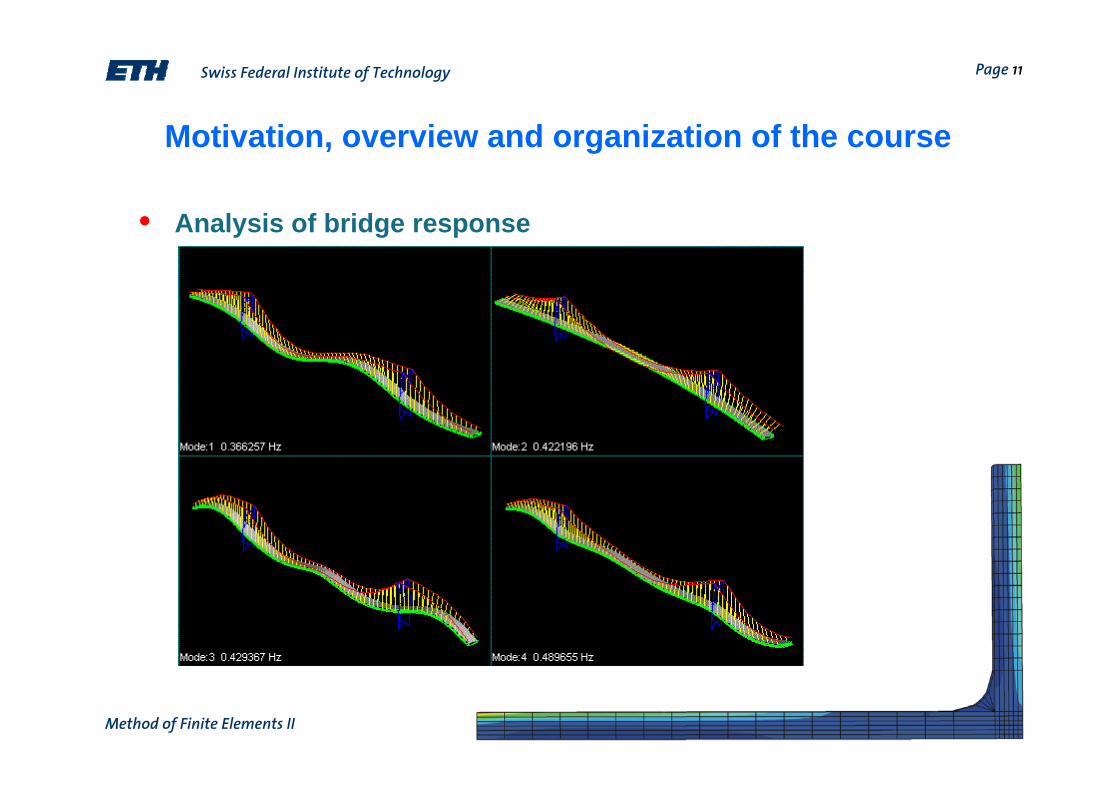
• Analysis of bridge response




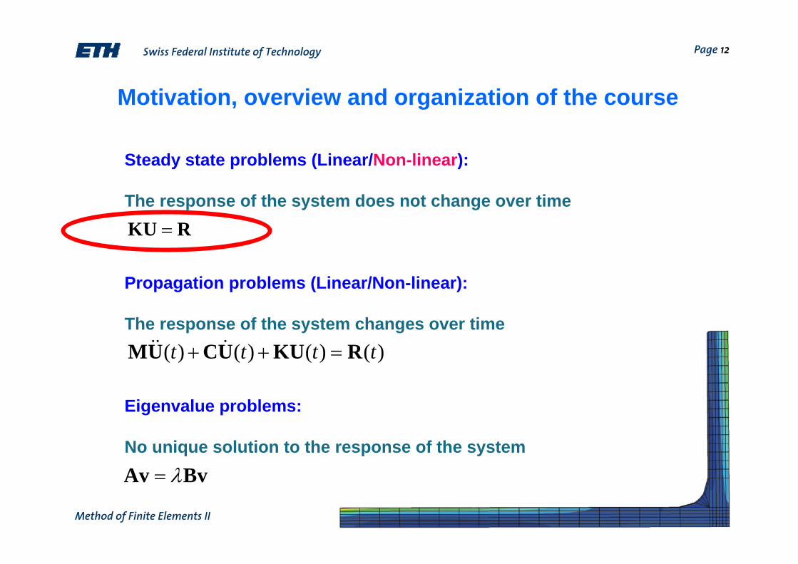
Steady state problems (Linear/Non-linear):

The response of the system does not change over time

Propagation problems (Linear/Non-linear):

The response of the system changes over time

Eigenvalue problems:

No unique solution to the response of the system

=KU R

( ) ( ) ( ) ( )t t t t+ + =MU CU KU R

λ=Av Bv




• Organization

The lectures will be given by:

M. H. Faber

Exercises will be organized/attended by:

Jianjun Qin

By appointment, HIL E13.1.




• Organization

PowerPoint files with the presentations will be uploaded on our homepage one day in advance of the lectures

http://www.ibk.ethz.ch/fa/education/FE_II

The lecture as such will follow the book:

"Finite Element Procedures" by K.J. Bathe, Prentice Hall, 1996




• Overview



• Overview





• Overview



Introduction to non-linear analysis

• Previously we considered the solution of the following linear and static problem:

for these problems we have the convenient property of linearity, i.e:

=KU R

, 1

, 1

λ λ

λ λ∗

= =

⇓

= ≠

KU R

U U

If this is not the case we are dealing with a non-linear problem!



Introduction to non-linear analysis

• Previously we considered the solution of the following linear and static problem:

we assumed:

small displacements when developing the stiffness matrix K and the load vector R, because we performed all integrations over the original element volume

that the B matrix is constant independent of element displacements

the stress-strain matrix C is constant

boundary constraints are constant

=KU R



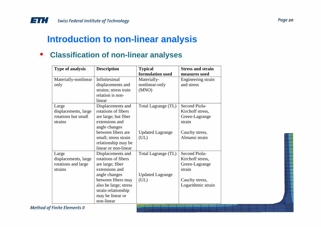
Introduction to non-linear analysis• Classification of non-linear analyses

Type of analysis Description Typical formulation used

Stress and strain measures used

Materially-nonlinear only

Infinitesimal displacements and strains; stress train relation is non-linear

Materially-nonlinear-only (MNO)

Engineering strain and stress

Large displacements, large rotations but small strains

Displacements and rotations of fibers are large; but fiber extensions and angle changes between fibers are small; stress strain relationship may be linear or non-linear

Total Lagrange (TL) Updated Lagrange (UL)

Second Piola-Kirchoff stress, Green-Lagrange strain Cauchy stress, Almansi strain

Large displacements, large rotations and large strains

Displacements and rotations of fibers are large; fiber extensions and angle changes between fibers may also be large; stress strain relationship may be linear or non-linear

Total Lagrange (TL) Updated Lagrange (UL)

Second Piola-Kirchoff stress, Green-Lagrange strain Cauchy stress, Logarithmic strain




Δ

2P

2P ε

σ

1

E

0.04ε <

Linear elastic (infinitesimal displacements)

L

L

//

P AE

L

σε σ

ε

==

Δ =




Δ

2P

2P ε

σ

Materially nonlinear only (infinitesimal displacements, but nonlinear stress-strain relation)

L

L

/

0.04

Y Y

T

P A

E E

σσ σ σε

ε

=−

= +

<

/P A

1

E1 TEYσ




Large displacements and large rotations but small strains (linear or nonlinear material behavior)

x

y

L

x′

y′

L

′Δ

ε′

0.04L

εε

′ <′ ′Δ =




Large displacements, large rotations and large strains (linear or nonlinear material behavior)




Δ

2P

Chang in boundary conditions

2P



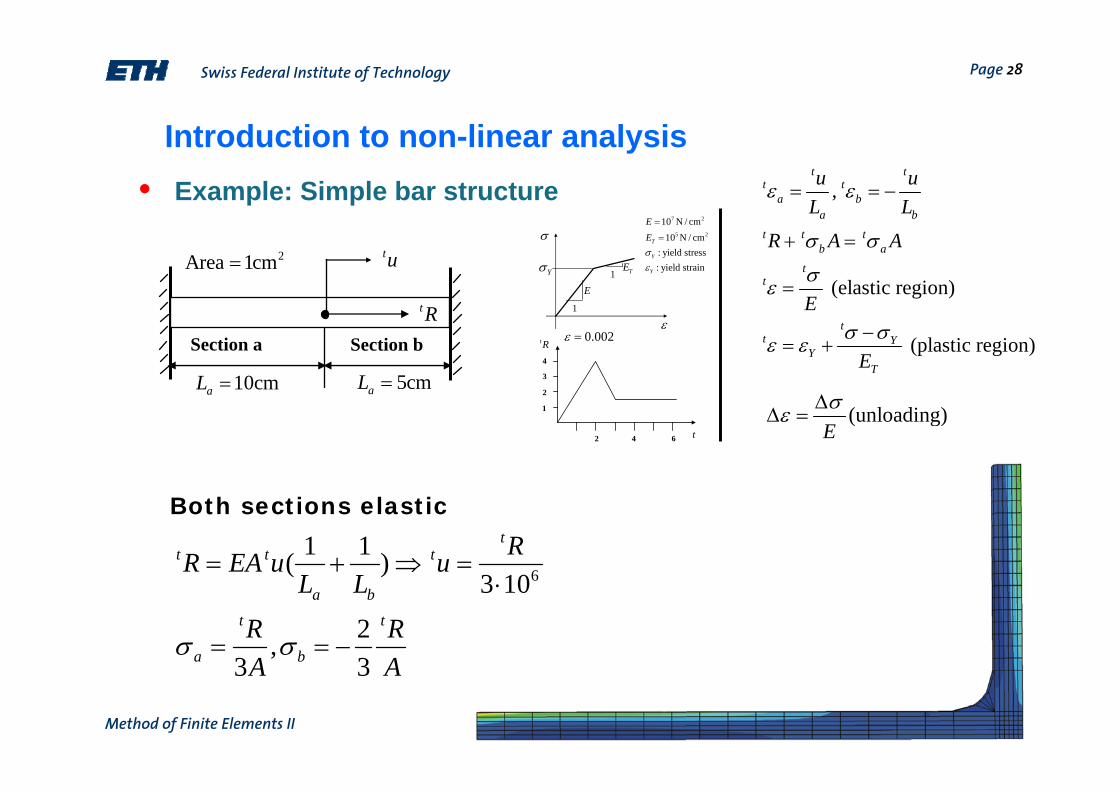
Introduction to non-linear analysis• Example: Simple bar structure

Section a Section b

10cmaL = 5cmbL =

tR

tu2Area 1cm=

ε

σ

1

E1 TEYσ

0.002Yε =

7 2

5 2

10 N / cm10 N / cm

: yield stress: yield strain

T

Y

Y

EEσε

=

=

1

2

3

4

2 4 6

tR

t




Section a Section b

10cmaL = 5cmbL =

tR

tu2Area 1cm=

,

(elastic region)

(plastic region)

t tt t

a ba b

t t tb a

tt

tt Y

YT

u uL L

R A A

E

E

ε ε

σ σ

σε

σ σε ε

= = −

+ =

=

−= +

ε

σ

1

E1 TEYσ

0.002ε =

7 2

5 2

10 N / cm10 N / cm


T

Y

Y

EEσε

=

=

1

2

3

4

2 4 6

tR

t

(unloading)Eσε Δ

Δ =




Section a Section b

10cmaL = 5cmaL =

tR

tu2Area 1cm=

,

(elastic region)

(plastic region)

t tt t

a ba b

t t tb a

tt

tt Y

YT

u uL L

R A A

E

E

ε ε

σ σ

σε

σ σε ε

= = −

+ =

=

−= +

(unloading)Eσε Δ

Δ =

ε

σ

1

E1 TEYσ

0.002ε =

7 2

5 2

10 N / cm10 N / cm


T

Y

Y

EEσε

=

=

1

2

3

4

2 4 6

tR

t

6

1 1( )3 10

2,3 3

tt t t

a b

t t

a b

RR EA u uL L

R RA A

σ σ

= + ⇒ =⋅

= = −

Both sections elastic




Section a Section b

10cmaL = 5cmbL =

tR

tu2Area 1cm=

,

(elastic region)

(plastic region)

t tt t

a ba b

t t tb a

tt

tt Y

YT

u uL L

R A A

E

E

ε ε

σ σ

σε

σ σε ε

= = −

+ =

=

−= +

(unloading)Eσε Δ

Δ =

ε

σ

1

E1 TEYσ

0.002ε =

7 2

5 2

10 N / cm10 N / cm


T

Y

Y

EEσε

=

=

1

2

3

4

2 4 6

tR

t

3section b will be plastic when 2

tYR Aσ

∗

=

Section a is elastic while section b is plastic

, ( )t t

a b T Y Ya b

u uE EL L

σ σ ε σ= = − − −

26

/ 1.9412 10/ / 1.02 10

ttt T

T Y Ya b

t tt T Y Y

a b

E A uEA uR E A AL L

R A E RuE L E L

ε σ

ε σ −

= + − + ⇒

+ −= = − ⋅

+ ⋅

tR

tu0.1 0.2

4

321



Introduction to non-linear analysis• What did we learn from the example?

The basic problem in general nonlinear analysis is to find a state of equilibrium between externally applied loads and element nodal forces

( )

( ) ( ) ( )

0

t m

t t

t t t tB S C

t tI

t t m T t m t m

m V

dVτ

− =

= + +

=

=∑ ∫

R F

R R R R

F R

F B

We must achieve equilibrium for all time steps when incrementing the loading

Very general approach

includes implicitly also dynamicanalysis!



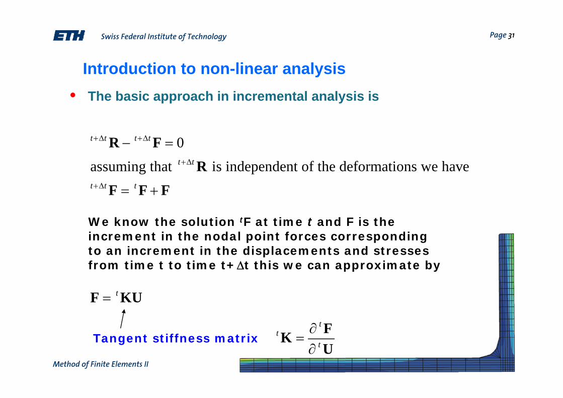
Introduction to non-linear analysis• The basic approach in incremental analysis is

0assuming that is independent of the deformations we have

t t t t

t t

t t t

+Δ +Δ

+Δ

+Δ

− =

= +

R FR

F F F

We know the solution tF at time t and F is the increment in the nodal point forces corresponding to an increment in the displacements and stresses from time t to time t+Δt this we can approximate by

t=F KU

Tangent stiffness matrixt

tt

∂=∂

FKU




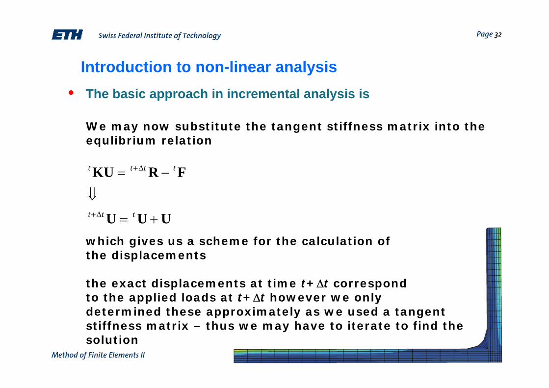
We may now substitute the tangent stiffness matrix into the equlibrium relation

t t t t

t t t

+Δ

+Δ

= −

⇓

= +

KU R F

U U Uwhich gives us a scheme for the calculation of the displacements

the exact displacements at time t+Δt correspond to the applied loads at t+Δt however we onlydetermined these approximately as we used a tangent stiffness matrix – thus we may have to iterate to find the solution




We may use the Newton-Raphson iteration scheme to find the equlibrium within each load increment

( 1) ( ) ( 1)

( ) ( 1) ( )

(0) (0) (0)

with initial conditions; ;

t t i i t t t t i

t t i t t i i

t t t t t t t t t

+Δ − +Δ +Δ −

+Δ +Δ −

+Δ +Δ +Δ

Δ = −

= + Δ

= = =

K U R F

U U U

U U K K F F

(out of balance load vector)




It may be expensive to calculate the tangent stiffness matrix and,

in the Modified Newton-Raphson iteration scheme it is thus only calculated in the beginning of each new load step

in the quasi-Newton iteration schemes the secant stiffness matrix is used instead of the tangent matrix



Introduction to non-linear analysis• We look at the example again – simple bar ( two load steps)

( ) ( 1) ( 1)

( ) ( 1) ( )

(0) (0) (0)

( ) ( )

with initial conditions;

;

if section is elastic if se

t t i t t t t i t t ia b a b

t t i t t i i

t t t t t t t t ta a b b

t tt t

a ba b

t

T

K K u R F F

u u u

u u F F F F

CA CAK KL L

EC

E

+Δ +Δ − +Δ −

+Δ +Δ −

+Δ +Δ +Δ

+ Δ = − −

= + Δ

= = =

= =

== ction is plastic⎧⎨⎩



Introduction to non-linear analysis• We look at the example again – simple bar

0 0 (1) 1 1 (0) 1 (0)

4(1) 3

7

1 (1) 1 (0) (1) 3

1 (1)1 (1) 4

1 (1)1 (1)

Load step 1: 1:( )

2 10 6.6667 101 110 ( )10 5

Iteration 1: ( 1)6.6667 10

6.6667 10 < (elastic section!)

1.3333

a b a b

a Ya

bb

tK K u R F F

u

iu u u

uL

uL

ε ε

ε

−

−

−

=

+ Δ = − −

⇓

×Δ = = ×

+

=

= + Δ = ×

= = ×

= = 3

1 (1) 3 1 (1) 4

0 0 (2) 1 1 (1) 1 (1)

10 < (elastic section!)

6.6667 10 ; 1.3333 10

( ) 0

Y

a b

a b a b

F F

K K u R F F

ε−×

= × = ×

+ Δ = − − = 1 3

Convergence in one iteration!6.6667 1̀0u −= ×




1 1 (1) 2 2 (0) 2 (0)

4 3 4(1) 3

7

2 (1) 2 (0) (1) 2

2 (1) 3

2

Load step 2: 2 :( )

(4 10 ) (6.6667 10 ) (1.333 10 ) 6.6667 101 110 ( )10 5

Iteration 1: ( 1)1.3333 10

1.3333 10 < (elastic section!)

a b a b

a Y

tK K u R F F

u

iu u uε ε

ε

−

−

−

=

+ Δ = − −

⇓

× − × − ×Δ = = ×

+

=

= + Δ = ×

= ×(1) 3

1 (1) 4 1 (1) 2 (1) 4

1 1 (2) 2 2 (1) 2 (1) (2) 3

2.6667 10 > (plastic section!)

1.3333 10 ; ( ( ) ) 2.0067 10

( ) 2.2 10

b YT

a b b Y Y

a b a b

F F E A

K K u R F F u

ε

ε ε σ

−

−

= ×

= × = − + = ×

+ Δ = − − ⇒ Δ = ×




i Δ u (i) 2 u (i)

2 1.45E-03 1.55E-023 1.45E-03 1.70E-024 9.58E-04 1.79E-025 6.32E-04 1.86E-026 4.17E-04 1.90E-027 2.76E-04 1.93E-02



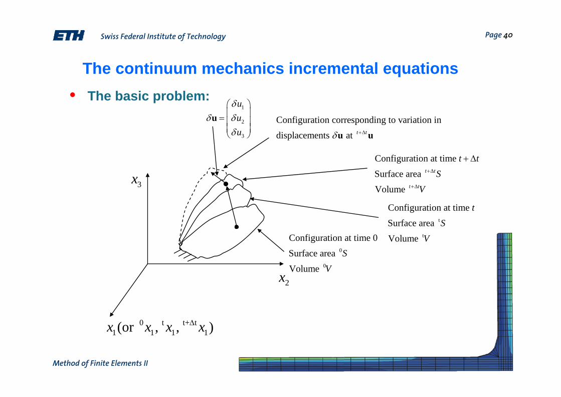
The continuum mechanics incremental equations• The basic problem:

We want to establish the solution using an incremental formulation

The equilibrium must be established for the considered body in its current configuration

In proceeding we adopt a Lagrangian formulation where we track the movement of all particles of the body (located in a Cartesian coordinate system)

Another approach would be an Eulerian formulation where the motion of material through a stationary control volume is considered



The continuum mechanics incremental equations• The basic problem:

0 t t+ t1 1 1 1(or , , )x x x xΔ

2x

3x

0

0

Configuration at time 0Surface area Volume

SV

t

t

Configuration at time Surface area Volume

tS

V


t t

t t

t tS

V

+Δ

+Δ

+ Δ

Configuration corresponding to variation in displacements at t tδ +Δu u

1

2

3

uuu

δδ δ

δ

⎛ ⎞⎜ ⎟= ⎜ ⎟⎜ ⎟⎝ ⎠

u



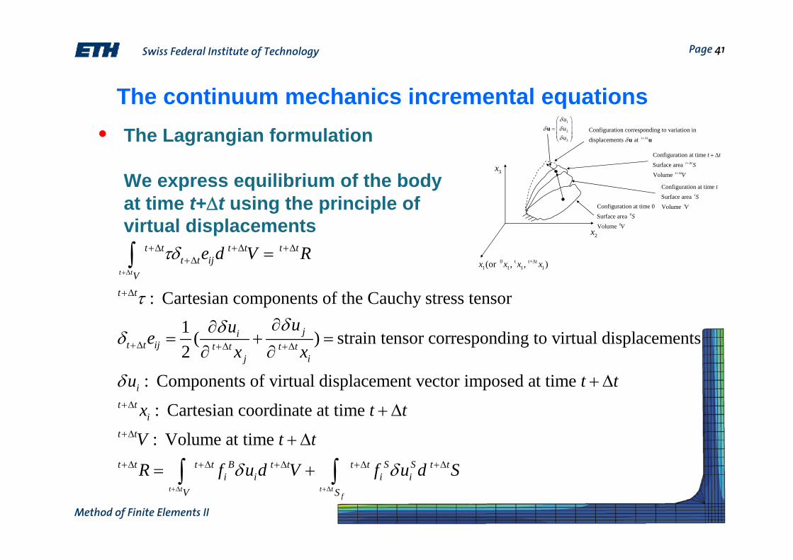
The continuum mechanics incremental equations• The Lagrangian formulation

We express equilibrium of the body at time t+Δt using the principle of virtual displacements

0 t t+ t1 1 1 1(or , , )x x x xΔ

2x

3x

0

0


SV

t

t


tS

V


t t

t t

t tS

V

+Δ

+Δ

+ Δ


1

2

3

uuu

δδ δ

δ

⎛ ⎞⎜ ⎟= ⎜ ⎟⎜ ⎟⎝ ⎠

u

: Cartesian components of the Cauchy stress tensor1 ( ) strain tensor corresponding to virtual displacements2

: Components of virtua

t t

t t t t t tt t ij

V

t t

jit t ij t t t t

j i

i

e d V R

uuex x

u

τδ

τδδδ

δ

+Δ

+Δ +Δ +Δ+Δ

+Δ

+Δ +Δ +Δ

=

∂∂= + =

∂ ∂

∫

l displacement vector imposed at time

: Cartesian coordinate at time

: Volume at time

t t t tf

t ti

t t

t t t t B t t t t S S t ti i i i

V S

t t

x t t

V t t

R f u d V f u d Sδ δ+Δ +Δ

+Δ

+Δ

+Δ +Δ +Δ +Δ +Δ

+ Δ

+ Δ

+ Δ

= +∫ ∫




We express equilibrium of the body at time t+Δt using the principle of virtual displacements

0 t t+ t1 1 1 1(or , , )x x x xΔ

2x

3x

0

0


SV

t

t


tS

V


t t

t t

t tS

V

+Δ

+Δ

+ Δ


1

2

3

uuu

δδ δ

δ

⎛ ⎞⎜ ⎟= ⎜ ⎟⎜ ⎟⎝ ⎠

u

where: externally applied forces per unit volume

: externally applied surface tractions per unit surface

: surface at time

t t t tf

t t t t B t t t t S S t ti i i i

V S

t t Bi

t t Si

t tf

R f u d V f u d S

f

f

S t t

u

δ δ

δ

+Δ +Δ

+Δ +Δ +Δ +Δ +Δ

+Δ

+Δ

+Δ

= +

+ Δ

∫ ∫

: evaluated at the surface S t ti i fu Sδ +Δ




We recognize that our derivations from linear finite element theory are unchanged – but applied to the body in the configuration at time t+Δt



The continuum mechanics incremental equations• In the further we introduce an appropriate notation:

0

0

0

Coordinates and displacements are related as:

Increments in displacements are related as:

Reference configurations are indexed as e.g.: where the lower

t ti i i

t t t ti i i

t t tt i i i

t t Si

x x u

x x u

u u u

f

+Δ +Δ

+Δ

+Δ

= +

= +

= −

00

0 , ,0

left index indicates the reference configuration

=

Differentiation is indexed as:

,

t t t tij t t ij

t tt t i m

i j t t m n t tj n

u xu xx x

τ τ+Δ +Δ+Δ

+Δ+Δ

+Δ +Δ

∂ ∂= =

∂ ∂

Documents

The Finite Element Method for the Analysis of Non …webarchiv.ethz.ch/ibk/emeritus/fa/education/FE_II/Lecture_1.pdf · Swiss Federal Institute of Technology Page 1 Method of Finite