Embed Size (px)
Citation preview
851-0585-04L – Modelling and Simulating851 0585 04L Modelling and Simulating Social Systems with MATLAB
Lesson 3 – Dynamical Systems
Anders Johansson and Wenjian Yu
2010-03-08© ETH Zürich |

ProjectsImplementation of a model from theImplementation of a model from the Social-Science literature in MATLAB.Carried out in pairs.The projects will be assigned next week:The projects will be assigned next week:March 15, 2010
2010-03-08 A. Johansson & W. Yu / [email protected] [email protected] 2
Lesson 3 - ContentsDifferential EquationsDifferential Equations
Dynamical SystemsPendulumLorenz attractorLotka-Volterra equationsEpidemics: Kermack-McKendrick modelEpidemics: Kermack McKendrick model
Exercises
2010-03-08 A. Johansson & W. Yu / [email protected] [email protected] 3
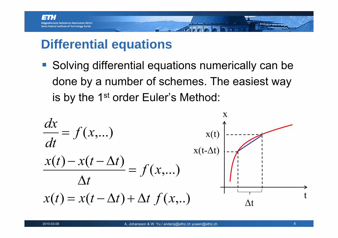
Differential equationsSolving differential equations numerically can beSolving differential equations numerically can be done by a number of schemes. The easiest way is by the 1st order Euler’s Method:
dx
,...)(xfdtdx
= x(t)
,...)()()( xfttxtxdt
=Δ−−
x(t-Δt)
)()()(
,...)(
xftttxtx
xft
Δ+Δ−=Δ
tΔ
2010-03-08 A. Johansson & W. Yu / [email protected] [email protected] 4
,..)()()( xftttxtx Δ+Δ= Δt
Dynamical systemsA dynamical system is a mathematicalA dynamical system is a mathematical description of the time dependence of a point in a space.
A dynamical system is described by a set ofA dynamical system is described by a set of linear/non-linear differential equations.
Even though an analytical treatment of dynamical systems is often complicated, y y p ,obtaining a numerical solution is straight forward
2010-03-08 A. Johansson & W. Yu / [email protected] [email protected] 5
forward.
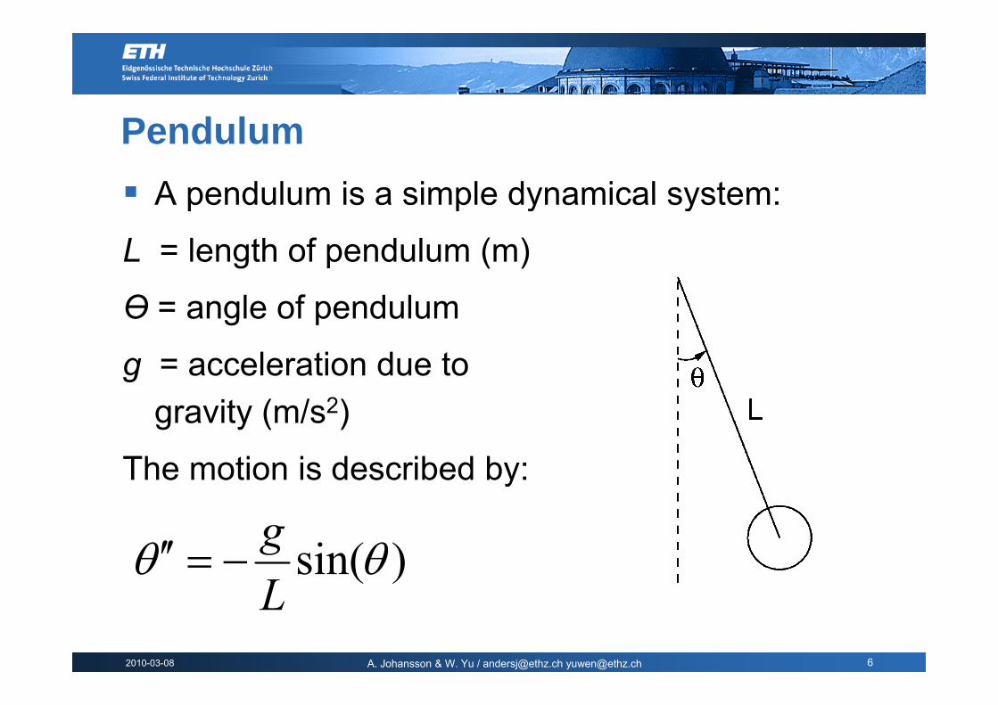
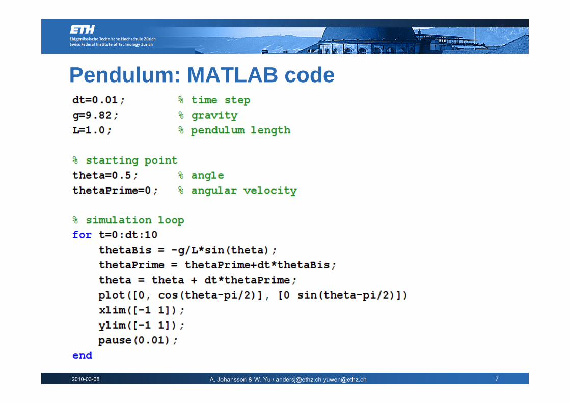
PendulumA pendulum is a simple dynamical system:A pendulum is a simple dynamical system:
L = length of pendulum (m)
ϴ = angle of pendulum
l ti d tg = acceleration due to gravity (m/s2)
The motion is described by:
)sin(θθLg
−=′′
2010-03-08 A. Johansson & W. Yu / [email protected] [email protected] 6
L
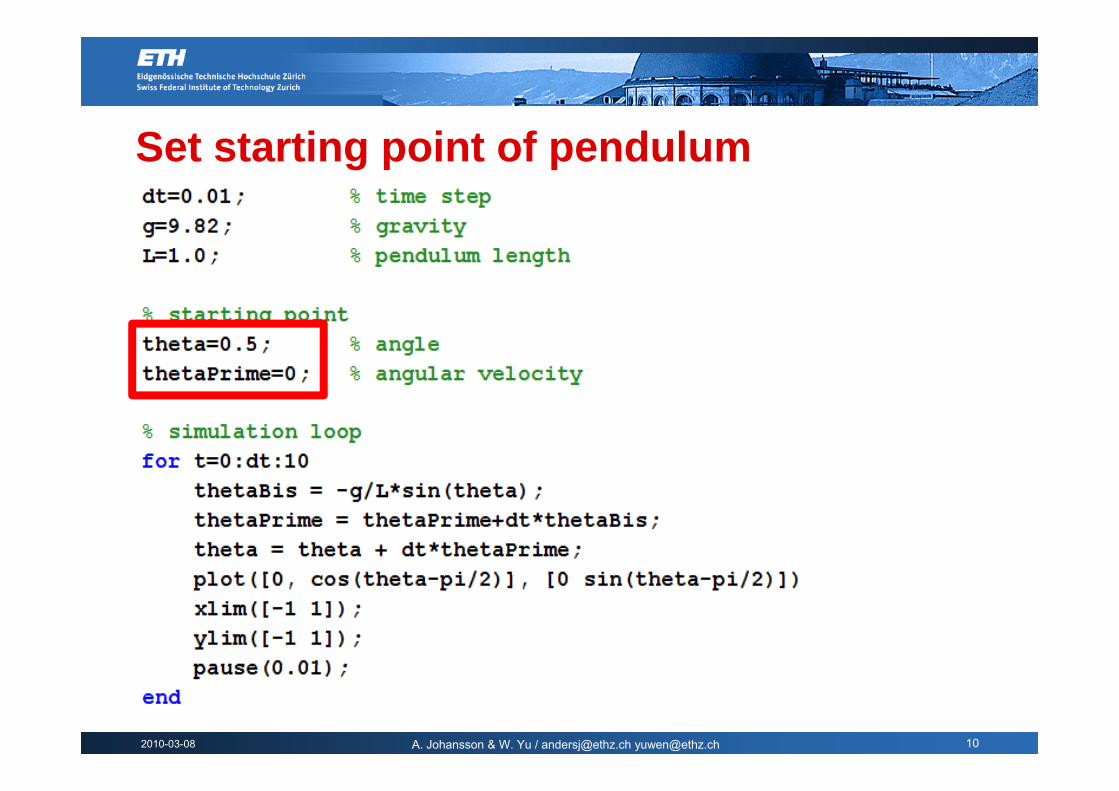
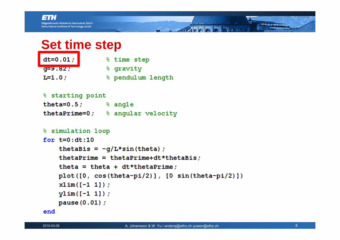
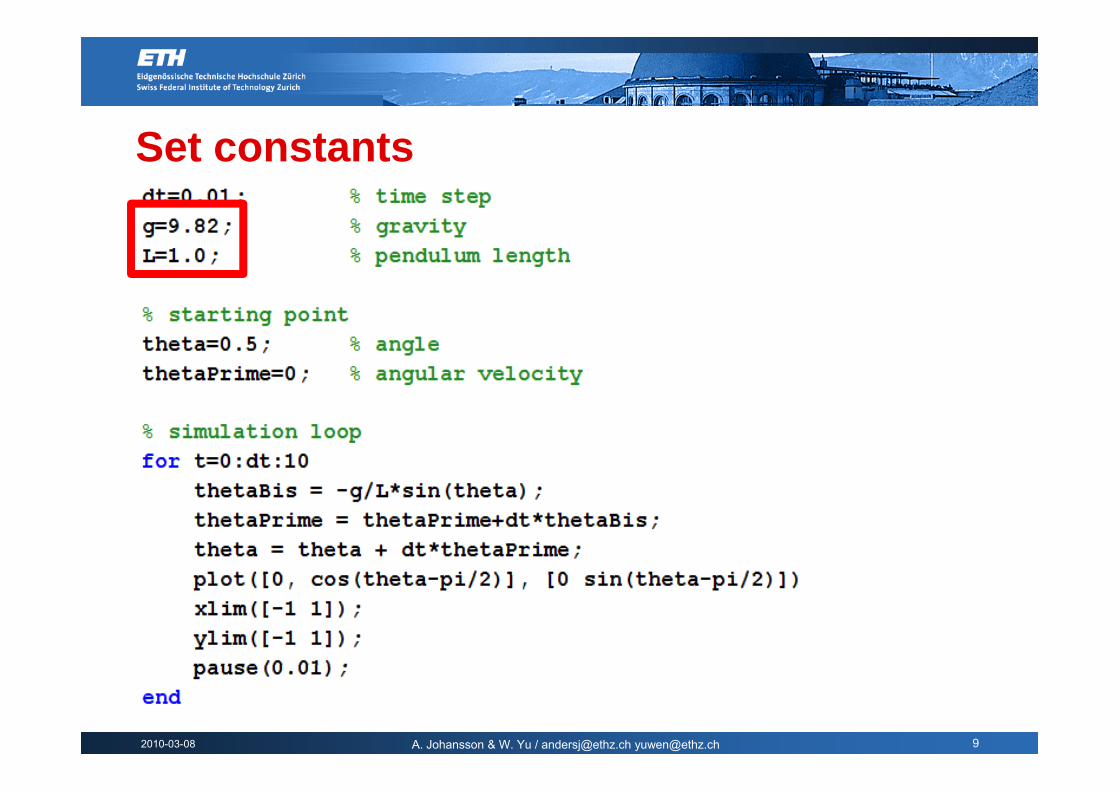
Set starting point of pendulum
2010-03-08 A. Johansson & W. Yu / [email protected] [email protected] 10
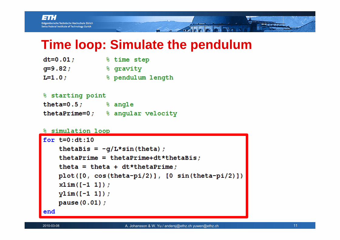
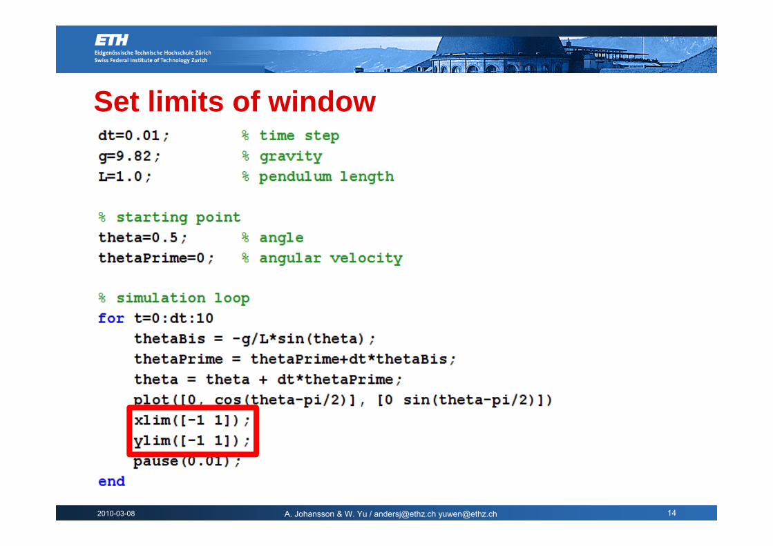
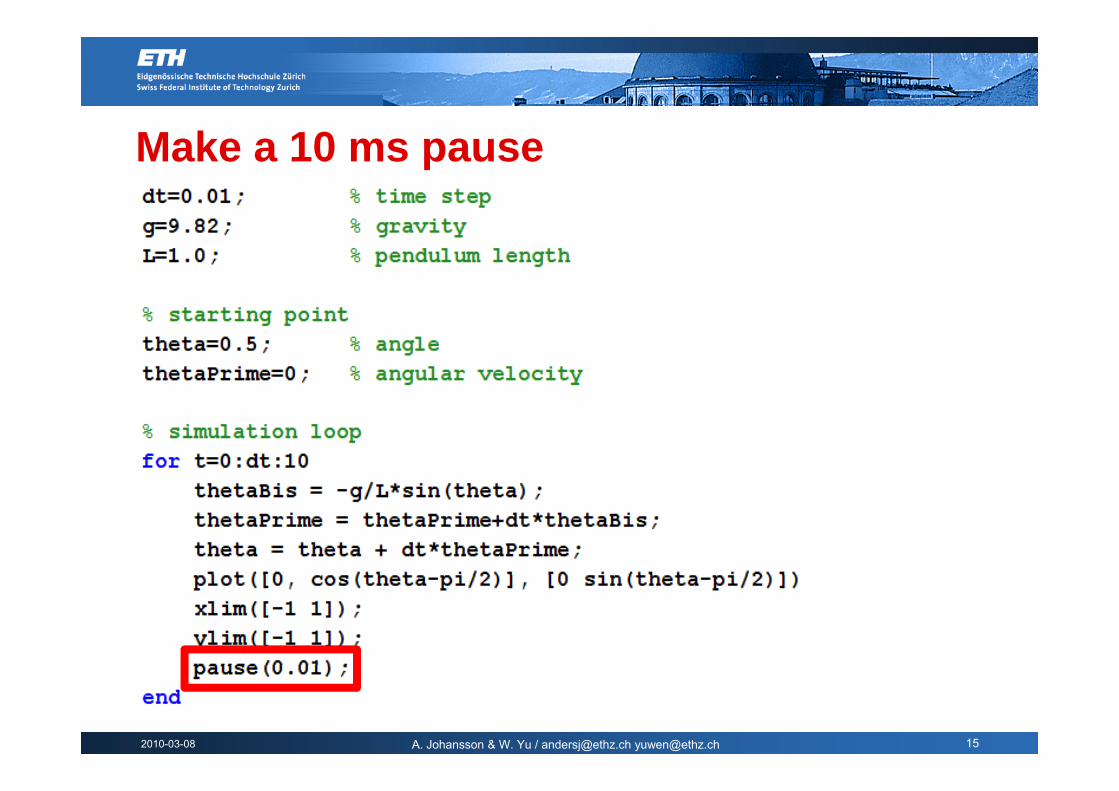
Time loop: Simulate the pendulum
2010-03-08 A. Johansson & W. Yu / [email protected] [email protected] 11
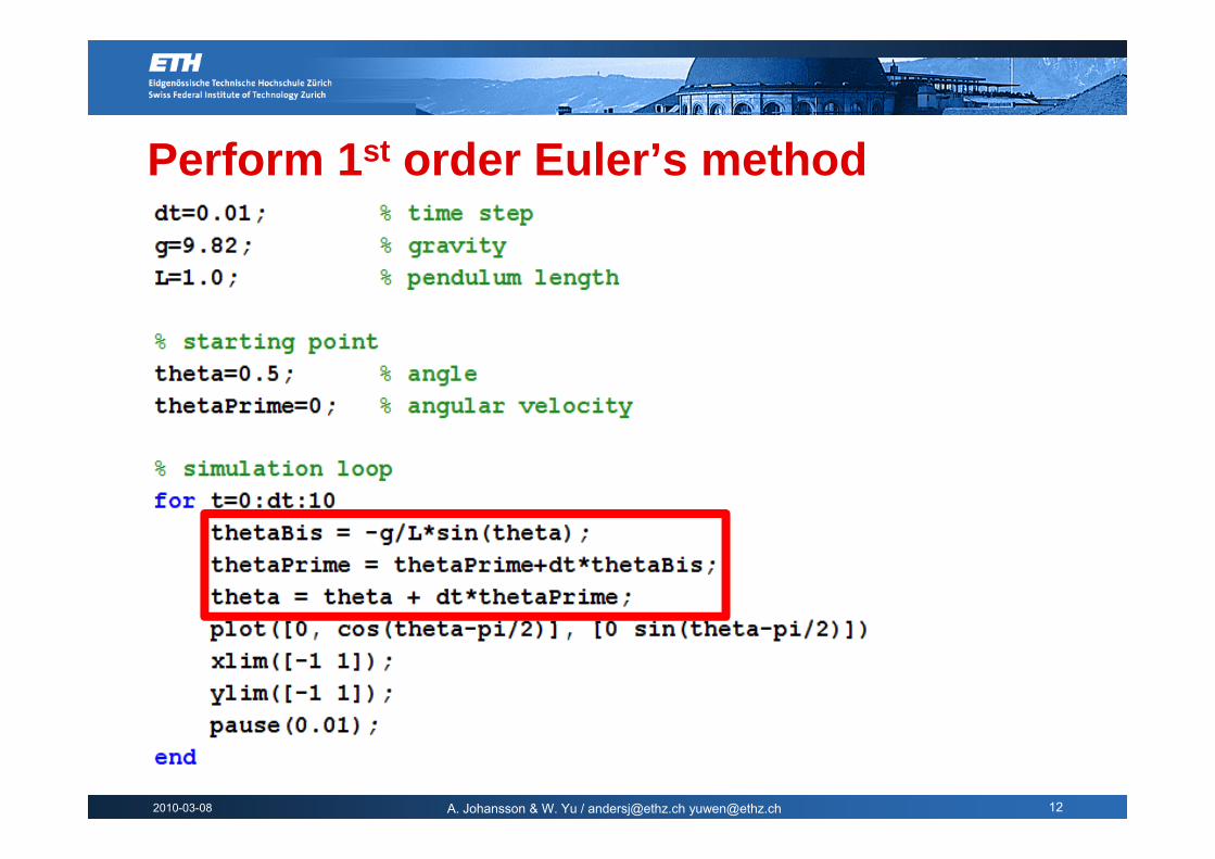
Perform 1st order Euler’s method
2010-03-08 A. Johansson & W. Yu / [email protected] [email protected] 12
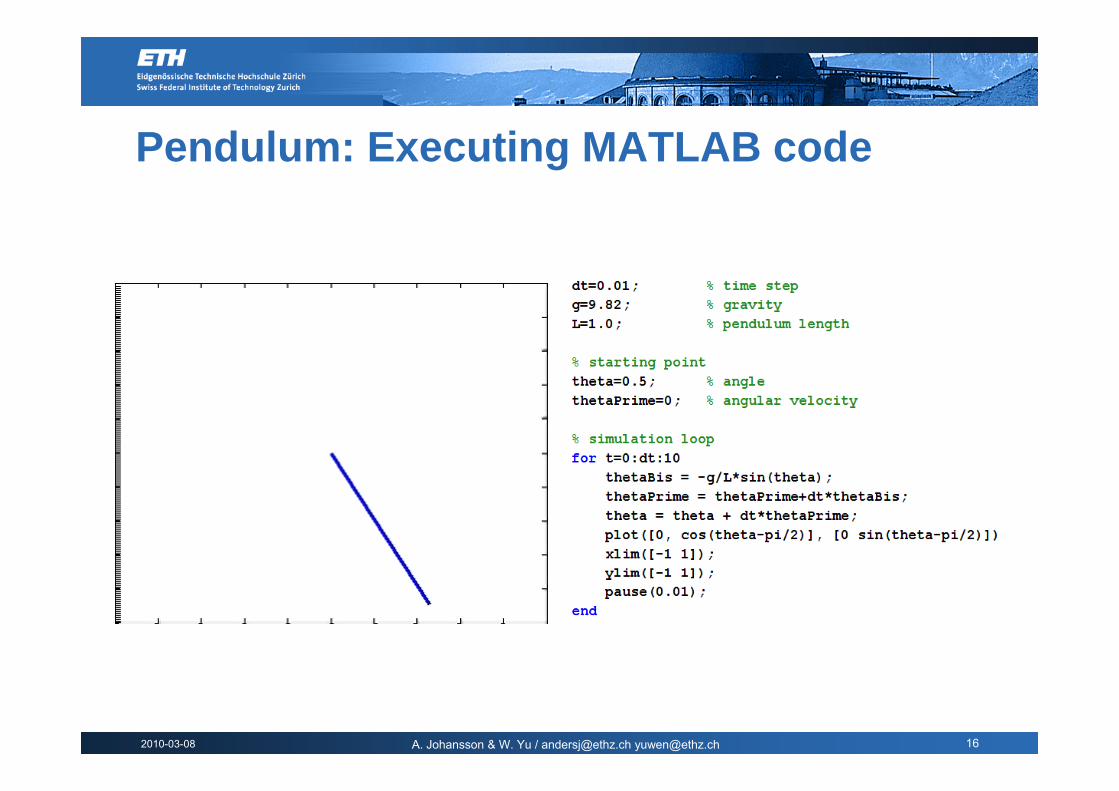
Pendulum: Executing MATLAB code
2010-03-08 A. Johansson & W. Yu / [email protected] [email protected] 16
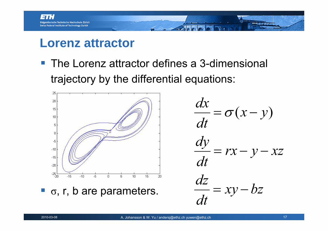
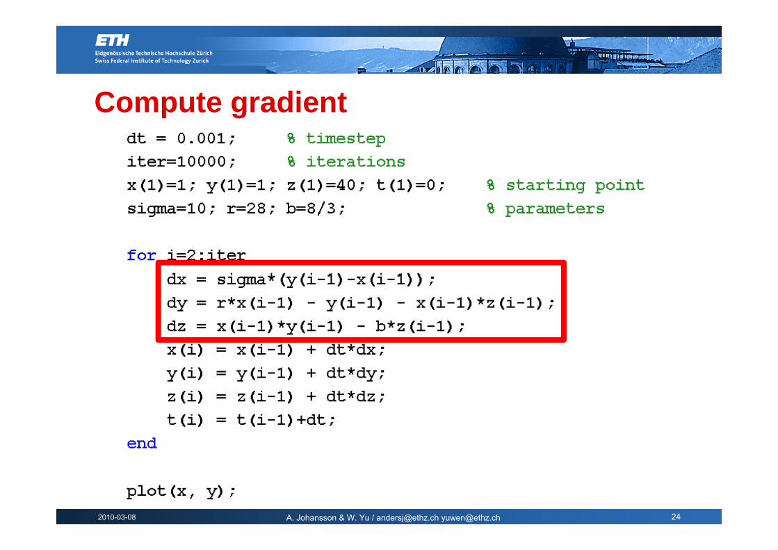
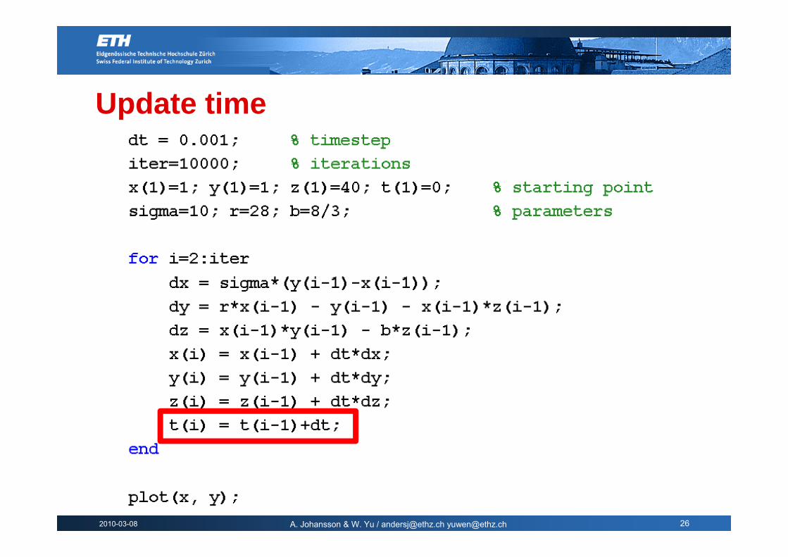
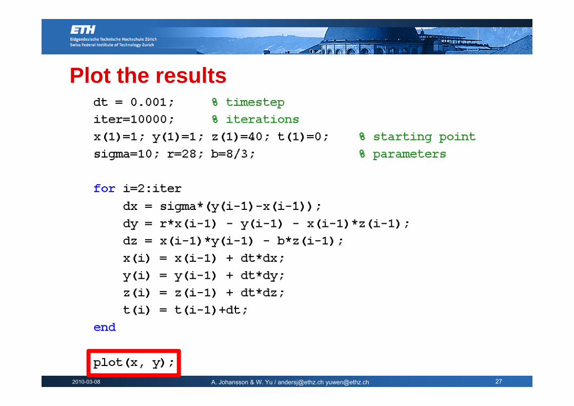
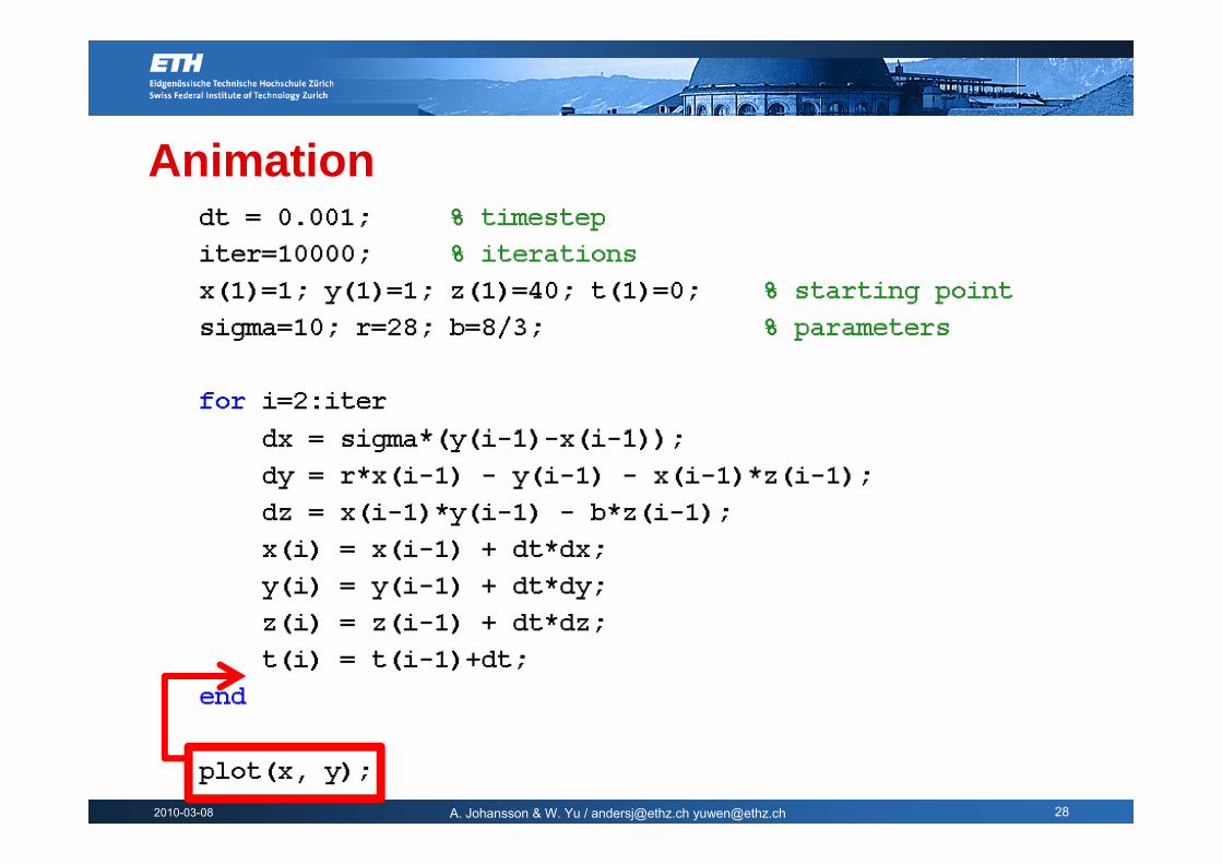
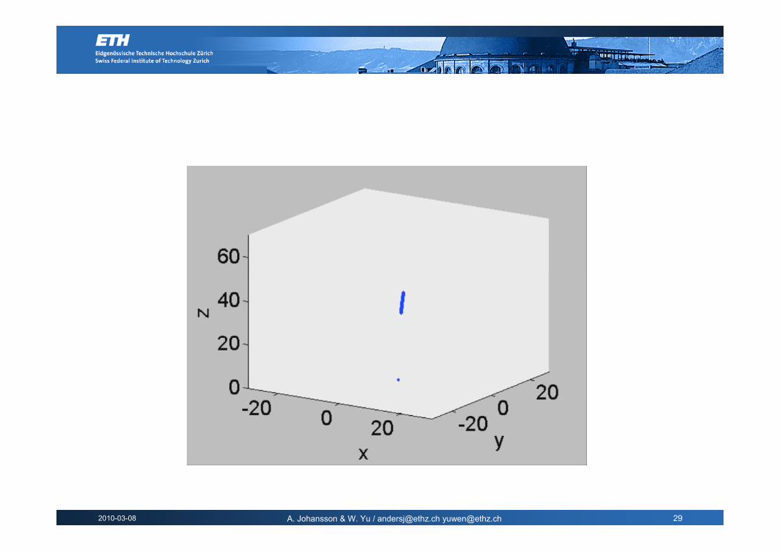
Lorenz attractorThe Lorenz attractor defines a 3 dimensionalThe Lorenz attractor defines a 3-dimensional trajectory by the differential equations:
yxdx−= )(σ
dy
yxdt
)(σ
xzyrxdtdy
−−=
σ, r, b are parameters. bzxydz−=
2010-03-08 A. Johansson & W. Yu / [email protected] [email protected] 17
σ, r, b are parameters. ydt

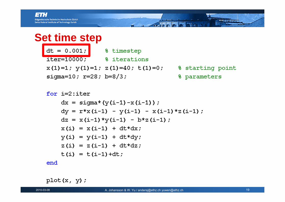
Lorenz attractor: MATLAB code
2010-03-08 A. Johansson & W. Yu / [email protected] [email protected] 18
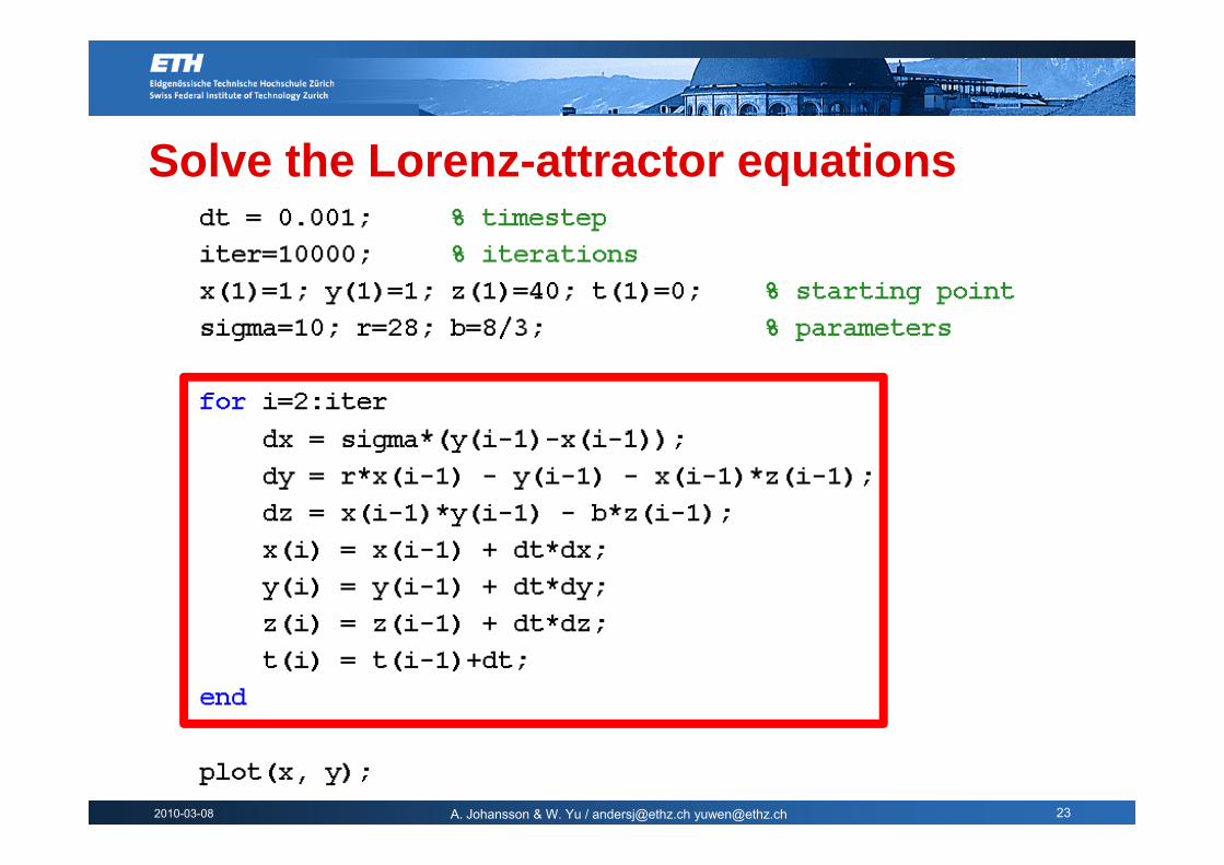
Solve the Lorenz-attractor equations
2010-03-08 A. Johansson & W. Yu / [email protected] [email protected] 23

Perform 1st order Euler’s method
2010-03-08 A. Johansson & W. Yu / [email protected] [email protected] 25
2010-03-08 A. Johansson & W. Yu / [email protected] [email protected] 29

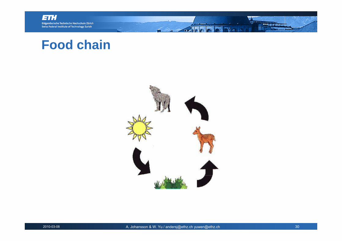
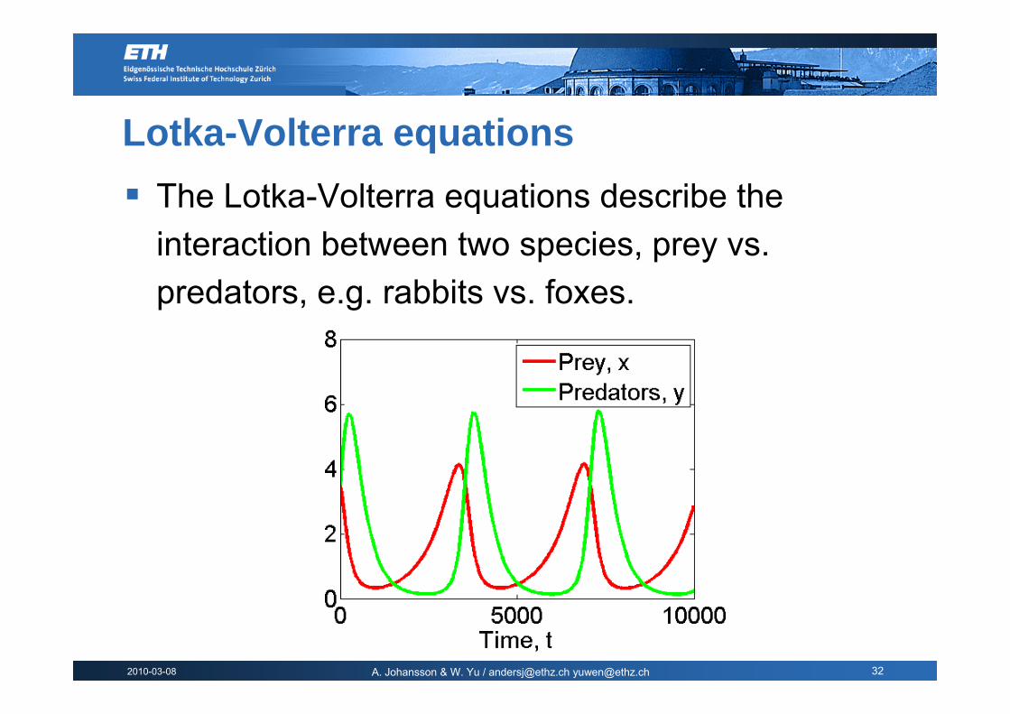
Lotka-Volterra equationsThe Lotka Volterra equations describe theThe Lotka-Volterra equations describe the interaction between two species, prey vs. predators, e.g. rabbits vs. foxes.
x: number of preyy: number of predators
)( yxdtdx βα −=
y: number of predatorsα, β, γ, δ: parameters
)(dydt
δ )( xydty δγ −−=
2010-03-08 A. Johansson & W. Yu / [email protected] [email protected] 31
Lotka-Volterra equationsThe Lotka Volterra equations describe theThe Lotka-Volterra equations describe the interaction between two species, prey vs. predators, e.g. rabbits vs. foxes.
2010-03-08 A. Johansson & W. Yu / [email protected] [email protected] 32
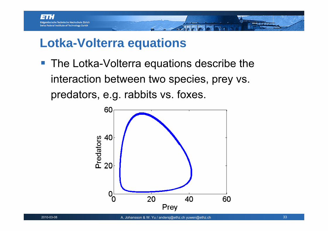
Lotka-Volterra equationsThe Lotka Volterra equations describe theThe Lotka-Volterra equations describe the interaction between two species, prey vs. predators, e.g. rabbits vs. foxes.
2010-03-08 A. Johansson & W. Yu / [email protected] [email protected] 33
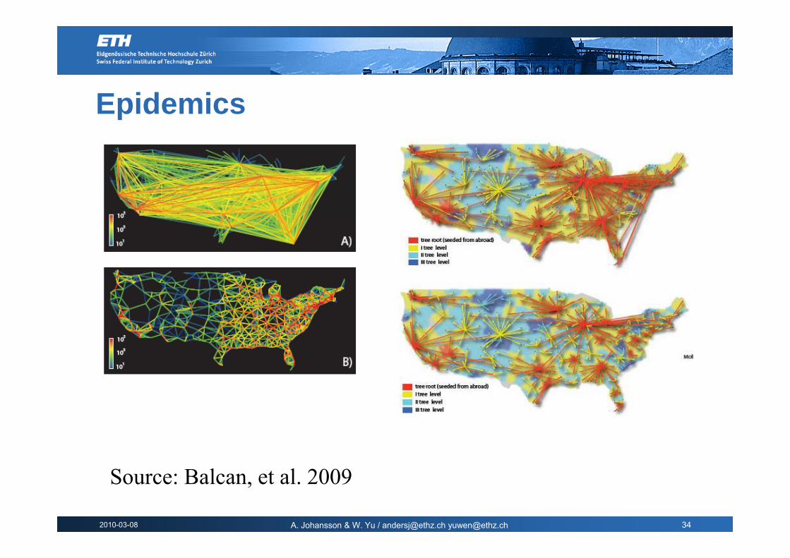
Epidemics
S l l 2009
2010-03-08 A. Johansson & W. Yu / [email protected] [email protected] 34
Source: Balcan, et al. 2009
SIR modelA model for epidemics is the SIR model whichA model for epidemics is the SIR model, which describes the interaction between Susceptible, Infected and Removed (immune) persons, for a given disease. g
2010-03-08 A. Johansson & W. Yu / [email protected] [email protected] 35
Kermack-McKendrick modelof diseases like the plague and cholera Aof diseases like the plague and cholera. A popular SIR model is the Kermack-McKendrick model. The model was proposed for explaining the spreading p g
The model assumes:A t t l ti iA constant population size.A zero incubation period.The duration of infectivity is as long as the duration of the clinical disease.
2010-03-08 A. Johansson & W. Yu / [email protected] [email protected] 36
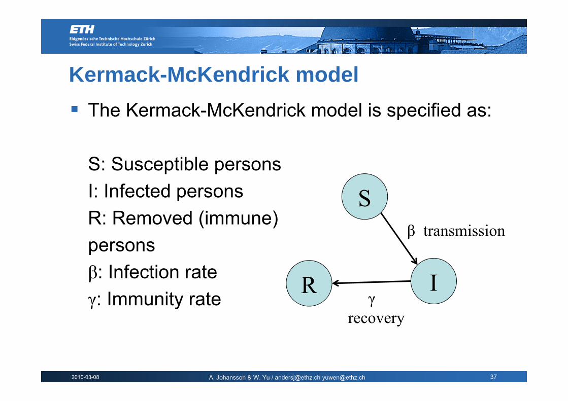
Kermack-McKendrick modelThe Kermack McKendrick model is specified as:The Kermack-McKendrick model is specified as:
S: Susceptible personsI: Infected persons SpR: Removed (immune) persons
Sβ transmission
personsβ: Infection rate IRγ: Immunity rate R γ
recovery
2010-03-08 A. Johansson & W. Yu / [email protected] [email protected] 37

Kermack-McKendrick modelThe Kermack McKendrick model is specified as:The Kermack-McKendrick model is specified as:
S: Susceptible personsI: Infected persons )()( tStI
dtdS β−=p
R: Removed (immune) persons )()()( tItStIdI
dt
γβ=personsβ: Infection rate
)()()(
dR
tItStIdt
γβ −=
γ: Immunity rate )( tIdtdR γ=
2010-03-08 A. Johansson & W. Yu / [email protected] [email protected] 38

Kermack-McKendrick modelThe Kermack McKendrick model is specified as:The Kermack-McKendrick model is specified as:
S: Susceptible personsI: Infected personspR: Removed (immune) personspersonsβ: Infection rateγ: Immunity rate
2010-03-08 A. Johansson & W. Yu / [email protected] [email protected] 39

Exercise 1Implement and simulate the KermackImplement and simulate the Kermack-McKendrick model in MATLAB.
Use the starting values: gS=I=500, R=0, β=0.0001, γ =0.01
Slides/exercises: www.soms.ethz.ch/matlab
2010-03-08 A. Johansson & W. Yu / [email protected] [email protected] 40
(Download only possible with Firefox!)
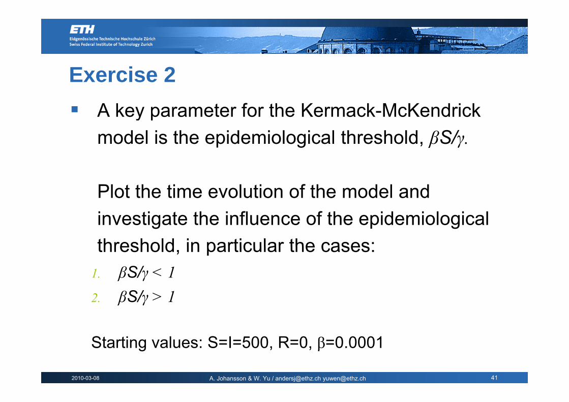
Exercise 2A key parameter for the Kermack McKendrickA key parameter for the Kermack-McKendrick model is the epidemiological threshold, βS/γ.
Plot the time evolution of the model and investigate the influence of the epidemiological threshold in particular the cases:threshold, in particular the cases:
1. βS/γ < 1βS/ 12. βS/γ > 1
St ti l S I 500 R 0 β 0 0001
2010-03-08 A. Johansson & W. Yu / [email protected] [email protected] 41
Starting values: S=I=500, R=0, β=0.0001
Exercise 3 - optionalImplement the Lotka Volterra model andImplement the Lotka-Volterra model and investigate the influence of the timestep, dt.
How small must the timestep be in order for the 1st order Eulter‘s method to give reasonable1 order Eulter s method to give reasonable accuracy?
Check in the MATLAB help how the functions ode23, ode45 etc, can be used for solving , , gdifferential equations.
2010-03-08 A. Johansson & W. Yu / [email protected] [email protected] 42