THE FACTORIZATION MATRICES* - numerical.rl.ac.uk · Therefore, if Gauss-Jordan elimination is performed by applying ... is formed naturally when LUor Gauss-Jordan factorization is

SIAM J. ScI. STAT. COMPUT.Vol. 11, No. 5, pp. 913-927, September 1990 006

USE OF THE p4 AND pS ALGORITHMS FOR IN-COREFACTORIZATION OF SPARSE MATRICES*

M. ARIOLI?, I. S. DUFFS, N. I. M. GOULDt, AND J. K. REID$

Abstract. Variants of the p4 algorithm of Hellerman and Rarick and the p5 algorithm of Erisman,Grimes, Lewis, and Poole, used for generating a bordered block triangular form for the in-core solution ofsparse sets of linear equations, are considered.

A particular concern is with maintaining numerical stability. Methods for ensuring stability and theextra cost that they entail are discussed.

Different factorization schemes are also examined. The uses of matrix modification and iterativerefinement are considered, and the best variant is compared with an established code for the solution ofunsymmetric sparse sets of linear equations. The established code is usually found to be the most effectivemethod.

Key words, sparse matrices, tearing, linear programming, bordered block triangular form, Gaussianelimination, numerical stability

AMS(MOS) subject classifications. 65F50, 65K05, 65F05

1. Introduction. For solving sparse unsymmetric sets of linear equations

(1.1) Ax=b,

Hellerman and Rarick (1971) introduced an algorithm for permuting A to borderedblock triangular form, which they called the preassigned pivot procedure (p3). A littlelater, Hellerman and Rarick (1972) suggested that the matrix should initially bepermuted to block triangular form and that the p3 algorithm should be applied to eachdiagonal block; they called this the partitioned preassigned pivot procedure (p4). Apotential problem with both of these algorithms is that, when Gaussian elimination isapplied to the reordered matrix, some of the pivots may be small or even zero. Thisleads to numerical instability or breakdown of the algorithm. They intended that smallpivots should be avoided, but the published explanation of their algorithm is lackingin detail.

Saunders (1976, p. 222) used column interchanges to avoid this difficulty. Erisman,Grimes, Lewis, and Poole (1985) proposed a cautious variant of p4 that they calledthe precautionary partitioned preassigned pivot procedure (pS). p5 avoids structurallyzero pivots away from the border, but does not address problems associated with smallpivots.

Erisman et al. (1985), (1987) performed some extensive numerical tests using asa benchmark the Harwell code MA28 (Duff (1977), Duff and Reid (1979)), which usesthe pivotal strategy of Markowitz (1957) and a relative pivot test

(k) > (k)(1.2) lakk U max [akjj>k

* Received by the editors December 28, 1987, accepted for publication (in revised form) July 24, 1989.t Centre Europ6en de Recherche et de Formation Avanc6e en Calcul Scientifique, 42 Avenue G. Coriolis,

31057 Toulouse Cedex, France.Computer Science and Systems Division, Harwell Laboratory, Oxfordshire OX11 0RA, United King-

dom. Present address, Central Computing Department, Atlas Centre, Rutherford Appleton Laboratory,Oxfordshire OXll 0QX, United Kingdom.

This research was performed while this author was visiting Harwell Laboratory and was funded bya grant from the Italian National Council of Research (CNR), Istituto di Elaborazione dell’Informazione,CNR, via. S. Maria 46, 56100 Pisa, Italy.

913

914 M. ARIOLI, I. S. DUFF, N. I. M. GOULD, AND J. K. REID

(k) of the kth pivot row. Here u is a preassigned factor, usually seton the elements a kj

to 0.1. The Erisman et al. (1985) tests showed their p4 algorithm encountering zeropivots and therefore failing in more than half the test cases. This illustrates thatprovision for reordering is an essential part of a reliable algorithm. Erisman et al.(1987) found a full 2 x 2 block that was exactly singular, which illustrates that it is notsufficient to ensure that the diagonal entries are structurally nonzero. They concluded(1987) in favour of the standard Markowitz approach, as represented by MA28.

To make this paper self-contained, we summarize the properties of the reductionto block triangular form in 2 and of the p5 and p4 algorithms in 3 and 4. Fordetailed descriptions, we refer the reader to Duff, Erisman, and Reid (1986) or Erismanet al. (1985). Both algorithms permute the matrix to a form that is lower triangularwith a few "spike columns" projecting into the upper-triangular part. A practicalimplementation of p4 or p5 needs some provision for, reordering to avoid small pivots.We consider this in 5. We have constructed an experimental code to explore theseideas, and the results are presented in 6. Finally, we present conclusions in 7.

We assume throughout the paper that there is enough main storage for thecomputation to be performed without the use of any form of auxiliary storage.

2. Block triangular matrices. Both the p4 and the P5 algorithms start by permutingthe matrix to block triangular form

AllA21 A22

(2.1) A31 A32 A33

AN! AN2 AN3which allows the system of linear equations

ANN

(2.2) Ax=b

to be solved by block forward substitution

i-1

(2.3) Aiix, b,- Ajxj, i= 1, 2,..., N.j=l

We assume that each block A, is irreducible, that is it cannot itself be permuted toblock triangular form. There are well-established and successful algorithms for reducinga matrix to this form (see Duff et al. (1986), Chap. 6, for example), and good softwareis available. It is the treatment of the blocks A, that is our concern here.

Because we will subsequently perform a block decomposition of the A, blocks,we will use the graph theoretic equivalent term "strong component" to identify a blockA, in the following text.

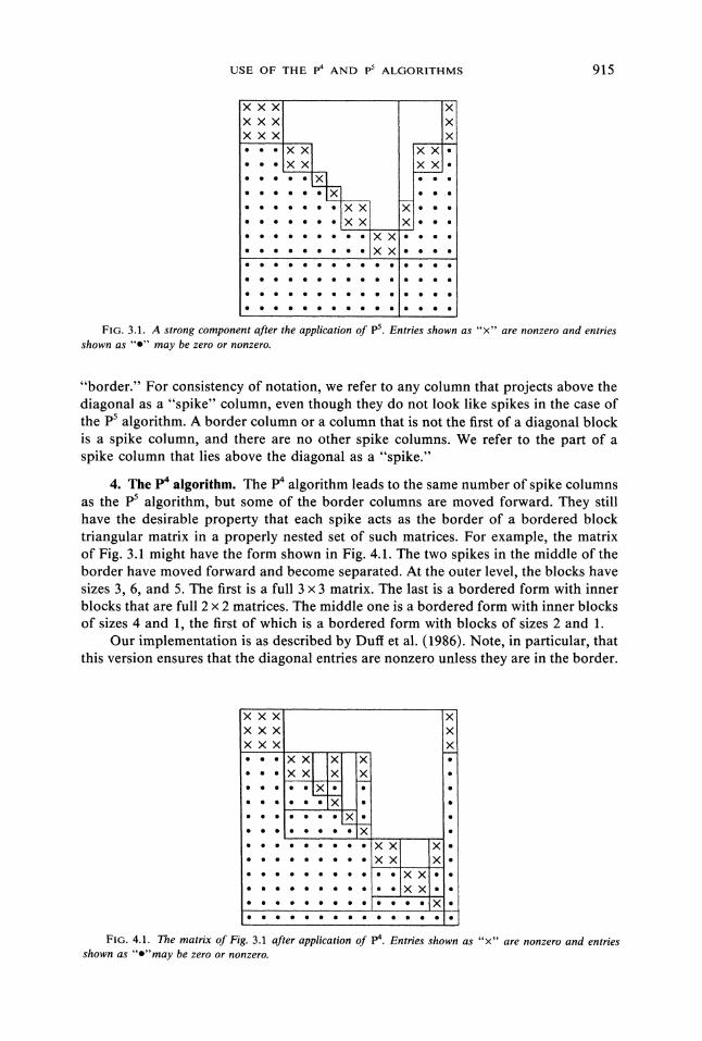
3. The pS algorithm. The P5 algorithm (Erisman et al. (1985)) first permutes thematrix to block triangular form and then further permutes each strong component tothe form illustrated in Fig. 3.1. The general form is of a matrix

where B is block lower triangular with full diagonal blocks and each column of C hasa leading block of nonzero entries in the rows of a diagonal block of B and extendsupwards at least as far as the preceding column. We refer to the columns of (c) as the

USE OF THE p4 AND p5 ALGORITHMS 915

xxxXXXXXXooo,-,XX

X,,,,oooXX,,,,,,,XX

XXX

XX,xx,

XX

FIG. 3.1. A strong component @er the application pS. Entries shown as "x" are nonzero and entriesshown as "o" may be zero or nonzero.

"border." For consistency of notation, we refer to any column that projects above thediagonal as a "spike" column, even though they do not look like spikes in the case ofthe p5 algorithm. A border column or a column that is not the first of a diagonal blockis a spike column, and there are no other spike columns. We refer to the part of aspike column that lies above the diagonal as a "spike."

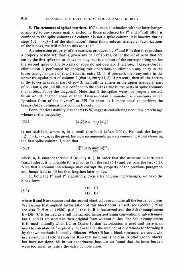
4. The p4 algorithm. The p4 algorithm leads to the same number of spike columnsas the P5 algorithm, but some of the border columns are moved forward. They stillhave the desirable property that each spike acts as the border of a bordered blocktriangular matrix in a properly nested set of such matrices. For example, the matrixof Fig. 3.1 might have the form shown in Fig. 4.1. The two spikes in the middle of theborder have moved forward and become separated. At the outer level, the blocks havesizes 3, 6, and 5. The first is a full 3 x 3 matrix. The last is a bordered form with innerblocks that are full 2 x 2 matrices. The middle one is a bordered form with inner blocksof sizes 4 and 1, the first of which is a bordered form with blocks of sizes 2 and 1.

Our implementation is as described by Duff et al. (1986). Note, in particular, thatthis version ensures that the diagonal entries are nonzero unless they are in the border.

XxxXXXXXX

FIG. 4.1. The matrix of Fig. 3.1 after application of p4. Entries shown as "x" are nonzero and entriesshown as "o"may be zero or nonzero.


5. The treatment of spiked matrices. If Gaussian elimination without interchangesis applied to any sparse matrix, including those produced by p4 and pS, all fill-in isconfined to the spike columns (if column j is not a spike column, it is inactive duringsteps 1, 2,...,j-1 of the elimination). Since this produces triangular factorizationsof the blocks, we will refer to this as "LU."

An interesting property of the matrices produced by p4 and P5 is that they producea properly nested set; that is, given any pair of spikes, either the set of rows that arecut by the first spike on or above its diagonal is a subset of the corresponding set forthe second spike or the two sets of rows do not overlap. Therefore, if Gauss-Jordanelimination is performed by applying row operations to eliminate any entry in thelower triangular part of row 2 (that is, entry (2, 1), if present), then any entry in theupper triangular part of column 2 (that is, entry (1, 2), if present), then all the entriesin the lower triangular part of row 3, then all the entries in the upper triangular partof column 3, etc., all fill-in is confined to the spikes (that is, the parts of spike columnsthat project above the diagonal). Note that if the spikes were not properly nested,fill-in would lengthen some of them. Gauss-Jordan elimination is sometimes called"product form of the inverse" or PFI for short. It is more usual to perform theGauss-Jordan eliminations column by column.

For numerical stability, Saunders (1976) suggests considering a column interchangewhenever the inequality

is not satisfied, where ul is a small threshold (often 0.001). He took the largest(k)a kj j k, ", n, as the pivot, but now recommends (private communication) choosing

the first spike column, l, such that

(k)[ > U2 max [a (k)l(5.2) lakl ’= j>-_kkj I,

where uz is another threshold (usually 0.1), in order that the structure is corruptedleast. Indeed, it is possible for a pivot to fail the test (5.1) and yet pass the test (5.2).Note that a column interchange may corrupt the property of the previous paragraphand hence lead to fill-ins that lengthen later spikes.

In both the p4 and PS algorithms, even after column interchanges, we have theblock form

where B and E are square and the second block column contains all the border columns.We assume that implicit factorization of this block form is used (see George (1974);see also Duff et al. (1986), p. 61); that is, B is factorized and the Schur complementE-DB-1C is formed as a full matrix and factorized using conventional interchanges,but C and D are stored in their original form without fill-ins. The Schur complementis formed naturally when LU or Gauss-Jordan factorization is used and there is noneed to calculate B- explicitly, but note that the number of operations for forming itby the two methods is usually different. Where B has a block structure, we could alsouse an implicit factorization for B so that no fill-in is held in its off-diagonal blocks,but have not done this in our experiments because we found that the inner borderswere too small to justify the extra complication.


6. Numerical experiments. For our numerical experiments, we have taken thematrices studied by Erisman et al. (1985) and included a few more. We have appliedthe Harwell code MA28, which performs Gaussian elimination with the ordering ofMarkowitz (1957) and threshold pivoting. We have used the usual value, u 0.1, forthe threshol.d. MA28 transforms the matrices to block triangular form so that fill-in isconfined to the strong components, but implicit factorization of the strong components(see end of 5) is not available for MA28. We passed the strong components to theHarwell code MC33 that has options for p4 and p5 ordering. We then applied thealgorithms of 5 with (ul, u2) values of (0.1, 0.1), (0.001, 0.1), and (0.0, 0.0).

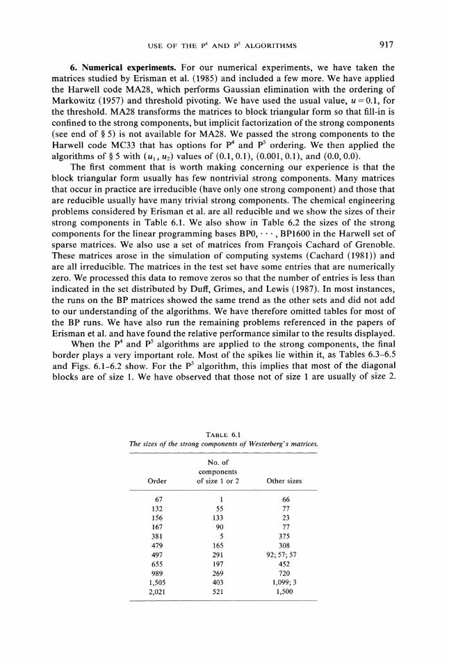
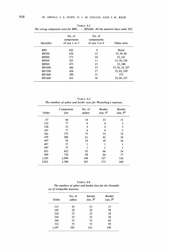
The first comment that is worth making concerning our experience is that theblock triangular form usually has few nontrivial strong components. Many matricesthat occur in practice are irreducible (have only one strong component) and those thatare reducible usually have many trivial strong components. The chemical engineeringproblems considered by Erisman et al. are all reducible and we show the sizes of theirstrong components in Table 6.1. We also show in Table 6.2 the sizes of the strongcomponents for the linear programming bases BP0, , BP1600 in the Harwell set ofsparse matrices. We also use a set of matrices from Francois Cachard of Grenoble.These matrices arose in the simulation of computing systems (Cachard (1981)) andare all irreducible. The matrices in the test set have some entries that are numericallyzero. We processed this data to remove zeros so that the number of entries is less thanindicated in the set distributed by Duff, Grimes, and Lewis (1987). In most instances,the runs on the BP matrices showed the same trend as the other sets and did not addto our understanding of the algorithms. We have therefore omitted tables for most ofthe BP runs. We have also run the remaining problems referenced in the papers ofErisman et al. and have found the relative performance similar to the results displayed.

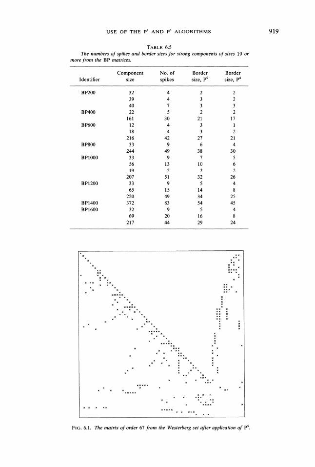
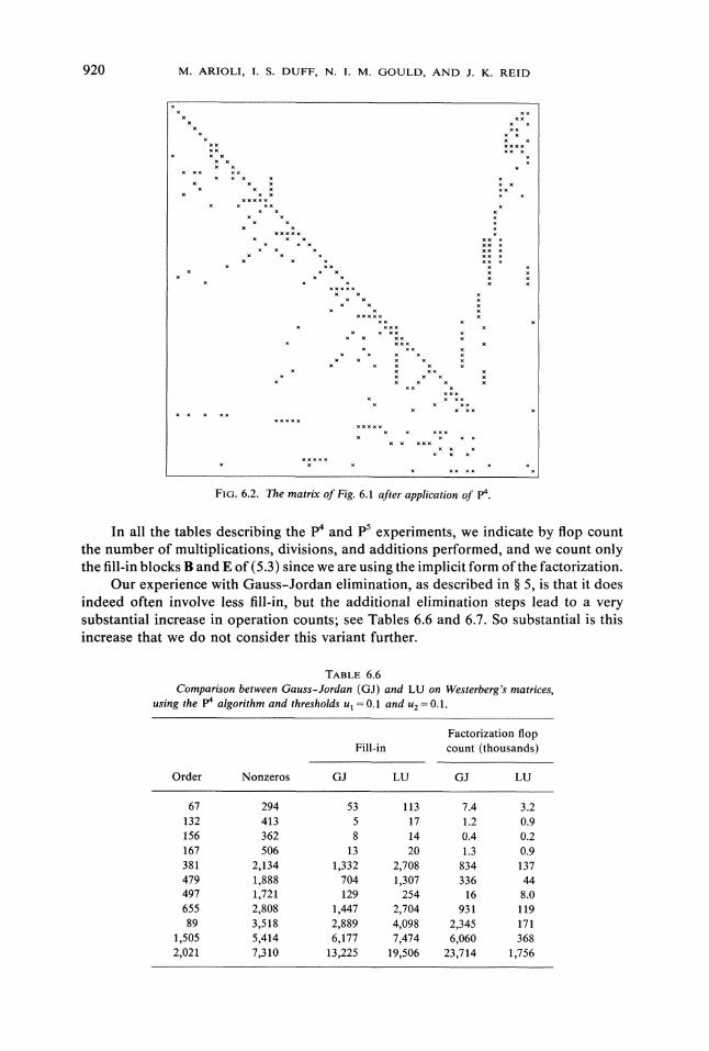
When the p4 and p5 algorithms are applied to the strong components, the finalborder plays a very important role. Most of the spikes lie within it, as Tables 6.3-6.5and Figs. 6.1-6.2 show. For the P5 algorithm, this implies that most of the diagonalblocks are of size 1. We have observed that those not of size 1 are usually of size 2.

TABLE 6.1The sizes of the strong components of Westerberg’s matrices.

No. ofcomponents

Order of size or 2 Other sizes

67 66132 55 77156 133 23167 90 77381 5 375479 165 308497 291 92;57;57655 197 452989 269 7201,505 403 1,099;32,021 521 1,500


TABLE 6.2The strong component sizes for BP0, , BP1600. All the matrices have order 822.

No. of No. ofcomponents components

Identifier of size or 2 of size 3 to 9 Other sizes

BP0 822 0 NoneBP200 658 12 32, 39, 40BP400 575 14 22, 161BP600 523 11 12, 18,216BP800 475 15 33,244BP1000 446 13 33, 56, 19, 207BP1200 426 17 33, 65,220BP1400 390 12 372BP1600 431 16 32, 69,217

TABLE 6.3The numbers of spikes and border sizes for Westerberg’s matrices.

Component No. of Border BorderOrder size spikes size, p5 size, p4

67 66 14 13 11132 77 6 4 3156 23 4 4 3167 77 6 4 3381 375 75 53 52479 308 61 42 38497 92 19 18 16497 57497 57655 452 93 66 54989 720 98 84 77

1,505 1,099 148 127 1162,021 1,500 205 175 160

TABLE 6.4The numbers ofspikes and border sizes for the Grenoble

set of irreducible matrices.

No. of Border BorderOrder spikes size, p5 size, p4

115 19 15 15185 28 28 28216 25 25 24216 25 25 24343 52 52 42512 55 55 50

1,107 283 113 100


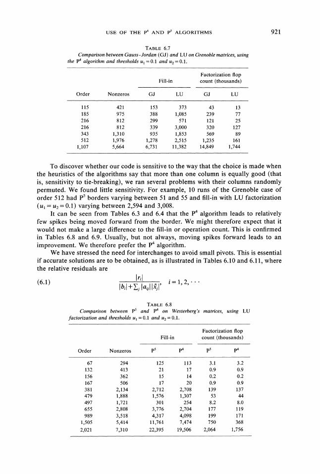
TABLE 6.5The numbers of spikes and border sizes for strong components of sizes 10 or

more from the BP matrices.

Component No. of Border BorderIdentifier size spikes size, p5 size, p4

BP200 32 4 2 239 4 3 240 7 3 3

BP400 22 5 2 2161 30 21 17

BP600 12 4 318 4 3 2

216 42 27 21BP800 33 9 6 4

244 49 38 30BP1000 33 9 7 5

56 13 10 619 2 2 2

207 51 32 26BP1200 33 9 5 4

65 15 14 8220 49 34 25

BP1400 372 83 54 45BP1600 32 9 5 4

69 20 16 8217 44 29 24

FIG. 6.1. The matrix of order 67 from the Westerberg set after application of pS.


FIG. 6.2. The matrix of Fig. 6.1 after application of p4.

In all the tables describing the p4 and p5 experiments, we indicate by flop countthe number of multiplications, divisions, and additions performed, and we count onlythe fill-in blocks B and E of (5.3) since we are using the implicit form ofthe factorization.

Our experience with Gauss-Jordan elimination, as described in 5, is that it doesindeed often involve less fill-in, but the additional elimination steps lead to a verysubstantial increase in operation counts; see Tables 6.6 and 6.7. So substantial is thisincrease that we do not consider this variant further.

TABLE 6.6Comparison between Gauss-Jordan (GJ) and LU on Westerberg’s matrices,

using the p4 algorithm and thresholds u =0.1 and u2 =0.1.

Factorization flopFill-in count (thousands)

Order Nonzeros GJ LU GJ LU

67 294 53 113 7.4 3.2132 413 5 17 1.2 0.9156 362 8 14 0.4 0.2167 506 13 20 1.3 0.9381 2,134 1,332 2,708 834 137479 1,888 704 1,307 336 44497 1,721 129 254 16 8.0655 2,808 1,447 2,704 931 11989 3,518 2,889 4,098 2,345 171

1,505 5,414 6,177 7,474 6,060 3682,021 7,310 13,225 19,506 23,714 1,756


TABLE 6.7Comparison between Gauss-Jordan (GJ) and LU on Grenoble matrices, using

the p4 algorithm and thresholds u 0.1 and u 0.1.


Order Nonzeros GJ LU GJ LU

115 421 153 373 43 13185 975 388 1,085 239 77216 812 299 571 121 25216 812 339 3,000 320 127343 1,310 935 1,853 569 89512 1,976 1,278 2,515 1,235 161

1,107 5,664 6,731 11,382 14,849 1,744

To discover whether our code is sensitive to the way that the choice is made whenthe heuristics of the algorithms say that more than one column is equally good (thatis, sensitivity to tie-breaking), we ran several problems with their columns randomlypermuted. We found little sensitivity. For example, 10 runs of the Grenoble case oforder 512 had p5 borders varying between 51 and 55 and fill-in with LU factorization(ul u2= 0.1) varying between 2,594 and 3,008.

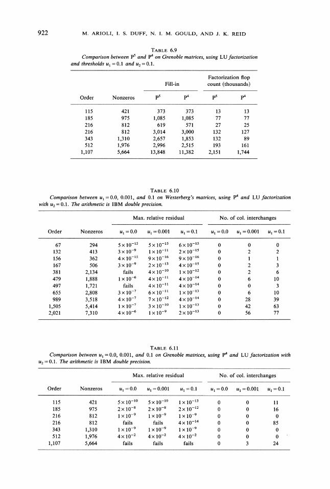
It can be seen from Tables 6.3 and 6.4 that the p4 algorithm leads to relativelyfew spikes being moved forward from the border. We might therefore expect that itwould not make a large difference to the fill-in or operation count. This is confirmedin Tables 6.8 and 6.9. Usually, but not always, moving spikes forward leads to animprovement. We therefore prefer the p4 algorithm.

We have stressed the need for interchanges to avoid small pivots. This is essentialif accurate solutions are to be obtained, as is illustrated in Tables 6.10 and 6.11, wherethe relative residuals are

(6.1)Ib, l+Zlalll’

i--1,2,...

TABLE 6.8Comparison between p5 and p4 on Westerberg’s matrices, using LU

factorization and thresholds u =0.1 and u =0.1.


Order Nonzeros p5 p4 p5 p4

67 294 125 113 3.1 3.2132 413 21 17 0.9 0.9156 362 15 14 0.2 0.2167 506 17 20 0.9 0.9381 2,134 2,712 2,708 139 137479 1,888 1,576 1,307 53 44497 1,721 301 254 8.2 8.0655 2,808 3,776 2,704 177 119989 3,518 4,317 4,098 199 171

1,505 5,414 11,761 7,474 750 368

2,021 7,310 22,395 19,506 2,064 1,756


TABLE 6.9Comparison between p5 and p4 on Grenoble matrices, using LU factorization

and thresholds Ul O. and u O. 1.


Order Nonzeros p5 p4 p5 p4

115 421 373 373 13 13185 975 1,085 1,085 77 77216 812 619 571 27 25216 812 3,014 3,000 132 127343 1,310 2,657 1,853 132 89512 1,976 2,996 2,515 193 161

1,107 5,664 13,848 11,382 2,151 1,744

TABLE 6.10Comparison between u =0.0, 0.001, and 0.1 on Westerberg’s matrices, using p4 and LU factorization

with u2 0.1. The arithmetic is IBM double precision.

Max. relative residual No. of col. interchanges

Order Nonzeros u 0.0 u 0.001 u 0.1 Ul 0.0 ul 0.001 ul 0.1

67 294 5 x 10-15 5 x 10-15 6 x 10-15 0 0 0132 413 3 10-9 10-11 2 10-15 0 2 2156 362 4 x 10-15 9 10-16 9 10-16 0167 506 3 10-9 2 10-13 4 10-15 0 2 3381 2,134 fails 4 10-1 10-12 0 2 6479 1,888 10-6 4 x 10-11 4 x 10-14 0 6 10497 1,721 fails 4 10-11 4 10-14 0 0 3655 2,808 3 10.-7 6 x 10-11 10-13 0 6 10989 3,518 4 10-7 7 10-12 4 x 10-14 0 28 39

1,505 5,414 10-7 3 10-1 10-13 0 42 632,021 7,310 4 10-6 10-9 2X 10-13 0 56 77

TABLE 6.11Comparison between u 0.0, 0.001, and 0.1 on Grenoble matrices, using p4 and LU factorization with

u 0.1. The arithmetic is IBM double precision.

Max. relative residual No. of col. interchanges

Order Nonzeros Ul 0.0 u 0.001 ul 0.1 Ul 0.0 Ul 0.001 ul 0.1

115 421 5 10-l 5 x 10-l 10-13 0 0 11185 975 2x 10-8 2x 10-8 2 10-12 0 0 16216 812 10-9 10-9 10-9 0 0 0216 812 fails fails 4 10-14 0 0 85343 1,310 10-9 10-9 10-9 0 0 0512 1,976 4 10-2 4 10-2 4 10-2 0 0 0

1,107 5,664 fails fails faiIs 0 3 24


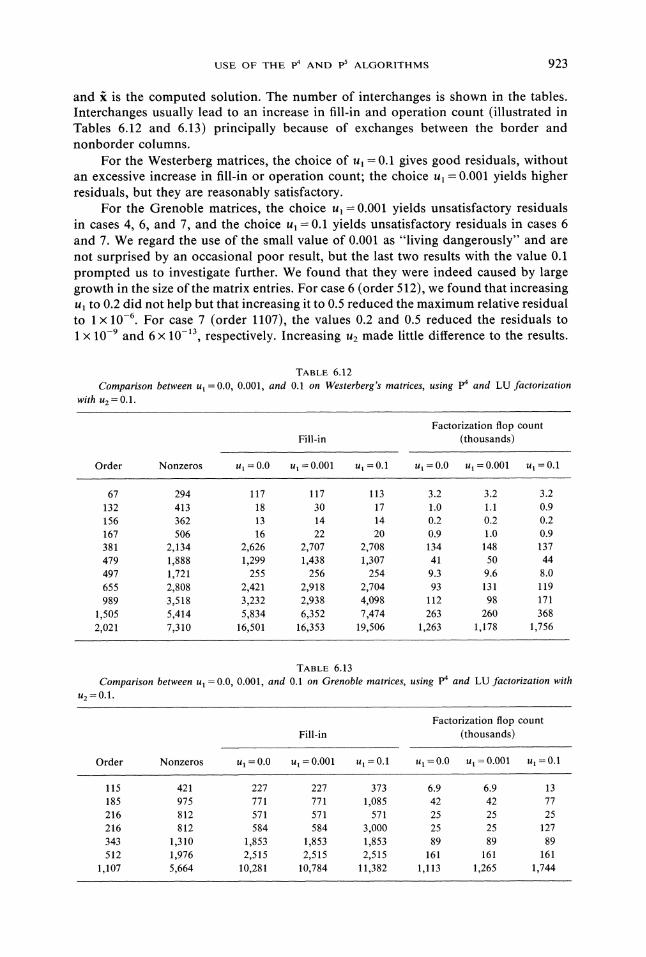
and R is the computed solution. The number of interchanges is shown in the tables.Interchanges usually lead to an increase in fill-in and operation count (illustrated inTables 6.12 and 6.13) principally because of exchanges between the border andnonborder columns.

For the Westerberg matrices, the choice of Ul 0.1 gives good residuals, withoutan excessive increase in fill-in or operation count; the choice Ul 0.001 yields higherresiduals, but they are reasonably satisfactory.

For the Grenoble matrices, the choice Ul=0.001 yields unsatisfactory residualsin cases 4, 6, and 7, and the choice U1-0.1 yields unsatisfactory residuals in cases 6and 7. We regard the use of the small value of 0.001 as "living dangerously" and arenot surprised by an occasional poor result, but the last two results with the value 0.1prompted us to investigate further. We found that they were indeed caused by largegrowth in the size of the matrix entries. For case 6 (order 512), we found that increasingUl to 0.2 did not help but that increasing it to 0.5 reduced the maximum relative residualto 1 x 10-6. For case 7 (order 1107), the values 0.2 and 0.5 reduced the residuals to1 x 10-9 and 6 10-13, respectively. Increasing u2 made little difference to the results.

Comparison between utwith u. O. 1.

TABLE 6.12=0.0, 0.001, and 0.1 on Westerberg’s matrices, using p4 and LU factorization

Factorization flop count

Fill-in (thousands)

Order Nonzeros u 0.0 u 0.001 u 0.1 u 0.0 u 0.001 u 0.1

67 294 117 117 113 3.2 3.2 3.2132 413 18 30 17 1.0 1.1 0.9156 362 13 14 14 0.2 0.2 0.2167 506 16 22 20 0.9 1.0 0.9381 2,134 2,626 2,707 2,708 134 148 137479 1,888 1,299 1,438 1,307 41 50 44497 1,721 255 256 254 9.3 9.6 8.0655 2,808 2,421 2,918 2,704 93 131 119989 3,518 3,232 2,938 4,098 112 98 171

1,505 5,414 5,834 6,352 7,474 263 260 368

2,021 7,310 16,501 16,353 19,506 1,263 1,178 1,756

U2

Comparison between u=0.1.

TABLE 6.130.0, 0.001, and 0.1 on Grenoble matrices, using p4 and LU factorization with

Factorization flop count

Fill-in (thousands)

Order Nonzeros u 0.0 ua 0.001 U 0.1 ut 0.0 u 0.001 u 0.1

115 421 227 227 373 6.9 6.9 13185 975 771 771 1,085 42 42 77216 812 571 571 571 25 25 25216 812 584 584 3,000 25 25 127343 1,310 1,853 1,853 1,853 89 89 89512 1,976 2,515 2,515 2,515 161 161 161

1,107 5,664 10,281 10,784 11,382 1,113 1,265 1,744


These results illustrate the potential pitfalls with any particular choice of Ul, butour general recommendation is nevertheless for the value 0.1, which we use for thelater comparisons in this paper. Note that iterative refinement may be used to improveany solution; in particular, we found it to be successful for the poor factorizationsdiscussed in the previous paragraph.

We have also worked with the strategy of performing a column interchangewhenever the inequality (1.2) is not satisfied, which has software advantages if storageby rows is in use. This strategy is equivalent to the use of a value of ul that is greaterthan 1.0. We found that it almost always leads to more column interchanges and henceto more fill-in and work, though its stability properties are better (for instance, we didnot have such serious difficulties with the last two Grenoble matrices).

As an alternative to performing column interchanges, we also considered changingthe diagonal elements t(k)kk whenever they do not satisfy the pivot test (1.2). The solutionof (1.1) may then be obtained using the modification method (see, for example, Duffet al. (1986), pp. 244-247). This technique has the advantage of allowing predefinedstorage structures but when r diagonal elements are altered it has the disadvantage ofrequiring the solutions of r + 1 linear systems, each of whose coefficient matrix is theperturbed matrix. Unfortunately, the size of r is normally about the same as the numberof column interchanges that would otherwise have been performed with ul u2 0.1,and this makes such an approach prohibitively expensive (see Tables 6.10 and 6.11).

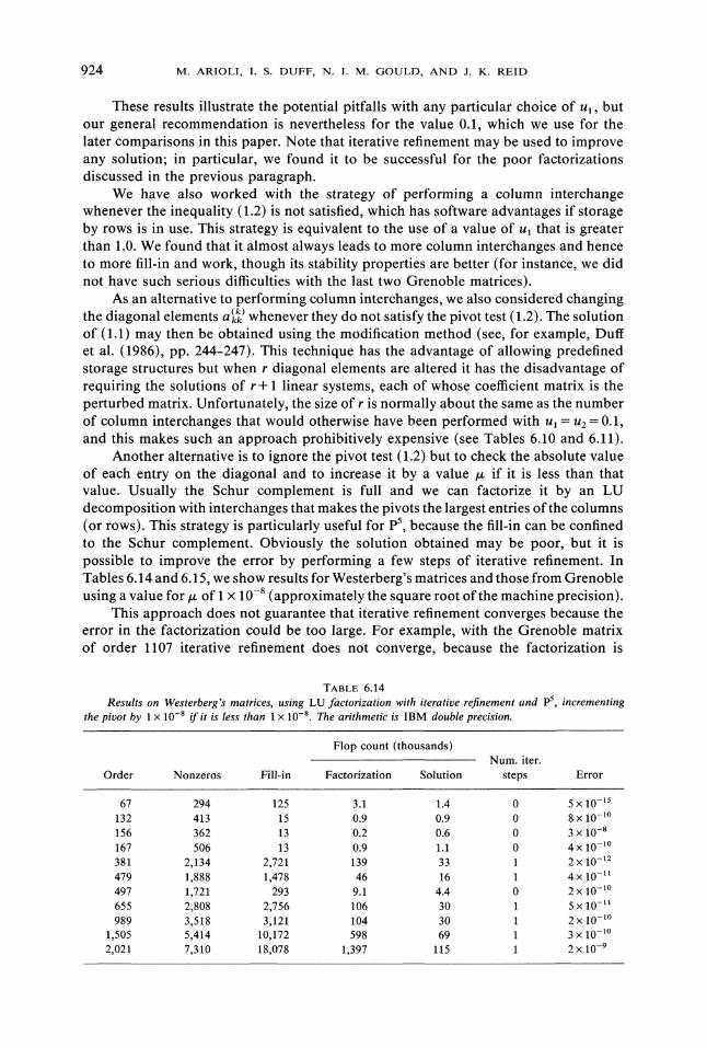
Another alternative is to ignore the pivot test (1.2) but to check the absolute valueof each entry on the diagonal and to increase it by a value /z if it is less than thatvalue. Usually the Schur complement is full and we can factorize it by an LUdecomposition with interchanges that makes the pivots the largest entries ofthe columns(or rows). This strategy is particularly useful for pS, because the fill-in can be confinedto the Schur complement. Obviously the solution obtained may be poor, but it ispossible to improve the error by performing a few steps of iterative refinement. InTables 6.14 and 6.15, we show results for Westerberg’s matrices and those from Grenobleusing a value for/ of I x 10-8 (approximately the square root ofthe machine precision).

This approach does not guarantee that iterative refinement converges because theerror in the factorization could be too large. For example, with the Grenoble matrixof order 1107 iterative refinement does not converge, because the factorization is

TABLE 6.14Results on Westerberg’s matrices, using LU factorization with iterative refinement and pS, incrementing

the pivot by 10-8 if it is less than x 10-8. The arithmetic is IBM double precision.

Flop count (thousands)Num. iter.

Order Nonzeros Fill-in Factorization Solution steps Error

67 294 125 3.1 1.4 0 5 x 10-15

132 413 15 0.9 0.9 0 8 x 10-1

156 362 13 0.2 0.6 0 3 10-8

167 506 13 0.9 1.1 0 4 x 10-1

381 2,134 2,721 139 33 2 x 10-12

479 1,888 1,478 46 16 4 x 10-11

497 1,721 293 9.1 4.4 0 2 x 10-655 2,808 2,756 106 30 5 10-989 3,518 3,121 104 30 2 10-1,505 5,414 10,172 598 69 3 10-1

2,021 7,310 18,078 1,397 115 2 10-9


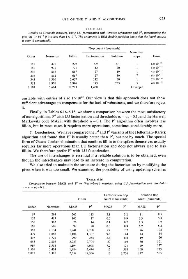
TABLE 6.15Results on Grenoble matrices, using LU factorization with iterative refinement and pS, incrementing the

pivot by 10-8 if it is less than x 10-8. The arithmetic is IBM double precision (note that the fourth matrix

is very ill-conditiond).

Flop count (thousands)Num. iter.

Order Nonzeros Fill-in Factorization Solution steps Error

115 421 222 6.9 6.1 8 10-16

185 975 771 42 20 5 x 10-13

216 812 617 27 19 4 10-17

216 812 617 27 80 7 6 10-2

343 1,310 2,657 132 50 2 10-16

512 1,976 2,996 193 265 5 4 10-13

1,107 5,664 12,723 1,458 Diverged

unstable with entries of size 1 1033. Our view is that this approach does not showsufficient advantages to compensate for the lack of robustness, and we therefore rejectit.

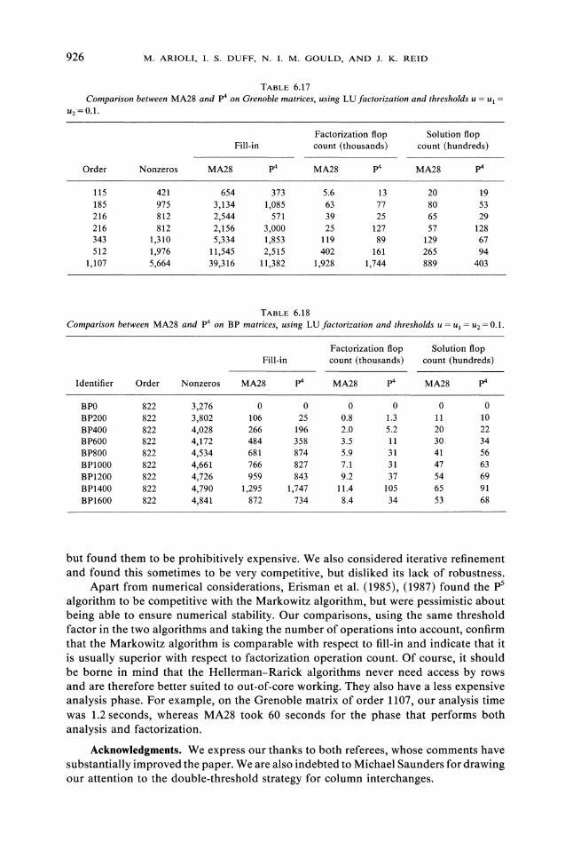
Finally, in Tables 6.16-6.18, we show a comparison between the most satisfactoryof our algorithms, p4 with LU factorization and thresholds ul u2 0.1, and the HarwellMarkowitz code MA28, with threshold u =0.1. The p4 algorithm often involves lessfill-in, but in most cases it requires more operations, sometimes considerably more.

7. Conclusions. We have compared the p4 and p5 variants ofthe Hellerman-Rarickalgorithm and found that p4 is usually better than pS, but not by much. The specialform of Gauss-Jordan elimination that confines fill-in to the spikes themselves usuallyrequires far more operations than LU factorization and does not always lead to lessfill-in. We therefore prefer p4 with LU factorization.

The use of interchanges is essential if a reliable solution is to be obtained, eventhough the interchanges may lead to an increase in computation.

We also tried to maintain the structure during the factorization by modifying thepivot when it was too small. We examined the possibility of using updating schemes

TABLE 6.16Comparison between MA28 and p4 on Westerberg’s matrices, using LU factorization and thresholds

U U U2--- 0.1.

Factorization flop Solution flopFill-in count (thousands) count (hundreds)

Order Nonzeros MA28 p4 MA28 p4 MA28 p4

67 294 267 113 2.1 3.2 11 8.5132 413 105 17 0.5 0.9 6.3 5.3156 362 26 14 0.1 0.2 1.5 1.2167 506 97 20 0.5 0.9 6.2 5.4381 2,134 1,941 2,708 25 137 76 102479 1,888 1,104 1,307 9.8 44 44 54497 1,721 299 254 2.4 8.0 19 20655 2,808 2,223 2,704 22 119 80 101989 3,518 1,194 4,098 7.2 171 69 137

1,505 5,414 1,984 7,474 12 368 109 2332,021 7,310 2,659 19,506 16 1,756 147 505


TABLE 6.17Comparison between MA28 and p4 on Grenoble matrices, using LU factorization and thresholds u u

u2 0.1.

Factorization flop Solution flopFill-in count (thousands) count (hundreds)

Order Nonzeros MA28 p4 MA28 p4 MA28 p4

115 421 654 373 5.6 13 20 19185 975 3,134 1,085 63 77 80 53216 812 2,544 571 39 25 65 29216 812 2,156 3,000 25 127 57 128343 1,310 5,334 1,853 119 89 129 67512 1,976 11,545 2,515 402 161 265 94

1,107 5,664 39,316 11,382 1,928 1,744 889 403

TABLE 6.18Comparison between MA28 and p4 on BP matrices, using LU factorization and thresholds u ul u 0.1.

Fill-inFactorization flopcount (thousands)

Solution flopcount (hundreds)

Identifier Order Nonzeros MA28 p4 MA28 p4 MA28 p4

BP0 822 3,276 0 0 0 0 0 0BP200 822 3,802 106 25 0.8 1.3 11 10BP400 822 4,028 266 196 2.0 5.2 20 22BP600 822 4,172 484 358 3.5 11 30 34BP800 822 4,534 681 874 5.9 31 41 56BP1000 822 4,661 766 827 7.1 31 47 63BP1200 822 4,726 959 843 9.2 37 54 69BP1400 822 4,790 1,295 1,747 11.4 105 65 91BP1600 822 4,841 872 734 8.4 34 53 68

but found them to be prohibitively expensive. We also considered iterative refinementand found this sometimes to be very competitive, but disliked its lack of robustness.

Apart from numerical considerations, Erisman et al. (1985), (1987) found the p5algorithm to be competitive with the Markowitz algorithm, but were pessimistic aboutbeing able to ensure numerical stability. Our comparisons, using the same thresholdfactor in the two algorithms and taking the number of operations into account, confirmthat the Markowitz algorithm is comparable with respect to fill-in and indicate that itis usually superior with respect to factorization operation count. Of course, it shouldbe borne in mind that the Hellerman-Rarick algorithms never need access by rowsand are therefore better suited to out-of-core working. They also have a less expensiveanalysis phase. For example, on the Grenoble matrix of order 1107, our analysis timewas 1.2 seconds, whereas MA28 took 60 seconds for the phase that performs bothanalysis and factorization.

Acknowledgments. We express our thanks to both referees, whose comments havesubstantially improved the paper. We are also indebted to Michael Saunders for drawingour attention to the double-threshold strategy for column interchanges.


REFERENCES

F. CACHARD (1981), Logiciel numerique associ# fi une modelisation de systmes informatiques, Thse,Universit6 Scientifique et M6dicale de Grenoble, et l’Institut National Polytechnique de Grenoble,Grenoble, France.

I. S. DUFF (1977), MA28A set ofFortran subroutinesfor sparse unsymmetric linear equations, Report AERER8730, Her Majesty’s Stationery Office, London, United Kingdom.

I. S. DUFF AND J. K. REID (1979), Some designfeatures ofa sparse matrix code, ACM Trans. Math. Software,5, pp. 18-35.

I. S. DUFF, A. M. ERISMAN, AND J. K. REID (1986), Direct Methodsfor Sparse Matrices, Oxford UniversityPress, London.

I. S. DUFF, R. G. GRIMES, AND J. G. LEWIS (1987), Sparse matrix test problems, ACM Trans. Math.Software, 15, pp. 1-14.

A. M. ERISMAN, R. G. GRIMES, J. G. LEWIS, AND W. G. POOLE, JR. (1985), A structurally stable modificationof Hellerman-Rarick’s p4 algorithm for reordering unsymmetric sparse matrices, SIAM J. Numer. Anal.,22, pp. 369-385.

A. M. ERISMAN, R. G. GRIMES, J. G. LEWIS, W. G. POOLE, JR., AND H. D. SIMON (1987), Evaluation

of orderings for unsymmetric sparse matrices, SIAM J. Sci. Statist. Comput., 8, pp. 600-624.A. GEORGE (1974), On block elimination for sparse linear systems, SIAM J. Numer. Anal., 11, pp. 585-603.E. HELLERMAN AND D. C. RARICK (1971), Reinversion with the preassigned pivot procedure, Math.

Programming, 1, pp. 195-216.(1972), The partitioned preassigned pivot procedure (p4), in Sparse Matrices and Their Applications,

D. J. Rose and R. A. Willoughby, eds., Plenum Press, New York, pp. 67-76.H. M. MARKOWITZ (1957), The elimination form of the inverse and its application to linear programming,

Management Sci., 3, pp. 255-269.M. A. SAUNDERS (1976), A fast, stable implementation of the simplex method using Bartels-Golub updating,

in Sparse Matrix Computations, Bunch and Rose, eds., Academic Press, New York, pp. 213-226.

Documents

THE FACTORIZATION MATRICES* - numerical.rl.ac.uk · Therefore, if Gauss-Jordan elimination is performed by applying ... is formed naturally when LUor Gauss-Jordan factorization is