Extended finite element methodsfor interface problems

Lecture notes (summer semester 2015)

Christoph Lehrenfeld

TU Wien

Last update: June 4, 2015

Abstract

We discuss numerical problems and solution methods for interface problems, mostlystemming from two-phase flow problems. The mathematical models of the consideredproblems describe rather standard continuum models on subdomains which are coupledthrough interface conditions. These conditions lead to (weak) discontinuities in thesolution quantities which makes the numerical treatment challenging.

For the description of the interface position and its evolution we consider interfacecapturing methods, for instance the level set method. In those methods the mesh is notaligned to the evolving interface such that the interface intersects mesh elements. Hence,the (possibly moving) discontinuities are located within individual elements which makesthe numerical treatment challenging.

For the discretization of such problems we present and analyze modern discretizationtechniques. The first component is an enrichment with an extended finite element(XFEM) space which provides the possibility to approximate discontinuous quantitiesaccurately without the need for aligned meshes. This enrichment, however, does notrespect all interface conditions automatically. To cure this issue we introduce anddiscuss different strategies to impose the interface condition using the discrete variationalformulation of the finite element method. For a stationary interface the combinationof both techniques offers a good way to provide reliable methods for the simulationof mass transport in two-phase flows. However, the most difficult aspect of two-phaseflow problems is the fact that the interface is typically not stationary, but moving intime. The numerical treatment of the moving discontinuity requires special care. Forthis purpose a space-time variational formulation is introduced and combined with thepreviously discussed techniques.

In this lecture we present the components and the resulting methods one after another,for stationary and non-stationary interfaces. We analyze the methods with respect toaccuracy and stability and discuss important properties.

The lecture is (to a great extend) based on [GR11, Leh15b].

2

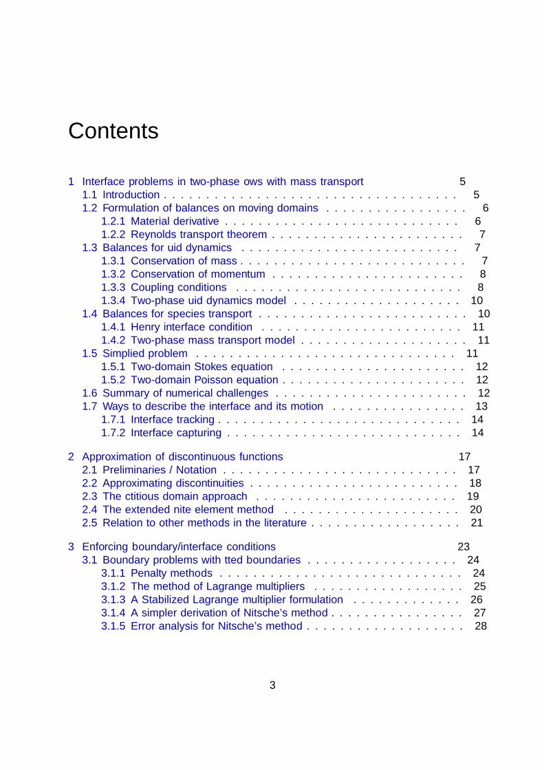
Contents

1 Interface problems in two-phase flows with mass transport 51.1 Introduction . . . . . . . . . . . . . . . . . . . . . . . . . . . . . . . . . . . 51.2 Formulation of balances on moving domains . . . . . . . . . . . . . . . . . 6

1.2.1 Material derivative . . . . . . . . . . . . . . . . . . . . . . . . . . . . 61.2.2 Reynolds transport theorem . . . . . . . . . . . . . . . . . . . . . . . 7

1.3 Balances for fluid dynamics . . . . . . . . . . . . . . . . . . . . . . . . . . 71.3.1 Conservation of mass . . . . . . . . . . . . . . . . . . . . . . . . . . . 71.3.2 Conservation of momentum . . . . . . . . . . . . . . . . . . . . . . . 81.3.3 Coupling conditions . . . . . . . . . . . . . . . . . . . . . . . . . . . 81.3.4 Two-phase fluid dynamics model . . . . . . . . . . . . . . . . . . . . 10

1.4 Balances for species transport . . . . . . . . . . . . . . . . . . . . . . . . . 101.4.1 Henry interface condition . . . . . . . . . . . . . . . . . . . . . . . . 111.4.2 Two-phase mass transport model . . . . . . . . . . . . . . . . . . . . 11

1.5 Simplified problem . . . . . . . . . . . . . . . . . . . . . . . . . . . . . . . 111.5.1 Two-domain Stokes equation . . . . . . . . . . . . . . . . . . . . . . 121.5.2 Two-domain Poisson equation . . . . . . . . . . . . . . . . . . . . . . 12

1.6 Summary of numerical challenges . . . . . . . . . . . . . . . . . . . . . . . 121.7 Ways to describe the interface and its motion . . . . . . . . . . . . . . . . 13

1.7.1 Interface tracking . . . . . . . . . . . . . . . . . . . . . . . . . . . . . 141.7.2 Interface capturing . . . . . . . . . . . . . . . . . . . . . . . . . . . . 14

2 Approximation of discontinuous functions 172.1 Preliminaries / Notation . . . . . . . . . . . . . . . . . . . . . . . . . . . . 172.2 Approximating discontinuities . . . . . . . . . . . . . . . . . . . . . . . . . 182.3 The fictitious domain approach . . . . . . . . . . . . . . . . . . . . . . . . 192.4 The extended finite element method . . . . . . . . . . . . . . . . . . . . . 202.5 Relation to other methods in the literature . . . . . . . . . . . . . . . . . . 21

3 Enforcing boundary/interface conditions 233.1 Boundary problems with fitted boundaries . . . . . . . . . . . . . . . . . . 24

3.1.1 Penalty methods . . . . . . . . . . . . . . . . . . . . . . . . . . . . . 243.1.2 The method of Lagrange multipliers . . . . . . . . . . . . . . . . . . 253.1.3 A Stabilized Lagrange multiplier formulation . . . . . . . . . . . . . 263.1.4 A simpler derivation of Nitsche’s method . . . . . . . . . . . . . . . . 273.1.5 Error analysis for Nitsche’s method . . . . . . . . . . . . . . . . . . . 28

3

3.2 Interface problems with fitted interfaces . . . . . . . . . . . . . . . . . . . 313.2.1 Stabilized Lagrange multipliers → Interior Penalty methods . . . . . 323.2.2 Connections to other methods . . . . . . . . . . . . . . . . . . . . . . 33

3.3 Interface problems with unfitted interfaces . . . . . . . . . . . . . . . . . . 343.3.1 The Nitsche method for unfitted interface problems . . . . . . . . . . 343.3.2 Weighted average and the choice of λ . . . . . . . . . . . . . . . . . . 363.3.3 Error analysis for Nitsche-XFEM (diffusion dominates) . . . . . . . . 37

3.4 Boundary problems on unfitted domains . . . . . . . . . . . . . . . . . . . 463.4.1 The Nitsche formulation . . . . . . . . . . . . . . . . . . . . . . . . . 473.4.2 Ghost penalty . . . . . . . . . . . . . . . . . . . . . . . . . . . . . . 47

3.5 Preconditioning of linear systems . . . . . . . . . . . . . . . . . . . . . . . 503.5.1 Basis transformation (β → 1) . . . . . . . . . . . . . . . . . . . . . . 513.5.2 Observations for simple preconditioners . . . . . . . . . . . . . . . . 523.5.3 Preconditioning strategies . . . . . . . . . . . . . . . . . . . . . . . . 543.5.4 Parameter dependencies for the sliver test case . . . . . . . . . . . . 59

4 Representation of the interface and its motion 614.1 Interface tracking methods . . . . . . . . . . . . . . . . . . . . . . . . . . . 614.2 The Volume of Fluid method . . . . . . . . . . . . . . . . . . . . . . . . . 624.3 The level set method . . . . . . . . . . . . . . . . . . . . . . . . . . . . . . 634.4 Phase field representation . . . . . . . . . . . . . . . . . . . . . . . . . . . 65

5 Space-Time finite element methods for problems with moving interfaces 665.1 Problem description . . . . . . . . . . . . . . . . . . . . . . . . . . . . . . 66

5.1.1 Solution strategies . . . . . . . . . . . . . . . . . . . . . . . . . . . . 665.2 Space-time DG formulation for a parabolic model problem . . . . . . . . . 715.3 Space-time extended finite elements . . . . . . . . . . . . . . . . . . . . . . 745.4 Nitsche formulation for interface conditions in space-time . . . . . . . . . . 75

5.4.1 Derivation of the method . . . . . . . . . . . . . . . . . . . . . . . . 76

A Exercise solutions 80

B Brezzi’s Theorem 84

4

1 Interface problems in two-phaseflows with mass transport

1.1 Introduction

The two-phase flow problem (including additional transport problems) will be our guidingexample of interface problems. In this chapter we derive two-phase flow models for thefluid dynamic and the mass transport and discuss the arising numerical challenges. Atthe end of the chapter we give a brief structure of the remaining parts of the lecture.

Lagrangian and Eulerian descriptions In fluid dynamics a specification of the balancelaws which is based on specific fixed locations in space is called Eulerian. The counter-part of an Eulerian description is the Lagrangian specification where the balances areformulated relative to a fluid parcel which moves through space and time following theflow field.

We derive an Eulerian description of the balance laws in two-phase flows in a sharpinterface formulation. The fluids are contained in an open domain Ω ⊂ Rd, d ∈ 1, 2, 3.The fluids are contained in the domains Ω1, Ω2 which are separated by Γ = Ω1 ∩ Ω2.We assume that one phase is completely surrounded by the other, s.t. Γ ∩ ∂Ω = ∅ (∀ t ).

Γ

Ω1

Ω2

Γ

Ω1

Ω2

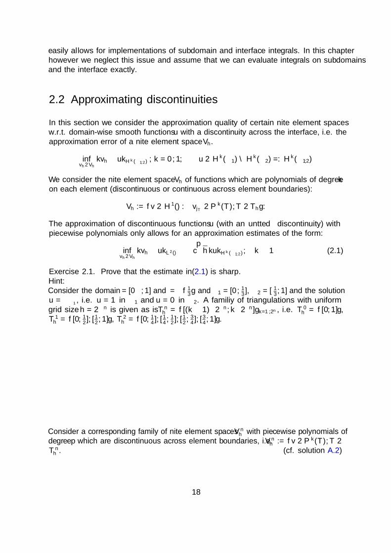
Figure 1.1.1: Sketch of two phases.

5

Assumptions on the two-phase flow equations

We make the following assumptions:

• The fluids are immiscible (pure, no mixtures) and there is no phase transition.

• The interface has thickness zero, we say the interface is sharp.

• The fluids are incompressible.

• The fluids are viscous and Newtonian.

• We consider isothermal conditions, that implies that there are no variations indensity or (dynamic) viscosity due to temperature.

• Transported species do not adhere at the interface and no chemical reactions takeplace at the interface.

1.2 Formulation of balances on moving domains

1.2.1 Material derivative

Let Xξ(t) denote the solution to

Xξ(t) = u(Xξ(t), t), t > 0, Xξ(0) = ξ

for a point ξ ∈ Ω, called the trajectory of the particle with initial position ξ.

The material derivative of a (sufficiently smooth) function f(x, t) is defined as the rateof change of f w.r.t. to the trajectory crossing x in t:

f(Xξ(t), t) =d

dtf(Xξ(t), t) =

∂

∂tf +

∂Xξ

∂t· ∇f

where in the last step we have to assume that f is also sufficiently smooth in a neighbor-hood of x.

Due to the immiscibility of the fluids we have that Xξ(t) ∈ Ωi(t) ∀ t for a fixed i = 1 ori = 2, i.e. a particle will not change phase. As a consequence particles on the interfacewill stay on the interface and thus

Γ(t) = Xξ(t) : ξ ∈ Γ(0).

For u = 0 on ∂Ω, there also holds Ωi(t) = Xξ(t) : ξ ∈ Ωi(0).Another direct conclusion concerns the velocity of the interface V .

V · nΓ = u · nΓ,

with nΓ the normal to the interface pointing from Ω1 to Ω2.

6

1.2.2 Reynolds transport theorem

Consider a (small) subdomain W0 ⊂ Ω which is completely contained in one phase, i.e.W0 ∈ Ωi(0), i ∈ 1, 2, called a material volume. We define the material volume at alater time as

W (t) := Xξ(t) : ξ ∈ W0.

x

t

W (t)

W (0) = W0

Figure 1.2.1: Sketch of material volume.

The rate of change of a smooth quantity f in a (time-dependent) domain W (t)can be described as

d

dt

∫W (t)

f(x, t)dx =

∫W (t)

f(x, t) + f div(u(x, t)) dx

=

∫W (t)

∂

∂tf(x, t) + div(f · u)(x, t) dx

=

∫W (t)

∂

∂tf(x, t) dx +

∫∂W (t)

f(u · n)(s, t) ds

Theorem 1.1 (Reynold’s transport theorem).

1.3 Balances for fluid dynamics

1.3.1 Conservation of mass

The total mass within the material volume is conserved (no ingoing or outgoing fluxes,no sources), this implies

d

dt

∫W (t)

ρ dx︸ ︷︷ ︸total mass in W (t)

=

∫W (t)

∂ρ

∂t+ div(ρu) dx = 0.

7

As the material volume W0 and the time t are essentially arbitrary, the balance can belocalized towards

∂ρ

∂t+ div(ρu) = 0 in Ωi(t).

Now, further exploiting ρ = const within each phase gives

div(u) = 0 in Ωi(t). (1.1)

1.3.2 Conservation of momentum

Following Newton’s law the rate of change of the momentum within the control volumehas to balance with the forces acting on that volume:

d

dt

∫W (t)

ρu dx︸ ︷︷ ︸total momentum W (t)

=

∫W (t)

ρg dx +

∫∂W (t)

σ · n ds︸ ︷︷ ︸forces acting on W (t)

=

∫W (t)

ρg + div(σ)dx.

This gives ∫W (t)

∂(ρu)

∂t+ div(ρu⊗ u)− div(σ)dx =

∫W (t)

ρg dx

Due to ρ = const (and hence (1.1)) we have div(ρu⊗ u) = ρ(u · ∇)u. Further we usethe assumed Newtonian behavior of the stress tensor, i.e.

σ = −pI + λ(div(u))︸ ︷︷ ︸=0

I + µD(u), D(u) = ∇u +∇uT

All together, the localized versions give the Navier-Stokes equations for the subdo-mains:

ρ(∂u∂t

+ (u · ∇)u) +∇p− div(µD(u)) = ρg in Ωi(t), i = 1, 2div(u) = 0 in Ωi(t), i = 1, 2.

(1.2)

Now, we are only missing the boundary conditions and the coupling conditions at theinterface to complete the model for the two-phase hydrodynamics.

1.3.3 Coupling conditions

To close the model in (1.2) w.r.t. to the interface conditions we need 2d scalar conditions,with d the space dimension.

8

Continuity As there is no change in phase and the fluids are viscous, we conclude thatthe velocity is continuous, i.e.

[[u]] = 0 on Γ(t)

with the jump operator [[f ]] = limh→0 f(x− hnΓ)− f(x + hnΓ) for sufficiently smoothfunctions f . These are the first d conditions. The d remaining scalar conditons are relatedto the force balance at the interface. Note that due to div(u) = 0 in Ωi(t), i = 1, 2 and[[u · nΓ]] = 0 on Γi(t), we have div(u) = 0 in Ω (in the L2-sense).

Surface tension force We now consider a control volume W (t) which contains bothphases (and a part of the interface). We have W1(t) := W (t)∩Ω1(t), W2(t) := W (t)∩Ω2(t)and ΓW (t) := W (t)∩Γ(t). At the interface an additional force exists, the surface tensionforce. It is usually modeled as

−τ∫

ΓW (t)

κ · nΓ ds

with a constant surface tension coefficient τ and the mean curvature κ (κ(x) = div(nΓ(x))).In the definition of the curvature the orientation can be different in other literature, inour definition a convex interior of Γ results in a negative κ. The curvature of a sphere(in d dimensions) with radius R is κ = d−1

R.

A force balance on W (t) gives

d

dt

∫W (t)

ρu dx︸ ︷︷ ︸rate of change in mom.

=

∫W (t)

ρg dx︸ ︷︷ ︸volume force

+

∫∂W (t)

σ · n ds︸ ︷︷ ︸surface force(stress)

− τ∫

ΓW

κ · nΓ ds︸ ︷︷ ︸surface tension force

In order to do partial integration on the stress tensor part of the outer forces we have todivide the integral into its subdomains (where σ is smooth).∫

∂W (t)

σ · n =

∫∂W1(t)

σ1 · n1 ds +

∫∂W2(t)

σ2 · n2 ds−∫

ΓW

(σ1 · n1 + σ2 · n2) ds

and hence get∫W (t)

ρ(∂

∂tu + (u · ∇)u) +∇p− div(µD(u)) dx =

∫W (t)

ρg −∫

ΓW

[[σ · nΓ]] + τκnΓ ds

Note that the balance holds already for W1(t) and W2(t) and we can thus concludethat there holds

∫ΓW

[[σ · nΓ]] ds = −τ∫

ΓWκnΓ ds and localizing this (ΓW is essentially

arbitrary) we get:[[σ · nΓ]] = −τκnΓ on Γ(t) (1.3)

9

1.3.4 Two-phase fluid dynamics model

We end up with the a standard model from the literature [Scr60, BKZ92, GR11].

Given suitable boundary conditions and initial values for u, find u(x, t) and p(x, t),s.t.

ρi(∂

∂tu + (u · ∇)u)− div(µiD(u)) +∇p = ρig in Ωi(t), i = 1, 2 (1.4a)

div(u) = 0 in Ωi(t), i = 1, 2, (1.4b)

[[σ · nΓ]] = −τκnΓ, on Γ(t), (1.4c)

[[u]] = 0, on Γ(t). (1.4d)

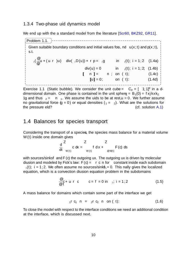
Problem 1.1.

Exercise 1.1 (Static bubble). We consider the unit cube Ω = Cd = [−1, 1]d in a d-dimensional domain. One phase is contained in the unit sphere Ω1 = B1(0) = x| ‖x‖2 ≤1 and thus Ω2 = Ω \ Ω1. We assume the fluids to be at rest, u = 0. We further assumeno gravitational force (g = 0) or equal densities (ρ1 = ρ2). What are the solutions forthe pressure field? (cf. solution A.1)

1.4 Balances for species transport

Considering the transport of a species c, the species mass balance for a material volumeW (t) inside one domain gives

d

dt

∫W (t)

c dx =

∫W (t)

f dx +

∫∂W (t)

F (c) ds

with sources/sinks f and F (c) the outgoing flux. The outgoing flux is driven by moleculardiffusion and modeled by Fick’s law: F (c) = α∇c ·n for α constant inside each subdomainΩi(t), i = 1, 2. We often assume no sources/sinks, f = 0. This finally gives the localizedequation, which is a convection diffusion equation problem in the subdomains

∂

∂tc+ u · ∇c− α∆c = f = 0 in Ωi, i = 1, 2 (1.5)

A mass balance for domains which contain some part of the interface we get

α1∇c1 · nΓ = α2∇c2 · nΓ on Γ(t). (1.6)

To close the model with respect to the interface conditions we need an additional conditionat the interface, which is discussed next.

10

1.4.1 Henry interface condition

The second interface condition is the Henry interface condition, that results from aconstitutive law known as Henry’s law. Henry’s law assumes that chemical potentialsfrom both sites are in balance, i.e. an instantaneous thermodynamical equilibrium isassumed. This assumption is reasonable as long as kinetic processes at the interface aresufficiently fast. Then, Henry’s law states that the concentrations at the interface areproportional to the partial pressure of the species in the fluids p = βici with constantsβi which depend on the solute, the solvent and the temperature. Using these constantsHenry’s law reads as

β1c1 = β2c2.

For further details on the modeling we refer to [Ish75, SAC97, SSO07]. The Henryinterface condition leads to a discontinuity of the quantity c across the (evolving) interfaceas we typically have β1 6= β2.

1.4.2 Two-phase mass transport model

Given suitable initial and boundary conditions for c, find c(x, t), s.t.

∂

∂tc+ u · ∇c− div(α∇c) = f in Ωi(t), i = 1, 2, (1.7a)

[[α∇c · n]] = 0 on Γ, (1.7b)

[[βc]] = 0 on Γ, (1.7c)

Problem 1.2.

1.5 Simplified problem

We introduce two simplified problems which are stationary versions of problem 1.1 andproblem 1.2 (with ∂tu = 0) which further neglect convection effects.

11

1.5.1 Two-domain Stokes equation

Given suitable boundary conditions for u, find u(x) and p(x), s.t.

− div(µiD(u)) +∇p = ρig in Ωi, i = 1, 2

div(u) = 0 in Ωi, i = 1, 2,

[[σ · nΓ]] = −τκnΓ, [[u]] = 0, on Γ.

Problem 1.3.

There holds div(D(u)) = ∆u + ∇ div(u), s.t. one often replaces − div(µiD(u)) with− div(µi∇u). Note however, that the treatment of the interface and boundary conditionsis most natural for a formulation with − div(µiD(u)).

1.5.2 Two-domain Poisson equation

The simplest version of problem 1.2 is obtained by considering a stationary problemwithout convection:

Given suitable boundary conditions for c, find c(x), s.t.

− div(α∇c) = f in Ωi, i = 1, 2, (1.9a)

[[α∇c · n]] = 0 on Γ, (1.9b)

[[βc]] = 0 on Γ, (1.9c)

c = gD on ∂Ω. (1.9d)

Problem 1.4.

For β1 = β2 (or after reformulation as a problem of βc) the problem is a standard problemin the literature of interface problems.

1.6 Summary of numerical challenges

We briefly summarize the most important features of the derived models:

• Solutions to the fluid dynamics problem may exhibit discontinuities across theinterface, i.e. the velocity may have kinks (”weak discontinuity”) while the pressure(and the species concentration) may have jumps (”strong discontinuity”).

• The surface tension force acts only on a manifold and is sensitive to geometricalerrors. An accurate numerical treatment is challenging.

• The (weak) discontinuities travel in time (following the interface).

12

• In the scope of this lecture we focus on methods where the interface is ”captured”which means that only an implicit description of the interface exists, s.t. theinterface is typically not aligned to the computational mesh.

Other problems with interfaces

There are many other fluid flow problems which involve (moving) interfaces or boundaries.In the student projects of this lecture some of these problems can be considered, e.g.:

• Free surface flows, i.e. one-phase flows with moving boundaries.

• Surfactant equations: In many two-phase flows soluable species adhere at theinterface. The distribution of these quantities on the interface is a challenging taskfor the numerical discretization.

• Osmosis problems: Here, the concentration at the interface while the mean curvatureof the domain boundary determine the evolution of the domain.

• Phase transition due to melting (Stefan problem). The problem is formulated forthe temperature of water/ice and the interface is implicitly defined as the zero-levelof the temperature.

• . . .

1.7 Ways to describe the interface and its motion

In the description of physical balances a specification of the laws can be set in differentcoordinate systems. For fluid dynamic problems the two most important ones are an“Eulerian” and a “Lagrangian” coordinate system. Both (and mixed) formulations are usedto derive different discretization methods for flow problems. Discretizations based on aLagrangian description offer a natural treatment for problems with moving boundaries orinterfaces. However, Lagrangian methods have significant drawbacks if deformations getlarge or topologies change. These issues can be overcome by Eulerian methods. However,the discretization of problems with moving boundaries or interfaces in an Eulerian frameis difficult. A major component of the numerical difficulties discussed in this lecture arisefrom the fact that we consider the problem in an Eulerian framework with an implicitdescription of the interface. In contrast to methods which are based on a Lagrangianformulation at the interface, e.g. a full Lagrangian method or an Arbitrary-Lagrangian-Eulerian formulation, the computational mesh is not adapted to fit the interface. As aconsequence the interface and thus the discontinuity of the concentration lies or evenmoves inside a computational element rather than coinciding with element facets.

13

There are also many intermediate ways between both descriptions, especially coordi-nate systems where only the moving boundary or interface is treated as a Lagrangianparticles.

For the representation of a possibly moving interface, there are two popular techniquesto represent the motion of a sharp interface. Most methods for sharp interface modelsof two-phase flows fall into one of those two classes: interface tracking or interfacecapturing methods. We only briefly mention the approaches here. In chapter 4 this topicis discussed in more detail.

1.7.1 Interface tracking

In interface tracking methods, points on the interface (grid points or artificial markerpoints) are transported explicitly with the flow field. This method has the advantagethat an explicit description of the interface can be preserved. The major drawback of thismethod is that the distribution of control points (grid points or marker points) at theinterface will typically deviate significantly from a uniform distribution and redistributiongets necessary. If grid points of a mesh are used as control points, this means thatan automated remeshing procedure has to take place after several time steps whichis typically challenging and computationally expensive. Especially difficult to handleare situations where the topology of the domains changes, for instance collisions ofdroplets.

1.7.2 Interface capturing

Interface capturing methods such as the Volume of Fluid (VoF) and the level set methodwere developed to circumvent problems with topology changes and frequent remeshing.These methods use an implicit description of the interface, typically in an Eulerianframework. For that an auxiliary indicator field is introduced. The transport of this fieldis described by a linear hyperbolic PDE. This topic is discussed in chapter 4.

In the following we will concentrate on the discussion of problems where an interfacecapturing method is used. This has the following important implications:

• The interface is described only implicitly via some characterization of the indicatorfield.

• The interface is not aligned with element boundaries.

14

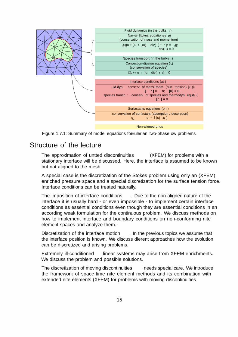
ΓΩ1

Ω2

Fluid dynamics (in the bulks Ωi)

Navier-Stokes equations (u, p)(conservation of mass and momentum)

ρi(∂tu + (u · ∇)u)− div(σ) +∇p = ρig,div(u) = 0

Species transport (in the bulks Ωi)

Convection-diffusion equation (c)(conservation of species)

∂tc+ (u · ∇)c− div(α∇c) = 0

Interface conditions (at Γ)

fluid dyn.: conserv. of mass+mom. (surf. tension) (u, p)[[σ · n]] = τκn, [[u]] = 0

species transp..: conserv. of species and thermodyn. equil. (c)[[βc]] = 0

Surfactants equations (on Γ)

conservation of surfactant (adsorption / desorption)cΓ − αΓ∆ΓcΓ = f(u|Γ, cΓ)

Non-aligned grids

Figure 1.7.1: Summary of model equations for Eulerian two-phase flow problems

Structure of the lecture

• The approximation of unfitted discontinuities (XFEM) for problems with astationary interface will be discussed. Here, the interface is assumed to be knownbut not aligned to the mesh

• A special case is the discretization of the Stokes problem using only an (XFEM)enriched pressure space and a special discretization for the surface tension force.Interface conditions can be treated naturally.

• The imposition of interface conditions. Due to the non-aligned nature of theinterface it is usually hard - or even impossible - to implement certain interfaceconditions as essential conditions even though they are essential conditions in anaccording weak formulation for the continuous problem. We discuss methods onhow to implement interface and boundary conditions on non-conforming finiteelement spaces and analyze them.

• Discretization of the interface motion. In the previous topics we assume thatthe interface position is known. We discuss different approaches how the evolutioncan be discretized and arising problems.

• Extremely ill-conditioned linear systems may arise from XFEM enrichments.We discuss the problem and possible solutions.

• The discretization of moving discontinuities needs special care. We introducethe framework of space-time finite element methods and its combination withextended finite elements (XFEM) for problems with moving discontinuities.

15

Excursion: The two-phase Stokesproblem

Weak formulation of two-phase Stokes problems The weak formulation for theStokes problem takes the following form:Find u ∈ [H1(Ω)]3, p ∈ L2(Ω), s.t.∫

Ω1,2

µi2D(u) : D(v) dx−

∫Ω1,2

div(u)q dx−∫

Ω1,2

div(v)p dx =

∫Ω1,2

ρigv dx−τ∫

Γ

κnΓv ds

for all v ∈ [H1(Ω)]3, q ∈ L2(Ω).Exercise 1.2 (Computational exercise, using tutorial mystokes). Follow the instructionsof the corresponding tutorials to solve the two-phase Stokes problem on a fitted mesh intwo and three dimensions. Investigate the following:

• The pressure is in general discontinuous due to the surface tension force. How welldo the different velocity-pressure spaces cope with this discontinuity?

• How sensitive is the solution to the approximation quality of the surface tensionforce?

One interesting feature of the two-phase Stokes problem is the fact, that interfaceconditions are imposed naturally on the finite element spaces for “standard” stable finiteelement methods for the Stokes problem. This especially means, that we do not have toimpose an additional condition at the interface.

16

2 Approximation of discontinuousfunctions

This chapter is devoted to the approximation of functions which have special discontinu-ities in the sense that the location of these are known.

2.1 Preliminaries / Notation

Let Thh>0 be a family of shape regular simplex triangulation of Ω. A triangulation Thconsists of simplices T , with hT := diam(T ) and h := maxhT | T ∈ Th. In general wehave that the interface Γ does not coincide with element boundaries. The triangulationis unfitted. We introduce some notation for cut elements, i.e. elements T with Γ ∩ T 6= ∅.For any simplex T ∈ Th, Ti := T ∩ Ωi denotes the part of T in Ωi and ΓT := T ∩ Γthe part of the interface that lies in T . T Γ

h denotes the set of elements that are “closeto the interface”, T Γ

h := T : T ∩ Γ 6= ∅. The corresponding domain is denoted byΩΓ = x ∈ T : T ∈ T Γ

h . Further, we define the set of elements with nonzero support inone domain: T ih := T : T ∩ Ωi 6= ∅, i = 1, 2, the corresponding domain is denoted byΩ+i = x ∈ T : T ∈ T ih. We also define the domain of uncut elements in domain i as

Ω−i = Ωi \ ΩΓ = Ω+i \ ΩΓ.

At some places we use the notation with the relations and .Definition 2.1 (Notation: smaller/greater up to a constant (, ), equivalent (')).For a, b ∈ R we use the notation a b (a b), if there exists a constant c ∈ R suchthat there holds a ≤ c b (a ≥ c b), with c independent of h or the cut position. If we havea b and b a, we write a ' b.Assumption 2.1 (Resolution of the interface). We assume that the resolution close tothe interface is sufficiently high such that the interface can be resolved by the triangulation,in the sense that if Γ∩T =: ΓT 6= ∅ then ΓT can be represented as the graph of a functionon a planar cross-section of T . We refer to [HH02] for precise conditions.Remark 2.1 (Interface approximation). In implementations of any method with anunfitted triangulation one needs to deal with the interface Γ in terms of subdomain andinterface integrals. In practice Γ is often defined implicitly, e.g. as the zero level of agiven level set function. As soon as the level set function is not (piecewise) linear theinterface Γ is not (piecewise) planar and an explicit construction is (usually) not feasible.Often an approximation Γh of Γ is constructed which has an explicit representation and

17

easily allows for implementations of subdomain and interface integrals. In this chapterhowever we neglect this issue and assume that we can evaluate integrals on subdomainsand the interface exactly.

2.2 Approximating discontinuities

In this section we consider the approximation quality of certain finite element spacesw.r.t. domain-wise smooth functions u with a discontinuity across the interface, i.e. theapproximation error of a finite element space Vh.

infvh∈Vh

‖vh − u‖Hk(Ω1,2) , k = 0, 1, u ∈ Hk(Ω1) ∩Hk(Ω2) =: Hk(Ω1,2)

We consider the finite element space Vh of functions which are polynomials of degree kon each element (discontinuous or continuous across element boundaries):

Vh := v ∈ H1(Ω) : v|T ∈ Pk(T ), T ∈ Th.

The approximation of discontinuous functions u (with an unfitted discontinuity) withpiecewise polynomials only allows for an approximation estimates of the form:

infvh∈Vh

‖vh − u‖L2(Ω) ≤ c√h ‖u‖Hk(Ω1,2), k ≥ 1 (2.1)

Exercise 2.1. Prove that the estimate in (2.1) is sharp.Hint:Consider the domain Ω = [0, 1] and Γ = 1

3 and Ω1 = [0, 1

3], Ω2 = [1

3, 1] and the solution

u = χΩ1, i.e. u = 1 in Ω1 and u = 0 in Ω2. A familiy of triangulations with uniformgrid size h = 2−n is given as is T nh = [(k − 1) · 2−n, k · 2−n]k=1,2n, i.e. T 0

h = [0, 1],T 1h = [0, 1

2], [1

2, 1], T 2

h = [0, 14], [1

4, 1

2], [1

2, 3

4], [3

4, 1].

x

u Γ = 13

10

T 3h

T 2h

T 1h

Consider a corresponding family of finite element spaces V nh with piecewise polynomials of

degree p which are discontinuous across element boundaries, i.e. V nh := v ∈ Pk(T ), T ∈

T nh . (cf. solution A.2)

18

Consider the simpler problem with β1 = β2. The jump discontinuity vanishes but thediscontinuity in the derivative (kink discontinuity) due to different diffusivities α remains.In this case the approximation quality of standard finite element spaces is better. Still,the sub-optimal approximation error estimate

infvh∈Vh

‖vh − u‖L2(Ω) ≤ ch32 ‖u‖Hk(Ω1,2), k ≥ 2

is sharp, independent of the polynomial degree of the finite element space Vh. In thenext sections a remedy to this problem is presented.

2.3 The fictitious domain approach

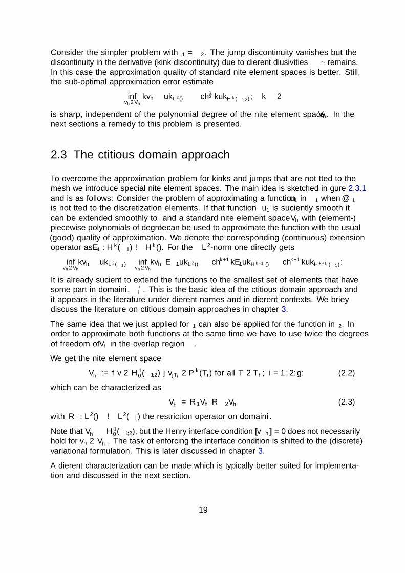
To overcome the approximation problem for kinks and jumps that are not fitted to themesh we introduce special finite element spaces. The main idea is sketched in figure 2.3.1and is as follows: Consider the problem of approximating a function u1 in Ω1 when ∂Ω1

is not fitted to the discretization elements. If that function u1 is sufficiently smooth itcan be extended smoothly to Ω and a standard finite element space Vh with (element-)piecewise polynomials of degree k can be used to approximate the function with the usual(good) quality of approximation. We denote the corresponding (continuous) extensionoperator as E1 : Hk(Ω1)→ Hk(Ω). For the L2-norm one directly gets

infvh∈Vh‖vh − u‖L2(Ω1)≤ inf

vh∈Vh‖vh − E1u‖L2(Ω)≤chk+1‖E1u‖Hk+1(Ω)≤chk+1‖u‖Hk+1(Ω1).

It is already sufficient to extend the functions to the smallest set of elements that havesome part in domain i, Ω+

i . This is the basic idea of the fictitious domain approach andit appears in the literature under different names and in different contexts. We brieflydiscuss the literature on fictitious domain approaches in chapter 3.

The same idea that we just applied for Ω1 can also be applied for the function in Ω2. Inorder to approximate both functions at the same time we have to use twice the degreesof freedom of Vh in the overlap region ΩΓ.

We get the finite element space

V Γh := v ∈ H1

0 (Ω1,2) | v|Ti ∈ Pk(Ti) for all T ∈ Th, i = 1, 2. . (2.2)

which can be characterized as

V Γh = R1Vh ⊕R2Vh (2.3)

with Ri : L2(Ω)→ L2(Ωi) the restriction operator on domain i.

Note that V Γh ⊂ H1

0 (Ω1,2), but the Henry interface condition [[βvh]] = 0 does not necessarilyhold for vh ∈ V Γ

h . The task of enforcing the interface condition is shifted to the (discrete)variational formulation. This is later discussed in chapter 3.

A different characterization can be made which is typically better suited for implementa-tion and discussed in the next section.

19

Ω+1

Ω+2

Γ

Ω−2

Ω−1

ΩΓ

Figure 2.3.1: Fictituous domain approach applied for domain Ω1 (left) and Ω2 (center). Com-bining both results in a finite element space with double-valued representatives inthe overlap region ΩΓ(right).

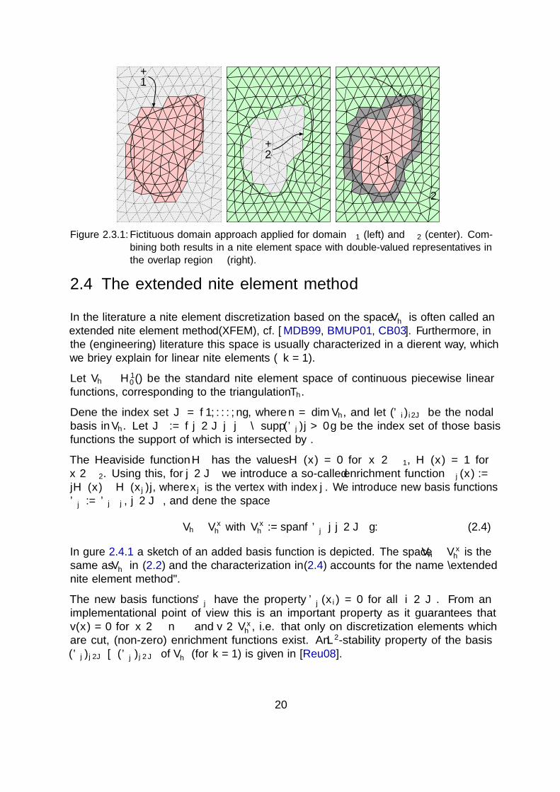
2.4 The extended finite element method

In the literature a finite element discretization based on the space V Γh is often called an

extended finite element method (XFEM), cf. [MDB99, BMUP01, CB03]. Furthermore, inthe (engineering) literature this space is usually characterized in a different way, whichwe briefly explain for linear finite elements (k = 1).

Let Vh ⊂ H10 (Ω) be the standard finite element space of continuous piecewise linear

functions, corresponding to the triangulation Th.Define the index set J = 1, . . . , n, where n = dimVh, and let (ϕi)i∈J be the nodalbasis in Vh. Let JΓ := j ∈ J | |Γ ∩ supp(ϕj)| > 0 be the index set of those basisfunctions the support of which is intersected by Γ.

The Heaviside function HΓ has the values HΓ(x) = 0 for x ∈ Ω1, HΓ(x) = 1 forx ∈ Ω2. Using this, for j ∈ JΓ we introduce a so-called enrichment function Φj(x) :=|HΓ(x)−HΓ(xj)|, where xj is the vertex with index j. We introduce new basis functionsϕΓj := ϕjΦj, j ∈ JΓ, and define the space

Vh ⊕ V xh with V x

h := spanϕΓj | j ∈ JΓ . (2.4)

In figure 2.4.1 a sketch of an added basis function is depicted. The space Vh ⊕ V xh is the

same as V Γh in (2.2) and the characterization in (2.4) accounts for the name “extended

finite element method”.

The new basis functions ϕΓj have the property ϕΓ

j (xi) = 0 for all i ∈ J . From animplementational point of view this is an important property as it guarantees thatv(x) = 0 for x ∈ Ω \ ΩΓ and v ∈ V x

h , i.e. that only on discretization elements whichare cut, (non-zero) enrichment functions exist. An L2-stability property of the basis(ϕj)j∈J ∪ (ϕΓ

j )j∈JΓof V Γ

h (for k = 1) is given in [Reu08].

20

Figure 2.4.1: Example of an XFEM shape functions. On the left a shape function ϕj from thestandard finite element space Vh is shown. On the right the restriction R1ϕj onΩ1 is shown. The function R1ϕj is a basis function of V x

h .

In the XFEM literature the enrichment process is typically characterized more general.The presented enrichment technique is a special case, called the “Heaviside” enrich-ment.

2.5 Relation to other methods in the literature

The general idea of fictitious domain approaches is to find a solution to a PDE problemon a complicated domain Ω by replacing the problem with a problem on a larger domainΩ ⊃ Ω such that the restriction to Ω of the solution coincides with the solution ofthe original problem. Typically, the domain Ω is chosen as a simple geometry whichis easily meshed. The main motivation for this approach is that one can work with asimple background mesh that is independent of a (possibly) complex and time-dependentgeometry. This apparent simplification comes at a price. The interface is not aligned toelement boundaries of a triangulation, the interface is unfitted. Managing data structurespertaining the actual geometry is in general not trivial.

The first unfitted finite element methods have been investigated and analyzed in, a.o.,[Bab73b, BE86, GPP94a, GPP94b, GG95]. An important problem for unfitted finiteelements is the question of how to implement boundary(interface) conditions. This isdue to the fact that it is not feasible to implement Dirichlet (or continuity) conditionsas essential boundary conditions into the unfitted finite element space. The mentionedpapers use penalty or Lagrange multiplier techniques to enforce the desired boundary(interface) conditions. The problem of enforcing boundary (interface) conditions will bediscussed in chapter 3.

The general idea of the fictitious domain method is applied in many different contextsunder different names. We mention a few of these methods.

In fluid-structure interaction problems, immersed boundary (IB) methods (see, e.g.,[PM89]) use non-matching overlapping grids, for example a static mesh for the fluid

21

and a moving mesh for the object which is in contact with the fluid (and its vicinity).Typically, on one of the meshes the equations are formulated in an Eulerian framework,while on the other mesh, which is moving, one uses a Lagrangian (or semi-Lagrangian)formulation. Force balance is then controlled at a number of points in the intersection ofboth domains. A variant of the IB method is the Immersed Interface (II) method (cf.[LL94]). For problems with perforated domains or domains with single holes, the FatBoundary method (FBM) introduced in [Mau01] is another method which adapts thefictitious domain idea similar to the IB and II method.

Similar to the FBM the finite cell method (FCM) introduced in [PDR07] is a method tocompute structure problems in solids with randomly shaped voids on regular grids usinghigher order elements. In [VvLS08] an overview over several fictitious domain approacheswhich are suitable for higher order discretizations is given. A higher order discretizationof an unfitted interface problem is presented in [Mas12].

After easter break:Exercise 2.2 (Computational exercise, using ngsxfem). Execute the NGSolve-exampled1 approx.pde and examine the approximation quality of standard spaces and XFEspaces as explained in the corresponding documentation.

22

3 Enforcing boundary/interfaceconditions

In this chapter we discuss different approaches on how to impose boundary/interfaceconditions for problems where these conditions are not imposed as essential conditionsinto the finite element space. We consider four different situation according to twosituations:

• The problem is either related to imposing boundary conditions (one domain) orinterface (transmission) conditions

• The interface/boundary can be fitted or unfitted w.r.t. the computational mesh

Imposition of boundary con-Imposition of boundary con-Imposition of boundary con-Imposition of boundary con-Imposition of boundary con-Imposition of boundary con-Imposition of boundary con-Imposition of boundary con-Imposition of boundary con-Imposition of boundary con-Imposition of boundary con-Imposition of boundary con-Imposition of boundary con-Imposition of boundary con-Imposition of boundary con-Imposition of boundary con-Imposition of boundary con-ditions with the Penalty,ditions with the Penalty,ditions with the Penalty,ditions with the Penalty,ditions with the Penalty,ditions with the Penalty,ditions with the Penalty,ditions with the Penalty,ditions with the Penalty,ditions with the Penalty,ditions with the Penalty,ditions with the Penalty,ditions with the Penalty,ditions with the Penalty,ditions with the Penalty,ditions with the Penalty,ditions with the Penalty,Lagrange multiplier andLagrange multiplier andLagrange multiplier andLagrange multiplier andLagrange multiplier andLagrange multiplier andLagrange multiplier andLagrange multiplier andLagrange multiplier andLagrange multiplier andLagrange multiplier andLagrange multiplier andLagrange multiplier andLagrange multiplier andLagrange multiplier andLagrange multiplier andLagrange multiplier andNitsche method and theirNitsche method and theirNitsche method and theirNitsche method and theirNitsche method and theirNitsche method and theirNitsche method and theirNitsche method and theirNitsche method and theirNitsche method and theirNitsche method and theirNitsche method and theirNitsche method and theirNitsche method and theirNitsche method and theirNitsche method and theirNitsche method and theirrelation.relation.relation.relation.relation.relation.relation.relation.relation.relation.relation.relation.relation.relation.relation.relation.relation.

Nitsche method and relationNitsche method and relationNitsche method and relationNitsche method and relationNitsche method and relationNitsche method and relationNitsche method and relationNitsche method and relationNitsche method and relationNitsche method and relationNitsche method and relationNitsche method and relationNitsche method and relationNitsche method and relationNitsche method and relationNitsche method and relationNitsche method and relationto the IP-DG methodto the IP-DG methodto the IP-DG methodto the IP-DG methodto the IP-DG methodto the IP-DG methodto the IP-DG methodto the IP-DG methodto the IP-DG methodto the IP-DG methodto the IP-DG methodto the IP-DG methodto the IP-DG methodto the IP-DG methodto the IP-DG methodto the IP-DG methodto the IP-DG method

Lagrange multiplier methodLagrange multiplier methodLagrange multiplier methodLagrange multiplier methodLagrange multiplier methodLagrange multiplier methodLagrange multiplier methodLagrange multiplier methodLagrange multiplier methodLagrange multiplier methodLagrange multiplier methodLagrange multiplier methodLagrange multiplier methodLagrange multiplier methodLagrange multiplier methodLagrange multiplier methodLagrange multiplier methodand relation to Hybrid FEMand relation to Hybrid FEMand relation to Hybrid FEMand relation to Hybrid FEMand relation to Hybrid FEMand relation to Hybrid FEMand relation to Hybrid FEMand relation to Hybrid FEMand relation to Hybrid FEMand relation to Hybrid FEMand relation to Hybrid FEMand relation to Hybrid FEMand relation to Hybrid FEMand relation to Hybrid FEMand relation to Hybrid FEMand relation to Hybrid FEMand relation to Hybrid FEM

Fictitious domain-NitscheFictitious domain-NitscheFictitious domain-NitscheFictitious domain-NitscheFictitious domain-NitscheFictitious domain-NitscheFictitious domain-NitscheFictitious domain-NitscheFictitious domain-NitscheFictitious domain-NitscheFictitious domain-NitscheFictitious domain-NitscheFictitious domain-NitscheFictitious domain-NitscheFictitious domain-NitscheFictitious domain-NitscheFictitious domain-Nitschemethod (stability issues)method (stability issues)method (stability issues)method (stability issues)method (stability issues)method (stability issues)method (stability issues)method (stability issues)method (stability issues)method (stability issues)method (stability issues)method (stability issues)method (stability issues)method (stability issues)method (stability issues)method (stability issues)method (stability issues)

Ghost penalty-stabilizationGhost penalty-stabilizationGhost penalty-stabilizationGhost penalty-stabilizationGhost penalty-stabilizationGhost penalty-stabilizationGhost penalty-stabilizationGhost penalty-stabilizationGhost penalty-stabilizationGhost penalty-stabilizationGhost penalty-stabilizationGhost penalty-stabilizationGhost penalty-stabilizationGhost penalty-stabilizationGhost penalty-stabilizationGhost penalty-stabilizationGhost penalty-stabilization

Nitsche-XFEM methodNitsche-XFEM methodNitsche-XFEM methodNitsche-XFEM methodNitsche-XFEM methodNitsche-XFEM methodNitsche-XFEM methodNitsche-XFEM methodNitsche-XFEM methodNitsche-XFEM methodNitsche-XFEM methodNitsche-XFEM methodNitsche-XFEM methodNitsche-XFEM methodNitsche-XFEM methodNitsche-XFEM methodNitsche-XFEM method

Error analysisError analysisError analysisError analysisError analysisError analysisError analysisError analysisError analysisError analysisError analysisError analysisError analysisError analysisError analysisError analysisError analysis

fitt

ed

boundary condition

un

fitt

ed

interface condition

We consider the following problems in order:

1. One-domain problems on a fitted meshes with boundary conditions which are notessential conditions in the finite element space (fitted, boundary, section 3.1).

23

2. A problem with a fitted mesh with interface conditions, e.g. continuity, which arenot fulfilled for all basis functions (fitted, interface).

3. A problem with a unfitted mesh with interface conditions, e.g. continuity, whichnot fulfilled for all basis functions (unfitted, interface).

4. A problem with a unfitted mesh with boundary conditions, which not fulfilled forall basis functions (unfitted, boundary).

3.1 Boundary problems with fitted boundaries

We consider the simple one-domain problem with matching boundaries:

− div(∇u) = f in Ω, (3.1a)

u = gD on ∂Ω. (3.1b)

Problem 3.1.

The triangulation is fitting (or matching) in the sense that⋃T∈Th

T = Ω.

The finite element space on that triangulation is denoted as Vh ⊂ H1(Ω), i.e. we assumethat functions in Vh are continuous. Further we assume that the boundary conditionu = gD on ∂Ω is not implemented as an essential boundary condition. We want toconsider methods to implement the boundary condition via the discrete variationalformulation.

3.1.1 Penalty methods

A very early approach to enforce Dirichlet boundary conditions in a weak sense is toreplace the boundary conditions with similar ones which allow a simple integration intoa weak form. In our context such a boundary condition would be

−∇u · n1 = λh−ρ(u− gD) on ∂Ω

for ρ > 0. Starting form −∆u = f and testing with test functions v only in H1(Ω) ( notin H1

0 (Ω) !), we arrive at the discrete weak formulation:Find u ∈ Vh so that∫

Ω

∇u∇v dx + λh−ρ∫∂Ω

uv ds = 〈f, v〉+ λh−ρ∫∂Ω

gv ds v ∈ Vh.

24

Due to the change in the interface condition, this formulation introduces a consistencyerror. However, for different values of ρ the consistency error vanishes fast enough toobtain optimal error bounds at least in some norms (cf. [Bab73b, BE86]). Howevera choice for ρ which gives optimal error estimates in all norms comes at the price ofill-conditioned system matrices.

3.1.2 The method of Lagrange multipliers

The method of Lagrange multipliers to implement Dirichlet boundary conditions hasoriginally been introduced in [Bab73a]. Again, we start from −∆u = f and test withtest functions v ∈ H1(Ω). This time we get boundary integrals from partial integrationand introduce the flux term σn = −∇u · n as a new unknown.∫

Ω

∇u∇v dx +

∫∂Ω

σn v ds = 〈f, v〉 (3.2)

To impose the boundary condition on the boundary, we multiply u = gD by sufficientlymany test functions q and integrate over ∂Ω:∫

∂Ω

qu ds =

∫∂Ω

qgD ∀q ∈ Qh (3.3)

with Qh to be determined later. We choose the unknown σn in the same space, suchthat it appears as the Lagrange multiplier for the boundary condition in the saddle pointproblem:Find (u, σn) ∈ Vh ×Qh, such that∫

Ω

uv dx +

∫∂Ω

σnv ds = 〈f, v〉 ∀v ∈ Vh (3.4a)∫∂Ω

qu ds =

∫∂Ω

qgD ds ∀q ∈ Qh. (3.4b)

This is a saddle point problem which can also be written as: Find (u, σn) ∈ Vh × Qh,such that

K((u, σn), (v, q)) = a(u, v) + b(u, q) + b(v, σn) = 〈f, v〉+ b(gD, q) ∀ (v, q) ∈ Vh ×Qh

where

a :H1(Ω)×H1(Ω)→ R, a(u, v) =

∫Ω

∇u∇v dx,

b :H1(Ω)× L2(∂Ω)→ R, b(v, q) =

∫∂Ω

vq ds.

Note that a(·, ·) is elliptic on the kernel of b(·, ·).

25

A crucial condition for a stable discretization is the discrete “inf-sup”-condition:

supv∈Vh

b(v, q)

‖v‖1,h

≥ c‖q‖− 12,h,∂Ω ∀ q ∈ Qh (3.5)

for a c > 0 independent of h where ‖v‖21,h := |v|21,Ω + ‖v‖2

12,h,∂Ω

and ‖v‖2± 1

2,h,∂Ω

=

h∓1∫∂Ωv2 ds.

Exercise 3.1. Assume (3.5) holds for Qh and Vh and f ∈ L2(Ω) and gD ∈ L2(∂Ω). Let(uh, σn) be the discrete solution and u be the solution to the continuous problem withu ∈ H2(Ω). Show that

‖∇(uh − u)‖L2(Ω) + ‖uh − gD‖ 12,h,∂Ω + ‖σn +∇u · n‖− 1

2,h,∂Ω

≤ c inf(vh,q)∈Vh×Qh

‖∇(vh − u)‖L2(Ω) + ‖vh − gD‖ 12,h,∂Ω + ‖q +∇u · n‖− 1

2,h,∂Ω.

Make use of theorem B.1 (Brezzi’s Theorem). (cf. solution A.3)

In a series of papers by Pitkaranta [Pit79, Pit80, Pit81] this problem (with only onephase) has been studied in detail and it was shown that in order to achieve optimal orderof convergence of the method the space Qh has to be chosen very carefully.

For example choosing piecewise linear functions for Vh and piecewise linears on theboundary for Qh leads to an unstable discretization. It turns out that constructing asuitable space Qh is an involved procedure which raises the question of the practical useof the method. To overcome this problem suitable modifications of the method havebeen proposed in the literature.

In [Ver91] and [Ste95] the close connection between a modified (“stabilized”) Lagrangemultiplier method and the Nitsche method has been pointed out. In the next section wepresent a “stabilized” Lagrange multiplier method.

3.1.3 A Stabilized Lagrange multiplier formulation

The discrete “inf-sup”-condition in (3.5) is in general hard to fulfill. Further, already thesaddle-point structure of the Lagrange multiplier formulation is, from a computationalpoint of view, a drawback of the method. In order to circumvent both, one can introduceanother consistent term which couples σn and q and allows to eliminate the unknownσn.

The coupling between q and σn is introduced by adding the symmetric bilinear form

d : (H2(Ω), L2(∂Ω))× (H2(Ω), L2(∂Ω))→ R,

d((u, σn), (v, q)) := −∫∂Ω

δh(σn − σn(u))(q − σn(v)) ds(3.6)

with a small stabilization parameter δ = const and σn(w) = −∇w · n the flux. Byconstruction σn − σn(u) vanishes for the true solution.

26

We can now solve the modified version of (3.4b) for σn. We have

b(u, q) + d((u, σn), (0, q)) = 0 ∀ q ∈ Qh

and can thus express σn in terms of u:

σn = ΠQ(−∇u · n +1

δh(u− gD)) (3.7)

where ΠQ is the L2(∂Ω)-projection into the space Qh. If Qh is element-wise discontinuousthis projector is element-local. Substituting σn into (3.4a) we get the discrete problem:Find u ∈ Vh such that∫

Ω

∇u∇v dx−∫∂Ω

∇u · n ΠQ(v) ds−∫∂Ω

∇v · n ΠQ(u) ds (3.8)

+

∫∂Ω

1

δhΠQuΠQv ds +

∫∂Ω

δhΠ⊥Q(∇u · n) Π⊥Q(∇v · n) ds

= −∫∂Ω

∇v · n ΠQ(gD) ds +

∫∂Ω

1

δhΠQgDΠQvds

+ 〈f, v〉 ∀ v ∈ Vhwith Π⊥Q = I − ΠQ.

Note that we no longer need the pair (Vh, Qh) to fulfill an inf-sup-condition and we canchoose Qh = tr|∂Ω

Vh. Hence, we can replace ΠQ with the identity and Π⊥Q with zero.

This results in the much simpler formulation which is also known as the Nitsche’smethod: ∫

Ω

∇u∇vds−∫∂Ω

∇u · nvds−∫∂Ω

∇v · nuds +

∫∂Ω

1

δhuvds

= 〈f, v〉+

∫∂Ω

gD(−∇v · n +1

δhv)ds

(3.9)

3.1.4 A simpler derivation of Nitsche’s method

The formulation in eq:nitsche1 can also be derived simpler by testing ∆u = f with a testfunction v ∈ H1(Ω) and doing partial integration:∫

Ω

∇u∇vdx−∫∂Ω

∇u · nvds =< f, v >

This time we leave the boundary integral and add additional terms. One term forsymmetry

−∫∂Ω

∇v · n(u− gD)ds

and another for stability

+

∫∂Ω

λ

h(u− gD)vds.

which results in eq:nitsche1 with λ = 1δ.

27

3.1.5 Error analysis for Nitsche’s method

For simplicity we consider a quasi-uniform mesh with a single representative mesh size hand assume the usage of a constant λ for the stabilization of the Nitsche method. Weconsider a finite element space Vh ⊂ H1(Ω) of piecewise polynomials of fixed degreek.

For the error analysis we are primarily interested in properties of the bilinear form

ah(u, v) :=

∫Ω

∇u∇v dx−∫∂Ω

∇u · n v ds−∫∂Ω

∇v · nu ds +λ

h

∫∂Ω

uv ds.

Norms We introduce the following discrete norms

‖u‖21,h := ‖u‖2

1 + ‖u‖212,h,∂Ω

|||u|||2 := ‖u‖21,h + ‖∇u · n‖− 1

2,h,∂Ω

On the discrete space Vh there holds:

‖u‖1,h ' |||u|||.

Lemma 3.1.

Proof. We have by definition ‖u‖1,h ≤ |||u||| and thus only need to show |||u||| ≤ c‖u‖1,h forwhich it is further sufficient to show

‖∇u · n‖− 12,h,∂Ω ≤ c‖u‖1,h.

We show this element-by-element, i.e. we show

‖∇u · n‖− 12,h,∂Ω∩T ≤ c‖∇u‖T

for every T ∈ Th. This again follows from the trace inverse inequality (cf. lemma 3.2).Let F be a facet of ∂Ω ∩ T , then q := ∇u · n ∈ Pk(F ) and there holds:

h

∫F

(∇u · n)2ds = h

∫F

q2ds ≤ c

∫T

q2dx

for a c only depending on the shape regularity and the polynomial degree.

For q ∈ Pk(T ) and F a facet of T , there holds:

h

∫F

q2ds ≤ ctr(k)

∫T

q2dx

with a constant ctr(k) only depending on the shape regularity of T and thepolynomial degree k.

Lemma 3.2 (Trace inverse inequality).

28

Proof(sketch). Let Φ : T → T be the affine mapping from the reference element T to theelement T . Then there holds

h

∫F

q2ds ≤ h c hd−1

∫F

(q Φ)2ds ≤ chd∫T

(q Φ)2dx ≤ c

∫T

q2dx

Note that the first and the last inequality introduce the dependency on the shaperegularity while the inequality on the reference element introduces the dependency onthe polynomial degree. There holds ctr(k) ≤ c∗k2 (cf. [WH03]).

Continuity

There holdsah(u, v) ≤ c|||u||||||v||| ∀u, v ∈ H2(Ω)

for a constant c only depending on λ.

Lemma 3.3.

Proof. Repeatedly apply Cauchy-Schwarz:

ah(u, v) =

∫Ω

∇u∇vdx︸ ︷︷ ︸≤‖u‖1‖v‖1

−∫∂Ω

∇u · nvds︸ ︷︷ ︸≤‖∇u·n‖− 1

2 ,h,∂Ω‖v‖ 1

2 ,h,∂Ω

−∫∂Ω

∇v · nvds︸ ︷︷ ︸≤‖∇v·n‖− 1

2 ,h,∂Ω‖u‖ 1

2 ,h,∂Ω

+λ

h

∫∂Ω

uvds︸ ︷︷ ︸≤λ‖u‖ 1

2 ,h,∂Ω‖v‖ 1

2 ,h,∂Ω

≤ c|||u||||||v||| ∀u, v ∈ H2(Ω)

Coercivity

For u ∈ Vh and λ sufficiently large, there holds:

ah(u, u) ≥ 1

2‖u‖2

1,h ≥ c|||u|||2

Lemma 3.4.

Proof.

ah(u, u) =

∫Ω

‖∇u‖2dx− 2

∫∂Ω

∇u · nuds +λ

h

∫∂Ω

u2ds

≥ ‖u‖21 + λ‖u‖2

12,h,∂Ω− 2‖∇u · n‖− 1

2,h,∂Ω‖u‖ 1

2,h,∂Ω

≥ ‖u‖21 + λ‖u‖2

12,h,∂Ω− γ‖∇u · n‖2

− 12,h,∂Ω− γ−1‖u‖ 1

2,h,∂Ω

≥ ‖u‖21 + λ‖u‖2

12,h,∂Ω− γctr(k)‖u‖2

1 − γ−1‖u‖ 12,h,∂Ω

29

We choose γ = (2ctr(k))−1 and λ ≥ 12

+ 2ctr(k) and conclude:

ah(u, u) ≥ 1

2‖u‖2

1,h ≥ c|||u|||2

The coercivity proof essentially displays the dependency of the stability of the methodon λ and provides an (implicit) condition on λ (λ > const, λ ≡ k2).

Consistency Let u ∈ H2(Ω) be the solution to the continuous problem. Then we haveah(u, v) = f(v)∀v ∈ Vh +H2(Ω) and hence the following lemma holds.

Let u be the solution to the continuous problem and uh the solution to the Nitscheformulation. Then there holds

ah(u, v) = ah(uh, v) ∀v ∈ Vh +H2(Ω).

Lemma 3.5.

A priori error estimates

Let u be the solution to the continuous problem and uh the solution to the Nitscheformulation (with a sufficiently large λ). Then there holds:

|||u− uh||| ≤ c infvh∈Vh

|||u− vh|||

Lemma 3.6.

Proof. Again, let vh ∈ Vh be arbitrary. We use the triangle inequality:

|||u− uh||| ≤ |||u− vh|||+ |||vh − uh|||

and show |||uh − vh||| ≤ c|||u− vh||| using

c|||uh − vh|||2 ≤ ah(uh − vh, uh − vh)= ah(u− uh, uh − vh)︸ ︷︷ ︸

=0

+ah(u− vh, uh − vh)

≤ c|||u− vh||||||uh − vh|||.

Hence, the claim follows.

Together with standard interpolation estimates we get

30

Let u be the solution to the continuous problem and uh the solution to the Nitscheformulation (with a sufficiently large λ). Then there holds:

|||u− uh||| ≤ c infvh∈Vh

|||u− vh||| ≤ chk‖u‖Hk+1

Lemma 3.7.

Duality arguments

Let u be the solution to the continuous problem and uh the solution to the Nitscheformulation (with a sufficiently large λ). Further assume that for f ∈ L2(Ω), thesolution w of −∆w = f in Ω and w = 0 on ∂Ω is H2-regular in the sense that‖w‖H2(Ω) ≤ c‖f‖L2(Ω). Then there holds:

‖u− uh‖L2(Ω) ≤ c infvh∈Vh

|||u− vh||| ≤ chk+1‖u‖Hk+1

Lemma 3.8.

Proof. We pose the (adjoint) problem with data f = u− uh, i.e. consider the solution wof the problem −∆w = u−uh in Ω and w = 0 on ∂Ω and have ‖w‖H2(Ω) ≤ c‖u−uh‖L2(Ω).Then we have

‖u− uh‖2L2(Ω)

adj.cons.= ah(u− uh, w) (3.10)

cons.= ah(u− uh, w − wh) ≤ c|||u− uh||| |||w − wh|||︸ ︷︷ ︸

≤ch‖w‖H2(Ω)

(3.11)

≤ ch‖u− uh‖L2 |||u− uh||| (3.12)

3.2 Interface problems with fitted interfaces

We now consider problems with interfaces instead of boundaries.

Given suitable boundary conditions for u, find u(x), s.t.

− div(α∇u) = f in Ωi, i = 1, ..,m (1.9a)

[[α∇u · n]] = 0, [[u]] = 0 on Γ, (1.9b-1.9c)

u = gD on ∂Ω. (1.9d)

Problem 3.2 (= problem 1.4, fitted interface, multiple domains, β = 1).

31

This kind of problems is often considered in the literature. We discuss the most famousproblem which arives from the discretization with Discontinuous Galerkin (DG) method.In that case, every sub-domain Ωi coincides with one element T from a triangulationTh.

3.2.1 Stabilized Lagrange multipliers → Interior Penalty methods

We apply the idea of Lagrange multiplier methods which leads to the saddle pointproblem:∫

T

∇u∇v dx +

∫∂T

σ · nT v ds =

∫T

fvdx ∀v ∈ Pk(T ), ∀T ∈ Th∑T∈Th

∫∂T

u τ · nT ds =∑T∈Th

∫∂T∩∂Ω

gD τ · nT ds ∀τ · nF ∈ Qh

Here σn = σ · nF and q are single valued. The second condition gives [[u]] = 0 on theinner facets and u = gD on the boundary, in the sense of the L2-projection on Qh. Atypical choice for Qh is

Qh = v · nF , v ∈ Pk(F ), F ∈ Fh

where Fh is the set of facets in Th with a unique normal direction nF . Again the problemis that this discretization is not stable as the inf-sup-condition can in general not besatisfied. However with a stabilization of the form

−δh∫F

(σn − σn(u))(τn − σn(v)) ds

with σn = σ · nF , τn = τ · nF and σn(w) = −∇w · nF = −(12∇w1 + 1

2∇w2) · nF , we

get

σn = ΠQ(σn +1

δh[[u]]).

We now assume tr|FhV disch ⊂ Qh, s.t. ΠQ = I and thus

δh(σn − σn) = [[u]].

Plugging that into the equation for the primal unknown u we get:∑T∈Th

∫T

∇u∇v dx +∑F∈Fh

∫F

−∇u · nF[[v]] + −∇v · nF[[u]] +1

δh[[u]][[v]]ds = · · ·

Setting λ = 1δ

this is the (symmetric) interior penalty formulation which is very famousin the DG community.

32

3.2.2 Connections to other methods

There are several methods where similar problems have to be solved and are tackled withsimilar approaches. We mention two important cases:

• Discontinuous Galerkin methods: We derived the Interior Penalty formulationbased on the Lagrange multiplier method. For DG methods a bunch of differentformulations exist. Many of those can be derived in a similar manner. Especiallyfor the choice of the numerical flux σn(u) many different choices exist.

• Mortar methods: In mortar methods, two PDE are coupled through an interfacewhich is fitted. However, the surface meshes of different sides of the interface do notcoincide. For this kind of problems different methods based on Lagrange multiplieror Nitsche formulations.

33

3.3 Interface problems with unfitted interfaces

We now turn over to the original problem, where the interface is not fitted by the meshand the interface condition involves β1 6= β2 which leads to a jump across the interface.

Given suitable boundary conditions for u, find u(x), s.t.

− div(α∇u) = f in Ωi, i = 1, 2, (1.9a)

[[α∇u · n]] = 0 on Γ, (1.9b)

[[βu]] = 0 on Γ, (1.9c)

u = gD on ∂Ω. (1.9d)

Problem 3.3 (= problem 1.4, unfitted interface).

Assumption 3.1 (βi ≥ 1). Scaling the solubilities βi with the same constant c in bothdomains does not change the solution. In the following we set βmax = maxβ1, β2 andβmin = minβ1, β2 and assume βmin = 1.Assumption 3.2 (moderate ratios of β). If not addressed otherwise we further assumethat the solubilities in the domains are in the same order of magnitude, i.e. we assumeβmax/βmin = O(1).

For this kind of problem with the finite element space V Γh as introduced before we want

to derive and analyze a suitable Nitsche formulation.

3.3.1 The Nitsche method for unfitted interface problems

We derive the Nitsche method for the model problem, problem 1.4 and assume (forsimplicity) homogeneous Dirichlet conditions gD = 0. For now, we assume that a smoothsolution to problem 1.4 exists and fulfills u ∈ H2(Ω1,2), s.t. all appearing differentialsexist at least in a weak sense. We introduce β-weighted scalar products:

(u, v)0 =

∫Ω

βuv dx, (u, v)1,Ω1,2 =∑1,2

∫Ωi

βi∇u∇v dx

As usual in the context of finite element methods, we test equation (1.9a) with anarbitrary function from our finite element space v ∈ V Γ

h . As u and v may be discontinuous,integration is done domain-wise. We thus start with∑

i=1,2

∫Ωi

− div(α∇u) βvdx = (− div(α∇u), v)0 = (f, v)0 =: 〈f, v〉 (3.15)

34

where we assume f ∈ L2(Ω) such that the duality paring 〈·, ·〉 between H−1(Ω1,2)and H1

0 (Ω1,2) reduces to the scalar product (·, ·)0. Applying partial integration we geta(u, v) = (∇u,∇v)0 and V Γ

h ⊂ H10 (Ω1,2)

a(u, v)−∑i=1,2

∫∂Ωi\∂Ω

α∇u · n βv ds = 〈f, v〉. (3.16)

For integrals on the interface we introduce the scalar products

(f, g)Γ :=

∫Γ

fg ds, (f, g)± 12,h,Γ :=

∑T∈T Γ

h

h∓1T (f, g)ΓT

(3.17)

with correspondingly induced norms ‖ · ‖Γ and ‖ · ‖± 12,h,Γ. For the boundary terms

stemming from partial integration there holds

−∑i=1,2

∫∂Ωi\∂Ω

α∇u · n βv dx =∑i=1,2

(−αi∇ui · n, βivi)Γ (3.18)

Due to (1.9b) we can replace −α1∇u1 · n with −α2∇u2 · n and vice versa or, what wedo here, replace both with a unique value, which in the DG community is often calledthe numerical flux σn:

σn = −α∇u · n = − (κ1α1∇u1 + κ2α2∇u2) · n1 (3.19)

with κ1 + κ2 = 1 where κi, i = 1, 2 is typically defined in an element-wise fashion. Thechoice of κi is an important issue w.r.t. the stability of the formulation and is discussedin section 3.3.2. We define

Nc : H2(T 1,2h )×H1(Ω1,2)→ R, Nc(u, v) := −(α∇u · n, [[βv]])Γ (3.20)

where Hk(T 1,2h ) :=

⋃i=1,2

⋃T∈T i

hHk(T ∩ Ωi) and arrive at

a(u, v) +Nc(u, v) = 〈f, v〉

In contrast to the continuous formulation this formulation is no longer symmetric. In orderto retain the symmetry of the continuous problem we add the symmetrical counterpartof Nc(·, ·) and have

a(u, v) +Nc(u, v) +Nc(v, u) = 〈f, v〉 (3.21)

Note that this is also consistent as due to [[βu]] = 0 in (1.9c) for the solution u we haveNc(v, u) = 0. The bilinear form corresponding to the left hand side is now consistentand symmetric. To make the corresponding bilinear form also coercive we need to addanother integral term, a stabilization term

Ns : H1(Ω1,2)×H1(Ω1,2)→ R. (3.22)

This is added in order to control the interface jump [[βu]]. There are several variantson how to choose Ns(·, ·). The most common stabilization in the case of an unfitted

35

interface is the one proposed in [HH02], obtained by adding the mesh-dependent bilinearform

NHs (u, v) := (

λ

hα[[βu]], [[βv]])Γ. (3.23)

This additional term is again consistent due to [[βu]] = 0 in (1.9c). Note that Ns(·, ·) isnot scaled with β which is not a problem due to assumption 3.1 (βi ≥ 1).

Here, λ is the stabilization parameter which has to be chosen larger than a constantdepending on the shape regularity and the polynomial degree. For details see sec-tion 3.3.2.

Putting all terms together we define the mesh-dependent bilinear form

ah : H2(T 1,2h ) ∩H1(Ω1,2)×H2(T 1,2

h ) ∩H1(Ω1,2)→ Rah(u, v) := a(u, v) +Nc(u, v) +Nc(v, u) +Ns(u, v) (3.24)

and have ah(u, v) = 〈f, v〉 for every v ∈ V Γh . Accordingly, we denote the following discrete

problem as the Nitsche-XFEM discretization of problem 1.4:Find uh ∈ V Γ

h , s.t.ah(uh, vh) = 〈f, vh〉 ∀ vh ∈ V Γ

h (3.25)

Remark 3.1 (Stabilized numerical flux). Adding Ns(·, ·) to (3.21) can also be viewed asa change in the numerical flux σn in (3.19) to the stabilized numerical flux

σn = −α∇u · n+ λα

h[[βu]]. (3.26)

This choice is equivalent to the numerical flux of the interior penalty method [DD76] inthe context of Discontinuous Galerkin methods. See [ABCM02] for a nice overview onchoices for the numerical flux.

3.3.2 Weighted average and the choice of λ

In the derivation of the Nitsche formulation we introduced the weighted average · withweights κi, i = 1, 2. For the consistency of the method any convex combination can beapplied. Nevertheless the choice of the weights influences how well the non-symmetricterm Nc(u, v) for u = v can be bounded by a(u, u) and Ns(u, u). This is important forthe stability of the method. The crucial point is that the following inverse inequality fordiscrete functions uh with uh|Ti ∈ Pk(Ti), T ∈ Th, i = 1, 2, holds:

κ2i

∫ΓT

h‖∇uh‖2 ds ≤ ctr

∫Ti

‖∇uh‖2 dx, ∀ T ∈ Th, i = 1, 2, (3.27)

with ctr a constant that only depends on the shape regularity of T (not on the shaperegularity of Ti!). The validity of the inequality, however, depends on the choice of κi. Atypical choice for κi for the case of piecewise linear functions for which the inequalityholds (see section 3.3.3.3 for details) has been introduced in [HH02].

36

Definition 3.1. We denote the averaging operator vH := κH1 v1 + κH2 v2 with κHi = |Ti||T |

as the hansbo-averaging.

The hansbo-averaging will be our standard choice and if averaging is not addressedspecifically we set v = vH .

If the hansbo-averaging is applied, the constant ctr in (3.27) depends only on the shaperegularity of T . The stabilization parameter λ has to be chosen larger than a constantonly depending on ctr (see section 3.3.3.3 for details). It is thus relevant to know therange in which ctr lies. For simple geometries an explicit description of ctr can be given.In practice however, λ is typically chosen on the safe side. The benefit of an increasing λis two-fold. First, for a sufficiently large λ stability of the discretization can be ensured.Second, the error in the interface condition is essentially determined by λ and the meshresolution. Hence, a large λ leads to a small error in the interface condition. The onlydrawback of a large λ is an increase in the condition number. A compromise is typicallyto choose λ one order of magnitude larger than necessary for stability. There existmodifications of the Nitsche discretization which are stable and have no such parameteras λ.Remark 3.2 (Variants of the Nitsche formulation). There are different ways to addstability in a consistent way. As in Discontinuous Galerkin methods there are the followingobvious alternatives, which we only mention briefly:

• “nonsymmetric” or versions of the Nitsche method where instead of the symmetrizingterm −

∫Γα∇v · n[[βu]]ds one considers +

∫Γα∇v · n[[βu]]ds. This facilitates

the coercivity, as now for u = v the boundary terms cancel each other out. Then,for every λ > 0 the discrete formulation is stable. However, the formulation is nolonger adjoint consistent which results in a drop in the convergence order in theL2-norm.

• “incomplete” versions, where no additional term is added except for the stabilizingpenalty term.

• “lifting” versions, where different stabilization formulations (using lifting operators)are used. This is comparable to corresponding versions of Discontinuous Galerkinformulations.

3.3.3 A priori error analysis for Nitsche-XFEM (diffusion dominates)

We now want to analyze the method. Here, the most important aspects in the analysis isthe stability analysis and the discussion of interpolation errors. In this section we considerthe problem 1.4 and its discretization with (3.25). The a priori error analysis is dividedinto several sections. In section 3.3.3.2, section 3.3.3.3, section 3.3.3.4 and section 3.3.3.5we show consistency, coercivity and continuity of ah(·, ·) (on suitable spaces, in suitablenorms) and interpolation bounds for V Γ

h . Based on those properties we apply standard

37

ideas to proof an error bound in a natural mesh-dependent norm in section 3.3.3.6. Withthe help of duality arguments we further proof error bounds in the norm ‖ · ‖0,Ω.

Note that the analysis in this section applies to (extended) finite elements of arbitrarilyorder k, cf. remark 3.3.

3.3.3.1 Preliminaries

We recall the definition of the mean diffusion coefficient α := 12(α1 +α2) and assume that

the ratio between α1 and α2 is moderate:Assumption 3.3 (Moderate ratios). The ratio between α1 and α2 is bounded, i.e. fori = 1, 2, we have α/αi ≤ cα with a moderate constant cα.

The constants denoted with c used in the results derived below are all independent of λ,α, h and of how the interface Γ intersects the triangulation Th (i.e. of the shape regularityof Ti).

We define the space of smooth functions

Vreg := H10 (Ω1,2) ∩H2(Ω1,2) and Wreg := H1

0,β(Ω) ∩H2(Ω1,2) ⊂ Vreg

and recall the bilinear form

ah(u, v) = a(u, v) +Nc(u, v) +Nc(v, u) +Ns(u, v), u, v ∈ V Γh + Vreg.

We further summarize the bilinear forms for the interface integrals to

N(u, v) := Nc(u, v) +Nc(v, u) +Ns(u, v), u, v ∈ V Γh + Vreg.

The inner products (·, ·)0 and (·, ·)1,Ω1,2 (with corresponding norms ‖ · ‖0 and | · |1,Ω1,2)have been defined above. The inner products depend on a weighting with β, but thiscauses no problem since β is assumed to be of order one (see assumption 3.2 (moderateratios of β)) .

For the error analysis we introduce two norms. One in which we show coercivity andcontinuity w.r.t. the discrete space V Γ

h and a stronger norm which also allows to showcontinuity for all functions in Vreg which specifically means that the norm is able to controlnormal derivatives on Γ. The norms allow for continuity and coercivity estimates withconstants independent of α, h, λ, β and independent of how the interface cuts throughthe elements. In the following error analysis the corresponding parameter dependencies,which exist for the a priori error bounds, essentially only appear in the interpolationerror estimates in these norms. The approximation quality of V Γ

h for functions in Vreg

has to be analyzed in the second, stronger, norm. The norms are

‖u‖2N := α|u|21,Ω1,2

+ α λ ‖[[βu]]‖212,h,Γ

, u ∈ Vreg + V Γh (3.28)

|||u|||2N := ‖u‖2N + α−1‖α∇u · n‖2

− 12,h,Γ

u ∈ Vreg + V Γh (3.29)

38

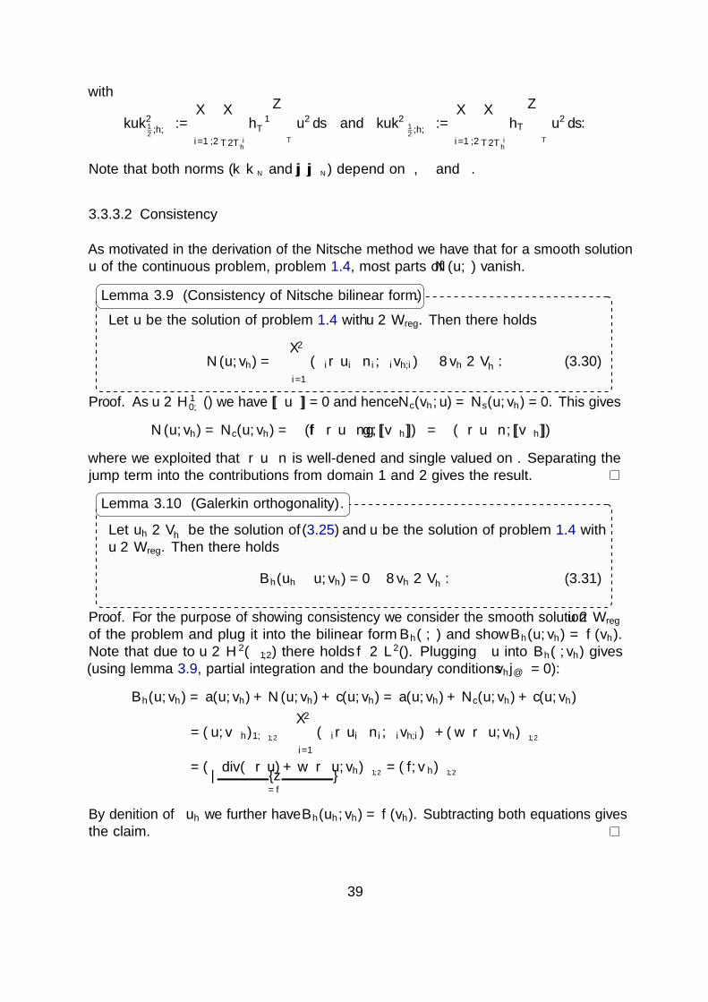
with

‖u‖212,h,Γ

:=∑i=1,2

∑T∈T i

h

h−1T

∫ΓT

u2 ds and ‖u‖2− 1

2,h,Γ

:=∑i=1,2

∑T∈T i

h

hT

∫ΓT

u2 ds.

Note that both norms (‖ · ‖N and ||| · |||N) depend on β, α and λ.

3.3.3.2 Consistency

As motivated in the derivation of the Nitsche method we have that for a smooth solutionu of the continuous problem, problem 1.4, most parts of N(u, ·) vanish.

Let u be the solution of problem 1.4 with u ∈ Wreg. Then there holds

N(u, vh) = −2∑i=1

(αi∇ui · ni, βivh,i)Γ ∀ vh ∈ V Γh . (3.30)

Lemma 3.9 (Consistency of Nitsche bilinear form).

Proof. As u ∈ H10,β(Ω) we have [[βu]] = 0 and hence Nc(vh, u) = Ns(u, vh) = 0. This gives

N(u, vh) = Nc(u, vh) = −(α∇u · n, [[βvh]])Γ = −(α∇u · n, [[βvh]])Γ

where we exploited that α∇u · n is well-defined and single valued on Γ. Separating thejump term into the contributions from domain 1 and 2 gives the result.

Let uh ∈ V Γh be the solution of (3.25) and u be the solution of problem 1.4 with

u ∈ Wreg. Then there holds

Bh(uh − u, vh) = 0 ∀ vh ∈ V Γh . (3.31)

Lemma 3.10 (Galerkin orthogonality).

Proof. For the purpose of showing consistency we consider the smooth solution u ∈ Wreg

of the problem and plug it into the bilinear form Bh(·, ·) and show Bh(u, vh) = f(vh).Note that due to u ∈ H2(Ω1,2) there holds f ∈ L2(Ω). Plugging u into Bh(·, vh) gives(using lemma 3.9, partial integration and the boundary conditions vh|∂Ω = 0):

Bh(u, vh) = a(u, vh) +N(u, vh) + c(u, vh) = a(u, vh) +Nc(u, vh) + c(u, vh)

= (αu, vh)1,Ω1,2 −2∑i=1

(αi∇ui · ni, βivh,i)Γ + (w · ∇u, vh)Ω1,2

= (−div(α∇u) + w · ∇u︸ ︷︷ ︸=f

, vh)Ω1,2 = (f, vh)Ω1,2

By definition of uh we further have Bh(uh, vh) = f(vh). Subtracting both equations givesthe claim.

39

For an error estimate in the L2β(Ω)-norm we later in section 3.3.3.6 apply the Aubin-

Nitsche trick. For this purpose we pose the homogeneous adjoint problem which coincideswith the original problem as the Laplace-operator is self-adjoint. For clarity we denotethe solution of the “adjoint” problem by w. There holds the following stability statement

Let Ω ⊂ R2 be a convex polygon and Γ be a C2-smooth interface. For f ∈ L2β(Ω)

the solution w ∈ H2β(Ω) of problem 1.4 fulfills

‖w‖2,Ω1,2 ≤ cstab‖f‖0. (3.33)

Lemma 3.11 (H2-Regularity of (adjoint) poisson problem).

Proof. See [CZ98].

As ah(·, ·) is symmetric it is also adjoint consistent in the following sense:

Let w be the solution of the adjoint problem with data f ∈ L2β(Ω). Then there

holdsah(v, w) = (f, v)0 ∀ v ∈ Vreg + V Γ

h (3.34)

Lemma 3.12 (Adjoint consistency).

3.3.3.3 Stability

The crucial component in order to show stability of the Nitsche-XFEM formulation isthe control on the (weighted) normal derivative. In section 3.3.2 we briefly addressedthis point to motivate the hansbo-weighted averaging proposed in [HH02].

If piecewise linear functions (k = 1) are used and the weights κi in the averaging· satisfy the estimate

κ2i ≤ cκ

|Ti||T | (3.35)

for a fixed constant cκ, then there exists a constant ctr independent of α, β, h orthe cut position such that

α−12‖α∇uh · n‖− 1

2,h,Γ ≤

√ctr |√αuh|1,Ω1,2 for all uh ∈ V Γ

h . (3.36)

Lemma 3.13.

Proof. The proof is based on lemma 4 in [HH02]. There exists a fixed number cΓ

independent on h or the cut position so that |ΓT |h ≤ cΓ|T |. As ∇uh = const we can

40

thus deduce

α−1‖α∇uh · n‖2− 1

2,h,Γ≤ 2α−1

∑T∈T Γ

h

∑i=1,2

∫ΓT

hα2iκ

2i ‖∇uh‖2

2 ds

≤ 4∑T∈T Γ

h

∑i=1,2

cΓ|T |αiκ2i

1

|ΓT |

∫ΓT

‖∇uh‖22 ds

≤ 4∑T∈T Γ

h

∑i=1,2

cΓαiκ2i

|T ||Ti|

∫Ti

‖∇uh‖22 dx

≤ 4cΓcκ∑i=1,2

αi|∇uh|21,Ωi.

The claim follows with ctr = 4cΓcκ.

The hansbo-weighting fulfills (3.35) with cκ = 1.Remark 3.3 (Higher order discretizations). To generalize the statement in lemma 3.13w.r.t. the polynomial degree k one has to either adjust the weighting κi or add additionalstabilization terms. In [Mas12] a choice for κi in two dimensions is derived which allowsfor such a generalization. However, the proof of the result as well as the construction ofκi is very technical. A simpler choice is κi = 1 if |Ti| > 1

2|T | and 0 otherwise. We expect

that in that case there holds for all polynomials p and |Ti| > 12|T |

1

|ΓT |

∫ΓT

p(s)2 ds ≤ maxs∈ΓT

p(s)2 ≤ maxx∈Ti

p(x)2 ≤ cp1

|Ti|

∫Ti

p(x)2 dx

with a constant cp only depending on the polynomial degree k. This estimate suffices togeneralize the result in lemma 3.13. For the two-dimensional case this claim also followsdirectly from the analysis in [Mas12] (cf. lemma 3.5 and the prior discussion in thatpaper). Another possibility is a higher order version of the ghost penalty stabilization (seesection 3.4.2) which allows to control the normal derivative at the interface independenton the cut position. We did not investigate this further.

In what follows we assume that κi is chosen such that (3.36) also holds for higher orderdiscretizations. This implies the following

On V Γh the norms ‖ · ‖N and ||| · |||N are equivalent, that means for every uh ∈ V Γ

h

there holds‖uh‖N ≤ |||uh|||N ≤ ce‖uh‖N. (3.38)

with ce =√

1 + ctr.

Lemma 3.14.

Proof. The left inequality is trivial. For the right inequality consider that the part ofthe norm ||| · |||N that involves normal derivatives can be bounded with the ‖ · ‖1,Ω1,2 seminorm using lemma 3.13.

41

We derive an ellipticity result for ah(·, ·):

For λ > cλ := max4ctr, 1 there holds

ah(uh, uh) ≥ ga‖uh‖2N for all uh ∈ V Γ

h .

with ga = αmin

2α.

Lemma 3.15.

Proof. There holds

Nc(uh, uh) = −∫

Γ

α∇ · n[[βu]] ds ≤ α−12‖α∇u · n‖− 1

2,h,Γ α

12‖[[βu]]‖ 1

2,h,Γ

≤ ctr

2γ|√αu|21,Ω1,2

+ αγ

2‖[[βu]]‖2

12,h,Γ

for any γ > 0 where we used lemma 3.13. Now setting γ = 2ctr we get

2Nc(uh, uh) ≤1

2a(uh, uh) + 2ctrα‖[[βuh]]‖2

12,h,Γ

(3.40)

Let cλ := max4ctr, 1. Then for λ ≥ cλ we have

2Nc(uh, uh) ≤1

2a(uh, uh) +

1

2Ns(uh, uh).

It easily follows

ah(uh, uh) ≥ a(uh, uh)− 2Nc(uh, uh) +Ns(uh, uh)

≥ 1

2(a(uh, uh) +Ns(uh, uh)) ≥

αmin

2α‖uh‖2

N.

This implies that the discrete problem has a unique solution.

3.3.3.4 Boundedness

For λ > cλ = max4ctr, 1, there holds

ah(u, vh) ≤ Ga|||u|||N‖vh‖N for all u ∈ Vreg + V Γh , vh ∈ V Γ

h

for a constant Ga =√

3.

Lemma 3.16.

42

Proof. Applying Cauchy-Schwarz for all bilinear forms one after another we get

a(u, v) ≤ αmax|u|1,Ω1,2|vh|1,Ω1,2

Nc(u, vh) ≤ α−12‖α∇u · n‖− 1

2,h,Γ α

12‖[[βvh]]‖ 1

2,h,Γ

Nc(vh, u) ≤ α−12‖α∇vh · n‖− 1

2,h,Γ α

12‖[[βu]]‖ 1

2,h,Γ

≤ √ctr|√αvh|1,Ω1,2 α

12‖[[βu]]‖ 1

2,h,Γ

Ns(u, vh) ≤ λ12 α

12‖[[βu]]‖ 1

2,h,Γ λ

12 α

12‖[[βvh]]‖ 1

2,h,Γ

With λ > max4ctr, 1 we get

ah(u, vh) ≤√

3|||u|||N‖vh‖N

which implies the claim.

3.3.3.5 Interpolation error

In the analysis of the Nitsche-XFEM method an interpolation operator IΓh : Vreg → V Γ

h

plays an important role. We recall the extension operator Ei and the restriction operatorRi introduced in section 2.3. Let Ih : H2(Ω) ∩ H1

0 (Ω) → Vh be the standard nodalinterpolation operator corresponding to the space Vh of continuous finite elements ofdegree k. The XFEM interpolation operator is given by

IΓh = R1IhE1R1 +R2IhE2R2. (3.42)

For the interpolation operator IΓh optimal (local) interpolation error bounds can easily

be derived

Let u ∈ Vreg ∩Hm(Ω1,2), m ≥ 2 and IΓh be the interpolation operator into V Γ

h theXFEM finite element space of (continuous) piecewise polynomials of degree k ≥ 1as in (3.42). With eI := u − IΓ

hu, ui = EiRiu, l := mink,m − 1 and i = 1, 2there hold the following local interpolation error bounds for T ∈ Th.

‖eI‖20,Ti≤ch2l+2

T ‖ui‖2l+1,T (3.43a)

|eI |21,Ti≤ch2lT ‖ui‖2

l+1,T (3.43b)

‖RieI‖212,h,ΓT≤ch2l

T ‖ui‖2l+1,T (3.43c)

‖∇RieI ·n‖2− 1

2,h,ΓT≤ch2l

T ‖ui‖2l+1,T (3.43d)

Lemma 3.17.

Proof. The results in (3.43a) and (3.43b) are known in the literature, see for instance [HH02,Reu08] and have been discussed in the introduction of the space V Γ

h . The results in(3.43c), (3.43d), are derived in [HH02]. The essential ingredient is the following result:

‖w‖2L2(ΓT ) ≤ c

(h−1T ‖w‖2

L2(T ) + hT |w|21,T)

for all w ∈ H1(T ),

43

which holds for all T ∈ T Γh and with a constant c that is independent of the shape

regularity of Ti, cf. [HH02, GR11]. We give the proof of (3.43c) and (3.43d):

‖RieI‖212,h,ΓT

= h−1T ‖EiRieI‖2

L2(ΓT ) ≤ c(h−2T ‖EiRieI‖2

L2(T ) + |EiRieI |21,T)

≤ ch2lT ‖ui‖2

l+1,T ⇒ (3.43c),

‖∇RieI ·n‖2− 1

2,h,ΓT≤ hT‖∇EiRieI‖2

L2(ΓT ) ≤ c(‖∇EiRieI‖2

L2(T ) + h2T |∇EiRieI |21,T

)≤ ch2l

T ‖ui‖2l+1,T ⇒ (3.43d).

Let u ∈ Vreg ∩ Hm(Ω1,2) and IΓh as in lemma 3.17. Assume the family of

triangulations is quasi-uniform so that hT ≤ ch. With eI := u − IΓhu and

l := mink,m− 1 there holds

‖eI‖0,Ω1,2≤chl+1‖u‖l+1,Ω1,2 (3.44a)

|eI |1,Ω1,2≤chl‖u‖l+1,Ω1,2 (3.44b)

‖RieI‖ 12,h,Γ≤chl‖u‖l+1,Ωi

(3.44c)

‖∇RieI ·n‖− 12,h,Γ≤chl‖u‖l+1,Ωi

(3.44d)

Lemma 3.18.

Proof. Using quasi-uniformity for the estimates in lemma 3.17 and in addition makinguse of the continuity of the extension operator ‖EiRiu‖l+1,Ω ≤ c‖u‖l+1,Ωi

directly givesthe estimates.

For the norms ‖ · ‖N and ||| · |||N we can directly conclude interpolation bounds using theabove estimates.

For u ∈ Vreg ∩Hm(Ω1,2), m ≥ 2 and l := mink,m− 1 the following interpolationerror bound holds on a quasi-uniform family of triangulations with mesh size h:

‖u− IΓhu‖N ≤ |||u− IΓ

hu|||N ≤ c√αλhl‖u‖l+1,Ω1,2 (3.45)

Lemma 3.19.

3.3.3.6 A priori error estimates

Let uh ∈ V Γh be the solution of (3.25) with λ > cλ and u be the solution of

problem 1.4 with u ∈ Wreg. There holds, with ga, Ga as before

‖u− uh‖N ≤ |||u− uh|||N ≤ (1 +Ga

gace) inf

vh∈V Γh

|||u− vh|||N. (3.46a)

Lemma 3.20 (Modified Cea’s lemma).

44

Proof. With the triangle inequality we split the error into two parts. We introduce a newdiscrete function vh which is arbitrary at this point but will be the best approximationto u in V Γ

h later. We define ea := u− vh what is going to represent the approximationerror and ed := vh − uh ∈ V Γ

h what is denoted as the discrete error:

‖u− uh‖2N ≤ ‖ed‖2

N + ‖ea‖2N, |||u− uh|||2N ≤ |||ed|||2N + |||ea|||2N,

For the discrete error we can apply (in order) lemma 3.14, theorem 3.15, lemma 3.9 andtheorem 3.16 to bound the discrete error by the approximation error:

c−1e |||ed|||N‖ed‖N ≤ ‖vh − uh‖2

N ≤1

gaah(vh − uh, vh − uh)

=1

gaah(vh − u, vh − uh)

≤ Ga

ga|||ea|||N‖ed‖N

⇒ ‖ed‖N ≤ |||ed|||N ≤Ga

gace|||ea|||N

Putting all together concludes the proof.

Let uh ∈ V Γh be the solution of (3.25) and u be the solution of problem 1.4 with

u ∈ Wreg ∩Hm(Ω1,2). Define l := mink,m− 1 and assume Th is quasi-uniformwith mesh size h. Then there holds

‖u− uh‖N ≤ |||u− uh|||N ≤ c√αλhl‖u‖l+1,Ω1,2 . (3.48)

Lemma 3.21 (Error bound in ‖ · ‖N-norm).

Proof. Combine lemma 3.20 and the approximation results in lemma 3.19.

With Ph ≤ 1 this implies for sufficiently smooth functions u

|u− uh|1,Ω1,2 ≤ c√λhk‖u‖k+1,Ω1,2 , (3.49a)

‖[[βuh]]‖Γ ≤ c hk+ 12‖u‖k+1,Ω1,2 , (3.49b)

‖α∇u · n‖Γ ≤ c α√λhk−

12‖u‖k+1,Ω1,2 . (3.49c)

Duality arguments.

45

Let uh ∈ V Γh be the solution of (3.25) and u be the solution of problem 1.4 with

u ∈ Vreg ∩Hm(Ω1,2). Assuming a quasi-uniform mesh with mesh size h and Ph ≤ 1there holds (with l := mink,m− 1)

‖u− uh‖0 ≤ c√αλh|||u− uh|||N (3.50)

≤ c α λ hl+1‖u‖2,Ω1,2 (3.51)

Lemma 3.22 (Error bound in ‖ · ‖0).

Proof. We consider the adjoint problem, problem 1.4, with data f = u− uh ∈ L2(Ω) anddenote the corresponding solution as w. We exploit adjoint consistency (lemma 3.12),Galerkin orthogonality of the primal problem (lemma 3.9) and continuity (theorem 3.16)to get (for any wh ∈ V Γ

h )

‖u− uh‖20 = (u− uh, u− uh)0 = ah(u− uh, w) (3.52a)

= ah(u− uh, w − wh) ≤ Ga|||u− uh|||N|||w − wh|||N. (3.52b)

Now choose wh = IΓhw and apply the previously used approximation results to get

‖u− uh‖20 ≤ c

√αλhGa|||u− uh|||N‖w‖2,Ω1,2 .

Applying the stability estimate of the (adjoint) problem (see lemma 3.11) to bound

‖w‖2,Ω1,2 ≤ cstab‖f‖0 = cstab‖u− uh‖0

finally yields‖u− uh‖0 ≤ c cstab

√αλhGa|||u− uh|||N.

Now plugging in the result in lemma 3.21 concludes the proof.

3.4 Boundary problems on unfitted domains

As a last class of problems we consider a one-domain problem with an unfitted interface

− div(∇u) = f in Ω, (3.53a)

u = gD on ∂Ω. (3.53b)

Problem 3.4.

46

3.4.1 The Nitsche formulation

We consider the fictitious domain space V ficth = v ∈ H1(Ω), v|T ∗ ∈ P k(T ∗), T ∗ =

T ∩ Ω, T ∈ Th. A Nitsche formulation of this kind of problem is easily transfered fromthe fitted problem. Find uh ∈ V fict

h , such that∫Ω

∇uh∇vhds−∫∂Ω

∇uh · n vhds−∫∂Ω

∇vh · nuhds +

∫∂Ω

λ

huhvhds

= 〈f, vh〉+

∫∂Ω

gD(−∇vh · n +λ

hv)ds ∀ vh ∈ V fict

h

(3.54)

3.4.1.1 Stability issues

The problem of the formulation in (3.54) is the fact that stability is no longer givenindependent of the interface position. We have

‖∇uh · n‖− 12,h,∂Ω ≤ c‖uh‖1,Ω

for a constant c depending on the shape regularity of T ∗ (and not T ! ). If the shaperegularity of T ∗ is given bounded (control on interface position) and λ is chosen sufficientlylarge, the Nitsche formulation is stable, consistent and results in optimal order errorbehavior. To have the control on the shape regularity of T ∗ for h→ 0 is in general notpossible.

In the case of two domains and an interface flux, we could use the weighting in the flux∇uh · n to obtain the inverse trace inequality indepent of the shape regularity of T ∗

(only depending on the shape regularity of T ).

A stabilization method which cures the stability problem of the fictitious domain methodis the so-called Ghost penalty method which we briefly discuss in the next section.

3.4.2 Ghost penalty

In a series of papers [Bur10, BH10, BH12, BZ12] Burman et al. suggested an additionalstabilization mechanism which enhances the robustness of the Nitsche formulation w.r.t.the interface cut position.

By introducing an additional term, the “ghost penalty” stabilization, introduces astiffness which is independent on the cut position within individual elements. We brieflypresent the stabilization with the “ghost penalty” method for piecewise linear functions(k = 1).

We introduce the set of faces within the band of cut elements

F∂Ω := F = Ta ∩ Tb, Ta 6= Tb, Ta, Tb ∈ Ω+, Ta or Tb ∈ T Γh . (3.55)

47

On this set we add the stabilization bilinear form

J(uh, vh) :=∑

F∈F∂Ω

γJhF ([[∇Ehuh · n]], [[∇Ehvh · n]])F , uh, vh ∈ V Γh (3.56)

with Eh the canonical extension from Ω to Ω+ of discrete functions from V ficth , hF =

maxhTa , hTb where F = Ta ∩ Tb and γJ the stabilization parameter. This additionalterm penalizes discontinuities in the derivative within the band of cut elements. Notethat the penalty is imposed not only within the domain Ω, but also on the extensionof the functions into Ω+

i . Therefore this stabilization term is independent on the cutposition within the elements which results in the robustness of the method. The crucialpoint of the method is the following idea.

Consider an element T ∈ T ∂Ωh and assume that a neighbor TN ∈ Th \ T Γ

h with T ∩ TN =F 6= ∅ exists. We have (with c a generic constant) under the assumption of shaperegularity (|T | ≤ c|TN |, |T | ≤ chF |F |) for u ∈ H2(Th)

‖∇uh · n‖2− 1

2,h,ΓT

≤ |ΓT |hT ‖∇uh|T‖22 (3.57a)

≤ c|T |(‖∇uh|TN‖22 + ‖[[∇uh]]‖2

2) (3.57b)

≤ c(‖∇uh‖2L2(TN ) + hF‖[[∇Ei,huh · n]]‖2

L2(F )). (3.57c)

The result can be generalized to arbitrary elements in T Γh under reasonable (milder)

assumptions, see [BH12] for details. In consequence this estimate states that the normalderivative on the interface can be controlled by the | · |1-semi-norm and the stabilizationterm independent of the cut position.Remark 3.4 (Higher order ghost penalty). The ghost penalty method has a generalizationto higher order by adding penalty-terms also for higher order derivatives across the facetsnear the boundary.Remark 3.5 (Ghost penalty for Nitsche-XFEM). In the context of interface problemthe “ghost penalty” stabilization is interesting in cases where the weights of the averagingoperator should be significantly different from the hansbo-choice, for instance for largecontrast problems (see [BZ12]). In this case the Nitsche-XFEM discretization lacksstability (and suffers from arising ill-conditioned linear systems). By adding the “ghostpenalty” stabilization the averaging operator is freed from the constraint that has beennecessary to ensure stability (essentially (3.27)).Remark 3.6 (Alternative stabilization). Another approach to improve the robustness ofthe Nitsche-XFEM formulation w.r.t. the dependency on the cut position is discussed in[HR09]. In that paper a stabilized Lagrange multiplier approach (cf. section 3.1.2) for afictitious domain problem is considered. In the consistent stabilization term that is added(cf. (3.6)) the normal derivative is replaced with a (weakly) consistent representative ofthe normal derivative. This is chosen such that forming the gradient on elements withsmall cuts is avoided.Remark 3.7 (Conditioning). The Ghost penalty method ensures that conditioning ofthe resulting system matrix is well-behaved. This holds true for boundary and interfaceproblems. Note that even for the interface problem with the hansbo-averaging (where

48

stability is not a problem) the resulting system matrix is ill-conditioned. In contrast to theboundary problem this can however be easily fixed by suitable preconditioning strategieswhich is discussed in the next section.

49

3.5 Preconditioning of linear systems

In this section we discuss the conditioning and preconditiong strategies for the linearsystems arising from Nitsche-XFEM discretizations for unfitted interface problems. Theresults in this section have also been published in [LR14].

Let G(x) be the Galerkin isomorphism

G : RN → V Γh (3.58)

s.t. G(x) = u =∑N

k=1 xkϕk with N = dim(V Γh ). Let A be the system matrix

of the bilinear form ah(·, ·) in (3.24) in the sense that Ai,j = a(ϕj, ϕi) or xTAx =ah(G(x),G(x)).

As a first quantity of interest we consider the spectral condition number κ(A) = λmax/λmin

where λmax and λmin are the largest and the smallest eigenvalues of the (symmetric positivedefinite) system matrix. In [BZ12] it is shown that κ(A) depends on how the interfacecuts an element. In that paper an indicator ν for “small cut” situations is defined:

ν := mini=1,2

minV ∈V,

xV ∈ΩΓ\Ωi

|ωV | ∩ Ωi

|ωV |. (3.59)

Here, V is the set of vertices V of the triangulation Th and xV is the correspondingcoordinate in Ω, ωV = T ∈ T ,xV ∈ T denotes the patch of elements around a vertexV . For ν 0 we have κ(A)∞, s.t. the problem becomes (very) ill-conditioned.

We consider a test case which allows to easily generate situation with nu 0. Weconsider a “rounded square” as depicted in Figure 3.5.1. By shifting the interface

Γ

d dr r

d

d

r

r

x0

Figure 3.5.1: Geometrical setup of considered test case.

through

• an unstructured and

50

• a structured mesh

we are able to investigate the performance of linear solvers and preconditioners and thedependency on the interface position. We consider the two-domain Poisson problem with(α1, α2) = (3, 2) and (β1, β2) = (2, 1) and restrict to the case of piecewise linear functions,k = 1. Before we consider the example, we use a transformation as discussed in the nextsection.

3.5.1 Basis transformation (β → 1)

The discrete problem arising from a Nitsche-XFEM discretization of the two-domainPoisson problem can be transformed in order to get rid of the parameter β (resulting inβ = 1).

Note that for every v ∈ V Γh there holds βv ∈ V Γ

h et vice versa. Let N = dim(V Γh ). If

we replace the basis U = ϕj(x)j=1,..,N with W = β−1(x)ϕj(x)j=1,..,N we neitherchange the test nor the ansatz space und therefore the solution stays the same. Howeverthe representation of the solution in terms of the coefficient vectors is different. Let udenote the coefficient vector corresponding to the basis U and w the coefficient vectorcorresponding to the basis W with (scalar) components uj and wj, respectively. Thenwe have for u ∈ V Γ

h

u(x) =N∑j=1

ujϕj(x) =N∑j=1

wjβ−1(x)ϕj(x). (3.60)

Between U and W we define the (mixed) mass matrices MUU , MUW ∈ Rn×n and thetransformation matrix T ∈ Rn×n:

MUUk,j :=

∫Ω

ϕkϕj dx, MUWk,j :=

∫Ω

β−1ϕkϕj dx, T :=(MUU)−1MUW . (3.61)

Note that the transformation from one basis into another is not a local problem, it involvesthe solution with a global mass matrix. The solution of a mass matrix problem, however,can be obtained efficiently using a diagonally preconditioned CG, cf. [Reu08].

If we use the basis W to formulate our linear systems, the system matrix changes to

Ak,j =(α∇ϕk,∇ϕj)L2(Ω1,2) − (α∇ϕk · n, [[ϕj]])L2(Γ)

− (α∇ϕj · n, [[ϕk]])L2(Γ) + (¯αλ

h[[ϕk]], [[ϕj]])L2(Γ), j, k = 1, .., N

with α = αβ

and λ = λα/ ¯α. Between the formulation in basis U and W there holds therelation

A = TTAT.

51

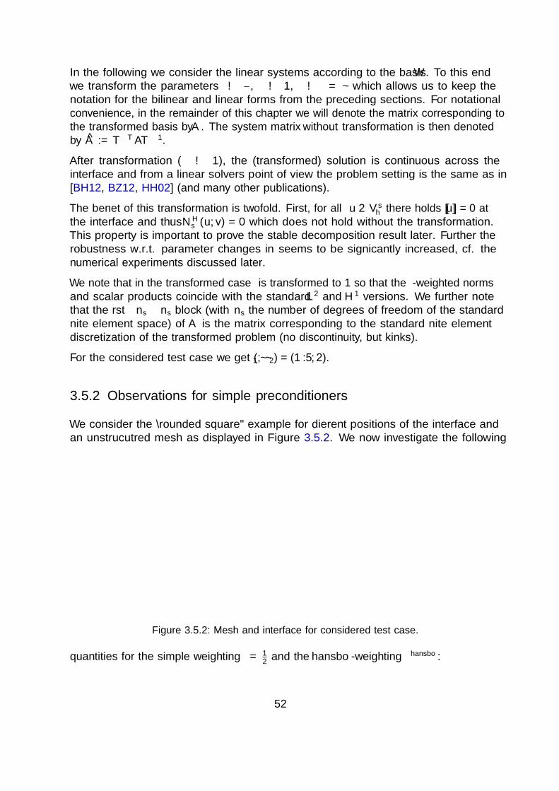
In the following we consider the linear systems according to the basis W . To this endwe transform the parameters α → α

β, β → 1, λ → λα/ ¯α which allows us to keep the

notation for the bilinear and linear forms from the preceding sections. For notationalconvenience, in the remainder of this chapter we will denote the matrix corresponding tothe transformed basis by A. The system matrix without transformation is then denotedby A := T−TAT−1.

After transformation (β → 1), the (transformed) solution is continuous across theinterface and from a linear solvers point of view the problem setting is the same as in[BH12, BZ12, HH02] (and many other publications).

The benefit of this transformation is twofold. First, for all u ∈ V sh there holds [[u]] = 0 at

the interface and thus NHs (u, v) = 0 which does not hold without the transformation.

This property is important to prove the stable decomposition result later. Further therobustness w.r.t. parameter changes in β seems to be significantly increased, cf. thenumerical experiments discussed later.

We note that in the transformed case β is transformed to 1 so that the β-weighted normsand scalar products coincide with the standard L2 and H1 versions. We further notethat the first ns × ns block (with ns the number of degrees of freedom of the standardfinite element space) of A is the matrix corresponding to the standard finite elementdiscretization of the transformed problem (no discontinuity, but kinks).

For the considered test case we get (α1, α2) = (1.5, 2).

3.5.2 Observations for simple preconditioners

We consider the “rounded square” example for different positions of the interface andan unstrucutred mesh as displayed in Figure 3.5.2. We now investigate the following

Γ0.5 Γ0.54

Figure 3.5.2: Mesh and interface for considered test case.

quantities for the simple weighting κ = 12

and the hansbo-weighting κhansbo:

52

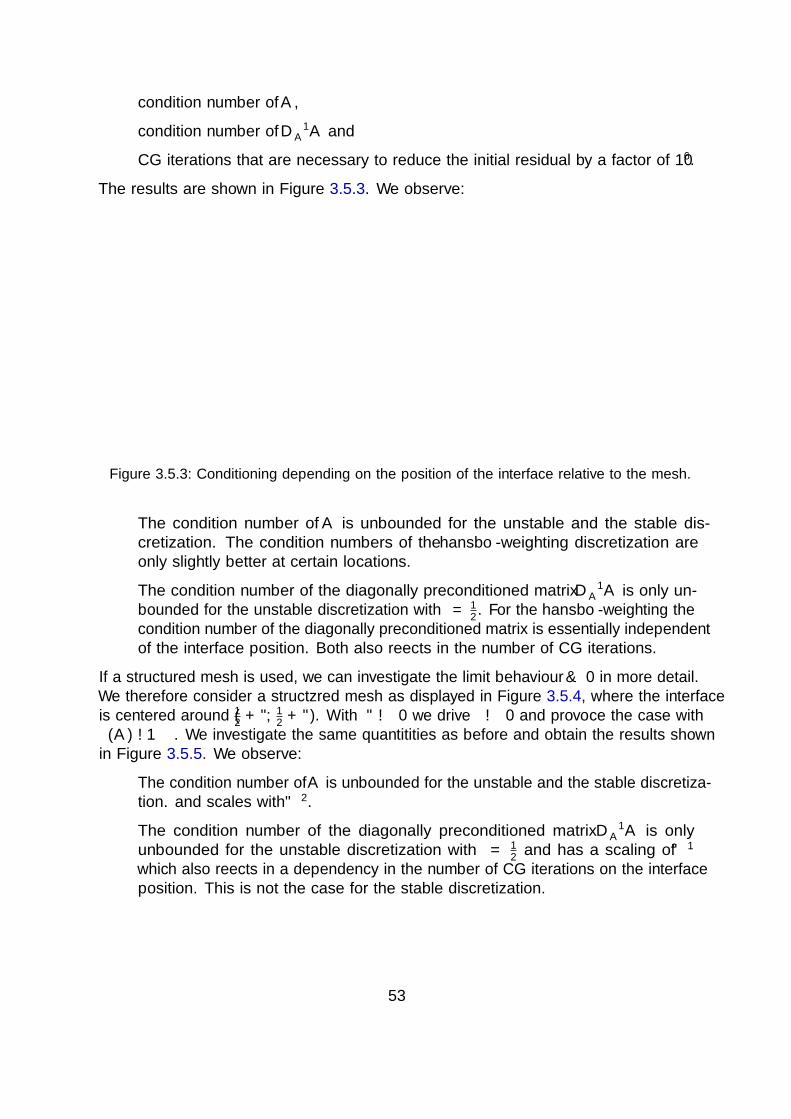
• condition number of A,

• condition number of D−1A A and

• CG iterations that are necessary to reduce the initial residual by a factor of 10−6.

The results are shown in Figure 3.5.3. We observe:

0.46 0.47 0.48 0.49 0.5 0.51 0.52 0.53 0.54

100

102

104

106

108

1010

x0

κ(A) κ(D−1A A)

40

80

CG its.

0.46 0.47 0.48 0.49 0.5 0.51 0.52 0.53 0.54

100

102

104

106

108

1010

x0

κ(A) κ(D−1A A)

40

80

CG its.

Figure 3.5.3: Conditioning depending on the position of the interface relative to the mesh.

• The condition number of A is unbounded for the unstable and the stable dis-cretization. The condition numbers of the hansbo-weighting discretization areonly slightly better at certain locations.

• The condition number of the diagonally preconditioned matrix D−1A A is only un-

bounded for the unstable discretization with κ = 12. For the hansbo-weighting the

condition number of the diagonally preconditioned matrix is essentially independentof the interface position. Both also reflects in the number of CG iterations.

If a structured mesh is used, we can investigate the limit behaviour ν 0 in more detail.We therefore consider a structzred mesh as displayed in Figure 3.5.4, where the interfaceis centered around (1

2+ ε, 1

2+ ε). With ε→ 0 we drive ν → 0 and provoce the case with

κ(A)→∞. We investigate the same quantitities as before and obtain the results shownin Figure 3.5.5. We observe:

• The condition number of A is unbounded for the unstable and the stable discretiza-tion. and scales with ε−2.

• The condition number of the diagonally preconditioned matrix D−1A A is only

unbounded for the unstable discretization with κ = 12

and has a scaling of ε−1

which also reflects in a dependency in the number of CG iterations on the interfaceposition. This is not the case for the stable discretization.

53

κ(D−1A A) (its.) κ1/2 = 0.5

(transf.)

κ = κH(transf.)

κ = κH(untransf.)

Std. FEM(transf.)

L1

max ’∞’( 44) 19.2( 23) 32.7( 30) 14.8( 19)min 61.7( 23) 18.6( 20) 23.4( 25) 14.6( 17)

median 63.7( 26) 18.7( 22) 27.9( 28) 14.7( 19)avg. ’∞’(28.2) 18.8(21.7) 27.8( 28) 14.7( 19)

L2

max ’∞’( 81) 76.5( 41) 107( 53) 62.3( 39)min 78.1( 39) 72.6( 37) 87.8( 45) 61.9( 34)

median 107( 49) 73.0( 40) 94.0( 51) 62.0( 37)avg. ’∞’(49.5) 73.3(40.2) 95.0(50.3) 62.0(37.4)

L3

max ’∞’( 257) 308( 84) 374( 96) 267( 81)min 492( 89) 287( 74) 337( 82) 266( 71)

median 476736( 120) 295( 81) 349( 91) 266( 77)avg. ’∞’( 127) 296(80.3) 349(91.4) 266( 76)

L4

max ( ) 1310( 174) 1390( 186) 1120( 168)min ( ) 1210( 153) 1300( 160) 1120( 147)

median ( ) 1220( 165) 1320( 177) 1120( 158)avg. ( ) 1220( 165) 1320( 178) 1120( 159)

Table 3.5.1: condition and iteration numbers for different refinement levels and different methods(transformed/untransformed, stable/unstable discretization, XFEM/Std. FEM

x0

Figure 3.5.4: Structured mesh and interface for considered test case.

In the next section we discuss why the diagonal preconditioning is already sufficient toremove the dependency on the interface position and more sophisticated preconditioningstrategies.

3.5.3 Preconditioning strategies

We consider preconditioning strategies to solve the linear systems arising from Nitsche-XFEM discretizations.

54

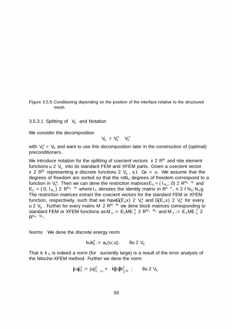
10−8 10−7 10−6 10−5 10−4 10−3 10−2

101

103

105

107

109

1011

1013

ε−2

ε−1

ε−18

ε

κ(A)

κ(D−1A A)

CG its.

10−8 10−7 10−6 10−5 10−4 10−3 10−2

101

103

105

107

109

1011

1013

ε−2

ε

κ(A)

κ(D−1A A)

κ(D−1As

As)

CG its.

Figure 3.5.5: Conditioning depending on the position of the interface relative to the structuredmesh.

3.5.3.1 Splitting of V Γh and Notation

We consider the decompositionV Γh = V s

h ⊕ V xh

with V sh = Vh and want to use this decomposition later in the construction of (optimal)

preconditioners.

We introduce notation for the splitting of coefficient vectors x ∈ RN and finite elementfunctions u ∈ V Γ

h into its standard FEM and XFEM parts. Given a coefficient vectorx ∈ RN representing a discrete function u ∈ V Γ

h , s.t. Gx = u. We assume that thedegrees of freedom are sorted so that the first Ns degrees of freedom correspond to afunction in V s

h . Then we can define the restriction matrices Es = (INs , 0) ∈ RNs×N andEx = (0, INx) ∈ RNx×N where In denotes the identity matrix in Rn×n, n ∈ Ns, Nx.The restriction matrices extract the coefficient vectors for the standard FEM or XFEMfunction, respectively, such that we have G(Esx) ∈ V s

h and G(Exx) ∈ V xh for every

u ∈ V Γh . Further for every matrix M ∈ RN×N we define block matrices corresponding to

standard FEM or XFEM functions as Ms := EsMETs ∈ RNs×Ns and Mx := ExMET

x ∈RNx×Nx .

Norms We define the discrete energy norm

‖u‖2h := ah(u, u), ∀u ∈ V Γ

h

That ‖ · ‖h is indeed a norm (for λ sufficiently large) is a result of the error analysis ofthe Nitsche-XFEM method. Further we define the norm

|||u|||2h := |u|21,Ω1,2+ λ‖[[u]]‖2

12,h,Γ

, ∀u ∈ V Γh

55

Note that both norms are equivalent, i.e. ‖u‖h ' |||u|||h. The equivalence however, is notrobust w.r.t. α. Notet that for u ∈ V s

h , we have |||u|||h = |u|1,Ω1,2 .

3.5.3.2 Stable subspace splittings a.k.a. block preconditioning a.k.a. AdditiveSchwarz method

We want to investigate if the decomposition V Γh = V s

h ⊕ V xh is stable or, in other words,

if the block diagonal matrix corresponding to the standard and the XFEM degrees offreedom is spectrally equivalent to the system matrix.

To show this, we recall

Let A,B ∈ RN×N be s.p.d., then

clxTBx ≤ xTAx ≤ cux

TBx

implies

κ(B−1A) ≤ cucl

=: cκ.

Lemma 3.23.

We consider the block matrix BA =

(As

Ax

)as a preconditioner to A and want to

bound cκ (independent of the interface position). First we show the upper bound, whichis simple:

xTAx = ah(G(x)︸︷︷︸=u

,G(x)) (3.62)

= ah( us︸︷︷︸∈V s

h

+ ux︸︷︷︸∈V x

h

, us + ux) = ah(us, us) + ah(ux, ux) + 2ah(us, ux) (3.63)

≤ 2(ah(us, us) + ah(ux, ux)) (3.64)

= 2(xTETxAExx + xTs ET

s AEsxs) = 2xTBAx (3.65)

Less obvious is the other direction xTAx ≥ clxTBAx. We therefore consider the following

estimate:

xTAx = ‖u‖2h ' |||u|||2h = |||us|||2h + |||ux|||2h + 2(us, ux)1,Ω1,2 + 2λ([[us]]︸︷︷︸

=0

, [[ux]])h, 12,Γ (3.66)

≥ |||us|||2h + |||ux|||2h − cSCS|||us|||2h − cSCS|||ux|||2h (3.67)

= (1− cSCS)(|||us|||2h + |||ux|||2h) (3.68)

' (1− cSCS)(‖us‖2h + ‖ux‖2

h) = (1− cSCS)xTBAx (3.69)

(3.70)

56

We automatically have cSCS ≤ 1. We however need the strengthened Cauchy-Schwarzinequality

(us, ux)1,Ω1,2 ≤ cSCS(|||us|||h|||ux|||h) ∀us ∈ V sh , ux ∈ V x

h

with cSCS < 1. Further we want cSCS to be independent of the position of Γ and h, s.t.the same also holds for cκ.

For every us ∈ V sh and ux ∈ V x

h , there holds

(us, ux)1,Ω1,2 ≤ cSCS|||us|||h|||ux|||h (3.71)

with cSCS independent of h and the position of Γ.

Lemma 3.24 (Strengthened Cauchy-Schwarz inequality).

Idea of proof. The proof is technical and given in [LR14]. We just highlight the mostimportant ideas:

• If there holds(us, ux)1,Ω1,2 ≤ cSCS|us|1,Ω1,2|ux|1,Ω1,2 ,

we are done. Hence, the interesting case is if

1

CSCS|us|1,Ω1,2 |ux|1,Ω1,2 ≤ (us, ux)1,Ω1,2 ≤ |us|1,Ω1,2|ux|1,Ω1,2 ,

which essentially implies that ∇ux ‖ v∇us approximately holds.

• If the gradients of ux are almost parallel, the problem reduces (locally) to a one-dimensional problem where we can contradict the fact that the gradients coincideand [[ux]] = 0 at the interface. Because as soon as the jump has a significantcontribution to the norm the claim automatically holds.

Exercise 3.2. Proof the strengthened Cauchy Schwarz inequality of the previous lemmafor the one dimensional case. (cf. solution A.4)

We thus have that the decomposition V Γh = V s

h ⊕ V xh is a stable space decomposition and

there holdsκ(B−1

A ) ≤ cκ

with cκ independent of the position of Γ and h.

A block diagonal matrix with exact inverses is practically not feasible because the blockmatrices might be to large. Next, we want to replace the block inverses with suitablepreconditioning strategies.

57

3.5.3.3 Preconditiong of blocks

If we have preconditioners Bs and Bx for As and Ax which provide the estimates:

cslxTBsx ≤ xTAsx ≤ csux

TBsx

cxl xTBxx ≤ xTAxx ≤ cxux

TBxx

we can easily deduce that the preconditioner Bc =

(Bs 00 Bx

)provides:

cclxTBcx ≤ xTAxx ≤ ccux

TBcx

with ccl = cl mincsl , cxl and ccu = cu mincsu, cxu. This implies

κ(B−1c A) ≤ ccu

ccl= κ(B−1

A A) · maxcsu, cxumincsl , cxl

It is thus sufficient to find good preconditioners for the blocks.

Preconditioning of block corresponding to Standard FEM degrees of freedom Theupper left block of BA is As with (As)i,j = ah(ϕj, ϕi) = a(ϕj, ϕi) the discretizationmatrix of a standard FEM discretization for −α∆u = f (with discontinuous α). For thiskind of problem optimal preconditioners exist, e.g. Multigrid preconditioners. Hence, weconsider the use such a sophisticated preconditioner.

Preconditoining of the XFEM-block For the XFEM block it turns out that block isspectrally equivalent to its diagonal independent of the interface position Γ and the meshsize h. We thus consider Bx = Dx = diag(Ax).

For the Jacobi preconditioner Dx there holds

cxl xTDxx ≤ xTAxx ≤ cxux

TDx ∀x ∈ RNx

with cxl and cxu independent of the mesh size h and the position of the interface Γ.

Lemma 3.25.

Idea of proof. For a complete proof we again refer to [LR14], but briefly explain the mainidea: Consider an intersected element T ∈ T Γ

h . Further, let one vertex of the simplex Tbe separated from the others by the interface Γ. Then the local bilinear form∫

T1,2

α∇ux∇vx dx

58

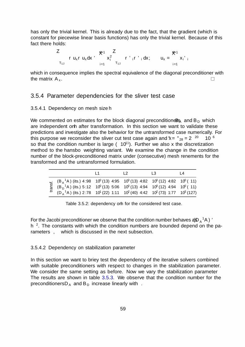
has only the trivial kernel. This is already due to the fact, that the gradient (which isconstant for piecewise linear basis functions) has only the trivial kernel. Because of thisfact there holds:∫

T1,2

α∇ux∇uxdx 'd+1∑i=1

x2i

∫T1,2

α∇ϕi∇ϕi dx, ux =d+1∑i=1

xiϕi

which in consequence implies the spectral equivalence of the diagonal preconditioner withthe matrix Ax.

3.5.4 Parameter dependencies for the sliver test case

3.5.4.1 Dependency on mesh size h

We commented on estimates for the block diagonal preconditioners BA and BD whichare independent on h after transformation. In this section we want to validate thesepredictions and investigate also the behavior for the untransformed case numerically. Forthis purpose we reconsider the sliver cut test case again and fix ε = ε28 = 2−20 ≈ 10−6

so that the condition number is large (≈ 1011). Further we also fix the discretizationmethod to the hansbo weighting variant. We examine the change in the conditionnumber of the block-preconditioned matrix under (consecutive) mesh refinements for thetransformed and the untransformed formulation.

L1 L2 L3 L4

tran

sf. κ(B−1

A A) (its.) 4.98× 100 (13) 4.95× 100 (13) 4.82× 100 (12) 4.82× 100 ( 11)

κ(B−1D A) (its.) 5.12× 100 (13) 5.06× 100 (13) 4.94× 100 (12) 4.94× 100 ( 11)

κ(D−1A A) (its.) 2.78× 101 (22) 1.11× 102 (40) 4.42× 102 (73) 1.77× 103 (127)

Table 3.5.2: dependency on h for the considered test case.

For the Jacobi preconditioner we observe that the condition number behaves as κ(D−1A A) '

h−2. The constants with which the condition numbers are bounded depend on the pa-rameters λ, α which is discussed in the next subsection.

3.5.4.2 Dependency on stabilization parameter λ

In this section we want to briefly test the dependency of the iterative solvers combinedwith suitable preconditioners with respect to changes in the stabilization parameter.We consider the same setting as before. Now we vary the stabilization parameter λ.The results are shown in table 3.5.3. We observe that the condition number for thepreconditioners DA and BD increase linearly with λ.

59

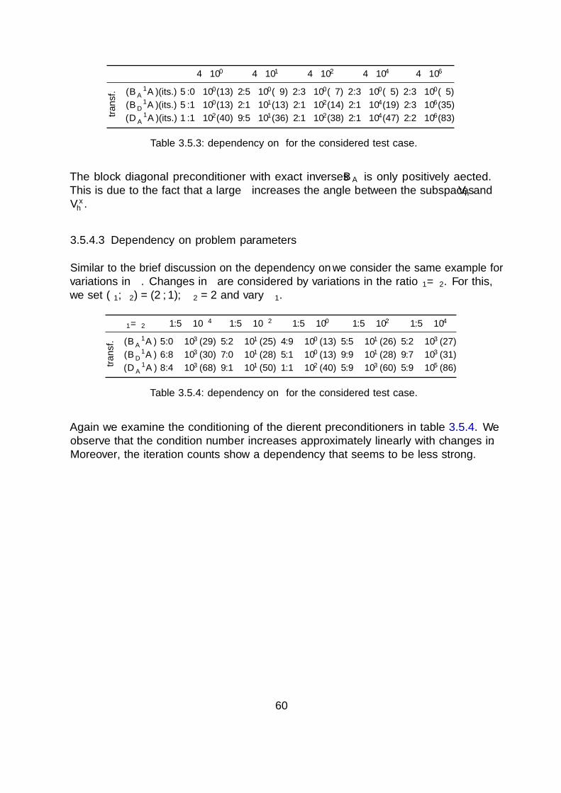
λ 4×100 4×101 4×102 4×104 4×106

tran

sf. κ(B−1

A A)(its.) 5.0×100(13) 2.5×100( 9) 2.3×100( 7) 2.3×100( 5) 2.3×100( 5)

κ(B−1D A)(its.) 5.1×100(13) 2.1×101(13) 2.1×102(14) 2.1×104(19) 2.3×106(35)

κ(D−1A A)(its.) 1.1×102(40) 9.5×101(36) 2.1×102(38) 2.1×104(47) 2.2×106(83)

Table 3.5.3: dependency on λ for the considered test case.

The block diagonal preconditioner with exact inverses BA is only positively affected.This is due to the fact that a large λ increases the angle between the subspaces Vh andV xh .

3.5.4.3 Dependency on problem parameters α

Similar to the brief discussion on the dependency on λ we consider the same example forvariations in α. Changes in α are considered by variations in the ratio α1/α2. For this,we set (β1, β2) = (2, 1), α2 = 2 and vary α1.

α1/α2 1.5× 10−4 1.5× 10−2 1.5× 100 1.5× 102 1.5× 104

tran

sf. κ(B−1

A A) 5.0× 103 (29) 5.2× 101 (25) 4.9× 100 (13) 5.5× 101 (26) 5.2× 103 (27)

κ(B−1D A) 6.8× 103 (30) 7.0× 101 (28) 5.1× 100 (13) 9.9× 101 (28) 9.7× 103 (31)

κ(D−1A A) 8.4× 103 (68) 9.1× 101 (50) 1.1× 102 (40) 5.9× 103 (60) 5.9× 105 (86)

Table 3.5.4: dependency on α for the considered test case.

Again we examine the conditioning of the different preconditioners in table 3.5.4. Weobserve that the condition number increases approximately linearly with changes in α.Moreover, the iteration counts show a dependency that seems to be less strong.

60

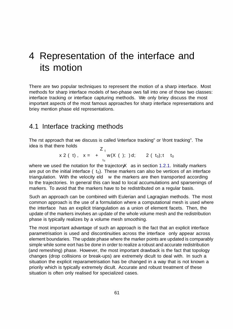
4 Representation of the interface andits motion

There are two popular techniques to represent the motion of a sharp interface. Mostmethods for sharp interface models of two-phase flows fall into one of those two classes:interface tracking or interface capturing methods. We only briefly discuss the mostimportant aspects of the most famous approaches for sharp interface representations andbriefly mention phase field representations.

4.1 Interface tracking methods

The first approach that we discuss is called “interface tracking” or “front tracking”. Theidea is that there holds

x ∈ Γ(t)⇔ x = ξ +

∫ t

t0

w(Xξ(τ), τ) dτ, ξ ∈ Γ(t0), t ≥ t0

where we used the notation for the trajectory Xξ as in section 1.2.1. Initially markersare put on the initial interface Γ(t0). These markers can also be vertices of an interfacetriangulation. With the velocity field w the markers are then transported accordingto the trajectories. In general this can lead to local accumulations and sparsenings ofmarkers. To avoid that the markers have to be redistributed on a regular basis.

Such an approach can be combined with Eulerian and Lagragian methods. The mostcommon approach is the use of a formulation where a computational mesh is used wherethe interface Γ has an explicit triangulation as a union of element facets. Then, theupdate of the markers involves an update of the whole volume mesh and the redistributionphase is typically realizes by a volume mesh smoothing.

The most important advantage of such an approach is the fact that an explicit interfaceparametrisation is used and discontinuities across the interface Γ only appear acrosselement boundaries. The update phase where the marker points are updated is comparablysimple while some effort has be done in order to realize a robust and accurate redistribution(and remeshing) phase. However, the most important drawback is the fact that topologychanges (drop collisions or break-ups) are extremely difficult to deal with. In such asituation the explicit reparametrisation has be changed in a way that is not known apriorily which is typically extremely difficult. Accurate and robust treatment of thesesituation is often only realised for specialized cases.

61

0 0 0

0.3 0.1 0

1 0.9 0.2

Figure 4.2.1: Interface (left), discretization of the volume fraction (middle) and reconstructedinterface (right) for the Volume of Fluid method

4.2 The Volume of Fluid method

Another approach which is an “interface capturing” method is the idea of volumetracking. We want to briefly explain the idea. Let χ1(x, t) be the characteristic functioncorresponding to Ω1(t). Then Γ(t) = ∂Ω1(t) = ∂supp(χ1(·, t)). Then, the immiscibilitycondition VΓ = w · n on Γ translates to

∂tχ1 + w · ∇xχ1 = 0 in D′(ΩT ) := C∞0 (ΩT )′.

where χ1 can also be replaced with a coefficient which is constant inside Ω1, e.g. viscosity.While this formulation is used for the analysis of two-phase flow equations, it is alsothe starting point for a famous numerical method, the Volume of Fluid (VoF) method.Therefore the transport equation

∂tχ1 + w · ∇xχ1 = 0

is formally replaced by

∂t

∫W

χ1dx+

∫∂W

χ1w · nds = 0

for an arbitrary fluid volume W . VoF methods now replaces χ1 with discrete versionsand ensure the conservation of χ1 (typically locally). This is typically done using a FiniteVolume method. Then, by construction the method implements the conservation of fluidvolume which for incompressible flows coincides with the conservation of mass. We brieflysketch how the VoF method operates. In Figure 4.2.1 an example of the most importantingredients is displayed.

The VoF method needs two types of information of the fluids. First, it needs the volumefraction inside each cell. Second, it needs the position of the interface in order to calculatethe fluxes of volume. Starting from an initial interface the construction of the volumefraction values is easy. The other direction however is more involved. Here, the interfaceposition within one cell is reconstructed from the surrounding volume fraction values.For more details we refer to the literature. A comprehensive introduction is given e.g. in[Loc13].

62

Ω1

Ω1 Ω2

Figure 4.3.1: Sketch of two domains and a corresponding level set function fulfilling the signeddistance property.

The VoF method is popular in the engineering community. By construction it has verygood mass-conservation properties and furthermore, topology changes can be handledrelatively easy. The extension of the VoF method away from Finite Volume methods orstructured grids is complicated and only rarely considered.

4.3 The level set method

Another approach to capture the interface uses a different indicator function which hasmore regularity.

The level set equation

We introduce the scalar level set function φ = φ(x, t). This scalar function characterizesthe position of the interface and the domains Ωi in the following way. There holds

φ(x, t)

< 0, x ∈ Ω1(t),> 0, x ∈ Ω2(t),= 0, x ∈ Γ(t).

(4.1)

Thus, given a sufficiently smooth level set function φ, the interface is determined implicitlyby the zero-level of that level set function.

Another desirable property of the level set function is the signed-distance property, whichmeans that the scalar value of φ at a point x does not only indicate the domain in which xlies but further the absolute value of φ defines the (approximate) distance of that point tothe interface Γ(t). φ is called a signed distance function to Γ iff |φ(x, t)| = |dist(x,Γ(t))|and (4.1) holds. If φ only approximately fulfills this property, i.e. |φ(x, t)| ≈ |dist(x,Γ(t))|

63

the level set function φ is called an approximate signed distance function. In figure 4.3.1a level set function which fulfills the signed distance property exactly is shown for asimple two-dimensional configuration.

We assume that the interface motion is completely determined by the velocity field w ofthe flow problem. In that case the interface motion can be described by the followinglinear hyperbolic level set problem.

Given suitable initial values φ0 and boundary conditions φD on the inflow part ofthe boundary ∂Ω−(t) := x ∈ ∂Ω,w(x, t) · n < 0, find φ(x, t) such that

∂tφ+ w · ∇φ = 0 in Ω, φ(x, 0) = φ0 in Ω, φ = φD on ∂Ω−(t). (4.2)

Problem 4.1.

Exercise 4.1. Show that the zero level of the solution of problem 4.1 describes theposition of the interface in the sense that

Γφ(t) := x|φ(x, t) = 0

coincides with

Γs(t) := x |x = x0 +

∫ t

0

w(s(t), t) dt with s(t) = w(s(t), t) and s(0) = x0

with x0 ∈ Γ0 := y|φo(y) = 0. (cf. solution A.5)

Let φ be the exact solution of problem 4.1. Problem 4.1 advects the initial valuesφ(·, 0) = φ0 with the velocity w. Especially the zero-level (the interface Γ) thus followsthe flow w. For the solution of linear hyperbolic transport equation efficient and accuratemethod exist. This make the use of level set methods attractive especially in the finiteelement community. There are however important issues that one should be awareof.

First one should note, that the signed distance property of an initial level set functionφ0 is typically not preserved by the solution of problem 4.1. This typically rendersthe evaluation of the interface position or gradients of φ sensitive to perturbation aftersome time. Furthermore, in the level set equation volume (or mass) is not treatedas a conserved quantity. This implies that as soon as discretization errors occur theconservation of mass can no longer be provided.

For both issues there exist solutions. After several time steps one typically appliessome form of “Re-Initialization” of the level-set. Here, essentially all information exceptfor the interface position is thrown away and a new discrete signed distance functionis constructed. The efficient and accurate realization of such a process is howeverchallenging.

64

4.4 Phase field representation

The idea in a phase field representation is the use of another indicator function which hasa physical meaning and is smooth. Let ρi(x),x ∈ Ω, i = 1, 2 denote the partial densities.As a simplification we assume that we have matched densities, i.e. ρ = ρ1 + ρ2 = const.Then we define the indicator function

c :=ρ1 − ρ2

ρ1 + ρ2

∈ [−1, 1].

In this description the fluids are no longer distinct sharply. There is a transition zone witha thickness > 0. Based on physical principles a phase-field model for the Navier-Stokesequations can be derived:

ρ∂tu + (u · ∇)u = −∇p+ div(µ(c)ε(u))− ε div(∇c∇cT ), (4.3a)

div(u) = 0, (4.3b)

∂tc+ u · ∇c = m∆µchem, µchem = ε−1ψ′0(c)− ε∆c (4.3c)

with a double well potential ψ0, e.g., ψ0(c) = (1− c2)2, and 0 < ε very small.

Problem 4.2.

In this model ε determines the thickness of the transition layer between the two phases.ε is however in most cases chosen as small as possible, i.e. based on numerical ratherthan physical properties. Instead of a transport equation for the indicator c we now havea more complicated convection-diffusion type equation. Here the double well potentialessentially ensures that away from the transition layer the values of c are −1 or 1 while thediffusion operator ensure the smoothness of c across the transition layer. The coefficientµ in the viscous term is now also a smooth function depending on c. Further the surfacetension force is induced by gradients of the order parameter.

Alltogether this model provides smooth quantities for all unknowns which allows for theof standard discretization tools such as finite differences, finite elements or finite volumemethods.

The price that one has to pay is that extremely large gradients (depending on ε) have tobe resolve numerically. Furthermore the fourth order operator acting on c has be dealtwith in an overall very strong nonlinear coupled problem.

Before, we made the assumption of matched densities. In case this assumption does nothold the models are even more complicated.

65

5 Space-Time finite element methodsfor problems with moving interfaces

We now turn back to the original transport problem involving a moving interfaceΓ(t).

5.1 Problem description

We recall the problem under consideration. In this section we consider the followingproblem with a moving interface.

∂tu+ w · ∇u− div(α∇u) = f in Ωi(t), i = 1, 2, t ∈ (0, T ], (5.1a)

[[α∇u · n]]Γ = 0 on Γ(t), t ∈ (0, T ], (5.1b)

[[βu]]Γ = 0 on Γ(t), t ∈ (0, T ], (5.1c)

u(·, 0) =u0 in Ωi(t), i = 1, 2, (5.1d)

u(·, t) = gD on ∂Ω, t ∈ (0, T ]. (5.1e)

Problem 5.1.

Note that due to immiscibility we require w · n = V · n on Γ(t) and div w = 0 in Ωi(t),i = 1, 2, ∀ t ∈ (0, T ]. Here, V · n is the velocity of the interface motion in normaldirection.

5.1.1 Solution strategies

The discretization of problem 5.1 is very challenging due to the fact that the equationsin (5.1a) are defined on time-dependent domains and are coupled through an interfacecondition which leads to discontinuities across the interface. Problems similar to prob-lem 5.1 appear also in other fields, for instance in fluid-structure interaction problems orcombustion. Different approaches exist to tackle the problem. We give a brief overviewof methods which are suitable to deal with problems of the form of problem 5.1.

The balance laws in fluid dynamics are usually described in a fixed control volume, thatis, in an Eulerian frame of reference. Another possibility to state balance equations

66

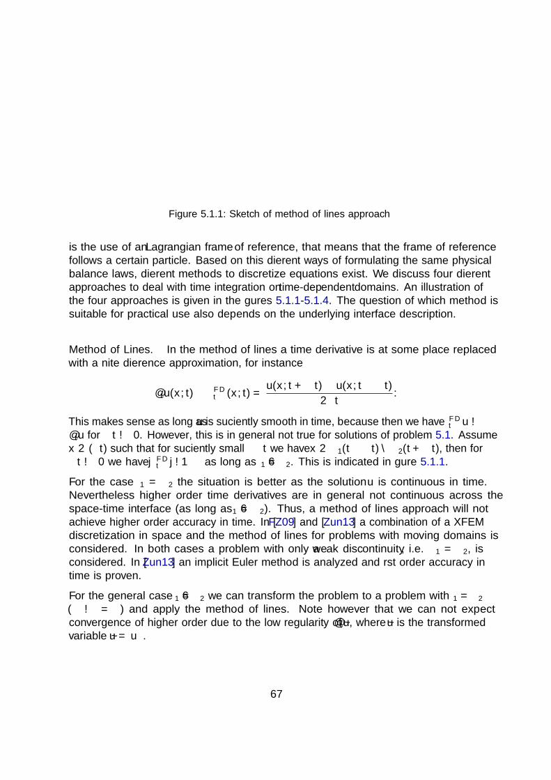
x

t

∂u

∂t6≈ un − un−1

∆t

Γ∗Γ∗

∂u

∂t≈ un − un−1

∆t

Figure 5.1.1: Sketch of method of lines approach

is the use of an Lagrangian frame of reference, that means that the frame of referencefollows a certain particle. Based on this different ways of formulating the same physicalbalance laws, different methods to discretize equations exist. We discuss four differentapproaches to deal with time integration on time-dependent domains. An illustration ofthe four approaches is given in the figures 5.1.1-5.1.4. The question of which method issuitable for practical use also depends on the underlying interface description.

Method of Lines. In the method of lines a time derivative is at some place replacedwith a finite difference approximation, for instance

∂tu(x, t) ≈ δFDt (x, t) =u(x, t+ ∆t)− u(x, t−∆t)

2∆t.

This makes sense as long as u is sufficiently smooth in time, because then we have δFDt u→∂tu for ∆t→ 0. However, this is in general not true for solutions of problem 5.1. Assumex ∈ Γ(t) such that for sufficiently small ∆t we have x ∈ Ω1(t−∆t)∩Ω2(t+ ∆t), then for∆t→ 0 we have |δFDt | → ∞ as long as β1 6= β2. This is indicated in figure 5.1.1.

For the case β1 = β2 the situation is better as the solution u is continuous in time.Nevertheless higher order time derivatives are in general not continuous across thespace-time interface (as long as α1 6= α2). Thus, a method of lines approach will notachieve higher order accuracy in time. In [FZ09] and [Zun13] a combination of a XFEMdiscretization in space and the method of lines for problems with moving domains isconsidered. In both cases a problem with only a weak discontinuity, i.e. β1 = β2, isconsidered. In [Zun13] an implicit Euler method is analyzed and first order accuracy intime is proven.

For the general case β1 6= β2 we can transform the problem to a problem with β1 = β2

(α → α/β) and apply the method of lines. Note however that we can not expectconvergence of higher order due to the low regularity of ∂tu, where u is the transformedvariable u = βu.

67

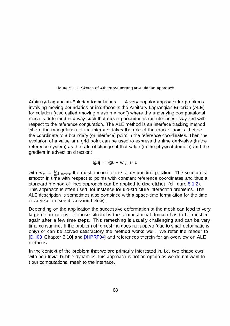
x

t

Γ∗Γ∗

∂u

∂t|ξ ≈

un(ξ)− un−1(ξ)

∆t

Figure 5.1.2: Sketch of Arbitrary-Lagrangian-Eulerian approach.

Arbitrary-Lagrangian-Eulerian formulations. A very popular approach for problemsinvolving moving boundaries or interfaces is the Arbitrary-Lagrangian-Eulerian (ALE)formulation (also called “moving mesh method”) where the underlying computationalmesh is deformed in a way such that moving boundaries (or interfaces) stay fixed withrespect to the reference configuration. The ALE method is an interface tracking methodwhere the triangulation of the interface takes the role of the marker points. Let ξ bethe coordinate of a boundary (or interface) point in the reference coordinates. Then theevolution of a value at a grid point can be used to express the time derivative (in thereference system) as the rate of change of that value (in the physical domain) and thegradient in advection direction:

∂tu|ξ = ∂tu+ wrel · ∇u

with wrel = ∂x∂t|ξ=const the mesh motion at the corresponding position. The solution is

smooth in time with respect to points with constant reference coordinates and thus astandard method of lines approach can be applied to discretize ∂tu|ξ (cf. figure 5.1.2).This approach is often used, for instance for fluid-structure interaction problems. TheALE description is sometimes also combined with a space-time formulation for the timediscretization (see discussion below).

Depending on the application the successive deformation of the mesh can lead to verylarge deformations. In those situations the computational domain has to be meshedagain after a few time steps. This remeshing is usually challenging and can be verytime-consuming. If the problem of remeshing does not appear (due to small deformationsonly) or can be solved satisfactory the method works well. We refer the reader to[DH03, Chapter 3.10] and [DHPRF04] and references therein for an overview on ALEmethods.

In the context of the problem that we are primarily interested in, i.e. two phase flowswith non-trivial bubble dynamics, this approach is not an option as we do not want tofit our computational mesh to the interface.

68

x

t

Γ∗Γ∗

u ≈ un(x) − un−1(Px)

∆t

Figure 5.1.3: Sketch of semi-Lagrangian method.

Semi-Lagrangian methods. Another approach is the use of the so called semi-Lagrangianmethod or characteristic finite element method, where the material derivative u =∂tu + w · ∇u is approximated with a finite difference approximation along a (approx-imated) space-time trajectory. That means one approximates (for an implicit Eulerdiscretization)

u(x, tn) = ∂tu(x, tn) + w · ∇u(x, tn) ≈ u(x, tn)− u(P (x), tn−1)

∆t

where P (x) is the origin of the trajectory through x in the sense that P (x) = y(0) with ythe solution of y = w(y(t), tn−1 + t), y(∆t) = x (cf. figure 5.1.3). This guarantees thatfor every point x in domain i the corresponding origin point P (x) also lies in domain i.Thus the approximation of the time derivative takes place along a line where the solutionis smooth, s.t. simple approximation ideas as in the method of lines can be applied.Another advantage of the method is the fact that due to the Lagrangian handling ofthe time derivative no convection term appears in the resulting equations for the newunknown. One then arrives at a problem of the form

1

∆tun(x)− div(α∇un(x)) = fn(x) +

1

∆tun−1(P (x)) in Ωi, i = 1, 2,

[[α∇un · n]]Γ = 0 on Γ,

[[βun]]Γ = 0 on Γ,

un = gD on ∂Ω.

Problem 5.2.

The Nitsche-XFEM method discussed chapter 3 is very well suited for the discretization ofthis semi-discrete problem. However the approach comes with several disadvantages. In afinite element setting the operator P (x) is non-local which makes it difficult to efficientlyimplement the terms corresponding to the old time values especially on unstructuredmeshes. Also, a suitable choice for P (x) is not obvious if x is close to a Neumann-boundary condition. Furthermore a rigorous error analysis of this kind of methods seems

69

x

t

Γ∗Γ∗

∂u∂t

Figure 5.1.4: Sketch of Space-Time method.

to be very hard. Methods based on the idea of characteristics (or a semi-Lagrangianpoint of view) have been applied for convection-diffusion equations in [DR82, RT02], forthe Navier-Stokes equations in [CHCOB09, ME98], for surfactants equations in [HLZ13]and in [HWGW14] a method combining the semi-Lagrangian point of view with a XFEMdiscretization in space has been considered, however, without any analysis.

Space-Time formulations. The last approach that we want to mention is also the onethat we consider in the remainder of this chapter. The basic idea is to consider theproblem 5.1 directly as a stationary problem in d+1 dimension and to discretize it as such.In order to keep the computational costs comparable to standard time discretizationstrategies (for example the method of lines), the space-time domain is divided into timeslabs which correspond to the time intervals usually used in time stepping methods.Then, a variational formulation is applied which decouples the time slabs such that thecomputational structure is that of a time stepping scheme. We discuss the details in theremaining part of this section.

Discretizations based on space-time formulations have been considered for fluid flowin, for instance [TBML92, TLB92, Beh01, SvdVvD06, SBvdV06, KvdVvdV06, Beh08,Neu13, Wel13]. In [Tho97] the space-time formulation for parabolic problems is dis-cussed and extensively analyzed. In all these publications problems with matchingboundaries(interfaces) in space-time and smooth solutions are considered.

Space-time notation

We adopt and adapt the notation for triangulations, domains, etc. from chapter 2 andintroduce additional notation for space-time related geometries and quantities. Let d bethe spatial dimension of Ω, such that Ω ∈ Rd. Within each time slab Qn := Ω× In, In =(tn−1, tn] we assume that the triangulation of the spatial domain Ω is a shape regulardecomposition into simplices Tn = T. The corresponding characteristic mesh size is

70

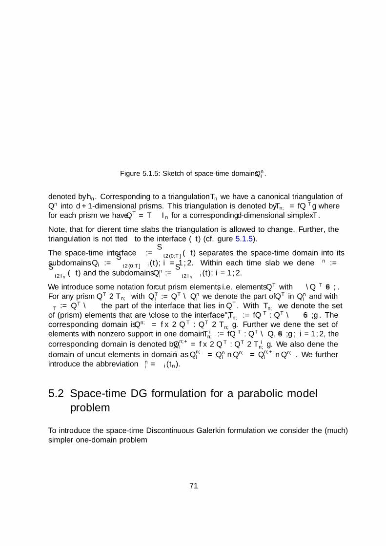
x

t

tn

tn−1

Γ∗Γ∗

Qn2

Qn−11

x

ttn

tn−1

Γ∗Γ∗Qn2 Qn

1

Figure 5.1.5: Sketch of space-time domains Qni .

denoted by hn. Corresponding to a triangulation Tn we have a canonical triangulation ofQn into d+ 1-dimensional prisms. This triangulation is denoted by Tn,∗ = QT wherefor each prism we have QT = T × In for a corresponding d-dimensional simplex T .

Note, that for different time slabs the triangulation is allowed to change. Further, thetriangulation is not fitted to the interface Γ(t) (cf. figure 5.1.5).

The space-time interface Γ∗ :=⋃t∈(0,T ] Γ(t) separates the space-time domain into its

subdomains Qi :=⋃t∈(0,T ] Ωi(t), i = 1, 2. Within each time slab we define Γn∗ :=⋃

t∈In Γ(t) and the subdomains Qni :=

⋃t∈In Ωi(t), i = 1, 2.

We introduce some notation for cut prism elements, i.e. elements QT with Γ∗ ∩QT 6= ∅.For any prism QT ∈ Tn,∗ with QTi := QT ∩Qn

i we denote the part of QT in Qni and with

Γ∗T := QT ∩ Γ∗ the part of the interface that lies in QT . With T Γn,∗ we denote the set

of (prism) elements that are “close to the interface”, T Γn,∗ := QT : QT ∩ Γ∗ 6= ∅. The

corresponding domain is Qn,Γ = x ∈ QT : QT ∈ T Γn,∗. Further we define the set of

elements with nonzero support in one domain: T in,∗ := QT : QT ∩Qi 6= ∅, i = 1, 2, the

corresponding domain is denoted by Qn,+i = x ∈ QT : QT ∈ T in,∗. We also define the

domain of uncut elements in domain i as Qn,−i = Qn

i \Qn,Γ = Qn,+i \Qn,Γ. We further

introduce the abbreviation Ωni = Ωi(tn).

5.2 Space-time DG formulation for a parabolic modelproblem

To introduce the space-time Discontinuous Galerkin formulation we consider the (much)simpler one-domain problem

71

∂tu− div(α∇u) = f in Ω× (0, T ] (5.3a)

u = 0 on ∂Ω× (0, T ], (5.3b)

u =u0 on Ω× 0. (5.3c)

Problem 5.3.

For ease of presentation we assume the use of an equidistant time discretization. Apartitioning of the time interval is given by 0 = t0 < t1 < ... < tN = T with a uniformtime step ∆t = T/N . We define the time interval In = (tn−1, tn] and assume a shaperegular simplicial triangulation T nh of the spatial domain Ω. In general, the triangulationis allowed to change with each time step n. Let Vh be a standard finite element spacecorresponding to T nh . On the time slab Qn := Ω× In we introduce the tensor-productfinite element space

Wn := v : Qn → R|v(x, t) =k∑

m=0

tmϕm(x), ϕm ∈ Vh,m = 0, .., k. (5.4)

Note that due to the tensor-product structure the order of the ansatz functions canbe chosen differently in space and time directions. We typically consider the case ofpiecewise linear functions for Vh combined with linear functions in time (k = 1 in (5.4)).The corresponding finite element space for the whole space-time domain is

W := v : Q→ R|v|Qn ∈ Wn. (5.5)

Note that there is no temporal continuity between the time slabs imposed on W.

The discretization is derived as follows. First we test (5.3a) with a test function v ∈ Wn

and integrate over one time slab Qn. As usual we do partial integration in space for thesecond order term which yields (for a sufficiently smooth function u)∫

Qn

∂tu v + α∇u∇v dx dt =

∫Qn

f v dx dt (5.6)

To abbreviate notation later on, we introduce the (bi)linear forms

ans (u, v) :=

∫Qn

α∇u∇v dx dt, dns (u, v) :=

∫Qn

∂tu v dx dt, fns (v) :=

∫Qn

f v dx dt. (5.7)

We use the subscript s to indicate the correspondence to the simpler problem 5.3. Toinclude information from the past we apply a standard upwind technique. The timederivative can be seen as an advection term in the space-time domain. In that senseΩ× tn−1 is the inflow boundary of Qn where inflow information has to be provided.This is done by adding the upwind stabilization

bns (u, v) :=

∫Ω

[[u]]n−1 vn−1+ dx (5.8)

72

with the time jump and time trace operators

[[u]]n := un+ − un−, un− := u(·, tn), un+ := limε↓0

u(·, tn + ε).

Adding the equations for each time slab n together we get the overall space-time DGdiscretization of problem 5.3. u0

− in the upwind term is given initial data and movedto the r.h.s. side of the variational formulation. For notational convenience we define[[u]]0 = u0

+, s.t. b1(u, v) = (u0+, v

0+). The discrete variational formulation reads as:

Find uh ∈ W such that

Bs(uh, vh) := ds(uh, vh) + as(uh, vh) + bs(uh, vh) = fs(vh) + c0s(vh) ∀ vh ∈ W. (5.9)

with c0s(vh) :=

∫Ωu0 v0

h,+ dx while the other (bi)linear forms are obtained by summing

the corresponding (bi)linear forms over all time slabs, for instance ds(·, ·) =∑N

n=1 dns (·, ·).

Note that the coupling in time has a direction in the sense that the time steps < k donot depend on the solution at time step k. The discretization thus naturally divides intotime stepping problems which can be solved one after another. The problem for eachtime slab n is obtained by testing (5.9) with v ∈ W ∩ v(x, t) = 0, t 6∈ In and reads as:Given un−1

− ∈ L2(Ω) and f ∈ L2(Qn), determine uh ∈ Wn such that for every vh ∈ Wn

there holds

Bn,∗s (uh, vh) := dns (uh, vh) + ans (uh, vh) + bn,∗s (uh, vh) = fns (vh) + cn−1

s (vh)

with bn,∗s (u, v) :=∫

Ωun−1

+ vn−1+ dx and cn−1

s (u, v) :=∫

Ωun−1− vn−1

+ dx. Due to the discontinuous-in-time finite element space W this time discretization is a Discontinuous Galerkin(in time) method. In [Tho97] the method including a thorough error analysis is dis-cussed.Remark 5.1 (Petrov-Galerkin DG methods). In the presented method the test and thesolution space coincide. This is not necessary. A popular alternative is the use of aPetrov-Galerkin method using continuous (in time) finite elements for the solution spacecombined with discontinuous finite elements (in time) of a lower degree for the test space.This reduces the number of unknowns, but still allows for a time stepping procedure. Inthe context of an XFEM finite element space and a two-domain discretization with aspace-time finite element method the use of different spaces for solution and test space isnot straight-forward, cf. remark 5.6. In the following we thus restrict to the discussionof Discontinuous Galerkin in time methods where test and ansatz spaces coincide.Remark 5.2 (Energy-stability). Assume that there is no source term f = 0. A propertyof the exact solution to the problem 5.3, is that the energy of the system can not increase(as long as their are no sources due to f or boundary conditions). Here, the energy isW (u) = 1

2‖u‖2 and there holds ∂tW (u) ≤ 0. A nice property of the DG discretization is

that this property also holds on the discrete level, in the sense 12‖un−‖2

Ω ≤ 12‖un−1− ‖2

Ω, cf.[LR13, lemma 3.5].Remark 5.3 (Stability of the DG time integration method). The discontinuous-in-timeGalerkin method as a time integration method is stable and has the optimal smoothingproperty, but is not A-stable, cf. [GR11, Section 11.5.2].

73

5.3 Space-time extended finite elements

We present the XFEM space analogously to the presentation of the XFEM space forthe stationary problem. Again, we restrict to the case of piecewise bilinear functions(linear in space and linear in time) here. The XFEM space in a space-time setting haspreviously been introduced in [GR11, Chapter 11.5.2], [LR13] and [Leh15a]. The idea of acombination of space-time methods and XFEM has also been suggested in [CB04, CB06]for a one dimensional hyperbolic problem without any error analysis.

The generalization of the XFEM space introduced in chapter 2 is obtained by the use ofa generalization of the restriction operators Ri. The space-time XFEM spaces are givenby

W Γn := Rn

1Wn ⊕Rn2Wn

W Γ := v : Q→ R | v|Qn ∈ W Γn = R1W ⊕R2W.

(5.10)

with the corresponding canonical restrictions Rni on L2(Qn), Ri on L2(Q) given by

Rni v =

v|Qn

ion Qn

i

0 on Qn \Qni ,

Riv =

v|Qi

on Qi

0 on Q \Qi.

We will also use the notation vi := Riv.

We again give a characterization corresponding to the name extended finite elementspace (XFEM) for the case of piecewise linear functions in space and time. Let qjj∈Jbe the nodal basis in the finite element space Vh. The vertex corresponding to qj isdenoted by xj. To each qj there correspond two space-time basis functions, namelyqj,0(x, t) := 1

∆t(tn − t)qj(x) and qj,1(x, t) := 1

∆t(t − tn−1)qj(x).The index set of basis

functions in the space-time finite element space Wn “close to the interface” is givenby

JΓn∗ := (j, 0), (j, 1) | measd(Γn∗ ∩ supp (qj)

)> 0.

Let HΓn∗ be the characteristic function corresponding to Qn2 , i.e. HΓn∗ (x, t) = 1 if

(x, t) ∈ Qn2 and zero otherwise. For each space-time node index (j, `) ∈ JΓn∗ a so-called

enrichment function corresponding to the node (xj, tn−`) is given by

Φj,`(x, t) := |HΓn∗ (x, t)−HΓn∗ (xj, tn−`)|. (5.11)

New basis functions are defined as follows:

qΓn∗

j,` := qj,`Φj,`, (j, `) ∈ JΓn∗ . (5.12)

An illustration for the spatially one-dimensional case is given in figure 5.3.1.

The term HΓn∗ (xj, tn−`) in the definition of Φj,` is constant and may be omitted (as it

doesn’t introduce new functions in the function space), but ensures that qΓn∗

j,` (xj, tn−`) = 0

74

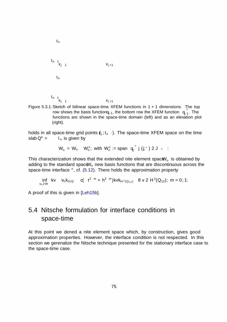
xj−1 xj+1

tn

tn−1

Γ∗

xj−1 xj+1

tn

tn−1

Γ∗

Figure 5.3.1: Sketch of bilinear space-time XFEM functions in 1 + 1 dimensions. The toprow shows the basis function qj,1, the bottom row the XFEM function q

Γn∗

j,1 . Thefunctions are shown in the space-time domain (left) and as an elevation plot(right).

holds in all space-time grid points (xj, tn−`). The space-time XFEM space on the timeslab Qn = Ω× In is given by

W Γn = Wn ⊕W x

n , with W xn := span

q

Γn∗

j,` | (j, `) ∈ JΓn∗

.

This characterization shows that the extended finite element space W Γn is obtained by

adding to the standard space Wn new basis functions that are discontinuous across thespace-time interface Γn∗ , cf. (5.12). There holds the approximation property

infvh∈WΓ

‖v − vh‖m,Q ≤ c(∆t2−m + h2−m)‖v‖H2(Q1,2) ∀ v ∈ H2(Q1,2), m = 0, 1.

A proof of this is given in [Leh15b].

5.4 Nitsche formulation for interface conditions inspace-time

At this point we defined a finite element space which, by construction, gives goodapproximation properties. However, the interface condition is not respected. In thissection we gerenalize the Nitsche technique presented for the stationary interface case tothe space-time case.

75

5.4.1 Derivation of the method

We assume that the solution to problem 5.1 is smooth, multiply (5.1a) with an arbitrarytest function βv ∈ W Γ and integrate over the space-time domain. Afterwards, on everytime slab we apply partial integration in space for the diffusion operator which yields

N∑n=1

(∂tu+ w · ∇u, v)Qn

1,2+ (α∇u,∇v)Qn

1,2

−∫ tn

tn−1

∫Γ(t)

[[α∇u · n βv]]ds dt

= (f, v)Q1,2

(5.13)

To transform the iterated integrals which appear in the Nitsche formulation to an integralon the space-time interface we use the following transformation formula:∫ tn

tn−1

∫Γ(t)

f(s, t) ds dt =

∫Γn∗

f(s)(1 + (w · n)2

)− 12 ds =:

∫Γn∗

f(s)ν(s) ds,

with ν(s) =(1 + (w · n)2

)− 12 and w the (interface) velocity. Note that ds denotes both

the surface measure on Γ(t) as well as on Γ∗. Under the assumption that the space-timeinterface is sufficiently smooth, there holds for a constant c0 > 0

c0 ≤ ν(s) ≤ 1 for all s ∈ Γ∗.

We define the scalar product on the space-time interface (on one time slab)

(u, v)Γn∗ :=

∫Γn∗

u v ds.

We manipulate the normal flux term similar to what we did in chapter 3, where wereplaced [[α∇u ·n βv]] with α∇u ·n[[βv]] due to α∇u ·n being uni-valued at the interface.Similar to what we did for the stationary interface we define

Nnc (u, v) := −(α∇u · n, [[βv]])Γn∗ .

and, with additional symmetry and stabilization terms define

Nn(u, v) :=Nnc (u, v) +Nn

c (v, u) +Nns (u, v), Nn

s (u, v) :=(αλ h−1[[βu]], [[βv]])Γn∗ . (5.14)

We define N(·, ·), Nc(·, ·), Ns(·, ·) by summation over all time slabs, for instance N(·, ·) =∑Nn=1N

n(·, ·). The weights in · are chosen as in the hansbo-choice for the case ofa stationary interface. Take t ∈ In, T ∈ Tn and let Ti(t) := T ∩ Ωi(t). We define theweights

(κi(t))|T :=|Ti(t)||T | . (5.15)

76

Note that those weights only depend on the spatial configuration at a given time t andthere holds κ1(t) + κ2(t) = 1. We define the weighted average

v := κ1(t)(R1v)|Γ(t) + κ2(t)(R2v)|Γ(t). (5.16)

Note that now κi depends on time.

To finish the discretization we need to (weakly) add continuity in time. This is donewith an upwind stabilization term as in (5.8). We define the upwind bilinear form

b(u, v) =N∑n=1

bn(u, v) :=N∑n=1

([[u]]n−1, vn−1+ )Ωn−1

1,2=

N∑n=1

∑i=1,2

∫Ωn−1

i

βi [[u]]n−1 vn−1+ dx. (5.17)

Together, we obtain a discrete variational formulation:Find uh ∈ W Γ such that

B(uh, vh) = f(vh) + c(u0, vh) ∀ vh ∈ W Γ

with B(uh, vh) := d(uh, vh) + a(uh, vh) + b(uh, vh) +N(uh, vh)(5.18)

and the bilinear forms

a(u, v) =N∑n=1

an(u, v) := (α∇u,∇v)Q1,2 , (diffusion) (5.19a)

d(u, v) =N∑n=1

dn(u, v) :=N∑n=1

(∂tu+ w · ∇u, v)Qn1,2, (space-time convection) (5.19b)

c(w, v) := (w, v0+)Ωn−1

1,2. (initial data) (5.19c)

and

f(v) =N∑n=1

fn(v) := (f, v)Qn1,2. (source) (5.19d)

This weak formulation can be rewritten if we apply partial integration on d(·, ·) and makeuse of homogeneous boundary conditions. For all u, v ∈ W Γ +H1(Q1,2) there holds

B(u, v) = B′(u, v) := d′(u, v) + a(u, v) + b′(u, v) +N(u, v) (5.20)

with

d′(u, v) := −N∑n=1

(u, ∂tv + w · ∇v)Qn1,2, (5.21a)

b′(u, v) := −N−1∑n=1

(un−, [[v]]n)Ωn1,2

+ (uN− , vN− )ΩN

1,2. (5.21b)

77

x

ttn

tn−1

Γ∗

Figure 5.4.1: Sketch of a space-time slab where the interface position is changing

The Space-Time-DG Nitsche-XFEM method defined in (5.18) allows for a solution timestep by time step. By testing with a test function which has only support within onetime slab, we get the time slab problem:Find u ∈ W Γ, s.t.

Bn(u, v) = an(u, v) + bn(u, v) + dn(u, v) +Nn(u, v) = fn(v) + cn(un−1, v) (5.22)

where the upwind coupling bi- and linear forms within one time step are

bn(u, v) =∑i=1,2

∫Ωn−1

i

βiun−1+ vn−1

+ dx (5.23)

and

cn(w, v) =∑i=1,2

∫Ωn−1

i

βiwvn−1+ dx. (5.24)

Hence, the computational overhead of the method is determined by the costs for thesetup and the solution of the linear systems arising from (5.22). The efficient solution ofarising linear systems is challenging and topic of ongoing research.Remark 5.4 (Mass conservation). The Space-Time-DG Nitsche-XFEM discretization isglobally mass conserving w.r.t. the discrete time points t = tn. To see that test (5.18)with v = β−1 ∈ W Γ and use the characterization (5.20) to get∫

Ω

u−(·, tN) dx =

∫Ω

u0 dx +

∫Q

f dxdt.

The same mass balance holds for the true solution. For each time slab one gets a (time)local version of this mass balance:∫

Ω

u−(·, tn) dx =

∫Ω

u−(·, tn−1) dx +

∫Qn

f dxdt.

Remark 5.5 (Integration on space-time domains). An implementation of the discretiza-tion method defined in (5.18) or (5.22) needs to compute integrals on (possibly cut) prisms.Especially for the spatially three dimensional case this is challenging and non-standard.A solution strategy is presented in [Leh15a]. In the remainder of this chapter we assumethat space-time integrals can be computed exactly.

78

Remark 5.6 (Petrov-Galerkin DG formulations). In space-time formulations it is, ingeneral, not necessary to choose the same test as ansatz space, cf. remark 5.1. Incombination with XFEM it is however not clear how a well-posed Petrov-Galerkin versionof the presented XFEM discretization can be achieved. We explain the problem. Considera test space with piecewise constants in time W 0 and the ansatz space with piecewiselinears in time W 1. Both are enriched with the XFEM approach resulting in spaces W Γ,1

and W Γ,1. In figure 5.4.1 the cut elements change between the time steps. The resultingXFEM enrichment for W 1 and W 0 results in six additional degrees of freedoms in theinterface region for W Γ,1 and only three for W Γ,0. Hence, the total number of unknownsof test and ansatz space do not match. A possible remedy could be an enrichment of W Γ,0

by discontinuous (in time) piecewise linear XFEM functions in the interface region. Wedid not investigate this further.Remark 5.7 (Weightings in the average). From a computational point of view thesuggested average in (5.16) is computationally inconvenient as in a space-time imple-mentation of the cut elements (prisms) integration is done on space-time geometries.The evaluation of κi(t), however, needs geometry information of a slice through a space-time geometry. Within each cut element κi(t) has to be evaluated at several space-timeintegration points. A more “natural” weighting adjusts the weights to the space-timemeasures:

κi|QT :=|QTi ||QT | . (5.25)

Hence, κi is constant within each space-time element (prism). Note that the measures|QTi | and |QT | have to be computed anyway, that means that this choice is computationallycheap. This choice seems to be suitable in practice. Stability, however, is proven moreeasily for the time-dependent weight.Remark 5.8 (Non-symmetric Nitsche variants). Instead of the symmetric Nitsche for-mulation N(u, v) = Nc(u, v) + Nc(v, u) + Ns(u, v) one can also use nonsymmetric orincomplete formulations as Nns(u, v) = Nc(u, v) − Nc(v, u) + Ns(u, v) or Ninc(u, v) =Nc(u, v)+Ns(u, v). For both modifications the stability analysis discussed later also applies.For the nonsymmetric formulation the analysis is actually simpler as Nns(u, u) = Ns(u, u).Note that the loss of symmetry also implies a lack of adjoint consistency. In the remainderwe thus only consider the symmetric formulation.

79

A Exercise solutions

Solution A.1 (to exercise 1.1). The fluid is at rest, i.e. we have for the momentumequation in the subdomains (ρ = ρ1)

p = p0i + ρ(x− x0

i ,g).

with p0i a reference pressure at location x0

i .

The interface condition [[u]] = 0 is automatically fulfilled. For the other condition on themomentum balance we have

• κ = d−1R

= 2 and

• σi = −piIwhich gives

[[σ · nΓ]] = −[[p]]nΓ!

= −2τnΓ.

Hence p1 − p2 = [[p]] = 2τ . Let us fix p0 = p02 as the Ω2-sided pressure at x0 = x0

2 =

(0, 0,−1) ∈ Γ and set x01 = x0. Then we have (p1 − p2)(x0) = p0

1 − p02

!= 2τ and hence

p2 = p0 + ρ(x− x0,g), p1 = p2 + 2τ = p0 + 2τ + ρ(x− x0,g).

Note, that the pressure is only determined up to a constant as there are no boundaryconditions on it.

The relation [[p]] = τκ = 2τ/R for spherical interfaces is known as the Young-Laplace law.

Solution A.2 (to exercise 2.1). Obviously on all elements except for T Γ, the elementwhich is intersected by Γ, the best approximation of u is exact and we have

infvh∈V n

h

‖vh − u‖L2(Ω) = infvh∈Pk(TΓ)

‖vh − u‖L2(TΓ).

Via transformation to the reference element T = [0, 1] we get the position of thecorresponding transformed interface Γ as 1

3or 2

3. Both cases are equivalent due to

symmetry. We thus have

infvh∈V n

h

‖vh − u‖L2(Ω) = infvh∈Pk(TΓ)

‖vh − u‖L2(TΓ) =√h infvh∈Pk([0,1])

‖vh − u Φ‖L2([0,1]).

80

So we are left with the task of approximating a discontinuous function on the referenceelement with univariant polynomials. As the discontinuous functions are not in Pk([0, 1])is a constant C = infvh∈Pk([0,1]) ‖vh − u Φ‖L2([0,1]) which is independent of the mesh sizeh.

As for the space V k,conth of continuous piecewise functions of degree k, we have V k,cont

h ⊂V k,disch , there holds:

infvh∈V n,disc

h

‖vh − u‖L2(Ω) ≤ infvh∈V n,cont

h

‖vh − u‖L2(Ω) = C√h

Solution A.3 (to exercise 3.1). On the continuous level we have V = (H1(Ω), ‖ · ‖1,h)and Q = (L2(∂Ω), ‖ · ‖− 1

2,h,∂Ω). We check if the requirements of Brezzi’s Theorem are

fulfilled: There holds

• continuity of a:a(u, v) ≤ ‖u‖1,h‖v‖1,h,

• continuity of b:

b(u, v) =

∫∂Ω

uqds ≤ ‖u‖1,h‖q‖− 12,h,∂Ω,

• kernel-ellipticity of a (on the kernel of b):

a(u, v)(≥)= ‖u‖2

1 = ‖u‖21,h ∀u ∈ H1

0 (Ω) = V ∗ = v ∈ H1, tr|∂Ωv = 0

• and the inf-sup-condition. For every q ∈ L2(∂Ω), we construct u∗(q) as the solutionof ∆u∗ = 0 in Ω and u∗ = q on ∂Ω and thereby get

– Matching of boundary values u∗ = q on ∂Ω

– Bound of the ‖ · ‖1-norm by the data: ‖u∗‖1 ≤ C‖ u∗︸︷︷︸=q

‖L2(∂Ω) ≤ C‖u∗‖ 12,h,∂Ω

Hence

supu∈V

∫∂Ωuq ds

‖u‖1,h

≥(∫

∂Ωh−1u∗2ds

) 12(∫

∂Ωhq2ds

) 12

‖u∗‖1,h

≥ c∗‖u∗‖ 1

2,h,∂Ω‖q‖− 1

2,h,∂Ω

‖u∗‖ 12,h,∂Ω

= c∗‖q‖− 12,h,∂Ω

Thus we have the inf-sup-stability of the compound bilinear form k(·, ·) on V × Q =H1(Ω)× L2(∂Ω). Now it remains to show the same for the discrete spaces Vh ×Qh:

• continuity of a(·, ·) and b(·, ·) are inherited as Qh and Vh are subspaces of Q and V

81

• Also the kernel-ellipticity essentially carries over. The difference is that for functionsin V ∗h only the L2(∂Ω)-projection onto Qh is zero. However this still allows for‖u‖1 ≥ c‖u‖1,h. Alternatively one could also change the norm in the analysis, i.e.‖u‖ 1

2,h,∂Ω → ‖ΠQu‖ 1

2,h,∂Ω with ΠQ the L2-orthogonal projector onto Qh. With this

change in the norm one again has ‖u‖1 = ‖u‖1,h for u ∈ V ∗h .

• The inf-sup condition w.r.t. Vh and Qh is the crucial point in the analysis. It isnot inherited from the continuous spaces. To find suitable spaces Vh and Qh, s.t.the inf-sup condition for b(·, ·) is difficult. We however made the assumption thatit is given.

Thus we also have the inf-sup-stability of the compound bilinear form k(·, ·) on Vh ×Qh

and know that both, the continuous and the discrete problem have a (stable) uniquesolution. We apply standard ideas from finite element analysis to derive the error bound:First we introduce a notation for the discrete and continuous compound solutions:

U = (u,−∇u · n), Uh = (uh, σn)

Let Uh ∈ Vh ×Qh be arbitrary. We have

|||U − Uh||| ≤ |||U − Uh|||+ |||Uh − Uh|||.

Let Wh ∈ Vh ×Qh be such that

αk,h|||Uh − Uh||| ≤k(U − Uh),Wh

|||Wh|||.

Due to the inf-sup condition such a Wh exists. Using Galerkin orthogonality (consistency)and continuity we get

αk,h|||Uh − Uh||| ≤k(U − Uh),Wh

|||Wh|||

=k(U − Uh),Wh

|||Wh|||︸ ︷︷ ︸=0

+k(Uh − Uh),Wh

|||Wh|||≤ βk|||Uh − Uh|||.

Hence, we have (as Uh is arbitrary):

|||U − Uh||| ≤ (1 +βkαk,h

) infUh∈Vh×Qh

|||Uh − Uh|||

Solution A.4 (to exercise 3.2). In one dimension the proof is significantly simpler thanin higher dimensions. We however give it here as it allows to motivate the subsequentsteps in the proof later on.

Proof of lemma 3.24 in one dimension. In one space dimension we have on each inter-sected interval I = [a, b] = I1 ∪ I2 with I1 = [a, γ] and I2 = [γ, b] and the lengths

82

h1 = γ − a, h2 = b− γ and h = b− a

(∇u,∇v) = u′(h1v′1 + h2v

′2)

≤ (hu′2)12

(1

h(h1v

′1 + h2v

′2)2

) 12

Note that in one dimensions we have v1(γ) = h1v′1 and v2(γ) = −h2v

′2 and thus the

element contribution of the Nitsche stabilization term is

([[v]], [[v]]) 12,h,ΓT

=1

h(h1v

′1 + h2v

′2)2. (A.1)

At the same time we have (with Young’s inequality with weight γY = h2

h1)

([[v]], [[v]]) 12,h,ΓT

=1

h(h1v

′1 + h2v

′2)2 ≤ h1v

′21 + h2v

′22 = ‖∇v‖2

I1,2

We conclude

(∇u,∇v)l ≤ ‖u′‖I(

1

2‖∇v‖2

I1,2+

1

2([[v]], [[v]]) 1

2,h,ΓT

) 12

= 2−12 |||u|||h|||v|||h.

Solution A.5 (to exercise 4.1). Consider the coordinate of s any particle in Ω with itsinitial position s0. As the particle follows the flow field w, the evolution of s can bedescribed with

s(t) = w(s(t), t), t ≥ 0 and s(0) = s0.

Along characteristics the values of the level set function should be zero, especially constant,i.e. φ(s(t), t) = φ(s(0), 0). Differentiating w.r.t. time t (which is allowed as long as φ issufficiently smooth) we get the level set equation

∂tφ+∂s

∂t· ∇φ = ∂tφ+ w · ∇φ = 0

Due to the initial characterization of the interface Γ0 = x|φ(x, 0) = 0, we have thatφ(s(0), 0) = 0. ...

83

84

B Brezzi’s Theorem

Assume that we have two Hilbert spaces V and Q and two continuous bilinearformsa : V × V → R and b : V ×Q→ R

a(u, v) ≤ βa‖u‖V ‖v‖V ∀ u, v ∈ V (B.1a)

b(v, q) ≤ βb‖v‖V ‖q‖Q ∀ u ∈ V, ∀ q ∈ Q (B.1b)

and associated linearforms f : V → R and g : Q→ R, which are bounded in theoperator norms ‖ · ‖V ′ and ‖ · ‖Q′ . Assume further that coercivity of a(·, ·) on thekernel of b, i.e.

a(u, u) ≥ αa‖u‖2V ∀ u ∈ V ∗ := v ∈ V : b(v, q) = 0 ∀ q ∈ Q (B.1c)

and the inf-sup condition holds

inf0 6=q∈Q

supu∈V

b(u, q)

‖u‖V ‖q‖Q≥ αb > 0 ⇔ sup

u∈V

b(u, q)

‖u‖V≥ αb‖q‖Q ∀ q ∈ Q. (B.1d)

Then, the compound bilinearform

k ((u, p), (v, q)) := a(u, v) + b(u, q) + b(v, p)

is inf-sup-stable, i.e. with the definition of the compound functions, spaces andnorms W := V × Q, U := (u, p), V = (v, q) and ‖U‖W := ‖u‖V + ‖p‖Q thereholds:

supV ∈W

k(U, V )

‖V ‖W≥ αk‖U‖W ∀ U ∈ W

So the mixed problema(u, v) + b(v, p) = f(v) ∀ v ∈ Vb(u, q) = g(q) ∀ q ∈ Q ⇔ k(U, V ) = f(v) + g(q) ∀ V ∈ W

is uniquely solvable and the solution fulfills the stability estimate

‖U‖W = ‖u‖V + ‖p‖Q ≤ c (‖f‖V ′ + ‖g‖Q′)

with the constant c depending only on αa, αb, βa, βb.

Theorem B.1 (Brezzi’s Theorem).

85

References

[ABCM02] D. N. Arnold, F. Brezzi, B. Cockburn, and L. D. Marini. Unified analysisof discontinuous Galerkin methods for elliptic problems. SIAM J. Numer.Anal., 39(5):1749–1779, 2002. 36

[Bab73a] I. Babuska. The finite element method with Lagrangian multipliers.Numer. Math., 20:172–192, 1973. 25

[Bab73b] I. Babuka. The finite element method with penalty. Math. Comp.,27(122):221–228, 1973. 21, 25

[BE86] J. W. Barrett and C. M. Elliott. Finite element approximation of theDirichlet problem using the boundary penalty method. Numer. Math.,49(4):343–366, 1986. 21, 25

[Beh01] M. Behr. Stabilized space-time finite element formulations for free-surfaceflows. Comm. Num. Meth. Eng., 11:813–819, 2001. 70

[Beh08] M. Behr. Simplex space-time meshes in finite element simulations. Inter.J. Numer. Meth. Fluids, 57:1421–1434, 2008. 70

[BH10] E. Burman and P. Hansbo. Fictitious domain finite element methodsusing cut elements: I. a stabilized Lagrange multiplier method. Comput.Meth. Appl. Mech. Eng., 199(41-44):2680–2686, 2010. 47

[BH12] E. Burman and P. Hansbo. Fictitious domain finite element methodsusing cut elements: II. a stabilized Nitsche method. Appl. Num. Math.,62(4):328 – 341, 2012. 47, 48, 52

[BKZ92] J. U. Brackbill, D. B. Kothe, and C. Zemach. A continuum method formodeling surface tension. J. Comput. Phys., 100:335–354, 1992. 10

[BMUP01] T. Belytschko, N. Moes, S. Usui, and C. Parimi. Arbitrary discontinuitiesin finite elements. Int. J. Num. Meth. Eng., 50:993–1013, 2001. 20

[Bur10] E. Burman. Ghost penalty. Comptes Rendus Mathematique, 348(21-22):1217 – 1220, 2010. 47

[BZ12] E. Burman and P. Zunino. Numerical approximation of large contrastproblems with the unfitted Nitsche method. In J. Blowey and M. Jensen,editors, Frontiers in Numerical Analysis - Durham 2010, volume 85 of

86

Lecture Notes in Computational Science and Engineering, pages 227–282.Springer Berlin Heidelberg, 2012. 47, 48, 50, 52

[CB03] J. Chessa and T. Belytschko. An extended finite element method fortwo-phase fluids. ASME J. Appl. Mech., 70:10–17, 2003. 20

[CB04] J. Chessa and T. Belytschko. Arbitrary discontinuities in space-timefinite elements by level sets and x-fem. Inter. J. Numer. Meth. Engng.,61:2595–2614, 2004. 74

[CB06] J. Chessa and T. Belytschko. A local space-time discontinuous finiteelement method. Comput. Meth. Appl. Mech. Eng., 195(13–16):1325–1343,2006. 74

[CHCOB09] R. Codina, G. Houzeaux, H. Coppola-Owen, and J. Baiges. The fixed-mesh ALE approach for the numerical approximation of flows in movingdomains. J. Comp. Phys., 228(5):1591–1611, March 2009. 70

[CZ98] Z. Chen and J. Zou. Finite element methods and their convergence forelliptic and parabolic interface problems. Numer. Math., 79:175–202, 1998.40

[DD76] J. Douglas and T. Dupont. Interior penalty procedures for elliptic andparabolic Galerkin methods. In R. Glowinski and J. Lions, editors, Comput.Meth. Appl. Sc., volume 58 of Lecture Notes in Physics, pages 207–216.Springer Berlin Heidelberg, 1976. 36

[DH03] J. Donea and A. Huerta. Finite Element Methods for Flow Problems.John Wiley & Sons, 2003. 68

[DHPRF04] J. Donea, A. Huerta, J.-P. Ponthot, and A. Rodrıguez-Ferran. Arbi-trary Lagrangian-Eulerian methods. In Encyclopedia of ComputationalMechanics. John Wiley & Sons, Ltd, 2004. 68

[DR82] J. Douglas, Jr. and T. Russell. Numerical methods for convection-dominated diffusion problems based on combining the method of char-acteristics with finite element or finite difference procedures. SIAM J.Numer. Anal., 19(5):871–885, 1982. 70

[FZ09] T.-P. Fries and A. Zilian. On time integration in the XFEM. Int. J. Num.Meth. Eng., 79(1):69–93, 2009. 67

[GG95] V. Girault and R. Glowinski. Error analysis of a fictitious domain methodapplied to a Dirichlet problem. Japan J. Ind. Appl. Math., 12(3):487–514,1995. 21

[GPP94a] R. Glowinski, T.-W. Pan, and J. Periaux. A fictitious domain methodfor Dirichlet problem and applications. Comput. Meth. Appl. Mech. Eng.,111(3–4):283–303, 1994. 21

87

[GPP94b] R. Glowinski, T.-W. Pan, and J. Periaux. A fictitious domain method forexternal incompressible viscous flow modeled by Navier-Stokes equations.Comput. Meth. Appl. Mech. Eng., 112(1–4):133–148, 1994. 21

[GR11] S. Groß and A. Reusken. Numerical Methods for Two-phase IncompressibleFlows. Springer, Berlin, 2011. 2, 10, 44, 73, 74

[HH02] A. Hansbo and P. Hansbo. An unfitted finite element method, based onNitsche’s method, for elliptic interface problems. Comput. Meth. Appl.Mech. Eng., 191:5537–5552, 2002. 17, 36, 40, 43, 44, 52

[HLZ13] P. Hansbo, M. G. Larson, and S. Zahedi. Characteristic cut finite elementmethods for convection-diffusion problems on time dependent surfaces.Technical Report 2013-004, Jonkoping University, March 2013. 70

[HR09] J. Haslinger and Y. Renard. A new fictitious domain approach inspiredby the extended finite element method. SJNA, 47(2):1474–1499, February2009. 48

[HWGW14] F. Henke, M. Winklmaier, V. Gravemeier, and W. A. Wall. A semi-Lagrangean time-integration approach for extended finite element methods.Int. J. Num. Meth. Eng., 98(3):174–202, 2014. 70

[Ish75] M. Ishii. Thermo-Fluid Dynamic Theory of Two-Phase Flow. Eyrolles,Paris, 1975. 11

[KvdVvdV06] C. Klaij, J. van der Vegt, and H. van der Ven. Space-time discontinuousGalerkin method for the compressible Navier-Stokes equations. J. Comput.Phys., 217(2):589 – 611, 2006. 70

[Leh15a] C. Lehrenfeld. The Nitsche XFEM-DG space-time method and its imple-mentation in three space dimensions. SIAM J. Sci. Comput., 37:245–270,2015. 74, 78

[Leh15b] C. Lehrenfeld. On a Space-Time Extended Finite Element Method for theSolution of a Class of Two-Phase Mass Transport Problems. PhD thesis,RWTH Aachen, 2015. 2, 75

[LL94] R. J. Leveque and Z. Li. The immersed interface method for ellipticequations with discontinuous coefficients and singular sources. SIAM J.Numer. Anal., 31(4):1019–1044, 1994. 22

[Loc13] E. Loch. The level set method for capturing interfaces with applications intwo-phase flow problems. PhD thesis, RWTH Aachen, September 2013. 62

[LR13] C. Lehrenfeld and A. Reusken. Analysis of a Nitsche XFEM-DG dis-cretization for a class of two-phase mass transport problems. SIAM J.Numer. Anal., 51:958–983, 2013. 73, 74

88

[LR14] C. Lehrenfeld and A. Reusken. Optimal preconditioners for Nitsche-XFEMdiscretizations of interface problems. Technical Report 406, Institut furGeometrie und Praktische Mathematik, RWTH Aachen, August 2014. 50,57, 58

[Mas12] R. Massjung. An unfitted discontinuous Galerkin method applied toelliptic interface problems. SIAM J. Numer. Anal., 50(6):3134–3162, 2012.22, 41

[Mau01] B. Maury. A fat boundary method for the poisson problem in a domainwith holes. J. Sc. Comput., 16(3):319–339, 2001. 22

[MDB99] N. Moes, J. Dolbow, and T. Belytschko. A finite element method for crackgrowth without remeshing. Int. J. Num. Meth. Eng., 46:131–150, 1999.20

[ME98] P. Minev and C. R. Ethier. A characteristic/finite element algorithm forthe 3-D Navier-Stokes equations using unstructured grids. Comput. Meth.Appl. Mech. Eng., 178(1-2):39 – 50, 1998. 70

[Neu13] M. Neumuller. Space-Time Methods, Fast Solvers and Applications. PhDthesis, TU Graz, 2013. 70

[PDR07] J. Parvizian, A. Duster, and E. Rank. Finite cell method. Comput. Mech.,41(1):121–133, 2007. 22

[Pit79] J. Pitkaranta. Boundary subspaces for the finite element method withLagrange multipliers. Numer. Math., 33:273–289, 1979. 26

[Pit80] J. Pitkaranta. Local stability conditions for the Babuska mehod of La-grangian multipliers. Numer. Comput., 35:1113–1129, 1980. 26

[Pit81] J. Pitkaranta. The finite element method with Lagrange multipliers fordomain with corners. Numer. Comput., 37:13–30, 1981. 26

[PM89] C. S. Peskin and D. M. McQueen. A three-dimensional computationalmethod for blood flow in the heart I. immersed elastic fibers in a viscousincompressible fluid. J. Comput. Phys., 81(2):372–405, 1989. 21

[Reu08] A. Reusken. Analysis of an extended pressure finite element space fortwo-phase incompressible flows. Comput. Visual. Sci., 11:293–305, 2008.20, 43, 51

[RT02] H. Rui and M. Tabata. A second order characteristic finite element schemefor convection-diffusion problems. Numer. Math., 92(1):161–177, 2002. 70

[SAC97] S. Sadhal, P. Ayyaswamy, and J. Chung. Transport Phenomena withDroplets and Bubbles. Springer, New York, 1997. 11

89

[SBvdV06] W. E. H. Sollie, O. Bokhove, and J. van der Vegt. A space-time discontin-uous Galerkin finite element method for two-fluid problems. J. Comput.Phys., 141:46–77, 2006. 70

[Scr60] L. Scriven. Dynamics of a fluid interface. equations of motion for newtoniansurface fluids. Chem. Eng. Sci., 12:98 – 108, 1960. 10

[SSO07] J. Slattery, L. Sagis, and E.-S. Oh. Interfacial Transport Phenomena.Springer, New York, second edition, 2007. 11

[Ste95] R. Stenberg. On some techniques for approximating boundary conditionsin the finite element method. J. Comp. Appl. Math., 63:139–148, 1995. 26

[SvdVvD06] J. Sudirham, J. van der Vegt, and R. van Damme. Space-time discontinu-ous Galerkin method for advection-diffusion problems on time-dependentdomains. Appl. Num. Math., 56(12):1491 – 1518, 2006. 70

[TBML92] Tezduyar T.E., Behr M., Mittal S., and Liou J. A new strategy forfinite element computations involving moving boundaries and interfaces– The deforming-spatial-domain/space-time procedure: II. Computationof free-surface flows, two-liquid flows, and flows with drifting cylinders.Comput. Meth. Appl. Mech. Eng., 94(3):353–371, feb 1992. 70

[Tho97] V. Thomee. Galerkin finite element methods for parabolic problems.Springer, Berlin, 1997. 70, 73

[TLB92] T. Tezduyar, J. Liou, and M. Behr. A new strategy for finite elementcomputations involving moving boundaries and interfaces–the DSD/STprocedure: I. The concept and the preliminary numerical tests. Comput.Meth. Appl. Mech. Eng., 94(3):339–351, 1992. 70

[Ver91] R. Verfurth. Finite element approximation of incompressible Navier-Stokesequations with slip boundary conditions II. Numer. Math., 59(1):615–636,1991. 26

[VvLS08] P. Vos, R. van Loon, and S. Sherwin. A comparison of fictitious domainmethods appropriate for spectral/hp element discretisations. Comput.Meth. Appl. Mech. Eng., 197(25):2275–2289, 2008. 22

[Wel13] S. Weller. Variational time discretization for free surface flows. TechnicalReport 374, Angewandte Mathematik, Friedrich-Alexander-UniversitatErlangen-Nurnberg, November 2013. 70

[WH03] T. Warburton and J. Hesthaven. On the constants in hp-finite elementtrace inverse inequalities. Comput. Methods Appl. Mech. Engrg., 192:2765–2773, 2003. 29

[Zun13] P. Zunino. Analysis of backward Euler/extended finite element discretiza-tion of parabolic problems with moving interfaces. Comput. Methods Appl.Mech. Engrg., 258:152–165, february 2013. 67

90