1

The Eta Model: Design, History, Performance, What Lessons have we Learned?

Fedor MesingerNCEP Environmental Modeling Center, and UCAR, Camp Springs, Maryland

18 May 2004

ABSTRACT

A summary is given of the design approach, and challenges the Eta Model was facing during more than a decadeand a half of its history at NMC and then NCEP/EMC. The model's Arakawa approach in emphasizing maintenanceof the analogs of chosen features of the continuous system, and the avoidance of computational modes, is consistentwith current physics parameterization methods; the former because it is using the box-average treatment as do theparameterization schemes, and the latter because it minimizes the impact of grid-point to grid-point noise resultingfrom parameterizations. In addition, the eta coordinate is addressing the pressure gradient force problem.

While it is next to impossible to be certain about conclusions from various model comparison results, the Etaperformance over the years has given strong indications regarding the relevance or impact in comprehensive NWPmodels of high formal accuracy schemes, treatment of topography, the domain size vs resolution issue, and whatvalue added a limited area model can achieve. As to this last point, a strong showing of the Eta relative to its driverGFS model at extended forecast times, in particular in winter, begs for a better understanding. Finally, work inprogress in refining the eta discretization so as to allow for sloping steps and remove the Eta downslope windstormproblem is outlined.

1. Introduction: Early history and design

Eta Model history goes back to an effort startedat the University of Belgrade, now Serbia andMontenegro, in the early seventies. Design of thevery first Eta ancestor code, the dynamical core intoday’s terminology, was done with the aim tofollow the Arakawa approach. This first code Iwrote mostly during the one-month academicbreak January-February 1973. This was the timejust after the pioneering efforts of Arakawa duringthe sixties and the beginning of seventies, at thedawn of the atmospheric primitive equationmodeling. For example, and quite incidentally,precisely during that same time period, on 7February 1973 (NWS 1973), for the first timeforecast boundary conditions were incorporated inthe NMC’s first operational primitive equationslimited area model, the venerable LFM (Limited-

–––––––––––––––––* Corresponding author address: Fedor Mesinger,

NCEP Environmental Modeling Center, 5200 AuthRoad, Room 207, Camp Springs, MD 20746-4304.E-mail: fedor.mesinger@noaa.gov

area Fine-mesh Model). Of a number of principlesintroduced or emphasized by Arakawa foremostare maintenance of chosen integral properties ofthe continuous equations, in particular ofenstrophy and kinetic energy for horizontalnondivergent flow; and the avoidance ofcomputational modes. See Arakawa (2000a) andMesinger (2000a) for more comprehensive reviews.

One feature of this first code that has withstoodthe test of time is the choice of the horizontal gridand the specification of the lateral boundaryconditions. This is well reflected in the title of thefirst model report in English, emphasizing thenoise issue as it relates to the specification of thelateral boundary conditions (Mesinger and Janjic1974). I chose the Arakawa E-grid as opposed to Bbecause it has all of the variables defined along asingle outer line of grid points, for traditional east-west oriented rectangular domains. Lateralboundary conditions were and are today in the Etaprescribed or extrapolated along this singleboundary line. This clearly is the way it should beaccording to the mathematical nature of the

2

problem; I find it strange that most modelsprescribe boundary conditions differently (e.g.,McDonald 1997). The specification of the outerline values in the Eta is followed by a “buffer” rowof points of four-point averaging (Mesinger 1977).The four-point averaging achieves coupling of theboundary conditions of the two C-subgrids of theE-grid.

Use of the gravity-wave coupling scheme ofMesinger (1973, 1974) in a two-time level, split-explicit framework, followed quickly thereafter,and is reported on also in the first note cited above.This is a major feature of the Eta code today aswell, minimizing spurious noise generation andachieving economy in time differencing.

In the original early 1973 code maintenance ofvarious integral quantities was limited to thevertical advection; the Arakawa horizontaladvection scheme on the B (or E) grid not yethaving been arrived at the time. Maintenance ofthe E-grid enstrophy and energy in horizontaladvection was achieved by Janjic (1977), a fewyears later. At the same time, Janjic has workedout a scheme conserving energy in transformationsbetween the kinetic and the potential energy inspace differencing.

The Janjic (1984) Arakawa horizontalmomentum advection scheme, conserving C-griddefined enstrophy for horizontal nondivergentflow on the model's E-grid, and a number of otherquantities, was a considerable improvement overhis 1977 scheme. This has prevented a spurioussystematic energy cascade in horizontal advectiontoward smaller scales, as nicely illustrated by aschematic of the Charney energy scale analogsshown as Fig. 3.12 in Janjic and Mesinger (1984).Such spurious cascade was not in fact preventedby the 1977 scheme, in spite of the conservation ofenstrophy and energy.

Having convinced myself (Mesinger 1982) thatthe pressure gradient force problem of the terrain-following (sigma) system may not have a goodsolution, and that the errors could well tend toincrease with increased resolution (error table inMesinger 1982, corrected in Mesinger and Janjic

1985), I felt that quasi-horizontal coordinatesurfaces were the most promising way to proceed.The eta coordinate (Mesinger 1984) step-mountaindiscretization I arrived at was a generalization ofthe Simmons, Burridge (1981) hybrid coordinateschemes, expanded, in 2D case, to includethroughout also the horizontal differencing. I havekept their notation (eta) which has led to someconfusion at times.

The 2D scheme to conserve energy intransformations between the kinetic and thepotential energy in space differencing of Mesinger(1984) was generalized to 3D case by Dusanka(Dushka) Gavrilov, today Zupanski (Appendix ofMesinger et al. 1988).

With the assistance of Dushka, I have rewrittenthe then so-called HIBU (HydrometeorologicalInstitute and Belgrade University) code to use theeta during a visit to GFDL in 1984. Some of thereal-data experiments were done at GFDL, and onesubsequently at the then NMC, with the assistanceof Dennis Deaven. Of the experiments performed,one in which a switch was used to run the codealso using sigma coordinate revealed significantnoise when the model was run as sigma (Fig. 6 inMesinger et al. 1988). This I felt offered evidenceof the sigma system pressure-gradient force errors,avoided when using the eta.

A comprehensive physics package was addedto the eta dynamical core at the then NMC byJanjic (1990) and Black (e.g., Black 1988). This wasdone benefiting from gracious assistance ofauthors or coauthors of several physics routines asthey existed at the time, primarily the Mellor-Yamada 2.5 turbulence, Betts-Miller convection,and Harshvardhan radiation (references in Janjic1990, and Black 1988), modified some as feltdesirable; and by writing the remaining code,notably the land-surface code (Janjic 1990).

Tests with real data followed. One feature ofseveral of these early Eta experimental forecasts,run using about the same resolution (80 km) asthat of the NMC’s then relatively new Nested GridModel (NGM), was increased and apparentlyrather realistic spatial detail of forecasts of

3

complex storms (examples in Black 1988). Anotherwhich just as well must have increased the respectof the Eta was a 13-forecasts experiment in whichthe Eta showed much less of a cold bias than thatof the NGM, in spite of using the same radiationscheme. But when the Eta was switched to sigma,cold bias, a nagging NGM problem at the time,increased considerably (shown also in Black 1988).

The first open literature report on tests with theEta Model that included this comprehensivephysics package appeared at the time of thiswriting 16 years ago, in an NWP preprints book(Black and Janjic 1988). Understandably, this firstphysics package offered ample possibilities forrefinements, and also included problems that hadto be improved upon. Some of the refinementsmade until and including 1990, e.g. introduction ofan explicit parameterization of the molecularsublayer over water, are described in Janjic (1994).The most critical of the problems was that of itssurface fluxes scheme, which was replaced in 1991(Mesinger and Lobocki 1991). Various additionalrefinements have of course also been made in thesepre-operational Eta times, too numerous to bespecifically mentioned here. For a description ofthe OI analysis system used, see Rogers et al.(1995). Following an extended period of real-timerunning, the Eta, at 80 km/38 layer resolution, wasimplemented as a replacement of the LFM as of12z 8 June 1993.

For this to take place, and subsequently, theEta faced a number of challenges in the form ofcomparisons with results of other models. Inaddition, different Eta setups in terms of domainsize and resolution have been run for extendedperiods. Some of the ensuing comparison resultsare recalled and reported here, including those onthe Eta performance beyond two days that becameavailable in more recent times following the Etaoperational extensions to 60 and then 84 h. Thegoal is to emphasize implications that offerguidance in attempts to improve NWP skill stillfurther in the years to come. The paper will endwith a result of and comments on work in progressin refining the eta discretization so as to remove

the problem the Eta had shown with downstreamwindstorms, a problem that has much affected themainstream thinking on the suitability of verticalcoordinates.

2. Comparisons against the NGM and the RSM

Eta comparison vs the NGM was of courseattracting considerable interest at the end of theeighties. Efforts to improve the NGM at the timeculminated with implementation of a fourth-orderaccuracy scheme in December 1990. Even so, themodel and its analysis system were frozen alreadyin August 1991. QPF verification was and remainsthe highest priority EMC statistical verificationtool. It became available for three NCEPoperational models, Eta, Avn/MRF, and the NGMas of September 1993. Following some physicsimprovements but no resolution increase duringthe early nineties, the Eta has shown a verysubstantial QPF advantage over the NGM acrossall of the thresholds monitored. Equitable threatand bias scores of the three models for the first 24months of the availability of three model scores areshown in Fig. 1. A strong case can be made thatthe eta coordinate, and its Arakawa approach,were the primary contributors to this advantage ofthe Eta (Mesinger 2000a, and references therein).

Extensive comparison of the Eta against theformally "infinite accuracy" Regional SpectralModel (RSM) took place in the mid-nineties.According to published NMC DevelopmentDivision plans of as early as 1993, the RSM waslooked upon as a contender to replace the Eta.Referring to the Eta and to October 1996, only 3-years time after the Eta was officially implementedand after these plans were made, “A comparisonwith Regional Spectral Model (RSM) willdetermine possible replacement by the RSM”states the paper coauthored by all of the thenDevelopment Division managers (Kalnay et al.1993). The comparison ended by a two yearparallel 1996-1997, at 50 km resolution, in whichthe Eta was significantly better. Precipitationthreat and bias scores of this parallel test areshown in Fig. 2. The Eta is seen to have won all

4

Fig. 1. Equitable precipitation threat scores (left panel) and bias scores (right panel), for the Eta 80-km Model(ERLY ETA), the Aviation/MRF Model (MRF GLOBAL) and NGM (RAFS), for the 24-month period September 1993-August 1995. The upper row of numbers along the two abscissas shows the precipitation thresholds, in inches/24 hand greater, which are verified. Scores are shown for a sample containing three verification periods, 0-24, 12-36, and24-48 h. The sample contains 1,779 verifications by each of the three models.

Fig. 2. The Eta ("ERLY") vs RSM precipitation threat (left panel) and bias scores (right panel), for 1996-1997. Theupper row of numbers along the two abscissas shows the precipitation thresholds, in inches/24 h and greater, whichare verified. Scores are shown for a sample containing three verification periods, 0-24, 12-36, and 24-48 h, and areverified on model grid boxes, 48 and 50 km, respectively. The sample contains 1,024 verifications by each of the twomodels. The Eta is using 12 h “old”, while the RSM is using current Avn lateral boundary conditions.

5

precipitation categories, in spite of being driven by12-h "old" Avn lateral boundary conditions –compared to the current boundary conditions ofthe later-run RSM. Note that results for only thefirst 5 months of this 23 month parallel are shownin Fig. 5 of Juang et al. (1997).

3. The “Early” vs the “Meso” Eta

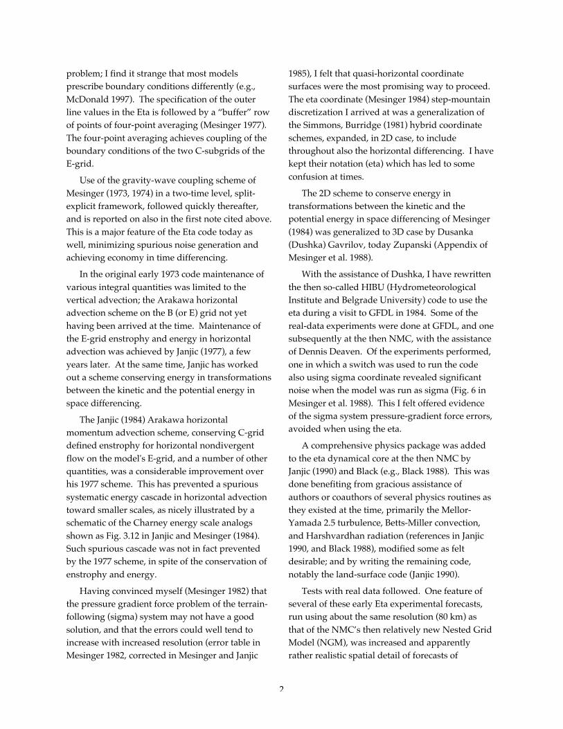
An unintended resolution/domain sizeexperiment was initiated in 1995 and was in placefor more than two years. “Meso” Eta runs wereimplemented, at 29 km/50 layer resolution, runlater so that they used current Avn boundarycondition, and also more data. To be able to affordhigher resolution the 29 km domain was chosensmaller than that of the 48 km Eta; the twodomains are shown in Fig. 3. A clear improvementwas expected.

While some forecasts and certainly local detailwere improved, as can be seen in Fig. 4 instatistical QPF sense in a two-year sample of 1245forecasts no advantage of the 29 km model overthe 48 km one was evident.

What was going on? The explanation hard toavoid is that the considerably larger domain of the48-km Eta was of so much benefit as to more than

compensate for the negative impact of its 12 h oldlateral boundary data. For this, of the three majorfactors involved, resolution, accuracy of the lateralboundary condition, and the domain size, thedomain size had to be the dominant one.

Note that this result, or explanation, is at oddswith a rather widespread view of looking at nestedmodels as “downscaling” tools, which aresupposed to provide local detail but should notchange the large scale fields of the driver model(e.g., Waldron et al. 1996; von Storch et al. 2000;Castro and Pielke 2004). The result of Fig. 4suggests that a limited area model should be, andalso indicates that it can be, able to improve notonly on the local detail but on the largest scales itcan accommodate as well. In other words,“upscaling” can take place, and it seems to me itshould, unless the nested model has problems ofsome kind. Such problems could be due to the useof the Davis-type relaxation boundary condition,given that this is a feature common to manymodels but not present in the Eta.

I will return to this point of the apparent Etastrength in largest scales the model canaccommodate at several places in the sections tofollow.

Fig. 3. The domains of the Eta 48-km and of the Eta 29-km model.

6

Fig. 4. Equitable precipitation threat scores for four of NCEP's operational models, those of preceding figures andfor the “29-km Eta” (MESO), for various precipitation thresholds, and for the period 16 October 1995 - 15 October1997, left panel; bias scores for the same models and period, right panel. “All Periods” refers to two verificationperiods, 00-24 h, and 12-36 h; note that the 29-km model was run only 33 h ahead. It was initialized 3 h later than theremaining models. The sample contains 1,245 forecasts by each of the four models; 618 of them verifying at 24 h, and627 verifying at 36 h.

4. The Eta vs the Avn/GFS

Comparing results of a nested regional modelagainst those of its driver global model, numerousquestions may come to mind. First of all, what isthe objective of running the nested model?Clearly, it must be value added, hopefullyincreased or additional skill, of some kind.Deciding what this hoped for increased skill is, onewill normally ask if is it being achieved. If it is,why is yet another question; how long can it bemaintained one more. A less ambitious goal, morein tune with the present-day thinking would be:increased skill at least some of the time.

The “dry” eta code came to NMC the very sameyear, 1984, when the daily real-time forecasts usingthe NGM (RAFS) were started. Thus, one maywonder, is there any record of what the objectiveof the NGM was thought to be? In the conferencepaper summarizing results from the first year ofreal-time forecasting Hoke et al. (1985) state thatthe NGM was implemented “with the

fundamental goal of improving operationalforecasts of heavy precipitation out to 48 hours”.

Fig. 1 has shown that the Eta in its first 24months of three-model precipitation scores wasachieving this goal comfortably, for allprecipitation thresholds, in spite of absorbing thevery real handicap of being run first, using 12-hold Avn boundary conditions, and also a shorterdata cut-off.

Even so, not a very bright future for the “early”Eta, the one run before the global model, wasexpected at the time. This was the period ofperhaps a widespread enthusiasm with the successof the European Centre, and global spectral modelsin general. Thus, the NMC Development Divisionmanagement plans of 1993 (Kalnay et al. 1993)foresee that already in October 1996 the early Etawas going to be “Phased out assuming AVNprecipitation guidance 24-48 hour is comparable orbetter.”

This did not happen. The advantage of the Eta

7

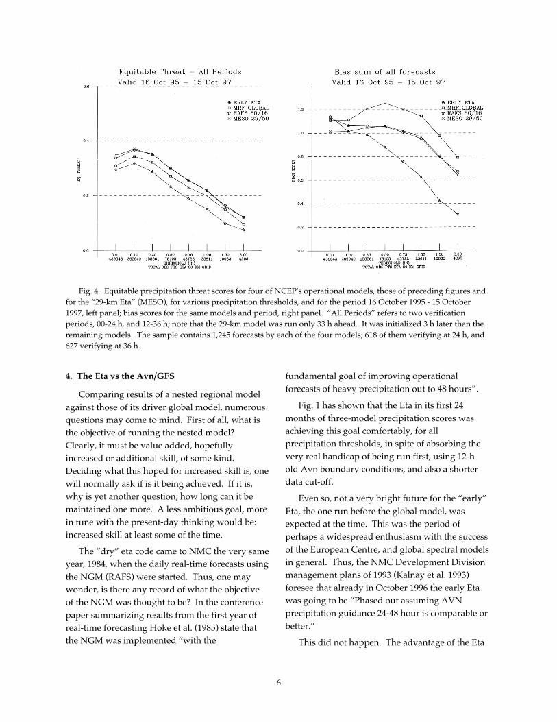
over the Avn in the second 24 months of three-model scores, September 1995-August 1997, Fig. 5,stayed about the same. Compared to the frozen

NGM, both models have clearly improved, acrossof the thresholds monitored.

Fig. 5. Same as Fig. 1, except for the 24-month period September 1995-August 1997; and for the Eta being run at48-km resolution during most of the period shown. The sample contains 1,970 verifications by each of the threemodels.

As for the Eta, a major set of model changesthat have contributed to its improvement are thoseof the upgrade implemented on 12 October 1995(Rogers et al. 1996; Mesinger 1996). These changesincluded a horizontal resolution increase, from 80to 48 km; and a small increase in the domain size,from 105° x 75 10/26° to 106° x 80° of rotatedlongitude x latitude, same as the Eta domain usedtoday.

Main model changes of October 1995 have allbeen tested separately, and convincing evidencewas obtained of the resolution increase resulting inbetter scores (Rogers et al. 1995b). Two earlierresolution experiments gave similar results (Black1994; Mesinger et al. 1997). Thus, implementationof the 29-km “Meso Eta”, now using current Avnlateral boundary condition, was a logical step. Yet,results displayed in Fig. 4, from a very largesample, show no increase in scores. The reduced

domain size, as pointed out, seems the onlycredible explanation.

But one might still wonder: is the larger domainbeneficial because of enabling the Eta to generatemore accurate larger scales, as suggested in thepreceding section, or perhaps by way of its movingthe notorious “lateral boundary error” furtheraway from the U.S. verification area?

Convincing evidence seems to exist that themathematical error of the Eta lateral boundaryscheme is not significant (e.g., Black et al. 1999).On the other hand, the rate of deterioration of skillwith forecast time is considerable and is welldocumented. Presently the operational Eta isdriven by the lateral boundary condition from theAvn (recently renamed GFS, Global ForecastingSystem) runs of 6 h ago. At the "on" times (00 and12z) this is estimated to represent about an 8 h loss

8

in accuracy. Should one then not be able to notice,as this error is advected into the central Etadomain, that the Eta skill falls behind that of theAvn/GFS at extended forecast times?

This aspect is now particularly relevant giventhat as of April 2001 the Eta forecasts have beenextended out to 84 h. Note that, just with referenceto operational LAMs being nested within low-resolution global forecast models, Laprise et al.(2000) state that "the contamination at the lateralboundaries ... limits the operational usefulness ofthe LAM beyond some forecast time range"(Laprise et al. 2000). If so, and in view of the"enhanced" contamination in case of the Eta andthe Avn/GFS, what is that time range?

This issue has already been looked into by wayof inspection of the Eta vs the Avn precipitationscores at later vs those at earlier forecast times, rmsfits to raobs as functions of time, and accuracy ofthe placement of the centers of major lows by thetwo models at 60 h forecast time (Mesinger et al.2002a; Mesinger et al. 2002b). These results will beupdated and/or recalled here.

In Fig. 6 a year, May 2001-April 2002, of the Etaand the Avn precipitation threat scores are shown,for the sample of 00-24, 12-36, and 24-48 h, upperpanel, and that of the 36-60, 48-72, and 60-84 hforecasts, all verifying at 12z, lower panel. Thereare more than 800 24-h verifications in each of thepanels. The advantage of the Eta over the Avn inthe forecast periods going beyond the two days isseen to have remained overall just about the sameas it was in the up to two day periods.

In the two cited Mesinger et al. (2002)conference papers rms fits to raobs of the Eta andthe Avn 250 mb wind and 500 mb height wereshown, as functions of forecast time, for fourseasons: spring, summer, and fall of 2001, andwinter of 2001-2002. No systematic tendency ofthe Eta error growth rate to increase relative to thatof the Avn at later forecast times was evident. Thisseries is here updated by showing in Fig. 7 250 mbwind and 500 mb height rms plots for the warmseason (May through October) of 2003, and thecold season (November through April) of 2003-

2004. An impact of the advection of the GFS lateralboundary errors is not visible in any of the fourplots shown.

As yet another attempt, the accuracy of the Etaand the Avn in placing the centers of major lows,at 60 h forecast time, during the winter of 2000-2001, was documented and reported on inMesinger at al. (2002a). Rules were set foridentification of these lows on HPC's 00 and 12zanalyses. Verification area was chosen east of theContinental Divide, to minimize the impact of thedifferences in the pressure reduction to sea level.31 cases, coming from 12 events, qualified. Resultsare reproduced in Table 1. The Eta is seen to havebeen in numerous respects considerably moreaccurate than the Avn.

With these results on major challenges,unintended experiments, and tests the Eta hasfaced or has been involved with recalled orpresented, I will now move to a more generaldiscussion: what lessons have we learned? A“lesson” of course, can also be to have a good lookinto something most of us might have been takingfor granted.

5. Discussion: Progress achieved by the Eta,order of accuracy, resolution, sigma vs eta

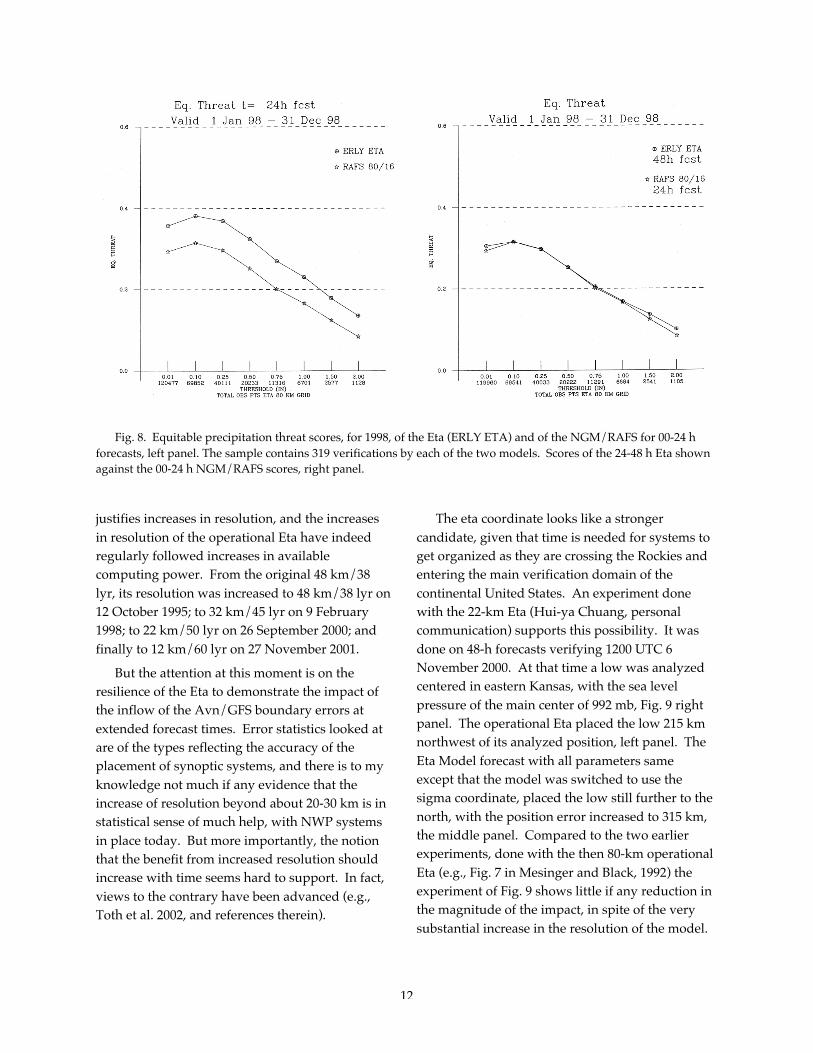
There can be little doubt that considerableprogress in NWP skill has been made during thenineties. The starting point here is to assess howmuch this is evidenced by the results of the Eta,and how much the Eta may have contributed tothis progress. NGM, frozen in 1991 and run untilFebruary 2000 with its analysis and initializationsystem also unchanged and independent of that ofthe Eta, served as a unique reference model to thatend. Thus, in the left panel of Fig. 8 equitablethreat scores are given of the Eta and the NGM(RAFS) 24 h accumulated precipitation forecastsfor all of 1998. In the right panel, the 24-h NGMthreat score plot is reproduced along with that ofthe Eta 24-48 h forecasts. For all eight categoriesthe Eta 48 h scores are higher than those of theNGM’s 24 h ones, albeit at five of them thedifference is barely visible. Thus, in seven years,

9

Fig. 6. Equitable precipitation threat scores of the Eta (solid) and the Avn (dashed lines), 00-24, 12-36, and24-48 h forecasts, upper panel, and 36-60, 48-72, and 60-84 h forecasts, lower panel, May 2001-April 2002.

10

Fig. 7. RMS fits to raobs of the operational forecasts of the Eta (solid) and of the GFS (dashed lines), in the “warmseason” of 2003 (left panels) and in the “cold season” of 2003-2004 (right panels); for 250 mb vector winds (upperpanels), and 500 mb heights (lower panels), as functions of forecast time. The Eta is verified after being output to a40-km grid (“grid 212”), and the GFS after being output to an 80-km grid (“grid 211”)

a full day extension of the validity of NCEP’s“official” QPFs has been achieved.

But how much of this progress, if any, is due tothe Eta itself, and how much merely to increasedresolution enabled by more computing power?Attempting to assess what the answer might becomparisons of Section 2 of the Eta against theNGM and the RSM come to mind, being done withmodels run at about the same resolution, andhaving physics packages of roughly similarcomplexity.

Considerable advantage of the Eta against bothof these models has been evidenced. What

message, if any, does this imply? NWP is animprecise science, in the sense that cleanexperiments are virtually impossible. Yet, ifenough evidence accumulates, and if a physicalunderstanding seems plausible, credibility of theevidence becomes hard to deny. In this respect, acommon feature of the NGM and the RSM ofhaving a higher formal (Taylor series based)accuracy compared to the 2nd-order accurate Eta isworth recalling. If higher accuracy were helpful tothe NGM and to the RSM, this help clearly was nottoo significant. The 29 km Eta of Section 3 was alsoformally more accurate than the 48 km one, andthe help, if any, was not too significant either. At

11

Table 1. Position forecast errors, at 60 h, of "major lows"east of the Rockies and over land,December 2000 - February 2001

–––––––––––––––––––––––––––––––––––––––––Valid at Avn error Eta error

00z 12 Dec. 125 km 275 km12z 12 Dec. 325 km 150 km

00z 17 Dec. 475 km 125 km12z 17 Dec. 175 km 425 km00z 18 Dec. 450 km 575 km12z 18 Dec. 75 km 100 km

00z 20 Dec. 250 km 350 km12z 20 Dec. 175 km 175 km

00z 5 Jan. 400 km 350 km12z 5 Jan. 125 km 350 km

12z 6 Jan. 1,175 km 500 km

12z 10 Jan. 325 km 150 km00z 11 Jan. 425 km 75 km

12z 13 Jan. 475 km 150 km00z 14 Jan. 50 km 350 km12z 14 Jan. 175 km 150 km00z 15 Jan. 350 km 300 km12z 15 Jan. 225 km 175 km00z 16 Jan. 225 km 275 km

00z 30 Jan. 175 km 350 km12z 30 Jan. 300 km 275 km

00z 9 Feb. 350 km 325 km

00z 10 Feb. 150 km 175 km12z 10 Feb. 225 km 200 km

12z 21 Feb. 575 km 325 km

00z 24 Feb. 325 km 100 km12z 24 Feb. 300 km 100 km00z 25 Feb. 275 km 150 km12z 25 Feb. 325 km 300 km00z 26 Feb. 475 km 75 km12z 26 Feb. 575 km 175 km

–––––––––––––––––––––––––––––––––––––––––Average error 324 km 244 kmMedian error 300 km 200 km

least one other relatively recent effort to benefitfrom higher-order differencing in a major NWPmodel has also failed to lead to increased skill.Thus, Cullen et al. (1997) state that "the sensitivityof the complete model to the choice betweensecond and fourth order schemes ... has beenslight".

I have repeatedly hypothesized earlier (e.g.,Mesinger 2001) that this could be due to theinconsistency in the treatment of dynamics and

physics in NWP models: in dynamics smoothfields are assumed, and grid point values areconsidered valid at points; in physics, noise isproduced by changing individual grid columns,and grid point values are considered to representaverages over the grid boxes. In no physicsexperiments (“test problem” of Cullen et al. 1997)benefits from higher order are universally present.Introduction of the physics “noise” in completemodels works against the Taylor series smoothnessview. This inconsistency being to a smaller degreedetrimental in the Eta due to a variety of itsArakawa-style finite-volume features, and – unlesscompact schemes are used – also due to its only2nd-order formal accuracy, could havesignificantly contributed to the Eta performance asreviewed above.

How can this conundrum be resolved? Onepossibility, making sense also from a physicalpoint of view (Arakawa 2000b) is to move awayfrom single-column parameterizations. Another isto refine numerical discretizations, so as to try toabandon completely the treatment of grid pointvalues as point samples of smooth functions.Piecewise-polynomial methods offer suchpossibilities.

The lack of evidence of the Avn (or, GFS) lateralboundary error affecting the relative skill of the Etaat extended forecast times is another issue beggingfor understanding. A number of implications canbe made. Note first that for the Eta skill relative tothe Avn not to be visibly affected by the inflow ofthe less accurate Avn/GFS boundary data beyondabout two days, component(s) are needed in theEta able to compensate for this inflow.Furthermore, the impact of this(these)component(s) ought to increase with time.

The higher Eta resolution seems a weakcandidate for this role; recall the experiment ofSection 3. Impressive benefits of high resolutionare well-known for more local events and atshorter range, such as in the notorious 10-km Etaforecast of very heavy rains over California coastalranges in February 1998 (e.g., Wu 1999). With nodeterioration of synoptic-scale skill, this alone

12

Fig. 8. Equitable precipitation threat scores, for 1998, of the Eta (ERLY ETA) and of the NGM/RAFS for 00-24 hforecasts, left panel. The sample contains 319 verifications by each of the two models. Scores of the 24-48 h Eta shownagainst the 00-24 h NGM/RAFS scores, right panel.

justifies increases in resolution, and the increasesin resolution of the operational Eta have indeedregularly followed increases in availablecomputing power. From the original 48 km/38lyr, its resolution was increased to 48 km/38 lyr on12 October 1995; to 32 km/45 lyr on 9 February1998; to 22 km/50 lyr on 26 September 2000; andfinally to 12 km/60 lyr on 27 November 2001.

But the attention at this moment is on theresilience of the Eta to demonstrate the impact ofthe inflow of the Avn/GFS boundary errors atextended forecast times. Error statistics looked atare of the types reflecting the accuracy of theplacement of synoptic systems, and there is to myknowledge not much if any evidence that theincrease of resolution beyond about 20-30 km is instatistical sense of much help, with NWP systemsin place today. But more importantly, the notionthat the benefit from increased resolution shouldincrease with time seems hard to support. In fact,views to the contrary have been advanced (e.g.,Toth et al. 2002, and references therein).

The eta coordinate looks like a strongercandidate, given that time is needed for systems toget organized as they are crossing the Rockies andentering the main verification domain of thecontinental United States. An experiment donewith the 22-km Eta (Hui-ya Chuang, personalcommunication) supports this possibility. It wasdone on 48-h forecasts verifying 1200 UTC 6November 2000. At that time a low was analyzedcentered in eastern Kansas, with the sea levelpressure of the main center of 992 mb, Fig. 9 rightpanel. The operational Eta placed the low 215 kmnorthwest of its analyzed position, left panel. TheEta Model forecast with all parameters sameexcept that the model was switched to use thesigma coordinate, placed the low still further to thenorth, with the position error increased to 315 km,the middle panel. Compared to the two earlierexperiments, done with the then 80-km operationalEta (e.g., Fig. 7 in Mesinger and Black, 1992) theexperiment of Fig. 9 shows little if any reduction inthe magnitude of the impact, in spite of the verysubstantial increase in the resolution of the model.

13

Fig. 9. The Eta Model 48 h forecasts valid 1200 UTC 6 November 2000, done using its operational eta code (leftpanel), same but run using the sigma coordinate (middle panel), and the HPC verification analysis (right panel). Theposition error of the low of the Eta forecast is 215 km, and that of the Eta sigma coordinate forecast 315 km.

There are other indications suggesting thebeneficial impact of the eta coordinate in obtaininga more realistic large-scale flow resulting from theimpact of the Rocky Mountain topography. Notethat the effect of the topographic barrier on theflow in the verification region here of mostinterest, the contiguous United States, should beexpected to be the largest in winter, because the jetstream is then furthest to the south, atpredominantly the contiguous U.S. latitudes.Inspection of rms plots such as those of Fig. 7shows that the Eta in relative terms, compared tothe Avn/GFS, does best in winter. This is just theopposite of what one might expect on account ofthe lateral boundary error propagating then intothe main verification area the fastest.

Similarly, extensive comparisons have beenmade of the accuracy of the just completed 25-yearNorth American Regional Reanalysis (RR,Mesinger et al. 2004), done using the Eta,compared to that of the NCEP/NCAR GlobalReanalysis (GR, Kalnay et al. 1996). Contrary towhat I think most people would expect on accountof the higher resolution of the Eta and thusimproved topographic and land-surface realism,

the greatest advantage of the RR over the GR isapparently in winds, in winter, at jet stream levels.

But in the late nineties, before these resultsbecame available, considerable concern had arisenas a result of a failure of a quasi-operational 10-kmEta to perform well in forecasting an intensedownslope windstorm in the lee of the Wasatchmountain (McDonald et al. 1998), while the sigmasystem MM5 for the same case did well. This wasfollowed by 2D experiments of Gallus and Klemp(2000), in which an eta code in a flow up and downa bell-shaped mountain failed to bring thestrongest winds close to the ground on the lee side,as should have occurred according to a linearsolution. Instead, a flow separation developed inthe lee of the mountain. In addition, in Gallus andKlemp (2000) various scale- and resolution-relatedarguments were made.

As a result, the eta has lost much of its originalrespect and the opinion now seems to be quitewidespread in the NWP community that the etacoordinate system is "ill suited for high resolutionprediction models" (e.g., Schär et al. 2002; Janjic2003; Steppeler et al. 2003; Mass et al. 2003; Zängl2003). Various authors expressing that view have

14

used and/or advocated sigma or modified sigmasystems. It would seem thus that it is alsoconsidered that as the resolution of NWP models isbeing increased the performance of the terrainfollowing coordinates will increasingly improve,so that an alternative rather complex system of"shaved cells" (Adcroft et al. 1999) is not cost-beneficial. Yet another option, of an eta-likesystem but with partial steps (Tripoli, personalcommunication) seems not to be attracting muchinterest. Thus, for example, all three major WRFdynamical core development efforts are based onvarious versions of the terrain-followingcoordinates.

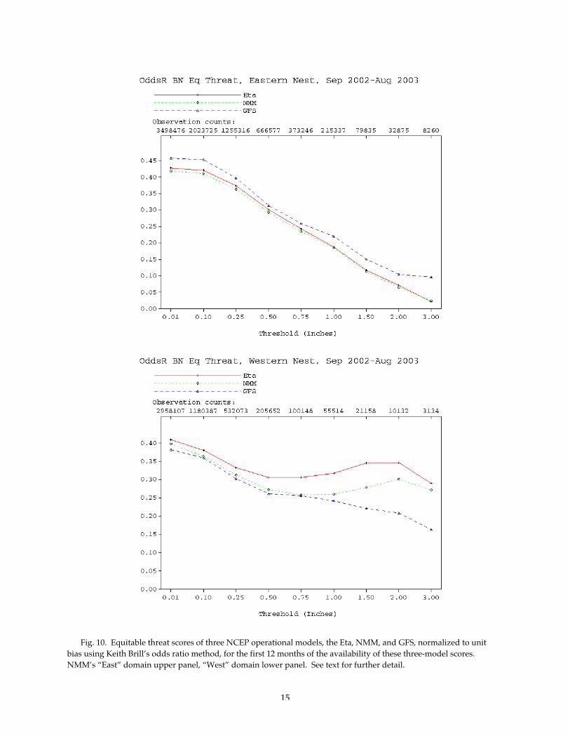
Results of the first 12 months of comparison ofprecipitation scores of three NCEP operationalmodels, Global Forecasting System (GFS), 12-kmEta, and 8-km Nonhydrostatic Mesoscale Model(NMM) are however at variance with this view.These 12 months are of particular interest sincethey have included the el Niño winter of 2002-2003, when during the November and December2002 five events are on record of very heavy rainsover the mountainous western United States withHPC analyzed precipitation of over 4 inches/24hours, and typically 2 and 3 inches/24 hourpatterns over individual mountain ranges that areclearly an extraordinary challenge to forecast wellin terms of precipitation scores. A summary ofthese 12 month results, in form of equitable threatscores normalized to unit bias using Keith Brill’sodds ratio method (Mesinger and Brill 2004) isshown in Fig. 10. These results also raiseadditional concerns regarding the expectation ofimproved skill with increased resolution. Over theroughly eastern half of the United States, with nomajor topography (“East”), the Eta and the NMMhad about the same skill; if anything, the lowerresolution Eta did slightly better. The GFS wasclearly better than the two. Over the mountainouswestern half, “West”, it was the Eta that hadclearly the best scores, with the sigma systemNMM second, and the GFS third.

How is that possible? Explanation of the etadownslope windstorm problem has been

suggested in Mesinger (2004). The problem,absence of slantwise flow between neighboring etalayers, should not much affect the performance ofthe eta on the upslope side, and therefore theperformance of the Eta for the mentioned veryheavy el Niño rains over the West was excellent,much better than that of the sigma system models,NMM and also GFS. Over the East, the impact oftopography was not dominant, and the Eta and theNMM performed similarly.

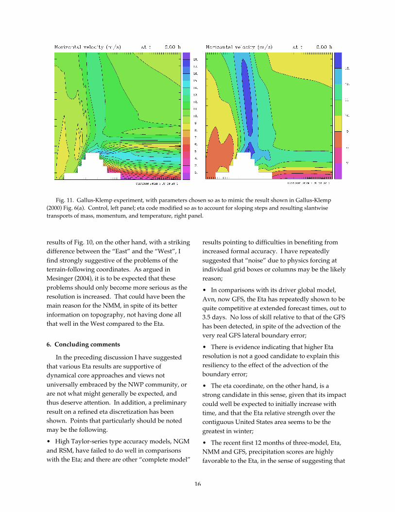
In an effort in progress (Mesinger and Jovic) wehave refined the eta code so as to account forslopes replacing the flat tops of the current step-topography Eta discretization. Accordingly, theeta vertical velocity next to the ground is notrequired to be zero. Of the eta governingequations, this affects only the pressure tendencyequation (Mesinger 2000b). With our currentapproach, topography slopes are defined atvelocity points, and are defined at squaresbounded by four neighboring height points. Apreliminary result we have with this approach atthe time of this writing is shown in Fig. 11. Its leftpanel shows our emulation of the Gallus-Klempexperiment, their Fig. 6(a). We have obtained thisresult using a full 3D Eta code, dynamics only,running a square domain, with variablesprescribed not to change along one of itsdiagonals. Flow separation in the lee as seen inthis panel was considered by Gallus and Klempillustration of the Eta downslope windstormproblem; just as in their plot, a velocity of onlybetween 1 and 2 m/s is seen in our left panel plotimmediately behind the obstacle next to theground. In the right panel, obtained using oursloping steps discretization, an add-on to thecurrent eta code, a considerably greater velocity isseen next to the ground just behind the obstacle, ofbetween 7 and 8 m/s. In addition, the noisycontour pattern at the upslope side is replaced by aconsiderably smoother pattern.

I consider this very preliminary result ademonstration that the eta downslope windstormproblem should not be too hard to remedy by anadd-on to the current eta code. The precipitation

15

Fig. 10. Equitable threat scores of three NCEP operational models, the Eta, NMM, and GFS, normalized to unitbias using Keith Brill’s odds ratio method, for the first 12 months of the availability of these three-model scores.NMM’s “East” domain upper panel, “West” domain lower panel. See text for further detail.

16

Fig. 11. Gallus-Klemp experiment, with parameters chosen so as to mimic the result shown in Gallus-Klemp(2000) Fig. 6(a). Control, left panel; eta code modified so as to account for sloping steps and resulting slantwisetransports of mass, momentum, and temperature, right panel.

results of Fig. 10, on the other hand, with a strikingdifference between the “East” and the “West”, Ifind strongly suggestive of the problems of theterrain-following coordinates. As argued inMesinger (2004), it is to be expected that theseproblems should only become more serious as theresolution is increased. That could have been themain reason for the NMM, in spite of its betterinformation on topography, not having done allthat well in the West compared to the Eta.

6. Concluding comments

In the preceding discussion I have suggestedthat various Eta results are supportive ofdynamical core approaches and views notuniversally embraced by the NWP community, orare not what might generally be expected, andthus deserve attention. In addition, a preliminaryresult on a refined eta discretization has beenshown. Points that particularly should be notedmay be the following.• High Taylor-series type accuracy models, NGMand RSM, have failed to do well in comparisonswith the Eta; and there are other “complete model”

results pointing to difficulties in benefiting fromincreased formal accuracy. I have repeatedlysuggested that “noise” due to physics forcing atindividual grid boxes or columns may be the likelyreason;• In comparisons with its driver global model,Avn, now GFS, the Eta has repeatedly shown to bequite competitive at extended forecast times, out to3.5 days. No loss of skill relative to that of the GFShas been detected, in spite of the advection of thevery real GFS lateral boundary error;• There is evidence indicating that higher Etaresolution is not a good candidate to explain thisresiliency to the effect of the advection of theboundary error;• The eta coordinate, on the other hand, is astrong candidate in this sense, given that its impactcould well be expected to initially increase withtime, and that the Eta relative strength over thecontiguous United States area seems to be thegreatest in winter;• The recent first 12 months of three-model, Eta,NMM and GFS, precipitation scores are highlyfavorable to the Eta, in the sense of suggesting that

17

the benefit from its vertical coordinate in events ofvery strong precipitation in the “West” wassufficient to overcome the handicaps of oldboundary conditions compared to the GFS, andless information on complex topographycompared to the higher resolution NMM;• This is strongly indicative of the sigma systempressure gradient force problem not beingalleviated with increased resolution, but insteadthe opposite taking place, as argued in Mesinger(2004) and earlier one should expect. Recall that ofthe numerous attempts to address the problem, asreviewed in Mesinger and Janjic (1985), none reallyremove it;• The Eta problem with downslope windstormsas evidenced by the Gallus-Klemp experiment, onthe other hand, seems not hard to successfullyaddress. The emulation of the Gallus-Klempexperiment shown here along with a preliminaryresult obtained using a refined eta discretization,an add-on to the current Eta code, is not far from ademonstration that this in fact had already beendone.

Acknowledgements. The “dry” eta code came tothe then NMC as a result of an NMC/GFDLcooperation effort, put in place by the directors ofthe two institutions, for which as I understand BillBonner, then NMC Director, was the driving force.The code and the associated message were clearlywell received, not only by Bill who did his best tomake my one-year visit pleasant as well as useful;but by the then Development Division staff just aswell. This being an appropriate opportunity, Ihave asked Tom Black, who in a way took overlooking after the code at NMC [and very early puttogether this wonderful model documentation, stillindispensable, Black (1988)], to recollect the eventsfollowing my one year visit 1984-1985. I’ll quotethe main body of Tom’s reply:

“Here is what I can say about Ron [McPherson]as well as Joe Gerrity in the early days givenmy less than stellar memory. … I assume thatthe work you had done with Dennis Deaven

and others with the "dry" version of the Eta (thematerial for the '88 paper) had sufficientlyimpressed Ron that he definitely wanted topursue its development. I don't rememberexactly what Ron had to say but I believe thathe already knew I was enthusiastic about themodel ever since you gave a seminar in 209 onthe pressure gradient problem in '85 or '86 so assoon as I finished my postdoc and was hired byNMC, he asked me to look into incorporatingthe GFDL physics into the model since the lackof physics was the glaring inadequacy at thattime. Of course that effort was set aside whenZavisa [Janjic] brought Betts and Mellor-Yamada. As on offshoot of Ron's asking me todo that, I know it wasn't too long after going upto Princeton that I was showing something at abranch meeting about that GFDL code when Ikept referring to it as the eta model since I wasused to referring to a model by its verticalcoordinate (I called the model used for my PhDwork at Wisconsin the isentropic model). … Iassume everyone else soon started using thatname too solely due to its simplicity as opposedto using HIBU or step mountain for the name.Probably not long after that time Joe asked(told) me to write a documentation of themodel since no one other than you or Zavisawas at all familiar with it; to me this stronglyindicates that he was a supporter too. I knowJoe liked all the finite difference equations I putinto that documentation; he enjoyed checkingthem for symmetry and he subsequentlyvolunteered to type up the entire documentsince we didn't have workstations yet. I got thedefinite impression he was eager to learn abouthow the model worked. After that thingsseemed to just flow naturally as I helped youand Zavisa so I have no other pivotal memoriesof other contributors before Eugenia announcedthat the Eta was going to replace the LFM.”

Going now on just briefly beyond the earliestNMC times, results shown here obtained using theEta were made possible only due to efforts ofnumerous people who have contributed to thedesign of the model, some by generouslyproviding codes as mentioned in Section 1, and yetothers by developing the model’s data assimilation

18

system; and last but definitely not least, keptseeing to it that various systems are maintained.Tom Black and Eric Rogers, overseeing the smoothoperation of the system during about a decade anda half addressed, should particularly bementioned. The beginnings of the EMCprecipitation verification system have been put inplace by John Ward, the system was then furtherdeveloped and maintained by Mike Baldwin, andfor quite a few years now is developed still moreand maintained by Ying Lin. Various scores aswell as rms plots shown were obtained using theNCEP forecast verification system maintained byKeith Brill. And last but once again not least,enthusiastic support of Eugenia Kalnay, head ofthe NMC Development Division in charge of theoperational implementation of the Eta in 1993,should be recalled.

REFERENCES

Adcroft, A., C. Hill, and J. Marshall, 1997:Representation of topography by shaved cells in aheight coordinate ocean model. Mon. Wea. Rev., 125,2293-2315.

Arakawa, A., 2000a: A personal perspective on the earlyyears of general circulation modeling at UCLA.General Circulation Model Development: Past, Presentand Future. D. A. Randall, Ed., Academic Press, 1-65.

Arakawa, A., 2000b: Future development of generalcirculation models. General Circulation ModelDevelopment: Past, Present and Future. D. A. Randall,Ed., Academic Press, 721-780.

Black, T. L., 1988: The step-mountain eta coordinate regionalmodel: A documentation. NOAA/NWS NationalMeteorological Center, April 1988, 47 pp. [Availablefrom NOAA Environmental Modeling Center, Room207, 5200 Auth Road, Camp Springs, MD 20746.]

Black, T. L., 1994: The new NMC mesoscale Eta Model:Description and forecast examples. Wea. Forecasting,9, 265-278.

Black, T. L., and Z. I. Janjic, 1988: Preliminary forecastresults from a step-mountain eta coordinate regionalmodel. Preprints, 8th Conf. on Numerical WeatherPrediction, Baltimore, MD, Amer. Meteor. Soc., 442-447.

Black, T. L., G. J. DiMego, and F. Mesinger, 1999: A testof the Eta lateral boundary conditions scheme. Res.

Activ. Atmos. Oc. Modelling, WMO, Geneva, CAS/JSCWGNE Rep. 28, 5.9-5.10.

Castro, C. L., and R. A. Pielke, Sr., 2004: Dynamicaldownscaling: Assessment of value added using theRegional Atmospheric Modeling System (RAMS). J.Geophys. Res. - Atmospheres, (in press).

Cullen, M. J. P., T. Davies, M. H. Mawson, J. A. James,and S. C. Coulter, 1997: An overview of numericalmethods for the next generation U.K. NWP andclimate model. Numerical Methods in Atmospheric andOceanic Modelling, C. Lin, R. Laprise, and H. Ritchie,Eds. The André J. Robert Memorial Volume.Canadian Meteorological and OceanographicSociety/NRC Research Press. 425-444.

Gallus, W. A., Jr., and J. B. Klemp, 2000: Behavior offlow over step orography. Mon. Wea. Rev., 128, 1153-1164.

Hoke, J. E., N. A. Phillips, G. J. DiMego, and D. G.Deaven, 1985: NMC's Regional Analysis andForecast System - results from the first year of daily,real-time forecasting. Preprints, 7th Conf. onNumerical Weather Prediction, Montreal, P.Q., Canada,Amer. Meteor. Soc., 444-451.

Janjic, Z. I., 1977: Pressure gradient force and advectionscheme used for forecasting with steep and smallscale topography. Contrib. Atmos. Phys., 50, 186-199.

Janjic, Z. I., 1984: Nonlinear advection schemes andenergy cascade on semi-staggered grids. Mon. Wea.Rev., 112, 1234-1245.

Janjic, Z. I., 1990: The step-mountain coordinate:physical package. Mon. Wea. Rev., 118, 1429-1443.

Janjic, Z. I., 1994: The step-mountain eta coordinatemodel: Further developments of the convection,viscous sublayer, and turbulence closure schemes.Mon. Wea. Rev., 122, 927-945.

Janjic, Z. I., 2003: A nonhydrostatic model based on anew approach. Meteor. Atmos. Phys., 82, 271-301.

Janjic, Z. I., and F. Mesinger, 1984: Finite-differencemethods for the shallow water equations on varioushorizontal grids. Numerical Methods for WeatherPrediction, Vol. 1, Seminar 1983, ECMWF, Reading,UK, 29-101.

Juang, H.-M. H., S.-Y. Hong, and M. Kanamitsu, 1997:The NCEP regional spectral model: An update. Bull.Amer. Meteor. Soc., 78, 2125-2143.

Kalnay, E., W. Baker, M. Kanamitsu, R. Petersen, D. B.Rao, and A. Leetmaa, 1993: Modeling plans at NMCfor 1993-1997. 13th Conf. on Weather Analysis andForecasting, Vienna, VA, Amer. Meteor. Soc., 340-343.

19

Kalnay, E., and Coauthors, 1996: The NCEP/NCAR 40-Year Reanalysis Project. Bull. Amer. Meteor. Soc., 77,437-471.

Laprise, R., M. R. Varma, B. Denis, D. Caya, and I.Zawadzki, 2000: Predictability of a nested limited-area model. Mon. Wea. Rev., 128, 4149-4154.

Mass, C. F., and Coauthors, 2003: Regionalenvironmental prediction over the Pacific Northwest.Bull. Amer. Meteor. Soc., 84, 1353-1366.

McDonald, A, 1997: Lateral boundary conditions foroperational regional forecast models; a review. HIRLAMTech. Rep. 32, 32 pp. [Available from A. McDonald,Irish Meteorological Service, Glasnevin Hill, Dublin9, Ireland.]

McDonald, B. E., J. D. Horel, C. J. Stiff, and W. J.Steenburgh, 1998: Observations and simulations ofthree downslope wind events over the northernWasatch Mountains. Preprints, 16th Conf. on WeatherAnalysis and Forecasting, Phoenix, AZ, Amer. Meteor.Soc., 62-64.

Mesinger, F., 1973: A method for construction ofsecond-order accuracy difference schemespermitting no false two-grid-interval wave in theheight field. Tellus, 25, 444-458.

Mesinger, F., 1974: An economical explicit schemewhich inherently prevents the false two-grid-intervalwave in the forecast fields. Proc. Symp. "Differenceand Spectral Methods for Atmosphere and OceanDynamics Problems", Academy of Sciences,Novosibirsk 1973; Part II, 18-34.

Mesinger, F., 1977: Forward-backward scheme, and itsuse in a limited area model. Contrib. Atmos. Phys.,50, 200-210.

Mesinger, F., 1982: On the convergence and errorproblems of the calculation of the pressure gradientforce in sigma coordinate models. Geophys.Astrophys. Fluid. Dyn., 19, 105-117.

Mesinger, F., 1984: A blocking technique forrepresentation of mountains in atmospheric models.Riv. Meteor. Aeronautica, 44, 195-202.

Mesinger, F., 2000a: Numerical methods: The Arakawaapproach, horizontal grid, global, and limited-areamodeling. General Circulation Model Development:Past, Present and Future. A. Randall, Ed., AcademicPress, 373-419.

Mesinger, F., 2000b: The sigma vs eta issue. Res. Activ.Atmos. Oc. Modelling, WMO, Geneva, CAS/JSCWGNE Rep. 30, 3.11-3.12.

Mesinger, F., 2001: Limited area modeling: Beginnings,state of the art, outlook. 50th Anniversary ofNumerical Weather Prediction, Potsdam, 9-10 March

2000, Book of Lectures. A. Spekat, Ed., Europ.Meteor. Soc, 85-112. [Available from the Amer.Meteor. Soc.]

Mesinger, F., 2004: The steepness limit to validity ofapproximation to pressure gradient force: Any signsof an impact? 20th Conf. on Weather Analysis andForecasting/16th Conference on Numerical WeatherPrediction, paper P1.19, Combined Preprints CD-ROM, 84th AMS Annual Meeting, Seattle, WA.

Mesinger, F., and T. L. Black, 1992: On the impact onforecast accuracy of the step-mountain (eta) vs.sigma coordinate. Meteor. Atmos. Phys., 50, 47-60.

Mesinger, F., and K. Brill, 2004: Bias normalizedprecipitation scores. 17th Conf. on Probability andStatistics in the Atmospheric Sciences, paper J12.6,Combined Preprints CD-ROM, 84th AMS AnnualMeeting, Seattle, WA.

Mesinger, F., and Z. I. Janjic, 1974: Noise due to time-dependent boundary conditions in limited areamodels. The GARP Programme on NumericalExperimentation, Rep. 4, WMO, Geneva, 31-32.

Mesinger, F., and Z. I. Janjic, 1985: Problems andnumerical methods of the incorporation ofmountains in atmospheric models. Large-scaleComputations in Fluid Mechanics, Part 2. Lect. Appl.Math., Vol. 22, Amer. Math. Soc., 81-120.

Mesinger, F., and L. Lobocki, 1991: Sensitivity to theparameterization of surface fluxes in NMC's etamodel. Preprints, 9th Conf. on Numerical WeatherPrediction, Denver, CO, Amer. Meteor. Soc., 213-216.

Mesinger, F., Z. I. Janjic, S. Nickovic, D. Gavrilov, and D.G. Deaven, 1988: The step-mountain coordinate:Model description and performance for cases ofAlpine lee cyclogenesis and for a case of anAppalachian redevelopment. Mon. Wea. Rev., 116,1493-1518.

Mesinger, F., T. L. Black, and M. E. Baldwin, 1997:Impact of resolution and of the eta coordinate onskill of the Eta Model precipitation forecasts.Numerical Methods in Atmospheric and OceanicModelling. C. Lin, R. Laprise, and H. Ritchie, Eds. TheAndré J. Robert Memorial Volume. CanadianMeteorological and Oceanographic Society/NRCResearch Press. 399-423.

Mesinger, F., K. Brill, H.-Y. Chuang, G. DiMego, and E.Rogers, 2002a: Limited area predictability: Whatskill additional to that of the global model can beachieved, and for how long? Preprints, Symp. onObservations, Data Assimilation, and ProbabilisticPrediction, Orlando, FL, Amer. Meteor. Soc., J36-J41.

20

Mesinger, F., T. Black, K. Brill, H.-Y. Chuang, G.DiMego, and E. Rogers, 2002b: A decade+ of the Etaperformance, including that beyond two days: Anylessons for the road ahead? Preprints, 19th Conf. onWeather Analysis and Forecasting/15th Conf. onNumerical Weather Prediction, San Antonio, TX, Amer.Meteor. Soc., 387-390.

Mesinger, F., G. DiMego, E. Kalnay, P. Shafran, W.Ebisuzaki, D. Jovic, J. Woollen, K. Mitchell, E.Rogers, M. Ek, Y. Fan, R. Grumbine, W. Higgins, H.Li, Y. Lin, G. Manikin, D. Parrish, and W. Shi, 2004:North American Regional Reanalysis. 15th Symp. onGlobal Change and Climate Variations, paper P1.1,Combined Preprints CD-ROM, 84th AMS AnnualMeeting, Seattle, WA.

NWS, 1973: Numerical Weather Prediction Activities:National Meteorological Center, First Half 1973. U.S.Dept. of Commerce, NOAA, National WeatherService, Silver Spring, MD, 36 pp.

Rogers, E., D. G. Deaven, and G. J. DiMego, 1995: Theregional analysis system for the operational "early"Eta Model. Wea. Forecasting, 10, 810-825.

Rogers, E., T. L. Black, D. G. Deaven, G. J. DiMego, Q.Zhao, M. Baldwin, N. W. Junker, and Y. Lin, 1996:Changes to the operational "Early" Eta analysis/forecast system at the National Centers forEnvironmental Prediction. Wea. Forecasting, 11, 319-413.

Schär, C., D. Leuenberger, O. Fuhrer, D. Lüthi, and C.Girard, 2002: A new terrain-following verticalcoordinate formulation for atmospheric predictionmodels. Mon. Wea. Rev., 130, 2459-2480.

Simmons, A. J., and D. M. Burridge, 1981: An energyand angular-momentum conserving vertical finite-difference scheme and hybrid vertical coordinates.Mon. Wea. Rev., 109, 758-766.

Steppeler, J., R. Hess, U. Schättler, and L. Bonaventura,2003: Review of numerical methods fornonhydrostatic weather prediction models. Meteor.Atmos. Phys., 82, 287-301.

Toth, Z., Y. Zhu, I. Szunyogh, M. Iredell, and R. Wobus,2002: Does increased model resolution enhancepredictability? Preprints, Symp. on Observations, DataAssimilation, and Probabilistic Prediction, Orlando, FL,Amer. Meteor. Soc., J18-J23.

von Storch, H., H. Langenberg, and F. Feser, 2000: Aspectral nudging technique for dynamicaldownscaling purposes. Mon. Wea. Rev., 128,3664–3673.

Waldron, K. M., J. Paegle, and J. D. Horel, 1996:Sensitivity of a spectrally filtered and nudged

limited-area model to outer model options. Mon.Wea. Rev., 124, 529-547.

Wu, C., 1999: Budget boosts information technology.Science News, 155, 87.

Zängl, G., 2003: A generalized sigma-coordinate systemfor the MM5. Mon. Wea. Rev., 131, 2875–2884.