Embed Size (px)
Citation preview
The effects of unconventional monetary policyin the euro area
Adam ElbourneKan JiSem Duijndam
CPB Discussion Paper | 371

The effects of unconventional monetary policyin the euro area
Adam Elbourne, Kan Ji and Sem Duijndam
January 24, 2018
Abstract
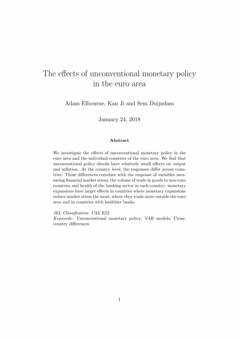
We investigate the effects of unconventional monetary policy in theeuro area and the individual countries of the euro area. We find thatunconventional policy shocks have relatively small effects on outputand inflation. At the country level, the responses differ across coun-tries. Those differences correlate with the response of variables mea-suring financial market stress, the volume of trade in goods to non-eurocountries and health of the banking sector in each country: monetaryexpansions have larger effects in countries where monetary expansionsreduce market stress the most, where they trade more outside the euroarea and in countries with healthier banks.
JEL Classification: C32; E52Keywords: Unconventional monetary policy; VAR models; Cross-country differences
1

1 Introduction
Since shortly after the fall of Lehmann Brothers the conventional instrumentof monetary policy, the short-term policy rate, has been at or close to thezero lower bound across the developed world. As such, central banks havebeen forced into conducting monetary policy through unconventional means,primarily using the quantity of assets on their balance sheets. In theory thereare a number of channels through which unconventional monetary policy canaffect the real economy (see Andrade et al. [2016] or Haldane et al. [2016]for more details), but the magnitude of those effects in the real world is anempirical question. As yet, there are only a handful of empirical studiesthat have investigated the effects of unconventional monetary policy (UMP)on output and inflation in the euro area. As our review of this literaturein Section 2 shows, most studies find that expansionary UMP does increaseoutput and inflation by a relatively small amount. This paper adds to thisrelatively scarce literature and, by also looking at the effects of UMP shocksin the individual countries of the euro area, we aim to shed some light on themost important transmission mechanisms.
A key contribution of this paper is to argue that most of the existingempirical studies of the transmission of UMP shocks are likely biased becausethey use the size of the central banks’ balance sheet directly. Balance sheetpolicies are typically announced in advance for a given period of time: forexample the Asset Purchase Programme (APP) of the ECB was unveiledin January 2015 when it was announced that AC60bn of assets would bepurchased each month until at least September 2016. As Hansen and Sargent[1991] show, this information structure leads to biased estimates (see alsoLeeper et al. [2013] for an empirical study of the effect of this informationstructure on estimates of the effects of fiscal policy). Instead, in this paper,we employ a shadow short-rate (from Wu and Xia [2016]), which is derivedfrom market bond rates. Under the assumption of efficient markets, bondrates reflect all currently available information about the future size of thebalance sheet. As such, news about future changes to the ECB’s balancesheet immediately affects the shadow rate.
We find weak evidence that expansionary unconventional monetary policyshocks increase output growth, but the effects on inflation at the aggregateeuro area level are economically insignificant. At the individual countrylevel we find a range of responses across the countries in our sample, andthose differences in the magnitudes of output responses are most consistent
2
with the liquidity premium channel, the confidence/uncertainty channel and the exchange rate channel for the transmission of unconventional monetary policy.1 We also find that larger peak output responses are associated with healthier banking systems at the start of our sample and lower government debts.
The remainder of this paper is as follows. Section 2 briefly describes the existing literature on estimating the effects of unconventional monetary pol-icy in Europe. Section 3 describes our modelling approach for the euro area level models and presents the results. Section 4 describes our country level models and attempts to explain the observed differences between countries. Finally, Section 5 offers some concluding comments.
2 Empirical evidence on unconventional mon-
etary policy in the euro area
The literature on the effects of unconventional monetary policy on the realeconomy in the euro area is not extensive. As Borio and Zabai [2016] report,there have been considerably more studies undertaken for the US and forthe effects of unconventional monetary policy on financial markets. Whenthe effects on financial markets are studied, expansionary policy in the euroarea is consistently found to lower long-term yields, reduce spreads and raiseequity prices (for example, see Beirne et al. [2011] or Baumeister and Benati[2013] for yields and spreads and Haitsma et al. [2016] for equity). Whetherthese financial market effects are transmitted through to the real economy isanother question. After all, central banks have undertaken unconventionalmonetary policy because of the deep recession caused by the financial crisesthat started with the Great Financial Crisis of 2008. In normal times bankspass on financial market developments to the real economy through theirlending decisions via a number of transmission channels (see Mishkin [1996]).It is not unreasonable to ask if the transmission of liquidity from financialmarkets to the real economy has been impaired or amplified because of theweaknesses of banks in many euro area countries since 2008.
1Following the classification of Haldane et al. [2016].
3
2.1 Shadow rates vs total assets
Empirical studies that examine the effects of unconventional monetary policyon the real economy are faced immediately with a problem: how to measurechanges in monetary policy since interest rates have been stuck at the zerolower bound? Traditional time series models used a short-term interbankrate as the instrument of monetary policy, such as the overnight EONIArate.2 As Figure 1 shows, the EONIA rate has varied little since 2009 despitelarge changes in monetary conditions as a result of unconventional monetarypolicy, which can clearly be seen in the size of the ECB’s blanace sheet. Anumber of studies have employed changes in the size of central banks’ balancesheets directly to measure monetary policy (for example Boeckx et al. [2017],Burriel and Galesi [2016], Haldane et al. [2016] or Gambacorta et al. [2014]).However, this is not without problems, since many of those changes were an-nounced some time in advance. For example, when the ECB announced QEin January 2015 it announced that AC60bn of assets would be purchased eachmonth until at least September 2016. Therefore, the balance sheet changesin the months following the January announcement were highly predictablein advance to agents in the real economy. This structure to the informationavailable to agents creates an equilibrium with a non-fundamental movingaverage representation (Hansen and Sargent [1991]). Failing to take this intoaccunt in a VAR framework leads to biased estimates of the effects of policy.In fact, this is essentially the same problem as the fiscal foresight problemin empirical analyses of the effects of fiscal policy (Leeper et al. [2013]) andis driven by the information set of the econometric model differing signif-icantly from the information set of economic agents in the economy underinvestigation.
An alternative approach to using the balance sheet directly is to use fi-nancial market prices to infer an indicator for the stance of monetary policy.Since financial market prices adjust immediately to any new information thechanges observed in these measures reflect only new information and there-fore new shocks. As such, using these prices as the measure of monetarypolicy does not suffer from the foresight problem in the way that using thebalance sheet does. The main alternative to using the central banks’ bal-ance sheet directly is to use a shadow short-rate as proposed by Wu and Xia
2The assumption behind using an interbank rate rather than the policy rate was that,whilst the central bank moved the policy rate in discrete steps, by signalling informationabout the future path of the policy rate the central bank could steer interbank rates, whichreflect all currently available information about the future direction of the policy rate.
4

Figure 1: Measures of monetary policy since 2007
0
500
1000
1500
2000
2500
3000
3500
4000
‐8
‐6
‐4
‐2
0
2
4
6
2007 2008 2009 2010 2011 2012 2013 2014 2015 2016
ECB assets (€
billion
)
Interest ra
te (%
)
Total Assets Krippner Wu and Xia EONIA
Note: The dashed vertical lines denote key UMP announcements.
[2016] and Krippner [2015b].3 Figure 1 also shows the shadow short-ratesof Wu and Xia and Krippner for the euro area. In contrast to the EONIArate, these rates show considerable movement during the zero lower boundperiod. Both of these shadow rates are calculated as a decomposition of theobserved yield curve into a shadow yield curve plus an option which pays outcash following Black [1995]. The shadow short-rate is the interest rate at theshort-term end of the shadow yield curve (see Wu and Xia [2016], Krippner[2015b] or Damjanovic and Masten [2016] for more details).
The difference between the two shadow rates concerns their estimation:the Wu and Xia measure has one fewer constraint on the empirical specifi-cation than the Krippner measure (Krippner [2015a]). This gives rise to atrade-off between letting the data speak and the risk of overfitting the data.
3More recent research has proposed estimating shadow short-rates with a time varyinglower bound for interest rates. See Lemke and Vladu [2017] for more details.
5

Krippner [2015a] argues convincingly that for the US, the more restrictedspecification leads to a better measure of the stance of monetary because keyunconventional monetary policy announcements are followed by his shadowrate moving in the direction that would be expected a priori. We follow thisprocedure for the euro area and we argue that the Wu and Xia [2016] mea-sure better tracks our a priori beliefs about the significant monetary eventsin our sample. One of the key episodes in our sample is the announcementand implementation of the APP in January 2015 (announcement) and March2015 (first purchases). In the following months the Krippner shadow rate in-dicates an almost 200 basis points tightening of monetary policy, which weview as implausible. In contrast, the Wu and Xia rate indicates a significanteasing of monetary conditions in this period. As such, for the euro area weargue that the Wu and Xia shadow rate is the better measure of the stanceof monetary policy.4
2.2 Euro area evidence
Despite the bias introduced by foresight most studies of the effects of UMPon output and prices in the euro area employ the size of ECB’s balancesheet as the measure of the stance of monetary policy. The first paper to dothis was Gambacorta et al. [2014]. They used a panel of countries for thesample period 2008 to 2011 and found significant expansionary effects froman increase in central bank’s balance sheets: increasing the balance sheet by3% increased euro area output by between 0.06% and 0.15% and increasedprices by between 0.06% and 0.11%. However, much of what we considerunconventional monetary policy has taken place after the sample period ofGambacorta et al. [2014] ended. Therefore many of the more unconventionalmonetary policies, including QE, are excluded from their analysis.
More recent papers focusing on the euro area and employing the size ofthe ECB’s balance sheet are Boeckx et al. [2017], Burriel and Galesi [2016],Haldane et al. [2016], Gambetti and Musso [2017] and Wieladek and Gar-cia Pascual [2016]. Boeckx et al. [2017] use a SVAR model identified with acombination of zero and sign restrictions for the period from 2007 to 2014 andmeasure unconventional monetary policy by the total assets on the ECB’sbalance sheet. They identify changes in policy by looking at the signs ofthe responses to changes in the assets of the ECB. They find that a 1.5%
4It has been reported by Damjanovic and Masten [2016] that this choice can make asignificant difference for estimates of the effects of unconventional monetary policy shocks.
6
increase in the size of the ECB’s balance sheet increases both output andprices by about 0.1%. Burriel and Galesi [2016] use a global VAR model forthe countries of the euro area and focus on the balance sheet of the ECB astheir measure of monetary policy (they do also report some results using theWu and Xia shadow rate instead of the size of the balance sheet, see below).The estimates of Burriel and Galesi [2016] may suffer from misspecificationbecause they specify their models using the yearly growth rates of outputand prices but do not take account of the moving average process this in-troduces into the residuals. Even so, their results at the euro area level alsohave a similar magnitude to other studies: 1% faster growth of ECB assetsis followed by a peak output growth response of almost 0.1% and inflation0.05% higher.
Haldane et al. [2016] report results from four different schemes for identi-fying unconventional monetary policy shocks based on the total assets heldon the balance sheet for a number of central banks, including the ECB, forthe period 2009 to 2015. Their results for the euro area often have the wrongsign compared to what theory would predict and none of their results arestatistically significant. Following this, Wieladek and Garcia Pascual [2016]use the same models as Haldane et al. [2016] but estimate them on datafor the period 2012 to 2016. Over this sample period their results are sta-tistically significant and the response to a 1% asset purchase shock in theeuro area is to raise output by between 0.07% and 0.15%, depending on themodel used. The magnitude of the price level results are similar with peakresponses between 0.05% and 0.1%.
Wieladek and Garcia Pascual [2016] also use their models to investigatethrough which transmission channels UMP works. They argue in favour ofthe portfolio balance channel because they observe significant responses oflong-term government bond yields and they interpret movements in futuresrates following a UMP shock as evidence in favour of the signalling channel.They also find evidence in favour of the exchange rate channel.
Whilst the papers described above are concerned with UMP in general,Gambetti and Musso [2017] focus on the effects of the announcement of theAPP in January 2015. They employ a time varying parameters VAR modelwith the unexpected component of the APP announcement identified throughsign and zero restrictions combined with a restriction on the magnitude of thechange in the ECB’s balance sheet. They find that the APP shock initiallyhad a larger effect on output than inflation before the effect of the APP shockon inflation increased significantly over the medium term.
7

To our knowledge, the only papers to use a shadow short-rate instead of thesize of the ECB’s balance sheet are Burriel and Galesi [2016] and Damjanovicand Masten [2016]. Burriel and Galesi [2016] report that a 25 basis pointsreduction in the shadow rate increases output growth by up to 2.5% andinflation by 0.1%, although as with their balance sheet based VAR modeldescribed above these results also come from a model that does not take intoaccount the moving average process that modelling yearly growth rates ofoutput and prices introduces. Damjanovic and Masten [2016] use a simplethree variable VAR model with output, prices and the shadow short-rate ofKrippner as the measure of unconventional monetary policy. They reportthat an unconventional monetary policy shock that raises the shadow rateby 100 basis points lowers euro area output by about 0.7% and lowers pricesby about 0.2%.
2.3 Country level evidence
These papers also report the effects on individual euro area countries. Forexample, Boeckx et al. [2017] report significant variation in output responsesacross euro area countries, with crisis countries having small or even negativeresponses to expansionary unconventional monetary policy shocks and non-crisis having significantly larger responses. Interestingly, they report that theNetherlands has almost no output response at all. Boeckx et al. [2017] ex-plain the cross country differences by noting the high correlation between thepeak output response and bank capital ratios: countries with well capitalisedbanks have experienced larger output effects from expansionary unconven-tional monetary policy shocks.
The finding that bank capital explains the cross-country differences intransmission is shared by Burriel and Galesi [2016]. They find that the crisiscountries of Greece, Spain, Portugal and Cyprus are in the group with thesmallest output responses to expansionary unconventional monetary policyshocks. Once again, the Netherlands is more similar to this group thanto those that have the largest responses. Given the similarity of the crosscountry differences to those reported by Boeckx et al. [2017] it should comeas no surprise that the most important factor for explaining the differencesis once again bank capital.
Wieladek and Garcia Pascual [2016] also look at some of the membercountries of the euro area with the same four identification schemes they
8

also used at the euro area level. Of the five countries they report results for,Italy always has the smallest peak output response and Spain always hasthe largest response to an unconventional monetary policy shock. France,Germany and Portugal are similar to each other and are between Italy andSpain. Wieladek and Garcia Pascual [2016] argue that the cross countrydifferences are linked to their mortgage finance systems: Spain has a highmortgage to GDP ratio and a lot of floating rate mortgage debt (95% ofmortgage debt in Spain is linked to the 12 month euribor rate), whilst at theother end Italy has a very low share of mortgages to GDP.
Whilst not including such a broad set of countries, Damjanovic and Masten[2016] do compare the effects of unconventional monetary policy in Italy andSpain. In line with Wieladek and Garcia Pascual [2016] they find that Spainhas a larger response than Italy. They report that a positive 100 basis pointsshock to the euro area shadow rate lowers GDP in Italy by about 0.3%, butlowers Spanish GDP by almost 0.6%.
The existing literature for the euro area suggests that unconventional mon-etary policy has had some effect on the real economy and has been expan-sionary. The existing results also suggest that the effects are different acrosscountries. Furthermore, those differences are typically correlated with bankcapital ratios: countries with weakly capitalised banks have experienced lessstimulus from expansionary unconventional monetary policy shocks.
3 Identifying unconventional monetary pol-
icy shocks at the euro area level
Our approach to modelling the asymmetrical effects across countries of theECB’s unconventional monetary policy is a two-step approach. Firstly, weidentify a series of exogenous monetary policy shocks at the euro area levelin a dedicated euro area level SVAR model. The second step consists oftaking the identified UMP shocks from the euro area model and estimatingthe responses to these shocks in country level VARX models. This sectiondetails the euro area model.
9
3.1 Identifying unconventional monetary policy shocksin a VAR framework
Typically, econometric analysis with VAR models starts with the reducedform5, where each dependent variable is regressed on its own lags and on thelags of the other variables. In vector notation, this can be expressed by:
yt = c + A1yt−1 + A2yt−2 + · · · + Apyt−p + ut (1)
where yt represents an n× 1 vector containing the endogenous variables —GDP growth, HICP inflation, a measure of financial stress, the shadow short-rate, the EONIA-MRO spread and growth of equity prices — at quarter t,c is a vector of constant terms, Ap are n × n matrices of coefficients, whileut are the reduced-form error terms with zero mean and covariance matrixΣ. We include two lags of the endogenous variable even though both AICand SBC recommended one lag. However, since adding an extra unnecessarylag only results in a loss of estimation efficiency whilst excluding a necessarylag is a misspecification, we opt for two lags. However, to isolate cause andeffect requires that we use the structural form rather than the reduced formgiven in equation (1). The structural form is given by
A?0yt = k + A?
1yt−1 + A?2yt−2 + · · · + A?
pyt−p + εt (2)
where A?0 is an n × n matrix containing the contemporaneous reactions of
the variables to the structural shocks, A?p are n × n matrices of structural
coefficients for system (1) and εt is an n× 1 vector of structural innovationswith E[εtε
′t] = I. The structural form and the reduced form are related
through A?0−1A?
0−1′ = Σ. By itself, system (2) is unidentified, and thus the
practitioner must use economic theory to apply n(n−1)2
extra restrictions onA?
0.
In this paper we identify unconventional monetary policy shocks througha combination of zero and sign restrictions using the algorithm of Arias et al.[2014]. This allows us to supplement the standard zero restrictions commonlyemployed in VARs with sign restrictions to disentangle the movements of thefinancial variables. The richer information set provided by the financial vari-ables should enable us to better identify unconventional monetary policyshocks in our short sample period. After all, as we described above, thereis considerably more evidence for what unconventional monetary policy does
5For a more detailed introduction to the SVAR (and also VAR) model see Lutkepohland Kratzig [2004] and Hamilton [1994].
10

to financial quantities than for the macroeconomic effects. In our empiricalspecification the reduced form is estimated using Bayesian methods, follow-ing Uhlig [2005]. His approach specifies a Normal-Wishart prior such thatthe posterior estimates are equivalent to OLS estimates of the system. Thisis a very weak prior since it imposes no specific prior knowledge.6 Givena draw from the posterior distribution of the reduced form parameters, weuse the algorithm of Arias et al. [2014] to collect 1000 draws from the poste-rior distribution of the structural parameters that satisfy our sign and zerorestrictions.
3.2 Data
The time period since the start of unconventional monetary policy is short,which raises issues of how well the models can be estimated and, therefore,how well they can recover truly exogenous monetary policy shocks from thedata. To mitigate this we use monthly data, which is the approach followedby all of the studies discussed in the previous section, except for Gambettiand Musso [2017].7
We use monthly data for the period January 2009 to November 2016.During this period the ECB has intensively employed non-standard mone-tary policy measures. For our euro area SVAR model we use 6 endogenousvariables: month-on-month output growth, month-on-month inflation, theCISS index of systemic financial stress of Hollo et al. [2012], the short-termshadow rate of Wu and Xia [2016], the EONIA-MRO spread and the month-on-month growth of real equity prices as given by the Eurostoxx 50 index.
Output growth and inflation are standard variables in monetary policyVARs. In particular, our monthly output growth series is constructed usinga Chow-Lin decomposition where monthly industrial production and whole-sale and retail sales are the reference series.8 As described above in Section 2,
6See Uhlig [2005] p410 for details.7This is a common approach in the literature but is not without its drawbacks. The
key drawback is that GDP is only measured at the quarterly frequency so a monthlyoutput series either requires some statistical interpolation or using another series suchas industrial production as a proxy. Both approaches effectively mean that our outputmeasure is subject to measurement error. Therefore, when the ECB is setting monetarypolicy, policy makers might be looking at different output measures than the ones weinclude in our empirical specification.
8This approach is also followed by Burriel and Galesi [2016], although it isn’t the only
11

the key indicator of unconventional monetary policy is the short-term shadowrate of Wu and Xia [2016]. We include the CISS measure of financial systemstress of Hollo et al. [2012] for several reasons. First, it is often reportedthat euro area monetary policy systematically responded to financial systemshocks, hence controlling for these systematic responses is necessary to re-cover the exogenous component of monetary policy. Second, the CISS indexmay capture relevant effects of international factors which strike the euro-zone as a whole, such as global uncertainty or developments in commoditymarkets. The important role of financial distress for the euro area has beendocumented in Kremer [2016]. We include a spread and equity prices sincemany authors have reported finding consistent responses of these variables tounconventional monetary policy shocks (Beirne et al. [2011], Baumeister andBenati [2013] and Haitsma et al. [2016]). As such, including these variablesgive our model significant additional information for identifying the policyshocks.
3.3 Identification scheme
Table 1 shows the identifying restrictions that we use. We impose the re-strictions on the month when the shock occurs, for all subsequent months themodel is unrestricted. Although this paper focuses on unconventional mon-etary policy shocks, other structural innovations are included in the modelsince they may help recover true structural shocks (Paustian [2007] and Peers-man [2005]).
The first two aggregate shocks are aggregate demand and supply shocks.They are intended to capture important factors driving fluctuations in thereal economy and are included in the model to ensure that the unconventionalmonetary policy shocks are exogenous rather than endogenous responses tomacroeconomic conditions. The restrictions used to identify aggregate shocksare well established in the literature on the basis of standard theoreticalmodels (see Peersman and Straub [2009] for a good summary). After anaggregate supply shock, inflation and output move in opposite directions,while they move in the same direction after an aggregate demand shock.9
option. For example, Haldane et al. [2016] use the monthly GDP indicator from Euro-Coin, which has the drawback that is is explicitly designed to be a smooth series trackingthe underlying trend in output rather than output itself.
9What matters are the relative sign restrictions imposed on the variables. For instance,an aggregate demand shock can be denoted by all pluses or all minuses without changingthe meaning incorporated in the structural shock.
12

Table 1: Identification scheme
Shocks/Variables InflationOutputgrowth
CISSShadow
rate
EONIA-MROspread
Equitypricesgrowth
Aggregate demand + + ? 0 ? ?
Aggregate supply - + ? 0 ? ?
Financial stress 0 0 + - + -
Unconventionalmonetary policy
0 0 ? + + -
Undefined ? ? ? ? ? ?
Equity price 0 0 0 0 0 +
We also identify three financial shocks: financial market stress, equityprice shocks and unconventional monetary policy shocks. Since we are us-ing monthly data, we assume that financial shocks have no contemporaneouseffect on output and inflation. Most quarterly macro models incorporatesticky prices, and a lagged response of output to financial or monetary dis-turbances is a common assumption in VAR models. The financial stressshock increases the observed index of financial stress, increases spreads andlowers equity prices, which prompts the central bank to ease policy, thuslowering the shadow rate. The equity price shock is designed to capture thevolatility in equity prices that isn’t easily explained by the other variables.In other words, it is a recognition that there is significant noise in equityprice series relative to the underlying ‘fundamentals’ captured by the othervariables.
To identify unconventional monetary policy shocks, we first follow most ofthe literature on monetary policy by assuming that output and prices onlyrespond with a lag to monetary disturbances (see, for example, Christianoet al. [2005]). We also assume that, due to publication lags in economicstatistics, unconventional monetary policy does not respond within the samemonth to changes in output growth and inflation (see Kim and Roubini[2000] or Elbourne and de Haan [2006] for monetary VARs employing thisrestriction).10 Importantly, since the existing literature on the effects of un-
10Of course, policy makers respond to their best estimates of current inflation andoutput growth when setting policy, but their best estimates are based on real time dataavailability, which is significantly different to the definitive time series data we use here.This assumption that policy only responds with a lag is intended to reflect that reality.
13
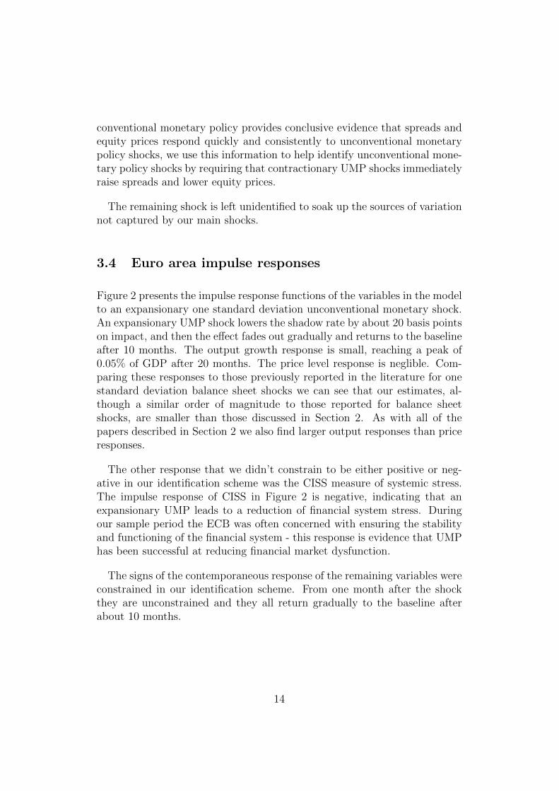
conventional monetary policy provides conclusive evidence that spreads andequity prices respond quickly and consistently to unconventional monetarypolicy shocks, we use this information to help identify unconventional mone-tary policy shocks by requiring that contractionary UMP shocks immediatelyraise spreads and lower equity prices.
The remaining shock is left unidentified to soak up the sources of variationnot captured by our main shocks.
3.4 Euro area impulse responses
Figure 2 presents the impulse response functions of the variables in the modelto an expansionary one standard deviation unconventional monetary shock.An expansionary UMP shock lowers the shadow rate by about 20 basis pointson impact, and then the effect fades out gradually and returns to the baselineafter 10 months. The output growth response is small, reaching a peak of0.05% of GDP after 20 months. The price level response is neglible. Com-paring these responses to those previously reported in the literature for onestandard deviation balance sheet shocks we can see that our estimates, al-though a similar order of magnitude to those reported for balance sheetshocks, are smaller than those discussed in Section 2. As with all of thepapers described in Section 2 we also find larger output responses than priceresponses.
The other response that we didn’t constrain to be either positive or neg-ative in our identification scheme was the CISS measure of systemic stress.The impulse response of CISS in Figure 2 is negative, indicating that anexpansionary UMP leads to a reduction of financial system stress. Duringour sample period the ECB was often concerned with ensuring the stabilityand functioning of the financial system - this response is evidence that UMPhas been successful at reducing financial market dysfunction.
The signs of the contemporaneous response of the remaining variables wereconstrained in our identification scheme. From one month after the shockthey are unconstrained and they all return gradually to the baseline afterabout 10 months.
14
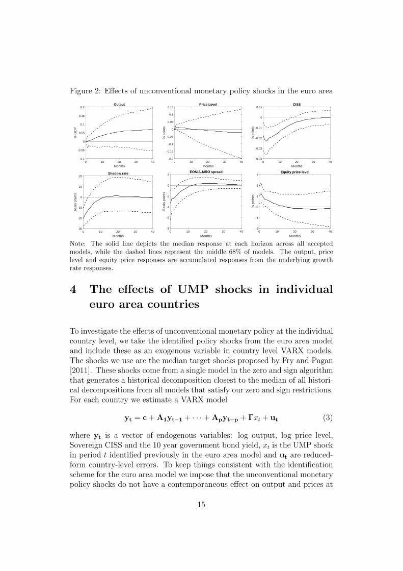
Figure 2: Effects of unconventional monetary policy shocks in the euro area
0 10 20 30 40
Months
-0.1
-0.05
0
0.05
0.1
0.15
0.2
% G
DP
Output
0 10 20 30 40
Months
-0.2
-0.15
-0.1
-0.05
0
0.05
0.1
0.15
% p
oint
s
Price Level
0 10 20 30 40
Months
-0.04
-0.03
-0.02
-0.01
0
0.01
% p
oint
s
CISS
0 10 20 30 40
Months
-30
-20
-10
0
10
20
basi
s po
ints
Shadow rate
0 10 20 30 40
Months
-8
-6
-4
-2
0
2
Bas
is p
oint
s
EONIA-MRO spread
0 10 20 30 40
Months
-2
-1
0
1
2
3
% p
oint
s
Equity price level
Note: The solid line depicts the median response at each horizon across all acceptedmodels, while the dashed lines represent the middle 68% of models. The output, pricelevel and equity price responses are accumulated responses from the underlying growthrate responses.
4 The effects of UMP shocks in individual
euro area countries
To investigate the effects of unconventional monetary policy at the individualcountry level, we take the identified policy shocks from the euro area modeland include these as an exogenous variable in country level VARX models.The shocks we use are the median target shocks proposed by Fry and Pagan[2011]. These shocks come from a single model in the zero and sign algorithmthat generates a historical decomposition closest to the median of all histori-cal decompositions from all models that satisfy our zero and sign restrictions.For each country we estimate a VARX model
yt = c + A1yt−1 + · · · + Apyt−p + Γxt + ut (3)
where yt is a vector of endogenous variables: log output, log price level,Sovereign CISS and the 10 year government bond yield, xt is the UMP shockin period t identified previously in the euro area model and ut are reduced-form country-level errors. To keep things consistent with the identificationscheme for the euro area model we impose that the unconventional monetarypolicy shocks do not have a contemporaneous effect on output and prices at
15
the country level either. That is, the first two elements of Γ are restrictedto zero. To impose these restrictions requires that we estimate the countrylevel VARX models with feasible generalised least squares, as described inLutkepohl [2005]11. As with the euro area model we include two lags of theendogenous variables.12
4.1 Data
For each country our monthly output series is a Chow-Lin interpolation ofquarterly GDP based on monthly industrial production and retail sales. Thiswas done using seasonally and calendar adjusted data on GDP, retail salesand industrial production from Eurostat. Data on the monthly price level(HICP) and on the 10-year government bond yield are also from Eurostat.As a measure of sovereign risk and dysfunction in sovereign bond markets ineach country, we make use of the Sovereign Composite Index of SystematicStress from the ECB’s Statistical Data Warehouse.
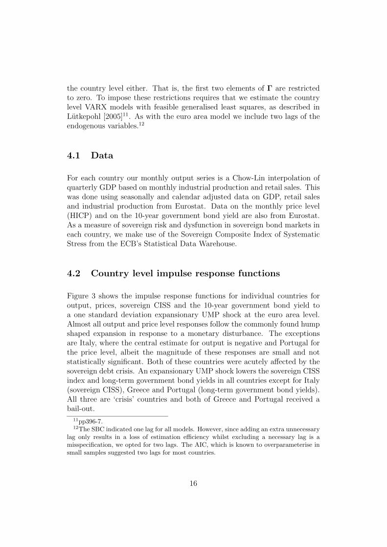
4.2 Country level impulse response functions
Figure 3 shows the impulse response functions for individual countries foroutput, prices, sovereign CISS and the 10-year government bond yield toa one standard deviation expansionary UMP shock at the euro area level.Almost all output and price level responses follow the commonly found humpshaped expansion in response to a monetary disturbance. The exceptionsare Italy, where the central estimate for output is negative and Portugal forthe price level, albeit the magnitude of these responses are small and notstatistically significant. Both of these countries were acutely affected by thesovereign debt crisis. An expansionary UMP shock lowers the sovereign CISSindex and long-term government bond yields in all countries except for Italy(sovereign CISS), Greece and Portugal (long-term government bond yields).All three are ‘crisis’ countries and both of Greece and Portugal received abail-out.
11pp396-7.12The SBC indicated one lag for all models. However, since adding an extra unnecessary
lag only results in a loss of estimation efficiency whilst excluding a necessary lag is amisspecification, we opted for two lags. The AIC, which is known to overparameterise insmall samples suggested two lags for most countries.
16

The responses also show economically significant differences between thecountries. The peak output responses in the Netherlands, Belgium and Spainare more than twice as large as in the crisis countries of Italy, Portugal andGreece. Likewise, Portugal and Greece have price level responses less thanone-fifth of the peak responses in Belgium and the Netherlands. Portugal andGreece also have economically significantly smaller responses for governmentbond yields, especially compared to Belgium.
Figure 3: Effects of unconventional monetary policy shocks in individualcountries
Output Prices Sovereign CISS 10yr yield
AUT
0 20 40 60
Months
-0.04
-0.02
0
0.02
0.04
0.06
% G
DP
0 20 40 60
Months
0
0.02
0.04
0.06
0.08
% p
oint
s
0 20 40 60
Months
-20
-15
-10
-5
0
5
Cha
nge
10-3
0 20 40 60
Months
-0.1
-0.08
-0.06
-0.04
-0.02
0
% p
oint
s
BEL
0 20 40 60
Months
-0.02
0
0.02
0.04
0.06
0.08
% G
DP
0 20 40 60
Months
-0.02
0
0.02
0.04
0.06
0.08
% p
oint
s
0 20 40 60
Months
-0.025
-0.02
-0.015
-0.01
-0.005
0
Cha
nge
0 20 40 60
Months
-0.12
-0.1
-0.08
-0.06
-0.04
-0.02
% p
oint
s
FIN
0 20 40 60
Months
-0.04
-0.02
0
0.02
0.04
0.06
% G
DP
0 20 40 60
Months
-0.02
0
0.02
0.04
% p
oint
s
0 20 40 60
Months
-10
-5
0
5
Cha
nge
10-3
0 20 40 60
Months
-0.06
-0.04
-0.02
0
0.02
0.04
% p
oint
s
FRA
0 20 40 60
Months
-0.02
0
0.02
0.04
0.06
% G
DP
0 20 40 60
Months
-0.04
-0.02
0
0.02
0.04
% p
oint
s
0 20 40 60
Months
-15
-10
-5
0
5
Cha
nge
10-3
0 20 40 60
Months
-0.1
-0.08
-0.06
-0.04
-0.02
0
% p
oint
s
DEU
0 20 40 60
Months
-0.04
-0.02
0
0.02
0.04
0.06
% G
DP
0 20 40 60
Months
-0.02
-0.01
0
0.01
0.02
0.03
% p
oint
s
0 20 40 60
Months
-10
-5
0
5
Cha
nge
10-3
0 20 40 60
Months
-0.06
-0.04
-0.02
0
0.02
% p
oint
s
Note: The dashed lines represent 90% bootstrapped confidence intervals calculated with
1000 replications under the assumption that the exogenous time series of UMP shocks is
fixed.
17
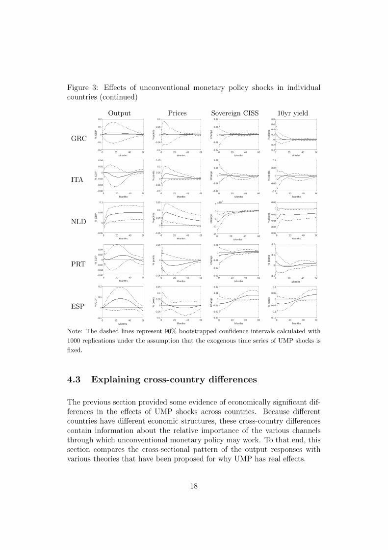
Figure 3: Effects of unconventional monetary policy shocks in individualcountries (continued)
Output Prices Sovereign CISS 10yr yield
GRC
0 20 40 60
Months
-0.2
-0.1
0
0.1
0.2
% G
DP
0 20 40 60
Months
-0.1
-0.05
0
0.05
0.1
% p
oint
s0 20 40 60
Months
-0.02
-0.01
0
0.01
0.02
Cha
nge
0 20 40 60
Months
-0.4
-0.2
0
0.2
0.4
0.6
0.8
% p
oint
s
ITA
0 20 40 60
Months
-0.06
-0.04
-0.02
0
0.02
0.04
% G
DP
0 20 40 60
Months
-0.1
-0.05
0
0.05
0.1
0.15
% p
oint
s
0 20 40 60
Months
-0.02
-0.01
0
0.01
0.02
Cha
nge
0 20 40 60
Months
-0.1
-0.05
0
0.05
0.1
% p
oint
s
NLD
0 20 40 60
Months
-0.05
0
0.05
0.1
% G
DP
0 20 40 60
Months
-0.05
0
0.05
0.1
0.15
% p
oint
s
0 20 40 60
Months
-15
-10
-5
0
5
Cha
nge
10-3
0 20 40 60
Months
-0.08
-0.06
-0.04
-0.02
0
0.02
% p
oint
sPRT
0 20 40 60
Months
-0.06
-0.04
-0.02
0
0.02
0.04
% G
DP
0 20 40 60
Months
-0.05
0
0.05
% p
oint
s
0 20 40 60
Months
-0.03
-0.02
-0.01
0
0.01
Cha
nge
0 20 40 60
Months
-0.1
0
0.1
0.2
% p
oint
s
ESP
0 20 40 60
Months
-0.1
0
0.1
0.2
% G
DP
0 20 40 60
Months
-0.1
-0.05
0
0.05
0.1
0.15
% p
oint
s
0 20 40 60
Months
-0.03
-0.02
-0.01
0
0.01
0.02
Cha
nge
0 20 40 60
Months
-0.15
-0.1
-0.05
0
0.05
0.1
% p
oint
s
Note: The dashed lines represent 90% bootstrapped confidence intervals calculated with
1000 replications under the assumption that the exogenous time series of UMP shocks is
fixed.
4.3 Explaining cross-country differences
The previous section provided some evidence of economically significant dif-ferences in the effects of UMP shocks across countries. Because differentcountries have different economic structures, these cross-country differencescontain information about the relative importance of the various channelsthrough which unconventional monetary policy may work. To that end, thissection compares the cross-sectional pattern of the output responses withvarious theories that have been proposed for why UMP has real effects.
18
4.3.1 The channels of unconventional monetary policy
In standard monetary models the stance of monetary policy can be fully de-scribed by the current and expected future short-term policy rate. Thesedetermine the present value of returns from holding assets so any policy thatreallocates assets between different agents in the economy has no effect onthe present value of returns and is therefore irrelevant (see Wallace [1981],Eggertsson and Woodford [2003] or Curdia and Woodford [2011]). For bal-ance sheet polices to have real effects requires there to be frictions in financialmarkets that are not included in standard monetary models. Haldane et al.[2016] lists six channels and their associated frictions which have been pro-posed in the literature for why balance sheet policies can have real effects.
The policy signalling channel works by signalling extra information aboutfuture short-term rates and relies on agents having imperfect informationabout how monetary policy will behave in future. By providing a crediblesignal about the future path of the nominal interest rate UMP can influenceconsumption and investment decisions today. In essence, this channel is avariant of forward guidance and relies on all of the standard channels workingin the future. If this is the most important channel countries who are mostlikely to benefit the most from future lower rates should have the biggesteffects.
However, it might be difficult to find evidence for the policy signallingchannel in a VAR framework because the signalling value of small deviationsaround the policy stance predicted by the policy rule is questionable. In thecase where the UMP shocks identified in the VAR framework are randomunexpected noise around the predictable part of monetary policy then agentsshouldn’t learn anything about the future path of nominal interest rates fromthe random disturbances.
The portfolio balance channel requires market participants to have a pre-ferred habitat or that there are limits to arbitrage. It is often argued thatbecause assets of different maturity are not perfect substitutes there are lim-its to arbitrage. If the portfolio balance channel is the dominant channelthen countries with more longer term debt should be the most affected byUMP.
The liquidity premium channel requires markets to be dysfunctional withabnormally high liquidity premia. Because the central bank can improveliquidity and reduce liquidity premia, UMP can restore normality to financial
19
markets and increase credit intermediation. As such, if the liquidity premiumchannel is the dominant transmission channel we should expect countrieswhere UMP reduces market stress measures the most to also have the largestoutput effects.
The exchange rate channel works the same way as with conventional mon-etary policy. That is, expansionary UMP causes an exchange rate deprecia-tion which boosts exports and reduces imports. If the exchange rate channelis the dominant channel then countries that trade the most with non-eurocountries should respond the most.
The confidence/uncertainty channel works through UMP reducing marketvolatility or by convincing market participants that future economic per-formance will be better. As such, UMP reduces the risk of bad economicoutcomes and should have larger effects in countries where the risk of badeconomic outcomes is reduced the most.
The final channel listed by Haldane et al. [2016], the bank lending channel,relies on some economic agents having no substitutes for bank loans, hencewhen UMP increases the price of assets on banks’ balance sheets the extraloans these banks can make add to the aggregate quantity of loans. Bankswith weak balance sheets are the most constrained by the value of their assets.Hence weak banks’ lending behaviour is most dependent on the changes in thevalue of the assets they hold caused by UMP shocks. Moreover, it is typicallysmall firms and households who are most likely to have no alternatives tobank loans. Hence, we should expect larger effects of UMP in countries withweaker banks and more small firms.
As Wieladek and Garcia Pascual [2016] reported, when an economy is closeto potential economic stimulus is more likely to end up as increased inflationrather than extra output. As such we should also expect UMP to have largeroutput effects in countries with bigger output gaps.
4.3.2 Cross-country correlations
To get an idea which channels are the most important Figure 4 shows somecross-correlations between the magnitude of the country level responses andindicator variables that proxy the expected strength of the various channels.Cross-correlations are, of course, only suited to identifying the dominantchannels, since any weaker channels will not be visible due to the effects of
20

the stronger channels.13 We show cross-correlations here because 10 cross-country observations are too few for regression analysis.
As described above, if the policy signalling channel is the dominant mech-anism through which UMP affects the macroeconomy, then we would expectthe largest output effects in those countries most affected by normal mone-tary policy shocks. Georgiadis [2015] reports that changes in interest rateshave larger effects in countries where the output share of sectors that are in-terest sensitive is greater. Specifically, Georgiadis [2015] found that euro areacountries with larger shares of manufacturing and construction have largeroutput effects from conventional monetary policy shocks, although the re-lationship was not statistically significant for construction. The first twocorrelations in Figure 4 compares the peak output responses to UMP shockswith the manufacturing and construction shares. We find no relationship be-tween the peak output effect and the manufacturing share. The correlationbetween the peak output effect and the construction share is positive butit is not quite statistically significant at conventional levels of significance.Moreover, the positive relationship is highly dependent on just one observa-tion: the peak response in Spain, which is an outlier in our estimates. Allin all, our results argue against the policy signalling channel being the maintransmission channel.
The next correlation looks at whether there is a relationship between theaverage remaining maturity of outstanding government debt and the peakoutput effect. We find no evidence of a relationship, which is suggestive thatthe portfolio balance channel is not the dominant channel. We do, however,find countries that had larger peak output effects also had larger responses ofthe ten year government bond yield in our country VARX models, althoughit isn’t quite statistically significant. As Wieladek and Garcia Pascual [2016]note, significant movements in long-term bond yields is a prerequisite for theportfolio balance channel. Even so, we would expect the portfolio balancechannel to show up in countries where the relative proportion of outstandinglong-term debt changes the most.
13Even for the dominant channels the noise generated by the weaker channels will, onaverage, lower the statistical significance of the correlations. However, we also performmultiple cross-correlations which, of course, raises the probably of finding correlationswith apparently significant correlations. It’s not clear how to balance these two factors toproduce a measure of the true statistical significance, so we report standard p-values. Inany case, the purpose of this section is to highlight channels that are very unlikely to bethe dominant transmission channel.
21

Figure 4: Cross-correlations of peak output effect
AUT
BEL
FIN
FRA
GRC
ITA
NLD
PRT
ESP
0
0.02
0.04
0.06
0.08
0.1
8 10 12 14 16 18 20
%
Manufacturing as % GDP (average 2009-2016)
Correlation = -0.23p-value = 0.30R2 = 0.05
AUT
BEL
FIN
FRA
DEUGRC
ITA
NLD
PRT
ESP
0
0.02
0.04
0.06
0.08
0.1
3 4 5 6 7 8
%
Construction as %GDP (average 2009-2016)
Correlation = 0.44p-value = 0.15R2 = 0.19
BEL
FIN
FRA
DEUGRC
ITA
NLD
PRT
ESP
0.00
0.02
0.04
0.06
0.08
0.10
3 5 7 9
%
Average remaining debt maturity in 2008
Correlation = -0.10p-value = 0.37R2 = 0.01
AUT
BEL
FIN
FRA
DEUGRC
ITA
NLD
PRT
ESP
0
0.02
0.04
0.06
0.08
0.1
-0.1 -0.08 -0.06 -0.04 -0.02 0
%
Peak response of 10yr bond yield
Correlation = -0.46p-value = 0.13R2 = 0.21
AUT
BEL
FIN
FRA
DEUGRC
ITA
NLD
PRT
ESP
0
0.02
0.04
0.06
0.08
0.1
-0.02 -0.015 -0.01 -0.005 0
%
Peak response of sovereign CISS
Correlation = -0.58p-value = 0.06R2 = 0.34
AUT
BEL
FIN
FRA
DEUGRC
ITA
NLD
PRT
ESP
0
0.02
0.04
0.06
0.08
0.1
0 20 40 60 80
%
Non euro goods trade in 2008 as % GDP
Correlation = 0.22p-value = 0.15R2 = 0.05
In so far as dysfunction raises the risk premia on sovereign bonds, thechange in the ten year government bond yield also measures how much aUMP shock reduces market dysfunction. Another more direct measure ofmarket dysfunction is the peak effect on the sovereign CISS indicator in ourcountry VARX models. For both of these indicators we find that countries
22

Figure 4: Cross-correlations of peak output effect (continued)
AUT
BEL
FIN
FRA
DEUGRC
ITA
NLD
PRT
ESP
0
0.02
0.04
0.06
0.08
0.1
0 0.5 1 1.5
%
Bank health in 2010
Correlation = 0.56p-value = 0.07R2 = 0.27
AUT
BEL
FIN
FRA
DEUGRC
ITA
NLD
ESP
0
0.02
0.04
0.06
0.08
0.1
0.2 0.25 0.3 0.35 0.4 0.45 0.5
%
Share of small firms in % value added
Correlation = 0.23p-value = 0.31R2 = 0.05
AUT
BEL
FIN
FRA
DEUGRC
ITA
NLD
PRT
ESP
0
0.02
0.04
0.06
0.08
0.1
45 65 85 105 125
%
Government debt as % GDP in 2010
Correlation = -0.47p-value = 0.12R2 = 0.22
AUT
BEL
FIN
FRA
DEUGRC
ITA
NLD
PRT
ESP
0
0.02
0.04
0.06
0.08
0.1
0 2 4 6 8
%
Average output gap (2009-14)
Correlation = 0.12p-value = 0.36R2 = 0.02
AUTFIN
FRA
DEUGRC
ITA
NLD
PRT
ESP
0
0.02
0.04
0.06
0.08
0.1
0 20 40 60 80 100 120
%
Average share of variable rate loans 2008-2016
Correlation = -0.25p-value = 0.30R2 = 0.06
AUT
BEL
FIN
FRA
DEUGRC
ITA
NLD
PRT
ESP
0
0.02
0.04
0.06
0.08
0.1
0 20 40 60 80 100 120
%
Average share of variable rate mortgages 2008-2016
Correlation = -0.27p-value = 0.29R2 = 0.07
that had larger reductions in market dysfunction had larger peak outputresponses. The relationship with the peak effect on sovereign CISS is sta-tistically significant at the 10% level and for the ten year bond yield it isborderline statistically significant. Furthermore, neither of the correlations
23

is driven by the large output response observed for Spain, since their sovereignCISS and ten year bond yield responses are close to the average. These cor-relations could point towards either the liquidity premium channel or theconfidence/uncertainty channel being an important transmission channel.
To evaluate the importance of the exchange rate channel we have createdan openness variable that is the sum of goods exports and imports to non-euro countries14. As expected, we find that countries that trade more withnon-euro countries have experienced larger output effects from UMP shocks,although the relationship only has a p-value of 0.15. However, the Spanishdata point is working strongly against finding a positive relationship. Themost obvious evidence against the exchange rate channel would appear to bethe small response of euro area inflation that we and others have reportedfollowing UMP shocks, as one would expect exchange rate changes to passthrough into domestic prices. However, Comunale and Kunovac [2017] pro-vide evidence that the pass through of exchange rate movements to HICPinflation in the euro area is limited, which means our inflation responsescannot rule out the exchange rate channel.
We also find statistically significant correlations between the peak outputresponses from our country level models and a number of indicators associ-ated with bank health. The bank health variable in Figure 4 is the averageof non-performing loans, return on equity and return on assets in 201015. Wefind a significantly positive relationship with our bank health indicator anda negative correlation with government debt, which is of borderline statis-tical significance. The latter may also be indicative of bank health becauseof the link between the health of government finances in the euro area arehighly intertwined with the health of the banks who hold their debt. Thisrelationship between bank health and the effectiveness of UMP mirrors thatreported earlier by the studies described in Section 2. However, compared tothe predictions made by the bank lending channel, these relationships havethe wrong sign: countries with healthier banks have larger responses to UMPshocks. Can we explain this anomaly? Firstly, we can speculate that thesepolicies may depend non-linearly on economic circumstances. One issue with
14This includes Bulgaria and Denmark as euro countries since their exchange rates aretied closely to the euro. We include only trade in goods as the trade in services data fromUN Comtrade wasn’t complete for all of the countries in our sample.
15We chose 2010 because it is close to the start of our sample period and thereforeunlikely to have been overly influenced by the UMP we are studying. We chose 2010 over2009 because the latter year was the main year of the Great Recession and some indicatorsfor 2009 are not indicative of more normal times.
24

European banks is the link between weak banks and weak sovereigns where European banks’ asset holdings are strongly biased in favour of the debt of their own sovereigns. If market participants perceive that a bank’s solvability depends on their sovereign receiving a bailout and a small change in market rates still leaves their sovereign in need of a bailout, then the small change in market conditions that follow a UMP shock will still leave that bank con-strained. Hence countries with large outstanding government debts should not react in the same way to the bank lending channel. Another possibil-ity is that recent regulatory changes and market participant’s perceptions of the riskiness of banks in general has forced banks to build up their cap-ital. In countries with healthy banks already at or close to the new capital standards the increased value of assets on their balance sheets can be used to finance new lending. For countries with weak banks the effects of UMP shocks will increase the value of the assets on their balance sheets but these gains will more likely be used to build up sufficient capital to satisfy market participants or new regulations. Obviously our sample period of UMP also includes the TLTRO programme where changes in the central bank’s balance sheet were conditional on the receiving banks making new loans. However, it is unclear how fungible the TLTRO loans were with other loans on banks’ balance sheets in practice.
We also find a statistically insignificant positive relationship between the importance of small firms in an economy and the peak output effects, which is the sign predicted by the bank lending channel. Additionally, we find no evidence of a relationship between the size of output gaps and the effective-ness of UMP shocks. Finally, in contrast to Wieladek and Garcia Pascual [2016] we find no relationship between the share of variable rate loans (either all loans or just mortgage loans) and the peak output effects.
5 Conclusion
In this paper we have estimated the effects of unconventional monetary policy shocks in the euro area in an SVAR framework using zero and sign restric-tions for identification. We have found weak evidence that expansionary un-conventional monetary policy shocks increase output growth, but the effects on inflation at the aggregate euro area level are economically insignificant. We have taken the identified monetary policy shocks and employed these in country level models to gain more insight into the transmission of uncon-ventional monetary policy. We have found a range of responses across the
25

countries in our sample, and those differences in the magnitudes of outputresponses are most consistent with the liquidity premium channel, the con-fidence/uncertainty channel and the exchange rate channel. We also foundthat larger peak output responses are associated with healthier banking sys-tems at the start of our sample and lower government debts.
These results are naturally subject to a considerable degree of uncertainty.The sample period is short, which make precise estimation difficult, and cor-relation is not causation. Nonetheless, our empirical evidence is consistentwith some of the main theories for the transmission of unconventional mon-etary policy.
26
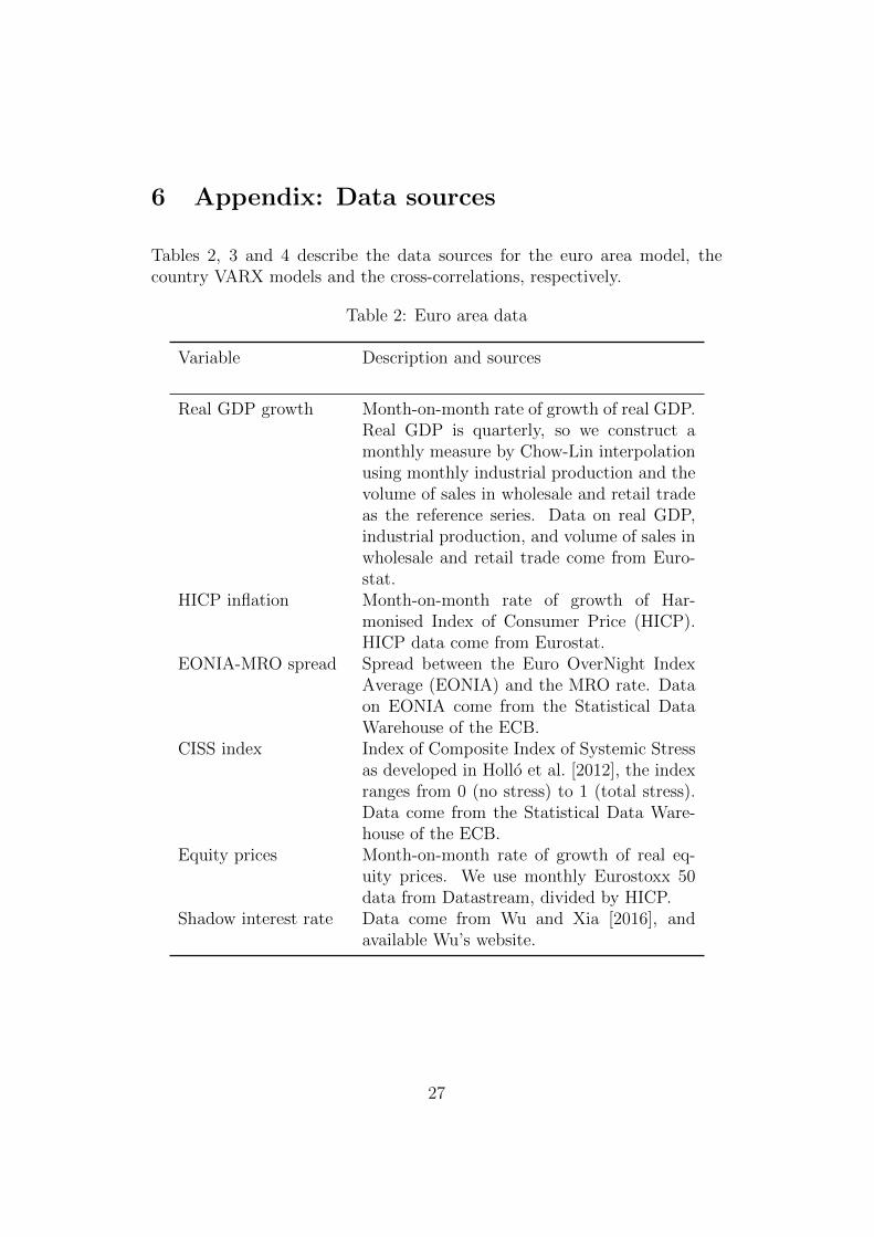
6 Appendix: Data sources
Tables 2, 3 and 4 describe the data sources for the euro area model, thecountry VARX models and the cross-correlations, respectively.
Table 2: Euro area data
Variable Description and sources
Real GDP growth Month-on-month rate of growth of real GDP.Real GDP is quarterly, so we construct amonthly measure by Chow-Lin interpolationusing monthly industrial production and thevolume of sales in wholesale and retail tradeas the reference series. Data on real GDP,industrial production, and volume of sales inwholesale and retail trade come from Euro-stat.
HICP inflation Month-on-month rate of growth of Har-monised Index of Consumer Price (HICP).HICP data come from Eurostat.
EONIA-MRO spread Spread between the Euro OverNight IndexAverage (EONIA) and the MRO rate. Dataon EONIA come from the Statistical DataWarehouse of the ECB.
CISS index Index of Composite Index of Systemic Stressas developed in Hollo et al. [2012], the indexranges from 0 (no stress) to 1 (total stress).Data come from the Statistical Data Ware-house of the ECB.
Equity prices Month-on-month rate of growth of real eq-uity prices. We use monthly Eurostoxx 50data from Datastream, divided by HICP.
Shadow interest rate Data come from Wu and Xia [2016], andavailable Wu’s website.
27

Table 3: VARX data
Variable Description and sources
Real GDP Monthly real GDP. Real GDP are at quar-terly frequency, and we construct monthlymeasures using a Chow-Lin interpolationprocedure where monthly industrial produc-tion and the volume of retail sales. Data onreal GDP, industrial production, and volumeof retail sales come from Eurostat.
HICP Monthly Harmonised Index of ConsumerPrice (HICP) from Eurostat.
Sovereign CISS index Sovereign debt market component of theComposite Index of Systemic Stress as de-veloped in Hollo et al. [2012], from the Sta-tistical Data Warehouse of the ECB.
Ten year governmentbond yield
From Eurostat.
28

Table 4: Data for cross-country correlations
Variable Description Data Source
Manufacturingshare
Share of manufacturing in to-tal value added (2009-2016)
World Bank
Constructionshare
Share of construction in to-tal value added (2009-2016)
OECD
Remainingdebt maturity
Average remaining maturityof government debt (2008)
ECB (BISfor Germany)
Goods tradeopenness
Goods exports plus importsto non-euro countries as a %of GDP (average 2009-2016)
UN Comtrade
Bank healthBank health (average of non-performing loans, return onequity and return on assets)
ECB
Small firmsOne minus share of firms larger
than 250 employees in valueadded (average 2010-2015)
Eurostat
Governmentdebt
Central government debt aspercentage of GDP (2010)
World Bank
Output gap Average output gap (2009-2014) OECD
Share ofvariable loans
Share of all new loans to householdsand non-financial corporationswith fixed interest period up to12 months (average 2008-2016)
ECB
Share ofvariable
mortgages
Share of all new mortgage loans tohouseholds with fixed interest periodup to 12 months (average 2008-2016)
ECB
29

References
Philippe Andrade, Johannes Breckenfelder, Fiorella De Fiore, Peter Karadi,and Oreste Tristani. The ECB’s asset purchase programme: an early as-sessment. Working Paper Series 1956, European Central Bank, September2016.
Jonas E. Arias, Juan F. Rubio-Ramırez, and Daniel F. Waggoner. InferenceBased on SVARs Identified with Sign and Zero Restrictions: Theory andApplications. Dynare Working Papers 30, CEPREMAP, January 2014.
Christiane Baumeister and Luca Benati. Unconventional Monetary Policyand the Great Recession: Estimating the Macroeconomic Effects of aSpread Compression at the Zero Lower Bound. International Journal ofCentral Banking, 9(2):165–212, June 2013.
John Beirne, Lars Dalitz, Jacob Ejsing, Magdalena Grothe, Simone Man-ganelli, Fernando Monar, Benjamin Sahel, Matjaz Susec, Jens Tapking,and Tana Vong. The impact of the Eurosystem’s covered bond purchaseprogramme on the primary and secondary markets. Occasional Paper Se-ries 122, European Central Bank, January 2011.
Fischer Black. Interest rates as options. The Journal of Finance, 50(5):1371–1376, 1995.
Jef Boeckx, Maarten Dossche, and Gert Peersman. Effectiveness and Trans-mission of the ECB’s Balance Sheet Policies. International Journal ofCentral Banking, 13(1):297–333, February 2017.
Claudio Borio and Anna Zabai. Unconventional monetary policies: a re-appraisal. BIS Working Papers 570, Bank for International Settlements,July 2016.
Pablo Burriel and Alessandro Galesi. Uncovering the heterogeneous effects ofECB unconventional monetary policies across euro area countries. Work-ing Papers 1631, Banco de Espana;Working Papers Homepage, December2016.
Lawrence J Christiano, Martin Eichenbaum, and Charles L Evans. Nominalrigidities and the dynamic effects of a shock to monetary policy. Journalof political Economy, 113(1):1–45, 2005.
Mariarosaria Comunale and Davor Kunovac. Exchange rate pass-throughin the euro area. Working Paper Series 2003, European Central Bank,January 2017.
30

Vasco Curdia and Michael Woodford. The central-bank balance sheet asan instrument of monetarypolicy. Journal of Monetary Economics, 58(1):54–79, January 2011.
Milan Damjanovic and Igor Masten. Shadow short rate and monetary policyin the euro area. Empirica, 43(2):279–298, 2016.
Gauti B. Eggertsson and Michael Woodford. The Zero Bound on InterestRates and Optimal Monetary Policy. Brookings Papers on Economic Ac-tivity, 34(1):139–235, 2003.
Adam Elbourne and Jakob de Haan. Financial structure and monetary policytransmission in transition countries. Journal of Comparative Economics,34(1):1–23, 2006.
Renee Fry and Adrian Pagan. Sign Restrictions in Structural Vector Au-toregressions: A Critical Review. Journal of Economic Literature, 49(4):938–960, December 2011.
Leonardo Gambacorta, Boris Hofmann, and Gert Peersman. The Effective-ness of Unconventional Monetary Policy at the Zero Lower Bound: ACross-Country Analysis. Journal of Money, Credit and Banking, 46(4):615–642, 06 2014.
Luca Gambetti and Alberto Musso. The macroeconomic impact of the ECB’sexpanded asset purchase programme (APP). Working Paper Series 2075,European Central Bank, June 2017.
Georgios Georgiadis. Examining asymmetries in the transmission of mone-tary policy in the euro area: Evidence from a mixed cross-section globalVAR model. European Economic Review, 75(C):195–215, 2015.
Reinder Haitsma, Deren Unalmis, and Jakob de Haan. The impact of theECB’s conventional and unconventional monetary policies on stock mar-kets. Journal of Macroeconomics, 48(C):101–116, 2016.
Andrew Haldane, Matt Roberts-Sklar, Tomasz Wieladek, and Chris Young.QE: The Story so far. Bank of England working papers 624, Bank ofEngland, October 2016.
James Douglas Hamilton. Time series analysis, volume 2. Princeton univer-sity press Princeton, 1994.
31
Lars Peter Hansen and Thomas J. Sargent. Two difficulties in interpretingvector autoregressions. In Lars Peter Hansen and Thomas J. Sargent, ed-itors, Rational Expectations Econometrics, pages 77–119. Westview Press,Boulder, CO., 1991.
Daniel Hollo, Manfred Kremer, and Marco Lo Duca. CISS - a compositeindicator of systemic stress in the financial system. Working Paper Series1426, European Central Bank, March 2012.
Soyoung Kim and Nouriel Roubini. Exchange rate anomalies in the indus-trial countries: A solution with a structural VAR approach. Journal ofMonetary Economics, 45(3):561–586, June 2000.
Manfred Kremer. Macroeconomic effects of financial stress and the role ofmonetary policy: a VAR analysis for the euro area. International Eco-nomics and Economic Policy, 13(1):105–138, January 2016.
Leo Krippner. A comment on Wu and Xia (2015), and the case for two-factor Shadow Short Rates. CAMA Working Papers 2015-48, Centre forApplied Macroeconomic Analysis, Crawford School of Public Policy, TheAustralian National University, December 2015a.
Leo Krippner. Zero Lower Bound Term Structure Modeling: A Practitioner’sGuide. Palgrave Macmillan, 2015b.
Eric M. Leeper, Todd B. Walker, and Shu-Chun Susan Yang. Fiscal Foresightand Information Flows. Econometrica, 81(3):1115–1145, 05 2013.
Wolfgang Lemke and Andreea Liliana Vladu. Below the zero lower bound: ashadow-rate term structure model for the euro area. Working Paper Series1991, European Central Bank, January 2017.
Helmut Lutkepohl. New introduction to multiple time series analysis.Springer Science & Business Media, 2005.
Helmut Lutkepohl and Markus Kratzig. Applied time series econometrics.Cambridge university press, 2004.
Frederic S. Mishkin. The Channels of Monetary Transmission: Lessons forMonetary Policy. NBER Working Papers 5464, National Bureau of Eco-nomic Research, Inc, February 1996.
Matthias Paustian. Assessing sign restrictions. The BE Journal of Macroe-conomics, 7(1), 2007.
32

Gert Peersman. What caused the early millennium slowdown? evidencebased on vector autoregressions. Journal of Applied Econometrics, 20(2):185–207, 2005.
Gert Peersman and Roland Straub. Technology shocks and robust sign re-strictions in a euro area svar. International Economic Review, 50(3):727–750, 2009.
Harald Uhlig. What are the effects of monetary policy on output? resultsfrom an agnostic identification procedure. Journal of Monetary Economics,52(2):381–419, 2005.
Neil Wallace. A Modigliani-Miller Theorem for Open-Market Operations.American Economic Review, 71(3):267–274, June 1981.
Tomasz Wieladek and Antonio Garcia Pascual. The European Central Bank’sQE: A new hope. CEPR Discussion Papers 11309, C.E.P.R. DiscussionPapers, June 2016.
Jing Cynthia Wu and Fan Dora Xia. Measuring the Macroeconomic Impactof Monetary Policy at the Zero Lower Bound. Journal of Money, Creditand Banking, 48(2-3):253–291, 03 2016.
33

Publisher:
CPB Netherlands Bureau for Economic Policy Analysis P.O. Box 80510 | 2508 GM The HagueT (088) 984 60 00
February 2018