Urban Studies, Vol. 41, No. 7, 1333–1348, June 2004

The Effects of Portland’s Urban Growth Boundaryon Urban Development Patterns and Commuting

Myung-Jin Jun

[Paper first received, February 2003; in final form, October 2003]

Summary. This research investigates the effects of Portland’s urban growth boundary (UGB)on urban development patterns and mobility. Three different methods are adopted for evaluatingPortland’s UGB: intermetropolitan comparisons; comparisons inside and outside the UGB; and,statistical analyses utilising regression models. Intermetropolitan comparisons do not support theconclusion that Portland’s UGB has been effective in slowing down suburbanisation, enhancinginfill development and reducing auto use. A significant level of spillover from the counties inOregon to Clark County of Washington took place during the 1990s, indicating that the UGBdiverted population growth into Clark County. Results from the statistical analyses also supportthe above findings. The UGB dummy variable was not significant during the 1980s and 1990s,indicating that the UGB had little impact on the location of new housing construction during the1980s and 1990s. Unlike the UGB, the Clark County dummy variable is significant for bothmodels, supporting the spillover effects of the UGB.

1. Introduction

Since the first US urban growth boundary(UGB) was established in Lexington, Ken-tucky, in 1958 (Nelson and Duncan, 1995),UGBs have become one of the most popularurban growth management tools. By 1999,more than 100 cities and counties in the UShad adopted UGBs and three states, Oregon,Tennessee and Washington, had passed state-wide mandates for UGBs (Staley et al.,1999). Oregon adopted growth managementlegislation in 1973 and Portland’s UGB wasproposed in 1977 and approved by the statein 1980. The Washington Growth Manage-ment Act was passed in 1990 and ClarkCounty, WA, introduced a UGB in 1995(Bae, 2001).

Perhaps no other city in the US has beenmentioned as often as Portland in urban plan-

ning literature. Portland’s UGB has been inthe centre of controversy for the past twodecades between the pro-marketeers andgovernment intervention advocates. As anadvocate of UGBs, the American PlanningAssociation recommends that UGBs be es-tablished

to promote compact and contiguous devel-opment patterns that can be efficientlyserved by public services and to preserveor protect open space, agricultural land,and environmentally sensitive areas (Dinget al., 1999, p. 53).

On the other hand, Jan Brueckner argues that

urban growth boundaries can easily yieldundesirably draconian outcomes, becausethey are not directly linked to the underly-

Myung-Jin Jun is in the Department of Urban and Regional Planning, Chung-Ang University, Ansungsi, Kyunggido, South Korea.Fax: 82 31 675 1381. E-mail: mjjun1@post.cau.ac.kr. The work was supported by the Korea Research Foundation Grant(KRF-2001-013-C00120).

0042-0980 Print/1360-063X On-line/04/071333–16 2004 The Editors of Urban StudiesDOI: 10.1080/0042098042000214824

MYUNG-JIN JUN1334

ing market failures responsible for sprawl(Brueckner, 2000, p. 170).

In spite of numerous UGB studies, there isno agreement about their effectiveness.Given these differing views, this paper willattempt to evaluate the effects of Portland’sUGB on urban development patterns, trans-port choices and mobility. Specifically, theassessment will focus on whether Portland’sUGB: controls sprawl and encourages infilldevelopment; curtails automobile usage andpromotes public transit ridership; and, main-tains mobility.

There is the persisting problem of how toseparate the effects of Portland’s UGB fromautonomous market forces and other land useand growth management policies. Althoughit is difficult to assess to what extent Port-land’s UGB has contributed to current urbanspatial formation and mobility, it is feasibleto evaluate if Portland’s UGB has had anyinfluence on urban development patterns.This can be assessed in the following ways:by comparing Portland with other metropoli-tan regions; by comparing inside and outsidethe UGB within Portland; and, by statisticalanalyses.

The remainder of this paper contains sixsections. Sections 2 and 3 introduce Port-land’s UGB and review the previous re-search. Section 4 compares Portland withother metropolitan regions in the US. In sec-tion 5, comparisons are made inside andoutside the UGB within Portland. Section 6introduces the standard least square esti-mation method to assess if the UGB affectedurban spatial formation. Section 7 containsconclusions and suggested policy implica-tions.

2. Portland’s Urban Growth Boundary

Metro, the managing body of Portland’sUGB, defines the UGB as

a legal boundary separating urbanizableland from rural land … The boundary con-trols urban expansion onto farm, forest,and resource lands. At the same time, land,roads, utilities, and other urban services

are more efficiently distributed within theurban boundary (Metro, 2002, p. 1).

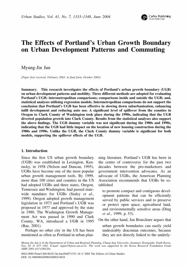
Under Oregon law, Metro has the responsi-bility for maintaining a 20-year supply ofresidential land to accommodate urban ac-tivity and growth for the Portland metropoli-tan area. The Portland UGB covers 24 cities(including the urban portions of Washington,Multnomah and Clackamas counties) thatcontained 369 square miles with 1.3 millionresidents in 2000 (see Figure 1).

Three co-ordinated measures are generallyused in managing the UGB: phased develop-ment inside the UGB; limiting developmentoutside the UGB; and, flexible boundary ofthe UGB (Daniels, 1999). Phased develop-ment is a way to encourage contiguous de-velopment inside the boundary by buildingonly on open land that is adjacent to existingdevelopment. Local governments in Oregonare required to make public facility plans thatensure that zones inside the UGB will bedeveloped at urban densities. The localgovernment provides an incentive to devel-opers in the permit process by quickly re-sponding (within four months) to adeveloper’s proposed project if the project isgoing inside the UGB.

Along with phased development inside theUGB, counties in Oregon are given the auth-ority of zoning rural lands for exclusive farmuse and forest conservation outside the UGB.As of 1998, about 25 million acres of farmand forest have been zoned for exclusivefarm use and timber conservation (Daniels,1999). In addition, Oregon designated ruralresidential zones with 3–5 acre minimum lotsizes outside the UGB. The boundaries of theUGB are designed to change over time. Theboundary of Portland’s UGB has changedabout three dozen times as the metropolitanpopulation has increased by 700 000 peoplesince 1979.

3. Literature Review

There are numerous studies on the effects ofUGBs on urban development patterns andhousing markets. Since the effects of UGBs

PORTLAND’S URBAN GROWTH BOUNDARY 1335

Figure 1. Portland’s urban growth boundary.

on land and housing prices are well docu-mented (Knaap, 2000) and beyond the scopeof this paper, this review focuses on theeffect of UGBs on urban development pat-terns.

Empirical analyses show contradicting re-sults about the effects of UGBs on urbandevelopment patterns. Some argue that Port-land’s UGB has contributed to controllingurban sprawl and urbanised density increases(Patterson, 1999; Nelson and Moore, 1993;Kline and Alig, 1999), while others insistthat Portland’s trend of suburbanisation andland use patterns is no better than those ofother metropolitan areas (Richardson andGordon, 2001; Cox, 2001).

Nelson and Moore (1993) analyse residen-tial building permits, residential land divi-sions and density of residential developmentinside and outside Portland’s UGB between1985 and 1989. They conclude that mostregional development has been directed

within the UGB. However, they argue thatconsiderable development continues outsidethe UGB and that “efficient expansion of theUGB in the future may be jeopardised bylow-density development patterns along theboundary” (Nelson and Moore, 1993,p. 302).

One Thousand Friends of Oregon (1991)conduct similar studies in analysing thedensity of residential development in Port-land from 1985 to 1989. They find thatactual development densities in multiple-family zones are closer to the planned den-sity, reaching about 90 per cent, whereasthose in single-family zones fall short of theplanned density level, approaching only 66per cent.

Kline and Alig (1999) analyse farm andforestland conversion in Oregon and Wash-ington and find that most urban developmentis concentrated inside the UGB. However,they are unable to provide evidence that the

MYUNG-JIN JUN1336

UGB protected farm and forestland outsidethe UGB from urban development.

Although these studies conclude that theUGB makes significant contributions to con-tain urban development inside the UGB, theirfindings cannot be generalised because ofseveral limitations in their research. Theyexamine building permits and densitychanges for the three counties on which theUGB is drawn, ignoring Clark County, WA,where growth from the three counties mayspill over. Knaap (2000) also argues that ifPortland is defined by the UGB, then it hasgrown by only 1.2 per cent in the past 20years. However, if all urban footprints areincluded, then Portland has grown by about29 per cent. Another limitation of the abovestudies is the time-span of their research.Two of the studies draw conclusions fromdata analysis covering the 5 years between1985 and 1989. Since urban land uses changeover a relatively long period of time, a 5-yeartrend analysis does not represent a long-termtrend of urban development.

Richardson and Gordon (2001) comparePortland with Los Angeles and find that sub-urbanisation and decentralisation in both re-gions are quite similar. They also examinehousing affordability and transit ridership inboth regions and conclude that growth man-agement controls have almost no impact.

Bae (2001) analyses cross-border impactsof the UGB between Portland and ClarkCounty, WA. She examines population andemployment growth, jobs–housing imbal-ances and traffic flows for the four countiesin the Portland metropolitan region. She con-cludes that the growth management policiesdo not stop growth; rather, they merely divertgrowth into other locations—especially,Clark County, Washington, which has thefastest population growth in the state ofWashington.

Cox (2001) compares Portland with At-lanta by analysing 17 variables includingpopulation and employment growth, auto useand transit ridership. He concludes that

Despite its smart growth policies, Portlandis not different from other urban areas.

Most growth is in peripheral areas, withcomparatively little growth in the center(Cox, 2001, p. 21).

Studies arguing that the UGB has little im-pact on urban development patterns havelimitations because of the generalisation intheir findings. Even though these studies userecent data, they do not select enough sam-ples to conduct intermetropolitan compari-sons. Findings from a comparative analysisof a couple of metropolitan regions do notrepresent the relative performance of Port-land’s UGB among other metropolitan re-gions.

This paper is distinguished from earlierworks in several respects. This research em-ploys more dependable methods than otherstudies to assess the effects of Portland’sUGB. Unlike Richardson and Gordon (2001)and Cox (2001) who compared Portland withone or two other metropolitan regions, thispaper compares Portland with all othermetropolitan regions in the US, controllingfor population size. As a result, a more ob-jective evaluation of the effects of the UGBis possible. Furthermore, this paper intro-duces standard regression models in order toestimate the effects of the UGB on urbandevelopment patterns. Data reliability is an-other advantage of this paper. The recentrelease of the 2000 census STF3 makes itpossible to analyse 20-year trends on variousissues from 1980 to 2000, which is asufficient time-period for measuring the ef-fects of the UGB.

4. How Is Portland Different from OtherMetropolitan Regions?

This section compares the Portland PMSA(Primary Metropolitan Statistical Area) withother metropolitan areas for the followingvariables: urbanised population, urbanisedland area, population density in urbanisedarea, employment in central city, housingunit proportions in the urbanised area, autoand transit users, and mean commuting time.Thirty-two metropolitan regions in the USwith populations over one million in 1980were selected for comparison.

PORTLAND’S URBAN GROWTH BOUNDARY 1337

Table 1. Population, land area, and density in the Portland urbanised area, 1980–2000

RankPercentage change19901980 (out of 32)2000 1980–2000

Urbanised population (000s) 81026 54.31172 1583Land (square miles) 349 388 474 935.8Density 2940.3 3021.0 3340.0 1513.6

Source: US Bureau of Census, STF3, 1980, 1990 and 2000.

Table 2. Growth rate and rank for the selected variable in Portland

Growth rate, 1980–2000 Rank(out of 32)Variables (percentage)

Employment in central city 70.8 6Housing units in urbanised area 54.4 16

12Auto users 69.9Public transit users 1126.1Mean commuting time 1514.5

Source: US Bureau of Census, STF3, 1980 and 2000.

Table 1 presents changes in Portland’spopulation, land size and density in the ur-banised area over the past two decades. Ur-banised population and land are goodindicators of urbanisation trends. The ur-banised population has increased by 54 percent, while the urbanised land area increasedby 36 per cent over the 1980–2000 period.Portland’s growth rates are ranked 8th forurbanised population and 9th for urbanisedland among 32 metropolitan areas. Thesefindings imply that urbanised land area andpopulation have increased at a faster ratethan other metropolitan areas, making Port-land one of top 10 fastest-growing metropoli-tan areas. Population density in the urbanisedarea has risen by 13.6 per cent, which isabout the average of the selected metropoli-tan areas, ranked at 15th.

Table 2 shows Portland’s growth rates andranks for the variables associated with urbandevelopment and mobility over the 1980–2000 period. Employment in the central cityof Portland grew by 70.8 per cent during thepast 20 years. Portland’s employment growthrate in the central city ranked 6th, indicatingthat Portland’s growth rate is much higherthan in most other metropolitan areas. Em-

ployment in the central city can be used as ameasurement to analyse urban form and spa-tial distribution of employment. Portland’sdata show that the central city in Portlandcontinues to play a role as the urban employ-ment centre through revitalisation pro-grammes for the central city, unlike manymetropolitan areas where the employmentshare in the central city keeps decreasing.Since the UGB’s primary concern is to con-tain urban residential development within theboundary, it is difficult to find whether or notthe UGB affected the growth rate of employ-ment in the central city.

Housing units in the urbanised area haveincreased by 54 per cent during the past twodecades, which is about average of the se-lected metropolitan areas. Auto users andtransit users have increased by 70 per centand 26 per cent over the 1980–2000 period.Those growth rates are moderately higherthan in other metropolitan areas, becausePortland stands above average, ranked at12th and 11th respectively. Mean commutingtime in Portland grew by 14.5 per cent overthe 20-year period; compared with othermetropolitan areas, Portland’s growth rate inmean commuting time ranked at 15th, whichis about the average.

MYUNG-JIN JUN1338

Table 3. Changes in commuting flow by county between 1980 and 2000 (percentages)

Place of Work

Place of residence Clackamas Multnomah Washington Three Oregon counties Clark, WA Total

Clackamas 64 24 154 53 54481Multnomah 122 2815 253123 26

551 86Washington 261 23 113 85Three Oregon 47 4885 31817 118countiesClark, WA 665 89 101284 105115

Total 90 11222 56121 50

Source: US Bureau of Census, CTPP, 1980 and 2000.

Although intermetropolitan comparisonsdo not control the factors that might explaindifferences among metropolitan areas, thesecomparisons can be instructive for under-standing Portland’s relative performance interms of urban development pattern and mo-bility over the 1980–2000 period. Thefindings from intermetropolitan comparisonsshow that Portland does not appear to haveexperienced less suburbanisation, greaterinfill development or reduced auto use rela-tive to other metropolitan areas.

5. Urban Development Patterns and Mo-bility Inside and Outside Portland’s UGB

This section focuses the study area on thePortland metropolitan area in order to ana-lyse urban development patterns and com-muting inside and outside the UGB. Fourmajor counties of the Portland PMSA(Clackamas, Multnomah and WashingtonCounty in Oregon and Clark County inWashington)1 were selected for this analysis,because most commuting takes place withinthese selected counties and these countiesabsorbed almost all of the development overthe past 20 years.

Since the UGB boundary crosses over cen-sus tract boundaries, it is not easy to obtaincensus information inside and outside theUGB. This paper takes several steps to ob-tain census information inside and outsidethe UGB

(1) Obtain census information by block

group2 for 1980, 1990 and 2000 in orderto minimise errors that may occur whensplitting a zone into multiple polygons.

(2) Establish block-group boundary mapsfor 1980, 1990 and 2000, and the UGBboundary map on GIS.3

(3) Split block groups into inside and out-side the UGB by using GIS spatialanalysis tools.

(4) Obtain census information inside andoutside the UGB by using the split fac-tors derived from GIS spatial analysis.

This section analyses jobs–housing balanceand cross-border commuters between thethree counties in Oregon and Clark County,Washington, during the past two decades.For this, origin–destination matrices for 1980and 2000 were obtained from the census.Table 3 shows growth rates for intercountycommuting flow between 1980 and 2000.There are several findings to note. First, com-muters working in Multnomah County, thecore county of the region, have increased byonly 22 per cent, while commuters workingin other counties grew at faster rates, rangingfrom 50 per cent to 121 per cent. Thesefindings indicate that employment suburbani-sation has occurred from Multnomah to theperipheral counties, even though the centralcity plays a role as the employment centre, asshown in Table 2. Secondly, the number ofcommuters living in Clark County and work-ing in the three Oregon counties has in-creased by 115 per cent, while the number ofreverse commuters travelling from three Ore-

PORTLAND’S URBAN GROWTH BOUNDARY 1339

Table 4. Mode choice of commuters (auto and public transit), 1980–2000 (percentages)

1980 1990 2000

Auto Public AutoAuto PublicPublic

Inside UGB 82.5 85.510.9 9.087.2 7.4

Outside UGBThree Oregon counties 91.7 2.02.5 94.694.7 1.5Clark County, Washington 94.2 1.2 94.7 2.2 94.7 2.7Sub-total 93.1 1.8 94.7 1.9 94.7 2.4

Total (four counties) 85.2 8.6 89.4 5.8 88.3 7.0

Source: US Bureau of Census, STF3, 1980, 1990 and 2000.

gon counties to Clark County has risen by318 per cent. The cross-border commuters inboth directions (Oregon to Washington andWashington to Oregon) have increasedsignificantly during the past two decades.Under this circumstance, it is not appropriateto assess the effects of the UGB solely withthree Oregon counties, as done in severalprevious studies.

Since job suburbanisation and the increasein intercounty commuting are virtually com-mon phenomena in every US metropolitanarea over the 1980–2000 period, it is difficultto judge that the Portland area has experi-enced a worsening jobs–housing imbalance,compared with other metropolitan areas.However, the increase in cross-border com-muters is likely to have made commutingdistance longer, which undermines theUGB’s goal for maintaining mobility.

Table 4 shows the transport mode choicesinside and outside the UGB. The share ofauto commuters inside the UGB rose from82.5 per cent to 87.2 per cent in the 1980sand dropped to 85.5 per cent in 2000, whilethe share using transit went in the oppositedirection. On the other hand, the share ofauto commuters outside the UGB went upslightly from 93 per cent to 94.7 per cent inthe 1980s and did not in the 1990s. Com-muters outside the UGB both in the threeOregon counties and Clark County showed ahigh dependency on autos, ranging from 92per cent to 95 per cent. A relatively hightransit share inside the UGB may be the

result of the extensive availability of publictransport within the UGB. An interestingfinding is that the share of public transitinside the UGB increased from 7.4 per centto 9.0 per cent during the 1990s. However, itis too early to draw a conclusion that theUGB contributed to the rise of public transitshare, because transit shares outside the UGBalso increased in the 1990s.

Metro (2002) insists that the UGB will notresult in more congestion. Its position is that

Spread out, or sprawling cities, force mosttrips into automobiles and cover longerdistances and more miles driven. The re-sult is actually more traffic congestion, notless. As the region grows it will be morecongested, but Metro is working towardsensuring transportation choices and main-taining mobility (Metro, 2002, p. 2).

However, the results presented in Table 5 arenot supportive of this position. Travel timesinside the UGB grew faster than those out-side the UGB. Mean travel times inside theUGB increased by 2 per cent in the 1980sand, more significantly, by 12 per cent in the1990s. Combined with the results of the pre-vious analysis, the following factors seem tobe responsible for longer commuting timeboth inside and outside UGB

(1) population and employment suburbani-sation which results in longer commut-ing distances;

(2) an increase in transit share in the 1990swhich contributed to longer commuting

MYUNG-JIN JUN1340

Table 5. Mean commuting time (minutes)

PercentagePercentagePercentagechangechange change

2000 1980–9019901980 1980–20001990–2000

Inside UGB 20.59 21.04 12.123.58 14.52.2

Outside UGB9.2 11.3Three Oregon counties 25.63 26.12 28.53 1.9

Clark County, Washington 21.96 21.19 24.66 � 3.5 16.4 12.3Sub-total 23.66 12.023.41 10.826.21 � 1.1

12.2Total (four counties) 14.021.38 21.72 24.38 1.6

Source: US Bureau of Census, STF3, 1980, 1990 and 2000.

Table 6. Share of housing units by year built

1990–2000 TotalBefore 1959 1960–69 1970–79 1980–89

60.4 70.2Inside UGB 82.3 74.4 65.2 64.8

Outside UGBThree Oregon counties 7.5 11.610.0 13.914.5 13.7Clark County, Washington 10.2 25.715.6 18.120.3 21.5Sub-total 17.7 25.6 34.8 35.2 39.6 29.8

Total number (four counties) 738 458224 902 180 29984 212 153 251 95 794

Source: US Bureau of Census, STF3, 2000.

times (public transit has longer traveltimes than auto because of stopping andwaiting); and,

(3) congestion caused by growth of popu-lation and non-work activities, and bythe bottleneck in the bridges connectingClark County and the rest of the Portlandmetropolitan region caused by the in-creased interactions (Bae (2001) conduc-ted a detailed analysis about trafficcongestion on those bridges).

6. Effects of the UGB on Portland’s Resi-dential Development Patterns

This section examines the effects of Port-land’s UGB on urban residential develop-ment patterns. Two types of analysis wereconducted: analysis of housing units con-structed inside and outside the UGB for thepast 20 years, and, statistical analysis.

6.1 Analysis of Housing Units by Year Built

Table 6 presents the share of housing unitsby year built and by location. The shares ofhousing units inside the UGB have declinedover time from 82.3 per cent before 1959 to60.4 per cent in the 1990s. The shares ofhousing units outside the UGB in the threeOregon counties have been constant since1970, but Clark County has experienced arapid growth in share from 16 per cent in the1960s to 26 per cent in the 1990s.

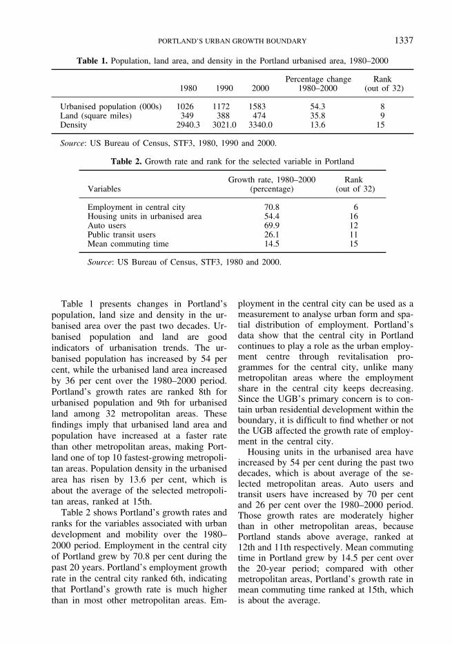
Figures 2–5 show the spatial distributionof housing units constructed during the1960s, 1970s, 1980s and 1990s. Approxi-mately 75 per cent of new housing units inthe 1960s were constructed inside the UGB.Clark County, Washington, accommodated15 per cent of the new housing units built inthe same period. The Portland metropolitanregion experienced rapid population (hous-

PORTLAND’S URBAN GROWTH BOUNDARY 1341

Figure 2. Housing units built, 1960–69. Key: 1 dot represents 50 housing units.

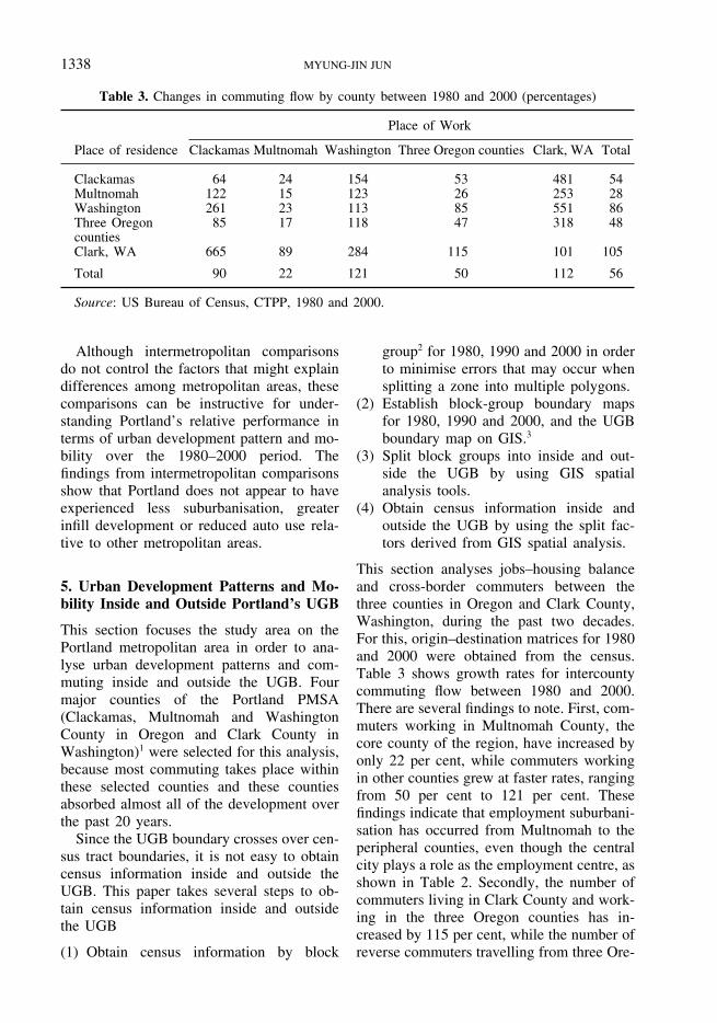
Figure 3. Housing units built, 1970–79. Key: 1 dot represents 50 housing units.

ing) growth during the 1970s, which resultedin doubling the number of new housing unitsconstructed during the 1960s. As shown inFigure 3, significant population suburbanisa-

tion started to take place towards ClarkCounty as well as to the south-east in the1970s. Total housing units constructed dur-ing 1980s declined by almost 60 000 units,

MYUNG-JIN JUN1342

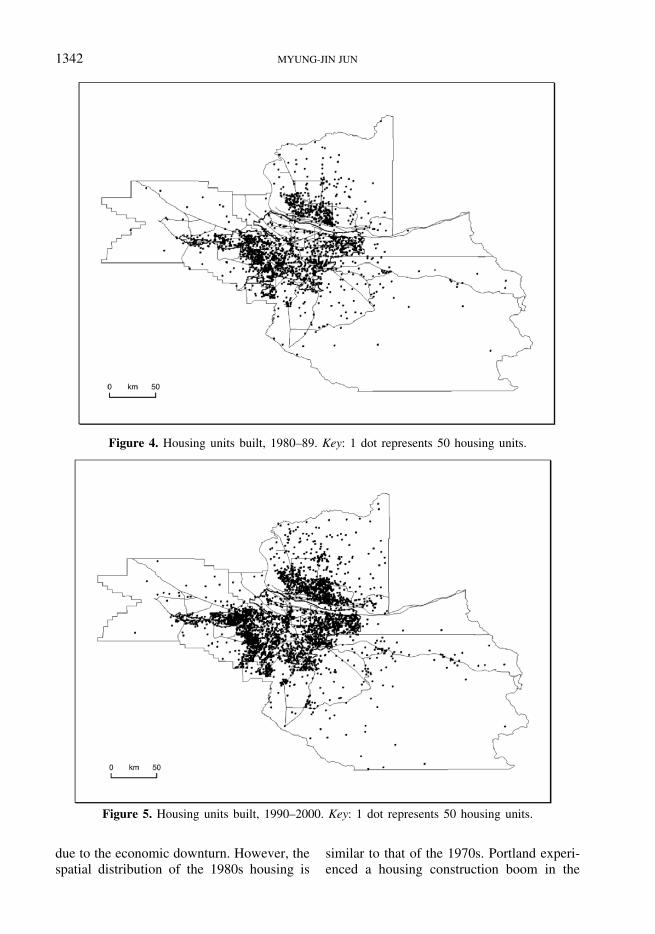
Figure 4. Housing units built, 1980–89. Key: 1 dot represents 50 housing units.

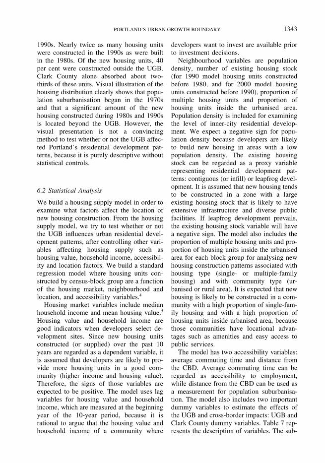
Figure 5. Housing units built, 1990–2000. Key: 1 dot represents 50 housing units.

due to the economic downturn. However, thespatial distribution of the 1980s housing is

similar to that of the 1970s. Portland experi-enced a housing construction boom in the

PORTLAND’S URBAN GROWTH BOUNDARY 1343

1990s. Nearly twice as many housing unitswere constructed in the 1990s as were builtin the 1980s. Of the new housing units, 40per cent were constructed outside the UGB.Clark County alone absorbed about two-thirds of these units. Visual illustration of thehousing distribution clearly shows that popu-lation suburbanisation began in the 1970sand that a significant amount of the newhousing constructed during 1980s and 1990sis located beyond the UGB. However, thevisual presentation is not a convincingmethod to test whether or not the UGB affec-ted Portland’s residential development pat-terns, because it is purely descriptive withoutstatistical controls.

6.2 Statistical Analysis

We build a housing supply model in order toexamine what factors affect the location ofnew housing construction. From the housingsupply model, we try to test whether or notthe UGB influences urban residential devel-opment patterns, after controlling other vari-ables affecting housing supply such ashousing value, household income, accessibil-ity and location factors. We build a standardregression model where housing units con-structed by census-block group are a functionof the housing market, neighbourhood andlocation, and accessibility variables.4

Housing market variables include medianhousehold income and mean housing value.5

Housing value and household income aregood indicators when developers select de-velopment sites. Since new housing unitsconstructed (or supplied) over the past 10years are regarded as a dependent variable, itis assumed that developers are likely to pro-vide more housing units in a good com-munity (higher income and housing value).Therefore, the signs of those variables areexpected to be positive. The model uses lagvariables for housing value and householdincome, which are measured at the beginningyear of the 10-year period, because it isrational to argue that the housing value andhousehold income of a community where

developers want to invest are available priorto investment decisions.

Neighbourhood variables are populationdensity, number of existing housing stock(for 1990 model housing units constructedbefore 1980, and for 2000 model housingunits constructed before 1990), proportion ofmultiple housing units and proportion ofhousing units inside the urbanised area.Population density is included for examiningthe level of inner-city residential develop-ment. We expect a negative sign for popu-lation density because developers are likelyto build new housing in areas with a lowpopulation density. The existing housingstock can be regarded as a proxy variablerepresenting residential development pat-terns: contiguous (or infill) or leapfrog devel-opment. It is assumed that new housing tendsto be constructed in a zone with a largeexisting housing stock that is likely to haveextensive infrastructure and diverse publicfacilities. If leapfrog development prevails,the existing housing stock variable will havea negative sign. The model also includes theproportion of multiple housing units and pro-portion of housing units inside the urbanisedarea for each block group for analysing newhousing construction patterns associated withhousing type (single- or multiple-familyhousing) and with community type (ur-banised or rural area). It is expected that newhousing is likely to be constructed in a com-munity with a high proportion of single-fam-ily housing and with a high proportion ofhousing units inside urbanised area, becausethose communities have locational advan-tages such as amenities and easy access topublic services.

The model has two accessibility variables:average commuting time and distance fromthe CBD. Average commuting time can beregarded as accessibility to employment,while distance from the CBD can be used asa measurement for population suburbanisa-tion. The model also includes two importantdummy variables to estimate the effects ofthe UGB and cross-border impacts: UGB andClark County dummy variables. Table 7 rep-resents the description of variables. The sub-

MYUNG-JIN JUN1344

Table 7. Description of variables

DescriptionVariable

Natural log of the existing housing stock at year t � 1LN Hstockt � 1

Natural log of population density at year t � 1LN Popdent � 1

Mid Incomet � 1 Median household income at year t � 1Mean Valt � 1 Mean housing value at year t � 1

Mean commuting timeMean TimeDist CBD Distance from CBDMulti HS r Ratio of multiple housing to total

Proportion of housing units located in urban area to totalUr HS rUGB Dummy UGB dummy (1 if within UGB, 0 otherwise)WA Dummy Washington State dummy (1 if within Washington, 0 otherwise)

Table 8. Regression analysis, 1980–90 (N � 1143)

T-valueVariable ProbabilityEstimate

0.0001Intercept � 13.17� 6.276916.45 0.0001LN Hstockt � 1 0.7066

0.0144LN Popdent � 1 � 2.45� 0.06985.37Mid Incomet � 1 0.00016.E-05

0.0001Mean Valt � 1 5.640.01643.86 0.0001Mean Time 0.0527

0.0001Dist CBD 7.924.60209.42Multi HS r 0.00011.9742

0.0093Ur HS r 2.610.50580.52UGB Dummy 0.60340.0817

WA Dummy 4.750.8215 0.0001

R2 � 0.434

script t-1 indicates the beginning year of themodel. For the 1990 model, t-1 refers to1980.

Tables 8 and 9 report runs of the standardregression model for 1990 and 2000. Asexpected, both median household incomeand mean housing value are positively re-lated to new housing units built. These vari-ables have the expected sign and arestatistically significant for both the 1990 and2000 models. Population density negativelyaffects new housing construction, while theexisting housing stock is positively related tonew housing provision. New housing is morelikely to be constructed in a zone with alower population density and with a largerhousing stock. This result implies that newhousing construction took place in the subur-ban area (low population density), but not by

means of leapfrogging residential develop-ment.

Another important finding is that the dis-tance from the CBD and mean commutingtime are positively related to new housingconstruction and statistically significant forboth models. This indicates that more hous-ing units are constructed as the zone locatesfarther away from the CBD, which supportsthe previous argument on population subur-banisation (Table 1). This also supports thefinding that more housing units are built inthe suburban area, where commuters havelonger travel times, than in the central city(Table 5).

The proportion of multiple housing unitsand proportion of housing units inside theurbanised area are both positively relatedwith new housing construction and are statis-

PORTLAND’S URBAN GROWTH BOUNDARY 1345

Table 9. Regression analysis, 1990–2000 (N � 1225)

Variable T-valueEstimate Probability

Intercept � 1.3118 0.0235� 2.270.0001LN Hstockt � 1 6.170.3023

� 9.2LN Popdent � 1 0.00010.36680.0058Mid Incomet � 1 2.762.E-05

4.41Mean Valt � 1 0.00018.E-06Mean Time 0.0404 3.59 0.0003

0.0001Dist CBD 10.15.5319Multi HS r 1.8528 8.88 0.0001

0.0001Ur HS r 10.622.1609UGB Dummy 1.480.2106 0.1387WA Dummy 6.931.0165 0.0001

R2 � 0.412

tically significant for both models. This sug-gests that new housing is more likely to bebuilt inside the urbanised area and in a zonewith more multiple housing. This finding canbe interpreted as an indication that the UGBencouraged compact development. However,the positive relation between new housingconstruction and the proportion of multiplehousing units seems to be affected not by theUGB, but by the spatial distribution of mul-tiple housing in Portland. According to thecensus, about 24.5 per cent in 1990 and 24.1per cent in 2000 of total multiple housingunits were located outside the UGB in Port-land. A similar interpretation can be appliedto the positive relation between the pro-portion of housing units inside the urbanisedarea and new housing construction. Censusdata revealed that 19.0 per cent in 1990 and23.4 per cent in 2000 of total housing unitsinside the urbanised area were located out-side the UGB.

The most important result from this analy-sis is that the UGB dummy variable is notstatistically significant for both the 1990 andthe 2000 models, implying that the UGB hadno impact on the location of new housingconstruction. Unlike the UGB, the ClarkCounty dummy variable is significant forboth models. Those results suggest that Port-land’s UGB had little influence on determin-ing the location of new housing construction,while Clark County attracted a significantamount of new housing construction during

the past 20 years. More importantly, theseresults suggest that the UGB diverted Ore-gon’s housing growth to Clark County, sincethe regression model controlled housing mar-ket, neighbourhood and accessibility vari-ables.

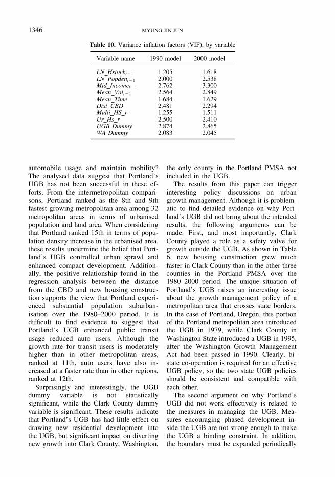
In a study of this kind, it is desirable toaddress the issues of multicollinearity andheteroscedasticity. A standard collinearity di-agnosis (Belsey et al., 1980) generated con-dition indices of 34.8 in 1990 and 48.2 in the2000 model, implying no multicollinearityproblem. In addition, the variance inflationfactor (VIF) is computed for each variable inorder to check multicollinearity (Table 10).As a rule of thumb, for standardised data, aVIF � 10 indicates harmful collinearity(Kennedy, 1985). None of variables in theregression model has a multicollinearityproblem, since the VIFs range from 1.2 to3.3 for both models. This study also tests forheteroscedasticity by applying the Breushch–Pagan (BP) test (Wooldridge, 2000, pp. 266–270). The null hypothesis of noheteroscedasticity is accepted for both stan-dard regression models.

7. Conclusions

This paper presents several analyses to an-swer various questions about Portland’sUGB that have been debated at great length:did Portland’s UGB control sprawl, curtail

MYUNG-JIN JUN1346

Table 10. Variance inflation factors (VIF), by variable

1990 modelVariable name 2000 model

1.205LN Hstockt � 1 1.6182.538LN Popdent � 1 2.000

2.762Mid Incomet � 1 3.3002.849Mean Valt � 1 2.564

Mean Time 1.6291.6842.294Dist CBD 2.481

1.255Multi HS r 1.5112.410Ur Hs r 2.500

UGB Dummy 2.8652.874WA Dummy 2.0452.083

automobile usage and maintain mobility?The analysed data suggest that Portland’sUGB has not been successful in these ef-forts. From the intermetropolitan compari-sons, Portland ranked as the 8th and 9thfastest-growing metropolitan area among 32metropolitan areas in terms of urbanisedpopulation and land area. When consideringthat Portland ranked 15th in terms of popu-lation density increase in the urbanised area,these results undermine the belief that Port-land’s UGB controlled urban sprawl andenhanced compact development. Addition-ally, the positive relationship found in theregression analysis between the distancefrom the CBD and new housing construc-tion supports the view that Portland experi-enced substantial population suburban-isation over the 1980–2000 period. It isdifficult to find evidence to suggest thatPortland’s UGB enhanced public transitusage reduced auto users. Although thegrowth rate for transit users is moderatelyhigher than in other metropolitan areas,ranked at 11th, auto users have also in-creased at a faster rate than in other regions,ranked at 12th.

Surprisingly and interestingly, the UGBdummy variable is not statisticallysignificant, while the Clark County dummyvariable is significant. These results indicatethat Portland’s UGB has had little effect ondrawing new residential development intothe UGB, but significant impact on divertingnew growth into Clark County, Washington,

the only county in the Portland PMSA notincluded in the UGB.

The results from this paper can triggerinteresting policy discussions on urbangrowth management. Although it is problem-atic to find detailed evidence on why Port-land’s UGB did not bring about the intendedresults, the following arguments can bemade. First, and most importantly, ClarkCounty played a role as a safety valve forgrowth outside the UGB. As shown in Table6, new housing construction grew muchfaster in Clark County than in the other threecounties in the Portland PMSA over the1980–2000 period. The unique situation ofPortland’s UGB raises an interesting issueabout the growth management policy of ametropolitan area that crosses state borders.In the case of Portland, Oregon, this portionof the Portland metropolitan area introducedthe UGB in 1979, while Clark County inWashington State introduced a UGB in 1995,after the Washington Growth ManagementAct had been passed in 1990. Clearly, bi-state co-operation is required for an effectiveUGB policy, so the two state UGB policiesshould be consistent and compatible witheach other.

The second argument on why Portland’sUGB did not work effectively is related tothe measures in managing the UGB. Mea-sures encouraging phased development in-side the UGB are not strong enough to makethe UGB a binding constraint. In addition,the boundary must be expanded periodically

PORTLAND’S URBAN GROWTH BOUNDARY 1347

to accommodate 20 years of growth. A goodexample of a strong growth control policy isSeoul’s Greenbelt. Seoul’s Greenbelt wasbeen designated in the Seoul metropolitanarea in 1976 and has remained in place fornearly 30 years, allowing no developmentwithin the Greenbelt. Although the Greenbeltremains intact due to the banning of privatedevelopment, achieving its primary goals, atight greenbelt policy in a rapidly growingmetropolitan area such as Seoul has someadverse effects: inner-city densification andleapfrog development (Bae and Jun, 2003).So a tight UGB policy can encourage com-pact development, but restrictive land useregulation like Seoul’s Greenbelt is both con-stitutionally impossible and politically be-yond reality in the US.

This paper initiates an active discussion onthe effects of Portland’s UGB and should notbe understood as an attempt to provide aconclusive end to the Portland UGB contro-versy. Diverse analyses are required to studythe overall effect of the UGB. Micro-levelanalysis, such as studying development pat-terns on a street or corridor within the UGBor analysing land use changes outside theUGB from agricultural and environmentallysensitive lands into urban land uses, wouldfurther contribute to an informed discussionanalysing the effects of Portland’s UGB. Dis-cussion arising from this paper should spurthese analyses and further study of UGBimpact.

Notes

1. These four counties had 93.3 per cent of totalpopulation of Portland PMSA in 2000.

2. Block, of course, is the smallest geographicalunit available in the census. However, it isnot possible to obtain block-level boundarymaps for 1980, 1990 and 2000 for the studyarea.

3. During the past two decades, the UGB haschanged almost three dozen times. Mostchanges were about 20 acres or less. Themost significant increase has occurred in1998 and 1999 by addition of about 4000acres, which is a 1.5 per cent increase of thetotal UGB. The UGB boundary map releasedby the Metro in 2000 was used for this

analysis because it is almost impossible toaccommodate all the boundary changes intothe analysis and, even though major changeswere incorporated, it is not expected to affectsignificantly the analysis results.

4. Since census information is aggregated data,it is not possible to build a behaviouralmodel, which considers both consumer hous-ing choices and developer site choices.

5. The model uses mean housing value insteadof median housing value because there is noinformation about median housing value inthe 1980 census.

References

BAE, C.-H. C. (2001) Cross-border impacts ofgrowth management programs: Portland, Ore-gon, and Clark County, Washington. Paperpresented at 17th Pacific Regional ScienceConference, Portland, OR.

BAE, C.-H, C. and JUN, M.-J. (2003) Counterfac-tual planning: what if there had been no green-belt in Seoul?, Journal of Planning Educationand Research, 22, pp. 374–383.

BELSLEY, D. A., KUH, E. and WELSCH, R. E.(1980) Regression Diagnostics. New York:John Wiley & Sons.

BRUECKNER, J. K. (2000) Urban sprawl: diagnosisand remedies, International Regional ScienceReview, 23(2), pp. 160–170.

COX, W. (2001) American dream boundaries: ur-ban containment and its consequences(www.gppf.org/pubs/analyses/2001).

DANIELS, T. (1999) When City and Country Col-lide: Managing Growth in the MetropolitanFringe. Washington, DC: Island Press.

DING, C., KNAAP, G. J. and HOPKINS, L. D. (1999)Managing urban growth with urban growthboundaries: a theoretical analysis, Journal ofUrban Economics, 46, pp. 53–68.

KENNEDY, P. (1985) A Guide to Econometrics,2nd edn. Cambridge, MA: The MIT Press.

KLINE, J. and ALIG, R. (1999) Does land useplanning slow the conversion of forest and farmlands, Growth and Change, 30, pp. 3–22.

KNAAP, G. K. (2000) The urban growth boundaryin metropolitan Portland, Oregon: research,rhetoric, and reality. Paper presented at theWorkshop on Urban Growth Management Poli-cies in the U.S., Japan, and Korea, Seoul Na-tional University, Seoul, Korea.

METRO (2002) Urban growth boundary: fre-quently asked questions (http://topaz.metro-re-gion.org).

NELSON, A. C. and DUNCAN, J. B. (1995) GrowthManagement: Principles and Practice.Chicago, IL: American Planning Association.

NELSON, A. C. and MOORE, T. (1993) Assessing

MYUNG-JIN JUN1348

urban growth management: the case of port-land, Oregon, the USA’s largest urban growthboundary, Land Use Policy, 10, pp. 293–302.

ONE THOUSAND FRIENDS OF OREGON (1991) Man-aging growth to promote affordable housing:revisiting Oregon’s Goal 10. Portland, OR:1000 Friends of Oregon.

PATTERSON, J. (1999) Urban growth boundaryimpacts on sprawl and redevelopment in Port-land, Oregon. Working Paper, University ofWisconsin–Whitewater.

RICHARDSON, H. W. and GORDON, P. (2001) Port-

land and Los Angeles: beauty and the beast.Paper presented at the 17th Pacific RegionalScience Conference, Portland, OR.

STALEY, S. R., EDGENS, J. D. and MILDNER, G. C.S. (1999) A line in the land: urban-growthboundaries, smart growth, and housing afford-ability. Policy Study No. 263, Reason PublicPolicy Institute.

WOOLDRIDGE, J. M. (2000) Introductory Econo-metrics: A Modern Approach. Cincinnati, OH:South-Western College Publishing.