Problem Set #3Geog 2000: Introduction to Geographic Statistics

Instructor: Dr. Paul C. Sutton

Due Tuesday Week #7 in LabInstructions: There are three parts to this problem set: 1) Do it by Hand Exercises (#’s 1 – 15). Do these with a calculator or by hand. Draw most of your figures by hand. Write out your answers either digitally or by hand. Start your answer to each numbered question on a new page. Make it easy for me to grade. 2) Computer exercises (#’s 16-18). Use the computer to generate the graphics and paste them into a digital version of this assignment while leaving room for you to digitally or hand write your responses if you so wish. 3) ‘How to Lie with Statistics’ Essay(s) (#’s 19-23). For this section, prepare a typed paragraph answering each question. Do not send me digital versions of your answers. I want paper copies because that is the easiest way for me to spill coffee on your assignments when I am grading them. All of the questions on these four problem sets will resemble many of the questions on the three exams. Consequently, it behooves you to truly understand – ON YOUR OWN – how to do these problems. This is a LONG problem set. Get started early.

Rosencrantz and Guildenstern are spinning in their graves.

Do it By Hand Exercises (i.e. Don’t Use A Computer)#1) Sampling Design

Usually it is too costly in terms of time, money, and/or effort to measure every item in a population (e.g. the length of all the bananas in the world, the average weight of 18 year old men in California, the fraction of defective light bulbs coming off an assembly line, etc). Consequently, we take a statistical approach to such problems by sampling a much smaller number from a population to make an inference about the parameters of a population. For the previous examples you could select 30 bananas and measure their respective lengths and estimate two parameters: The mean length of a banana (central tendency), and the standard deviation or variance of the lengths of those bananas (spread). The same parameters (mean, and variance) could be estimated for the weights of 18 year old Californian men. With the light bulbs the parameter you would be estimating is what fraction of the bulbs are defective. The quality of your estimates of these parameters depend profoundly on the quality of your sampling approach. Your sampling design must be ‘representative’ of the population you are trying to estimate parameters for. This usually requires ‘randomness’ of selection of your sample. Also, the confidence intervals about your parameter estimates tend to shrink as your sample size increases.

A) Define and provide an example of the following terms: Population, Sample, Parameter, Random Selection, Sampling Frame

A concrete example is a reasonable way to provide these definitions. Assume you are a campaign manager for a presidential candidate. You want to assess how you candidate stands with respect to actual voters. You can’t survey all of them (we have elections for that – pretty expensive). All the actual voters would be the population you would define. Human behavior being what it is you cannot really guarantee to sample from actual voters. Consequently you will develop a sampling frame which is often registered voters. The sampling frame is the pool of potential entities that can possibly be sampled. You may use various tricks to weight your actual sample to get at something like likely voters (demographic weightings, geographic weightings, etc.). You may or may not parse (aka stratify) your sampling frame to in essence weight your results; in any case, you will want to randomly sample from the stratified or not stratified entities in your sampling frame. Random sampling simply means that all entities in your sampling frame or strata of your sampling frame have an equal chance of being selected. Your sample is simply those entities that are actually selected and measured. The parameter you might be trying to estimate is the fraction (or percentage) of the population that intends to vote for your candidate. This has an actual and true value which will be ascertained on election day. You will make an estimate of that parameter using a statistic. Your estimate will tend to be more accurate the larger a sample size you use; however, many things can mess you up: 1) Your candidate could be caught on camera at a Ku Klux Klan rally between the time your survey is done and election day (that might reduce his popularity). 2) A military conscription or draft may be instituted which changes the voter turnout of young voters. Basically there are lots of ways that your estimate of the percentage of voters intending to vote for your candidate can be changed by the course of events. Nonetheless, these polls are more often than not pretty useful as is suggested by the fact that so many are still conducted.

B) Define and provide an example of the following sampling approaches: Simple Random Sampling, Stratified Random Sampling, Cluster Sampling, and Systematic sampling.

Simple Random Sampling: Every entity within the sampling frame has an equal probability of being selected for the sample.

Cluster Sampling & Stratified Sampling: Wikipedia again - Cluster sampling is a sampling technique used when "natural" groupings are evident in a statistical population. It is often used in marketing research. In this technique, the total population is divided into these groups (or clusters) and a sample of the groups is selected. Then the required information is collected from the elements within each selected group. This may be done for every element in these groups or a subsample of elements may be selected within each of these groups. Elements within a cluster should ideally be as heterogeneous as possible, but there should be homogeneity between cluster means. Each cluster should be a small scale representation of the total population. The clusters should be mutually exclusive and collectively exhaustive. A random sampling technique is then used on any relevant clusters to choose which clusters to include in the study. In single-stage cluster sampling, all the elements from each of the selected clusters are used. In two-stage cluster sampling, a random sampling technique is applied to the elements from each of the selected clusters. The main difference between cluster sampling and stratified sampling is that in cluster sampling the cluster is treated as the sampling unit so analysis is done on a population of clusters (at least in the first stage). In stratified sampling, the analysis is done on elements within strata. In stratified sampling, a random sample is drawn from each of the strata, whereas in cluster sampling only the selected clusters are studied. The main objective of cluster sampling is to reduce costs by increasing sampling efficiency. This contrasts with stratified sampling where the main objective is to increase precision. One version of cluster sampling is area sampling or geographical cluster sampling. Clusters consist of geographical areas. Because a geographically dispersed population can be expensive to survey, greater economy than simple random sampling can be achieved by treating several respondents within a local area as a cluster. It is usually necessary to increase the total sample size to achieve equivalent precision in the estimators, but cost savings may make that feasible. In some situations, cluster analysis is only appropriate when the clusters are approximately the same size. This can be achieved by combining clusters. If this is not possible, probability proportionate to size sampling is used. In this method, the probability of selecting any cluster varies with the size of the cluster, giving larger clusters a greater probability of selection and smaller clusters a lower probability. However, if clusters are selected with probability proportionate to size, the same number of interviews should be carried out in each sampled cluster so that each unit sampled has the same probability of selection. Cluster sampling is used to estimate high mortalities in cases such as wars, famines and natural disasters. Stratified sampling may be done when you are interested in a sector of the population that might be small (say left-handed horseback riders). A simple random sample would not produce many subjects that were left-handed horseback riders. So, you can stratify your sample and increase the number of left-handed horseback riders that you sample to allow for statistical comparisons. Systematic Sampling: An example is taking every 50th phone number in the phone book or every 5th customer that walks into a Barnes and Nobles Bookstore. It is supposedly a structured way of getting at a random sample but has some pitfalls associated with potential periodicity in the ‘stream’ of your sampling frame.

C) Explain the two important aspects of Simple Random Sampling: Unbiasedness and Independence

The property of unbiasedness simply means that the mechanism or procedure by which you select entities from your sampling frame should not mess with the equal probability of selection principle (this is of course assuming your sampling frame is representative of the population you are trying to estimate parameters of – See Part ‘D’). A classic example is asking for volunteers. People who volunteer for things are a biased sample of human subjects in many many ways. Suppose you are sampling fish in a lake. If you are catching them the old-fashioned way (probably not a good idea) with a fishing hook – you probably won’t sample the fish whose mouth is too small to get around the hook or the older wiser fish that tend not to get caught. These are kinds of bias.

The property of independence manifests in several ways. In terms of sampling – the selection of one entity should not change the probability of any of the other entities in the sampling frame from being selected. Also, knowing the value of the measurement of a sampled entity should not inform you of the value of the measurement of any prior or subsequently selected entities of your sample.

D) Suppose you wanted to estimate the fraction of people of voting age in Colorado that believe the landmark Supreme Court decision regarding abortion (Roe v. Wade) should be overturned. (BTW: An interesting factoid I discovered in the Literature review for my Master’s Thesis was this – Only 30% of American adults could answer the question: “Roe vs. Wade was a landmark Supreme Court decision regarding what?”). You use all the names and phone numbers in all the yellow page phone books of the state. You randomly sample 1,000 people from this these phonebooks and ask them if they want Roe v. Wade overturned. Is this sampling approach a good one? What is the sampling frame? Is this an unbiased approach to sampling? Explain why or why not.

No matter how carefully you take this approach you probably have some serious bias in your sample. This is probably not a good sampling approach. The sampling frame is people who have phone numbers in Colorado phone books. This is probably biased because many people don’t have land lines anymore and cell phone numbers don’t show up in phone books. One way this is almost definitely biased is that it undersamples young people and oversamples older folks. Also, some adults don’t have any phones at all. This cell phone issue is becoming increasingly problematic for polling enterprises such as Pew and Gallup.

0 2 4 6 8 10 12 14 16 18

100.0%99.5%97.5%90.0%75.0%50.0%25.0%10.0%2.5%0.5%0.0%

maximum

quartilemedianquartile

minimum

16.00016.00015.00013.00010.5009.0007.0005.2002.5502.0002.000

QuantilesMeanStd DevStd Err Meanupper 95% Meanlower 95% MeanN

9.0495052.90646260.28920389.62327718.4757328

101

Moments

Bin

Distributions

#2) Condom manufacturing as a Bernoulli Trial

Suppose you start a condom manufacturing company. You have a method to test whether or not there are holes in your condoms (clearly this is something you might want to minimize). You have a machine that produces condoms for which you can control various settings. Suppose you test every one of your first batch of 10,000 condoms produced by this machine and 931 of them ‘fail’ the hole test.

A)Take a statistical approach to characterize the ‘effectiveness’ of your condoms based on your test results. Define your population and unknown parameter(s); find a statistic that estimates this parameter (an estimator) and the theoretical sampling distribution, mean, and standard deviation of this estimator; and use the data above as a random sampling of your product; finally, report and interpret your results and the statistical or sampling error associated with it.

The parameter I am trying to estimate is the fraction of the condoms that my machine produces that either do or don’t have holes in them. The population is all the condoms that my machine produces (this assumes that the defect rate is constant over time – probably not a good assumption but we’re going with it for the sake of simplicity). This problem is essentially identical to the Bernoulli Tack Factory problem in The Cartoon Guide. The statistic that estimates the parameter is given by: p^ = x / n , where ‘x’ is the number of condoms with holes (931), and ‘n’ is the size of the sample (10,000). Thus your estimate of the ‘defect rate’ of your condom machine is 9.31%.For large sample sizes the sampling distribution of p^ will be approximately normal with mean equal to ‘p’ (the true population parameter value) and the standard deviation (σ aka sigma) is given by: σ = (p*(1-p)1/2 / (n)1/2 (which in this case is estimated at .0029) . Since 10,000 is pretty dang large we can say with reasonable confidence that p^ is close to 9.31%.How close? Well we can say that there is a 68% chance that the range 9.31 +or- 0.21%(e.g. 9.1% - 9.52%) contains the true parameter value ‘p’. We can say with 95% confidence that the range 9.31 +or- 0.42 (e.g. 8.89% - 9.74%) contains the true parameter value ‘p’.

A) How will your estimate of the failure rate of your condoms change if you only sampled 100 condoms?

The estimate remains the same at 9.31%; however, the confidence intervals increase (get larger) because of the smaller sample size. In this case the 68% range is 9.31 +or- 2.1% and the 95% confidence range is 9.31 +or- 4.2%.

B) Explain why your actual ‘condom failure’ in real use (e.g. someone gets pregnant) might be significantly higher or lower than your estimates of the fraction of your product that has a hole in it.

It could be higher if people don’t use the condom correctly. It could be lower because some people are infertile and the condom does not matter.

C) Suppose you made 100 condoms 1,000 times and estimated ‘p-hat’ 1,000 times (once for each batch of 100). What would the probability mass function (pmf) look like for ‘p-hat’ where ‘’p-hat’ = # of condoms with holes / 100?

It would look somewhat like the chart on the right. This was a random instantiation so the bars are not exact as probabilities. The highest bar is for the value of 9 and the probabilities are symmetric about 9.

0 1 2 3 4

100.0%99.5%97.5%90.0%75.0%50.0%25.0%10.0%2.5%0.5%0.0%

maximum

quartilemedianquartile

minimum

4.00004.00003.00002.00001.00001.00000.00000.00000.00000.00000.0000

QuantilesMeanStd DevStd Err Meanupper 95% Meanlower 95% MeanN

0.9702970.92147110.09168981.152207

0.7883871101

Moments

Bin

Distributions

850 900 950 1000 1050

100.0%99.5%97.5%90.0%75.0%50.0%25.0%10.0%2.5%0.5%0.0%

maximum

quartilemedianquartile

minimum

1039.01039.01025.0963.6949.0926.0911.5892.4874.6847.0847.0

QuantilesMeanStd DevStd Err Meanupper 95% Meanlower 95% MeanN

929.1188130.9416513.0788093935.22708923.01054

101

Moments

Bin

Distributions

D) What if your batches were of size N= 10; how would the pmf change? What if your batch sizes were N=10,000; how would the pmf change?

Now, with a sample size of 10 there is a good chance you won’t catch any failed condoms because only about 9% of them fail. The only possible numbers you can get are the 11 possibilities from 0 – 11. The probability of finding more than 4 failures are so low that a random generation will rarely have any values higher than 4. 100 randomly generated Bin(10, 0.931)

By sampling 10,000 you get finer resolution with respect to the sampling distribution of your mean. This gives you a clearer picture of both your mean and the spread about your mean because of the increased sample size. Again, the histogram at right is simply a random generation of 100 numbers from a Bin (10,000, 0.0931) random variable.

100 randomly generated Bin(10,000, 0.0931)

E) How does Sample Size improve parameter estimation of ‘p’?

From the figures above you can see that with a sample size of 10 your estimates become pretty coarse and your estimates will be 0%, or 10%, or 20%, or 30%, or even 40% (the probability of them being higher is non-zero but vanishingly small). With a sample size of 10,000 your estimates will almost always lie in the 8.5% to 10.5% range. This is a much tighter estimate. In fact, the tightness (confidence interval) of your estimate increases with the square root of your sample size.

F) What assumptions are you making with respect to estimation of ‘p’?

You are assuming that your condom making machine has a constant failure rate during production. You are deciding that your hole measuring test is perfect and that holes are the only kind of ‘defect’ you want to measure.

H) Provide the formulas (i.e. estimators) for your estimates of both ‘p’ and σ(p).

‘p’ is simply estimated by: # of failures / # of condoms sampled for failureSigma is simply estimated with the standard deviation of a binomial random variable:

σ = (p*(1-p)1/2 / (n)1/2

I) Use the idea of ‘Sampling Error’ to explain exactly what it would mean to have an estimate of p (i.e. ‘p-hat’) = 0.67 and an estimate of σ(p) = .07.

When you estimate ‘p’ using ‘p-hat’ = x / N and get 0.67 you know that you are likely close but not exactly identifying ‘p’. Your σ(p) = .07 gives you an idea of how close you are. If N is large and you can approximate with normality then you can say the following: I have a 68% confidence that the interval 0.60 to 0.74 contains the true ‘p’. I can say with 95% confidence that the interval 0.54 to 0.81 contains the true value of ‘p’. (e.g. your sample mean plus or minus one standard deviation and your sample mean plus or minus two standard deviations).

#3) Black Velvet, Wildfire, and Mr. Ed were not ordinary horses

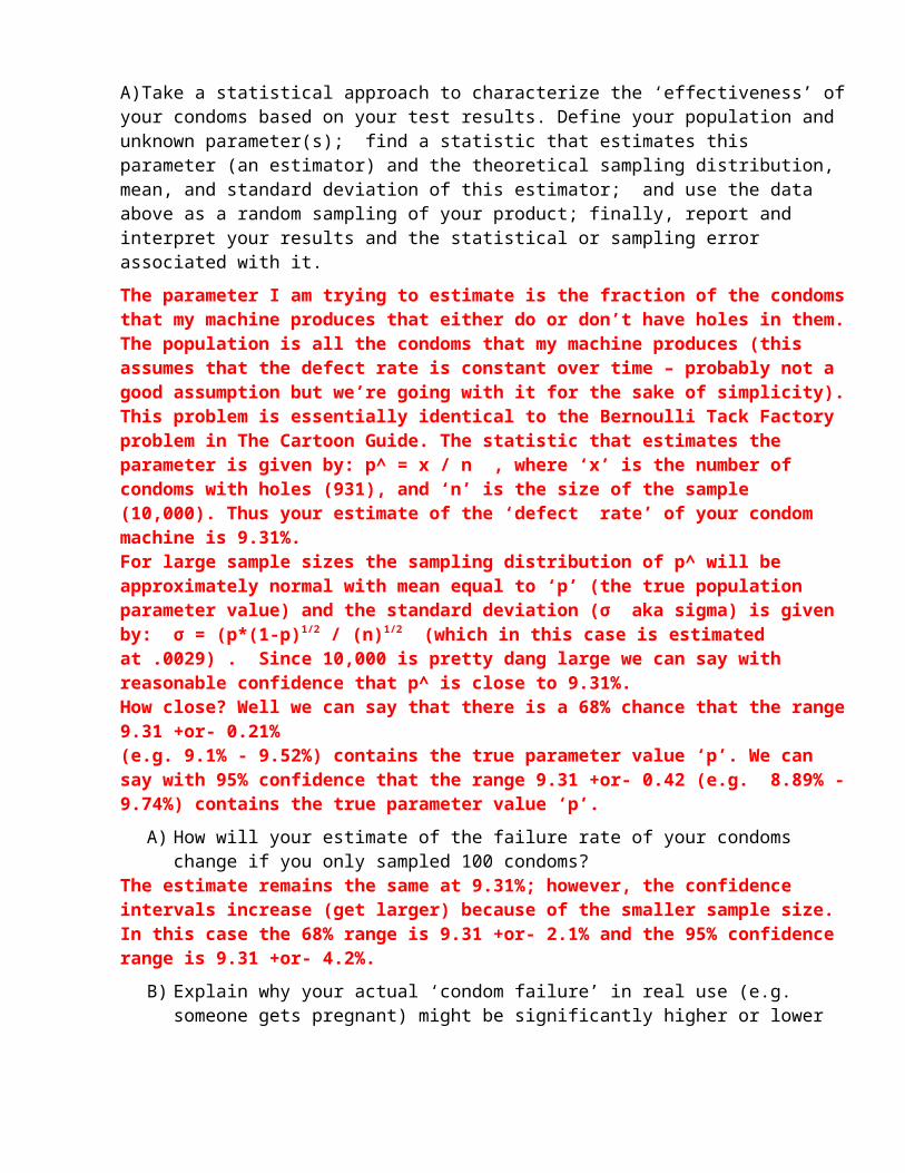
Let’s Consider ordinary horses. Consider the following random variable: The mass of a randomly selected adult horse (over 1 year old) in the United States. Assume there are exactly 1,000,000 horses in the U.S. Assume the true average mass of these horses is 530 kg. Assume the true variance of the masses of these horses is 6,400. Suppose you weigh 100 randomly selected horses and calculate a mean of 520 kg and a variance of 5,625.

A) What is the true population mean (μ)? 530 kgB) What is the true population variance (σ2)? 6,400C) What is the true population standard deviation (σ)? 80D) What was your estimate of the mean (x-bar)? 520 kg E) What was your estimate of the variance (s2)? 5,625F) What probability distribution function (pdf) would best describe

A sampling distribution of the mean for this random variableAssuming a sample size of N = 100? N(530, 8) or N(520, 75)

G) What pdf would best characterize the sampling distribution of The mean of this random variable if the sample size was N = 10? N(530, 25.3) or N(520, 42.2)H) What estimators did you use for μ and σ2 ?

a) μ was estimated with Xbar = Sum of weights of all sampled horses / # horses sampledb) σ2 was estimated with s2 = [(weight of each horse – avg weight of sampled horses)2/99]1/2

I) Did your estimates of these population parameters seem reasonableOr are they wrong enough to suggest your sampling methodologyWas biased? Explain.

Our sample size was 100. Our estimate of the mean was 10 kg low. For a sample size of 100 using the known population parameters we would expect a sampling distribution of the mean to be distributed approximately N(530, 8). So, by being off by 10 we were more than 1 standard deviation below the mean (1.25 to be exact). This is a little unusual but not terribly unusual. Certainly not outside of the 95% Confidence range.

#4) The Central Limit Theorem

A) Summarize the Central Limit Theorem in your own words

When you sample any numeric random variable be it discrete or continuous and regardless of its probability distribution function, the sampling distribution of that mean will be distributed normally around the true population mean with a standard deviation that is the true standard deviation divided by the square root of your sample size (e.g Xbar is distributed N(μ, σ/(n1/2) ).

If you don’t really get this check out some cool java applets on the web to demonstrate:http://wise.cgu.edu/sdmmod/sdm_applet.asphttp://www.ruf.rice.edu/~lane/stat_sim/sampling_dist/

B) Given the pdf of a continuous random variable that looked like the figure Below w/ known μ = 100 and known σ2 = 25 , what would the sampling Distribution of this distribution’s mean look like for samples of N = 49?

The mean of this random variableWill be distributed as a N(100, 5/7) or N(100, .714)

C) Given the pdf of a continuous random variable that looked like the figure Below w/ known μ = 100 and known σ2 = 25 , what would the sampling Distribution of this distribution’s mean look like for samples of N = 49?

The mean of this random variableWill be also be distributed as a N(100, 5/7) or N(100, .714)

#5) William Gosset, The Guinness Brewery, and the Student’s ‘t’ distribution

The student’s ‘t’ (aka ‘t’ distribution of ‘t-test’ fame) looks a lot like the standard Normal (aka N(0,1) or ‘Z’) distribution. It looks very similar, symmetric, bell shaped etc. but it’s tails are a little ‘fatter’. Explain in your own words the student’s ‘t’ distribution. In your explanation provide a mathematical formula for the ‘t’ distribution, define and explain it’s parameter or parameters, and answer the following questions: 1) A ‘t’ distribution with how many degrees of freedom is identical to a N(0,1) distribution? And 2) Is the ‘t’ distribution more leptokurtic or platykurtic than the normal distribution?

From Wikipedia - The Student's t-distribution (or also t-distribution), in probability and statistics, is a probability distribution that arises in the problem of estimating the mean of a normally distributed population when the sample size is small. It is the basis of the popular Student's t-tests for the statistical significance of the difference between two sample means, and for confidence intervals for the difference between two population means. The Student's t-distribution is a special case of the generalised hyperbolic distribution. The derivation of the t-distribution was first published in 1908 by William Sealy Gosset, while he worked at a Guinness

Brewery in Dublin. He was prohibited from publishing under his own name, so the paper was written under the pseudonym Student. The t-test and the associated theory became well-known through the work of R.A. Fisher, who called the distribution "Student's distribution". Student's distribution arises when (as in nearly all practical statistical work) the population standard deviation is unknown and has to be estimated from the data. Textbook problems treating the standard deviation as if it were known are of two kinds: (1) those in which the sample size is so large that one may treat a data-based estimate of the variance as if it were certain, and (2) those that illustrate mathematical reasoning, in which the problem of estimating the standard deviation is temporarily ignored because that is not the point that the author or instructor is then explaining.

The real mathematical formula for the ‘t’ is pretty scary andUgly (see formula to the right). The upside-down ‘L’ thingy is a greek letter Gamma and is another kind of probability distribution.The easier way to think about ‘t’ is summarized below as it related to a normal distribution.

Suppose we have a simple random sample of size n drawn from a Normal population with mean and standard deviation . Let denote the sample mean and s, the sample standard deviation.

Then the quantity

 

has a t distribution with n-1 degrees of freedom. Note that there is a different t distribution for each sample size, in other words, it is a class of distributions. When we speak of a specific t distribution, we have to specify the degrees of freedom. The degrees of freedom for this t statistics comes from the sample standard deviation s in the denominator of equation 1. The t density curves are symmetric and bell-shaped like the normal distribution and have their peak at 0. However, the spread is more than that of the standard normal distribution. This is due to the fact that in formula 1, the denominator is s rather than . Since s is a random quantity varying with various samples, the variability in t is more, resulting in a larger spread. The larger the degrees of freedom, the closer the t-density is to the normal density. This reflects the fact that the standard deviation s approaches for large sample size n. You can visualize this in the applet below by moving the sliders. (http://www-stat.stanford.edu/~naras/jsm/TDensity/TDensity.html)

A ‘t’ distribution with ann infinite number of degrees of freedom is the same as a normal distribution. For practical purposes they are virtually indistinguishable at that seemingly magical number of 30.

A ‘t’ is more ‘leptokurtic’ than the normal which means it is ‘peakier’ with fatter tails.

#6) Dream Job: Logistical Statistician for Marborg Disposal - NOT!

Suppose you are working for a trash hauling company. Your trucks can hold 10,000 lbs of trash before they are both unsafe and illegal to drive. You randomly sample 30 of your customers and get the following values for the mass of their trash.

55 45 110 122 44 7387 89 67 145 38 9544 23 36 88 59 7258 67 38 56 28 8422 99 78 78 89 103

A) Estimate the mean and the 95% Confidence Interval for the mean amount of trash (in lbs) your average customer produces in a given week. Interpret your result.

69.73 + or – 1.96 * 30.12 lbs (e.g. the 95% C.I. is 9.49 lbs to 129.97 lbs)

B) How many customers would you schedule for each truck if you wanted to be 99% confident that any given truck would not exceed it’s weight limit? Note #1: When you add random variables (see pp 68-71 in Cartoon Guide) the variances add also. Note #2: Is this a one-tailed or two-tailed test?

I did not see a simple way to do this. My calculations (see excel spread sheet below) suggest the ‘tipping point’ was going from 131 to 132 customers.

Mean Variance 2.33 Sigma 99% CI # custs69.7 908.3 70.2 139.9 1.0

139.5 1816.6 99.3 238.8 2.0209.2 2724.9 121.6 330.8 3.0278.9 3633.2 140.4 419.4 4.0348.7 4541.5 157.0 505.7 5.0418.4 5449.8 172.0 590.4 6.0488.1 6358.1 185.8 673.9 7.0557.8 7266.4 198.6 756.5 8.0627.6 8174.7 210.7 838.2 9.0697.3 9083.0 222.1 919.4 10.0

. . . . .

. . . . .

. . . . ..=69.73 * # custs .=70.18 * # custs .=2.33*sqrt(Variance) .=mean + 2.33 Sigma .=Cell above + 1

. . . . .

. . . . .

. . . . .8855.7 115354.1 791.4 9647.1 127.08925.4 116262.4 794.5 9719.9 128.08995.2 117170.7 797.6 9792.7 129.09064.9 118079.0 800.6 9865.5 130.09134.6 118987.3 803.7 9938.4 131.09204.4 119895.6 806.8 10011.1 132.0

This should be a one-tailed test because you don’t care about having too low a weight in the truck. Consequently the z-score you want to use is 2.33 (the area of the standard normal

under the curve from +2.33 standard deviations to infinity is 0.0099 ~ 0.01). 2.33 * 30.12 = 70.2. Note the first number under the 2.33 sigma column in the table above. Otherwise you

have to keep adding means and variance until you get to 10,000 lbs for the 99% edge.

C) What kind of geographic and socio-economic-demographic information might suggest you tweak the # of customers per truck on a route-based basis in order for You to be most efficient? Also, do you think this statistical approach is really Reasonable for a trash hauling company?

This is probably not a reasonable approach. Apartments and Condos might have less trash. Older folks might have less trash. Families and people with big yards might have more trash. Socio-economic-demographic variables like these will manifest non-randomly in space which should help you optimize. Basically you will probably use empirical experience as your guide rather than some pointy-headed statistical analysis for a problem like this.

#7) Dead Men Tell No Tales (reference to ideas in a book: The Black Swam: The impact of low probability events)

Suppose over the years you meet 100 people who have opinions about passing cars by driving over the double yellow lines. Seventy of them think it’s crazy. Thirty claim they do it all the time and think its fine. How might this be a biased sample?

The dead people that ‘learned’ the hard way that passing over double yellow lines are not around to contribute to your sample. This is definitely a bias. In fact if their ghosts could come and tell tales it might change people’s minds.

#8) Alpha Inflation and Stockbroker Scams?

A stockbroker identifies 2,000 wealthy potential customers and sends them a newsletter telling ½ of them to buy stock ‘X’ and the other half to sell stock ‘X’. Stock ‘X’ then goes up. He then sends another newsletter to the ½ he told to by stock ‘X’. He sends 500 of them advice to buy stock ‘Y’ and sell advice to the other 500. He keeps doing this until he is down to about 10 or so customers and moves in for the kill. ‘Look at what a track record I have?’ etc. Google the statistical concept of ‘alpha inflation’ and relate it to this story and Explain. (An interesting book by Nicholas Nassim Taleb called: The Black Swan: The high impact of low probability events explores these ideas in many interesting ways).

Alpha inflation is basically the idea that if you are using a 95% confidence standard you will be wrong about ‘seeing significance’ 5% of the time. So if you do 20 statistical tests with a 95% Confidence standard, on average, one of them will show up significant if ALL of them really are not significant. This scam stockbroker is doing just that. He winnows down his potential customers on this sort of alpha inflation based principle. If his final ‘sucker set’ is 5% of his original mailing list this is perhaps more clear.

#9) Capital Crimes and Type I and Type II Errors

Imagine a murder trial. The defendant may or may not be guilty. The jury may or may not convict him or her. What are all the possibilities? Make an analogy between these possibilities and a typical statistical test involving hypothesis testing and explain type I and Type II error. Be sure to incorporate α and β into your answer.

The four possible situations in the murder trial are: 1) Innocent Person found guilty; 2) Innocent person found innocent; 3) Guilty person found innocent; and 4) Guilty person found guilty. The analyogy to Type I and Type II error is fairly straightforward if we consider ‘Innocent until proven guilty’ as analogous to the Null Hypothesis. Thus 1) Innocent person found innocent is like failing to reject the Null Hypothesis (No error made with probability equal to 1- α ); 2) Innocent person found guilty is like Type I error and has the probability equal to α ; 3) A guilty person found guilty (e.g. rejecting the null hypothesis correctly has probability 1 – β and is not an error); 4) A guilty person found innocent is analogous to Type II error and has probability β.

#10) Hypothesis Testing and flipping a Bogus (?) Coin?

Suppose someone hands a strange looking coin to you and claims it has a 50 / 50 chance of landing heads or tails (i.e. it’s a ‘fair’ coin). Create a Null Hypothesis (H0) and an Alternative Hypothesis (Ha) for this claim and test the coin with 10 flips. What will your 95% confidence decision rule be (i.e. what results of this experiment will suggest that you reject the Null Hypothesis)?

H0: P(‘heads’) = P(‘tails’) = .5Ha: P(‘heads’) not equal P(‘tails’)

The table on the right shows the probability of rolling each of possible number of heads in the flipping of a ‘fair’ coin ten times. At the 95% confidence level you can say that 0, 1, 9, or 10 heads is ‘too weird’ to consider the coin fair. This is a two-tailed test so you have to add all the probabilities on both ends of the distribution. If you went to a 99% confidence level you would only reject the null with 0 or 10 heads.

#11) Wetlands, Wal-Mart, and Weasels

Suppose Wal-Mart had to pave over a valuable wetland to make room for a new Super-Store and associated parking lot. In obtaining the permit the city planners insisted that Wal-Mart create twice as much wetland in two other locations. One criteria for assessing the ‘ecological quality’ of the ‘created’ wetlands is to measure the population density of snails in particular habitats within the new wetlands. The ‘standard’, based on the previously existing wetland and several others is 30 snails per square meter (μ), with a variance (σ2) of 100. Wal-Mart invites you out to the two wetlands they have created and you do a snail survey of 30 1x1 meter quadrats in each wetland. Your data is below:

Wetland ‘A’: 42, 36, 40, 29, 45, 39, 28, 30, 32, 28, 39, 19, 21, 44, 27, 28, 51, 27, 34, 7, 61, 37, 31, 37, 33, 20, 33, 51, 23, 24

Wetland ‘B’: 0, 14, 9, 0, 27, 33, 6, 7, 10, 14, 8, 5, 2, 22, 12, 10, 18, 5, 30, 6, 18, 7, 8, 17, 17, 1, 28, 0, 4, 11

A) Do either of these wetlands meet the standard with 95% Confidence? Explain

For this we will use a z-test although to be truly rigorous a t would be slightly more appropriate but we do have a sample size of 30 which is fairly large. In any case, with this particular data the conclusions would be the same using a ‘z’ or a’t’.

Adapted From Wikipedia - In order for the Z-test to be reliable, certain conditions must be met. The most important is that since the Z-test uses the population mean and population standard deviation, these must be known (in this case they are given as known – e.g. the mean and standard deviation of snail population derived from the obliterated wetland and others). The sample must be a simple random sample of the population. If the sample came from a different sampling method, a different formula must be used. It must also be known that the population varies normally (i.e., the sampling distribution of the probabilities of possible values fits a

standard normal curve) – (we don’t test for this but it does look suspect for Wetland ‘B’). Nonetheless, if it is not known that the population varies normally, it suffices to have a sufficiently large sample, generally agreed to be ≥ 30 or 40. In actuality, knowing the true σ of a population is unrealistic except for cases such as standardized testing in which the entire population is known. In cases where it is impossible to measure every member of a population it is more realistic to use a t-test, which uses the standard error obtained from the sample along with the t-distribution.The test requires the following to be known:σ (the standard deviation of the population) μ (the mean of the population) x (the mean of the sample) n (the size of the sample) First calculate the standard error (SE) of the mean:

The formula for calculating the z score for the Z-test is as follows:

Finally, the z score is compared to a Z table (aka A standard Normal Table), a table which contains the percent of area under the normal curve between the mean and the z score. Using this table will indicate whether the calculated z score is within the realm of chance or if the z score is so different from the mean that the sample mean is unlikely to have happened by chance.

0 10 20 30 40 50 60 70

100.0%99.5%97.5%90.0%75.0%50.0%25.0%10.0%2.5%0.5%0.0%

maximum

quartilemedianquartile

minimum

61.00061.00061.00050.40039.25032.50027.00020.1007.0007.0007.000

QuantilesMeanStd DevStd Err Meanupper 95% Meanlower 95% MeanN

33.210.9588572.000804437.29210529.107895

30

Moments

Wetland A

Distributions

-5 0 5 10 15 20 25 30 35

100.0%99.5%97.5%90.0%75.0%50.0%25.0%10.0%2.5%0.5%0.0%

maximum

quartilemedianquartile

minimum

33.00033.00033.00027.90017.2508.5004.7500.1000.0000.0000.000

QuantilesMeanStd DevStd Err Meanupper 95% Meanlower 95% MeanN

11.39.41074221.718158614.8140297.7859711

30

MomentsWetland B

Distributions

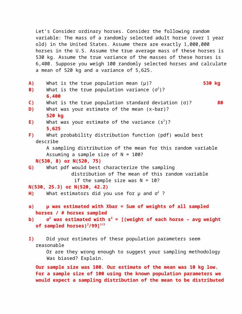
Wetland ‘A’: mean 33.2 s.d 10.96 Wetland ‘B’”: mean 11.3 s.d. 9.41

For wetland ‘A’: For wetland ‘B’: = _10__ = .33 (for both wetlands because we

30 use the ‘known’ population σ )

33.2 – 30 11.3 - 30Zwet’A’ = __________ = 9.7 Zwet’B’ = _________ = -56.7

.33 .33The ‘p’ values of these z-scores are: Zwet’A’ (9.7) = .0000 (beyond table)

And Zwet’A’ (-56.7) = .9999 (beyond table)Thus we conclude Wetland ‘A’ does have enough snails and Wetland ‘B’ does not. We can be confident of this at the 99% confidence level assuming the sampling methodology in the field was appropriate.

B) Are the tests you are conducting 1–tailed or 2-tailed?

This is a one-tailed (and One Sample) test because you are only concerned if there are more than enough snails. You are only testing that there are more than 30 snails per quadrat.And you are assuming a known population mean and variance.

C) What is better to use in this case a ‘t’ distribution or a normal?

Technically this is best done as a ‘t’-test. However if you do it as a ‘t’ you’ll come to the same conclusions with this data. The fact that the sample size was 30 for both Wetland ‘A’ and Wetland ‘B’ makes using a Z-table pretty safe.

#12) Reading the Standard Normal Table revisited…

A) For what values of ‘Z’ (assume they are equal with one being negative and the other positive) will the white area under the curve depicted below be equal to 0.95?

For values of + 1.96 and -1.96. If you look on standard normalTable you will find that the table value of Z = 1.96 is 0.025.

B) How does this value of ‘Z’ relate to the creation of 95% Confidence Intervals? Explain.

Well, 95% of the area under the standard normal curve exists under the x-axis from -1.96 to +1.96. So, if you are measuring/generating/drawing from a random variable that is appropriately modeled by a standard normal – 95% of the time it will occur withing this interval.

C)What would ‘Z’ have to be for the same area to be equal to 0.99?

On the standard normal table you will be looking for the z-score that has an α value of .005. This occurs between 2.57 and 2.58. Thus if you integrate the standard normal from -2.57 to + 2.57 you’ll get a value very close to 0.99.

D) The dark area on the figure below spans the N(0,1) curve from a value of 0 to 1.33. What is the area of this dark space?

An easy way to think about this is to simply realize thatThe value from 0 to ∞ is simply 0.5 (one half). Thus weCan simply subtract the area from 1.33 to ∞ (which is .0918 By the way). Thus the blue area is:

0.5 - .0918 = 0.4082

E) What is the area of the curve from Z = 1.5 to infinity as depicted in the image below?

Z = 1 .5

This is a simple read off the standard normal table: 0.0668

F) What is the area of the curve from Z = 1 to Z = 2 as depicted in the image below?

This is a simple difference between two simple reads off a standard normal table:

0.1587 – 0.0228 = 0.1359

#13) Polls, Pols, and the Binomial Distribution

Suppose the campaign committee of Barack Obama polled 1,000 registered Democrats one week prior to his primary election against Hillary Clinton in Texas in late February 2008. The survey question simply was: “Who will you vote for, Barack Obama or Hillary Clinton in next week’s presidential primary?”. Suppose 547 people said ‘Barack Obama’.

A) The true fraction of registered democrats that would state in a phone survey on that day that they would vote for Barack Obama is unknown (an unknown population parameter that could only be ascertained by asking every registered democrat in the state of Texas – we’ll get to know that value on election day). However, this survey has produced an estimate of that fraction. What is the estimate in percentage terms and what is your 95% Confidence Interval regarding that estimate? Explain. Show your formulas and calculations.

p-hat = X / N = 547 / 1,000 = .547 -> 54.7%

and, σ (p-hat) is given by

σ (p-hat) = (p*(1-p))1/2 / (n)1/2 = (.547*.453) 1/2 / (1000)1/2 = .00784

So – going with normality assumption : 95% C.I. is 54.7 +/- 0.784% (53.16% to 55.48%)

B) When the actual vote takes place it is very unlikely that Barack Obama would get 54.7% of the vote. List 5-10 distinct reasons why the actual vote may turn out differently.

1) Subsequent to the poll a video comes out showing Barack Obama drowning little baby kittens: 2) The poll only polled people with land-line phones (a bias toward older people) and the youth vote comes out for Obama and he does even better than expected. 3) Bill Clinton says something racist and derogatory about Obama and alienates 2/3 of the voting population; 4) People lied on the phone (Sometimes called the ‘Tom Bradley Effect’) and said they would vote for Obama and end up voting for Clinton because they are racists; 5) Hilary gets the endorsement of Al Gore between time of poll and election.

5

10

15

20

25

30

35

40

KG o

f Avo

cado

s

Control UreaTreatment

ControlUrea

Level1515

Number14.266721.7333

Mean4.949278.85975

Std Dev1.27792.2876

Std Err Mean11.52616.827

Lower 95%17.00726.640

Upper 95%

Means and Std Deviations

Urea-ControlAssuming unequal variancesDifferenceStd Err DifUpper CL DifLower CL DifConfidence

7.46672.6203

12.90142.0319

0.95

t RatioDFProb > |t|Prob > tProb < t

2.84953421.96230.0093*0.0047*0.9953 -10 -5 0 5 10

t Test

Oneway Analysis of KG of Avocados By Treatment

C) The TV weatherperson claims there’s a 75% chance of snow tomorrow. Tomorrow comes and it doesn’t snow. Homer Simpson says the TV weatherman is a moron! Was the weatherman wrong? Explain the meaning of confidence intervals and the meaning of % chance of ‘X’ predictions.

NO – the weatherman was not wrong. To judge the weatherman wrong you need to have a relatively large sample of predictions of 75% and see if 75% of the time (or something reasonably –aka statistically close to 75% of the time) he made the correct prediction. For a % chance of X prediction it simply means if I made 100 predictions of X with say 25% confidence then roughly 25% of the time X will happen. With confidence intervals it is similar. Suppose you estimate the mean weight of first year male students at DU and your 95% Confidence interval for the estimate of the true population mean is 160 +/- 15 pounds. This means that if you did this for 100 successive years these intervals would contain the true population mean on 95 of those 100 years.

#14) Avocado Agriculture, Urea, and a Difference of Means Test

Suppose you own a big Avocado orchard in Santa Barbara. Someone tells you that sprinkling urea (a chemical found in most animal urine) around the drip line of your trees will improve the production of your trees. You conduct an experiment with 30 trees. 15 of your trees are treated with urea and 15 are not. They get the same amount of water, same climate, etc.

Control Control Control Urea Urea Urea14 22 8 22 24 1113 21 17 18 9 622 14 12 33 22 1919 11 11 29 35 269 7 14 14 27 31

A) Given the data presented above make a conclusion as to whether or not the urea improved the productivity of your avocado trees. (The numbers are kilograms of avocado per tree).

You’ll probably have to zoom in on this word document to see the stats in the figure at right but the ‘t-test’ shows a clear difference (two-tailed p=.0093; 1-tailed p=.0047)

B) Is this a one-sample or a two-sample test?

You can go either way on this one. Is the avocado production different using urea? (two –tailed); or, is the avocado production better using urea (one –tailed).

# 15) Weight Watchers vs. The Atkins Diet

In a comparison of two different weight loss programs (Weight Watchers & The Atkins Diet) twenty subjects were enrolled in each program. The amount of weight lost in the next 6 months by those subjects who completed the program was:

Atkins Diet: 25, 21, 18, 20, 22, 30Weight Watchers: 15, 17, 9, 12, 11, 19, 14, 18, 16, 10, 5, 13

Perform and explain the results of the appropriate t-test after considering group variances.

Note: The sample sizes are different. N is greater for weight-watchers than it is for the Atkins Diet. This should throw a red flag in your brain suggesting you calculate a pooled variance. This is basically assuming equal variances for both Atkins and Weight Watchers treatment. This will be a t-test due to small sample size. Here is the JMP output:

0

5

10

15

20

25

30

35

Wei

ght L

ost

Atkins WWDiet Type

WW-AtkinsAssuming equal variancesDifferenceStd Err DifUpper CL DifLower CL DifConfidence

-9.4172.075

-5.018-13.816

0.95

t RatioDFProb > |t|Prob > tProb < t

-4.5379616

0.0003*0.99980.0002* -10 -5 0 5 10

t Test

Oneway Anova

Oneway Analysis of Weight Lost By Diet Type

The t-ration is -4.53. The p-value is .0003. Clearly there is a significant difference and Atkins dieters lost more weight than the Weight Watchers people (~9.4 lbs on average). Note: This data is purely imaginary.

Computer Problems (use JMP and/or Excel for these exercises)

#16) Are Binomials always symmetric?

Generate a Bin(.5, 100) w/ N=500 and Generate a Bin(.95, 100) with N=500. Compare the histograms. How do hard edges (e.g. you can’t go below zero but you can go way more than twice the mean – (e.g. Rainfall data for a given month) influence the symmetry of some commonly measured distributions (e.g. housing prices, rainfall data, personal incomes, personal net worth)? Explain.

35 40 45 50 55 60 65

100.0%99.5%97.5%90.0%75.0%50.0%25.0%10.0%2.5%0.5%0.0%

maximum

quartilemedianquartile

minimum

66.00062.99060.00057.00054.00050.00047.00043.00041.00037.00037.000

QuantilesMeanStd DevStd Err Meanupper 95% Meanlower 95% MeanN

50.0765.09727260.227957

50.52387449.628126

500

MomentsBin(100, .5)

Distributions

Binomial (N=100, p=0.5)

86 88 90 92 94 96 98 100

100.0%99.5%97.5%90.0%75.0%50.0%25.0%10.0%2.5%0.5%0.0%

maximum

quartilemedianquartile

minimum

100.00100.0099.0098.0097.0095.0094.0092.0091.0089.0087.00

QuantilesMeanStd DevStd Err Meanupper 95% Meanlower 95% MeanN

95.1442.15605220.096421695.33344294.954558

500

MomentsBin(100, .95)

Distributions

Binomial (N=100, p=0.95)

The spread of the Binomial with p=0.5 is much greater than the spread of the binomial with p=0.95. The binomial with p =0.95 is actually not symmetric because it bunches up against the 100 limit of the possible outcomes. This kind of ‘skew’ happens a lot with geographic data that cannot go below zero (except of course the ‘bunching up’ happens on the low or ‘left’ end of the distribution. All the examples mentioned above show this kind of skew (housing prices, rainfall data, personal incomes, personal net worth).

#17) Sponge Bob Square Pants and Blood Pressure

Suppose someone hypothesized that watching ‘Sponge Bob Square Pants’ cartoons was an effective means of reducing someone’s blood pressure. An experiment is designed in which fifteen people are subjected to the McNeil Lehrer News Hour on the first day of the trial and their blood pressure is measured when they watch the show. They are then subjected to an hour’s worth of ‘Sponge Bob Square Pants’ cartoons and the BP is measured. On the third day they simply have their blood pressure measured without watching any TV. Statistically analyze the data below and come to a conclusion. (Note: The numbers are systolic BP numbers only).

Subject BP no TV BP w/ Lehrer News Hour BP with Sponge BobBob 120 118 121

Carol 115 118 111Ted 130 130 130

Alice 109 100 121Peter 140 145 135Paul 135 136 134Mary 125 128 122Ringo 141 135 150Betty 122 129 128Fred 155 134 145

Barney 130 137 141Wilma 90 92 88

This is a matched sample t-test. All you really have to do is calculate the difference between the blood pressure while watching Sponge Bob and the Blood Pressure while watching the Lehrer News hour. Although you could compare the differences from the TV shows to No TV and then take the difference but the results are identical. The 95% Confidence interval around the mean difference is give by the simple formula :

. μdifference = davg +/- t.025*(sd / (n)1/2) = -2 +/- 2.26*2.711 (-7.966 to 3.966)

Since this 95% Confidence interval includes zero this is NOT a significant difference.

-25 -20 -15 -10 -5 0 5 10 15

100.0%99.5%97.5%90.0%75.0%50.0%25.0%10.0%2.5%0.5%0.0%

maximum

quartilemedianquartile

minimum

10.0010.0010.009.105.500.50

-9.25-19.20-21.00-21.00-21.00

QuantilesMeanStd DevStd Err Meanupper 95% Meanlower 95% MeanN

-29.39051752.71080893.9664501

-7.9664512

Moments

Dif2Dif

Distributions

#18) Skewed Distributions: Housing Prices & the Sampling Distribution of the mean

Generate your own set of 1,000 numbers that you think are a reasonable sample of housing prices throughout the United States. (Note: This should be skewed high – e.g. you have a big bump centered around ~$250,000 (?) that doesn’t go very far below $20,000 but it goes way up to multi-million dollar properties. Create and interpret a histogram of this dataset you create – Note the relative size of the median and the mean. (You might want to play around with the random number generating capability of JMP here ). Now – figure out a way to ‘sample’ 100 records from your dataset – 100 times (It’s ok if you sample some records more than once between these samples). Now, calculate the mean of each of your 100 samples. Plot and characterize (definitely use a histogram) the distribution of your 100 sampled means. Explain what you see.

It took me a while by my wacky housing price distribution was created in the following manner: I created a A = Chi-Square (λ = 3), and B = Normal(μ = 2, σ = .5). My ‘HousePrice’ variable was then calculated as: (A2 + B + 5)*15,000. Kind of whacky but it worked for me.

0 200000 500000 800000 1100000

100.0%99.5%97.5%90.0%75.0%50.0%25.0%10.0%2.5%0.5%0.0%

maximum

quartilemedianquartile

minimum

1264115.31049737

826814.75515289.68354606.39212501.86137609.5496217.22164181.89342529.6416456.0008

QuantilesMeanStd DevStd Err Meanupper 95% Meanlower 95% MeanN

272000.22192554.876089.1197283949.15260051.28

1000

MomentsHousePrice

Distributions

I did not get up to multi-million properties with this but I did get to 1.26 million. My range was $6,456 (a trailer in a toxic waste dump) to 1.264 million (a shack in Cherry Hills). The mean is higher than the median ($272,000 = mean; $212,501 = median). The inter-quartile range of the data is: $137,609 to $354,606 – suggesting that about half the houses fall into that price range.

I’m too lazy to sample 100 times so I’ll tell you what you should expect for the sampling distribution of the mean of this data given N=100. The central limit theorem suggests your effort should produce a histogram that is symmetric about the mean (e.g. μ = 272,000 and σ = 609 - e.g. 6,089 / (100)1/2).

How to Lie With Statistics Questions

#14) Write a 4 to 7 sentence summary of Chapter 7: The semi-attached figure

There’s a simple example in the book I like: More people were killed in airplane crashes in the 1980’s than in the 1880’s. Yow – planes must be getting more dangerous – NO – There were not many people flying in planes in the 1880s. A very inappropriate if not irrelevant comparison.

#15) Write a 4 to 7 sentence summary of Chapter 8: Post hoc rides again

See answer to question 18

#17) Write a 4 to 7 sentence summary of Chapter 9: How to statisticulate

Basically this chapter covers a lot of deceptive practices. One that I like is the example of union workers getting a 20 % pay cut then a 20% pay increase. Everything’s back to normal again..right?

No. If you make a $100 a week and take a 20% pay cut you make $80 a week. If you get a 20% raise on that 80 a week you now make $96 a week. You have not made it back to your original salary. There is also a good map example associated with less densely populated states that brings to mind some of the ‘Red State’ vs. ‘Blue State’ cartographic issues in the Bush vs. Gore 2000 election.

# 18) Myron Dorkoid did a study in which he randomly sampled 1,000 Americans of all ages, genders, etc. He found that there is a strong positive correlation between shoe size and personal annual income. Is this correlation possible? Can you explain it? Myron went off to a podiatrist to explore the idea of having his feet stretched in order to increase his income. Explain why his reasoning (regarding the foot stretching idea) is flawed and tie it to one of the principles described in Darrell Huff’s How to Lie With Statistics.

The correlation between shoe size and income is real. This is because adults have larger feet than children and adults make more money than children. It is also because men have larger feet than women and men have historically made more money than women. However, to infer that larger feet are the cause of increased income is ludicrous. Myron’s reasoning is flawed.

#19) Brenda ‘Bucket’ O’hare just had a baby that was born with a weight of 7 lbs and 7 ozs. She plotted the weight of her baby for the first three months of its life (note: these numbers are not that unusual for most babies):

Month 0 1 2 3Weight 7lbs 7ozs 8 lbs 10 ozs 10 lbs 4 ozs 14 lbs 14 ozs

She calculated that she’d have a 240 lb three year old and that her child was a freak of either nature or that Alien that she was probed by. Consequently she gave up her child for adoption. Explain why her reasoning is flawed and tie it to one of the principles described in Darrell Huff’s How to Lie With Statistics.

Linear interpolation can often be justified. Linear extrapolation is a more dangerous business. Brenda extrapolated with the growth rate of her baby. Babies grow a lot when they are young but this rate slows down and eventually stabilized for adults. Her reasoning is flawed.