The Effects of Japanese Monetary Policy Shocks on Exchange ... · 1 The Effects of Japanese Monetary Policy Shocks on Exchange Rates: A Structural Vector Error Correction Model Approach

1

The Effects of Japanese Monetary Policy Shocks on Exchange Rates:

A Structural Vector Error Correction Model Approach

Kyungho Jang and Masao Ogaki

Kyungho Jang: Department of Finance, Economics and Quantitative Methods,University of Alabama at Birmingham (E-mail: [email protected])

Masao Ogaki: Department of Economics, Ohio State University (E-mail: [email protected])

We thank Shigenori Shiratsuka, an anonymous referee, and seminar participants at theBank of Japan for helpful comments and Toyoichiro Shirota for his research assistanceregarding the data used in this study.

MONETARY AND ECONOMIC STUDIES/FEBRUARY 2003

This paper investigates the effects of shocks to Japanese monetary policy on exchange rates and other macroeconomic variables, usingstructural vector error correction model methods with long-run restrictions. Long-run restrictions are attractive because they are moredirectly related to economic models than typical recursive short-runrestrictions that some variables are not affected contemporaneously by shocks to other variables. In contrast with our earlier study of U.S. monetary policy with long-run restrictions in which the empirical results were more consistent with the standard exchangerate model than those with short-run restrictions, our results forJapanese monetary policy with long-run restrictions are less consistentwith the model than those with short-run restrictions.

Keywords: Vector error correction model; Impulse response;Monetary policy shock; Cointegration; Identification;Long-run restriction

JEL Classification: E32, C32

I. Introduction

This paper examines the effects of shocks to Japanese monetary policy on exchangerates and other macroeconomic variables, using structural vector error correctionmodel (VECM) methods. The standard exchange rate model (see, e.g., Dornbusch[1976]) predicts that a contractionary shock to Japanese monetary policy leads toappreciation of the Japanese currency both in nominal and real exchange rate terms.However, empirical evidence for two important building blocks of the model ismixed at best. These two building blocks are uncovered interest parity (UIP) andlong-run purchasing power parity (PPP). Therefore, it is not obvious whether or notthis prediction of the model holds true in the data. Eichenbaum and Evans (1995)directly investigate this prediction by estimating impulse responses of U.S. monetarypolicy shocks and find evidence in favor of the prediction, even though their resultsdo not support some aspects of the standard exchange rate model.

To investigate impulse responses of a monetary policy shock, it is necessary to identify the shock by imposing economic restrictions on an econometric model. Wheneconomic restrictions are imposed, the econometric model is called a structural model.Both the choice of the econometric model and the choice of the set of restrictions canaffect point estimates and standard errors of impulse responses. For this reason, it isimportant to study how these choices affect the results.

Most variables used to study exchange rate models are persistent, and usually modeled as series with stochastic trends and cointegration. In such a case, both levelsvector autoregression (VAR) and VECM can be used to estimate impulse responses.Levels VAR is more robust than VECM, because it can be used even when the systemdoes not have stochastic trends and cointegration. Perhaps for this reason, it is used inmost studies of impulse responses and by Eichenbaum and Evans (1995). However,structural VECM has some important advantages in systems with stochastic trendsand cointegration. First, other things being equal, estimators of impulse responsesfrom structural VECM are more precise. For example, levels VAR can lead to explod-ing impulse response estimates even when the true impulse response is not exploding.This possibility is practically eliminated with structural VECM. Second, it is possibleto impose long-run restrictions as well as short-run restrictions to identify shocks.

A method of imposing long-run restrictions on VECM is developed in King,Plosser, Stock, and Watson (1991; hereafter KPSW). This paper employs a recentlydeveloped method (Jang [2001a]) rather than the KPSW method. Compared to the KPSW method, Jang’s method has an advantage in that it does not require identification or estimation of individual cointegrating vectors. This greatly facilitatesthe impulse response analysis, because identification assumptions for individual cointegrating vectors can be complicated and inconsistent with some long-runrestrictions a researcher wishes to impose to identify shocks. Jang and Ogaki (2001)apply Jang’s (2001a) method to Eichenbaum and Evans’ (1995) data to study effectsof U.S. monetary policy shocks. This paper applies Jang’s (2001a) method to studyeffects of Japanese monetary policy shocks.

Long-run restrictions on VECM have not been used to study the Japanese monetary policy. Kasa and Popper (1997), Kim (1999), and Shioji (2000), among

2 MONETARY AND ECONOMIC STUDIES/FEBRUARY 2003

others, use levels VAR with short-run restrictions to study effects of Japanese monetarypolicy shocks.1 Iwabuchi (1990) and Miyao (2000a, b, 2002), among others, use differenced VAR with short-run restrictions. Mio (2002) uses differenced VAR withlong-run restrictions.

II. Vector Error Correction Model

A. The ModelVector autoregressive models originating with Sims (1980) have the followingreduced form:

A(L )xt = � + �t , (1)

where A(L ) = In – �p

i =1A iLi, A(0) = In, and �t is white noise with mean zero and

variance �. From the reduced form of the VAR model, A(L ) can be re-parameterizedas A(1)L + A*(L )(1 – L ), where A(1) has a reduced rank, r < n. Engle and Granger(1987) showed that there exists an error correction representation:

A*(L )�xt = � – A(1)xt –1 + �t , (2)

where A*(L ) = In – �i=1

p–1A*i Li, and A*i = –�p

j =i+1A j. Since xt is assumed to be

cointegrated I (1), �xt is I (0), and –A(1) can be decomposed as ��′, where � and �are n × r matrices with full column rank, r.

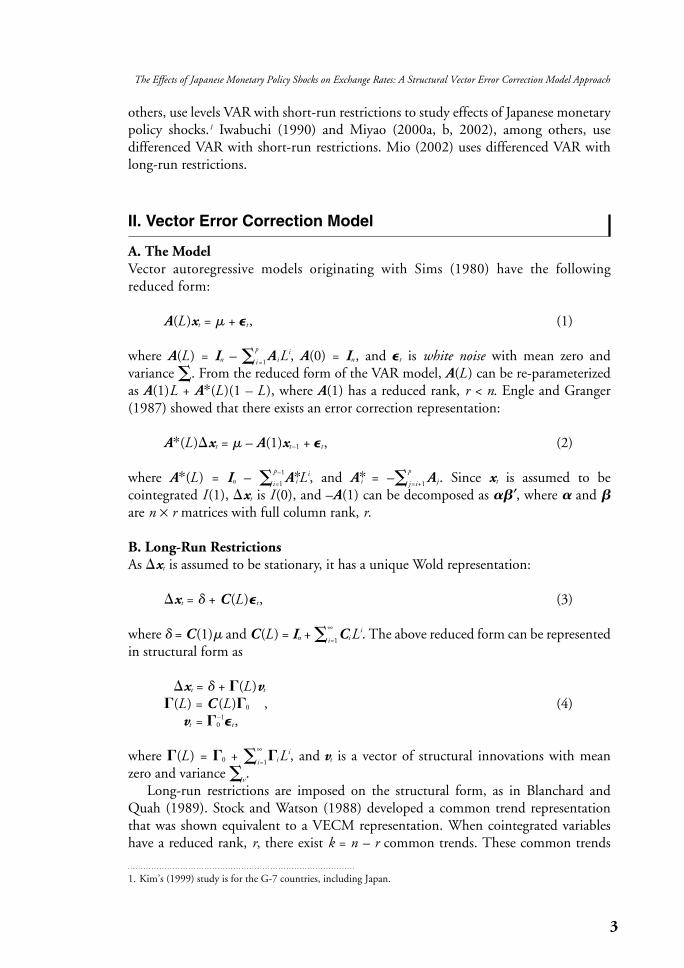
B. Long-Run RestrictionsAs �xt is assumed to be stationary, it has a unique Wold representation:

�xt = � + C (L )�t , (3)

where � = C (1)� and C (L ) = In + �∞

i=1CiLi. The above reduced form can be represented

in structural form as

�xt = � + �(L )vt

�(L ) = C (L )�0 , (4)vt = �0

–1�t ,

where �(L ) = �0 + �∞

i=1�iLi, and vt is a vector of structural innovations with mean

zero and variance �v.Long-run restrictions are imposed on the structural form, as in Blanchard and

Quah (1989). Stock and Watson (1988) developed a common trend representationthat was shown equivalent to a VECM representation. When cointegrated variableshave a reduced rank, r, there exist k = n – r common trends. These common trends

3

The Effects of Japanese Monetary Policy Shocks on Exchange Rates: A Structural Vector Error Correction Model Approach

1. Kim’s (1999) study is for the G-7 countries, including Japan.

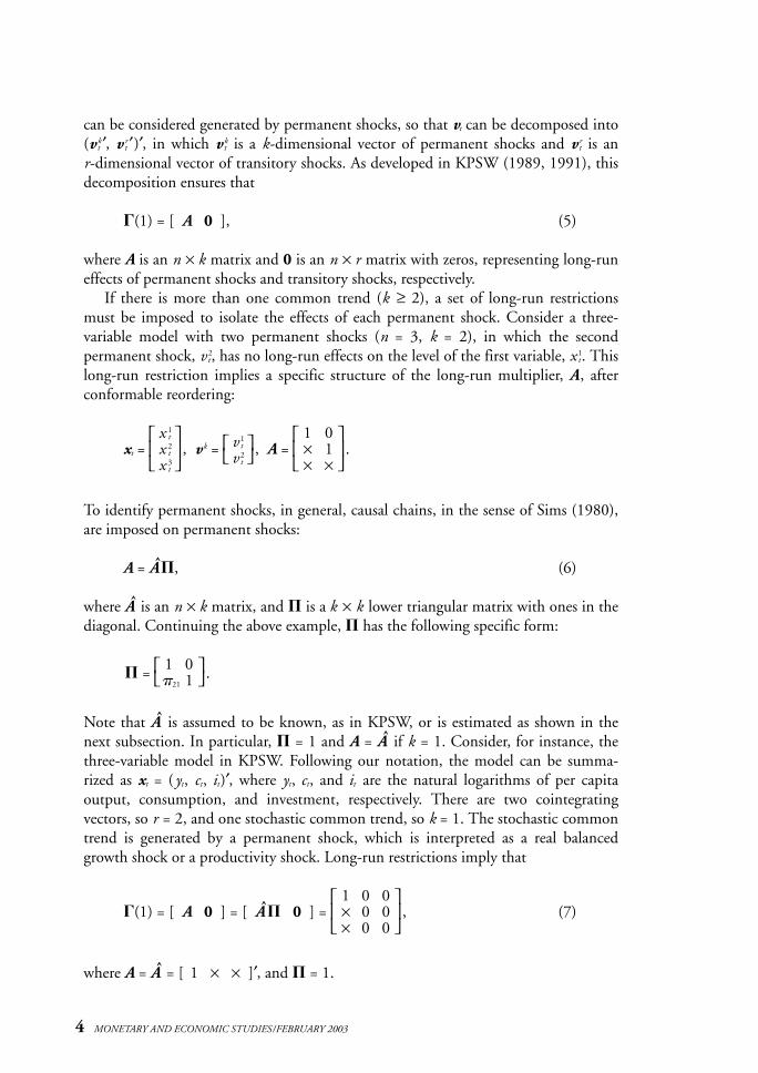
can be considered generated by permanent shocks, so that vt can be decomposed into(v t

k ′, v tr ′)′, in which v t

k is a k-dimensional vector of permanent shocks and v tr is an

r-dimensional vector of transitory shocks. As developed in KPSW (1989, 1991), thisdecomposition ensures that

�(1) = [ A 0 ], (5)

where A is an n × k matrix and 0 is an n × r matrix with zeros, representing long-runeffects of permanent shocks and transitory shocks, respectively.

If there is more than one common trend (k ≥ 2), a set of long-run restrictionsmust be imposed to isolate the effects of each permanent shock. Consider a three-variable model with two permanent shocks (n = 3, k = 2), in which the second permanent shock, v 2

t, has no long-run effects on the level of the first variable, x 1t. This

long-run restriction implies a specific structure of the long-run multiplier, A, afterconformable reordering:

x 1t v 1

t 1 0 xt = x 2

t , v k = v 2t , A = × 1 .

x 3t × ×

To identify permanent shocks, in general, causal chains, in the sense of Sims (1980),are imposed on permanent shocks:

A = A�, (6)

where A is an n × k matrix, and � is a k × k lower triangular matrix with ones in thediagonal. Continuing the above example, � has the following specific form:

� = 1 0 .�21 1

Note that A is assumed to be known, as in KPSW, or is estimated as shown in thenext subsection. In particular, � = 1 and A = A if k = 1. Consider, for instance, thethree-variable model in KPSW. Following our notation, the model can be summa-rized as xt = (yt, ct, it)′, where yt, ct, and it are the natural logarithms of per capita output, consumption, and investment, respectively. There are two cointegrating vectors, so r = 2, and one stochastic common trend, so k = 1. The stochastic commontrend is generated by a permanent shock, which is interpreted as a real balancedgrowth shock or a productivity shock. Long-run restrictions imply that

1 0 0 �(1) = [ A 0 ] = [ A � 0 ] = × 0 0 , (7)

× 0 0

where A = A = [ 1 × × ]′, and � = 1.


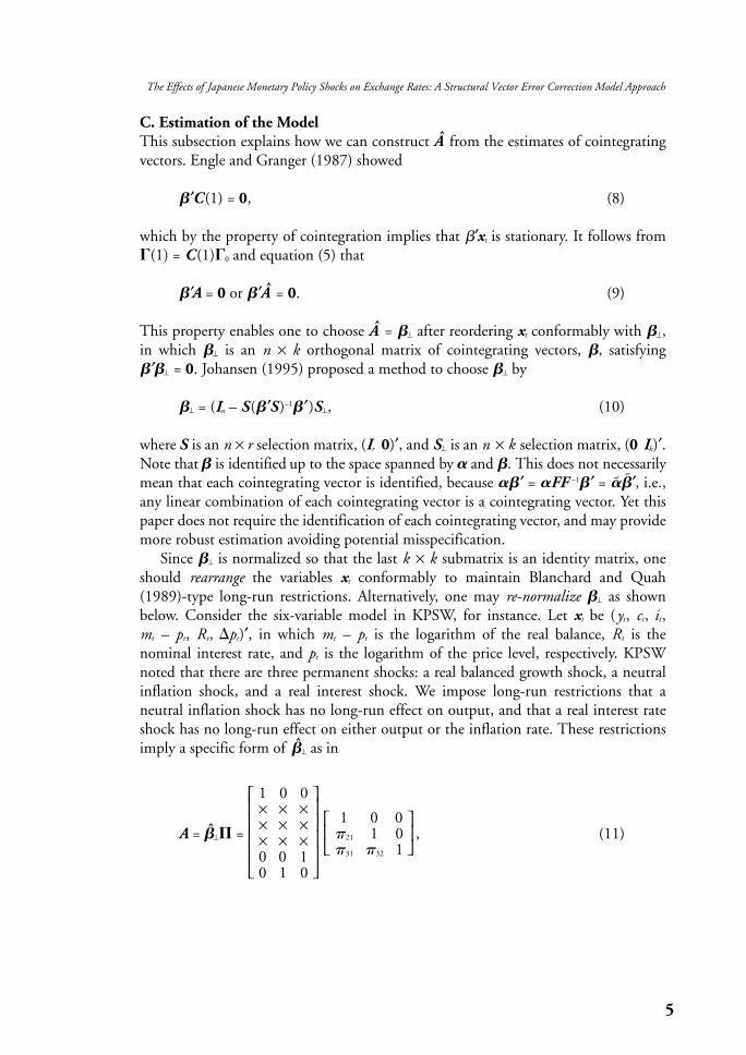
C. Estimation of the ModelThis subsection explains how we can construct A from the estimates of cointegratingvectors. Engle and Granger (1987) showed

�′C (1) = 0, (8)

which by the property of cointegration implies that �′xt is stationary. It follows from�(1) = C (1)�0 and equation (5) that

�′A = 0 or �′A = 0. (9)

This property enables one to choose A = �⊥ after reordering xt conformably with �⊥,in which �⊥ is an n × k orthogonal matrix of cointegrating vectors, �, satisfying �′�⊥ = 0. Johansen (1995) proposed a method to choose �⊥ by

�⊥ = (In – S(�′S )–1�′)S⊥, (10)

where S is an n × r selection matrix, (Ir 0)′, and S⊥ is an n × k selection matrix, (0 Ik)′.Note that � is identified up to the space spanned by � and �. This does not necessarilymean that each cointegrating vector is identified, because ��′ = �FF –1�′ = ��′, i.e.,any linear combination of each cointegrating vector is a cointegrating vector. Yet thispaper does not require the identification of each cointegrating vector, and may providemore robust estimation avoiding potential misspecification.

Since �⊥ is normalized so that the last k × k submatrix is an identity matrix, oneshould rearrange the variables xt conformably to maintain Blanchard and Quah(1989)-type long-run restrictions. Alternatively, one may re-normalize �⊥ as shownbelow. Consider the six-variable model in KPSW, for instance. Let xt be (yt, ct, it ,mt – pt, Rt, �pt)′, in which mt – pt is the logarithm of the real balance, Rt is the nominal interest rate, and pt is the logarithm of the price level, respectively. KPSWnoted that there are three permanent shocks: a real balanced growth shock, a neutralinflation shock, and a real interest shock. We impose long-run restrictions that a neutral inflation shock has no long-run effect on output, and that a real interest rateshock has no long-run effect on either output or the inflation rate. These restrictionsimply a specific form of �⊥ as in

1 0 0 × × ×

1 0 0 A = �⊥� = × × × �21 1 0 , (11) × × × �31 �32 1 0 0 1

0 1 0

5


where × denotes that those parameters are not restricted other than �′�⊥ = 0. From A = A�, we can choose A using2

A = �⊥. (12)

D. Identification of Permanent ShocksIs it possible to derive structural parameters from reduced-form estimates? This is a general identification problem that arises in most economic models. The identification problem in this paper is how structural parameters (�(L)) and the structural shock (vt) can be derived from parameters (C (L)) and residuals (�t) estimated from the reduced form. From equation (4), all structural parameters andstructural shocks can be derived from the estimates of the reduced form in equation(2) once �0 is identified.

In the framework of traditional VAR models, Sims (1980)-type causal chainrestrictions are imposed, and �0 is assumed to be a lower triangular matrix. It isdebatable, however, whether the causal chain that is assumed to identify innovationsin traditional VAR models is appropriate. As a result, VAR models have evolved tostructural VAR models with various restrictions. Contemporaneous short-run restric-tions are used in Blanchard and Watson (1986), Bernanke (1986), and Blanchard(1989), while long-run restrictions are used in Blanchard and Quah (1989).

It is worth noting that Sims (1980)-type causal chain restrictions cannot bedirectly applied to VECMs, as �0 cannot simply be assumed to be a lower triangularmatrix due to the presence of cointegration.3 This paper imposes long-run restrictionson structural shocks. These additional assumptions not only provide sufficient conditions to identify structural shocks, but also enable investigation of impulseresponse analysis in a Johansen (1988)-type VECM.

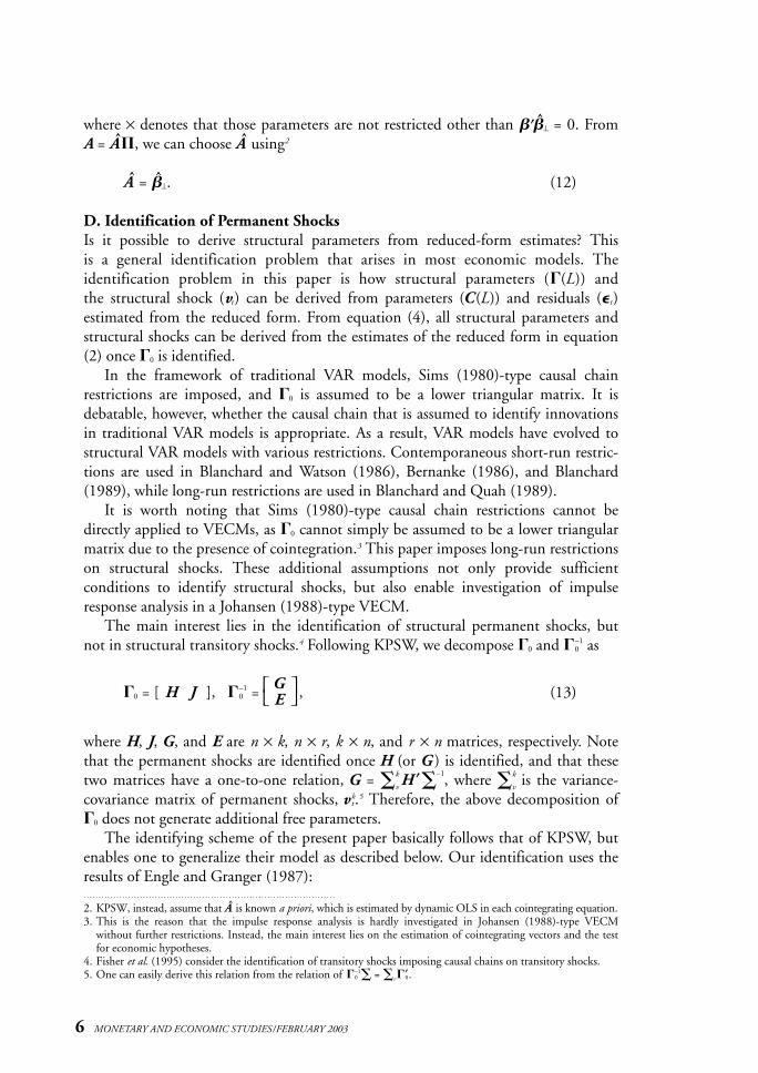
The main interest lies in the identification of structural permanent shocks, butnot in structural transitory shocks.4 Following KPSW, we decompose �0 and �0

–1 as

�0 = [ H J ], �0–1 = G , (13) E

where H, J, G, and E are n × k, n × r, k × n, and r × n matrices, respectively. Notethat the permanent shocks are identified once H (or G ) is identified, and that thesetwo matrices have a one-to-one relation, G = �

k

v H ′�–1, where �

k

v is the variance-covariance matrix of permanent shocks, v k

t .5 Therefore, the above decomposition of�0 does not generate additional free parameters.

The identifying scheme of the present paper basically follows that of KPSW, butenables one to generalize their model as described below. Our identification uses theresults of Engle and Granger (1987):


2. KPSW, instead, assume that A is known a priori, which is estimated by dynamic OLS in each cointegrating equation.3. This is the reason that the impulse response analysis is hardly investigated in Johansen (1988)-type VECM

without further restrictions. Instead, the main interest lies on the estimation of cointegrating vectors and the testfor economic hypotheses.

4. Fisher et al. (1995) consider the identification of transitory shocks imposing causal chains on transitory shocks.5. One can easily derive this relation from the relation of �0

–1� = �v�′0.

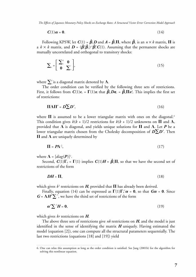
C (1)� = 0. (14)

Following KPSW, let C (1) = �⊥D and A = �⊥�, where �⊥ is an n × k matrix, � isa k × k matrix, and D = (� ′⊥�⊥)–1�′⊥C (1). Assuming that the permanent shocks aremutually uncorrelated and orthogonal to transitory shocks:

�k

v 0 �v = , (15)

0 �r

v

where �k

v is a diagonal matrix denoted by �.The order condition can be verified by the following three sets of restrictions.

First, it follows from C (1)�t = �(1)vt that �⊥D�t = �⊥�v kt. This implies the first set

of restrictions:

��′ = D�D ′, (16)

where � is assumed to be a lower triangular matrix with ones on the diagonal.6

This condition gives k (k + 1)/2 restrictions for k (k + 1)/2 unknowns on � and �,provided that � is diagonal, and yields unique solutions for � and �. Let P be alower triangular matrix chosen from the Cholesky decomposition of D�D ′. Then� and � are uniquely determined by

� = P�–1–2, (17)

where � = [diag (P )]2.Second, C (1)�0 = �(1) implies C (1)H = �⊥�, so that we have the second set of

restrictions of the form

DH = �, (18)

which gives k 2 restrictions on H, provided that � has already been derived.Finally, equation (14) can be expressed as �(1)�0

–1� = 0, so that G� = 0. Since G = �H ′�

–1, we have the third set of restrictions of the form

�′�–1H = 0, (19)

which gives kr restrictions on H.The above three sets of restrictions give nk restrictions on H, and the model is just

identified in the sense of identifying the matrix H uniquely. Having estimated themodel (equation [2]), one can compute all the structural parameters sequentially. Thelast two restrictions (equations [18] and [19]) yield

7


6. One can relax this assumption as long as the order condition is satisfied. See Jang (2001b) for the algorithm forsolving this nonlinear equation.

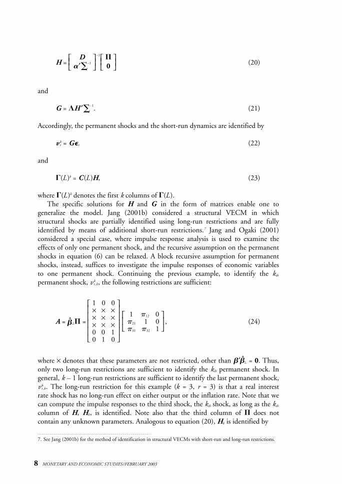
D –1 � H = (20) �′�

–1

0

and

G = �H ′�–1. (21)

Accordingly, the permanent shocks and the short-run dynamics are identified by

v kt = G�t (22)

and

�(L )k = C (L )H, (23)

where �(L )k denotes the first k columns of �(L ).The specific solutions for H and G in the form of matrices enable one to

generalize the model. Jang (2001b) considered a structural VECM in which structural shocks are partially identified using long-run restrictions and are fully identified by means of additional short-run restrictions.7 Jang and Ogaki (2001) considered a special case, where impulse response analysis is used to examine theeffects of only one permanent shock, and the recursive assumption on the permanentshocks in equation (6) can be relaxed. A block recursive assumption for permanentshocks, instead, suffices to investigate the impulse responses of economic variables to one permanent shock. Continuing the previous example, to identify the kth

permanent shock, vkt ,k, the following restrictions are sufficient:

1 0 0 × × ×

1 �12 0 A = �⊥� = × × × �21 1 0 , (24) × × × �31 �32 1 0 0 1

0 1 0

where × denotes that these parameters are not restricted, other than �′�⊥ = 0. Thus,only two long-run restrictions are sufficient to identify the kth permanent shock. Ingeneral, k – 1 long-run restrictions are sufficient to identify the last permanent shock,vk

t ,k. The long-run restriction for this example (k = 3, r = 3) is that a real interest rate shock has no long-run effect on either output or the inflation rate. Note that wecan compute the impulse responses to the third shock, the kth shock, as long as the kth

column of H, Hk, is identified. Note also that the third column of � does not contain any unknown parameters. Analogous to equation (20), Hk is identified by


7. See Jang (2001b) for the method of identification in structural VECMs with short-run and long-run restrictions.

D –1

Hk = Sk , (25) �′�

–1

where Sk is an n-dimensional selection vector with one at the kth row and zeros atother rows, (0, 0, 1, 0, 0, 0)′ for this example. Similarly, Gk is identified by

Gk = �k,kHk′�–1, (26)

and it follows from the identity relation of GH = Ik that

�k,k = (Hk′�–1Hk)–1, (27)

where �k,k is the variance of the kth permanent shock. Thus, the kth permanent shockis identified by

v kt ,k = Gk �t . (28)

III. Impulse Response Analysis with Long-Run Restrictions

This section investigates the effects of contractionary shock to the monetary policy oneconomic variables including output, price, and the yen/dollar exchange rate. Monthlyobservations from January 1975 to December 1993 are used in our empirical analysis.We end the sample period in December 1993 because the Bank of Japan’s low interestrate policy starting around this period is likely to cause a structural break (see, e.g.,Miyao [2000b]). The seven-variable model includes the call rate (rjp), a measure ofmonetary aggregate, output in Japan (yjp), price in Japan (Pjp), output in the UnitedStates (yus), the federal funds rate in the United States (rus), and the real exchange rate(er, yen/dollar). The call rate is taken from the International Financial Statistics (IFS)database, line 60b. Output in Japan is measured by industrial production, line 66c.The consumer price index is used as the price. The federal funds rate is from theFederal Reserve database. The yen/dollar exchange rate is obtained from the FederalReserve database. The real exchange rate is calculated from the nominal exchange rate and consumer price indexes. Seven alternative measures of monetary aggregate areused as described below. None of the data series is seasonally adjusted. Therefore, weinclude seasonal dummies in the VECM and VAR. We select 11 lags as the lag lengthof structural VECM, which is equivalent to 12 lags in levels VAR.

Jang and Ogaki (2001) apply Jang’s (2001a) method to U.S. data to study effectsof U.S. monetary policy shocks on economic variables. They follow Eichenbaum andEvans (1995) and use the non-borrowed reserve ratio (the ratio of non-borrowedreserves to total reserves) as the measure of monetary aggregate. They show that long-run restrictions lead to estimates of impulse responses that are roughly consis-tent with standard exchange rate models. For U.S. monetary policy, open market operations play a very important role, and non-borrowed reserves are considered tobe an appropriate measure of the monetary aggregate for the purpose of studying

9


monetary policy. This is in contrast with Japanese monetary policy, for which openmarket operations have not been important. For this reason, we report results for alternative measures of monetary aggregates.

For measures of monetary aggregates, M1, M2, M2+CDs, monetary base, thenon-borrowed reserve ratio, total reserves, and borrowed reserves are used. Monthlyaverage data for total reserves, monetary base, M1, M2, and M2+CDs were obtainedfrom the Bank of Japan homepage. Borrowed reserves are measured as “lendings frommonetary authorities” taken from the end-of-period data in the Bank of Japan’sMonetary Survey. The non-borrowed reserve ratio is calculated from end-of-perioddata for total and borrowed reserves in the Bank of Japan’s Monetary Survey by firsttaking the difference between total reserves and borrowed reserves and then dividingthe difference by total reserves.

As mentioned above, the non-borrowed reserve ratio is not a natural measure ofmonetary aggregates for studying monetary policy in Japan. This variable is includedin our study for the purpose of comparing the results in this paper with those forU.S. monetary policy in the papers cited above. Borrowed reserves are included inour study because of their potential importance in Bank of Japan loans to banks (see,e.g., Shioji [2000]). However, it should be noted that the end-of-period data are usedfor these two variables.

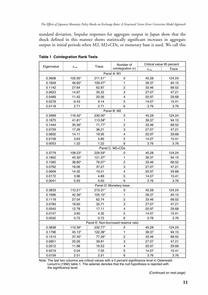
Table 1 summarizes Johansen’s (1988) cointegration rank tests over the sampleperiod January 1975–December 1993. The maximum eigenvalue tests and trace testssuggest r = 2 for M1 and monetary base, r = 3 for M2, M2+CDs, the non-borrowedreserve ratio, and total reserves, and r = 4 for borrowed reserves as the number of cointegrating vectors with a 5 percent significance level.8 Given these mixed results, we choose r by conjecturing the number of permanent shocks in the model.The permanent shocks include a Japanese supply shock and a U.S. supply shock. The permanent shocks also include a shock that affects the long-run level of real exchange rates (a real exchange rate shock) and a Japanese monetary policy shock thataffects the long-run level of Japanese prices. A U.S. monetary policy shock can beconsidered as a transitory shock, since the model does not include the U.S. prices,while it can be considered as a permanent shock if it affects the long-run level of U.S. interest rates. Therefore, we report the results with four permanent shocks (k = 4, r = 3) in a benchmark model, and we check the robustness of the results usingk = 5 and r = 2. In a benchmark model, the Japanese monetary shock is identified bythree long-run restrictions: the shock does not affect Japanese output, U.S. output,and real exchange rates in the long run. Our main results do not change when weadopt k = 5 with an additional assumption that the Japanese monetary shock doesnot affect the U.S. interest rates in the long run.9

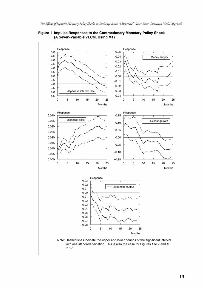
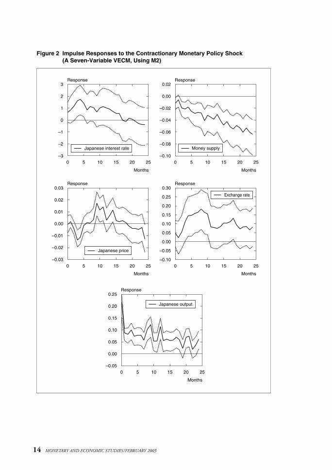
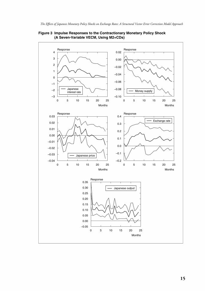
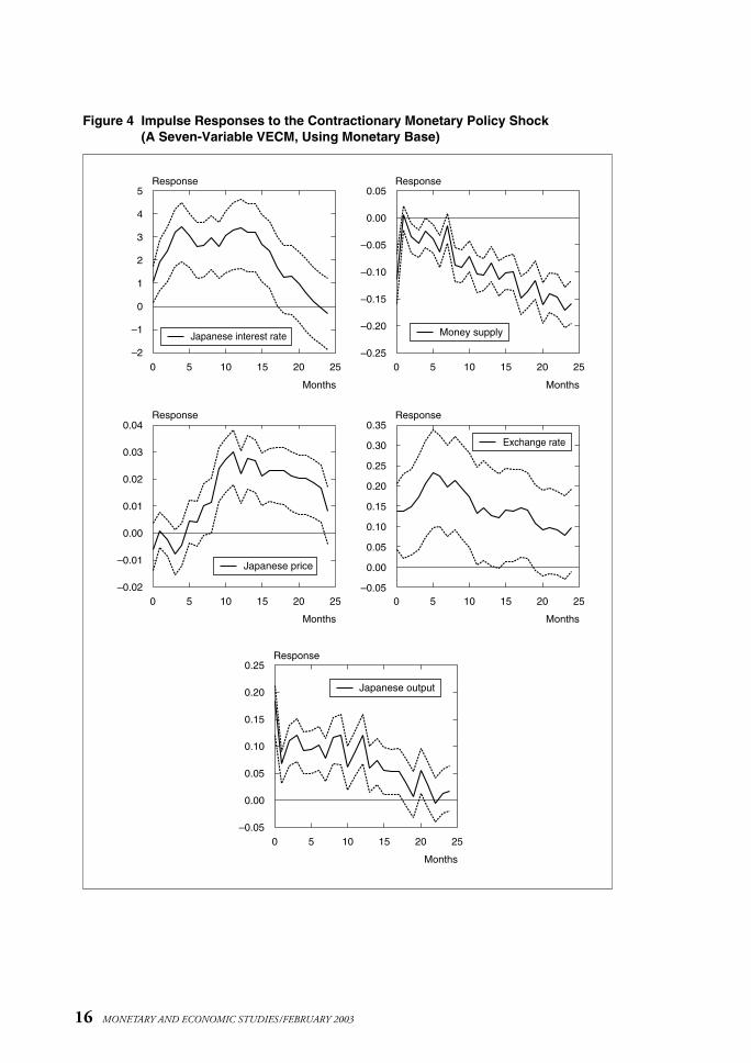
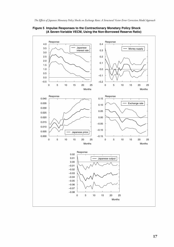
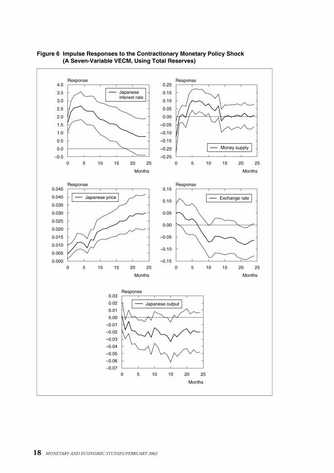
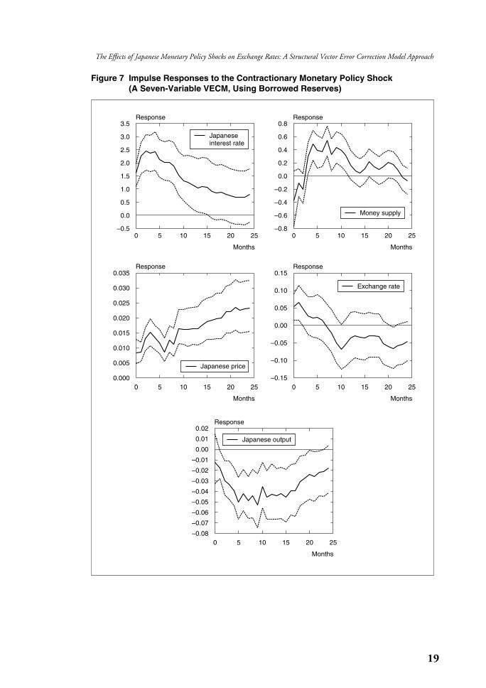
Results for M1, M2, M2+CDs, monetary base, the non-borrowed reserve ratio,total reserves, and borrowed reserves are reported in Figures 1 to 7. In these figures, acontractionary monetary shock is defined as a shock that initially increases the call rate. Significance intervals are drawn by Monte Carlo integration with one


8. We select the model that satisfies the deterministic cointegration restriction developed in Ogaki and Park (1997).9. The results are available upon request.

11


standard deviation. Impulse responses for aggregate output in Japan show that theshock defined in this manner shows statistically significant increases in aggregate output in initial periods when M2, M2+CDs, or monetary base is used. We call this

Table 1 Cointegration Rank Tests

Eigenvalue max Trace Number of Critical value 95 percentcointegration (r ) max Trace

Panel A: M10.3608 102.05* 211.51* 0 45.28 124.240.1849 46.60* 109.47* 1 39.37 94.150.1142 27.64 62.87 2 33.46 68.520.0623 14.67 35.22 3 27.07 47.210.0489 11.42 20.56 4 20.97 29.680.0278 6.43 9.14 5 14.07 15.410.0118 2.71 2.71 6 3.76 3.76

Panel B: M20.3999 116.42* 230.00* 0 45.28 124.240.1675 41.81* 113.58* 1 39.37 94.150.1444 35.56* 71.77* 2 33.46 68.520.0729 17.26 36.21 3 27.07 47.210.0600 14.11 18.95 4 20.97 29.680.0158 3.63 4.85 5 14.07 15.410.0053 1.22 1.22 6 3.76 3.76

Panel C: M2+CDs0.3779 108.23* 229.59* 0 45.28 124.240.1802 45.30* 121.37* 1 39.37 94.150.1565 38.80* 76.07* 2 33.46 68.520.0762 18.06 37.27 3 27.07 47.210.0609 14.32 19.21 4 20.97 29.680.0172 3.96 4.89 5 14.07 15.410.0041 0.93 0.93 6 3.76 3.76

Panel D: Monetary base0.3833 110.21* 215.31* 0 45.28 124.240.1696 42.36* 105.10* 1 39.37 94.150.1118 27.04 62.74 2 33.46 68.520.0783 18.60 35.71 3 27.07 47.210.0545 12.78 17.11 4 20.97 29.680.0157 3.60 4.32 5 14.07 15.410.0032 0.72 0.72 6 3.76 3.76

Panel E: Non-borrowed reserve ratio0.3838 110.39* 232.77* 0 45.28 124.240.1796 45.13* 122.38* 1 39.37 94.150.1515 37.45* 77.26* 2 33.46 68.520.0851 20.26 39.81 3 27.07 47.210.0512 11.98 19.53 4 20.97 29.680.0219 5.04 7.55 5 14.07 15.410.0109 2.51 2.51 6 3.76 3.76

Note: The last two columns are critical values with a 5 percent significance level in Osterwald-Lenum’s (1992) table 1. The asterisk denotes that the null hypothesis is rejected with the significance level.

(Continued on next page)


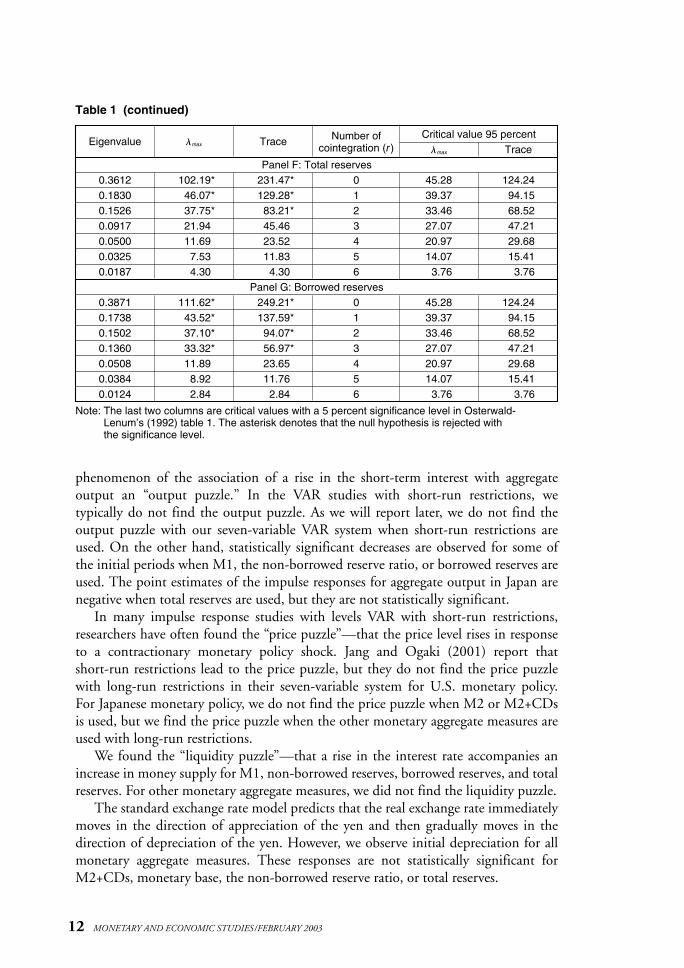
Table 1 (continued)

Eigenvalue max Trace Number of Critical value 95 percentcointegration (r ) max Trace

Panel F: Total reserves0.3612 102.19* 231.47* 0 45.28 124.240.1830 46.07* 129.28* 1 39.37 94.150.1526 37.75* 83.21* 2 33.46 68.520.0917 21.94 45.46 3 27.07 47.210.0500 11.69 23.52 4 20.97 29.680.0325 7.53 11.83 5 14.07 15.410.0187 4.30 4.30 6 3.76 3.76

Panel G: Borrowed reserves0.3871 111.62* 249.21* 0 45.28 124.240.1738 43.52* 137.59* 1 39.37 94.150.1502 37.10* 94.07* 2 33.46 68.520.1360 33.32* 56.97* 3 27.07 47.210.0508 11.89 23.65 4 20.97 29.680.0384 8.92 11.76 5 14.07 15.410.0124 2.84 2.84 6 3.76 3.76

Note: The last two columns are critical values with a 5 percent significance level in Osterwald-Lenum’s (1992) table 1. The asterisk denotes that the null hypothesis is rejected with the significance level.

phenomenon of the association of a rise in the short-term interest with aggregate output an “output puzzle.” In the VAR studies with short-run restrictions, we typically do not find the output puzzle. As we will report later, we do not find theoutput puzzle with our seven-variable VAR system when short-run restrictions areused. On the other hand, statistically significant decreases are observed for some ofthe initial periods when M1, the non-borrowed reserve ratio, or borrowed reserves areused. The point estimates of the impulse responses for aggregate output in Japan arenegative when total reserves are used, but they are not statistically significant.

In many impulse response studies with levels VAR with short-run restrictions,researchers have often found the “price puzzle”—that the price level rises in responseto a contractionary monetary policy shock. Jang and Ogaki (2001) report that short-run restrictions lead to the price puzzle, but they do not find the price puzzlewith long-run restrictions in their seven-variable system for U.S. monetary policy.For Japanese monetary policy, we do not find the price puzzle when M2 or M2+CDsis used, but we find the price puzzle when the other monetary aggregate measures areused with long-run restrictions.

We found the “liquidity puzzle”—that a rise in the interest rate accompanies anincrease in money supply for M1, non-borrowed reserves, borrowed reserves, and totalreserves. For other monetary aggregate measures, we did not find the liquidity puzzle.

The standard exchange rate model predicts that the real exchange rate immediatelymoves in the direction of appreciation of the yen and then gradually moves in thedirection of depreciation of the yen. However, we observe initial depreciation for allmonetary aggregate measures. These responses are not statistically significant forM2+CDs, monetary base, the non-borrowed reserve ratio, or total reserves.

13


Figure 1 Impulse Responses to the Contractionary Monetary Policy Shock (A Seven-Variable VECM, Using M1)

4.03.53.02.52.01.51.00.50.0

–0.5–1.0–1.5

0.05

0.04

0.03

0.02

0.01

0.00

–0.01

–0.02

–0.03

–0.04

0.040

0.035

0.030

0.025

0.020

0.015

0.010

0.005

0.000

0.030.020.010.00

–0.01–0.02–0.03–0.04–0.05–0.06–0.07–0.08

0.15

0.10

0.05

0.00

–0.05

–0.10

–0.15

0 5 10 15 20 25

Months

0 5 10 15 20 25

Months

0 5 10 15 20 25

Months

0 5 10 15 20 25

Months

0 5 10 15 20 25

Months

Response Response

Response

Response

Response

Japanese interest rate

Japanese output

Japanese price

Money supply

Exchange rate

Note: Dashed lines indicate the upper and lower bounds of the significant intervalwith one standard deviation. This is also the case for Figures 1 to 7 and 13to 17.


Figure 2 Impulse Responses to the Contractionary Monetary Policy Shock (A Seven-Variable VECM, Using M2)

3

2

1

0

–1

–2

–3

0.02

0.00

–0.02

–0.04

–0.06

–0.08

–0.10

0.03

0.02

0.01

0.00

–0.01

–0.02

–0.03

0.25

0.20

0.15

0.10

0.05

0.00

–0.05

0.30

0.25

0.20

0.15

0.10

0.05

0.00

–0.05

–0.10

0 5 10 15 20 25

Months

0 5 10 15 20 25

Months

0 5 10 15 20 25

Months

0 5 10 15 20 25

Months

0 5 10 15 20 25

Months

Response Response

Response

Response

Response


Japanese output

Japanese price

Money supply

Exchange rate

15


Figure 3 Impulse Responses to the Contractionary Monetary Policy Shock (A Seven-Variable VECM, Using M2+CDs)

4

3

2

1

0

–1

–2

–3

0.02

0.00

–0.02

–0.04

–0.06

–0.08

–0.10

0.03

0.02

0.01

0.00

–0.01

–0.02

–0.03

–0.04

0.35

0.30

0.25

0.20

0.15

0.10

0.05

0.00

–0.05

0.4

0.3

0.2

0.1

0.0

–0.1

–0.2

0 5 10 15 20 25

Months

0 5 10 15 20 25

Months

0 5 10 15 20 25

Months

0 5 10 15 20 25

Months

0 5 10 15 20 25

Months

Response Response

Response

Response

Response


Japanese output

Japanese price

Money supply

Exchange rate


Figure 4 Impulse Responses to the Contractionary Monetary Policy Shock (A Seven-Variable VECM, Using Monetary Base)

5

4

3

2

1

0

–1

–2

0.05

0.00

–0.05

–0.10

–0.15

–0.20

–0.25

0.04

0.03

0.02

0.01

0.00

–0.01

–0.02

0.25

0.20

0.15

0.10

0.05

0.00

–0.05

0.35

0.30

0.25

0.20

0.15

0.10

0.05

0.00

–0.05

0 5 10 15 20 25

Months

0 5 10 15 20 25

Months

0 5 10 15 20 25

Months

0 5 10 15 20 25

Months

0 5 10 15 20 25

Months

Response Response

Response

Response

Response


Japanese output

Japanese price

Money supply

Exchange rate

17


Figure 5 Impulse Responses to the Contractionary Monetary Policy Shock (A Seven-Variable VECM, Using the Non-Borrowed Reserve Ratio)

4.0

3.5

3.0

2.5

2.0

1.5

1.0

0.5

0.0

–0.5

0.4

0.3

0.2

0.1

0.0

–0.1

–0.2

0.040

0.035

0.030

0.025

0.020

0.015

0.010

0.005

0.000

0.02

0.01

0.00

–0.01

–0.02

–0.03

–0.04

–0.05

–0.06

–0.07

–0.08

0.15

0.10

0.05

0.00

–0.05

–0.10

–0.15

0 5 10 15 20 25

Months

0 5 10 15 20 25

Months

0 5 10 15 20 25

Months

0 5 10 15 20 25

Months

0 5 10 15 20 25

Months

Response Response

Response

Response

Response

Japanese output

Japanese price

Money supply

Exchange rate



Figure 6 Impulse Responses to the Contractionary Monetary Policy Shock (A Seven-Variable VECM, Using Total Reserves)

4.0

3.5

3.0

2.5

2.0

1.5

1.0

0.5

0.0

–0.5

0.20

0.15

0.10

0.05

0.00

–0.05

–0.10

–0.15

–0.20

–0.25

0.045

0.040

0.035

0.030

0.025

0.020

0.015

0.010

0.005

0.000

0.03

0.02

0.01

0.00

–0.01

–0.02

–0.03

–0.04

–0.05

–0.06

–0.07

0.15

0.10

0.05

0.00

–0.05

–0.10

–0.15

0 5 10 15 20 25

Months

0 5 10 15 20 25

Months

0 5 10 15 20 25

Months

0 5 10 15 20 25

Months

0 5 10 15 20 25

Months

Response Response

Response

Response

Response

Japanese output

Japanese price

Money supply

Exchange rate


19


Figure 7 Impulse Responses to the Contractionary Monetary Policy Shock (A Seven-Variable VECM, Using Borrowed Reserves)

3.5

3.0

2.5

2.0

1.5

1.0

0.5

0.0

–0.5

0.8

0.6

0.4

0.2

0.0

–0.2

–0.4

–0.6

–0.8

0.035

0.030

0.025

0.020

0.015

0.010

0.005

0.000

0.02

0.01

0.00

–0.01

–0.02

–0.03

–0.04

–0.05

–0.06

–0.07

–0.08

0.15

0.10

0.05

0.00

–0.05

–0.10

–0.15

0 5 10 15 20 25

Months

0 5 10 15 20 25

Months

0 5 10 15 20 25

Months

0 5 10 15 20 25

Months

0 5 10 15 20 25

Months

Response Response

Response

Response

Response

Japanese output

Japanese price

Money supply

Exchange rate


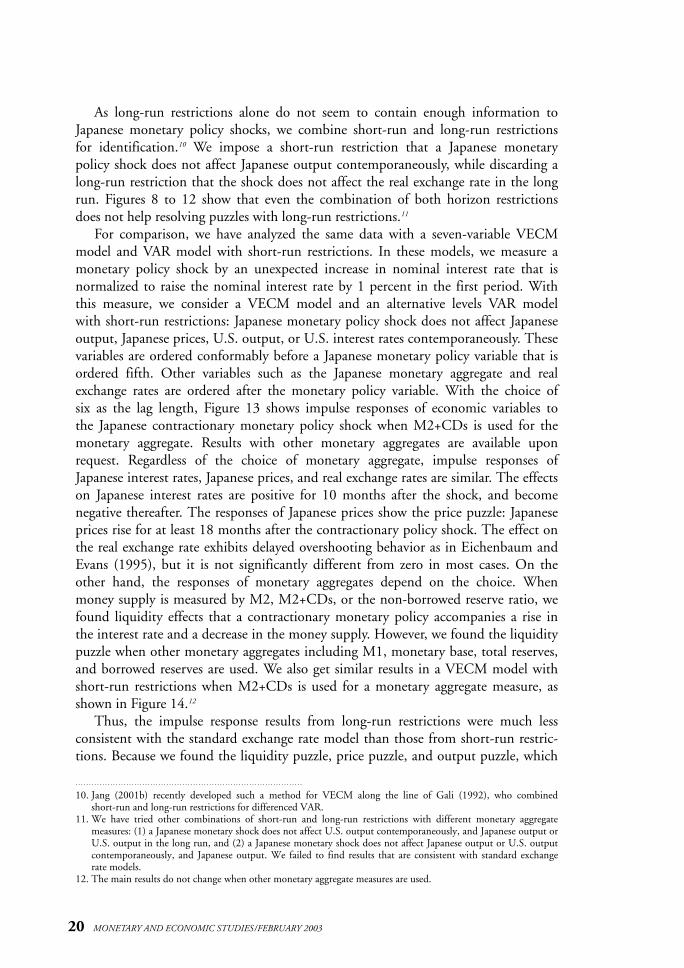
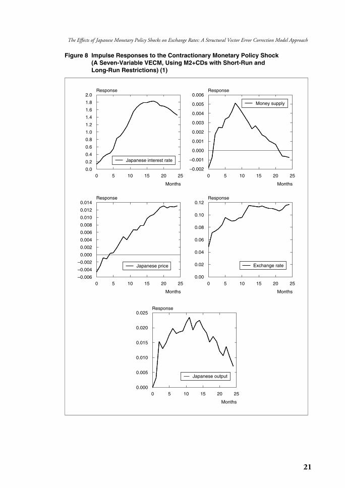
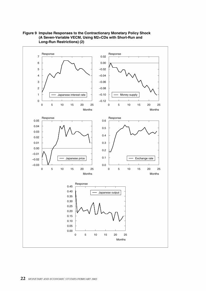
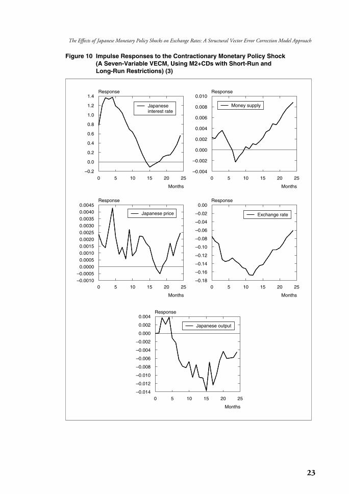
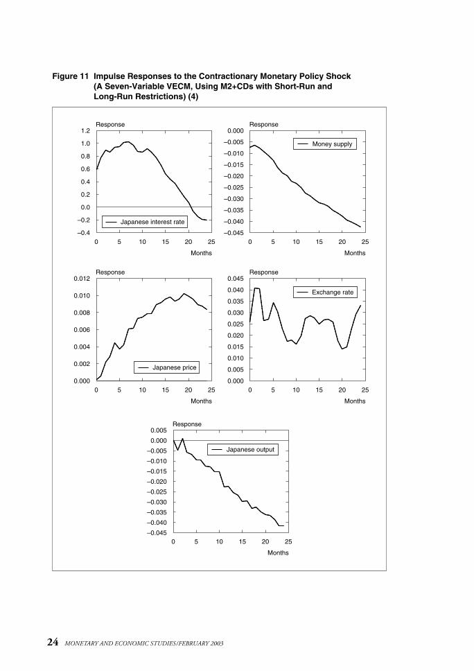
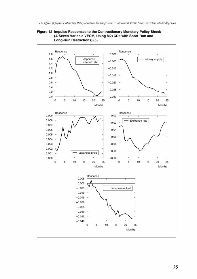
As long-run restrictions alone do not seem to contain enough information toJapanese monetary policy shocks, we combine short-run and long-run restrictions for identification.10 We impose a short-run restriction that a Japanese monetary policy shock does not affect Japanese output contemporaneously, while discarding along-run restriction that the shock does not affect the real exchange rate in the longrun. Figures 8 to 12 show that even the combination of both horizon restrictionsdoes not help resolving puzzles with long-run restrictions.11

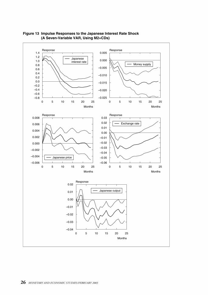
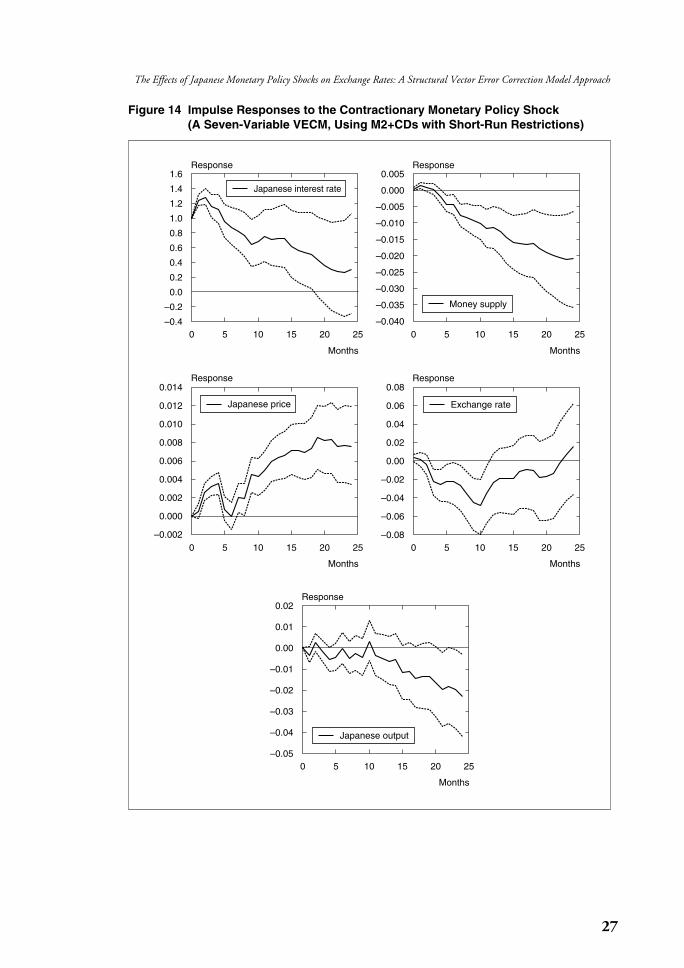
For comparison, we have analyzed the same data with a seven-variable VECMmodel and VAR model with short-run restrictions. In these models, we measure amonetary policy shock by an unexpected increase in nominal interest rate that is normalized to raise the nominal interest rate by 1 percent in the first period. Withthis measure, we consider a VECM model and an alternative levels VAR model with short-run restrictions: Japanese monetary policy shock does not affect Japaneseoutput, Japanese prices, U.S. output, or U.S. interest rates contemporaneously. Thesevariables are ordered conformably before a Japanese monetary policy variable that isordered fifth. Other variables such as the Japanese monetary aggregate and realexchange rates are ordered after the monetary policy variable. With the choice of six as the lag length, Figure 13 shows impulse responses of economic variables to the Japanese contractionary monetary policy shock when M2+CDs is used for themonetary aggregate. Results with other monetary aggregates are available uponrequest. Regardless of the choice of monetary aggregate, impulse responses ofJapanese interest rates, Japanese prices, and real exchange rates are similar. The effectson Japanese interest rates are positive for 10 months after the shock, and become negative thereafter. The responses of Japanese prices show the price puzzle: Japaneseprices rise for at least 18 months after the contractionary policy shock. The effect onthe real exchange rate exhibits delayed overshooting behavior as in Eichenbaum andEvans (1995), but it is not significantly different from zero in most cases. On theother hand, the responses of monetary aggregates depend on the choice. Whenmoney supply is measured by M2, M2+CDs, or the non-borrowed reserve ratio, wefound liquidity effects that a contractionary monetary policy accompanies a rise inthe interest rate and a decrease in the money supply. However, we found the liquiditypuzzle when other monetary aggregates including M1, monetary base, total reserves,and borrowed reserves are used. We also get similar results in a VECM model withshort-run restrictions when M2+CDs is used for a monetary aggregate measure, asshown in Figure 14.12

Thus, the impulse response results from long-run restrictions were much less consistent with the standard exchange rate model than those from short-run restric-tions. Because we found the liquidity puzzle, price puzzle, and output puzzle, which


10. Jang (2001b) recently developed such a method for VECM along the line of Gali (1992), who combined short-run and long-run restrictions for differenced VAR.

11. We have tried other combinations of short-run and long-run restrictions with different monetary aggregate measures: (1) a Japanese monetary shock does not affect U.S. output contemporaneously, and Japanese output orU.S. output in the long run, and (2) a Japanese monetary shock does not affect Japanese output or U.S. outputcontemporaneously, and Japanese output. We failed to find results that are consistent with standard exchangerate models.

12. The main results do not change when other monetary aggregate measures are used.

21


Figure 8 Impulse Responses to the Contractionary Monetary Policy Shock (A Seven-Variable VECM, Using M2+CDs with Short-Run and Long-Run Restrictions) (1)

2.0

1.8

1.6

1.4

1.2

1.0

0.8

0.6

0.4

0.2

0.0

0.006

0.005

0.004

0.003

0.002

0.001

0.000

–0.001

–0.002

0.014

0.012

0.010

0.008

0.006

0.004

0.002

0.000

–0.002

–0.004

–0.006

0.025

0.020

0.015

0.010

0.005

0.000

0.12

0.10

0.08

0.06

0.04

0.02

0.00

0 5 10 15 20 25

Months

0 5 10 15 20 25

Months

0 5 10 15 20 25

Months

0 5 10 15 20 25

Months

0 5 10 15 20 25

Months

Response Response

Response

Response

Response


Japanese output

Japanese price

Money supply

Exchange rate



7

6

5

4

3

2

1

0

0.02

0.00

–0.02

–0.04

–0.06

–0.08

–0.10

–0.12

0.05

0.04

0.03

0.02

0.01

0.00

–0.01

–0.02

–0.03

0.45

0.40

0.35

0.30

0.25

0.20

0.15

0.10

0.05

0.00

0.6

0.5

0.4

0.3

0.2

0.1

0.0

0 5 10 15 20 25

Months

0 5 10 15 20 25

Months

0 5 10 15 20 25

Months

0 5 10 15 20 25

Months

0 5 10 15 20 25

Months

Response Response

Response

Response

Response


Japanese output

Japanese price

Money supply

Exchange rate

23



1.4

1.2

1.0

0.8

0.6

0.4

0.2

0.0

–0.2

0.010

0.008

0.006

0.004

0.002

0.000

–0.002

–0.004

0.00450.00400.00350.00300.00250.00200.00150.00100.00050.0000

–0.0005–0.0010

0.004

0.002

0.000

–0.002

–0.004

–0.006

–0.008

–0.010

–0.012

–0.014

0.00

–0.02

–0.04

–0.06

–0.08

–0.10

–0.12

–0.14

–0.16

–0.18

0 5 10 15 20 25

Months

0 5 10 15 20 25

Months

0 5 10 15 20 25

Months

0 5 10 15 20 25

Months

0 5 10 15 20 25

Months

Response Response

Response

Response

Response

Japanese output

Japanese price

Money supply

Exchange rate




1.2

1.0

0.8

0.6

0.4

0.2

0.0

–0.2

–0.4

0.000

–0.005

–0.010

–0.015

–0.020

–0.025

–0.030

–0.035

–0.040

–0.045

0.012

0.010

0.008

0.006

0.004

0.002

0.000

0.005

0.000

–0.005

–0.010

–0.015

–0.020

–0.025

–0.030

–0.035

–0.040

–0.045

0.045

0.040

0.035

0.030

0.025

0.020

0.015

0.010

0.005

0.000

0 5 10 15 20 25

Months

0 5 10 15 20 25

Months

0 5 10 15 20 25

Months

0 5 10 15 20 25

Months

0 5 10 15 20 25

Months

Response Response

Response

Response

Response


Japanese output

Japanese price

Money supply

Exchange rate

25



1.8

1.6

1.4

1.2

1.0

0.8

0.6

0.4

0.2

0.0

0.000

–0.005

–0.010

–0.015

–0.020

–0.025

–0.030

0.009

0.008

0.007

0.006

0.005

0.004

0.003

0.002

0.001

0.000

0.005

0.000

–0.005

–0.010

–0.015

–0.020

–0.025

–0.030

–0.035

–0.040

0.00

–0.02

–0.04

–0.06

–0.08

–0.10

–0.12

0 5 10 15 20 25

Months

0 5 10 15 20 25

Months

0 5 10 15 20 25

Months

0 5 10 15 20 25

Months

0 5 10 15 20 25

Months

Response Response

Response

Response

Response

Japanese output

Japanese price

Money supply

Exchange rate



Figure 13 Impulse Responses to the Japanese Interest Rate Shock (A Seven-Variable VAR, Using M2+CDs)

1.41.21.00.80.60.40.20.0

–0.2–0.4–0.6–0.8

0.005

0.000

–0.005

–0.010

–0.015

–0.020

–0.025

0.008

0.006

0.004

0.002

0.000

–0.002

–0.004

–0.006

0.02

0.01

0.00

–0.01

–0.02

–0.03

–0.04

0.03

0.02

0.01

0.00

–0.01

–0.02

–0.03

–0.04

–0.05

–0.06

0 5 10 15 20 25

Months

0 5 10 15 20 25

Months

0 5 10 15 20 25

Months

0 5 10 15 20 25

Months

0 5 10 15 20 25

Months

Response Response

Response

Response

Response

Japanese output

Japanese price

Money supply

Exchange rate


27


Figure 14 Impulse Responses to the Contractionary Monetary Policy Shock (A Seven-Variable VECM, Using M2+CDs with Short-Run Restrictions)

1.6

1.4

1.2

1.0

0.8

0.6

0.4

0.2

0.0

–0.2

–0.4

0.005

0.000

–0.005

–0.010

–0.015

–0.020

–0.025

–0.030

–0.035

–0.040

0.014

0.012

0.010

0.008

0.006

0.004

0.002

0.000

–0.002

0.02

0.01

0.00

–0.01

–0.02

–0.03

–0.04

–0.05

0.08

0.06

0.04

0.02

0.00

–0.02

–0.04

–0.06

–0.08

0 5 10 15 20 25

Months

0 5 10 15 20 25

Months

0 5 10 15 20 25

Months

0 5 10 15 20 25

Months

0 5 10 15 20 25

Months

Response Response

Response

Response

Response


Japanese output

Japanese price

Money supply

Exchange rate

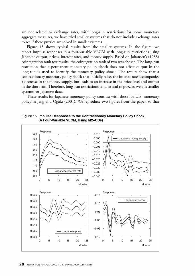
are not related to exchange rates, with long-run restrictions for some monetary aggregate measures, we have tried smaller systems that do not include exchange ratesto see if these puzzles are solved in smaller systems.

Figure 15 shows typical results from the smaller systems. In the figure, we report impulse responses in a four-variable VECM with long-run restrictions usingJapanese output, prices, interest rates, and money supply. Based on Johansen’s (1988)cointegration rank test results, the cointegration rank of two was chosen. The long-runrestriction that a permanent monetary policy shock does not affect output in the long-run is used to identify the monetary policy shock. The results show that a contractionary monetary policy shock that initially raises the interest rate accompaniesa decrease in the money supply, but leads to an increase in the price level and outputin the short run. Therefore, long-run restrictions tend to lead to puzzles even in smallersystems for Japanese data.

These results for Japanese monetary policy contrast with those for U.S. monetarypolicy in Jang and Ogaki (2001). We reproduce two figures from the paper, so that


Figure 15 Impulse Responses to the Contractionary Monetary Policy Shock (A Four-Variable VECM, Using M2+CDs)

4.0

3.5

3.0

2.5

2.0

1.5

1.0

0.5

0.0

0.010

0.005

0.000

–0.005

–0.010

–0.015

–0.020

–0.025

–0.030

–0.035

–0.040

0.035

0.030

0.025

0.020

0.015

0.010

0.005

0.000

0.15

0.10

0.05

0.00

–0.05

–0.10

0 5 10 15 20 25

Months

0 5 10 15 20 25

Months

0 5 10 15 20 25

Months

0 5 10 15 20 25

Months

Response Response

Response Response


Japanese price

Japanese money supply

Japanese output

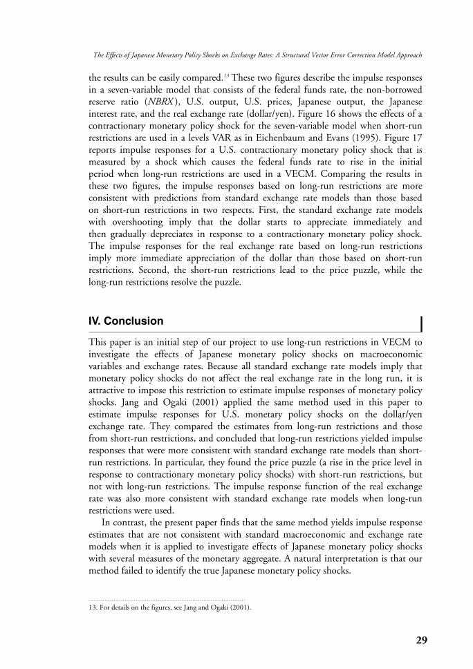
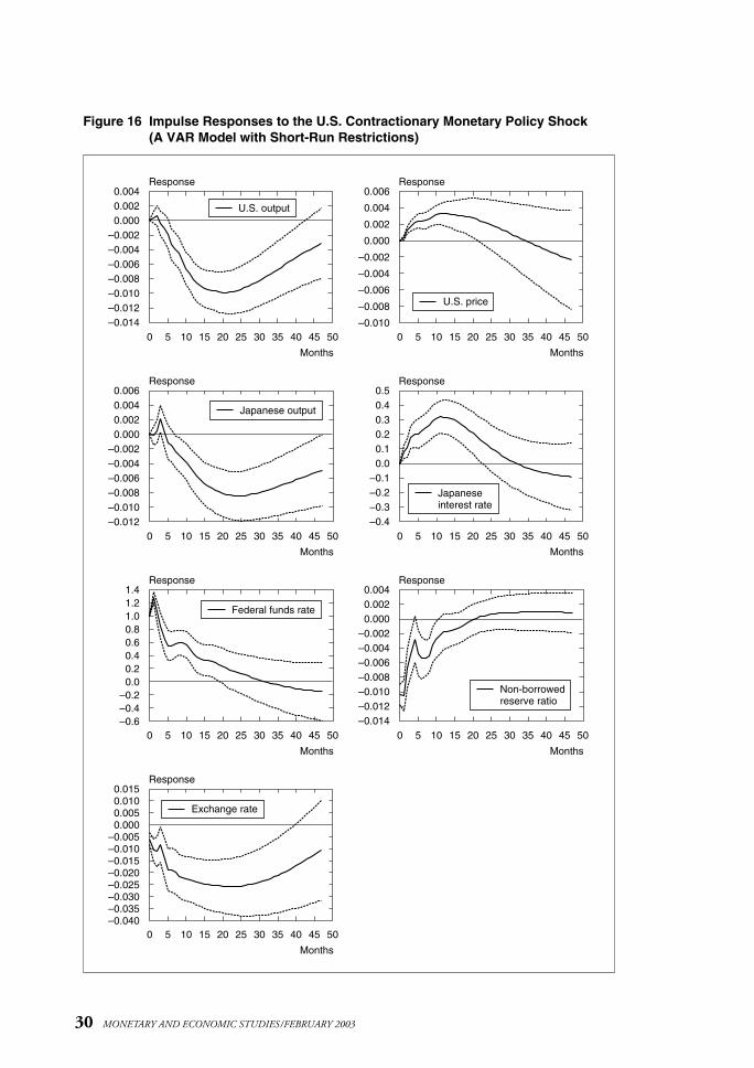
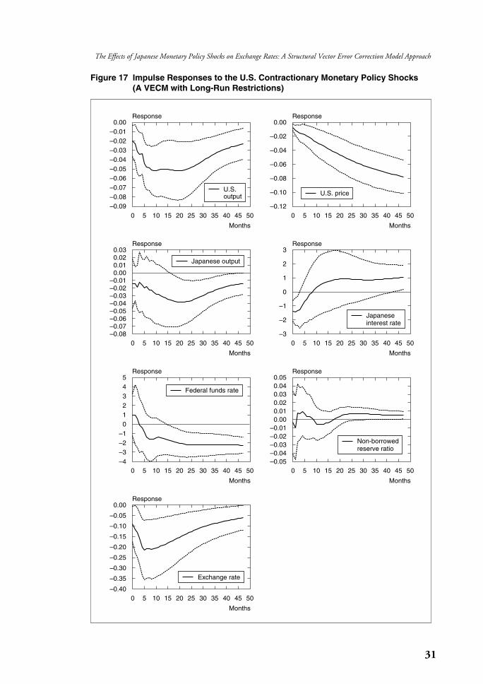
the results can be easily compared.13 These two figures describe the impulse responsesin a seven-variable model that consists of the federal funds rate, the non-borrowedreserve ratio (NBRX ), U.S. output, U.S. prices, Japanese output, the Japanese interest rate, and the real exchange rate (dollar/yen). Figure 16 shows the effects of acontractionary monetary policy shock for the seven-variable model when short-runrestrictions are used in a levels VAR as in Eichenbaum and Evans (1995). Figure 17reports impulse responses for a U.S. contractionary monetary policy shock that ismeasured by a shock which causes the federal funds rate to rise in the initial period when long-run restrictions are used in a VECM. Comparing the results inthese two figures, the impulse responses based on long-run restrictions are more consistent with predictions from standard exchange rate models than those based on short-run restrictions in two respects. First, the standard exchange rate modelswith overshooting imply that the dollar starts to appreciate immediately and then gradually depreciates in response to a contractionary monetary policy shock.The impulse responses for the real exchange rate based on long-run restrictions imply more immediate appreciation of the dollar than those based on short-runrestrictions. Second, the short-run restrictions lead to the price puzzle, while thelong-run restrictions resolve the puzzle.

IV. Conclusion

This paper is an initial step of our project to use long-run restrictions in VECM toinvestigate the effects of Japanese monetary policy shocks on macroeconomic variables and exchange rates. Because all standard exchange rate models imply thatmonetary policy shocks do not affect the real exchange rate in the long run, it isattractive to impose this restriction to estimate impulse responses of monetary policyshocks. Jang and Ogaki (2001) applied the same method used in this paper to estimate impulse responses for U.S. monetary policy shocks on the dollar/yenexchange rate. They compared the estimates from long-run restrictions and thosefrom short-run restrictions, and concluded that long-run restrictions yielded impulseresponses that were more consistent with standard exchange rate models than short-run restrictions. In particular, they found the price puzzle (a rise in the price level inresponse to contractionary monetary policy shocks) with short-run restrictions, butnot with long-run restrictions. The impulse response function of the real exchangerate was also more consistent with standard exchange rate models when long-runrestrictions were used.

In contrast, the present paper finds that the same method yields impulse responseestimates that are not consistent with standard macroeconomic and exchange ratemodels when it is applied to investigate effects of Japanese monetary policy shockswith several measures of the monetary aggregate. A natural interpretation is that ourmethod failed to identify the true Japanese monetary policy shocks.

29


13. For details on the figures, see Jang and Ogaki (2001).


Figure 16 Impulse Responses to the U.S. Contractionary Monetary Policy Shock (A VAR Model with Short-Run Restrictions)

0 5 10 15 20 25 30 35 40 45 50 0 5 10 15 20 25 30 35 40 45 50

0 5 10 15 20 25 30 35 40 45 50 0 5 10 15 20 25 30 35 40 45 50

0 5 10 15 20 25 30 35 40 45 50

0 5 10 15 20 25 30 35 40 45 50

0 5 10 15 20 25 30 35 40 45 50

0.0040.0020.000

–0.002–0.004–0.006–0.008–0.010–0.012–0.014

0.006

0.004

0.002

0.000

–0.002

–0.004

–0.006

–0.008

–0.010

Months Months

Response Response

0.0060.0040.0020.000

–0.002–0.004–0.006–0.008–0.010–0.012

0.50.40.30.20.10.0

–0.1–0.2–0.3–0.4

Months Months

Response Response

1.41.21.00.80.60.40.20.0

–0.2–0.4–0.6

0.0040.0020.000

–0.002–0.004–0.006–0.008–0.010–0.012–0.014

Months Months

Response Response

0.0150.0100.0050.000

–0.005–0.010–0.015–0.020–0.025–0.030–0.035–0.040

Months

Response

Federal funds rate

U.S. output

U.S. price

Japanese output


Non-borrowed reserve ratio

Exchange rate

31


Figure 17 Impulse Responses to the U.S. Contractionary Monetary Policy Shocks (A VECM with Long-Run Restrictions)

0 5 10 15 20 25 30 35 40 45 50 0 5 10 15 20 25 30 35 40 45 50

0 5 10 15 20 25 30 35 40 45 50 0 5 10 15 20 25 30 35 40 45 50

0 5 10 15 20 25 30 35 40 45 50

0 5 10 15 20 25 30 35 40 45 50

0 5 10 15 20 25 30 35 40 45 50

0.00–0.01–0.02–0.03–0.04–0.05–0.06–0.07–0.08–0.09

0.00

–0.02

–0.04

–0.06

–0.08

–0.10

–0.12

Months Months

Response Response

0.030.020.010.00

–0.01–0.02–0.03–0.04–0.05–0.06–0.07–0.08

3

2

1

0

–1

–2

–3

Months Months

Response Response

543210

–1–2–3–4

0.050.040.030.020.010.00

–0.01–0.02–0.03–0.04–0.05

Months Months

Response Response

0.00

–0.05

–0.10

–0.15

–0.20

–0.25

–0.30

–0.35

–0.40

Months

Response

Federal funds rate

U.S. price

Japanese output


U.S. output

Non-borrowed reserve ratio

Exchange rate

Our results indicate a major direction for future research. It seems necessary to pay more attention to the objectives and operating procedures of the Bank ofJapan, because the impulse response results based on non-borrowed reserves are verydifferent for Japanese and U.S. monetary policy shocks. Indeed, Kasa and Popper(1997) find evidence for the hypothesis that the Bank of Japan weights both variationin the call rate and variation in non-borrowed reserves with time-varying weights.This line of research also requires a new method for VECM with long-run restrictions. It should be possible to modify Bernanke and Mihov’s (1998) methodfor this purpose.


33


Bernanke, B. S., “Alternative Explanations of the Money-Income Correlation,” Carnegie-RochesterConference Series on Public Policy, 25, 1986, pp. 49–100.

———, and I. Mihov, “Measuring Monetary Policy,” Quarterly Journal of Economics, 113 (3), 1998,pp. 869–902.

Blanchard, O. J., “A Traditional Interpretation of Macroeconomic Fluctuations,” American EconomicReview, 79 (5), 1989, pp. 1146–1164.

———, and D. Quah, “The Dynamic Effects of Aggregate Supply and Demand Disturbances,”American Economic Review, 77, 1989, pp. 655–673.

———, and M. W. Watson, “Are Business Cycles All Alike?” in R. J. Gordon, ed. The AmericanBusiness Cycle: Continuity and Change, Vol. 25 of National Bureau of Economic Research Studiesin Business Cycles, Chicago: University of Chicago Press, 1986, pp. 123–182.

Dornbusch, R., “Expectations and Exchange Rate Dynamics,” Journal of Political Economy, 84 (6),1976, pp. 1161–1176.

Eichenbaum, M., and C. L. Evans, “Some Empirical Evidence on the Effects of Shocks to MonetaryPolicy on Exchange Rate,” Quarterly Journal of Economics, 110, 1995, pp. 975–1009.

Engle, R. F., and C. Granger, “Co-Integration and Error Correction: Representation, Estimation, andTesting,” Econometrica, 55, 1987, pp. 251–276.

Fisher, L. A., P. L. Fackler, and D. Orden, “Long-Run Identifying Restrictions for an Error-CorrectionModel of New Zealand Money, Prices and Output,” Journal of International Money andFinance, 14 (1), 1995, pp. 127–147.

Gali, J., “How Well Does the IS-LM Model Fit Postwar U.S. Data?” Quarterly Journal of Economics,107 (2), 1992, pp. 709–738.

Iwabuchi, J., “Kinyu-Hensu ga Jittai Keizai ni Ataeru Eikyo ni Tsuite (On the Effect of FinancialVariables on Real Economic Variables),” Kin’yu Kenkyu (Monetary and Economic Studies), 9 (3), Institute for Monetary and Economic Studies, Bank of Japan, 1990, pp. 79–118 (in Japanese).

Jang, K., “Impulse Response Analysis with Long Run Restrictions on Error Correction Models,”Working Paper No. 01-04, Ohio State University, Department of Economics, 2001a.

———, “A Structural Vector Error Correction Model with Short-Run and Long-Run Restrictions,”manuscript, Ohio State University, Department of Economics, 2001b.

———, and M. Ogaki, “The Effects of Monetary Policy Shocks on Exchange Rates: A StructuralVector Error Correction Model Approach,” Working Paper No. 01-02, Ohio State University,Department of Economics, 2001.

Johansen, S., “Statistical Analysis of Cointegration Vectors,” Journal of Economic Dynamics and Control,12, 1988, pp. 231–254.

———, Likelihood-Based Inference in Cointegrated Vector Autoregressive Models, Oxford: OxfordUniversity Press, 1995.

Kasa, K., and H. Popper, “Monetary Policy in Japan: A Structural VAR Analysis,” Journal of theJapanese and International Economies, 11, 1997, pp. 275–295.

Kim, S., “Do Monetary Policy Shocks Matter in the G-7 Countries? Using Common IdentifyingAssumptions about Monetary Policy across Countries,” Journal of International Economics, 47 (2), 1999, pp. 871–893.

King, R. G., C. I. Plosser, J. H. Stock, and M. W. Watson, “Stochastic Trends and EconomicFluctuations,” manuscript, University of Rochester, 1989.

———, ———, ———, and ———, “Stochastic Trends and Economic Fluctuations,” AmericanEconomic Review, 81 (4), 1991, pp. 810–840.

Mio, H., “Identifying Aggregate Demand and Aggregate Supply Components of Inflation Rate: A Structural Vector Autoregression Analysis for Japan,” Monetary and Economic Studies, 20 (1),Institute for Monetary and Economic Studies, Bank of Japan, 2002, pp. 33–56.

Miyao, R., “The Price Controllability of Monetary Policy in Japan,” manuscript, Kobe University,2000a.

References


———, “The Role of Monetary Policy in Japan: A Break in the 1990s?” Journal of the Japanese andInternational Economies, 14, 2000b, pp. 1–19.

———, “The Effects of Monetary Policy in Japan,” Journal of Money, Credit, and Banking, 34 (2),2002, pp. 376–392.

Ogaki, M., and J. Y. Park, “A Cointegration Approach to Estimating Preference Parameters,” Journal ofEconometrics, 82, 1997, pp. 107–134.

Osterwald-Lenum, M., “A Note with Quantiles of the Asymptotic Distribution of the MaximumLikelihood Cointegration Rank Test Statistics,” Oxford Bulletin of Economics and Statistics, 54(3), 1992, pp. 461–471.

Shioji, E., “Identifying Monetary Policy Shocks in Japan,” Journal of the Japanese and InternationalEconomies, 14, 2000, pp. 22–42.

Sims, C. A., “Macroeconomics and Reality,” Econometrica, 48, 1980, pp. 1–48.Stock, J. H., and M. W. Watson, “Testing for Common Trends,” Journal of the American Statistical

Association, 83 (404), 1988, pp. 1097–1107.

Documents

The Effects of Japanese Monetary Policy Shocks on Exchange ... · 1 The Effects of Japanese Monetary Policy Shocks on Exchange Rates: A Structural Vector Error Correction Model Approach