Embed Size (px)
Citation preview

Lucrezia Reichlin, Klaus Adam, Warwick J. McKibbin, Michael McMahon, Ricardo Reis, Giovanni Ricco, Beatrice Weder di Mauro
The ECB strategy The 2021 review and its future
AQR AssetManagement Institute

THE ECB STRATEGY THE 2021 REVIEW AND ITS FUTURE
CENTRE FOR ECONOMIC POLICY RESEARCH
Centre for Economic Policy Research33 Great Sutton StreetLondon EC1V 0DXUK
Tel: +44 (20) 7183 8801Fax: +44 (20) 7183 8820Email: [email protected]: www.cepr.org
ISBN: 978-1-912179-49-7
© 2021 Centre for Economic Policy Research
THE ECB STRATEGY THE 2021 REVIEW AND ITS FUTURE
Lucrezia Reichlin
London Business School and CEPR
Klaus Adam
University of Mannheim, CEPR and CES-Ifo
Warwick McKibbin
Australian National University and CEPR
Michael McMahon
University of Oxford and CEPR
Ricardo Reis
London School of Economics and CEPR
Giovanni Ricco
University of Warwick, OFCE SciencesPo and CEPR
Beatrice Weder di Mauro
Graduate Institute , Geneva, Emerging Markets Institute, INSEAD and CEPR
AQR AssetManagement Institute

CENTRE FOR ECONOMIC POLICY RESEARCH (CEPR)
The Centre for Economic Policy Research (CEPR) is a network of over 1,600 research economists based mostly in European universities. The Centre’s goal is twofold: to promote world-class research, and to get the policy-relevant results into the hands of key decision-makers.
CEPR’s guiding principle is ‘Research excellence with policy relevance’.
A registered charity since it was founded in 1983, CEPR is independent of all public and private interest groups. It takes no institutional stand on economic policy matters and its core funding comes from its Institutional Members and sales of publications. Because it draws on such a large network of researchers, its output reflects a broad spectrum of individual viewpoints as well as perspectives drawn from civil society.
CEPR research may include views on policy, but the Trustees of the Centre do not give prior review to its publications. The opinions expressed in this report are those of the authors and not those of CEPR.
Chair of the Board Sir Charlie BeanFounder and Honorary President Richard PortesPresident Beatrice Weder di MauroVice Presidents Maristella Botticini Ugo Panizza Hélène Rey Philippe MartinChief Executive Officer Tessa Ogden
About the authors
Lucrezia Reichlin is Professor of Economics at the London Business School, co-founder of Now-Casting Economics, a CEPR Trustee and a Trustee of the International Foundation of Reporting Standard (IFRS), with responsibility as chair of the steering committee for sustainability reporting standards. She is a Fellow of the British Academy and of the Econometric Society and an Honorary International Fellow of the American Economic Association. She has published numerous papers on econometrics and macroeconomics and pioneered econometrics methods suitable for large data-sets and for now-casting. Reichlin was Director General of research at the European Central Bank from 2005 to 2008. She is now a board member of several commercial and non-profit institutions.
Klaus Adam is Professor of Economics, University of Mannheim, and previously held a professorship at the University of Oxford and at Nuffield College. He is a Research Professor at the Deutsche Bundes bank, a member of the Academic Advisory Board of the German Ministry of Finance, and a Research Fellow at the Centre of Economic Policy Research (CEPR). Klaus Adam is Editor at the International Journal of Central Banking and an Associate Editor for the Journal of Monetary Economics. He is also a member of the Heidelberg Academy of Sciences (HAdW) and of the Academia Europaea.
Warwick McKibbin is a Distinguished Professor of Economics and Public Policy and Director of the Centre for Applied Macroeconomic Analysis (CAMA) in the Crawford School of Public Policy at the Australian National University (ANU). He is a non-resident Senior Fellow at the Brookings Institution, Fellow of the Australian Academy of Social Sciences, and Research Fellow at the Centre of Economic Policy Research (CEPR). Professor McKibbin served for a decade on the Board of the Reserve Bank of Australia (the Australian equivalent of the Board of Governors of the US Federal Reserve) until July 2011.
Michael McMahon is a Professor in the Department of Economics at the University of Oxford and Senior Research Fellow at St Hugh’s College. He is Director of the CEPR’s Research Policy Network on Central Bank Communication and a CEPR Research Fellow. He is Deputy Chairman of the Irish Fiscal Advisory Council and a member of the Council of the Royal Economic Society. He is also an Associate at the Centre for Macroeconomics, and CAGE (Warwick).
Ricardo Reis is the A.W. Phillips Professor of Economics at the London School of Economics and a CEPR Research Fellow. Recent honours include the Jahnsson award, the Bernacer prize, and the BdF/TSE prize, and he sits on the advisory councils of many central banks. His main areas of research are inflation, expectations, central banks, monetary policy, fiscal transfers, automatic stabilizers, sovereign-bond backed securities, and the role of capital misallocation in the European slump and crisis.
TH
E E
CB
ST
RA
TE
GY
: TH
E 2
02
1 R
EV
IEW
AN
D I
TS
FU
TU
RE
vI
Giovanni Ricco is an Associate Professor of Economics at Warwick University, Chercheur Associé at OFCE-SciencesPo and a CEPR Research Affiliate. He holds a PhD in Economics from the London Business School, and a PhD in Physics from the University of Pisa. His main research interests lie in the fields of empirical macroeconomics and time-series econometrics.
Beatrice Weder di Mauro is Professor of International Economics at the Graduate Institute of Geneva, Research Professor and Distinguished Fellow at the INSEAD Emerging Markets Institute, Singapore and CEPR President. Previously, she served on the German Council of Economic Experts and held the Chair of International Macroeconomics at the University of Mainz, Germany. She was an economist at the IMF and held visiting positions at Harvard University, the National Bureau of Economic Research and the United Nations University in Tokyo. She regularly serves as an advisor to governments, international organizations and central banks. She has been an independent director on the boards of globally leading companies in the financial, pharmaceutical and industrial sector. Currently she is a director on the board of Bosch and Unigestion.
Contents
About the authors vAcknowledgements viiiForeword ix
Introduction 1
1. The objectives of monetary policy 7
2. The tools of monetary policy at the ECB: A new normal 21
3. Fiscal and monetary interactions 49
4. Climate change and monetary policy 65
Appendix: Stylised facts on inflation in the euro area 85
References 93

vIII
AcknowledgementsThe authors would like to thank Livia Silva Paranhos, Matthieu Tarbé and Anshumaan Tuteja for their invaluable research assistance. They are also grateful to Maximilian Konradt for excellent contributions to the chapter on climate change.
Ix
Foreword
The European Central Bank recently completed an eighteen-month strategy review that aims to ensure its monetary policy is fit for purpose, both today and in the future. The strategy review covered all aspects of the ECB’s monetary policy within the framework of its mandate – to maintain price stability.
This report, authored by senior European economists and written in parallel to the official review, provides a timely and clear framework within which the discussion of the current and future changes to the ECB’s strategy should take place. By its very nature, the strategic review will evolve and adapt to shifting economic conditions and serve towards improving the ECB’s use of the tools at its disposal. This report should serve as a valuable contribution to this ongoing process.
Within the report, the authors focus on four key topics which have been part of the ECB’s analysis in the run up to its own strategy review: the definition of the target (price stability and secondary objectives); the operational framework; monetary-fiscal policy interactions; and the implications for monetary policy of climate change and related mitigation initiatives.
The authors broadly agree with many of the key reforms introduced by the ECB review, including the important step of setting a symmetric inflation target, broadening the operational framework, a greater focus on understanding the implications of the relationship between monetary and fiscal policy, and incorporating climate change considerations into its monetary policy.
The authors also offer suggestions for reform to be included in future strategic reviews, including the need for a makeup component1 in the monetary policy framework; development of a framework for establishing and communicating the numerical value of the inflation target; clarification of the role of the new operational instruments in a unified system and the way in which their use can be communicated (as a way to affect the risk free yield curve and risk premia); the structuring of a fund through which the ECB could manage sovereign purchases; a mechanism to facilitate monetary-fiscal coordination; and accurately defining risk sharing arrangements.
The overall consensus is that the ECB is moving in a sensible direction, but it remains to be seen whether the new monetary policy strategy will successfully accommodate the challenges it has set out to meet. This report provides an excellent analytical accompaniment that will help frame the discussion going forward.
1 A policy that aims to offset, at least in part, past misses of inflation from its objective

TH
E E
CB
ST
RA
TE
GY
: TH
E 2
02
1 R
EV
IEW
AN
D I
TS
FU
TU
RE
x
CEPR is grateful to Lucrezia Reichlin for her leadership of this stellar group of authors. Our thanks also go to Tim Phillips and Anil Shamdasani for their expert handling of the report’s copy editing and production.
CEPR, which takes no institutional positions on economic policy matters, is delighted to provide a platform for an exchange of views on this important topic.
Tessa OgdenChief Executive Officer, CEPRSeptember 2021
1
INT
RO
DU
CT
ION
Introduction
This report provides a structured discussion of four important topics which have been part of the European Central Bank’s analysis in the run up to its strategy review: the definition of its target (price stability and secondary objectives), the operational framework, fiscal-monetary interactions, and the implications of climate change and related mitigation initiatives for monetary policy.
Our work has been a parallel exercise to the ECB review although, as individual academics, each of us has also contributed independent views within the process that the ECB created to prepare its internal review.
As a parallel analysis, our contribution should not be read as a commentary on the new ECB strategy as published in July 2021. Rather, our aim is to provide a clear framework within which the discussion of the current and future changes to the strategy should take place. As the ECB itself recognises, the review should be a recurring exercise since economic conditions, the risks that the central bank must consider and the understanding of the effectiveness of the tools evolve over time. In the case of the euro area, the institutional and legal framework governing the monetary union may also change over time, and this has implications for the conduct of monetary policy in relation to other economic policies within the Union. Our report should be seen as a contribution to this process.
The most tangible change in the ECB’s strategy arising from its review is the amendment of the price stability objective to a symmetric inflation target of 2% over the medium term. This codifies a change that had, de facto, already taken place. It is an important step forward. Chapter 1 provides a discussion on why this is the case. But we also make some critical points and put forward issues for further reflection in the years to come.
The ECB decided not to adopt a ‘makeup’ strategy, as the Federal Reserve has done. We argue that this was a mistake, and explain that not having a makeup component in the monetary policy framework will inevitably lead to a shortfall in the average inflation outcome with respect to the stated inflation objective if interest rate policy continues to be constrained by a lower bound. The makeup component can take various degrees of stringency (average inflation targeting, price-level targeting, nominal GDP targeting). We are not advocating any specific form, but we urge the ECB to consider such strategies in future reviews – especially if a persistently low natural rate means that it undershoots the target using the current strategy, un-anchoring inflation expectations.
Chapter 1 also points out that the stated medium-term orientation of monetary policy must be more clearly specified. Bringing inflation back to target is costly, so we need a framework that explicitly links these costs with the horizon: the larger the costs, the longer the horizon should be. Recognising this link is particularly important today
TH
E E
CB
ST
RA
TE
GY
: TH
E 2
02
1 R
EV
IEW
AN
D I
TS
FU
TU
RE
2
because the new instruments in the operational framework – such as negative interest rates or asset purchases – are possibly more costly than the traditional short-term interest rate instrument. But it is also appropriate to develop a framework to define the role of secondary objectives such as financial stability or the accommodation of climate change mitigation, because these secondary objectives define what constitutes the cost of an instrument. For instance, if the policy instruments that can bring inflation back to target generate financial stability concerns, then – to the extent that financial stability is a secondary objective of monetary policy – this justifies bringing inflation back to target more slowly. The ECB has done little to clarify how it plans to address the problem of secondary targets.
Finally in this chapter we also tackle the issue of the numerical value of the target. We make the point that changes in relative prices caused by structural changes in the economy have a material impact on the optimal inflation target, a subject which the ECB review does not discuss. Our report calls for a regular assessment of the desirable quantitative inflation objective following a process that has been designed and communicated ex ante, to manage market expectations. We recommend the ECB continues to assess and investigate these issues.
Chapter 2 discusses the operational framework and the scope and effectiveness of the instruments developed in the last decade. The ECB has announced that, although steering the short-term interest rate remains its primary tool, the broader set of tools will stay in the operational framework as long as they are needed. We support this choice and indeed recommend that the new operational framework – including targeted loans, asset purchases and forward guidance – should be considered the ‘new normal’ at the ECB (and at other central banks for that matter). We provide a discussion of why this must be the case, review each tool, and make a number of recommendations.
A key message is that the rationale for broadening the operational framework goes beyond the exceptional circumstances of recent crises. First, structural changes in the economy point to a decline in the natural rate of interest. This implies that the economy may find itself at or near an effective lower bound for the policy rate more often than in the past. When the scope for changes to the short-term interest rate is exhausted, other measures are needed to lower yields on safe assets, pushing investors further along the risk and maturity spectra, if the ECB is to pursue price stability. Second, even when not constrained by the lower bound, segmentation of markets combined with financial stress may lead to liquidity and credit tensions in some markets. In these circumstances, central bank intervention using targeted loans or asset purchases can have beneficial macroeconomic and financial stability effects, and this is particularly true in the euro area given the fragmentation of its financial market.
3
INT
RO
DU
CT
ION
To support these points, Chapter 2 offers some observations on the effectiveness of non-standard policies and presents some new results on the effect of asset purchases based on high frequency identification. Overall, our reading of the data and econometric evidence is that, since 2012, notwithstanding the strong effect of Draghi’s speech on sovereign spreads and risk premia, inflation expectations started trending down and the market’s surprise in response to ECB announcements remained volatile until the asset purchase programme was announced in late 2014 and implemented in 2015. Data suggest that the progressive clarification of the operational framework and the implementation of the entire toolbox, including quantitative easing, stabilised market expectations. The data also suggest that delays in implementing all potentially available tools was costly. Our estimates on the effect of quantitative easing show some impact – although highly uncertain – on inflation and output that is associated with a persistent decline in the long-term euro area average yield curve and the exchange rate.
Chapter 2 also discusses how a policy based on a broad set of tools should be communicated. Communication is clearly challenging. We recommend communicating the monetary policy stance in terms of its intended effect on prices rather than on quantities. A central part of the communication should be the expected effect of policy on the risk-free yield curve at all maturities (the OIS curve). However, we also argue that the ECB should – as it does – continue to monitor developments in the sovereign and commercial debt markets as well as the emergence of liquidity risk in all segments of the market. The ECB should consider using appropriate tools to compress spreads if this is needed to smooth the transmission of monetary policy in line with the price stability objective, and with the secondary objective of financial stability. This is particularly important in the euro area given the prevailing segmentation of markets along national lines and the correlation between sovereign and banks’ risks. Transparent communication about the targets the ECB pursues, and the related motivation to do so, is important for both credibility and effectiveness.
Finally in this chapter we call for some changes and some clarifications on aspects of the operational framework. In particular, we recommend: (i) that the ECB should use the deposit rate as the main short-term policy rate; (ii) that it should not rely on rating agencies when pricing collateral but should determine its own criteria; (iii) that it should clarify the future availability and goals of swap facilities; and (iv) that it should limit the recourse to Emergency Liquidity Assistance (ELA) facilities, considering these to be – as stated – extraordinary facilities.
We expect that a discussion on these issues will continue to take place beyond the 2021 strategy review.
TH
E E
CB
ST
RA
TE
GY
: TH
E 2
02
1 R
EV
IEW
AN
D I
TS
FU
TU
RE
4
Chapter 3 discusses several aspects of the interaction between monetary and fiscal policy. We are fully aware that the topics we cover here go beyond the remit of the ECB’s strategy review. They touch on issues that are related to the overall economic governance of the euro area, the reform of which is in the hands of governments, not central banks. This chapter is intended to support the discussion of reform in Europe, which will have important implications for the relationship between monetary and fiscal policy, a subject that the ECB itself acknowledges to be of great importance.
The starting point is the observation that price stability is the result of the combined effects of monetary and fiscal policy. On the one hand, monetary policy has fiscal effects as it may tighten or relax the budget constraints of governments. On the other hand, the fiscal response to monetary policy affects inflation. The institutional arrangement designed by the Maastricht Treaty is one in which monetary policy is responsible for price stability, and fiscal policy responds within the constraints imposed by fiscal rules. In other words, monetary dominance. A strict interpretation of this arrangement denies the need of active coordination between monetary and fiscal policy. In the last decade, with interest rates nearing the lower bound, monetary policy has become less effective and the opportunity for fiscal policy to play a larger stabilisation role than that envisaged in the treaty has increased. This raises the question of whether institutional changes are needed to enable such coordination, without jeopardising the ECB’s independence and the concept of monetary dominance. We make the case for the establishment of a board, including representatives of both monetary and fiscal authorities, on the model of the European Systemic Risk Board. Its goal would be the analysis and oversight of fiscal-monetary policy interactions with a Union-wide perspective. It would provide a forum for discussion and would be charged with issuing occasional warnings to support the independent policy decisions of the ECB and the fiscal authorities.
Chapter 3 also acknowledges that the expansion of the Eurosystem balance sheet, with a duration mismatch between assets and liabilities, implies that the ECB is subject to the risk of net income fluctuations, which could lead in extreme (and very rare) cases to significant losses. Although, as we argue in Chapter 2, the expansion of the balance sheet has been necessary to pursue the price stability objective, there is a need for more clarity on risk management and risk sharing. As for risk management, we think that it is important to clarify how the Eurosystem would recover its net worth if large losses were to happen. We suggest that establishing clearer rules for giving the ECB callable capital would be a transparent way to do this.
This relates to current risk-sharing arrangements within the EMU using the balance sheet of the Eurosystem. These rules are ambiguous and unclear. We discuss the system as it is, and possible options for change. At one extreme, all government bonds purchased under the ECB’s asset purchase programmes could be held by the national central banks. This would imply no risk sharing and would avoid moral hazard in relation to strategic default. It comes with risk of creating a speculative equilibrium that could drive a country out of the euro area. At the other extreme, if all bonds purchased are held centrally by the
5
INT
RO
DU
CT
ION
ECB, then there would be full sharing of risk, which would be consistent with the fact that the liabilities of the Eurosytem are joint liabilities of all. However, it would come with an increased risk of strategic defaults. With a large central bank balance sheet, a sovereign default may become more attractive because a member state with a large debt burden may find it easier to bully a single public bondholder. From the start, given the different levels of legacy debt, there would be large transfers across borders. In this scenario, one would also be creating a fiscal union in the central bank’s balance sheet that does not exist anywhere else in the euro area. In between these two, an example comes from the UK, where the portfolio of government bonds bought by the Bank of England sits in a subsidiary that the Bank manages but which is indemnified by the treasury. In such a system, all profits made by the central bank are regularly transferred to the treasury, and any losses trigger a payment under the indemnity. Therefore, any losses or gains in the portfolio of the central bank are automatically losses and gains of the treasury, and so are automatically consolidated. We sketch the structure of a fund through which the ECB could manage sovereign purchases, and we suggest how to define the risk-sharing arrangements. The amount and distribution of purchases would be determined in relation to the monetary policy objective. Profits and losses would be distributed to the national central banks in proportion to the capital keys; capital would be callable for risk-management purposes. Another in-between possibility would be for the ECB to hold bonds of each member state strictly in proportion to the capital keys. Any deviation from the capital keys would be held at the national central banks. Since profits and losses are distributed according to the capital keys, this would limit the risk sharing strictly to the proportions of the keys.
Chapter 4 focuses on climate change. This part of the report is meant to provide an input to the development of analytical tools at the ECB to understand interactions between climate mitigation policies and inflation. We present empirical evidence on the impact of carbon taxes on inflation based on a large-scale macroeconomic model (G-Cubed) and under different monetary policy rules. We use evidence from the province of British Columbia in Canada to make the point that a carbon tax does not need to be inflationary: it changes relative prices and reduces emissions but does not necessarily increase the overall price level. But, clearly, the response of monetary policy to climate depends on the monetary policy rule. We present results based on simulations of three monetary policy rules. A forward-looking rule leads to deflation and a sharp drop in GDP due to excessively tight monetary policy. Instead, rules that give weight to present and future inflation – resembling the proposed averaging rule in Chapter 1 – have better outcomes. These exercises have an illustrative purpose as results are subject to uncertainty and assumptions (the type of redistribution of the carbon tax, for example) but they show that climate policies and monetary policies have meaningful interactions, reinforcing the case for considering climate change as a secondary goal in the monetary policy framework, as discussed in Chapter 1. In future, the ECB will have to devote more attention to this topic.
TH
E E
CB
ST
RA
TE
GY
: TH
E 2
02
1 R
EV
IEW
AN
D I
TS
FU
TU
RE
6
Besides the quantitative analysis of the carbon tax, the central message of the chapter is to welcome the ECB commitment to a detailed two-to-three year roadmap on climate-related actions for monetary operations. We agree with the ECB that taking climate risk into account in monetary operations is mostly a question of good design and requires further work on disclosure, risk assessment, and standards. We stress that it must consider a series of trade-offs across different operational goals. From a risk perspective, central banks need to take climate-related financial risks into account to protect their assets. Sound financial risk management suggests that central banks apply ESG risk metrics and climate stress testing to their own portfolios, in accordance with the EU directive. In addition, central banks may use positive screening and tilting in their asset purchases to avoid reproducing ‘brown’ biases in a market-neutral portfolio.
7
CHAPTER 1
The objectives of monetary policy
SUMMARY RECOMMENDATIONS
• The ECB strategy review has introduced some important innovations on the definition of price stability by introducing a single numerical value for its inflation objective and abandoning its previous price stability definition, stating instead that it considers (local) deviations from its inflation objective in a symmetric fashion.
• The chapter argues for changes to be considered in future reviews:
○ A clearly stated analysis of the numerical value of the target. We outline such analysis and, on that basis, argue that the inflation objective should be at least 2%, or slightly higher. We also recommend that the ECB should announce periodic reviews of its inflation objective.
○ The ECB should clearly spell out a well-defined make-up strategy for dealing with inflation shortfalls, to ensure that average inflation outcomes under its policy are in line with its numerical inflation objective. This will help to anchor long-term inflation expectations.
○ The ECB should adopt a unified policy framework that permits a coherent discussion of its primary and secondary objectives.
INTRODUCTION
The Treaty on the Functioning of the European Union and the Statute of the European System of Central Banks and of the European Central Bank provide clear guidance on the objectives of the unelected and independent monetary policymakers in the European System of Central Banks (ESCB). They also specify the primary goals of the ECB to pursue price stability and to support – without prejudice to price stability – the general economic policies in the European Union.
TH
E E
CB
ST
RA
TE
GY
: TH
E 2
02
1 R
EV
IEW
AN
D I
TS
FU
TU
RE
8
While providing strong guidance, they also leave considerable leeway for the ECB/ESCB to define the precise formulation for the primary objective and to determine which secondary objectives to include. The economic discussion around these points has heated up over recent months with discussions about the desirable level of the price stability objective and about the possible inclusion of secondary goals, such as climate change, financial stability, employment and distributional considerations.
This chapter offers a framework that allows us to think coherently about these primary and secondary objectives, to critically assess the way the primary objective (price stability) is being pursued, and to discuss the monetary policy strategy used to pursue these objectives.
1.1 THE ECB PRICE STABILITY OBJECTIvE
The ECB’s definition of price stability relied on a two-tier structure that has evolved through a series of adjustments.
The first tier of the structure is the price stability definition adopted by the Governing Council in 1998. It defines price stability as an Harmonised Index of Consumer Prices (HICP) inflation rate below 2%. The ECB has also signalled that an inflation rate below zero would be inconsistent with price stability and, while this has never been formally incorporated into the price stability definition, it is widely understood to apply.
The second tier of the structure is the price stability objective, which the Governing Council adopted in 2003. This specifies that the ECB targets an HICP inflation rate close to, but below, 2% in the medium term. This resulted in a structure in which the price stability objective is not precisely defined, and is at the high end of the range considered consistent with price stability.
Historically, these imperfect formulations have been useful. A newly created institution needed to establish its credibility when fighting inflation, and there were uncertainties regarding the monetary transmission mechanism in the newly created currency area. A wide indifference range with an upper ceiling only made it easier to satisfy its inflation objective. Likewise, the clarification that price stability would require non-negative inflation rates, and the addition of the inflation objective in 2003, counteracted deflationary pressure after the dot-com bust pushed Europe into recession.
The strategy review gave the ECB an important opportunity to take stock, to bring the price stability objective up to date, and to address the inconsistencies and problems of the formulation prior to the strategy revision.
9
TH
E O
Bj
EC
TIV
ES
OF
MO
NE
TAR
y P
OL
ICy
1. The price stability definition and the price stability objective are difficult to reconcile. If the price stability definition indicates a zone of indifference around inflation rates of between 0% and 2%, then why do we need a price stability objective? And if the price stability definition does not indicate a zone of indifference, why do we need it?
2. In monetary policy models, optimal price stability objectives are a single number. This is the case because the economic models used by the ECB and other central banks give rise to a welfare function W(π) that stipulates how economic welfare W depends on the average inflation rate π targeted by the central bank. The optimal inflation objective π* is the inflation rate that maximises economic welfare. It is a number, not a range, and so there is no zone of indifference. This would be true even if the monetary authority was uncertain about the economic model that best described the economy and so used many models, each giving a different value to π*. In this case, it would be optimal to target the inflation rate that would maximise expected welfare across models. Even then, the optimal objective would still be a number, not a range.
3. The asymmetry embedded in the ECB’s earlier formulation is inconsistent with economic theory. The price stability objective is at the upper boundary of the price stability range, which suggests that inflation deviations above the objective that are inconsistent with the definition of price stability might be counteracted more strongly than deviations below the objective. This asymmetric behaviour is not consistent with economic theory. Close to the optimal target π* the social welfare functions W(·) coming out of monetary policy models can be approximated by a quadratic function. This implies that deviations above and below target would generate equal losses, and so there should be no asymmetries close to the objective. This does not imply that the ECB has acted asymmetrically to target deviations, but it seems important to avoid giving the impression that it would.
4. Ambiguity about the numerical value of the price stability objective is not helpful. The ECB previously never clarified what it means by “close to but below 2%”, and so we must guess. Some think this means 1.5%, while others interpret it as 1.99%. This ambiguity is not helpful in understanding the ECB’s reaction function and may make it harder to anchor inflation expectations in the private sector, as it fails to provide a focal point. This is particularly problematic for non-economists, who may not realise that “1.5% to 1.99%” is a reasonable interpretation.
It is welcomed that the ECB reformulated its price stability objective using a single number for the inflation rate it targets, and that it will treat (local) deviations around the stated target in a symmetric fashion.
TH
E E
CB
ST
RA
TE
GY
: TH
E 2
02
1 R
EV
IEW
AN
D I
TS
FU
TU
RE
10
1.2 RELATING PRIMARY AND SECONDARY OBJECTIvES: A NEW CONCEPTUAL
FRAMEWORK
It is challenging to construct an economically meaningful conceptual framework for the hierarchical set of objectives determined in Article 2 of the Statute of the ESCB and ECB. Economic reasoning produces smooth trade-offs between alternative desirable policy goals, and so it is difficult to translate the lexicographic ranking in the EU Treaty into an economically meaningful framework that contains primary and secondary objectives.
The goal of this section is present one possible and economically meaningful interpretation of Article 2. The proposed framework clearly:
• sets price stability as its primary objective, but
• allows us to bring in secondary objectives in a principled fashion.
Specifically, it allows the secondary objectives to influence the time horizon over which inflation is brought back to target. Since this will happen eventually and because inflation is, on average, at the target, the price stability objective remains intact.
Since its creation in 1998, the ECB has pursued many secondary objectives, in particular to address financial frictions and threats to financial stability, including being the lender of last resort. The ECB stepped up as a central counterparty, for instance, when the interbank money market broke down during the global financial crisis (GFC). It also created the Outright Monetary Transactions (OMT) programme to stop any run on euro area government debt.
Recently there has been discussion of secondary objectives beyond financial stability: mitigating climate change (Lagarde 2020, and discussed in Chapter 4), managing the distributional effects of monetary policy (Mersch 2014), and reducing the risk of becoming trapped in a situation of financial or fiscal dominance (Brunnermeier 2020, and discussed in Chapter 3).
Given that secondary objectives are likely to continue to be important features of the monetary frameworks, we present a simple approach for thinking jointly about all these goals in a setting in which the primary objective is price stability. We take no stand on which secondary objectives the ECB should adopt, even if it is generally agreed that financial stability is an important secondary objective.
11
TH
E O
Bj
EC
TIV
ES
OF
MO
NE
TAR
y P
OL
ICy
As in the previous section, we can write economic welfare W(π) as a function of the prevailing inflation rate π. At any point the actual inflation rate π will deviate from the optimal inflation rate π*, which maximises economic welfare. Due to the (locally) quadratic nature of the welfare function W(·), small deviations of inflation from the target have small marginal welfare costs, while larger deviations have high marginal costs, and so the further the inflation rate π is from its optimal target π*, the more desirable it becomes to move actual inflation towards the target.
The primary objective to move inflation closer to the target raises two questions:
1. How fast should inflation return towards the target π* (the policy horizon over which the target should be reached)?
2. How should the achievement of secondary objectives enter into these considerations?
Recall that before the GFC, the ECB’s main instrument for controlling inflation was the short-term nominal interest rate. Use of this instrument has comparatively low social costs, as it mainly effects the opportunity cost of holding cash and excess reserves. Nominal interest rates also affect the economy with a considerable lag. The medium-term horizon was thus determined by the transmission lags associated with monetary policy decisions, which are about two years. Therefore, policymakers would optimally set a policy designed to achieve the price stability objective over this medium-term horizon.
The world has changed dramatically, challenging the ECB’s relatively simple pre-crisis strategic setup in two ways:
1. The available policy tools might be less effective than nominal interest rate policy, and there might be higher economic costs associated with using them.
2. Secondary objectives such as financial stability, climate change, and distributional considerations now have higher priority.
Therefore, the ECB’s strategic policy framework needs to incorporate costly and less effective instruments and the presence of secondary objectives.
Currently, its main policy tools are asset purchase programs and long-term refinancing operations. There is some evidence of their effectiveness, but they seem to be less powerful in steering inflation upwards than the traditional reduction of the nominal interest rate, with a high degree of uncertainty (see Chapter 2 for a discussion).
Quantitative easing (QE) policies may also make achieving secondary objectives more costly. For instance, QE contributes to increasing equity, bond and housing prices, risking financial stability. It may also contribute to wealth redistribution among euro area households (Adam and Tzamourani 2016). In Chapter 2 we argue there is strong
TH
E E
CB
ST
RA
TE
GY
: TH
E 2
02
1 R
EV
IEW
AN
D I
TS
FU
TU
RE
12
motivation for these tools to remain in the regular operational framework. But in some circumstances their adoption may also harm the ECB’s credibility among the wider public if they do not understand the difference between the uses of QE and sovereign or bank bailouts.
Communication of monetary policy becomes also more difficult when there are multiple instruments, and there is greater potential for imprecise communication signals. This challenge is greater for the ECB than for most central banks as experiences of, attitudes towards, and preferences about inflation vary across the monetary union.
A world in which policy tools are costly is different from a world in which policy tools are more or less free to use. It may not be optimal to always use these costly tools to bring the economy back to the stated price stability objective over the effectiveness horizon of the tools. Instead, it is optimal to trade off the marginal costs of using the policy instruments against the marginal gains of moving inflation closer to the objective. The larger the marginal instrument costs, the larger the deviations from target that are justified over this horizon. The optimal policy horizon becomes a function of the instrument costs.
In other words: the larger the economic costs associated with bringing inflation back to target, the longer the policy horizon over which this should happen.
Secondary objectives define the cost of an instrument. For instance, if the policy instruments that can bring inflation back to target potentially reduce financial stability, and financial stability is a secondary objective of monetary policy, this would justify taking longer to bring inflation back to target. Secondary objectives may thus increase the policy horizon over which inflation reaches the target. Of course, the opposite may also be true: if bringing inflation back to target helps to achieve secondary objectives, then the policy horizon would shorten – provided the instruments are effective in the shorter horizon.
A monetary policy framework in which secondary objectives define instrument costs, and in which instrument costs and benefits lead to a lengthening and shortening of the policy horizon, allows policymakers to incorporate secondary objectives without affecting the primacy of the price stability objective. Secondary objectives cause temporary deviations from the primary inflation objective, but they do not affect the ability of the central bank to implement the inflation objective on average. The increase in the average per-period increase in the price level will remain unchanged in the presence of symmetric shocks when considering sufficiently long periods of time. Having a coherent and articulated framework reduces the probability that there is a loss of credibility during periods of temporary deviations of inflation from its target. The ECB review has not set out such a framework.
13
TH
E O
Bj
EC
TIV
ES
OF
MO
NE
TAR
y P
OL
ICy
1.3 OPTIMAL INFLATION TARGET MAY BE HIGHER THAN 2%
In 2003, the ECB Governing Council chose an objective of HICP inflation close to but below 2% for three main reasons:
1. a desire to provide an adequate margin to reduce the risks of deflation;
2. the need for a sufficient margin to address the implications of differences in inflation rates across euro area countries; and
3. the possibility that HICP inflation may slightly overstate true inflation due to unaccounted quality progress.
The justification for a positive inflation rate reflected the academic view at the time that the optimal inflation rate, in the presence of nominal price rigidities, was close to zero. These three reasons explain why the ECB nevertheless adopted a positive price stability objective.
The predominant academic view of the time was set out by Michael Woodford (2003), who showed that average inflation under optimal monetary policy was zero in the presence of nominal rigidities. Other research has found that this continues to be approximately true, even when considering other factors affecting the optimal inflation rate – Friedman-like cash distortions, which generally call for deflation (Khan et al. 2003), or the presence of a lower bound constraint on nominal rates, which makes positive average rates of inflation optimal (Adam and Billi 2006, Coibion et al. 2012). In all these cases, the deviation from zero inflation turns out to be quantitatively small under fully optimal monetary policy (see Schmitt-Grohé and Uribe 2010 for a summary).
Below, we summarise developments in the academic literature on the optimal inflation target. Most of these advocate a slightly higher inflation objective. This suggests that by setting the quantitative target at 2%, the new ECB objective, while welcome, is at the lower end of the likely range of optimal targets.
1.3.1 The optimal inflation rate in sticky price models is significantly higher
than zero
The notion that sticky price models call for zero optimal inflation turned out to be an artefact of earlier models that did not include product or firm turnover (Adam and Weber 2019). The absence of turnover implied that sticky price models could not feature (on average across products) trends in relative prices. In the data, however, relative price trends are pervasive. The relative price of goods and services measured relative to the average price charged by competitors generally falls over time as products age (Adam and Weber 2020, Adam et al. 2021).
TH
E E
CB
ST
RA
TE
GY
: TH
E 2
02
1 R
EV
IEW
AN
D I
TS
FU
TU
RE
14
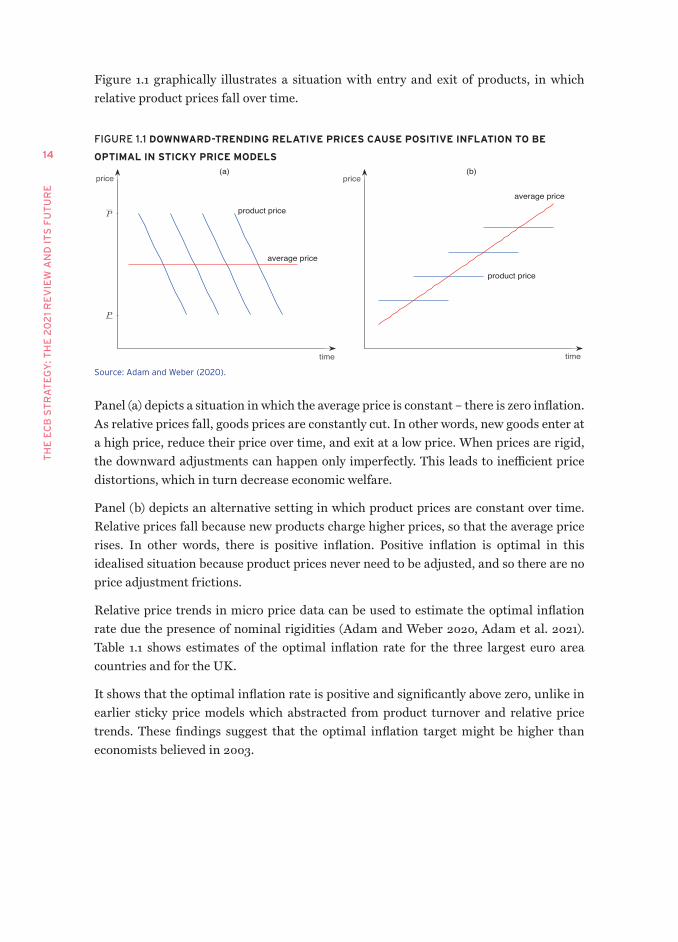
Figure 1.1 graphically illustrates a situation with entry and exit of products, in which relative product prices fall over time.
FIGURE 1.1 DOWNWARD-TRENDING RELATIvE PRICES CAUSE POSITIvE INFLATION TO BE
OPTIMAL IN STICKY PRICE MODELS
time
price
average price
product price
(a)
time
price
average price
product price
(b)
Source: Adam and Weber (2020).
Panel (a) depicts a situation in which the average price is constant – there is zero inflation. As relative prices fall, goods prices are constantly cut. In other words, new goods enter at a high price, reduce their price over time, and exit at a low price. When prices are rigid, the downward adjustments can happen only imperfectly. This leads to inefficient price distortions, which in turn decrease economic welfare.
Panel (b) depicts an alternative setting in which product prices are constant over time. Relative prices fall because new products charge higher prices, so that the average price rises. In other words, there is positive inflation. Positive inflation is optimal in this idealised situation because product prices never need to be adjusted, and so there are no price adjustment frictions.
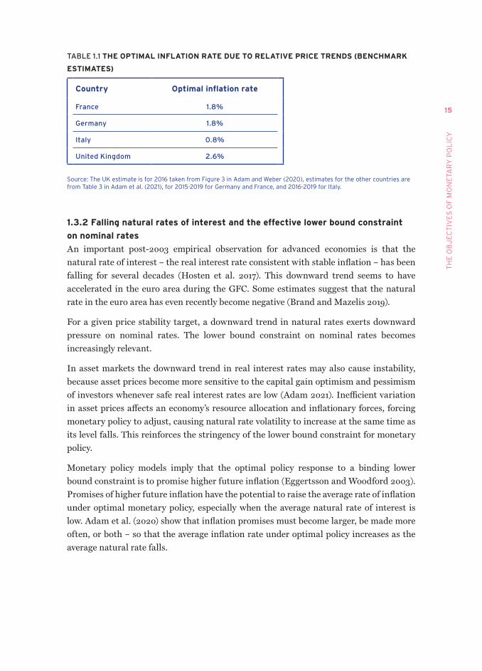
Relative price trends in micro price data can be used to estimate the optimal inflation rate due the presence of nominal rigidities (Adam and Weber 2020, Adam et al. 2021). Table 1.1 shows estimates of the optimal inflation rate for the three largest euro area countries and for the UK.
It shows that the optimal inflation rate is positive and significantly above zero, unlike in earlier sticky price models which abstracted from product turnover and relative price trends. These findings suggest that the optimal inflation target might be higher than economists believed in 2003.
15
TH
E O
Bj
EC
TIV
ES
OF
MO
NE
TAR
y P
OL
ICy
TABLE 1.1 THE OPTIMAL INFLATION RATE DUE TO RELATIvE PRICE TRENDS (BENCHMARK
ESTIMATES)
Country Optimal inflation rate
France 1.8%
Germany 1.8%
Italy 0.8%
United Kingdom 2.6%
Source: The UK estimate is for 2016 taken from Figure 3 in Adam and Weber (2020), estimates for the other countries are from Table 3 in Adam et al. (2021), for 2015-2019 for Germany and France, and 2016-2019 for Italy.
1.3.2 Falling natural rates of interest and the effective lower bound constraint
on nominal rates
An important post-2003 empirical observation for advanced economies is that the natural rate of interest – the real interest rate consistent with stable inflation – has been falling for several decades (Hosten et al. 2017). This downward trend seems to have accelerated in the euro area during the GFC. Some estimates suggest that the natural rate in the euro area has even recently become negative (Brand and Mazelis 2019).
For a given price stability target, a downward trend in natural rates exerts downward pressure on nominal rates. The lower bound constraint on nominal rates becomes increasingly relevant.
In asset markets the downward trend in real interest rates may also cause instability, because asset prices become more sensitive to the capital gain optimism and pessimism of investors whenever safe real interest rates are low (Adam 2021). Inefficient variation in asset prices affects an economy’s resource allocation and inflationary forces, forcing monetary policy to adjust, causing natural rate volatility to increase at the same time as its level falls. This reinforces the stringency of the lower bound constraint for monetary policy.
Monetary policy models imply that the optimal policy response to a binding lower bound constraint is to promise higher future inflation (Eggertsson and Woodford 2003). Promises of higher future inflation have the potential to raise the average rate of inflation under optimal monetary policy, especially when the average natural rate of interest is low. Adam et al. (2020) show that inflation promises must become larger, be made more often, or both – so that the average inflation rate under optimal policy increases as the average natural rate falls.
TH
E E
CB
ST
RA
TE
GY
: TH
E 2
02
1 R
EV
IEW
AN
D I
TS
FU
TU
RE
16
Andrade et al. (2019) reach a similar conclusion. They determine how the optimal intercept term in a Taylor rule should move with the average level of the natural rate of interest. They also show that inflation optimally increases as the natural rate falls. This suggests that the optimal inflation target is higher in a world with a lower average natural rate of interest.
1.3.3 New insights on menu costs
Research on costly price adjustment has made significant progress since the last ECB strategy review and provides important insights on how price-setting frictions interact with the inflation target. Menu cost models generalise standard time-dependent price adjustment models and can capture real-world price adjustment patterns. For instance, they capture well how prices adjust at different inflation levels (Alvarez et al. 2018). And so menu cost models offer an empirically credible theoretical framework for thinking about monetary policy.
The optimal price stability target in menu cost models is approximately the same as in models considering time-dependent price adjustment frictions (Adam and Weber 2020), but menu cost models offer additional insights into how price adjustment frictions interact with inflation. This is relevant if we want to understand the impact of an effective lower bound constraint and the ability to stabilise prices and output.
Alexandrov (2020) shows that, for menu cost models, positive trend inflation generates an important asymmetry in how the economy reacts to economic disturbances and policy actions: more positive inflation rates make prices upwardly more flexible in response to shocks, but downwardly more rigid.
So when there is higher trend inflation, it is easier to use policy to generate upward price pressure in response to shocks, but policy is less able to lift the real economy. Blanco (2021) shows that this causes significantly positive inflation rates to be optimal at an effective lower bound for nominal rates. Higher inflation is beneficial in welfare terms because it makes prices downwardly more rigid, which is desirable at the lower bound constraint. Higher inflation is desirable, even though the policy space created by higher inflation targets is partly counteracted by prices becoming endogenously more flexible (L’Huillier and Schoenle 2020).
Overall, the menu cost literature suggests that higher inflation targets are desirable if, in response to adverse economic disturbances, it is important to prevent prices from falling.
1.4 COMMUNICATING A HIGHER PRICE STABILITY OBJECTIvE
For an adjustment to the price stability objective to be effective, it needs to be communicated and executed in such a way that causes expectations of the public to shift over time to the new target level, and to remain anchored at that level. Part of this requires actually achieving inflation outcomes that satisfy the objective.
17
TH
E O
Bj
EC
TIV
ES
OF
MO
NE
TAR
y P
OL
ICy
Credibility is essential if the central bank seeks to anchor inflation expectations around its targeted inflation rate, as well as to control expectations of future interest rates. The monetary framework plays a central role in the establishment of credibility; but simply announcing a changed inflation target may not change inflation expectations, especially if the general public pays little attention to central bank communication. This reduces the central bank’s credibility.
It is vital that any change is communicated effectively. Financial markets, the main target for central bank communication, can understand the more nuanced arguments for the change, but it is important that they do not conclude that the central bank is abusing its ability to define its own target. This means that the ECB should commit to a schedule of reviews that are regular but not too frequent. To justify the use of its objective-setting power, changes should be lumpy and infrequent.
Communicating with the general public is more difficult. They know and understand less about monetary policy and are less engaged. When Coibion et al. (2020) analysed the effect of the Fed’s shift to average inflation targeting on the expectations of households, they found the new announcement had very little impact. If the benefits of changing the inflation objective depend on shifting those expectations, this strengthens the argument that we should change the objective only when there is a large change required, and at scheduled reviews. It also implies that the central bank will need to promote the change to the wider public, particularly through the media.
1.5 MAKE-UP STRATEGIES AND DYNAMIC ASPECTS IN ACHIEvING THE
PRIMARY OBJECTIvE
Monetary policymaking is dynamic, especially when economic agents are forward-looking. When future policy actions affect future outcomes, and economic agents factor these future outcomes into the economic decisions they make now, today’s economic outcomes are not independent of future policy choices. Forward-looking behaviour provides monetary policy with an inter-temporal dimension, and optimal monetary policy can use this dimension to spread the effects of economic disturbances over time (Woodford 1999).
Policymakers understand the gains of having well-anchored long-term inflation expectations, for example. When expectations about future inflation are anchored, there is a more favourable policy trade-off in response to economic disturbances today. At the same time, the need to fulfil these expectations – the need to keep inflation at the target over the medium term – constrains future policy choices. This causes optimal monetary policy to be history-dependent in a way that makes it time-inconsistent, because it is not consistent with optimality to engage in a purely forward-looking inflation targeting approach that seeks to maximise current and future economic outcomes unless policymakers also consider past expectations and promises (Kydland and Prescott 1977).
TH
E E
CB
ST
RA
TE
GY
: TH
E 2
02
1 R
EV
IEW
AN
D I
TS
FU
TU
RE
18
Recently, the ECB has not been able to reduce nominal interest rates and so has relied more on the intertemporal channel of monetary policy. This has meant that positive effects on current economic outcomes can largely only be achieved by promising to do things in future, by:
1. providing guidance on future nominal rates, perhaps backed-up by a corresponding path for asset purchases; and relatedly by
2. committing to letting inflation rise more than usual before lifting interest rates.
When agents correctly anticipate the promises – and the resulting economic inflation outcomes – those promises will reduce real interest rates and stimulate economic activity.
When economic disturbances lead to inflation rates below target and when monetary policy is – as a result – constrained in its ability to lower nominal rates further, it becomes optimal for monetary policy to keep interest rates lower for longer and to let inflation overshoot its usual targets for a limited period (Eggertsson and Woodford 2003, Adam and Billi 2006).
And so optimal monetary policy has features of the average inflation targeting approach adopted in August 2020 by the Federal Reserve System. Yet, it features an important asymmetry: in the presence of a binding lower bound constraint, the overshooting of inflation above its target is stronger than the undershooting that is optimal when economic disturbances push inflation above the target value. When there are negative shocks to inflation, it is optimal to let inflation rise more than one-for-one. The optimal response to shocks that drive inflation above target would be less than one-for-one.
This optimally asymmetric response might lift average inflation above the inflation rate usually targeted by the central bank in the absence of a binding lower bound constraint. This presents a difficult communication problem for the central bank. Moreover, the strength of the effect exerted by the lower bound constraint on average inflation depends on how severe a constraint the lower bound really is. In a world in which the average natural rate of interest has fallen significantly over time, the effect can be quantitatively quite important (Adam et al. 2020).
The average inflation rate under optimal monetary policy is thus a function of the severity of the lower bound constraint. If low average levels of the natural rate of interest are driven by low trend growth rates of the economy, this resembles a regime in which the central bank targets a path for nominal income/GDP (Woodford 2012). A nominal GDP path seems inconsistent with the goals of monetary policy set out in the EU Treaty. But an average inflation targeting or price-level targeting approach, using appropriate history dependence, will be close to such a policy, as long as the ECB accepts that the average inflation rate under optimal monetary policy must depend on the severity of the lower bound constraint.
19
TH
E O
Bj
EC
TIV
ES
OF
MO
NE
TAR
y P
OL
ICy
Overall, some form of make-up strategy is an important part of the optimal conduct of monetary policy. The make-up components may vary in stringency (average inflation targeting, price-level targeting), but not having any make-up component in the monetary policy framework would inevitably lead to a shortfall in the average inflation outcome below the stated inflation objective. Ironically, this means that even though the target is changed to be symmetric around 2%, the absence of a make-up strategy means that the ECB will likely end up achieving close to, but below, 2%.
For instance, a central bank that targets its inflation objective in a purely forward-looking way would deliver an average inflation outcome that falls short of its objective, with the shortfall being an increasing function of the degree to which the effective lower bound on nominal rates represents a policy constraint. It is likely this shortfall would be reflected over time in a shortfall in long-term inflation expectations. This, in turn, would further complicate the monetary stabilisation problem, because the lower bound constraint would become even more relevant.
This suggests that make-up strategies are important to anchor long-term inflation expectations. This is especially true in a world in which the natural rate of interest and the inflation target are both low, as the lower-bound constraint on nominal rates then becomes strongly relevant.
Clear communication of the different elements of the make-up strategy (the horizon over which the make-up is sought to be achieved, the size of the make-up and potential asymmetries in the make-up) can also help to steer the conditional inflation expectations of private agents beyond their long-term inflation expectations – though the analysis of Coibion et al. (2020) highlights the challenges of implementing any change.

21
CHAPTER 2
The tools of monetary policy at the ECB: A new normal
SUMMARY RECOMMENDATIONS
• The set of innovative policies that the ECB put in place since 2007 should be now considered as part of the new ‘normal’ operational framework. These policies include special lending programs, liquidity provision at a fixed rate, forward guidance, negative deposit rates, and purchases of both private and public assets. They work both as ‘substitutes’ of traditional short-term interest rate policy at the effective lower bound and as ‘complements’ in the presence of market distortions.
• We review evidence on their effectiveness and the conditions under which they have been successful. We make the point that a clear framework that uses all tools in a complementary way is the condition for effectiveness. We also discuss interactions between liquidity and monetary policy and conclude that the ECB should abandon the rhetoric of the ‘separation principle’.
• Given the relationship between policies affecting the size and composition of the central bank’s balance sheet and the euro area yield curve, we recommend summarising the monetary policy stance in terms of prices rather than quantities, and describe the intended policy impulse as the expected price effects onto the risk-free yield curve (captured by the OIS) at all maturities.
• The ECB should continue to actively monitor developments in sovereign and commercial debt markets as well as the emergence of liquidity risk in all segments of the market and consider using appropriate tools in order to compress spreads, if this is needed to smooth the transmission of monetary policy in line with its price stability objective and with its secondary objective of financial stability. Given the still prevailing segmentation of markets along national lines and the correlation between sovereign and banks’ risks, this is particularly important in the euro area. Transparent communication on the targets pursued and related motivation is a condition for credibility and effectiveness of such policies.
• The ECB should use the deposit rate as the main short-term policy rate.
• It should not rely on rating agencies when pricing collateral but determine its own criteria.
• It should clarify the future availability and goals of swap facilities.
TH
E E
CB
ST
RA
TE
GY
: TH
E 2
02
1 R
EV
IEW
AN
D I
TS
FU
TU
RE
22
• It should limit the recourse to ELA considering – as stated – extraordinary facilities.
• It should clarify criteria for choosing asset compositions against digital currency, which requires the analysis of the interaction between digital euro and monetary policy.
INTRODUCTION
Before the global financial crisis (GFC) of 2008, the central bank balance sheets in most advanced economies received little attention. This included the balance sheet of the ECB.
Its size was around 10-15% of GDP, with small fluctuations from year to year. The major items on both the liabilities side (currency) and the assets side (foreign assets and gold) were not actively used or discussed in standard policy setting. It was acknowledged that the balance sheet might have to vary in size, as banks changed their demand for lending from the ECB, but this was a passive policy: the ECB was responding to circumstances rather than actively choosing its size, acting as a liquidity provider and lender of last resort. There was a ‘separation principle’ that these liquidity measures would be temporary and focused on financial stability. This was distinct from proper monetary policy.
The ECB conducted its operations using the marginal repurchase operations (MRO), a programme through which banks give financial assets to the central bank (picked from a collateral list set by the ECB and, again, rarely discussed), and receive deposits at the central bank in return, promising to repurchase the assets and return deposits plus interest within one week. The resulting changes in the monetary base were moderate: they were a consequence rather than a driver of policy.
The main target was inflation and the main instrument to affect it was to move the short-term interest rate on the MRO and, through this, the other short-term safe interest rates throughout the euro area. Key discussions centered on how to change this policy rate, often framed in terms of some feedback rule from inflation, plus indicators of real activity or financial stability.
Research and analysis were devoted to understanding how changes in safe, short-term interest rates affected riskier and longer-term interest rates, and how they were transmitted to the economy, thus allowing the central bank to manage fluctuations in credit and savings and, through them, inflation.
While this conventional description of monetary policy may still dominate in textbooks, it is woefully out of date. This description has not fit the ECB’s policy in more than a decade. Hartmann and Smets (2018) and Rostagno et al. (2019) describe the changes in how the ECB conducted monetary policy, and how they came about over time. There are so many of them that it takes these authors hundreds of pages to discuss them, with
23
TH
E T
OO
LS
OF
MO
NE
TAR
y P
OL
ICy
AT
TH
E E
CB
: A N
EW
NO
RM
AL
tables that sometimes span more than one page to list them. For what is now more than half of its existence, the ECB has deviated from what is still referred to in discussions as the norm, or what is traditional. It is also unlikely that monetary policy in the euro area will resemble the description above any time soon. The ECB has now communicated that the tools developed in the last decade are here to stay as long as economic circumstances justify it. However, the ECB message – as far as we understand – is still that these operations are ‘exceptional’. We believe that the ECB should clarify that the need for the use of these new instruments will remain and that therefore they must be part of a ‘new normal’ . Explaining what the new normal looks like is important for at least (three) reasons:
1. Credibility. Perpetually discussing the present as being ‘exceptional’ and not traditional poses a serious risk to credibility.
2. Norm-setting. The review sets the norm and provides a link to the Treaties to which legal challenges and disputes to the ECBs actions can refer.
3. The old days are unlikely to come back. If used repeatedly, the programmes should be described as recurrent policies rather than temporary ones. If not, their effectiveness is compromised. If the toolkit has changed, this should be acknowledged and discussed without longing for the return of old times.
This chapter discusses what this new traditional toolkit should be. It starts by discussing the scope and rationale of the various tools which affect the size and composition of the balance sheet. Then we analyse them individually: the tools to control short-term rates, the influence over longer-term rates, the asset purchases programmes, lending and liquidity programmes, and digital currencies. We suggest that this complex new operational framework should be translated in a yield curve objective. This is followed by a section on empirical evidence and a brief conclusion.
2.1 THE RATIONALE FOR POLICIES OTHER THAN SHORT-TERM RATE-
STEERING
The policy tools developed by the ECB since the financial crisis are sometimes generically called ‘balance sheet policies’, although they involve not only asset purchases but also special lending programmes and forward guidance. To the extent to which they affect the size and composition of the central bank’s balance sheet, they affect the relevant interest rates and risk premia.
TH
E E
CB
ST
RA
TE
GY
: TH
E 2
02
1 R
EV
IEW
AN
D I
TS
FU
TU
RE
24
There are two distinct rationales for balance sheet policies:
1. To provide liquidity to the market in times of financial stress. At these moments the whole financial system may want to shift into safe liquid reserves. The lack of market liquidity when everyone is trying to sell assets may lead to fire-sales of assets, triggering a financial crisis. By providing liquidity, the central bank can ameliorate or even avoid such panics.
As a consequence, the central bank’s balance sheet increases endogenously in size, causing spreads between yields of risky and less risky securities (for example, between secured and unsecured interest rates) to compress, relative to a situation where increased liquidity demand were not accommodated. We can define these policies as ‘passive’ because the increase in balance sheet size is the consequence of the bank’s liquidity policy. They thus complement traditional short-term interest rate policy.
Providing liquidity in response to a liquidity crisis is known as ‘Bagehot’s Principle’ and is part of a traditional central bank toolkit. In theory, the bank will ‘lend freely against good collateral’ and not take credit risk. In practice, there is some ambiguity, since the principle requires that we can identify solvency and liquidity in real time (for a discussion of this issue in the context of ECB policy, see Reichlin 2014, Pill and Reichlin 2015 and Reichlin 2019).
The Long Term Refinancing Operations (LTRO) programme implemented in 2008-2009 is an example of these policies in the euro area. The central bank effectively replaced the inter-bank market by issuing special loans to banks at fixed rate and in full allotment. The ECB’s balance sheet expanded endogenously by increasing reserves on the liability side against (largely) conventional assets (repos) on the asset side. Other examples are the longer-term and targeted refinancing operations, such as TLRO-I, LTRO-II and TLTRO-III, implemented later, and the pandemic emergency longer-term refinancing operations (PELTRO). These programmes have considerably expanded the role of the ECB as an intermediary.
2. To provide alternatives to conventional interest rate policy. These are employed when the short-term interest rate has reached or neared an effective lower bound (ELB) for the policy rate. In such a case, asset purchase programmes are interventions meant to ease the financial conditions faced by the private sector once the scope for conventional monetary easing (lowering the level of short-term interest rate) is exhausted or very limited. This type of measure is aimed at lowering yields on safe assets at longer maturities, pushing investors further along
25
TH
E T
OO
LS
OF
MO
NE
TAR
y P
OL
ICy
AT
TH
E E
CB
: A N
EW
NO
RM
AL
the risk and maturity spectra. They address the macroeconomic implications of crises. We define these measures as ‘active’ since, in this case, the central bank acts deliberately to change the size of its balance sheet (Pill and Reichlin 2017, Reichlin 2021).
We can think of forward guidance and negative interest rates as further categories of unconventional monetary policy. They are complementary to asset purchases because they act on different parts of the yield curve (indeed, the ECB has stressed their complementarity). These policies were implemented later in the euro area: the corporate bond purchase programme in late 2014 and then the government bond purchases (APP) in early 2015, although a limited experiment had been tried in 2010-2011 with the Securities Market Programme (SMP); the Outright Monetary Transaction (OMT) programme was announced in 2012 but never implemented. The recent Pandemic Emergency Purchase Programme (PEPP) also falls into this category.
In general, with passive policies the central bank acts as a market maker and, by doing so, increases the liquidity of the assets. With ‘active’ policies the central bank becomes a market participant – an investor with inelastic demand – and by doing so absorbs risk from the market, swapping safe reserves for risky debt securities. This causes a compression in interest rate spreads which reduces borrowing costs for firms and governments. The mechanism is likely to be particularly relevant when those governments are under a spending constraint or market pressure.
Under what conditions are these policies effective? In theory, it is not difficult to explain the effectiveness of the ‘market maker’ policy since, in that case, the central bank removes a friction created by market disruption. In so doing it supports channels of financial intermediation that are important for both financial stability and macroeconomic objectives by lending to different sectors in the economy. Reichlin (2019) argued that these programmes were successful in supporting credit when the origin of the problem was liquidity, but less so later when the problem was solvency of a large part of the euro area banking sector (Giannone et al. 2012 and Colangelo et al. 2017 provide quantitative empirical evidence on this point).
Macroeconomists struggle to identify whether active policies have been effective and to measure their impact. In theory, a change in the relative supplies of assets in the hands of the private sector should have no effect on equilibrium quantities and asset prices, absent financial frictions. For them to work, there must be mechanisms that make assets of different maturities imperfect substitutes. If this is the case, this neutrality proposition breaks down. In this case, asset purchases can affect long-term interest rates by reducing the risk premium, therefore relaxing financial constraints when they would otherwise be binding.
TH
E E
CB
ST
RA
TE
GY
: TH
E 2
02
1 R
EV
IEW
AN
D I
TS
FU
TU
RE
26
Another important mechanism that could explain the effectiveness (or otherwise) of asset purchases would be the signal that the central bank will keep the short-term interest rates low once the zero lower bound ceases to be a constraint (Woodford 2012). Forward guidance and asset purchases must then be understood as being complementary.
The effectiveness of both policies – active and passive – is related to the extent to which market imperfections and financial frictions are pervasive. The tools are likely to be more effective in financial crises when markets are distressed, but they may also be effective in normal times when markets fail to operate efficiently for other reasons.
2.1.1 Special considerations in the euro area
There is an extra dimension to monetary policy in a monetary union. The policies we have discussed affect the ‘common’ risk free yield curve (typically proxied by the OIS curve), as well as risk premia associated to country-specific yield curves (countries face their own default risk).
Intervening in the sovereign bond market via asset purchases has two functions. The first is to achieve favourable long-term financing conditions for the public and private sector by flattening the risk free yield curve. When financial markets are functioning well, the effect of this policy is likely to be small, as arbitrage largely neutralises the price effects. With imperfect substitutability across the maturity spectrum or when purchases signal policy intentions regarding the future interest rate policy, these interventions can affect long-term yields. The second function is to address tensions in specific government bond markets, which can be justified on the grounds of addressing financial fragmentation and specific financial frictions at the geographical level. Such policies, however, come close to financing some governments and therefore must be well justified in terms of the specific frictions that policy seeks to address.
Non-standard monetary policy is also effective in the euro area because member states do not issue their own money, and so are vulnerable to liquidity crises. When these crises occur, the central bank has an important stabilising role, especially because the crises may become self-fulfilling and lead to multiple equilibria. In these situations, the central bank can act or even signal that it will act, which may switch the economy from a bad to a good equilibrium (Corsetti and Dedola 2016, Bocola and Dovis 2019, Lorenzoni and Werning 2019).
A classic example of such a phenomenon is the spike in interest rates of Italian and Spanish sovereign bonds during the debt crisis. Willingness to act as in 2012 (Draghi’s speech pledging to do “whatever it takes to save the euro” and announcing the OMT programme) signalled commitment to intervene in the market that prevented the liquidity crisis spiralling into a solvency crisis.
27
TH
E T
OO
LS
OF
MO
NE
TAR
y P
OL
ICy
AT
TH
E E
CB
: A N
EW
NO
RM
AL
Even during periods of extreme stress, as in the period 2010-2012, negative macroeconomic shocks in the monetary union typically lead to the double phenomenon of flight to safety (a flight to the German bund, in particular, by foreign investors) and home bias in sovereign purchases, causing financial market fragmentation along geographical lines.
This occurs because there is no euro area safe asset and because there is imperfect financial integration, particularly in retail financial services. In addition, the prospect of a potential euro area break-up looms in the background. The ECB has emphasised that these features may impair the transmission mechanism of monetary policy by creating geographical heterogeneity of financial market conditions. In these circumstances, nonstandard policies, by acting to ease constraints in specific markets, are potentially very effective.
But this does not mean we should always and unconditionally choose policies aimed at compressing cross-country spreads. Although spreads may in part reflect financial frictions and self-fulfilling dynamics, they also reflect differences in bond default probabilities. The liquidity and solvency attributes, however, are difficult to separate, which creates a problem in defining a policy target for the ECB based on monetary policy considerations only. We discuss this below.
2.2 THE SIZE OF THE BALANCE SHEET AND THE SUPPLY OF RESERvES
It is an accounting identity that the size of the balance sheet is equal to the central bank’s net worth plus its liabilities. We know also that the liabilities of a central bank consist almost entirely of currency plus bank deposits at the central bank – both direct deposits, and one side of the repurchasing operations.
The ECB, like most central banks, is bound by a rule to remit its net income to the national central banks, and eventually to the Treasuries in those countries. It can deviate from this rule by provisioning and, more substantially, it has some discretion in adopting accounting rules that smooth out net income across years. The ECB has a peculiar rule in this category: it keeps the net income from capital gains in the holdings of foreign currency, putting them in a ‘revaluation account’ rather than counting them as net worth. These deviations are either small or not a policy choice, so net worth is approximately constant from year to year.
The amount of currency in circulation is also not chosen by the ECB. Rather, it commits at all dates to exchange deposits that banks hold at the ECB for currency one-to-one. Across seasons, economic agents sometimes want to hold more currency, and other times less. If currency were exogenously set by the central bank, this would lead to large seasonal fluctuations in interest rates and inflation, as the opportunity cost of holding
TH
E E
CB
ST
RA
TE
GY
: TH
E 2
02
1 R
EV
IEW
AN
D I
TS
FU
TU
RE
28
currency would have to adjust to clear the market. Almost all central banks in advanced economies passively accommodate these shifts in demand by exchanging currency for deposits, and so they cannot choose to change the size of the balance sheet through currency.
Therefore, a discussion of the size of the ECB balance sheet is a discussion of the size of the reserves (deposits plus MRO credits) that commercial banks have on the ECB. The ECB can control this perfectly, because it can increase or shrink these reserves by simply changing the digital entries on each counterparty’s account in its deposit spreadsheet. In exchange, the ECB receives either financial claims on the banks, or on other agents that the bank has given to the ECB.
Increasing the supply of reserves means that their opportunity cost falls. Instead of depositing or borrowing from the central bank, banks can borrow and lend to other banks. The difference between the interbank rate and the interest rate on the reserves gives this opportunity cost.
Once the supply of deposits grows large enough, the opportunity cost falls to approximately zero, as it did in the euro area some years ago. Economists would say that the demand for reserves was satiated, or that the market for reserves was saturated.
The old ECB regime would auction a fixed amount of loans at the MRO rate. Since 2008, the ECB has instead held a variable tender auction at a fixed rate, effectively supplying an unlimited amount of reserves at this rate. Keeping the MRO at full allotment forever is referred to as producing a ‘structural liquidity surplus’. With a small difference between the MRO rate and the deposit rate (or maybe none at all), this has meant the market for reserves has been saturated in the euro area for more than 10 years.
Importantly, this new regime increases the size of the balance sheet with no change in current or expected interest rates, thus it has approximately no effect on expected inflation. Since demand is satiated, the extra reserves have no effect on expected liquidity premia (unless it acts as a signal about future interest rate policy). At the date of the announcement of the increase in reserves, but before it happens, there is also no clear impact on real interest rates. With no change in the nominal interest rate, then the Fisher equation implies that expected inflation is also unchanged.
While this theoretical thought experiment will rarely – if ever – hold exactly, it shows clearly that, as happened during 2020, the ECB can massively increase the size of the balance sheet to respond to emergencies without losing control of its interest rate and inflation targets.
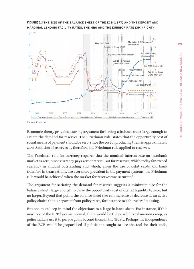
29
TH
E T
OO
LS
OF
MO
NE
TAR
y P
OL
ICy
AT
TH
E E
CB
: A N
EW
NO
RM
AL
FIGURE 2.1 THE SIZE OF THE BALANCE SHEET OF THE ECB (LEFT) AND THE DEPOSIT AND
MARGINAL LENDING FACILITY RATES, THE MRO AND THE EURIBOR RATE (3M) (RIGHT)
2000 2002 2005 2007 2010 2012 2015 2017 20200
1
2
3
4
5
6
7 106
-2
-1
0
1
2
3
4
5
6
7
May 2010: SMP
Dec 2011: 3-year LTRO
July 2012: "whatever it takes"
July 2013: Forwardguidance on rates
June 2014: Negative rates
Jan 2015: QE announced
March 2015: start QE
March 2016: QE expanded
Jun 2018: End ofQE announced
Dec 2018: End of QE
Sep 2019: Restart
Mar 2020: PEPP
Eurosystem Assets Deposit Facility rate Marginal Lending Facility rate Main Refinancing Operations rate Euribor rate (3M)
Source: Eurostat.
Economic theory provides a strong argument for having a balance sheet large enough to satiate the demand for reserves. The ‘Friedman rule’ states that the opportunity cost of social means of payment should be zero, since the cost of producing them is approximately zero. Satiation of reserves is, therefore, the Friedman rule applied to reserves.
The Friedman rule for currency requires that the nominal interest rate on interbank market is zero, since currency pays zero interest. But for reserves, which today far exceed currency in amount outstanding and which, given the use of debit cards and bank transfers in transactions, are ever more prevalent in the payment systems, the Friedman rule would be achieved when the market for reserves was saturated.
The argument for satiating the demand for reserves suggests a minimum size for the balance sheet: large enough to drive the opportunity cost of digital liquidity to zero, but no larger. Beyond that point, the balance sheet size can increase or decrease as an active policy choice that is separate from policy rates, for instance to achieve credit easing.
But one must keep in mind the objections to a large balance sheet. For instance, if this new tool of the ECB became normal, there would be the possibility of mission creep, as policymakers use it to pursue goals beyond those in the Treaty. Perhaps the independence of the ECB would be jeopardised if politicians sought to use the tool for their ends,
TH
E E
CB
ST
RA
TE
GY
: TH
E 2
02
1 R
EV
IEW
AN
D I
TS
FU
TU
RE
30
for instance dictating that the ECB issue more reserves to provide credit to favoured industries or activities. None of this is an objection to the principle of saturating the market for reserves, or to quantitative or credit easing. But these dangers must be taken into account.
2.3 THE INTEREST RATE TOOL(S)
The old ECB regime would auction a fixed amount of loans at the MRO rate while setting a deposit rate below the MRO rate. This implied that the supply of reserves was scarce, and the central bank deposit rate was below the private interbank market rates. An upper ceiling on those rates was given by a lending rate also set by the ECB through its marginal lending facility, at which banks could get euros with less collateral requirement than the MRO.
Now, with variable tender auctions at the MRO to satiate the demand for reserves, the central bank is operating what is sometimes called a ‘floor system’ when setting interest rates. For the past 13 years, the interbank rates of similar maturities and safety have become very close to either the MRO or the deposit rate.
A floor system is likely a better way to conduct monetary policy. It removes the risk of operational error when trying to fix the right quantity of MRO operations to hit an interest rate target. It implies that sharp increases in the demand for reserves at the central bank, as happens around financial crises, can be automatically accommodated by the ECB. More significantly, it allows for QE policies to be pursued as a complement to setting interest rates.
In a corridor system, the interest rate and the size of the balance sheet are married. All else equal, raising the size lowers the interest rate, and vice versa. In a floor system, they are divorced. The central bank can, on top of the MRO, make outright purchases of financial assets in exchange for an increase in the deposits of the seller of those assets at the ECB.
Before this system was implemented, policymakers worried that it would disrupt money markets or the liquidity management of banks. The strong evidence of the last 13 years is that saturating the market for reserves is sustainable with little significant downside risk to financial markets. Money markets did not close in any country that has adopted this system.
The ECB has gone further in the last decade, introducing a set of different interest rates. There is a deposit rate that banks receive for their deposits at the ECB, which are partly voluntary and partly needed to satisfy regulatory requirements. The interest rate is tiered to reflect these two types of reserves: required reserves have paid a negative interest rate for years, while voluntary reserves greater than a multiple of the required reserves are remunerated at zero interest rate. Then there is the MRO rate, at which banks can briefly park their financial assets in exchange for euros. There are also long-
31
TH
E T
OO
LS
OF
MO
NE
TAR
y P
OL
ICy
AT
TH
E E
CB
: A N
EW
NO
RM
AL
term refinancing operations (LTROs), with a maturity of three months, and operations with maturities in years such as the PELTROs (pandemic emergency LTROs) adopted in 2020 and the TLTROs (targeted) that require banks to meet criteria in the use of the funds to make loans.
The ECB should clarify which of these rates is the main instrument of monetary policy. The best choice is perhaps the deposit rate. It is set independently of other considerations (it is not affected by the size of the balance sheet, collateral lists, maturity, or other requirements). It matches the short-term safe remuneration on the unit of account for which a central bank is ultimately responsible. It would be the primary tool of the central bank, as it is at the heart monetary policy theory.
The secondary toolkit of interest rate policies – tiering exemptions, MRO collateral list and haircuts, LTRO rates and requirements – could all be chosen with reference to the deposit rate. So far the evidence on their relative importance is mixed and often confusing, and the ECB should invest more effort to research this question. These secondary choices clearly have an effect in financial markets, but no one has quantified their impact in the transmission mechanism of policy across interest rates and credit conditions, or linked this to inflation or real activity. There are no clear downsides to having these extra tools. Listing them, and the ECB’s view of their impact, would normalise their use.
Finally, there is a debate on whether the deposit rate could be set at negative values. Most of the evidence today suggests that cutting rates below 0% still has an expansionary effect on credit, real activity, and inflation, although confidence intervals are wide. Therefore, it would be unwise to rule them out. But there is a limit (and effective lower bound) on how low negative rates can go before banks start turning down depositors, or people start converting digital deposits into physical currency that pays no interest.
2.4 LENDING PROGRAMMES
Central bank lending to banks has three purposes:
1. To satisfy short-term commitments. Individual banks occasionally need reserves or currency to satisfy either regulatory requirements or sudden withdrawals of deposits by the end of the day but lack the time to find a lender in the interbank market. A standing marginal lending facility at the central bank can prevent failures to satisy these commitments.
2. To reduce the risk of bank runs. Banks transform maturity, borrowing short to make long and illiquid investments, exposing them to the threat of bank runs. By offering a lending facility against runs on deposits driven by either unusual demand by customers for means of payment or by depositor panics, the central bank can provide some tail insurance to banks.
TH
E E
CB
ST
RA
TE
GY
: TH
E 2
02
1 R
EV
IEW
AN
D I
TS
FU
TU
RE
32
3. To be a bulwark in a crisis. In a systemic crisis, the central bank can accommodate the demand for a safe asset by acting as lender of last resort (see Section 2.1).
Before and during the crisis, the ECB stressed that liquidity management policies were distinct from monetary policy. This is the separation principle. The rate set for the MRO was determined by monetary policy, while the amount lent using it, or using the marginal lending facility, was an outcome of liquidity policy. By extension, when the LTRO were introduced at the end of 2011, this was also a liquidity policy.
Recently this separation has become less distinct. Also, as we have shown, the separation as it has worked so far also appears unsustainable.
Saturating the market for reserves provides ample liquidity to the banking sector. Liquidity has been dealt with through the Friedman rule, and so it no longer needs to be actively managed. The large stock of outstanding reserves ensures that the increase in the demand for liquid safe funds during a financial crisis is likely to be met by an abundant supply. If interest rates are at the floor rather than in the middle of a corridor, they are less likely to hit the ceiling if lending of last resort is needed. This is as much of a liquidity policy as it is the monetary policy that we discussed earlier in this chapter.
Likewise, as discussed, both QE and LTROs are about lowering long-term rates. The channels may be different, but they would both be monetary policies in a ‘going long’ framework. Even if a world existed in which LTROs would be strictly used for lending of last resort, that has not been the reality in the euro area. It is not even clear that this alternative would be a better world. We are happy to see that the separation principle does not appear any longer in ECB communication. We expect that when the background papers of the ECB review are published, the separation principle will be jettisoned.
In globalised financial markets, banks often operate across borders under the jurisdiction of different central banks, making investments and borrowing in different currencies. During the financial crisis, non-US banks making investments in dollars found themselves unable to roll over dollar funding in financial markets. The Federal Reserve stepped in by creating and expanding a new type of central bank swap lines, lending dollars to a foreign bank so that it could disburse them to its banks, preventing a fire sale of dollar assets.
In 2008-10, the ECB was reluctant – and slower – to create similar facilities for countries, mostly in Eastern Europe, in which financial institutions had been very active in euro markets. Since then, the ECB has expanded its network of swap lines, including significant lines with the Bank of England and the People’s Bank of China. During March and April 2020, the Federal Reserve greatly expanded its dollar network in response to Covid-19, and the ECB likewise was faster to ensure access to euros outside the euro area.
33
TH
E T
OO
LS
OF
MO
NE
TAR
y P
OL
ICy
AT
TH
E E
CB
: A N
EW
NO
RM
AL
Swap lines remain a discretionary policy, for which terms are negotiated individually with the counterparty central bank. A mission review might clarify the ECB’s views on the future availability and goals of these facilities. It is not clear whether this has been the case.
During the financial crisis, national central banks within the Eurosystem used Emergency Liquidity Assistance (ELA). This consisted of loans to national financial institutions under severe stress against collateral decided by the national central bank. This turned out to be important for institutions that either did not have the collateral that the ECB would accept in its own lending facilities, or that appeared to be near failing but were important for national financial stability in the opinion of the national central bank. The ECB must be informed when ELA is used, and can block national actions if two-thirds of the governing council objects to it. ELA is a last remnant of national monetary sovereignty. It is, and should remain, extraordinary. If abused, it would undermine the ability of the ECB to implement monetary policy.
2.5 SIZE OF THE BALANCE SHEET AND COMPOSITION OF THE ASSETS
In its first decade, the ECB’s balance sheet was composed of two main categories of roughly similar size, and a smaller third category:
1. Credits on banks through MROs and LTROs. These were backed by the financial assets these gave in the repurchase agreements.
2. Gold and foreign currency. This was given to the ECB by national governments when it was first capitalised and has remained relatively stable.
3. A smaller residual. Some securities held outright and other assets.
The composition of the ECB’s portfolio of assets has changed greatly. In the last decade the ECB’s assets have increased, first because of its special lending policies in 2008, then as a result of the Security Market Programme (SMP) in 2010. The portfolio shrank between 2012 and 2014 as banks repaid their loans, and increased during the QE programme of 2015, and especially in 2020 with the asset purchase programme implemented to fight the pandemic (Figure 2.1).
Initially the increase was in refinancing operations through the MRO and especially the different versions of LTROs. These credits to banks absorbed financial securities from the financial sector, pledged as collateral against loans. The management of assets in this collateral list can be an important policy lever. The central bank applies a haircut to each asset to reflect the risk from changes in the value of asset during the contract.
TH
E E
CB
ST
RA
TE
GY
: TH
E 2
02
1 R
EV
IEW
AN
D I
TS
FU
TU
RE
34
Adjustments in these haircuts can have a large effect on the liquidity of the asset in financial markets, because they can be pledged at the central bank at any time as part of one of the refinancing operations. These assets trade at a higher price, and if they are removed from the list this imposes a cost on its holders and issuer.
The collateral list used by the ECB for repurchase operations is pre-announced, and the haircuts follow conventional risk-management approaches. But the system has been criticised for its reliance on private credit agencies. With sovereign downgrades (sometimes justified, sometimes contentious, sometimes lagging actual developments), these private firms can exclude important parts of the Eurosystem financial system from the collateral list. This severely limits the ability of the central bank to retain the integrity of the euro.
Moreover, since sovereign credit ratings are often lagging reflectors of changes in market prices, having a collateral framework that depends on market prices creates a dangerous self-fulfilling run equilibrium on sovereign debt in the euro area. During sovereign debt crises, ECB policy towards its collateral list can have great significance: the exclusion of a group of financial assets from the list, by dramatically reducing their liquidity in markets, can make financial panics more likely or more serious. Market discipline is important for the no-bailout clause of the Maastricht Treaty, but implementing it strongly through the collateral framework of the ECB hampers monetary policy and endangers financial stability. We encourage the ECB to set out plans for replacing credit ratings with an alternative. This would be an important step forward for the euro area.
From the MRO to the PEPP, there was a gradual policy shift: from passive balance sheet policies in which the central bank accommodated changes in demand for liquidity, to policies in which the central bank is an active market participant – an investor with inelastic demand – and by doing so absorbs risk from the market, swapping safe reserves for risky debt securities.
The other large increase in the assets of the ECB has been in the amount of securities held outright. The first experiment was in 2010 with the Securities Markets Programme, later discontinued. The “whatever it takes” Outright Monetary Transactions (OMT) programme introduced in 2012 was not used. The growth in securities came after 2014 with the adoption of an asset purchase programme through which the ECB bought financial assets from banks, crediting their deposit account at the ECB.
Unlike in other advanced economies, there are no euro area-wide sovereign bonds spanning the maturity structure that the ECB can directly buy. As a result, its purchase of government bonds (the public sector purchase programme, or PSPP) must choose not just the maturity of what to buy, but also its national origin. Moreover, the ECB has opted to buy significant amounts of covered bonds (the third covered bond purchase
35
TH
E T
OO
LS
OF
MO
NE
TAR
y P
OL
ICy
AT
TH
E E
CB
: A N
EW
NO
RM
AL
programme, or CBPP3), corporate bonds (the corporate sector purchase programme, CSPP) and asset-backed securities (the ASDPP). The choices of what to buy among, and within, them are even broader. To these were added the pandemic emergency purchase programme (PEPP), which has significantly increased the size of the balance sheet.
We have argued that these policies may be effective in the presence of financial market imperfections and for that reason should remain. But it is not easy to communicate the rationale for this complex set of policies. We will return to this point.
2.6 PRESENT AND FUTURE RATES
During its first decade of existence, the ECB set interest rates systematically. Interest rates were expected to fall if inflation was expected to be below target, either because inflation was currently low or because real activity seemed depressed relative to the economy’s potential. Judgement was used on the state of the economy and on its likely path in the near future, as well as on whether other financial conditions merited looser or tighter policy.
A governing council expressed their individual judgements, and an interest rate decision was made collectively. This meant monetary policy was systematic and rules-based, even if it was not predictable or rules-constrained. The members of the governing council complemented their choices with speeches and other communication on the outlook for the economy and for monetary policy. Changes in policy therefore affected both current short-term rates and their expected path, moving long-term rates as well and transmitting policy changes more effectively to credit conditions.
This process worked excellently for price stability. The HICP in January of 2009 was almost exactly equal to 1.0210 of its value in January of 1999. If the state of the world allows for it, returning to this condition should be part of the mission of the ECB.
In the last decade, however, the state of the world has not allowed it, and this continues to be the case. As real interest rates fell in advanced economies, the effective lower bound became binding, preventing central banks from lowering policy rates. They have become stuck at this lower bound. Real natural rates of interest are expected to remain low for a few years, perhaps longer. The ability of a central bank to move the policy rate is the bedrock of monetary policy, but recently the ECB and other advanced central banks have not been able to do this.
Central banks can still use one tool from the old playbook: they can communicate on what future policy rates will be when the constraint is no longer binding. This forward guidance has become the most important part of interest-rate policy in the last decade. It was first explicitly stated in July of 2013, although communicating about future interest rates has always been part of the ECB modus operandi.
TH
E E
CB
ST
RA
TE
GY
: TH
E 2
02
1 R
EV
IEW
AN
D I
TS
FU
TU
RE
36
An immediate effect of announcing lower future short-term interest rates would be to lower longer-term interest rates through arbitrage. This provides an immediate stimulus to credit and economic activity. If the central bank is able to steer the market expectations of the future with its announcements, then this a powerful lever with which to keep on pursuing the mandate and controlling inflation – even when interest rates are at the effective lower bound. The ECB’s review stated that it will continue to use forward guidance, and it has clarified that it will do so using state-contingent statements for its interest rates. This is a welcome normalisation.
2.7 CENTRAL BANK DIGITAL CURRENCY
The ECB plans to create a digital euro soon. This will be an electronic means of payment that, like currency, is available to any citizen and, like reserves, is digital and sits on the ECB’s balance sheet. It is not a replacement for either. Rather, it will be a complement, providing an alternative way to make payments in the euro area.
Satiation of bank demand for reserves is a necessary first step to expand access to the balance sheet to other economic agents. Once the ECB issues digital currency to citizens in the euro area on demand, it is hard to see how it could limit access to deposits or MRO to banks. This would be both practically difficult and would create unhelpful distortions.
Monetary policymakers must decide whether digital euros would pay interest. This will determine their role in the transmission of monetary policy. A digital euro with a fixed zero interest rate would presumably also raise the effective lower bound. If it was offered with few limits or fees, it would even raise the bound all the way to zero. Citizens and banks alike would have a more attractive alternative to bank reserves at the central bank. Any discussion on the feasibility of negative interest rates is therefore tied to the design of the digital euro.
A digital euro would also change the ECB balance sheet. If the digital euro is a success, it would considerably increase the liabilities on the ECB’s balance sheet. This need not interfere with monetary policy but, if the conventional central bank practice is followed of holding assets against currency, then what do we use for these assets? A close-to-neutral choice would be to hold only very short-term sovereign bonds. But, in pursuit of going-long policies, the ECB could decide to hold assets to allow it to affect longer-term interest rates.
A digital euro poses many other questions for payment systems. We can find answers to those question in speeches made by members of the ECB governing council. Future reviews should formalise the interaction between the evolution of payment systems and monetary policy.
While the introduction of a digital euro is likely to enlarge the policy space available to the ECB, a full discussion of the implications of digital currency is beyond the scope of this review.
37
TH
E T
OO
LS
OF
MO
NE
TAR
y P
OL
ICy
AT
TH
E E
CB
: A N
EW
NO
RM
AL
2.8 QUANTITIES AND PRICES: A UNIFIED FRAMEWORK
The choice across these different policies, and so across the composition of assets for the ECB, is complex. The ECB calibrates it policy stance by selecting the size of the interventions, the mix of LTROs versus APP, the different types of LTROs and associated collateral list of haircuts, the source and maturity of the national bonds to buy, and the basket of corporate and covered bonds to hold. It also must choose – and be clear about providing – forward guidance on the expected policy paths across each of these dimensions if it wants to steer expectations and prevent costly market tantrums.
With such a multidimensional policy space, the ECB faces the significant challenge of trying to communicate what is guiding these QE policies and to evaluate their success. If we are not certain how effective the policies are, it is hard to calibrate the menu ex ante, or to adjust it ex post. Providing a common framework of reference for all these programmes is important, but how can we do it?
There is a common thread running through the speeches made by members of the governing council about QE. They often (not always) explain the effectiveness of the policies in terms of their effect on long-term rates. In turn, they describe asset purchases as a complement to forward guidance, sharing the goal of affecting interest rates of longer maturities.
The unifying principle behind policies is therefore a focus by the central bank on moving interest rates further along the yield curve.
Discussing the menu of policies with explicit reference to the yield curve, or at least to a long rate, would provide these policies with a common denominator. Going long but staying focused on interest rates would improve transparency and communication. This would be consistent with the way the central bank tries to affect short-term interest rates, as discussed. At present QE policies are often reported in terms of quantities. Future reviews should change this.
It is awkward to have a central bank that, on the one hand, focuses on short-term interest rates and issues as many short-term liabilities (reserves) as needed, but on the other hand focuses on quantities as opposed to interest rates when it comes to the long end of the yield curve. It is likewise awkward for a central bank that has a price stability mandate to have its most active programmes, QE, refer more often to financial conditions than to inflation measures. Shifting asset purchase policies to focus more on rates rather than quantities would bring coherence to communication and accountability to actions. The central bank can go long and yet stay within a policy framework that emphasises interest rates. Discussing the desired changes in long-term interest rates with reference to movements and expectations of inflation would build on a long-established communications framework and would keep many different policies focused on the ultimate target of the ECB.
TH
E E
CB
ST
RA
TE
GY
: TH
E 2
02
1 R
EV
IEW
AN
D I
TS
FU
TU
RE
38
Yield curve control, introduced in 2016 in Japan, involves committing to whatever set of purchases and sales are needed to attain a particular value, or even a range, for a specific long maturity in the yield curve. Doing so in the euro area would be difficult, and is probably a bad idea. A rate like this would refer to a synthetic security, and so even small differences in the characteristics of the bonds in that security or in the weights attached to them could lead to market noise infecting any synthetic yield curve. If the central bank targeted these, it would bring that noise into monetary policy.
Worse, a commitment to fix the market value of a synthetic security could easily generate speculative flows around slight changes in measurement, which could in turn create unnecessary instability in euro area financial markets. Using the risk-free yield curve, or the long rate, as the unifying principle is a much more modest step than yield curve control.
However, the capacity of the ECB to control the risk-free yield curve is not a sufficient condition to achieve its policy objectives in terms of price stability. There is no common yield curve for the ECB, and so financial frictions may disrupt the homogenous transmission of monetary policy impulses through the sovereign yield curves and commercial papers, and hence to the borrowing and lending conditions. Also, as the experience of the sovereign debt crises shows, sovereign risk premia across countries may move against the policy impulse due to financial frictions and self-fulfilling nonfundamental market expectations, making the policy stance less effective.
There are, however, some interest rates that can be potentially used as indicators of the monetary policy stance.
Figure 2.2 shows different measures of the long-term interest rates in the euro area: the OIS 10-year yields, the country GDP-weighted 10-year yields and the outstanding debt-weighted 10-year yields. These are highly correlated but the gap between the average yield curves and the risk-free OIS curve widens occasionally in relation to recessions or periods of general financial stress.
The figure shows that from 2008 onwards there was a disconnect between the risk free 10 year OIS rate and the two measures of average 10-year sovereign rate. This reflects country-specific factors.
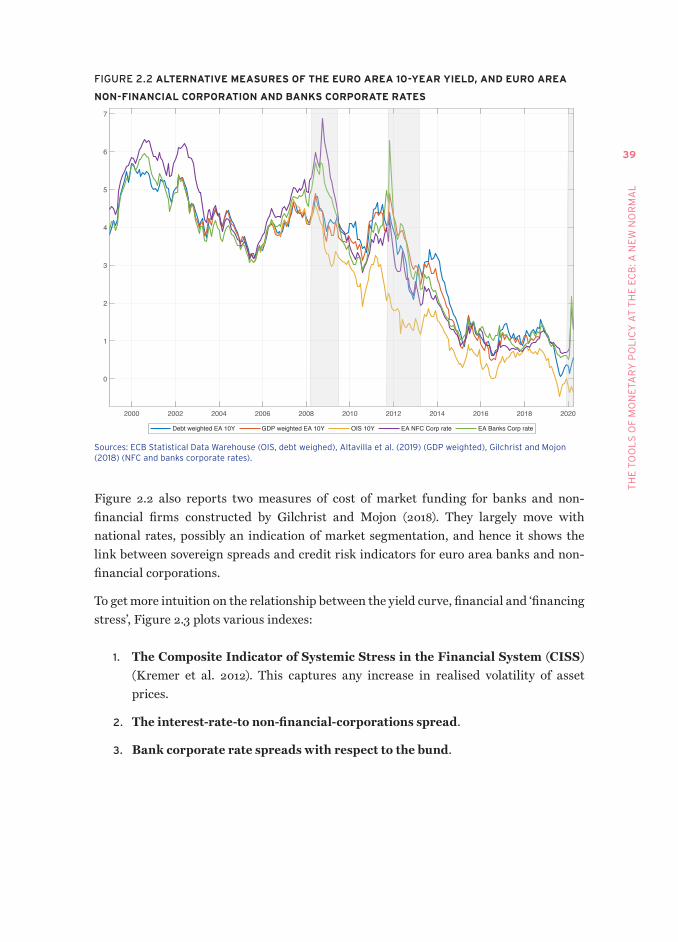
39
TH
E T
OO
LS
OF
MO
NE
TAR
y P
OL
ICy
AT
TH
E E
CB
: A N
EW
NO
RM
AL
FIGURE 2.2 ALTERNATIvE MEASURES OF THE EURO AREA 10-YEAR YIELD, AND EURO AREA
NON-FINANCIAL CORPORATION AND BANKS CORPORATE RATES
2000 2002 2004 2006 2008 2010 2012 2014 2016 2018 2020
0
1
2
3
4
5
6
7
Debt weighted EA 10Y GDP weighted EA 10Y OIS 10Y EA NFC Corp rate EA Banks Corp rate
Sources: ECB Statistical Data Warehouse (OIS, debt weighed), Altavilla et al. (2019) (GDP weighted), Gilchrist and Mojon (2018) (NFC and banks corporate rates).
Figure 2.2 also reports two measures of cost of market funding for banks and non-financial firms constructed by Gilchrist and Mojon (2018). They largely move with national rates, possibly an indication of market segmentation, and hence it shows the link between sovereign spreads and credit risk indicators for euro area banks and non-financial corporations.
To get more intuition on the relationship between the yield curve, financial and ‘financing stress’, Figure 2.3 plots various indexes:
1. The Composite Indicator of Systemic Stress in the Financial System (CISS) (Kremer et al. 2012). This captures any increase in realised volatility of asset prices.
2. The interest-rate-to non-financial-corporations spread.
3. Bank corporate rate spreads with respect to the bund.
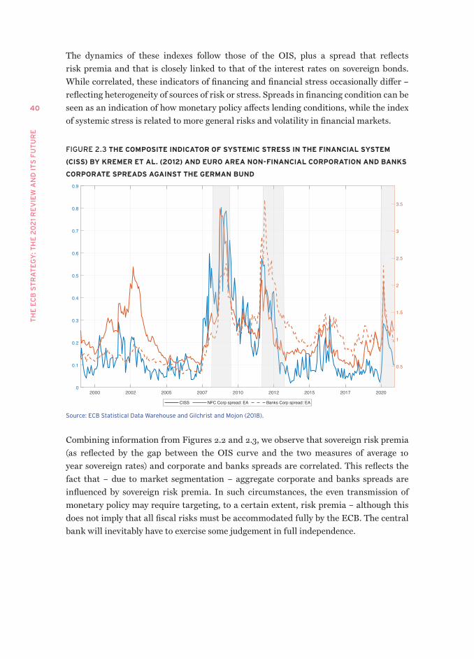
TH
E E
CB
ST
RA
TE
GY
: TH
E 2
02
1 R
EV
IEW
AN
D I
TS
FU
TU
RE
40
The dynamics of these indexes follow those of the OIS, plus a spread that reflects risk premia and that is closely linked to that of the interest rates on sovereign bonds. While correlated, these indicators of financing and financial stress occasionally differ – reflecting heterogeneity of sources of risk or stress. Spreads in financing condition can be seen as an indication of how monetary policy affects lending conditions, while the index of systemic stress is related to more general risks and volatility in financial markets.
FIGURE 2.3 THE COMPOSITE INDICATOR OF SYSTEMIC STRESS IN THE FINANCIAL SYSTEM
(CISS) BY KREMER ET AL. (2012) AND EURO AREA NON-FINANCIAL CORPORATION AND BANKS
CORPORATE SPREADS AGAINST THE GERMAN BUND
2000 2002 2005 2007 2010 2012 2015 2017 20200
0.1
0.2
0.3
0.4
0.5
0.6
0.7
0.8
0.9
0.5
1
1.5
2
2.5
3
3.5
CISS NFC Corp spread: EA Banks Corp spread: EA
Source: ECB Statistical Data Warehouse and Gilchrist and Mojon (2018).
Combining information from Figures 2.2 and 2.3, we observe that sovereign risk premia (as reflected by the gap between the OIS curve and the two measures of average 10 year sovereign rates) and corporate and banks spreads are correlated. This reflects the fact that ‒ due to market segmentation ‒ aggregate corporate and banks spreads are influenced by sovereign risk premia. In such circumstances, the even transmission of monetary policy may require targeting, to a certain extent, risk premia – although this does not imply that all fiscal risks must be accommodated fully by the ECB. The central bank will inevitably have to exercise some judgement in full independence.
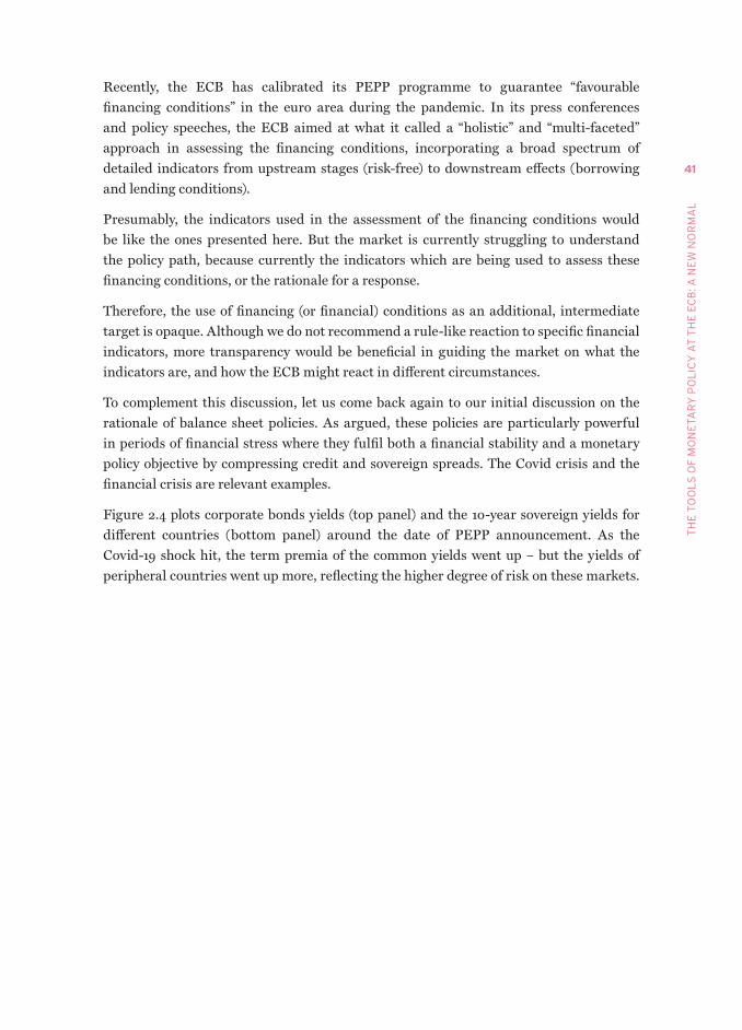
41
TH
E T
OO
LS
OF
MO
NE
TAR
y P
OL
ICy
AT
TH
E E
CB
: A N
EW
NO
RM
AL
Recently, the ECB has calibrated its PEPP programme to guarantee “favourable financing conditions” in the euro area during the pandemic. In its press conferences and policy speeches, the ECB aimed at what it called a “holistic” and “multi-faceted” approach in assessing the financing conditions, incorporating a broad spectrum of detailed indicators from upstream stages (risk-free) to downstream effects (borrowing and lending conditions).
Presumably, the indicators used in the assessment of the financing conditions would be like the ones presented here. But the market is currently struggling to understand the policy path, because currently the indicators which are being used to assess these financing conditions, or the rationale for a response.
Therefore, the use of financing (or financial) conditions as an additional, intermediate target is opaque. Although we do not recommend a rule-like reaction to specific financial indicators, more transparency would be beneficial in guiding the market on what the indicators are, and how the ECB might react in different circumstances.
To complement this discussion, let us come back again to our initial discussion on the rationale of balance sheet policies. As argued, these policies are particularly powerful in periods of financial stress where they fulfil both a financial stability and a monetary policy objective by compressing credit and sovereign spreads. The Covid crisis and the financial crisis are relevant examples.
Figure 2.4 plots corporate bonds yields (top panel) and the 10-year sovereign yields for different countries (bottom panel) around the date of PEPP announcement. As the Covid-19 shock hit, the term premia of the common yields went up – but the yields of peripheral countries went up more, reflecting the higher degree of risk on these markets.
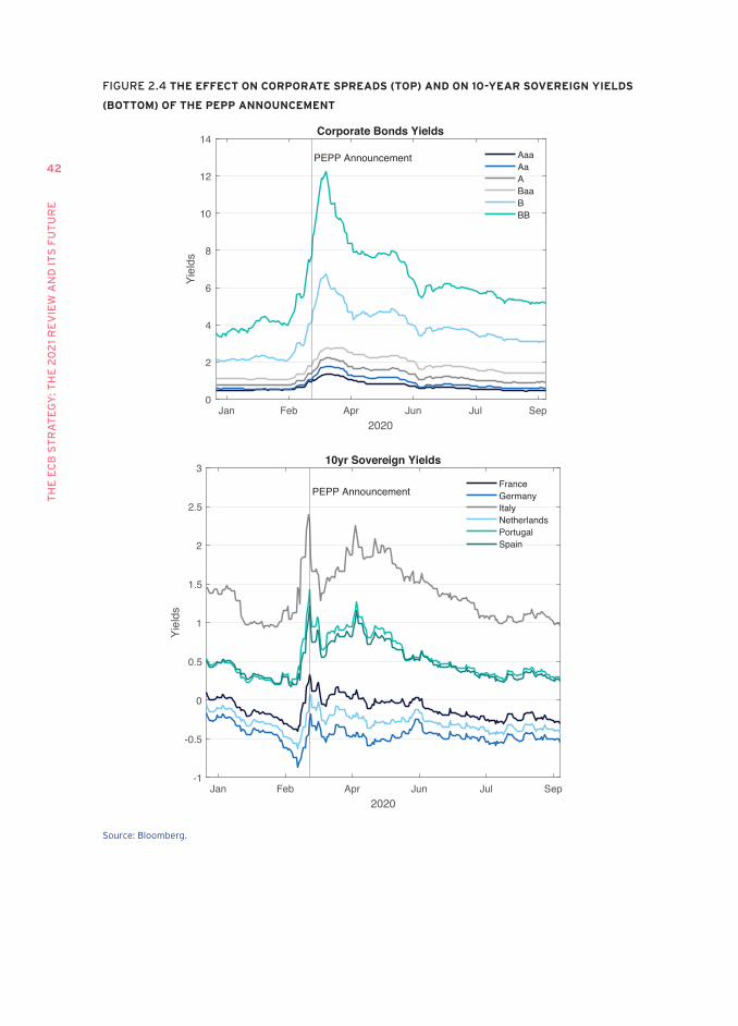
TH
E E
CB
ST
RA
TE
GY
: TH
E 2
02
1 R
EV
IEW
AN
D I
TS
FU
TU
RE
42
FIGURE 2.4 THE EFFECT ON CORPORATE SPREADS (TOP) AND ON 10-YEAR SOvEREIGN YIELDS
(BOTTOM) OF THE PEPP ANNOUNCEMENT
Jan Feb Apr Jun Jul Sep2020
0
2
4
6
8
10
12
14
Yiel
ds
Corporate Bonds Yields
PEPP Announcement AaaAaABaaBBB
Jan Feb Apr Jun Jul Sep2020
-1
-0.5
0
0.5
1
1.5
2
2.5
3
Yiel
ds
10yr Sovereign Yields
PEPP AnnouncementFranceGermanyItalyNetherlandsPortugalSpain
Source: Bloomberg.
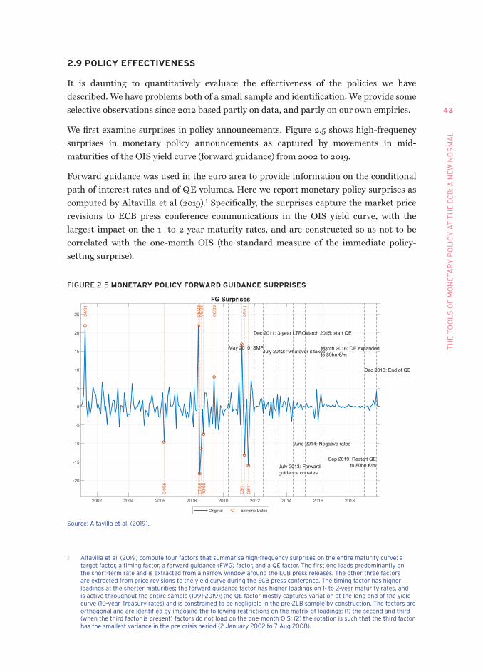
43
TH
E T
OO
LS
OF
MO
NE
TAR
y P
OL
ICy
AT
TH
E E
CB
: A N
EW
NO
RM
AL
2.9 POLICY EFFECTIvENESS
It is daunting to quantitatively evaluate the effectiveness of the policies we have described. We have problems both of a small sample and identification. We provide some selective observations since 2012 based partly on data, and partly on our own empirics.
We first examine surprises in policy announcements. Figure 2.5 shows high-frequency surprises in monetary policy announcements as captured by movements in mid-maturities of the OIS yield curve (forward guidance) from 2002 to 2019.
Forward guidance was used in the euro area to provide information on the conditional path of interest rates and of QE volumes. Here we report monetary policy surprises as computed by Altavilla et al (2019).1 Specifically, the surprises capture the market price revisions to ECB press conference communications in the OIS yield curve, with the largest impact on the 1- to 2-year maturity rates, and are constructed so as not to be correlated with the one-month OIS (the standard measure of the immediate policy-setting surprise).
FIGURE 2.5 MONETARY POLICY FORWARD GUIDANCE SURPRISES
2002 2004 2006 2008 2010 2012 2014 2016 2018
-20
-15
-10
-5
0
5
10
15
20
25
FG Surprises
May 2010: SMP
Dec 2011: 3-year LTRO
July 2012: "whatever it takes"
July 2013: Forwardguidance on rates
June 2014: Negative rates
March 2015: start QE
March 2016: QE expanded
Dec 2018: End of QE
Sep 2019: Restart QE
04/0
1
06/0
808
/08
06/0
9
05/1
1
04/0
6
07/0
810
/08
03/1
108
/11
Original Extreme Dates
Source: Altavilla et al. (2019).
1 Altavilla et al. (2019) compute four factors that summarise high-frequency surprises on the entire maturity curve: a target factor, a timing factor, a forward guidance (FWG) factor, and a QE factor. The first one loads predominantly on the short-term rate and is extracted from a narrow window around the ECB press releases. The other three factors are extracted from price revisions to the yield curve during the ECB press conference. The timing factor has higher loadings at the shorter maturities; the forward guidance factor has higher loadings on 1- to 2-year maturity rates, and is active throughout the entire sample (1991-2019); the QE factor mostly captures variation at the long end of the yield curve (10-year Treasury rates) and is constrained to be negligible in the pre-ZLB sample by construction. The factors are orthogonal and are identified by imposing the following restrictions on the matrix of loadings: (1) the second and third (when the third factor is present) factors do not load on the one-month OIS; (2) the rotation is such that the third factor has the smallest variance in the pre-crisis period (2 january 2002 to 7 Aug 2008).
TH
E E
CB
ST
RA
TE
GY
: TH
E 2
02
1 R
EV
IEW
AN
D I
TS
FU
TU
RE
44
The chart shows that the crisis period (2008-2012) is characterised by relatively high volatility, indicating that the market was often surprised by the medium-term ECB communication. After July 2012 (when the “whatever it takes” speech was delivered) and especially after July 2013, when forward guidance was implemented as a policy, volatility declines further with a decisive decline after late 2014, when QE is implemented. The chart suggests that indeed the definition of the new operational framework, and in particular asset purchases, helped markets to interpret ECB communication.
Delayed QE was probably part of the market’s confusion about ECB policy. Recall that before the implementation of the asset purchase programme and since 2012, the Eurosystem balance sheet was shrinking (Figure 2.1) as a consequence of bank deleveraging and increased preference for safety that had resulted from the debt crisis. Around the same time, long-term interest rates started declining persistently (Figure 2.6).
FIGURE 2.6 GERMANY, FRANCE, ITALY, SPAIN AND THE OUTSTANDING DEBT-WEIGHTED EURO
AREA 10-YEAR BOND YIELDS
-2
-1
0
1
2
3
4
5
6
7
8
Jan-06 Jan-07 Jan-08 Jan-09 Jan-10 Jan-11 Jan-12 Jan-13 Jan-14 Jan-15 Jan-16 Jan-17 Jan-18 Jan-19 Jan-20
YoY %
10-year government bond yield
Euro area Germany France Italy Spain
July 2012: "whatever it takes"
July 2013: Forward Guidance on rates
June 2014: negative rates
March 2015: start QE
March 2016: QE expanded to 80bn€/m
Dec 2018: end of QE
Sep 2019: restart QEDec 2011: 3-year LTRO
May 2010: SMP
Apr & Jul 2011: increases
Jul 2008: increaseNov 2011: decrease
Oct, Nov & Dec 2008: decreases
Source: Bloomberg.
We can conjecture that declining growth expectations and flight to safety drove the natural interest rate downwards while the effective financing conditions, caused by inadequate policy and delayed implementation of QE, did not accommodate that change. This caused long-term inflation expectations to trend down. While inflation expectations also weakened in the US, the decline in the euro area was sharper. Indeed, a gap between inflation expectations in the US and the euro area emerged in that period and has persisted since (see the Appendix).
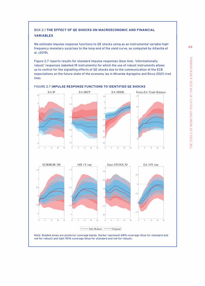
45
TH
E T
OO
LS
OF
MO
NE
TAR
y P
OL
ICy
AT
TH
E E
CB
: A N
EW
NO
RM
AL
BOX 2.1 THE EFFECT OF QE SHOCKS ON MACROECONOMIC AND FINANCIAL
vARIABLES
We estimate impulse response functions to QE shocks using as an instrumental variable high-
frequency monetary surprises to the long-end of the yield curve, as computed by Altavilla et
al. (2019).
Figure 2.7 reports results for standard impulse responses (blue line), ‘informationally
robust’ responses (labelled IR instruments) for which the use of robust instruments allows
us to control for the signalling effects of QE shocks due to the communication of the ECB
expectations on the future state of the economy (as in Miranda-Agrippino and Ricco 2021) (red
line).
FIGURE 2.7 IMPULSE RESPONSE FUNCTIONS TO IDENTIFIED QE SHOCKS
0 6 12 18 24
-4
-2
0
2
4
6
8EA IP
Info Robust Original
0 6 12 18 24
-1.5
-1
-0.5
0
0.5
1
1.5
2
EA HICP
0 6 12 18 24
-30
-25
-20
-15
-10
-5
0
5
10
EA NEER
0 6 12 18 24
-5
0
5
10
15
Extra-EA Trade Balance
0 6 12 18 24
-1
-0.5
0
0.5
1
1.5
EURIBOR 3M
0 6 12 18 24
-1
-0.5
0
0.5
1
1.5
OIS 1Y rate
0 6 12 18 24
-20
-10
0
10
20
30
Euro STOXX 50
0 6 12 18 24
-1.5
-1
-0.5
0
0.5
EA 10Y rate
Note: Shaded areas are posterior coverage bands. Darker represent 68% coverage (blue for standard and red for robust) and light 90% coverage (blue for standard and red for robust).
TH
E E
CB
ST
RA
TE
GY
: TH
E 2
02
1 R
EV
IEW
AN
D I
TS
FU
TU
RE
46
This conjecture would benefit from the support of quantitative analysis of the effect of QE on inflation. As we said, lack of a sufficiently long sample (asset purchases were implemented only in early 2015) and the general difficulty to identify exogenous policy changes makes it problematic to come to a solid conclusion. Nonetheless, we report new results from work in progress by Reichlin et al. (2021c) in Box 2.1.
They show the effect of a shock which can be essentially interpreted as a shock to the long end of the 10-year risk-free OIS curve. In our taxonomy, this is the ‘active’ type of balance sheet policy, which targets the long-term rate when the scope of easing via a short-term rate cut is exhausted because of the effective lower bound. Thus defined, this shock is meant to affect the term premium of the risk-free curve rather than sovereign spreads.
Results indicate that a shock on the risk-free rate has a significant negative effect on the debt-weighted 10-year yield (EA 10-year rate), the term spread, and the effective nominal exchange rate (EA NEER). Macroeconomic effects on inflation and output are more uncertain (see also the discussion in Chapter 1).
A QE shock that compresses the debt-weighted EA 10-year yield of 100 basis points induces at peak, respectively, a 4% increase in industrial production and a 0.2% increase in prices.2 These estimates are broadly in line with previous research (see Hartmann and Smets 2018 and Dell’Ariccia et al. 2018 for a literature review and a comparison with previous estimates). Finally, as to be expected, we estimate a positive effect on the stock market.
To summarise: since 2012, notwithstanding the strong effect on sovereign spreads and risk premia following Draghi’s speech, inflation expectations started trending down and market surprises related to ECB announcements remained volatile until the asset purchase programme was announced in late 2014, and implemented in 2015.
This suggests that the progressive clarification of the operational framework and the implementation of the entire toolbox, including QE, stabilised market expectations. It also suggests that delays in implementing all potentially available tools was costly. There is also evidence that QE had some impact – although highly uncertain – on inflation and output, and this is associated with a persistent decline in the long-term euro area average yield curve and the exchange rate. These considerations support the decision by the ECB (outlined in the strategy review) to include in its regular operational framework all tools developed in the last 13 years, including asset purchases.
2 Reichlin et al. (2021a) show empirically that the muted effect on inflation of QE shocks is explained in part by the fiscal policy response.
47
TH
E T
OO
LS
OF
MO
NE
TAR
y P
OL
ICy
AT
TH
E E
CB
: A N
EW
NO
RM
AL
2.10 CONCLUSION
The ECB’s mission review of 2020-21 has affirmed a new normal for its operating procedures. Much of it is simply a normalisation of the policies of the last 10 years. The ECB should now shake off the habit of calling these monetary policy operations ‘extraordinary’ and ‘exceptional’.
The review remains vague on how to translate such a complex set of policies into an operational target. We recommend it communicates policies in terms of their effect on interest rates rather than quantities. An objective in terms of the risk-free yield curve should be part of the regular communication.
We also recognise the need, in segmented financial markets and in periods of financial stress, for monetary policy and financial stability to target risk premia. Transparent communication will be the key condition for effectiveness and credibility of these policies.

49
CHAPTER 3
Fiscal and monetary interactions
SUMMARY RECOMMENDATIONS
• Inflation is jointly determined by the stance of fiscal and monetary policy. Understanding and correctly assessing fiscal-monetary interactions in the euro area has become a more pressing issue in the recent past and will be even more pressing in the near future. The ECB’s mission review partially acknowledges this, but should discuss it further because it is important to clarify the fiscal footprint of its actions, the fiscal support it has, and the fiscal activism it must interact with.
• With a large balance sheet characterised by a duration mismatch between assets and liabilities, the ECB is subject to the risk of net income fluctuations that in extreme (and very rare) cases could lead to significant losses. To avoid this jeopardising the goal of price stability, it is important to clarify how the Eurosystem would rebuild its net worth if there are large losses. We propose clearer rules for callable capital by the fiscal authorities as a transparent way to do so.
• The risk-sharing arrangements within the EMU are ambiguous and unclear. We discuss the present system and possible alternative options. Although this is beyond the scope of the strategy review, the topic is important. It should be on the agenda of future fiscal reviews in the EU, and the ECB should, maintaining its independence, contribute to those discussions by alerting political authorities to the consequences that different options have for its balance sheet and for preserving the independence of monetary policy.
• Given the need for a regular analysis and oversight of fiscal-monetary interactions with a union-wide perspective, we suggest establishing a board based on the model of the European Systemic Risk Board. Its goal would be to identify incongruences between monetary and fiscal policy, and to support the independent decisions of the ECB and the fiscal authorities. We recognise, however, that the decision of whether to establish such board and the design of its governance should not be the ECB’s responsibility.
TH
E E
CB
ST
RA
TE
GY
: TH
E 2
02
1 R
EV
IEW
AN
D I
TS
FU
TU
RE
50
INTRODUCTION
It is an obvious (but often neglected) principle of economics that macroeconomic outcomes, particularly inflation, are affected jointly by monetary and fiscal policy. No theory of inflation is well specified unless it explains how monetary and fiscal policy respond to each other, either directly or indirectly, through real and financial activity.3 At the same time, the logic of general equilibrium is that all outcomes depend on all policies and all shocks. Acknowledging that there are interactions between monetary and fiscal policy, and that the ECB does not live in a cloud floating over the fiscal authorities in the euro area, does not amount to questioning the independence of the institution.
Theory and experience support the delegation of monetary policy to an independent authority that focuses on inflation as its main target. Distributional considerations are paramount in almost all fiscal policies, but they are less pressing (though not irrelevant) in monetary policy. Thus, there are different interactions between economic and political considerations for the two types of policy. Monetary policy also suffers from biases and time inconsistencies when it is set jointly with fiscal policy. Independent inflation-targeting central banks have become the norm across the globe over the past 30 years, and this has resulted in low and stable inflation with no noticeable loss in real outcomes (Alesina and Stella 2010).
The delegation of a part of policy to a narrow mandate does not deny the interactions between different policies, nor does it ignore the fact that ultimately the goal is to advance the social welfare of the citizens of the euro area. Instead, delegation is a way to formalise how many of these interactions should take place, which rules should govern them, what the priorities are, and which limits they are subject to. The focus on inflation for the central bank comes from the tight link between monetary policy and the price level, and it serves to clarify how policy should balance price stability against other desirable outcomes when trade-offs emerge.
If the discussion of fiscal-monetary interactions is one that is central to the mandate and mission of every central bank, it is particularly important in the euro area. In the case of the ECB, the need to lay out these boundaries and trade-offs is amplified by the existence of one monetary authority that interacts with many fiscal authorities. The fact that there is no fiscal union does not compromise the existence or survival of the monetary union, but it poses specific challenges and requires different principles for these interactions. The Maastricht Treaty laid out the founding principles of this interaction but, as with
3 See Castillo-Martinez and Reis (2019) on the theory behind the determination of inflation, Leeper and Leith (2016) and Cochrane (2019, 2020) for fiscal-monetary interactions in the context of the fiscal theory of the price level, and Reichlin et al. (2021a) for an empirical framework to evaluate these interactions in the monetary union.
51
FIS
CA
L A
ND
MO
NE
TAR
y IN
TE
RA
CT
ION
S
any foundational treaty, the way it is interpreted must evolve. The review could have been clearer in how the interpretation of the Treaty has evolved under the changing economic circumstances and given the progress in economic knowledge since the Treaty was signed.
This chapter discusses what might guide the separation of monetary and fiscal policy in the euro area in the next few years. We examine its history, going back to Maastricht, and how the early interpretations of the Treaty reflected both the economic principles that dominated during the first decade of the ECB and the circumstances of the economy during that time.
We discuss what the pressing interactions between monetary and fiscal policy will likely be in the near future, the financial risks facing the central bank, and how the circumstances of the euro area mean that these risks come with implications about fiscal risk sharing. Sovereign default risk is a particular form of risk in the euro area that poses special challenges. We conclude with a critical diagnosis of the current status quo of ‘constructive ambiguity’ with respect to many of these risks. We discuss different solutions, while noting that any one solution has fiscal consequences and hence that the ECB cannot legitimately decide on it by itself. This leads to a discussion of how future institutional reforms of the euro area should consider monetary and fiscal interactions.
3.1 THE MAASTRICHT CONTExT, PRINCIPLES, AND LEGACY
In the late 1980s, academic research focused on understanding how politicians would be tempted to use monetary policy such that inflation would deviate from expectations. This could be to surprise bondholders and lower the real value of the nominal public debt, or to surprise wage and price setters into accepting lower real wages and relative prices for their work and goods and, in doing so, increase output and employment. Theories and empirical work showed that this temptation on average led to inferior outcomes, with average inflation that was forever higher because inflation expectations remained high. A solution to this time-inconsistency problem was to take discretion over monetary policy away from politicians and place it into the hands of independent technocrats with a clear mandate to keep inflation steady and predictable.
The historical experience had been marked by the high inflation of the 1970s and the 1980s recessions associated with bringing inflation down. Several countries in Europe in the decade before the Maastricht Treaty had struggled with balancing public accounts, resulting in fiscal crises and persistently high interest rates on government borrowing. These fiscal troubles were partly responsible for volatile inflation and exchange rates.
In this context, the Maastricht Treaty was designed and, at first, interpreted to ensure a strict separation between monetary and fiscal policy. The ECB’s decision-making procedures and the appointments to its governing council were protected from undue political influence by the Treaty. Unlike many other central banks, the ECB’s monetary
TH
E E
CB
ST
RA
TE
GY
: TH
E 2
02
1 R
EV
IEW
AN
D I
TS
FU
TU
RE
52
interventions initially did not include outright purchases of government securities, instead favouring a refinancing programme. Monetary financing of fiscal deficits was explicitly forbidden, even if is hard to pin down what this expression means in a world where almost every central bank action has some spillovers to the government accounts. It is probably best interpreted as a statement that infers intent from central bank actions: lowering interest rates with an eye to bringing inflation up and closer to the objective is admitted, while lowering interest rates with the sole purpose to alleviate the fiscal financing burden is not. The Treaty focuses the ECB on controlling inflation and excludes the temptation for it to develop, or be pressured into, fiscal concerns.
For the fiscal position of the ECB itself, the Treaty established the financial independence of the Eurosystem by requiring that any national central bank (NCB) had to be adequately capitalised. Starting from a positive net worth, it gave the ECB some freedom to provision its net income before distributing it to the NCBs. Each of the NCBs then has its own rules on distributing income to their fiscal authorities. This reflected a view that a minimalist central bank facing an ever-increasing demand for banknotes would generate a steady positive net income, so that no fiscal backing or transfers from the fiscal authorities would ever be needed for the actions of monetary policy.
The Maastricht Treaty also reflected a belief that, in an asymmetric federation with a single monetary policy authority and many fiscal authorities, macroeconomic stability could be ensured by a combination of a credible and independent central bank targeting price stability, plus centrally mandated fiscal rules setting public deficit and public debt limits at the national level. Parallel to the ECB, there were fiscal rules for the levels of the public deficit and the public debt, as well as an explicit commitment to have no bailouts between nations. These fiscal rules were effectively a commitment that each country individually would follow a passive fiscal policy, raising its primary surplus by more than enough to offset the increased interest payments when real debt grew. The Maastricht Treaty enforced this fiscal adjustment in the short and medium run, not just in the long run, leaving the ECB and monetary policy with active control over inflation.
In sum, the Treaty clearly separated fiscal and monetary policy and gave a large degree of autonomy to the ECB. The Treaty can be thought of as enforcing an equilibrium in which fiscal authorities would absorb shocks of ECB actions on public debt markets, would fiscally back any fluctuations in the ECB’s net income, and would be fiscally passive when it came to inflation control. It was a coordination device to avoid a strategic game between several fiscal authorities and one monetary authority. At the same time, the interpretation of these principles in the first decade of the euro was very strict: the ECB should have a minimal fiscal footprint, did not require any explicit fiscal backing, and could control inflation as fiscal policy was forced by rule to be passive.
53
FIS
CA
L A
ND
MO
NE
TAR
y IN
TE
RA
CT
ION
S
3.2 MONETARY FISCAL INTERACTIONS IN THE EURO AREA TODAY
The problem with such a rigid interpretation of the separation between monetary and fiscal policies in the Treaty is that it was not possible under all circumstances. It worked for the first decade of the euro, but events soon showed it was not sustainable for longer periods.
3.2.1 Fiscal footprint
The fiscal footprint of central bank policies is not constrained solely by whether the central bank purchases government bonds outright or not. There are many other channels. Monetary policy, whether conventional or unconventional, affects yield curves in the euro area. In doing so, the central bank influences the effective cost of servicing the debt for every national fiscal authority, and this effect can be quite different across countries depending on the size and position of their public debt. If expected inflation or actual inflation move, these also affect the expected inflation and risk premia that a euro area government must pay, as well as the real revaluations of its nominal debt burden. More directly, though minor on a macroeconomic scale, the net income of the central bank that is distributed as dividends directly affects the primary surplus. Indirectly, but more substantial, by influencing lending and real activity, the central bank will affect the tax base and thus the primary deficits of the government. All these channels are potentially large.4
In the other direction, purchasing government bonds by itself does not lead to a fiscal footprint. If the central bank directly purchases government bonds in exchange for deposits at the central bank, this may well be fiscally neutral, especially when nominal interest rates are near zero. If the interest rate that the central bank pays to its depositors is approximately the same as the yield on the government bond that it bought, then the expenses and revenues of both the central bank, and the fiscal authority, are approximately unchanged (Wallace 1981, Benigno and Nisticò 2020).
In terms of experience, as the ECB has embraced QE and has actively intervened in government debt markets (as already discussed in the previous chapter), the interactions between monetary and fiscal policy have increased. As the ECB has started going long in its interest-rate management, the effects of policy on long-term financing costs have become more obvious. As the balance sheet has grown, the potential for larger net income fluctuations and so dividends has grown as well.
4 On the fiscal footprint of monetary policies, see Reis (2019). On the fiscal effect of monetary policy, see Reichlin et al. (2021a).
TH
E E
CB
ST
RA
TE
GY
: TH
E 2
02
1 R
EV
IEW
AN
D I
TS
FU
TU
RE
54
Both theory and circumstances imply that an interpretation of what “no monetary financing of the public debt” means must be clarified. This clarification is also linked to the clarification of the operational target formulated in terms of the euro area yield curve, as discussed in Chapter 2.
3.2.2 Fiscal support
Two important developments have required a reinterpretation of the Maastricht dispositions. First, the increased digitalisation of payment systems has reduced the reliance on banknotes issued by the central bank. Therefore, the net income that follows from printing these banknotes (seigniorage) may become smaller in years to come. If the ECB issues digital central bank money in the form of reserves or a digital euro, new forms of seigniorage may arise. The combined effect of these systemic changes means we don’t know for certain what the medium-term net income of the central bank will be.
Second, as monetary policy has led to an increase in the size of the balance sheet of the central bank (Chapter 2), this has come with a mismatch in duration between the maturity of the assets and the liabilities of the ECB. As it issues short-term deposits remunerated at a short-term interest rate but earns long-term interest rates on the government bonds on its balance sheet, changes in the slope of the yield curve create fluctuations in the net income of the central bank. This inevitably leads to periods in which the ECB may make losses, and in some (rare) occasions when there is a sharp unexpected movement in inflation and on the stance of monetary policy, these losses could be large and exceed previous provisions (Hall and Reis 2015, Bhattarai et al. 2021).
If it is so, then it is conceivable that the equity of some national central banks could fall, making a recapitalisation necessary. But, while the Maastricht Treaty requires national central banks to be adequately capitalised, it does not compel national fiscal authorities to provide these recapitalisations. The fiscal support of the central bank needs clarification.
3.2.3 Fiscal activism
Finally, fiscal policy has direct impacts on inflation and can hinder the attainment of the fiscal target, even in a regime with ‘passive’ fiscal policy. The stance of fiscal policy affects the level of real activity, as well as the equilibrium real interest rate that equates savings and investment. Structural policies, for instance, affect the growth potential of economies and thereby influence equilibrium real rates. These, in turn, have a direct effect on the inflation pressures to which the monetary policy must respond.
Circumstances have made the effects of fiscal policy on inflation more pressing. The decline of equilibrium real interest rates in the last 20 years has made it more likely that the ECB finds itself against an effective lower bound on short-term interest rates. In these circumstances, fiscal policy is particularly impactful on activity and inflation. When there are large supply shocks – pandemics, for example, or climate emergencies – this
55
FIS
CA
L A
ND
MO
NE
TAR
y IN
TE
RA
CT
ION
S
spillover of fiscal policy to inflation can be especially large. When it comes to stabilising real activity, fiscal policy can be more targeted and effective than the blunt instrument of monetary policy. When it comes to inflation, large supply shocks create a steep trade-off between inflation and real activity, which fiscal policy can greatly ameliorate (Bartsch et al. 2020).
All combined, the interactions between monetary and fiscal policies have increased in the last decade. This necessitates a reinterpretation of the Maastricht Treaty that protects the independence of monetary policy by restating boundaries and procedures. It has become increasingly difficult to ignore the fiscal footprint of monetary policy, to neglect the fiscal support that monetary policy needs to stay financially independent, or to deny the difficulties that fiscal activism may pose for achieving the inflation objective. Future mission reviews will increasingly have to clarify whether, and to what extent, the fiscal footprints of monetary policy decisions should influence monetary policy choices – and how fiscal support and fiscal activism affect what monetary policy can achieve.
3.3 DIRECT FISCAL RISKS FOR THE CENTRAL BANK, AND THE PRINCIPLE OF
ECB FISCAL SUPPORT
An increase in the size of the central bank’s balance sheet by itself does not necessarily increase the direct financial risks for the central bank. Exchanging deposits at the central bank for short-term government bonds has no impact on the net income of the central bank, insofar as the interest rates of the asset and the liability are approximately the same (and as long as the bonds do not default, a discussion of which we defer to Section 3.5). In the last few years, with interest rates for both at zero, the net impact has been zero and so is the gross impact.
When the central bank instead buys long-term government bonds with the resources from its zero-duration deposits, it becomes exposed to duration risk. A sudden increase in interest rates, and so a fall in the price of long-term bonds, will cause a capital loss for the central bank. If the central bank refuses to book these losses to market and holds the bonds to maturity, then it will pay higher interest rates on its deposits while collecting the previously-set low coupons on the long-term bonds, making a loss year after year.
From the perspective of the consolidated government accounts – central bank and treasury – this risk may cancel out. Any losses from a fall in the value of the long-term bonds to the central bank are gains to the treasury and vice versa. However, the financial independence of the central bank implies that there is no such automatic consolidation. The limits to the flow of resources between the central bank and the treasury are both what gives it its independence, but also what limits its fiscal backing by the government (and, in the extreme, what creates the possibility of an insolvent central bank). When the
TH
E E
CB
ST
RA
TE
GY
: TH
E 2
02
1 R
EV
IEW
AN
D I
TS
FU
TU
RE
56
ECB makes gains, the rules that force it to distribute its net income to the NCBs, and from these to the national treasuries, ensure that this consolidation happens. When it makes losses, though, the Treaty does not encode how the fiscal authorities will proceed to transfer their gains back to the central bank.
By itself, the ECB does not have the fiscal capacity to absorb significant losses permanently; its paid-up capital is too small. The revenue from the seignorage that results from printing banknotes is significant, but governments expect to receive its flow as dividends in the future. Once it is exhausted, then one of two outcomes is likely:
• The central bank becomes insolvent. This is an unlikely but possible event and should be interpreted as a situation in which banks realise that their reserves are not backed by assets or future flows of seignorage and try to switch into real assets, which causes inflation.
• The central bank voluntarily pursues a higher inflation target. This would increase its seignorage revenue, by collecting more of the ‘inflation tax’.
Either way, having the ECB exposed to possible losses without having secured a certain fiscal support is incompatible with the Treaty’s stated primacy of price stability. Simply put, fiscal gains and losses cannot stay in the monetary authority, they must be distributed or recovered from the fiscal authorities to be consistent with an inflation target (Hall and Reis 2015, Del Negro and Sims 2015, Corsetti and Dedola 2016).
Currently, the ECB has the power to retain earnings as provisions that eventually get converted into capital, but this provides only a limited buffer with which to deal with potential losses. One possible solution to this problem would be for the Eurosystem to have callable capital. In case of unexpected large losses that arise in the conduct of monetary policy, both the ECB and the NCBs would have to right to require a recapitalisation. This would be under a set of clear and strict rules that ensure the ECB behaves prudently in managing its portfolio risk, and that exclude sovereign default as a trigger.
Because, as we explained, in most cases the losses of the central bank are matched by gains to the treasuries, these would not put undue stress on public accounts. And the cases in which the capital would have to be called are quite rare. It is important that these rules are in place, so there is no question about the fiscal support of the central bank in any circumstance, including very rare ones. This will avoid possibly self-reinforcing inflation episodes, where fears about inflation create the losses in the central bank’s portfolio that feed expectations of inflation resulting from those losses.
57
FIS
CA
L A
ND
MO
NE
TAR
y IN
TE
RA
CT
ION
S
The principle of ECB fiscal support is, therefore, of crucial importance. The Treaty recognised this when it stated the obligation of national governments to keep the net equity of NCBs positive. Currently, it is not well defined how this obligation is to be enforced when the Eurosystem as a whole has significantly negative equity that might exceed the present value of future seignorage. Callable capital guided by clear criteria established ex ante would be a way to make this clear and watertight, as it should be.
3.4 BOND ISSUANCE AND BOND PURCHASE PROGRAMMES
When the central bank buys long-term bonds in secondary markets, this can affect long-term yields by affecting the net supply of these bonds to the private sector, as discussed in Chapter 2. However, the ultimate effectiveness of this policy depends on how the treasury responds in its issuance of new bonds.
At one extreme, if the maturity of issuance is unchanged, then by taking long-term bonds from private hands and replacing them with zero-duration reserves, the central bank is reducing the maturity of the government liabilities in the hands of the private sector. This changes the risk profile for the government accounts.
At the other extreme, if the treasury changes issuance to exactly match the purchases of the central bank, then there would be no change in the interest-rate exposure of the private sector, so the effects of QE on yields would likely become much smaller. In between these two extremes, some coordination between the actions of the central bank and those of the treasury is inevitably required when it comes to affecting long-term government bond yields (Greenwood et al. 2015).
In Chapter 2, we suggested that the ECB should express its policy actions increasingly in reference to the common yield curve of the euro area (although we do not advocate yield curve control). This form of communication could help avoid some of the more extreme mis-coordination between bond purchases and bond issuances. By stating its policies in this way, the ECB might gain a first-mover advantage in the interaction with the treasury, while avoiding fiscal dominance. Communicating that objective, and conducting policy in coherence with it, would also be the basis for distinguishing between purchases for monetary policy purposes as opposed to fiscal policy.
A harder problem is that the ECB has suffered the consequences of not having a euro-area-wide safe asset. Without this, in time of crisis, there is flight of safety across regions as opposed to asset classes leading to large current account reversals that threaten macroeconomic stability. Without a euro area-wide safe asset, the diabolic loop linking the health of banks to their national sovereign through the holding of national banks cannot be solved. Without a euro area-wide safe asset, the ECB can only approximate what would be region-neutral QE and evaluate what might be a euro area-wide yield curve (Chapter 2).
TH
E E
CB
ST
RA
TE
GY
: TH
E 2
02
1 R
EV
IEW
AN
D I
TS
FU
TU
RE
58
3.5 THE CHALLENGE OF RISK SHARING AND THE UNSUSTAINABILITY OF
‘CONSTRUCTIvE AMBIGUITY’
With segmented fiscal authorities and the absence of a euro area-wide safe bond, there are few actions, monetary or otherwise, that do not lead to some transfers across regions, and so we cannot avoid discussing how risks should be shared among the members of the Eurosystem. While it is not the ECB’s role to decide on the overall extent of risk sharing, it cannot ignore the transfers that its actions may cause. More concretely, it cannot avoid deciding how much risk sharing it will allow between the NCBs.
Currently, 80% of the assets purchased under the APP and PEPP programmes are held by the NCBs, with each holding the government bonds of their nation. Consequently, potential losses related to those purchases are little shared among NCBs, and neither are the profits. The interest that banks collect (or pay) to the Eurosystem is the same, no matter with which NCB the bank has an account. Yet, insofar as one country’s bonds pay a higher interest rate than others, the NCB that bought those bonds with reserves will be earning a higher net income.
Also, as the size of the asset purchase programmes has increased, the proportions of national government obligations held in the Eurosystem have begun to deviate from the proportions of the capital keys. This was partly a policy choice, and perhaps partly also a response to a much larger Eurosystem balance sheet combined with some of its member nations having small amounts of public bonds outstanding at different maturities. Permanent deviations of the portfolio of assets of the ECB from the capital would effectively imply that some regions would be permanently lending to other regions via the ECB balance sheet.
Finally, when it comes to the Emergency Liquidity Assistance (ELA) operations, there is no risk-sharing rule at all. Yet, any decline in the financial position of an NCB will at first likely lead to an increase in the TARGET2 debt between that central bank and the remaining members of the euro area. Since the deposits at the ECB are common liabilities of the Eurosystem, risk that is borne by an individual central bank is ultimately borne by all, since it is their joint assets that ultimately back the common liability. While all NCBs remain within the Eurosystem, then the risk sharing that the ECB can try to enforce over them is instead a nudge to them and their governments to help them understand the required amount of recapitalisation.
Ultimately, what determines the extent of risk-sharing is the relationship between the NCBs and their national governments. The individual level of capitalisation of the NCBs, and the rules for their recapitalisation and dividend distribution, determine the collective fiscal support of the Eurosystem.
59
FIS
CA
L A
ND
MO
NE
TAR
y IN
TE
RA
CT
ION
S
If one NCB suffers large losses on its national bond holdings, and its equity becomes too low (or even negative), what would compel the national government to recapitalise it? Insofar as the situation was triggered in the first case by national fiscal problems, the national fiscal authority will be least willing to do so, and there will be calls for risk-sharing to support it. If the only ‘stick’ that is offered to force such a recapitalisation is to argue that the NCB cannot stay in the Eurosystem without it, then this would imply large losses for those NCBs that hold claims on the leaving central bank in TARGET2, creating the conditions for contagion to spread, and potentially bringing down the entire euro project.
In each of these three dimensions, the current ECB policy could be framed as ‘constructive ambiguity’:
• Why is 80% the right number? It is hard to justify it, instead of, say, 60% or 100%, and there has been little public defence of why 80% is best.
• What is moderate or temporary? Deviations from the capital key are legitimate if they can be described this way, but the extent of neither of these two justifications has been made explicit.
• Increased use of ELA. Its use has become more common and induces a fragmentation of monetary policy and its fiscal consequences.
Constructive ambiguity is tempting because risk-sharing provisions in the Eurosystem are politically charged, and it avoids making them clear. But the experience of the crisis of 2010-12 should serve as reminder that crises can suddenly expose contradictions in ambiguous policy positions. This is especially the case when there is a risk of sovereign default.5
3.6 THE RISK OF SOvEREIGN DEFAULT
In general, in regions where there is a single central bank and a single fiscal authority, fiscal imbalances that put the solvency of the sovereign at risk can lead to two outcomes. Either the central bank stops being independent and pursuing an inflation target, using seignorage to boost revenues, inflation to lower the public debt, or even currency reform to default on its depositors. Or, the fiscal authority defaults on its bonds, restructuring the debt. More often, there is a mix of the two, and the ultimate collapse is preceded by a period where the central bank is focused on delaying the collapse by keeping the market for government bonds afloat and interest rates down (Reis 2017, Corsetti and Dedola 2016).
5 See Bassetto and Sargent (2020) on how ambiguity has often led to fragile outcomes in the interaction between monetary and fiscal policy.
TH
E E
CB
ST
RA
TE
GY
: TH
E 2
02
1 R
EV
IEW
AN
D I
TS
FU
TU
RE
60
The case of the ECB is peculiar because it faces many fiscal authorities, with limited risk sharing between them. This means there are many sources of potential sovereign default risk, while at the same time any action to prevent them or even attenuate their impact inevitably involves some redistribution across regions. There is also the potential for moral hazard if some nations try to default at the expense of others within the union. The Maastricht Treaty solved this problem by imposing a no-bailout clause and by imagining that sovereigns would either never default or would be able to do so in an orderly manner that did not put the monetary union in danger. The events of 2010-12 showed that this is not credible when a large part of the sovereign debt sits on the balance sheets of financial institutions.
The pandemic of 2020-21 magnifies the problem, because it will leave behind a legacy of high public debt that is likely to persist for many years. At the same time, the heterogeneity in the level of debt is considerable and, to a smaller extent, there are also differences in the maturity profile across countries. One implication of this is that changes in monetary policy, whether they are reversals of government bond purchases or changes in interest rates, will have very different fiscal footprints in different countries. This will necessarily interfere with whatever fiscal rules are adopted soon by the EU.
When some of these countries are closer to a fiscal limit than others, an emphasis on financial stability in the euro area can be used to justify paying some attention to the impacts of policy in some regions more than others. At the same time, without clear rules and a framework, such attention could dangerously evolve into ECB policy being used to mitigate the fiscal problems of a few of its members. More generally, with the risk sharing within the euro area being undefined at the macro level, there is little guidance on how the ECB will weight these extreme events against average financial conditions.
In the other direction, the possibility of default puts important constraints on the extent of risk sharing in the euro area. The ECB balance sheet should not be designed in a way that it can become a vehicle for large fiscal transfers in case of a default. If a country is going through a deep fiscal crisis, and a significant share of its bonds are held by the ECB, then it may be tempted to default and get fiscal relief that is supported by losses to the ECB. These are ultimately borne by all, in the form of lower dividends from the central bank or, in an extreme case, right away with a recapitalisation (maybe through the callable capital that we suggested). This would be a form of fiscal dominance over the ECB that would be illegitimate, and that would probably interfere with price stability.
Similarly, if a member country restructured its debt in an orderly fashion, and with the participation of the European Stability Mechanism (ESM), then the ECB would be called as a large bondholder to participate in some form. Another form of fiscal dominance could emerge where in those negotiations the ECB would be pushed to redistribute resources across regions, beyond what seems appropriate given its narrow mandate on price stability.
61
FIS
CA
L A
ND
MO
NE
TAR
y IN
TE
RA
CT
ION
S
A sovereign default by a member of the euro area would certainly demonstrate the inadequacy of constructive ambiguity. The transfers that would result, or the absence of them, would be plain to see, as would the moral hazard they create on one hand, and the risk of runs that emerge on the other.
As a large bondholder, the actions of the ECB in terms of its portfolio, and how risks would be shared, may become a source of contagion and financial instability, plus a source of dangerous temptation for fiscal authorities to impose dominance.
3.7 A MENU OF POSSIBILITIES
There are different options when it comes to the sharing of income risks that are borne by the ECB. Deciding between them must be made in the context of the EU’s revision of its fiscal framework. With it will come a redefinition of the fiscal rules, a reform of the ESM, and a discussion of the euro-wide safe asset. With it also will come a discussion of fiscal risk sharing, and this can include the ECB and the interaction between monetary and fiscal policy. What are these options?
• All government bonds held by the NCBs. At one extreme, this would imply no risk sharing and it would avoid moral hazard from strategic default. It comes with the danger of creating speculative equilibrium that can drive a country out of the euro area, by bringing back redenomination risk. If there is a belief that a country would leave the euro and devalue its debt, this would cause a run on the public debt, which could trigger default. This would create losses on the NCB that could not be recapitalised given the fiscal crisis, which, under a strict reading of the Treaty, would lead the country to have to leave the euro, thus justifying the initial fear.
• All assets of the Eurosystem held by the ECB. At the other extreme, there would be full risk-sharing within the monetary authority. This reflects the fact that the liabilities of the Eurosytem are joint liabilities of all. It comes with the danger that it could trigger strategic defaults. With a large central bank balance sheet, a sovereign default can become more attractive as it requires dealing with a single public bondholder, which fiscal authorities may feel encouraged to bully. Moreover, at the start, given the different levels of legacy debt from different countries, there would be large transfers across borders. Also, this choice creates a fiscal union in the central bank’s balance sheet that does not exist anywhere else in the euro area.
• The portfolio of government bonds sits in a subsidiary which the ECB manages, but which is indemnified by the treasury. This middle ground is used in the UK. In such a system, all profits made by the central bank are regularly transferred to the treasury, and any losses trigger a payment under the indemnity. Therefore, any losses or gains in the portfolio of the central bank are automatically
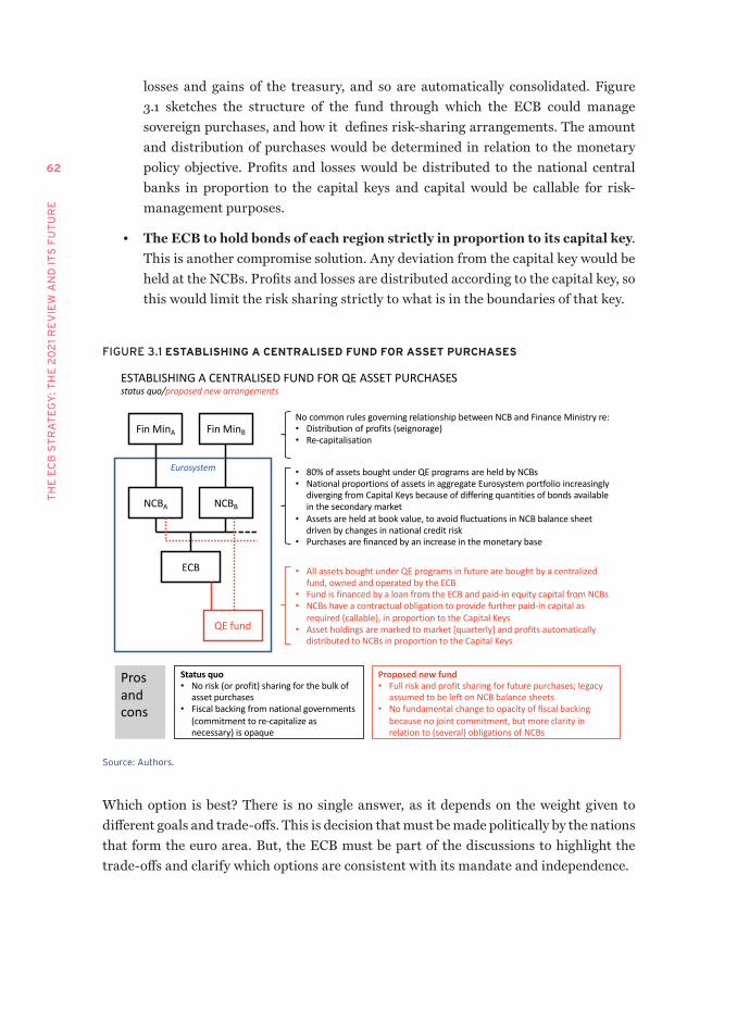
TH
E E
CB
ST
RA
TE
GY
: TH
E 2
02
1 R
EV
IEW
AN
D I
TS
FU
TU
RE
62
losses and gains of the treasury, and so are automatically consolidated. Figure 3.1 sketches the structure of the fund through which the ECB could manage sovereign purchases, and how it defines risk-sharing arrangements. The amount and distribution of purchases would be determined in relation to the monetary policy objective. Profits and losses would be distributed to the national central banks in proportion to the capital keys and capital would be callable for risk-management purposes.
• The ECB to hold bonds of each region strictly in proportion to its capital key. This is another compromise solution. Any deviation from the capital key would be held at the NCBs. Profits and losses are distributed according to the capital key, so this would limit the risk sharing strictly to what is in the boundaries of that key.
FIGURE 3.1 ESTABLISHING A CENTRALISED FUND FOR ASSET PURCHASES
Source: Authors.
Which option is best? There is no single answer, as it depends on the weight given to different goals and trade-offs. This is decision that must be made politically by the nations that form the euro area. But, the ECB must be part of the discussions to highlight the trade-offs and clarify which options are consistent with its mandate and independence.
63
FIS
CA
L A
ND
MO
NE
TAR
y IN
TE
RA
CT
ION
S
3.8 INSTITUTIONAL REFORMS
We have argued that monetary and fiscal policy have meaningful interactions, even if fiscal dominance has been ruled out and the central bank is fully independent and focused on price stability. With a large central bank’s balance sheet and a high level of government debt, these interactions are more sizeable. This is a difficult problem anywhere, but it is particularly difficult when fiscal decisions are decentralised, but monetary policy is not.
We have also pointed out that there are circumstances in which monetary policy is less effective either because of the zero lower bound or because of the nature of the shocks affecting the economy. In such circumstances, some form of fiscal-monetary coordination could be an effective way to achieve price stability.6 In particular in the euro area, the combination of fiscal rules at the national level and centralised monetary policy may lead to a combination of fiscal and monetary policy which is either ineffective in achieving price stability or an excessive burden for the central bank, with undesirable side effects.7 This point has been made by the ECB in several occasions, for example by Draghi (2014), Lagarde (2020), and Schnabel (2021), and reiterated in the recent strategy review.
In unitary systems such as in the US and the UK, informal coordination is achieved by regular meetings between the ministry of finance and the central bank. Although regular informal meetings between fiscal authorities and the ECB president are also envisaged in the euro area, these meetings are not informed by a common analysis of joint monetary and fiscal issues from a union-wide perspective.
A new board for euro area joint fiscal-monetary oversight is one solution. It would be chaired by the ECB but include fiscal authorities, with representation based on different criteria. The board should also be informed by an independent scientific committee issuing a regular report on the fiscal-monetary stance and charged with identifying potential fiscal-monetary crosswinds. The goal would be analysis and oversight, and it would provide a forum for discussion. It could issue warnings and occasional non-binding recommendations with the aim of supporting independent decisions by the ECB and the fiscal authorities.
The complicated governance of the euro area may seem excessively burdened by committees already, but one must not forget that committees have played a key role in the history of the euro area’s formation and in building common culture as a prerequisite for building the EU’s institutions.8 Since the GFC, committees have built new infrastructure, in particular for monitoring risks in the financial sector. An interesting model for a monetary-fiscal board could be the ESRB, responsible for the macroprudential oversight
6 See Bartsch et al. (2020) for a general analysis and Reichlin et al. (2013) for a discussion of fiscal-monetary coordination as an alternative to helicopter money.
7 See Reichlin et al. (2021a) for an empirical evaluation of the fiscal-monetary interactions in conventional and unconventional monetary policy in the euro area.
8 See james (2012) on this point.
TH
E E
CB
ST
RA
TE
GY
: TH
E 2
02
1 R
EV
IEW
AN
D I
TS
FU
TU
RE
64
of the EU financial system and the prevention and mitigation of systemic risk. The ESRB has a broad remit, covering banks, insurers, asset managers, shadow banks, financial market infrastructures and other financial institutions and markets. Its mandate is to assesses systemic risks and, where appropriate, issue warnings and recommendations. The monetary-fiscal board could borrow from that model. It would have to be clear that its recommendations would be in no way binding for monetary policy decisions, the independence of which has to be protected. Giving the chairmanship to the president of the ECB would also be a guarantee that this principle would be respected.
65
CHAPTER 4
Climate change and monetary policy
SUMMARY RECOMMENDATIONS
• The ECB has presented a detailed action plan to include climate change considerations in its monetary policy strategy. We welcome the intention to enhance macroeconomic modelling frameworks with regard to climate change, and further present our own analysis on a number of issues related to the topic.
• We also welcome the ECB’s commitment to a detailed two- to three-year roadmap on climate-related actions for monetary operations.
○ We agree with the ECB that taking climate risk into account in monetary operation is mostly a question of good design, not principle. It requires further work on disclosure, risk assessment, and standards.
○ Monetary operations always need to be designed to optimise across operational objectives such as maximising the effectiveness of monetary policy, minimising valuation risks, and preserving operational flexibility. We stress that there will be a series of trade-offs across different goals of operations to consider.
○ Greening of monetary operations could be achieved by adjusting benchmarks, pricing, haircuts, tilting, negative or positive screening for credit policies, collateral policies, and asset purchases.
• Central banks need to take climate-related financial risks into account to protect their assets. Sound financial risk management suggests that central banks apply environmental, social and governance (ESG) risk metrics and climate stress testing to their own portfolios in accordance with the EU directive. Central banks may use positive screening and tilting in their asset purchases to avoid reproducing ‘brown’ biases in a market-neutral portfolio.
• The ECB should, as discussed in Chapter 1, develop a coherent policy framework to consider secondary objectives such as climate change mitigation and to evaluate the costs of instruments to achieve primary and secondary objectives.
• Higher carbon taxes do not have to be inflationary. The case of British Columbia suggests that a carbon tax changed relative prices and reduced emissions but did not increase the overall price level. The (slightly deflationary) effect was mainly on relative prices rather than on the general price level.
TH
E E
CB
ST
RA
TE
GY
: TH
E 2
02
1 R
EV
IEW
AN
D I
TS
FU
TU
RE
66
• We present empirical evidence on the impact of carbon taxes on inflation. We use a large-scale macroeconomic model (G-Cubed) to quantify the effects under different monetary policy rules.
○ The response of monetary policy to climate policy is important for macroeconomic outcomes. Depending on the monetary policy reaction, the initial shock would amplify output costs and induce deflation or minimise output costs but allow higher inflation in the short run. This is shown through simulations of three monetary policy rules in a global, multisector model (G-Cubed) following a carbon tax of €50 per tonne with a 3% increase per annum. The overall inflation effect is muted in these simulations. As in all models, the caveat is that this is subject to uncertainty and assumptions, for example, the type of redistribution of the carbon tax.
○ Monetary policy rules matter for inflation targets. In our simulations, a forward-looking rule leads to deflation and a sharp drop in GDP due to excessively tight monetary policy. Rules that give weight to present and future inflation, resembling the proposed averaging rule in Chapter 1, have better outcomes. This suggests climate policies and monetary policies may have meaningful interactions, reinforcing the case of considering climate change in the monetary policy framework as a secondary goal
INTRODUCTION
Central banks have not, historically, had climate-related objectives. The primary mandate of the ECB is to pursue price stability and to support – without prejudice to the pursuit of price stability – the general economic policies in the EU. Chapter 1 also discussed how the ECB might incorporate secondary objectives in its policy considerations. There are already several possible candidate secondary policies, including financial frictions, financial stability threats – and climate change.
Climate change may well be the source of the next global crisis, and climate risks represent substantial financial risks that need to be managed in supervisory policy, monetary operations, and the interaction between climate, macroeconomy and monetary policy. We will not attempt to summarise the intense supervisory and regulatory activity.
67
CL
IMA
TE
CH
AN
GE
AN
D M
ON
ETA
Ry
PO
LIC
y
Regarding greening monetary operations, in December 2020 Bloomberg reported that a survey of the Network for Greening the Financial System found that:
“[A] large majority of respondents have taken initial steps in adopting some form of sustainable and responsible investment practices in some of their portfolios, or are planning to do so, with green bond investing, negative screening and ESG integration appear to be becoming popular investment strategies.” 9
We will briefly review the state of this debate below.
The macroeconomic impact of climate risks and climate policies has received less attention than financial stability. This may, in part, be due to the difficulties in jointly modelling highly uncertain long-run processes like the physical impact of global warming and future technology and innovation. Nevertheless, climate shocks and climate policies may impact monetary policy significantly through their effect on output and inflation. In particular:
• Climate change may impact output volatility if the frequency of natural disasters worldwide increases, resulting in recurring negative supply disruptions.
• Climate policies – CO2 pricing and regulation of CO2 in particular – can impact output growth rates in the transition from a high to a low emission economy (see Box 4.1 for an overview of the research that quantifies abatements costs).
• Rising CO2 (shadow) prices will invariably change relative prices but may also exert upward inflation pressure.
Plausibly, the combined effect of higher physical risk and increasing CO2 taxes might lead to stagnation. One key question is how climate mitigation (carbon taxes or carbon prices) would impact inflation. Would a secular increase in the price of carbon (and carbon equivalents) not only affect relative prices, but also put upward pressure on the price level? How significant is this effect likely to be? How much does this effect depend on the reaction function of monetary policy?
The main focus of this chapter is to provide new evidence on the link between climate policies and monetary policies, in particular how carbon taxes impact inflation under different monetary policy reactions. By making this link clear and assessing its strength, central banks will be better placed to consider how their monetary policy strategy can incorporate the effects of climate policies.
We explore the case of British Columbia since it is often seen as the exemplar of carbon taxation. Our findings suggest that carbon taxes had no inflationary impact; if anything, we find a deflationary impact. We use a large-scale multi-country multisector model (G-Cubed) to estimate the magnitude of these effects in different monetary regimes.
9 Source: www.bloomberg.com/news/articles/2020-12-15/central-banks-preach-green-with-decisive-actions-yet-to-follow
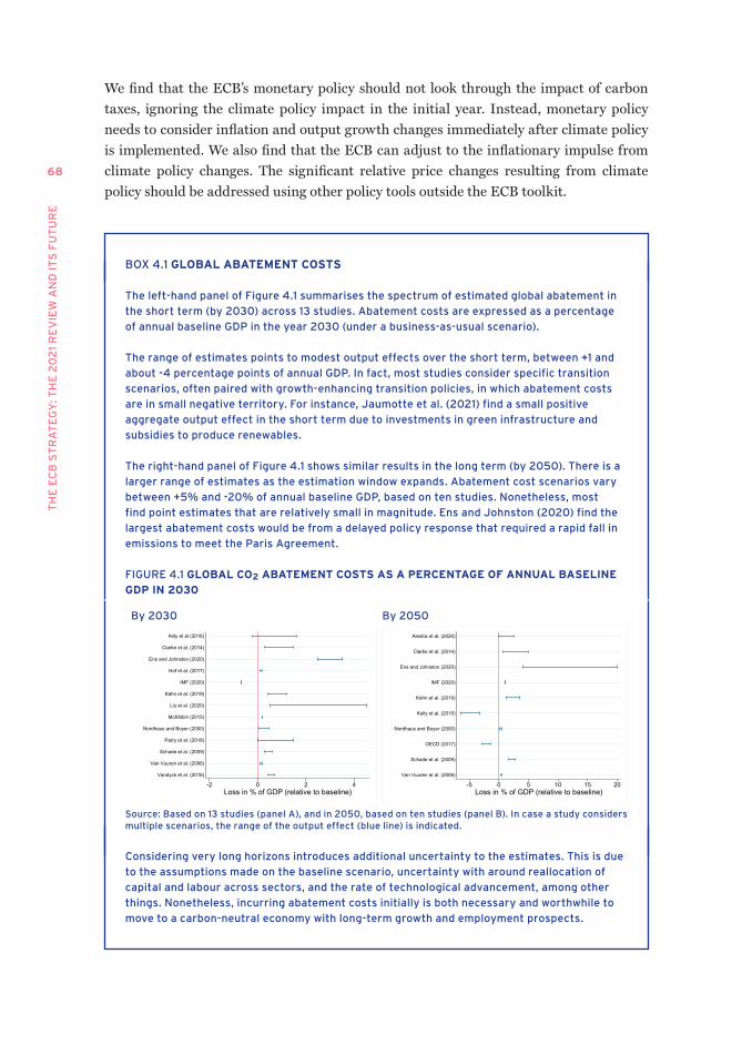
TH
E E
CB
ST
RA
TE
GY
: TH
E 2
02
1 R
EV
IEW
AN
D I
TS
FU
TU
RE
68
We find that the ECB’s monetary policy should not look through the impact of carbon taxes, ignoring the climate policy impact in the initial year. Instead, monetary policy needs to consider inflation and output growth changes immediately after climate policy is implemented. We also find that the ECB can adjust to the inflationary impulse from climate policy changes. The significant relative price changes resulting from climate policy should be addressed using other policy tools outside the ECB toolkit.
BOX 4.1 GLOBAL ABATEMENT COSTS
The left-hand panel of Figure 4.1 summarises the spectrum of estimated global abatement in
the short term (by 2030) across 13 studies. Abatement costs are expressed as a percentage
of annual baseline GDP in the year 2030 (under a business-as-usual scenario).
The range of estimates points to modest output effects over the short term, between +1 and
about -4 percentage points of annual GDP. In fact, most studies consider specific transition
scenarios, often paired with growth-enhancing transition policies, in which abatement costs
are in small negative territory. For instance, Jaumotte et al. (2021) find a small positive
aggregate output effect in the short term due to investments in green infrastructure and
subsidies to produce renewables.
The right-hand panel of Figure 4.1 shows similar results in the long term (by 2050). There is a
larger range of estimates as the estimation window expands. Abatement cost scenarios vary
between +5% and -20% of annual baseline GDP, based on ten studies. Nonetheless, most
find point estimates that are relatively small in magnitude. Ens and Johnston (2020) find the
largest abatement costs would be from a delayed policy response that required a rapid fall in
emissions to meet the Paris Agreement.
FIGURE 4.1 GLOBAL CO2 ABATEMENT COSTS AS A PERCENTAGE OF ANNUAL BASELINE
GDP IN 2030
By 2030
Vandyck et al. (2016)
Van Vuuren et al. (2006)
Schade et al. (2009)
Parry et al. (2018)
Nordhaus and Boyer (2000)
McKibbin (2015)
Liu et al. (2020)
Kahn et al. (2019)
IMF (2020)
Hof et al. (2017)
Ens and Johnston (2020)
Clarke et al. (2014)
Aldy et al (2016)
-2 0 2 4Loss in % of GDP (relative to baseline)
By 2050
Van Vuuren et al. (2006)
Schade et al. (2009)
OECD (2017)
Nordhaus and Boyer (2000)
Kelly et al. (2015)
Kahn et al. (2019)
IMF (2020)
Ens and Johnston (2020)
Clarke et al. (2014)
Alestra et al. (2020)
-5 0 5 10 15 20Loss in % of GDP (relative to baseline)
Source: Based on 13 studies (panel A), and in 2050, based on ten studies (panel B). In case a study considers multiple scenarios, the range of the output effect (blue line) is indicated.
Considering very long horizons introduces additional uncertainty to the estimates. This is due
to the assumptions made on the baseline scenario, uncertainty with around reallocation of
capital and labour across sectors, and the rate of technological advancement, among other
things. Nonetheless, incurring abatement costs initially is both necessary and worthwhile to
move to a carbon-neutral economy with long-term growth and employment prospects.
69
CL
IMA
TE
CH
AN
GE
AN
D M
ON
ETA
Ry
PO
LIC
y
4.1 HOW SHOULD CENTRAL BANK OPERATIONS INCORPORATE CLIMATE
RISK?
Should climate risk play any role in central bank monetary policy operations? Previously the consensus was a firm ‘no’. Today, the response is more nuanced. In the February 2021 CfM Survey of Macroeconomists, more than 80% of respondents favoured a change in ECB policy to address the environmental impact of bond-purchasing policies. However, only 40% supported a change in the legal mandate to include carbon neutrality (CfM 2021).
Climate-related financial risks will invariably affect central bank operations and their financial assets, such that, at least, a ‘protective’ approach will be needed. Central bank balance sheets are large, and the assets they hold could be exposed to climate-related shocks in the same manner as any large asset manager’s portfolio. Prudence and sound financial risk management strongly suggest that central banks apply similar criteria and stress tests to those they deploy in their supervision of financial institutions. Protecting central bank assets from financial risk will mean using risk metrics and policies that take climate risk into account.
Supervisors are taking seriously the possibility that climate risk could translate directly into financial stability risk, and are deploying new policy tools such as climate stress-testing to assess the extent to which financial intermediaries may be exposed to these risks; also as a tool to ‘internalise’ them in risk management systems. These standards should be applied to central bank portfolios as well.
The IFRS Foundation is leading a consolidation effort to provide a global baseline on climate reporting standards for companies to adopt. This work is supported by the ISOCO and the FSB and has been welcomed by the G7 and the G20. At the same time, the EU has started to measure climate-related risks that focus not only on disclosure of the impact of climate change (and its mitigation policies) on the value of companies, but also on disclosure to assess the impact that companies have on our climate.
This higher level of ambition is linked to the specific objectives of the EU Green Deal and is supported by a specific legislative effort. The ECB, as an EU institution, should aim at complying with EU standards. At the same time, as a major global participant in the global capital market, it should assist the effort to achieve interoperability between the global reporting baseline and EU-specific requirements.
Central banks also play a crucial role as buyers of assets and, in some instances, as market makers, which could support a more proactive approach to climate risks. The ECB could tilt its corporate bond purchases towards green assets in line with a secondary objective (Chapter 1). The ECB could use its market-making power to promote new green asset
TH
E E
CB
ST
RA
TE
GY
: TH
E 2
02
1 R
EV
IEW
AN
D I
TS
FU
TU
RE
70
classes, in a departure from the traditional benchmark of market neutrality.10 At first sight, market neutrality may seem like a reasonable guideline, but as Schnabel (2020, 2021) has pointed out, it suffers from a flaw: market neutrality will depart from market efficiency if externalities are present. Markets fail to allocate resources efficiently when polluting firms gain an advantage over clean firms if polluting firms do not pay the total cost of their production. As a result, the market will be composed of many polluting firms and few clean ones. The assets held by the ECB exhibit a brown ‘emissions bias’, as shown by Papoutsi et al. (2021). The task of internalising externalities by imposing regulation or CO2 taxes falls on governments, not central banks. But when internalisation is not perfect, central banks that uphold market neutrality distort asset prices and are conducting de facto ‘brown QE’.
A more differentiated discussion of the pros and cons of ‘green QE’ would recognise that it is not a binary ‘yes or no’ choice. Instead, monetary operations involve many instruments and several goals:
• Monetary operations comprise credit operations, collateral policies as well as asset purchases. Policies for each have several margins which may reflect and affect climate risks. Collateral policies, for instance, involve choices about the size of haircuts for different (climate) risk classes. The same is true for credit policies: sound risk management means that credit policies must account for climate risk when deciding on eligibility, pricing, and collateral requirements of different counterparts.
• Monetary operations are guided by more than one goal. Operations are designed to maximise the effectiveness of the monetary policy. At the same time, they should minimise the risk to the central bank’s balance sheet, provide operational flexibility, and be designed to contribute to mitigation of climate change.
4.1.1 The existence of multiple goals and instruments implies that there are
trade-offs
A comparative assessment of these trade-offs for generic operations has recently been provided by the NGFS (2021). Table 4.1, taken from the NGFS report, shows that potential changes to existing policies and instruments can spill over positively and negatively to different objectives.
10 Market neutrality means buying assets in the same proportions as their existing market share. If brown bonds, for instance, issued by companies in the coal sector, made up most of the market capitalisation then the central bank would have to purchase mostly brown assets. The idea behind market neutrality is that central banks should not introduce any bias in relative asset prices through monetary operations.
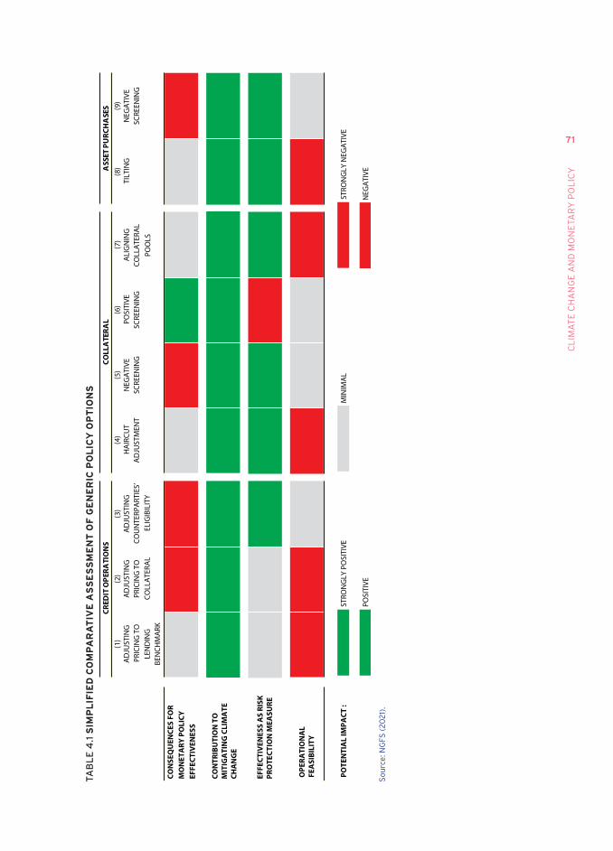
71
CL
IMA
TE
CH
AN
GE
AN
D M
ON
ETA
Ry
PO
LIC
y
TAB
LE
4.1
SIM
PL
IFIE
D C
OM
PA
RA
TIv
E A
SS
ES
SM
EN
T O
F G
EN
ER
IC P
OL
ICY
OP
TIO
NS
AD
JUST
ING
PR
ICIN
G T
O
LEN
DIN
G
BEN
CH
MA
RK
AD
JUST
ING
PR
ICIN
G T
O
CO
LLA
TERA
L
AD
JUST
ING
C
OU
NTE
RPA
RTIE
S’
ELIG
IBIL
ITY
HA
IRC
UT
AD
JUST
MEN
TN
EGA
TIVE
SC
REEN
ING
POSI
TIVE
SC
REEN
ING
ALI
GN
ING
C
OLL
ATE
RAL
POO
LS
TILT
ING
NEG
ATI
VE
SCRE
ENIN
G
CON
SEQ
UEN
CES
FOR
MO
NET
ARY
PO
LICY
EF
FECT
IVEN
ESS
CRE
DIT
OPE
RATI
ON
SCO
LLA
TERA
LA
SSET
PU
RCH
ASE
S
CON
TRIB
UTI
ON
TO
MIT
IGA
TIN
G C
LIM
ATE
CHA
NG
E
EFFE
CTIV
ENES
S A
S RI
SK
PRO
TECT
ION
MEA
SURE
OPE
RATI
ON
AL
FEA
SIBI
LITY
POTE
NTI
AL
IMPA
CT :
STRO
NG
LY P
OSI
TIVE
MIN
IMA
LST
RON
GLY
NEG
ATI
VE
POSI
TIVE
NEG
ATI
VE
(1)
(2)
(3)
(4)
(5)
(6)
(7)
(8)
(9)
So
urc
e: N
GFS
(2
02
1).
TH
E E
CB
ST
RA
TE
GY
: TH
E 2
02
1 R
EV
IEW
AN
D I
TS
FU
TU
RE
72
In Table 4.1, green fields show that the option is favourable for achieving a goal, whereas red fields show detrimental impacts. For instance:
• Column 3: Exclusion of counterparties from credit operations based on their climate assessments. This would severely limit the effectiveness of monetary policy (dark red) while being only mildly positive on mitigation of climate change or climate risks (light green).
• Column 6: Positive screening for ‘green’ assets. This is highly effective (dark green) in contributing to mitigating climate change, mildly positive for the effectiveness of monetary policy (light green). mildly detrimental from a pure risk perspective (light red), and neutral for operational flexibility.
• Column 9: Negative screening of asset purchases, excluding ‘brown’ assets from purchases. This has a mildly positive effect on the climate and risk reduction, but a mildly negative effect on monetary policy effectiveness. because it reduces the universe of investable assets.
More research will further refine and quantify this trade-off matrix. It could also be expanded to other areas of concern for policymakers; for example, climate change links may make monetary policy seem more relatable to the general public, making communication easier, but they may also complicate the messaging of monetary policy communication. Even this first assessment clearly illustrates that there is no perfect instrument that involves no trade-offs. It also shows that design matters when greening monetary operations, and that the discussion about how to implement climate risk in monetary operations has moved from a black-and-white one to more nuanced shades of green and red. Therefore, the assessment should now become technical rather than principled.
4.2 CARBON TAxING AND PRICE DYNAMICS: EvIDENCE FROM BRITISH
COLUMBIA11
As mentioned above, the existing research yields very little that would allow us to estimate the effect of carbon taxes on prices and inflation. The effects would depend on design features such as the magnitude, the initial level, expected growth rate, and the volatility and redistribution of any pricing and taxing scheme.
British Columbia (BC), a province of Canada, provides an excellent model to study carbon taxes: since 2008, it has implemented a well-designed tax of significant magnitude. In 2008 the tax was set at CA$10, and scheduled to increase every year until 2012, at which point it remained at CA$30 per tonne of CO2. Following expert advice, the price
11 This section was co-authored with Maximilian Konradt.
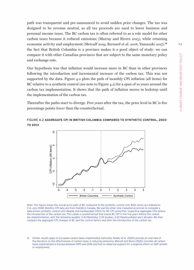
73
CL
IMA
TE
CH
AN
GE
AN
D M
ON
ETA
Ry
PO
LIC
y
path was transparent and pre-announced to avoid sudden price changes. The tax was designed to be revenue neutral, as all tax proceeds are used to lower business and personal income taxes. The BC carbon tax is often referred to as a role model for other carbon taxes because it reduced emissions (Murray and Rivers 2015), while retaining economic activity and employment (Metcalf 2019, Bernard et al. 2018, Yamazaki 2017).12 the fact that British Columbia is a province makes it a good object of study: we can compare it with other Canadian provinces that are subject to the same monetary policy and exchange rate.
Our hypothesis was that inflation would increase more in BC than in other provinces following the introduction and incremental increase of the carbon tax. This was not supported by the data. Figure 4.2 plots the path of monthly CPI inflation (all items) for BC relative to a synthetic control (see note to Figure 4.2) for a span of 10 years around the carbon tax implementation. It shows that the path of inflation moves in lockstep until the implementation of the carbon tax.
Thereafter the paths start to diverge. Five years after the tax, the price level in BC is five percentage points lower than the counterfactual.
FIGURE 4.2 AGGREGATE CPI IN BRITISH COLUMBIA COMPARED TO SYNTHETIC CONTROL, 2003
TO 2013
-10
-50
510
CPI
infla
tion
(All
item
s)
-5 -4 -3 -2 -1 0 1 2 3 4 5
British Columbia Synthetic Control
Note: This figure shows the overall price path of BC compared to the synthetic control unit. Both series are indexed to 0 in july 2008. Monthly CPI data are from Statistics Canada. We use the other nine Canadian provinces to compute a data-driven synthetic control unit (Abadie and Gardeazabel 2003) for BC CPI using their respective aggregate CPIs before the introduction of the carbon tax. This yields a counterfactual that tracks BC CPI in the five years before the carbon tax implementation, with the following weights: 0.43 Manitoba, 0.35 Quebec, 0.22 Newfoundland and Labrador. We then compare the aggregate CPI changes of BC and the control before and after the introduction of the carbon tax.
12 Similar results apply to European carbon taxes implemented nationally. Rafaty et al. (2020) provide an overview of the literature on the effectiveness of carbon taxes in reducing emissions. Metcalf and Stock (2020) consider all carbon taxes implemented in Europe between 1990 and 2018 and find no empirical support for a negative effect on GDP growth or employment.
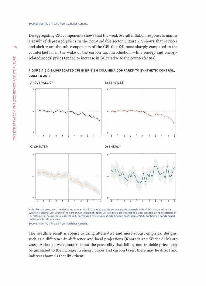
TH
E E
CB
ST
RA
TE
GY
: TH
E 2
02
1 R
EV
IEW
AN
D I
TS
FU
TU
RE
74
Source: Monthly CPI data from Statistics Canada.
Disaggregating CPI components shows that the weak overall inflation response is mainly a result of depressed prices in the non-tradable sector. Figure 4.3 shows that services and shelter are the sub-components of the CPI that fell most sharply compared to the counterfactual in the wake of the carbon tax introduction, while energy and energy-related goods’ prices tended to increase in BC relative to the counterfactual.
FIGURE 4.3 DISAGGREGATED CPI IN BRITISH COLUMBIA COMPARED TO SYNTHETIC CONTROL,
2003 TO 2013
A) OVERALL CPI
-10
010
-5 -4 -3 -2 -1 0 1 2 3 4 5
B) SERVICES
-10
010
-5 -4 -3 -2 -1 0 1 2 3 4 5
C) SHELTER
-10
010
-5 -4 -3 -2 -1 0 1 2 3 4 5
D) ENERGY
-10
010
-5 -4 -3 -2 -1 0 1 2 3 4 5
Note: This figure shows the deviation of overall CPI (panel a) and its sub-categories (panels b-d) of BC compared to the synthetic control unit around the carbon tax implementation. All variables are expressed as percentage point deviations of BC relative to the synthetic control unit, normalised to 0 in july 2008. Shaded areas depict 95% confidence bands based on the pre-tax differences.
Source: Monthly CPI data from Statistics Canada.
The headline result is robust to using alternative and more robust empirical designs, such as a difference-in-difference and local projections (Konradt and Weder di Mauro 2021). Although we cannot rule out the possibility that falling non-tradable prices may be unrelated to the increase in energy prices and carbon taxes, there may be direct and indirect channels that link them:
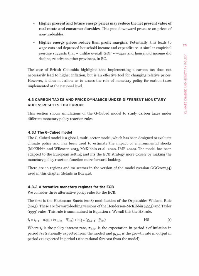
75
CL
IMA
TE
CH
AN
GE
AN
D M
ON
ETA
Ry
PO
LIC
y
• Higher present and future energy prices may reduce the net present value of real estate and consumer durables. This puts downward pressure on prices of non-tradeables.
• Higher energy prices reduce firm profit margins. Potentially, this leads to wage cuts and depressed household income and expenditure. A similar empirical exercise suggests that – unlike overall GDP – wages and household income did decline, relative to other provinces, in BC.
The case of British Columbia highlights that implementing a carbon tax does not necessarily lead to higher inflation, but is an effective tool for changing relative prices. However, it does not allow us to assess the role of monetary policy for carbon taxes implemented at the national level.
4.3 CARBON TAxES AND PRICE DYNAMICS UNDER DIFFERENT MONETARY
RULES: RESULTS FOR EUROPE
This section shows simulations of the G-Cubed model to study carbon taxes under different monetary policy reaction rules.
4.3.1 The G-Cubed model
The G-Cubed model is a global, multi-sector model, which has been designed to evaluate climate policy and has been used to estimate the impact of environmental shocks (McKibbin and Wilcoxen 2013, McKibbin et al. 2020, IMF 2020). The model has been adapted to the European setting and fits the ECB strategy more closely by making the monetary policy reaction function more forward-looking.
There are 10 regions and 20 sectors in the version of the model (version GGG20v154) used in this chapter (details in Box 4.2).
4.3.2 Alternative monetary regimes for the ECB
We consider three alternative policy rules for the ECB.
The first is the Hartmann-Smets (2018) modification of the Orphanides-Wieland Rule (2013). These are forward-looking versions of the Henderson-McKibbin (1993) and Taylor (1993) rules. This rule is summarised in Equation 1. We call this the HS rule.
it = it–1 + 0.34 * (πt,t+1 – πt+1) + 0.4 * (gt,t+1 – gt+1) HS (1)
Where it is the policy interest rate, πt,t+1 is the expectation in period t of inflation in period t+1 (rationally expected from the model) and gt,t+1 is the growth rate in output in period t+1 expected in period t (the rational forecast from the model)
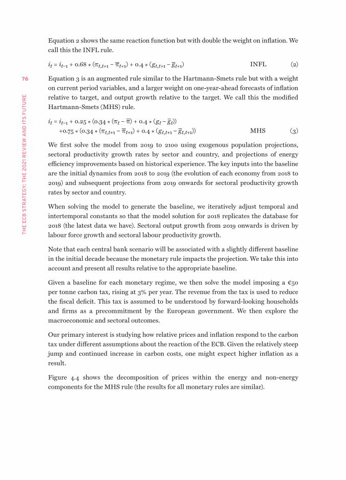
TH
E E
CB
ST
RA
TE
GY
: TH
E 2
02
1 R
EV
IEW
AN
D I
TS
FU
TU
RE
76
Equation 2 shows the same reaction function but with double the weight on inflation. We call this the INFL rule.
it = it–1 + 0.68 * (πt,t+1 – πt+1) + 0.4 * (gt,t+1 – gt+1) INFL (2)
Equation 3 is an augmented rule similar to the Hartmann-Smets rule but with a weight on current period variables, and a larger weight on one-year-ahead forecasts of inflation relative to target, and output growth relative to the target. We call this the modified Hartmann-Smets (MHS) rule.
it = it–1 + 0.25 * (0.34 * (πt – π) + 0.4 * (gt – gt)) +0.75 * (0.34 * (πt,t+1 – πt+1) + 0.4 * (gt,t+1 – gt,t+1)) MHS (3)
We first solve the model from 2019 to 2100 using exogenous population projections, sectoral productivity growth rates by sector and country, and projections of energy efficiency improvements based on historical experience. The key inputs into the baseline are the initial dynamics from 2018 to 2019 (the evolution of each economy from 2018 to 2019) and subsequent projections from 2019 onwards for sectoral productivity growth rates by sector and country.
When solving the model to generate the baseline, we iteratively adjust temporal and intertemporal constants so that the model solution for 2018 replicates the database for 2018 (the latest data we have). Sectoral output growth from 2019 onwards is driven by labour force growth and sectoral labour productivity growth.
Note that each central bank scenario will be associated with a slightly different baseline in the initial decade because the monetary rule impacts the projection. We take this into account and present all results relative to the appropriate baseline.
Given a baseline for each monetary regime, we then solve the model imposing a €50 per tonne carbon tax, rising at 3% per year. The revenue from the tax is used to reduce the fiscal deficit. This tax is assumed to be understood by forward-looking households and firms as a precommitment by the European government. We then explore the macroeconomic and sectoral outcomes.
Our primary interest is studying how relative prices and inflation respond to the carbon tax under different assumptions about the reaction of the ECB. Given the relatively steep jump and continued increase in carbon costs, one might expect higher inflation as a result.
Figure 4.4 shows the decomposition of prices within the energy and non-energy components for the MHS rule (the results for all monetary rules are similar).
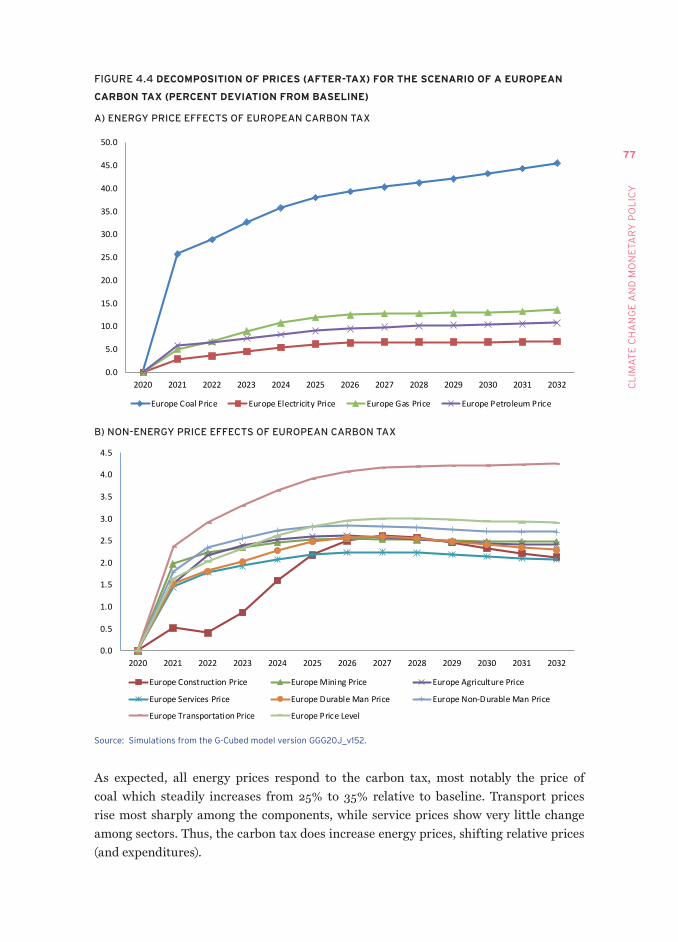
77
CL
IMA
TE
CH
AN
GE
AN
D M
ON
ETA
Ry
PO
LIC
y
FIGURE 4.4 DECOMPOSITION OF PRICES (AFTER-TAx) FOR THE SCENARIO OF A EUROPEAN
CARBON TAx (PERCENT DEvIATION FROM BASELINE)
A) ENERGY PRICE EFFECTS OF EUROPEAN CARBON TAX
0.0
5.0
10.0
15.0
20.0
25.0
30.0
35.0
40.0
45.0
50.0
2020 2021 2022 2023 2024 2025 2026 2027 2028 2029 2030 2031 2032
Europe Coal Price Europe Electricity Price Europe Gas Price Europe Petroleum Price
B) NON-ENERGY PRICE EFFECTS OF EUROPEAN CARBON TAX
0.0
0.5
1.0
1.5
2.0
2.5
3.0
3.5
4.0
4.5
2020 2021 2022 2023 2024 2025 2026 2027 2028 2029 2030 2031 2032
Europe Construction Price Europe Mining Price Europe Agriculture Price
Europe Services Price Europe Durable Man Price Europe Non-Durable Man Price
Europe Transportation Price Europe Price Level
Source: Simulations from the G-Cubed model version GGG20j_v152.
As expected, all energy prices respond to the carbon tax, most notably the price of coal which steadily increases from 25% to 35% relative to baseline. Transport prices rise most sharply among the components, while service prices show very little change among sectors. Thus, the carbon tax does increase energy prices, shifting relative prices (and expenditures).
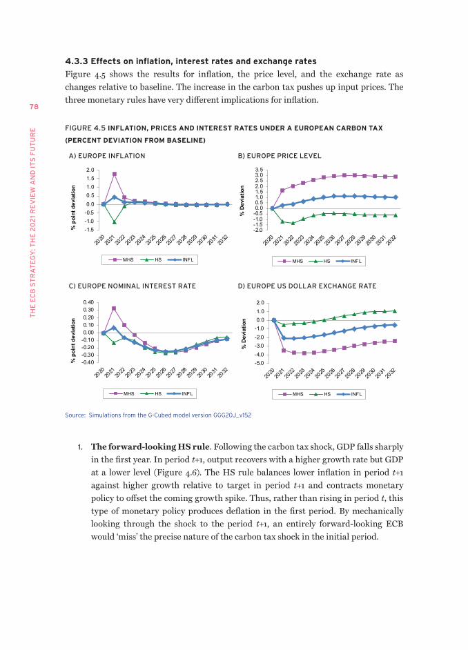
TH
E E
CB
ST
RA
TE
GY
: TH
E 2
02
1 R
EV
IEW
AN
D I
TS
FU
TU
RE
78
4.3.3 Effects on inflation, interest rates and exchange rates
Figure 4.5 shows the results for inflation, the price level, and the exchange rate as changes relative to baseline. The increase in the carbon tax pushes up input prices. The three monetary rules have very different implications for inflation.
FIGURE 4.5 INFLATION, PRICES AND INTEREST RATES UNDER A EUROPEAN CARBON TAx
(PERCENT DEvIATION FROM BASELINE)
A) EUROPE INFLATION
-1.5-1.0-0.50.00.51.01.52.0
2020202120222023202420252026202720282029203020312032
% p
oint
dev
iatio
n
MHS HS INFL
B) EUROPE PRICE LEVEL
-2.0-1.5-1.0-0.50.00.51.01.52.02.53.03.5
2020202120222023202420252026202720282029203020312032
% D
evia
tion
MHS HS INFL
C) EUROPE NOMINAL INTEREST RATE
-0.40-0.30-0.20-0.100.000.100.200.300.40
2020202120222023202420252026202720282029203020312032
% p
oint
dev
iatio
n
MHS HS INFL
D) EUROPE US DOLLAR EXCHANGE RATE
-5.0-4.0-3.0-2.0-1.00.01.02.0
2020202120222023202420252026202720282029203020312032
% D
evia
tion
MHS HS INFL
Source: Simulations from the G-Cubed model version GGG20j_v152
1. The forward-looking HS rule. Following the carbon tax shock, GDP falls sharply in the first year. In period t+1, output recovers with a higher growth rate but GDP at a lower level (Figure 4.6). The HS rule balances lower inflation in period t+1 against higher growth relative to target in period t+1 and contracts monetary policy to offset the coming growth spike. Thus, rather than rising in period t, this type of monetary policy produces deflation in the first period. By mechanically looking through the shock to the period t+1, an entirely forward-looking ECB would ‘miss’ the precise nature of the carbon tax shock in the initial period.
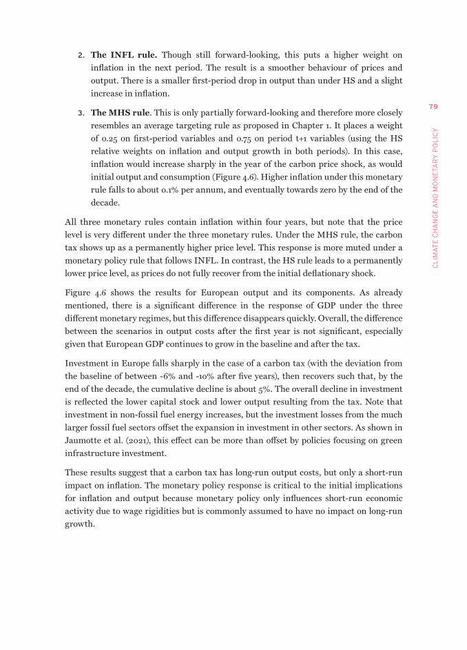
79
CL
IMA
TE
CH
AN
GE
AN
D M
ON
ETA
Ry
PO
LIC
y
2. The INFL rule. Though still forward-looking, this puts a higher weight on inflation in the next period. The result is a smoother behaviour of prices and output. There is a smaller first-period drop in output than under HS and a slight increase in inflation.
3. The MHS rule. This is only partially forward-looking and therefore more closely resembles an average targeting rule as proposed in Chapter 1. It places a weight of 0.25 on first-period variables and 0.75 on period t+1 variables (using the HS relative weights on inflation and output growth in both periods). In this case, inflation would increase sharply in the year of the carbon price shock, as would initial output and consumption (Figure 4.6). Higher inflation under this monetary rule falls to about 0.1% per annum, and eventually towards zero by the end of the decade.
All three monetary rules contain inflation within four years, but note that the price level is very different under the three monetary rules. Under the MHS rule, the carbon tax shows up as a permanently higher price level. This response is more muted under a monetary policy rule that follows INFL. In contrast, the HS rule leads to a permanently lower price level, as prices do not fully recover from the initial deflationary shock.
Figure 4.6 shows the results for European output and its components. As already mentioned, there is a significant difference in the response of GDP under the three different monetary regimes, but this difference disappears quickly. Overall, the difference between the scenarios in output costs after the first year is not significant, especially given that European GDP continues to grow in the baseline and after the tax.
Investment in Europe falls sharply in the case of a carbon tax (with the deviation from the baseline of between -6% and -10% after five years), then recovers such that, by the end of the decade, the cumulative decline is about 5%. The overall decline in investment is reflected the lower capital stock and lower output resulting from the tax. Note that investment in non-fossil fuel energy increases, but the investment losses from the much larger fossil fuel sectors offset the expansion in investment in other sectors. As shown in Jaumotte et al. (2021), this effect can be more than offset by policies focusing on green infrastructure investment.
These results suggest that a carbon tax has long-run output costs, but only a short-run impact on inflation. The monetary policy response is critical to the initial implications for inflation and output because monetary policy only influences short-run economic activity due to wage rigidities but is commonly assumed to have no impact on long-run growth.
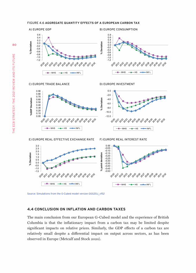
TH
E E
CB
ST
RA
TE
GY
: TH
E 2
02
1 R
EV
IEW
AN
D I
TS
FU
TU
RE
80
FIGURE 4.6 AGGREGATE QUANTITY EFFECTS OF A EUROPEAN CARBON TAx
A) EUROPE GDP
-1.2-1.0-0.8-0.6-0.4-0.20.00.20.40.6
2020202120222023202420252026202720282029203020312032
% D
evia
tion
MHS HS INFL
B) EUROPE CONSUMPTION
-1.2-1.0-0.8-0.6-0.4-0.20.00.20.40.60.8
2020202120222023202420252026202720282029203020312032
% D
evia
tion
MHS HS INFL
C) EUROPE TRADE BALANCE
0.000.100.200.300.400.500.600.700.800.90
2020202120222023202420252026202720282029203020312032
%G
DP
Dev
iatio
n
MHS HS INFL
D) EUROPE INVESTMENT
-12.0
-10.0
-8.0
-6.0
-4.0
-2.0
0.0
2020202120222023202420252026202720282029203020312032
% D
evia
tion
MHS HS INFL
E) EUROPE REAL EFFECTIVE EXCHANGE RATE
-1.5-1.0-0.50.00.51.01.52.02.53.0
2020202120222023202420252026202720282029203020312032
% D
evia
tion
MHS HS INFL
F) EUROPE REAL INTEREST RATE
-0.50-0.45-0.40-0.35-0.30-0.25-0.20-0.15-0.10-0.050.00
2020202120222023202420252026202720282029203020312032
% p
oint
dev
iatio
n
MHS HS INFL
Source: Simulations from the G-Cubed model version GGG20j_v152
4.4 CONCLUSION ON INFLATION AND CARBON TAxES
The main conclusion from our European G-Cubed model and the experience of British Columbia is that the inflationary impact from a carbon tax may be limited despite significant impacts on relative prices. Similarly, the GDP effects of a carbon tax are relatively small despite a differential impact on output across sectors, as has been observed in Europe (Metcalf and Stock 2020).
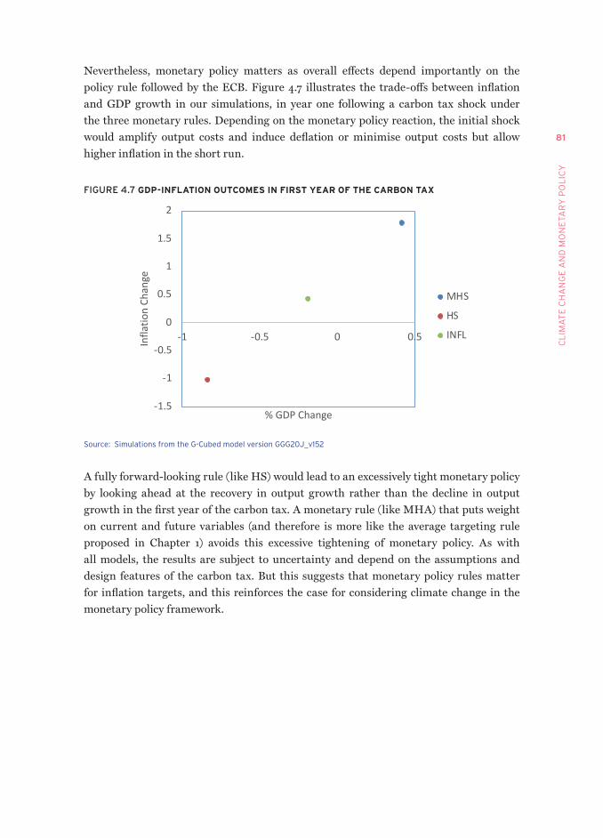
81
CL
IMA
TE
CH
AN
GE
AN
D M
ON
ETA
Ry
PO
LIC
y
Nevertheless, monetary policy matters as overall effects depend importantly on the policy rule followed by the ECB. Figure 4.7 illustrates the trade-offs between inflation and GDP growth in our simulations, in year one following a carbon tax shock under the three monetary rules. Depending on the monetary policy reaction, the initial shock would amplify output costs and induce deflation or minimise output costs but allow higher inflation in the short run.
FIGURE 4.7 GDP-INFLATION OUTCOMES IN FIRST YEAR OF THE CARBON TAx
-1.5
-1
-0.5
0
0.5
1
1.5
2
-1 -0.5 0 0.5Infla
tion
Chan
ge
% GDP Change
MHS
HS
INFL
Source: Simulations from the G-Cubed model version GGG20j_v152
A fully forward-looking rule (like HS) would lead to an excessively tight monetary policy by looking ahead at the recovery in output growth rather than the decline in output growth in the first year of the carbon tax. A monetary rule (like MHA) that puts weight on current and future variables (and therefore is more like the average targeting rule proposed in Chapter 1) avoids this excessive tightening of monetary policy. As with all models, the results are subject to uncertainty and depend on the assumptions and design features of the carbon tax. But this suggests that monetary policy rules matter for inflation targets, and this reinforces the case for considering climate change in the monetary policy framework.

TH
E E
CB
ST
RA
TE
GY
: TH
E 2
02
1 R
EV
IEW
AN
D I
TS
FU
TU
RE
82
BOX 4.2 MAIN FEATURES OF THE G-CUBED MODEL
TABLE 4.2 REGIONS IN THE G-CUBED MODEL
Region Code Region Description
AUS Australia
CHN China
EUW Europe (region, not Euro area)
IND India
JPN Japan
OPC Oil-Exporting developing countries
OEC Rest of the OECD
ROW Rest of the World
RUS Russian Federation
USA United States
The sectors in the model are set out in Table 4.3:
TABLE 4.3 SECTORS IN THE G-CUBED MODEL
Number Sector Name Note
1 Electricity delivery Energy sectors other than generation
2 Gas extraction and utilities
3 Petroleum refining
4 Coal mining
5 Crude oil extraction
6 Construction Goods and services
7 Other mining
8 Agriculture and forestry
9 Durable goods
10 Nondurable goods
11 Transportation
12 Services
13 Coal generation Electricitygeneration sectors
14 Natural gas generation
15 Petroleum generation
16 Nuclear generation
17 Wind generation
18 Solar generation
19 Hydroelectric generation
20 Other generation
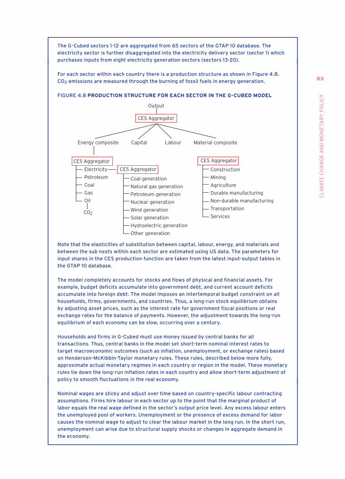
83
CL
IMA
TE
CH
AN
GE
AN
D M
ON
ETA
Ry
PO
LIC
y
The G-Cubed sectors 1-12 are aggregated from 65 sectors of the GTAP 10 database. The
electricity sector is further disaggregated into the electricity delivery sector (sector 1) which
purchases inputs from eight electricity generation sectors (sectors 13-20).
For each sector within each country there is a production structure as shown in Figure 4.8.
CO2 emissions are measured through the burning of fossil fuels in energy generation.
FIGURE 4.8 PRODUCTION STRUCTURE FOR EACH SECTOR IN THE G-CUBED MODEL
Output
CES Aggregator
Energy composite Capital Labour Material composite
CES Aggregator
Electricity
Petroleum
Coal
Gas
Oil
CO2
CES Aggregator
Coal generation
Natural gas generation
Petroleum generation
Nuclear generation
Wind generation
Solar generation
Hydroelectric generation
Other generation
CES Aggregator
Construction
Mining
Agriculture
Durable manufacturing
Non-durable manufacturing
Transportation
Services
Note that the elasticities of substitution between capital, labour, energy, and materials and
between the sub nests within each sector are estimated using US data. The parameters for
input shares in the CES production function are taken from the latest input-output tables in
the GTAP 10 database.
The model completely accounts for stocks and flows of physical and financial assets. For
example, budget deficits accumulate into government debt, and current account deficits
accumulate into foreign debt. The model imposes an intertemporal budget constraint on all
households, firms, governments, and countries. Thus, a long-run stock equilibrium obtains
by adjusting asset prices, such as the interest rate for government fiscal positions or real
exchange rates for the balance of payments. However, the adjustment towards the long-run
equilibrium of each economy can be slow, occurring over a century.
Households and firms in G-Cubed must use money issued by central banks for all
transactions. Thus, central banks in the model set short-term nominal interest rates to
target macroeconomic outcomes (such as inflation, unemployment, or exchange rates) based
on Henderson-McKibbin-Taylor monetary rules. These rules, described below more fully,
approximate actual monetary regimes in each country or region in the model. These monetary
rules tie down the long-run inflation rates in each country and allow short-term adjustment of
policy to smooth fluctuations in the real economy.
Nominal wages are sticky and adjust over time based on country-specific labour contracting
assumptions. Firms hire labour in each sector up to the point that the marginal product of
labor equals the real wage defined in the sector’s output price level. Any excess labour enters
the unemployed pool of workers. Unemployment or the presence of excess demand for labor
causes the nominal wage to adjust to clear the labour market in the long run. In the short run,
unemployment can arise due to structural supply shocks or changes in aggregate demand in
the economy.
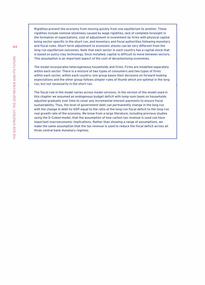
TH
E E
CB
ST
RA
TE
GY
: TH
E 2
02
1 R
EV
IEW
AN
D I
TS
FU
TU
RE
84
Rigidities prevent the economy from moving quickly from one equilibrium to another. These
rigidities include nominal stickiness caused by wage rigidities, lack of complete foresight in
the formation of expectations, cost of adjustment in investment by firms with physical capital
being sector-specific in the short run, and monetary and fiscal authorities following monetary
and fiscal rules. Short-term adjustment to economic shocks can be very different from the
long-run equilibrium outcomes. Note that each sector in each country has a capital stock that
is based on putty-clay technology. Once installed, capital is difficult to move between sectors.
This assumption is an important aspect of the cost of decarbonising economies.
The model incorporates heterogeneous households and firms. Firms are modelled separately
within each sector. There is a mixture of two types of consumers and two types of firms
within each sector, within each country: one group bases their decisions on forward-looking
expectations and the other group follows simpler rules of thumb which are optimal in the long
run, but not necessarily in the short run.
The fiscal rule in the model varies across model versions. In the version of the model used in
this chapter we assumed an endogenous budget deficit with lump-sum taxes on households
adjusted gradually over time to cover any incremental interest payments to ensure fiscal
sustainability. Thus, the level of government debt can permanently change in the long run
with the change in debt-to-GDP equal to the ratio of the long-run fiscal deficit to the long-run
real growth rate of the economy. We know from a large literature, including previous studies
using the G-Cubed model, that the assumption of how carbon tax revenue is used can have
important macroeconomic implications. Rather than showing a range of assumptions, we
make the same assumption that the tax revenue is used to reduce the fiscal deficit across all
three central bank monetary regimes.
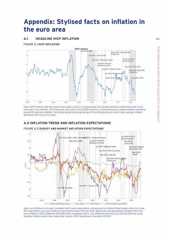
85
AP
PE
ND
Ix: S
Ty
LIS
ED
FA
CT
S O
N IN
FL
AT
ION
IN T
HE
EU
RO
AR
EA
Appendix: Stylised facts on inflation in the euro areaA.1 HEADLINE HICP INFLATION
FIGURE A.1 HICP INFLATION
2000 2002 2005 2007 2010 2012 2015 2017 2020-1
0
1
2
3
4
HICP inflationMay 2010: SMP
Dec 2011: 3-year LTRO
July 2012: "whatever it takes"
July 2013: Forwardguidance on rates
June 2014: Negative rates
Jan 2015: QE announced
March 2015: start QE
March 2016: QE expandedto 80bn/mo
Jun 2018: End ofQE announced
Dec 2018: End of QE
Sep 2019: Restart QEto 80bn/mo
Mar 2020: PEPP
Note: HICP inflation from the onset of the single currency to today shows two periods marked by differences both in the level and in the volatility. The first period, that lasts till the 2008 recession, is characterised by a stable inflation oscillating around 2% and low volatility. The second period sees large swings of the inflation process and a lower average inflation well below 2%. Source: Eurostat.
A.2 INFLATION TREND AND INFLATION ExPECTATIONS
FIGURE A.2 SURvEY AND MARKET INFLATION ExPECTATIONS
2006 2008 2010 2012 2014 2016 2018 2020
-0.5
0
0.5
1
1.5
2
2.5
3
3.5
4
YoY
%
Jul 2008: increase
Oct, Nov & Dec, 2008: decreases
May 2010: SMP
Dec 2011: 3-year LTRO
Jul 2012: "whatever it takes"Jul 2013: Forwardguidance on rates
Jun 2014: Negative rates
Jan 2015: QE announced
Mar 2015: start QE
Mar 2016: QE expanded
Jun 2018: End ofQE announced
Dec 2018: End of QE
Sep 2019: Restart
Mar 2020: PEPP
Inflation-linked Swap 5 Years Core inflation HICP inflation HICP 5Y-ahead forecast (SPF)
Note: core inflation is strongly correlated with 5-year expectations as measured by inflation-linked swaps while the 5-year SPF expectations are more stable but persistently below 2% since 2012. Notice also the gap between headline HICP and core inflation in 2007-2008 and 2011-2012 which suggested that in july 2008 and April and july 2011 the ECB was eying headline inflation rather than underlying. Source: ICAP (Datastream), Eurostat, ECB SPF.
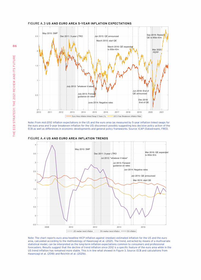
TH
E E
CB
ST
RA
TE
GY
: TH
E 2
02
1 R
EV
IEW
AN
D I
TS
FU
TU
RE
86
FIGURE A.3 US AND EURO AREA 5-YEAR INFLATION ExPECTATIONS
2010 2011 2012 2013 2014 2015 2016 2017 2018 2019 2020 20210
0.5
1
1.5
2
2.5May 2010: SMP
Dec 2011: 3-year LTRO
July 2012: "whatever it takes"
July 2013: Forwardguidance on rates
June 2014: Negative rates
Jan 2015: QE announced
March 2015: start QE
March 2016: QE expanded
Jun 2018: End ofQE announced
Dec 2018: End of QE
Sep 2019: Restart
Mar 2020: PEPP
Euro Area inflation-linked Swap 5 Years (%) US 5-Year Breakeven Inflation Rate
Note: From mid-2012 inflation expectations in the US and the euro area (as measured by 5-year inflation linked swaps for the euro area and 5-year breakeven inflation for the US) disconnect possibly suggesting less decisive policy action of the ECB as well as differences in economic developments and general policy frameworks. Source: ICAP (Datastream), FRED.
FIGURE A.4 US AND EURO AREA INFLATION TRENDS
2008 2010 2012 2014 2016-0.5
0
0.5
1
1.5
2
2.5
3
3.5
4
May 2010: SMP
Dec 2011: 3-year LTRO
Jul 2012: "whatever it takes"
Jul 2013: Forwardguidance on rates
Jun 2014: Negative rates
Jan 2015: QE announced
Mar 2015: start QE
Mar 2016: QE expanded
US median trend inflation EA median trend inflation EA inflation
Note: The chart reports euro area headline HICP inflation against (median) estimated inflation for the US and the euro area, calculated according to the methodology of Hasenzagl et al. (2021). The trend, extracted by means of a multivariate statistical model, can be interpreted as the long-term inflation expectations common to consumers and professional forecasters. Results suggest that the decline of trend inflation since 2012 is a specific feature of the euro area while in the US trend inflation has remained more stable. This is in line what showed in Figure 3. Source: ECB and calculations from Hasenzagl et al. (2018) and Reichlin et al. (2021b).
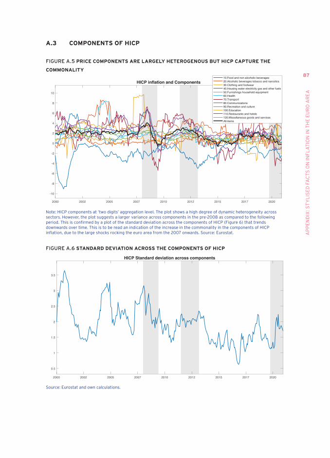
87
AP
PE
ND
Ix: S
Ty
LIS
ED
FA
CT
S O
N IN
FL
AT
ION
IN T
HE
EU
RO
AR
EA
A.3 COMPONENTS OF HICP
FIGURE A.5 PRICE COMPONENTS ARE LARGELY HETEROGENOUS BUT HICP CAPTURE THE
COMMONALITY
2000 2002 2005 2007 2010 2012 2015 2017 2020
-10
-8
-6
-4
-2
0
2
4
6
8
10
HICP inflation and Components10.Food and non-alcoholic beverages20.Alcoholic beverages tobacco and narcotics30.Clothing and footwear40.Housing water electricity gas and other fuels50.Furnishings household equipment60.Health70.Transport80.Communications90.Recreation and culture100.Education110.Restaurants and hotels120.Miscellaneous goods and servicesAll-items
Note: HICP components at ‘two digits’ aggregation level. The plot shows a high degree of dynamic heterogeneity across sectors. However, the plot suggests a larger variance across components in the pre-2008 as compared to the following period. This is confirmed by a plot of the standard deviation across the components of HICP (Figure 6) that trends downwards over time. This is to be read an indication of the increase in the commonality in the components of HICP inflation, due to the large shocks rocking the euro area from the 2007 onwards. Source: Eurostat.
FIGURE A.6 STANDARD DEvIATION ACROSS THE COMPONENTS OF HICP
2000 2002 2005 2007 2010 2012 2015 2017 2020
0.5
1
1.5
2
2.5
3
3.5
HICP Standard deviation across components
Source: Eurostat and own calculations.
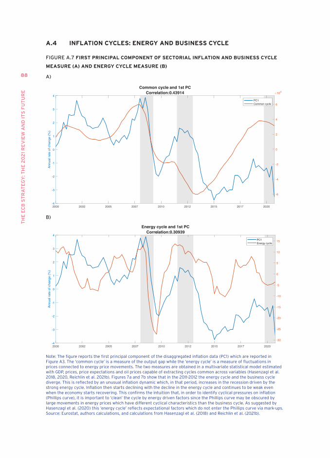
TH
E E
CB
ST
RA
TE
GY
: TH
E 2
02
1 R
EV
IEW
AN
D I
TS
FU
TU
RE
88
A.4 INFLATION CYCLES: ENERGY AND BUSINESS CYCLE
FIGURE A.7 FIRST PRINCIPAL COMPONENT OF SECTORIAL INFLATION AND BUSINESS CYCLE
MEASURE (A) AND ENERGY CYCLE MEASURE (B)
A)
2000 2002 2005 2007 2010 2012 2015 2017 2020-4
-3
-2
-1
0
1
2
3
4
Annu
al ra
te o
f cha
nge
(%)
-6
-4
-2
0
2
4
6
104Common cycle and 1st PC
Correlation:0.43914PC1Common cycle
B)
2000 2002 2005 2007 2010 2012 2015 2017 2020-4
-3
-2
-1
0
1
2
3
4
Annu
al ra
te o
f cha
nge
(%)
-30
-25
-20
-15
-10
-5
0
5
10
15
Energy cycle and 1st PCCorrelation:0.30939
PC1Energy cycle
Note: The figure reports the first principal component of the disaggregated inflation data (PC1) which are reported in Figure A3. The ‘common cycle’ is a measure of the output gap while the ‘energy cycle’ is a measure of fluctuations in prices connected to energy price movements. The two measures are obtained in a multivariate statistical model estimated with GDP, prices, price expectations and oil prices capable of extracting cycles common across variables (Hasenzagl et al. 2018, 2020, Reichlin et al. 2021b). Figures 7a and 7b show that in the 2011-2012 the energy cycle and the business cycle diverge. This is reflected by an unusual inflation dynamic which, in that period, increases in the recession driven by the strong energy cycle. Inflation then starts declining with the decline in the energy cycle and continues to be weak even when the economy starts recovering. This confirms the intuition that, in order to identify cyclical pressures on inflation (Phillips curve), it is important to ‘clean’ the cycle by energy driven factors since the Phillips curve may be obscured by large movements in energy prices which have different cyclical characteristics than the business cycle. As suggested by Hasenzagl et al. (2020) this ‘energy cycle’ reflects expectational factors which do not enter the Phillips curve via mark-ups. Source: Eurostat, authors calculations, and calculations from Hasenzagl et al. (2018) and Reichlin et al. (2021b).
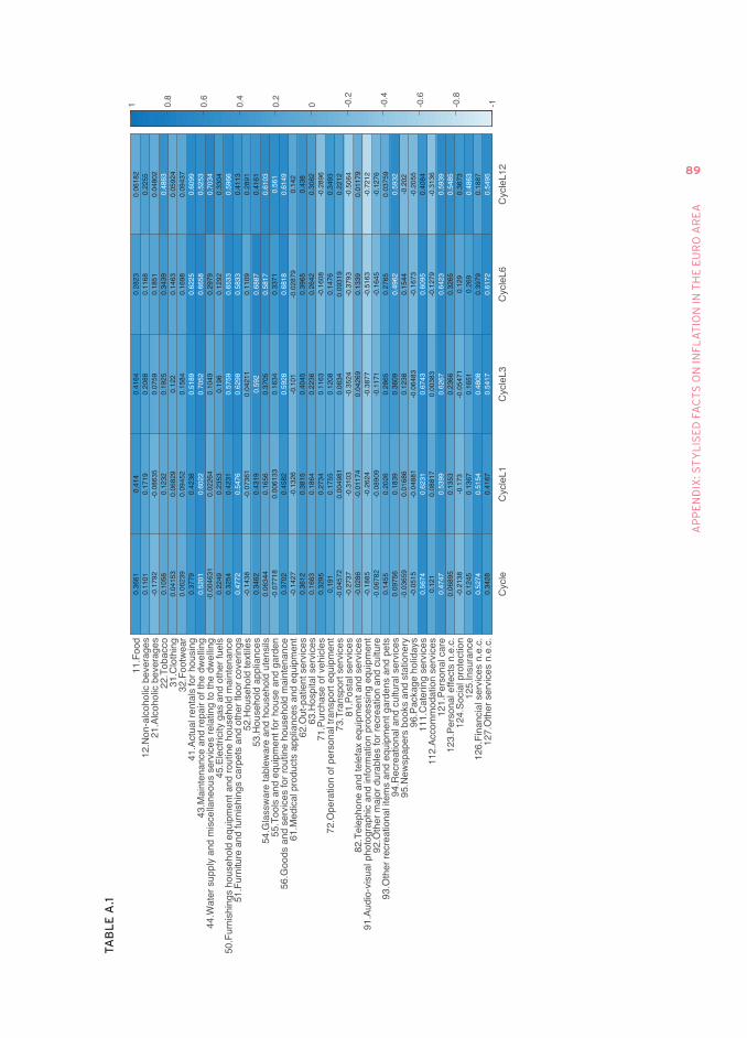
89
AP
PE
ND
Ix: S
Ty
LIS
ED
FA
CT
S O
N IN
FL
AT
ION
IN T
HE
EU
RO
AR
EA
TAB
LE
A.1
Cyc
leC
ycle
L1C
ycle
L3C
ycle
L6C
ycle
L12
11.F
ood
12.N
on-a
lcoh
olic
bev
erag
es21
.Alc
ohol
ic b
ever
ages
22.T
obac
co31
.Clo
thin
g32
.Foo
twea
r41
.Act
ual r
enta
ls fo
r hou
sing
43.M
aint
enan
ce a
nd re
pair
of th
e dw
ellin
g44
.Wat
er s
uppl
y an
d m
isce
llane
ous
serv
ices
rela
ting
to th
e dw
ellin
g45
.Ele
ctric
ity g
as a
nd o
ther
fuel
s50
.Fur
nish
ings
hou
seho
ld e
quip
men
t and
rout
ine
hous
ehol
d m
aint
enan
ce51
.Fur
nitu
re a
nd fu
rnis
hing
s ca
rpet
s an
d ot
her f
loor
cov
erin
gs52
.Hou
seho
ld te
xtile
s53
.Hou
seho
ld a
pplia
nces
54.G
lass
war
e ta
blew
are
and
hous
ehol
d ut
ensi
ls55
.Too
ls a
nd e
quip
men
t for
hou
se a
nd g
arde
n56
.Goo
ds a
nd s
ervi
ces
for r
outin
e ho
useh
old
mai
nten
ance
61.M
edic
al p
rodu
cts
appl
ianc
es a
nd e
quip
men
t62
.Out
-pat
ient
ser
vice
s63
.Hos
pita
l ser
vice
s71
.Pur
chas
e of
veh
icle
s72
.Ope
ratio
n of
per
sona
l tra
nspo
rt eq
uipm
ent
73.T
rans
port
serv
ices
81.P
osta
l ser
vice
s82
.Tel
epho
ne a
nd te
lefa
x eq
uipm
ent a
nd s
ervi
ces
91.A
udio
-vis
ual p
hoto
grap
hic
and
info
rmat
ion
proc
essi
ng e
quip
men
t92
.Oth
er m
ajor
dur
able
s fo
r rec
reat
ion
and
cultu
re93
.Oth
er re
crea
tiona
l ite
ms
and
equi
pmen
t gar
dens
and
pet
s94
.Rec
reat
iona
l and
cul
tura
l ser
vice
s95
.New
spap
ers
book
s an
d st
atio
nery
96.P
acka
ge h
olid
ays
111.
Cat
erin
g se
rvic
es11
2.Ac
com
mod
atio
n se
rvic
es12
1.Pe
rson
al c
are
123.
Pers
onal
effe
cts
n.e.
c.12
4.So
cial
pro
tect
ion
125.
Insu
ranc
e12
6.Fi
nanc
ial s
ervi
ces
n.e.
c.12
7.O
ther
ser
vice
s n.
e.c.
0.36
610.
1101
-0.1
792
0.10
560.
0415
30.
0623
90.
3779
-0.0
0463
10.
2249
0.32
54
-0.1
438
0.34
620.
0634
4-0
.077
180.
3702
-0.1
427
0.36
120.
1663
0.32
950.
191
-0.0
4572
-0.2
737
-0.0
286
-0.1
885
-0.0
6782
0.14
550.
0975
6-0
.036
59-0
.051
5
0.12
1
0.06
895
-0.2
138
0.12
45
0.34
28
0.41
40.
1719
-0.0
8635
0.12
320.
0682
90.
0945
20.
4238
0.02
264
0.23
530.
4231
-0.0
7361
0.43
190.
1656
0.00
6133
0.45
82-0
.132
60.
3815
0.18
640.
2734
0.17
550.
0049
81-0
.310
3-0
.011
74-0
.262
4-0
.089
090.
2026
0.18
390.
0168
6-0
.048
81
0.08
817
0.13
53-0
.173
0.13
67
0.41
67
0.41
640.
2088
0.07
590.
1925
0.12
20.
1584
0.10
490.
196
0.04
211
0.37
050.
1634
-0.1
010.
4045
0.22
360.
1163
0.12
080.
0634
-0.3
524
0.04
269
-0.3
877
-0.1
171
0.28
650.
3609
0.12
38-0
.064
83
0.00
383
0.23
66-0
.054
710.
1651
0.28
230.
1168
0.18
510.
3439
0.14
630.
1698
0.29
790.
1292
0.11
09
0.33
71
-0.0
2879
0.39
650.
2642
-0.1
608
0.14
760.
0931
9-0
.379
30.
1339
-0.5
163
-0.1
645
0.27
65
0.15
44-0
.167
3
-0.1
279
0.32
650.
129
0.26
90.
3979
0.06
182
0.22
550.
0480
2
0.05
924
0.09
437
0.33
04
0.41
130.
2891
0.41
61
0.14
20.
438
0.30
82-0
.289
60.
3493
0.22
12-0
.506
40.
0117
9-0
.721
2-0
.127
60.
0375
9
-0.2
02-0
.205
50.
4084
-0.3
136
0.36
73
0.18
87
0.52
01
0.47
72
0.56
74
0.47
47
0.52
74
0.60
22
0.54
76
0.62
31
0.53
99
0.51
54
0.51
890.
7052
0.57
590.
6298
0.59
2
0.59
28
0.67
43
0.62
67
0.48
080.
5417
0.62
250.
6658
0.65
330.
5833
0.68
870.
5817
0.68
18
0.49
62
0.60
95
0.64
23
0.61
72
0.48
63
0.60
990.
5253
0.70
34
0.59
66
0.61
030.
561
0.61
49
0.59
32
0.59
390.
5485
0.48
63
0.54
95-1-0
.8
-0.6
-0.4
-0.2
00.2
0.4
0.6
0.8
1
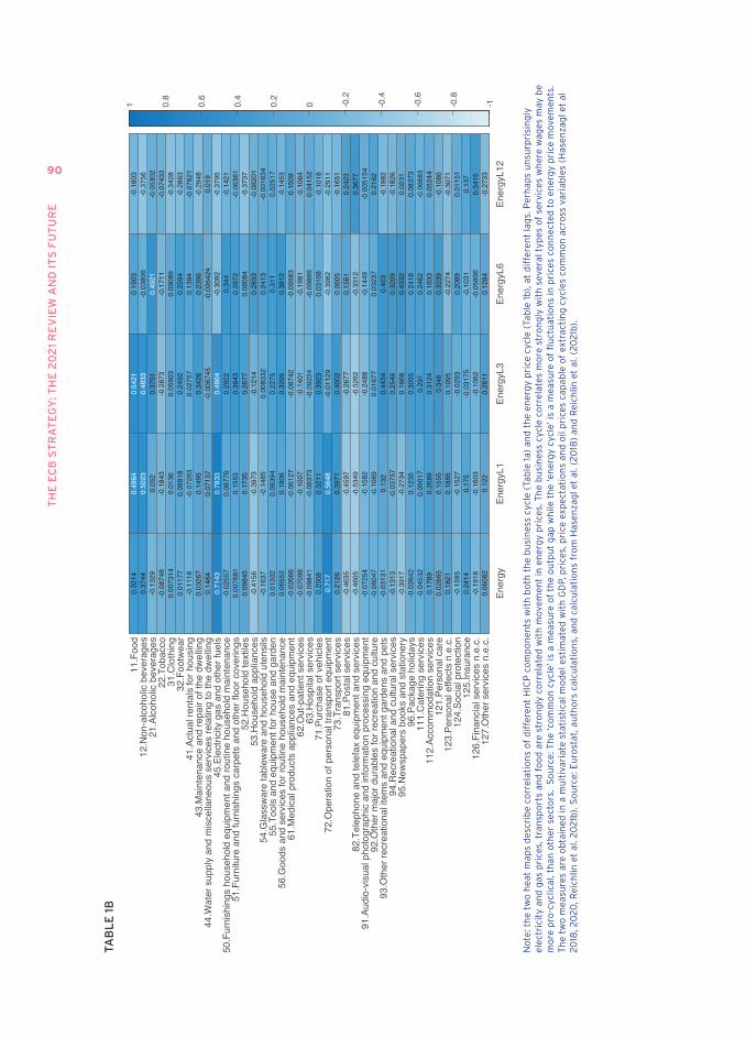
TH
E E
CB
ST
RA
TE
GY
: TH
E 2
02
1 R
EV
IEW
AN
D I
TS
FU
TU
RE
90
TAB
LE
1B
Ener
gyEn
ergy
L1En
ergy
L3En
ergy
L6En
ergy
L12
11.F
ood
12.N
on-a
lcoh
olic
bev
erag
es21
.Alc
ohol
ic b
ever
ages
22.T
obac
co31
.Clo
thin
g32
.Foo
twea
r41
.Act
ual r
enta
ls fo
r hou
sing
43.M
aint
enan
ce a
nd re
pair
of th
e dw
ellin
g44
.Wat
er s
uppl
y an
d m
isce
llane
ous
serv
ices
rela
ting
to th
e dw
ellin
g45
.Ele
ctric
ity g
as a
nd o
ther
fuel
s50
.Fur
nish
ings
hou
seho
ld e
quip
men
t and
rout
ine
hous
ehol
d m
aint
enan
ce51
.Fur
nitu
re a
nd fu
rnis
hing
s ca
rpet
s an
d ot
her f
loor
cov
erin
gs52
.Hou
seho
ld te
xtile
s53
.Hou
seho
ld a
pplia
nces
54.G
lass
war
e ta
blew
are
and
hous
ehol
d ut
ensi
ls55
.Too
ls a
nd e
quip
men
t for
hou
se a
nd g
arde
n56
.Goo
ds a
nd s
ervi
ces
for r
outin
e ho
useh
old
mai
nten
ance
61.M
edic
al p
rodu
cts
appl
ianc
es a
nd e
quip
men
t62
.Out
-pat
ient
ser
vice
s63
.Hos
pita
l ser
vice
s71
.Pur
chas
e of
veh
icle
s72
.Ope
ratio
n of
per
sona
l tra
nspo
rt eq
uipm
ent
73.T
rans
port
serv
ices
81.P
osta
l ser
vice
s82
.Tel
epho
ne a
nd te
lefa
x eq
uipm
ent a
nd s
ervi
ces
91.A
udio
-vis
ual p
hoto
grap
hic
and
info
rmat
ion
proc
essi
ng e
quip
men
t92
.Oth
er m
ajor
dur
able
s fo
r rec
reat
ion
and
cultu
re93
.Oth
er re
crea
tiona
l ite
ms
and
equi
pmen
t gar
dens
and
pet
s94
.Rec
reat
iona
l and
cul
tura
l ser
vice
s95
.New
spap
ers
book
s an
d st
atio
nery
96.P
acka
ge h
olid
ays
111.
Cat
erin
g se
rvic
es11
2.Ac
com
mod
atio
n se
rvic
es12
1.Pe
rson
al c
are
123.
Pers
onal
effe
cts
n.e.
c.12
4.So
cial
pro
tect
ion
125.
Insu
ranc
e12
6.Fi
nanc
ial s
ervi
ces
n.e.
c.12
7.O
ther
ser
vice
s n.
e.c.
0.32
140.
3744
-0.1
329
-0.0
8748
0.00
7314
0.01
177
-0.1
118
0.03
267
0.14
64
-0.0
2557
0.00
7681
0.09
845
-0.4
156
-0.1
637
0.01
302
0.06
552
-0.0
2666
-0.0
7098
-0.0
9841
0.23
08
0.21
26-0
.463
5-0
.460
5-0
.072
54-0
.060
47-0
.031
31-0
.131
3-0
.391
7-0
.026
42-0
.045
320.
1789
0.02
865
0.18
21-0
.159
50.
2414
-0.1
918
0.06
082
0.05
2-0
.184
30.
0136
0.08
818
-0.0
7263
0.14
950.
0713
7
0.08
776
0.15
530.
1735
-0.3
973
-0.1
465
0.08
394
0.18
06-0
.061
27-0
.100
7-0
.083
730.
3211
0.39
71-0
.459
7-0
.534
9-0
.158
2-0
.106
90.
132
-0.0
3757
-0.2
734
0.12
350.
0901
70.
2689
0.15
550.
1885
-0.1
527
0.17
5-0
.160
30.
122
0.37
51-0
.287
30.
0590
30.
2492
0.02
757
0.34
26-0
.008
745
0.29
220.
3643
0.26
77-0
.121
40.
0083
320.
2275
0.32
95-0
.087
42-0
.140
1-0
.092
240.
3923
-0.0
1129
0.40
02-0
.267
7-0
.526
2-0
.248
80.
0167
70.
4434
0.25
460.
1668
0.30
550.
291
0.31
240.
346
0.10
95-0
.029
3-0
.031
75-0
.106
20.
2611
0.19
03-0
.038
06
-0.1
711
0.09
089
0.25
940.
1394
0.23
96-0
.006
424
-0.3
092
0.34
40.
2872
0.08
084
0.28
330.
2413
0.31
10.
3812
-0.0
6983
-0.1
981
-0.0
9866
0.03
108
-0.3
982
0.06
050.
1561
-0.3
312
-0.1
449
0.03
237
0.40
30.
3209
0.43
320.
2418
0.24
620.
1633
0.32
39-0
.227
40.
2089
-0.1
031
-0.0
5806
0.12
84
-0.1
803
-0.3
756
-0.0
5302
-0.0
7433
-0.3
428
-0.2
863
-0.0
7621
-0.2
948
0.01
9-0
.379
5-0
.142
1-0
.063
61-0
.373
7-0
.082
01-0
.001
634
0.02
517
-0.1
453
0.15
09-0
.106
40.
0415
2-0
.101
8-0
.291
1-0
.165
10.
2423
0.36
77-0
.005
154
0.21
62-0
.198
2-0
.182
60.
0231
0.08
373
-0.0
6683
0.05
244
-0.1
086
-0.3
071
0.01
151
0.13
70.
3415
-0.2
733
0.71
43
0.71
7
0.49
640.
5023
0.78
33
0.56
48
0.54
210.
4833
0.48
64
0.49
21
-1-0.8
-0.6
-0.4
-0.2
00.2
0.4
0.6
0.8
1
No
te: t
he
two
hea
t m
aps
des
crib
e co
rrel
atio
ns
of
dif
fere
nt
HIC
P c
om
po
nen
ts w
ith
bo
th t
he
bu
sin
ess
cycl
e (T
able
1a)
an
d t
he
ener
gy
pri
ce c
ycle
(Ta
ble
1b)
, at
dif
fere
nt
lag
s. P
erh
aps
un
surp
risi
ng
ly
elec
tric
ity
and
gas
pri
ces,
tra
nsp
ort
s an
d f
oo
d a
re s
tro
ng
ly c
orr
elat
ed w
ith
mov
emen
t in
en
erg
y p
rice
s. T
he
bu
sin
ess
cycl
e co
rrel
ates
mo
re s
tro
ng
ly w
ith
sev
eral
typ
es o
f se
rvic
es w
her
e w
ages
may
be
mo
re p
ro-c
yclic
al, t
han
oth
er s
ecto
rs.
So
urc
e: T
he
‘co
mm
on
cyc
le’ i
s a
mea
sure
of
the
ou
tpu
t g
ap w
hile
th
e ‘e
ner
gy
cycl
e’ is
a m
easu
re o
f fl
uct
uat
ion
s in
pri
ces
con
nec
ted
to
en
erg
y p
rice
mov
emen
ts.
Th
e tw
o m
easu
res
are
ob
tain
ed in
a m
ult
ivar
iate
sta
tist
ical
mo
del
est
imat
ed w
ith
GD
P, p
rice
s, p
rice
exp
ecta
tio
ns
and
oil
pri
ces
cap
able
of
extr
acti
ng
cyc
les
com
mo
n a
cro
ss v
aria
ble
s (H
asen
zag
l et
al
20
18, 2
02
0, R
eich
lin e
t al
. 20
21b
). S
ou
rce:
Eu
rost
at, a
uth
ors
cal
cula
tio
ns,
an
d c
alcu
lati
on
s fr
om
Has
enza
gl e
t al
. (2
018
) an
d R
eich
lin e
t al
. (2
02
1b).
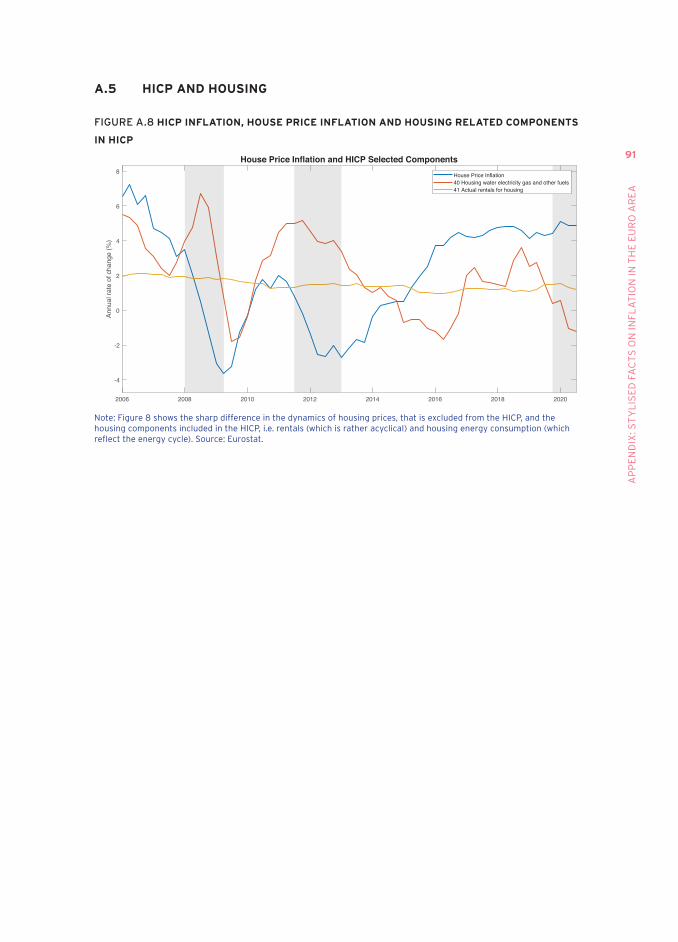
91
AP
PE
ND
Ix: S
Ty
LIS
ED
FA
CT
S O
N IN
FL
AT
ION
IN T
HE
EU
RO
AR
EA
A.5 HICP AND HOUSING
FIGURE A.8 HICP INFLATION, HOUSE PRICE INFLATION AND HOUSING RELATED COMPONENTS
IN HICP
2006 2008 2010 2012 2014 2016 2018 2020
-4
-2
0
2
4
6
8
Annu
al ra
te o
f cha
nge
(%)
House Price Inflation and HICP Selected ComponentsHouse Price Inflation40 Housing water electricity gas and other fuels41 Actual rentals for housing
Note: Figure 8 shows the sharp difference in the dynamics of housing prices, that is excluded from the HICP, and the housing components included in the HICP, i.e. rentals (which is rather acyclical) and housing energy consumption (which reflect the energy cycle). Source: Eurostat.
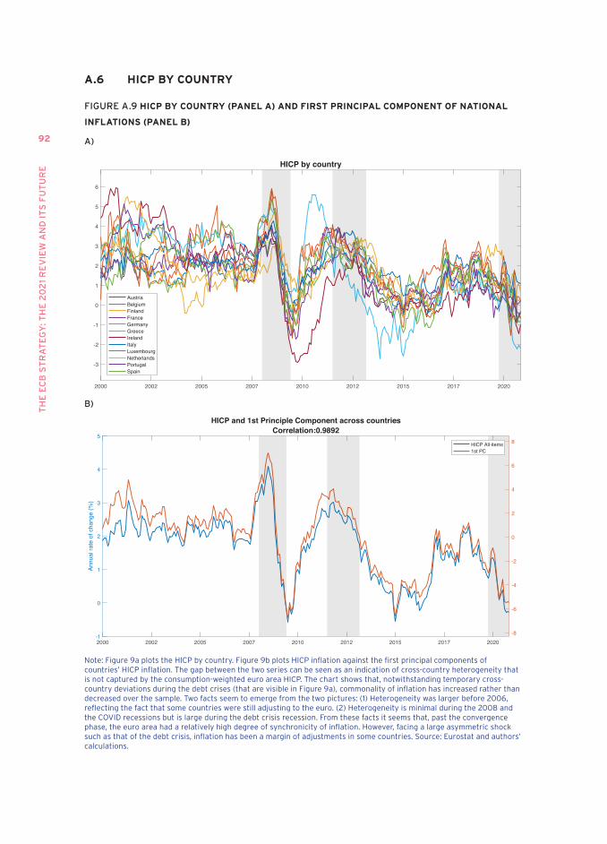
TH
E E
CB
ST
RA
TE
GY
: TH
E 2
02
1 R
EV
IEW
AN
D I
TS
FU
TU
RE
92
A.6 HICP BY COUNTRY
FIGURE A.9 HICP BY COUNTRY (PANEL A) AND FIRST PRINCIPAL COMPONENT OF NATIONAL
INFLATIONS (PANEL B)
A)
2000 2002 2005 2007 2010 2012 2015 2017 2020
-3
-2
-1
0
1
2
3
4
5
6
HICP by country
AustriaBelgiumFinlandFranceGermanyGreeceIrelandItalyLuxembourgNetherlandsPortugalSpain
B)
2000 2002 2005 2007 2010 2012 2015 2017 2020-1
0
1
2
3
4
5
Annu
al ra
te o
f cha
nge
(%)
-8
-6
-4
-2
0
2
4
6
8
HICP and 1st Principle Component across countriesCorrelation:0.9892
HICP All-items1st PC
Note: Figure 9a plots the HICP by country. Figure 9b plots HICP inflation against the first principal components of countries’ HICP inflation. The gap between the two series can be seen as an indication of cross-country heterogeneity that is not captured by the consumption-weighted euro area HICP. The chart shows that, notwithstanding temporary cross-country deviations during the debt crises (that are visible in Figure 9a), commonality of inflation has increased rather than decreased over the sample. Two facts seem to emerge from the two pictures: (1) Heterogeneity was larger before 2006, reflecting the fact that some countries were still adjusting to the euro. (2) Heterogeneity is minimal during the 2008 and the COVID recessions but is large during the debt crisis recession. From these facts it seems that, past the convergence phase, the euro area had a relatively high degree of synchronicity of inflation. However, facing a large asymmetric shock such as that of the debt crisis, inflation has been a margin of adjustments in some countries. Source: Eurostat and authors’ calculations.
93
RE
FE
RE
NC
ES
ReferencesAbadie, A and J Gardeazabal (2003), “The economic cost of conflict: A case study of the Basque Country”, American Economic Review 93(1): 113-132.
Adam, K (2021), “Monetary Policy Challenges from Falling Natural Rates of Interest”, Proceedings of the 2020 ECB Forum on Central Banking, pp. 186-209.
Adam, K and R Billi (2006), “Optimal Monetary Policy under Commitment with a Zero Bound on Nominal Interest Rates”, Journal of Money, Credit and Banking 38(7): 1877-1905.
Adam, K and P Tzamourani (2016), “Distributional Consequences of Asset Price Inflation in the Euro Area”, European Economic Review 89: 172–192.
Adam, K and H Weber (2019), “Optimal Trend Inflation”, American Economic Review 109(2): 702-737.
Adam, K and H Weber (2020), “Estimating the Optimal Inflation Target from Trends in Relative Prices”, CEPR Discussion Paper 14335.
Adam, K, O Pfaeuti, and Z Reinelt (2020), “Falling Natural Rates, Rising Housing Volatility and the Optimal Inflation Target”, CRC TR 224 Discussion Paper 235.
Adam, K, E Gautier, S Santoro and H Weber (2021), “The Case for a Positive Inflation Target in the Euro Area: Evidence from France, Germany and Italy”, ECB Working Paper 2575.
Alexandrov, A (2020), “The Effects of Trend Inflation on Aggregate Dynamics and Monetary Stabilization”, CRC TR 224 Discussion Paper 216.
Alesina, A and A Stella (2010), “The Politics of Monetary Policy”, Chapter 18 in B M Friedman and M Woodford (eds), Handbook of Monetary Economics, Volume 3, 1st edition, Elsevier.
Altavilla, C, L Brugnolini, R Gürkaynak, R Motto and G Ragusa (2019), “Measuring euro area monetary policy”, Journal of Monetary Economics 108(C): 162-179.
Alvarez, F, M Beraja, M Gonzalez-Rozada, P A Neumeyer (2018), “Form Hyperinflation to Stable Prices. Argentina’s Evidence on Menu Cost Models”, Quarterly Journal of Economics 134: 451-505.
Andrade, P, J Galì, H Le Bihan, J Matheron (2019), “The Optimal Inflation Target and the Natural Rate of Interest”, Brookings Papers on Economic Activity, Fall.
Bartsch, E, A Bénassy-Quéré, G Corsetti, and X Debrun (2020), It’s all in the mix: How can monetary and fiscal policies work or fail together?, Geneva Report on the World Economy No 23, ICMB and CEPR.
TH
E E
CB
ST
RA
TE
GY
: TH
E 2
02
1 R
EV
IEW
AN
D I
TS
FU
TU
RE
94
Bassetto, M and T J Sargent (2020), “Shotgun Wedding: Fiscal and Monetary Policy”, Annual Review of Economics 12(1).
Benigno, P and S Nisticò (2020), “Non-neutrality of Open-Market Operations”, American Economic Journal: Macroeconomics 12(3): 175-226.
Bernard, J-T, M Kichian and M Islam (2018), “Effects of BC’s Carbon Tax on GDP.” USAEE Research Paper Series No. 18-329.
Bhattarai, S, G B Eggertsson and B Gafarov (2021), “Time Consistency and the Duration of Government Debt: A Signalling Theory of Quantitative Easing”, NBER Working Paper No. 21336.
Blanco, A (2021), “The Optimal Inflation Target in an Economy with Menu Costs and Zero Lower Bound”, American Economic Journal: Macroeconomics 13(3): 108-141.
Bocola, L, and A Dovis (2019), “Self-Fulfilling Debt Crises: A Quantitative Analysis”, American Economic Review 109 (12): 4343-77.
Brand, C and F Mazelis (2019), “Taylor-rule Consistent Estimates of the Natural Rate of Interest”, ECB Working Paper 2257.
Brunnermeier, M (2020), “Fiscal and Financial Dominance 2nd Pillar: Trap Analysis”, ECB Sintra Forum Intervention.
Castillo-Martínez, L and R Reis (2019), “How do central banks control inflation? A guide for the perplexed”, mimeo.
CfM – Centre for Macroeconomics (2021), “CfM Survey: The ECB’s Green Agenda”.
Cochrane, J H (2019), “The fiscal roots of inflation”, NBER Technical.
Cochrane, J H (2020), “The Fiscal Theory of the Price Level”, unpublished.
Coibion, O, Y Gorodnichenko and J Wieland (2012), “The Optimal Inflation Rate in New Keynesian Models: Should Central Bank Raise Their Inflation Targets in Light of the Zero Lower Bound?”, Review of Economic Studies 79: 1371-1406.
Coibion, O, Y Gorodnichenko, E S Knotek II and R Schoenle (2020), “Average Inflation Targeting and Household Expectations”, CEPR Discussion Paper 15307.
Colangelo, A, D Giannone, M Lenza, H Pill, Huw and L Reichlin(2017), “The national segmentation of euro area bank balance sheets during the financial crisis”, Empirical Economics 53(1): 247-265.
Corsetti, G and L Dedola (2016), “The mystery of the printing press: Self- fulfilling debt crises and monetary sovereignty”, Journal of the European Economic Association 14(6): 1329–1371.
95
RE
FE
RE
NC
ES
Dell’Ariccia, G, P Rabanal and D Sandri (2018), “Unconventional Monetary Policies in the Euro Area, Japan, and the United Kingdom”, Journal of Economic Perspectives 32(4): 147-72.
Del Negro, M and C A Sims (2015), “When does a central bank׳s balance sheet require fiscal support?”, Journal of Monetary Economics 73(C): 1-19.
Draghi, M (2014), “Unemployment in the euro area”, speech at the Annual Central Bank Symposium in Jackson Hole, 22 August.
Eggertsson, G and M Woodford (2003), “The Zero Interest-Bound and Optimal Monetary Policy”, Brookings Papers on Economic Activity 1: 139-211.
Ens, E and C Johnston (2020), “Scenario Analysis and the Economic and Financial Risks from Climate Change”, Bank of Canada Staff Discussion Paper 2020-3.
Giannone, G, M Lenza, H Pill and L Reichlin (2012), “The ECB and the Interbank Market”, Economic Journal 122(564): 467-486.
Gilchrist, S and B Mojon (2018), “Credit Risk in the Euro Area”, Economic Journal 128: 118-158.
Greenwood, R, S G Hanson, J S Rudolph and L Summers (2015),”Debt Management Conflicts between the U.S. Treasury and the Federal Reserve”, in D Wessel (ed.), The $13 Trillion Question: How America Manages Its Debt, Brookings Institution Press.
Hall, R E and R Reis (2015), “Maintaining Central-Bank Financial Stability under New-Style Central Banking”, NBER Working Paper No. 21173.
Hartman, P and F Smets (2018), “The European Central Bank’s Monetary Policy during Its First 20 Years”, Brookings Papers on Economic Activity 49(2): 1-146.
Hasenzagl, T, F Pellegrino, L Reichlin and G Ricco (2018), “Low inflation for longer”, VoxEUorg, 15 January.
Hasenzagl, T, F Pellegrino, L Reichlin and G Ricco (2020), “A Model of the Fed›s View on Inflation”, The Review of Economics and Statistics.
Henderson, D W and W McKibbin (1993), “A Comparison of Some Basic Monetary Policy Regimes for Open Economies: Implications of Different Degrees of Instrument Adjustment and Wage Persistence”, Carnegie-Rochester Conference Series on Public Policy 39: 221-318.
IMF – International Monetary Fund (2020), World Economic Outlook, October, Washington DC.
James, H (2012), Making the European Monetary Union, Belknap Press of Harvard University Press.
TH
E E
CB
ST
RA
TE
GY
: TH
E 2
02
1 R
EV
IEW
AN
D I
TS
FU
TU
RE
96
Jaumotte, F, W Liu, and W J McKibbin (2021), “Mitigating Climate Change: Growth-friendly Policies to Achieve Net Zero Emissions by 2050”, CAMA Working Paper, Australian National University.
Khan, A, R G King and A L Wolman (2003), “Optimal Monetary Policy”, Review of Economic Studies 70(4): 825-860.
Konradt, M and B Weder di Mauro (2021), “Carbon Taxation and Inflation: Evidence from the European and Canadian Experience”, CEPR Discussion Paper No. 16396.
Kremer, M, M Lo Duca and D Holló (2012), “CISS - a composite indicator of systemic stress in the financial system”, ECB Working Paper Series 1426.
Kydland, F E and E C Prescott (1977), “Rules Rather Than Discretion: The Inconsistency of Optimal Plans”, Journal of Political Economy 85: 473-492.
Lagarde, C (2020), “Climate change and the financial sector”, speech at the launch of the COP 26 Private Finance Agenda, London, 27 February.
Leeper, E M and C Leith (2016), “Understanding Inflation as a Joint Monetary-Fiscal Phenomenon”, in J B Taylor and H Uhlig (eds), Handbook of Macroeconomics, Volume 2, Elsevier.
L’Huillier, J P and R Schoenle (2020), “Raising the Inflation Target: How Much Extra Room Does It Really Give?”, Federal Reserve Bank of of Cleveland Working Paper 20-16.
Lorenzoni, G and I Werning (2019), “Slow Moving Debt Crises”, American Economic Review 109(9): 3229-63.
Mersch, Y (2014), “Monetary Policy and Economic Inequality”, speech at the Corporate Credit Conference, Zurich, 17 October.
Metcalf, G E (2019), “On the Economics of a Carbon Tax in the United States”, Brookings Papers on Economic Activity, Spring: 405-458.
Metcalf, G E and J H Stock (2020), “Measuring the macroeconomic impact of carbon taxes”, AEA Papers and Proceedings 110: 101-106.
McKibbin W and P Wilcoxen (2013), “A Global Approach to Energy and the Environment: The G-cubed Model”, Chapter 17 in Handbook of CGE Modeling, North Holland.
McKibbin W J, A Morris, P J Wilcoxen and A Panton (2020), “Climate change and monetary policy: Issues for policy design and modelling”, Oxford Review of Economic Policy 36(3): 579–603.
Miranda-Agrippino, S, and G Ricco (2021), “The Transmission of Monetary Policy Shocks”, American Economic Journal: Macroeconomics 13(3): 74-107.
Murray, B and N Rivers (2015), “British Columbia’s revenue-neutral carbon tax: A review of the latest ‘grand experiment’ in environmental policy”, Energy Policy 86: 674-683.
97
RE
FE
RE
NC
ES
NGFS – Central Banks and Supervisors Network for Greening the Financial System (2020), Progress report on the implementation of sustainable and responsible investment practices in central banks’ portfolio management, December.
NGFS (2021), Adapting Central Bank Operations to a Hotter World, March.
Orphanides, A and V Wieland (2013), “Complexity and Monetary Policy”, International Journal of Central Banking 9: 167-203.
Papoutsi, M, M Piazzesi, and M Schneider (2021), “How unconventional is green monetary policy?”, JEEA-FBBVA Lecture at ASSA, working paper.
Pill, H and L Reichlin (2015), “Exceptional policies for exceptional times The ECB’s response to the rolling crises of the euro area”, in Routledge Handbook of the Economics of European Integration.
Pill, H and L Reichlin (2017), “Non-Standard Monetary Policy and Financial Stability: Developing an Appropriate Macrofinancial Policy Mix”, in E Jokivuolle and R Tunaru (eds), Preparing for the Next Financial Crisis: Policies, Tools and Models, Cambridge University Press.
Rafaty, R, G Dolphin and F Pretis (2020), “Carbon pricing and the elasticity of CO2 emissions”, Institute for New Economic Thinking Working Paper No. 140.
Reichlin, L (2014), “Monetary Policy and Banks in the Euro Area: The Tale of Two Crises”, Journal of Macroeconomics 39(PB): 387-400.
Reichlin, L (2019), “La Banque Centrale Européenne et la Crise de l’Euro”, Fayard Paris, September.
Reichlin, L (2021), “Non-standard monetary policy instruments: effectiveness and risks”, in Central banks in a shifting world, Conference proceedings of the ECB Forum on Central Banking, Sintra 11-12 November.
Reichlin, L, A Turner and M Woodford (2013), “ Helicopter money as a policy option”, VoxEU.org, 23 September.
Reichlin, L, G Ricco, and M Tarbé (2021a), “Monetary-Fiscal Crosswinds in the European Monetary Union”, CEPR Discussion Paper 16138.
Reichlin, L, G Ricco and M Tarbé (2021b), “Inflation in the medium and long run in the Euro Area”, mimeo.
Reichlin, L, G Ricco and A Tuteja (2021c) “Monetary Policy Signals and Shocks in the Euro Area”, mimeo, London Business School.
Reis, R (2017), “QE in the Future: The Central Bank’s Balance Sheet in a Fiscal Crisis,” IMF Economic Review 65(1): 71-112.
TH
E E
CB
ST
RA
TE
GY
: TH
E 2
02
1 R
EV
IEW
AN
D I
TS
FU
TU
RE
98
Reis, R (2019), “Can the Central Bank Alleviate Fiscal Burdens?”, in D G Mayes, P L Siklos, and J-E Sturm (eds), The Oxford Handbook of the Economics of Central Banking, Oxford University Press.
Rostagno, M, C Altavilla, G Carboni, W Lemke, R Motto, A Saint Guilhem and J Yiangou (2019), “A tale of two decades: the ECB’s monetary policy at 20”, ECB Working Paper Series 2346.
Schmitt-Grohé, S and M Uribe (2020), “The Optimal Rate of Inflation”, Chapter 13 in B M Friedman and M Woodford (eds), Handbook of Monetary Economics, Volume 3.
Schnabel, I (2020), “When markets fail – the need for collective action in tackling climate change”, ECB speech, 28 September.
Schnabel, I (2021), “From green neglect to green dominance?”, comment at the “Greening Monetary Policy – Central Banking and Climate Change” online seminar, 3 March.
Taylor, J B (1993), “Discretion versus Policy Rules in Practice”, Carnegie-Rochester Series on Public Policy 39: 195-214.
Wallace, N (1981), “A Modigliani-Miller Theorem for Open-Market Operations”, American Economic Review 71(3): 267–274.
Woodford, M (1999), “Optimal Monetary Policy Inertia”, Manchester School 67: 1-35.
Woodford, M (2003), Interest and Prices, Princeton University Press.
Woodford, M (2012), “Methods of policy accommodation at the interest-rate lower bound”, Proceedings - Economic Policy Symposium - Jackson Hole, Federal Reserve Bank of Kansas City: 185-288.
Yamazaki, A (2017), “Jobs and Climate Policy: Evidence from British Columbia’s Revenue-Neutral Carbon Tax”, Journal of Environmental Economics and Management 83: 197-216.
33 Great Sutton Street | LONDON EC1V 0DX | UK
TEL: +44 (0)20 7183 8801 | FAX: +44 (0)20 7183 8820
EMAIL: [email protected]
WWW.CEPR.ORG9 781912 179497
ISBN 978-1-912179-49-7
ISBN: 978-1-912179-49-7
The European Central Bank recently completed an eighteen-month strategy review, published in July 2021, with the aim of innovating on both the design and the magnitude of its policy responses. This report, authored by senior European economists and written in parallel to the official review, provides a timely and clear framework to assess the current changes to and future evolution of the ECB’s strategy.
The report provides a structured discussion of four important topics which were part of the ECB’s analysis in the run up to its 2021 strategy review: the definition of the target (price stability and secondary objectives); the operational framework; fiscal-monetary policy interactions; and the implications for monetary policy of climate change and related mitigation initiatives.
The overall consensus is that the ECB is moving in a sensible direction, but many questions remain unanswered and it remains to be seen whether the new monetary policy strategy will successfully accommodate the challenges it has set out to meet. This report provides an excellent analytical accompaniment that will help frame the discussion going forward.