THE DUAL METHOD VIA THE ENVELOPE THEOREM FOR

SENSITIVITY ANALYSIS AND LE CHATELIER PRINCIPLE IN

PARAMETRIC OPTIMIZATION PROBLEMS

by

Emmanuel Drandakis Professor of Economics, Emeritus,

Athens University of Economics and Business Abstract The paper develops the dual method, via the Envelope theorem, for sensitivity analysis and Le Chatelier Principle in general parametric optimization problem. A unified approach in matrix theoretic methods is exhibited that relies, not only on envelope tangencies, but mainly on curvature conditions of appropriate envelope problems suitable for each purpose. If all parameters appear in all functions of the original problem then, no matter whether the associated envelope problem is constrained or not, curvature conditions are subject to constraints and cannot be used for either purpose; difficulties however are easily overcome by designing suitable representations of them that hold in the respective tangent subspaces. With a less general but more conducive parameter structure, unconstrained envelope problems lead directly to desired results. The dual method is as elegant and simple as the primal method of sensitivity analysis and Le Chatelier Principle in matrix terms. All basic results are obtained equally well; the same difficulties appear and are similarly dealt with. Finally, an economic application in the theory of consumer choice, without and with quantity rationing constraints, shows that the proposed dual method derives all known sensitivity results without any outside help. More importantly, it derives a richer vista of Le Chatelier effects, a feature due to more specific relationships between some parameters and some choice variables. Keywords: Envelope tangencies and curvature conditions, Dual and Primal method for Sensitivity analysis and Le Chatelier principle. JEL Classification: C 61

1

1. Introduction

In a recent paper – Drandakis (2003) – we considered Caratheodory΄s (1935)

theorem on the properties of the Inverse of the Bordered Hessian matrix of a general

constrained optimization problem. After a proof of the theorem, in matrix theoretic

terms, we proved a second theorem that compares the submatrices on the main

diagonal of the Inverse matrix, before and after new and “just binding” constraints are

introduced to the problem. Both theorems are instrumental in the Primal method of

comparative statics for examining the sensitivity of the optimal solution and Le

Chatelier Principle, as parameters of the problem vary.

The present paper focuses on the Dual method of sensitivity analysis, via the

Envelope Theorem, in which parameters of the original problem become the choice

variables while the former choice variables are treated as parameters. The first

Envelope problem compares the value of the objective function, at the fixed optimal

solution, to that of the optimal value function of the original problem, while the

second compares the optimal value functions of both problems after and before the

introduction of new constraints. The second-order conditions of both Envelope

problems furnish the curvature conditions needed for sensitivity analysis and Le

Chaterlier Principle.

Our aim is to produce a simple and unified formulation of the dual method that

was originally presented in the two basic papers of Silberberg and Hatta. Silberberg

(1974) examined a general constrained optimization problem, in which all parameters

appear in both the objective and constraint functions. Although only the first

Envelope problem is a constrained one, both problems lead to second-order conditions

specifying that a certain matrix of the rates of change of the optimal solution(s) must

be semi-definite, or definite on the tangent subspace. To use these restrictions for

our purposes, we must specify a matrix representation of the second-order

conditions in the tangent subspace, evaluate the matrix using the second-order

derivative properties of the optimal value functions and simplify it as much as

possible, so that the meaning of its semi-definiteness or definiteness becomes

transparent. Hatta (1980), on the other hand, examines a similar but less general

optimization problem in which, except for parameters appearing in the objective and

2

constraint functions, constraint levels are not constant but may also vary. Here the

first Envelope problem may be either a constrained one, needing a matrix

representation in the tangent subspace, or an unconstrained problem leading directly

to a semi-definite or definite matrix of the rates of change of the optimal solution.

When new and just binding constraints are introduced, the second Envelope problem

produces all desired results.

The paper is organized as follows. Section 2 considers the Silberberg and Hatta

models and the dual method via the Envelope Theorem, while Section 3 presents Le

Chatelier Principle for both models. Section 4 compares the basic features of the dual

and primal methods, while Section 5 presents a simple but important economic

application in the theory of consumer choice. There, the problems referred to in the

previous paragraph have led to the use of an indirect dual method, which borrows

relevant properties from a related optimization problem, the expenditure minimization

problem. Our dual method needs no outside help and shows that both utility

maximization and expenditure minimization can be used for proving sensitivity

results in the other problem. Finally concluding remarks and references are given in

Section 6.

Our analysis relies on classical optimization techniques in matrix theory terms. All

vectors are treated as column vectors, unless they are enclosed within parentheses or

appear as function arguments, while matrices are denoted by capital letters. Thus e.g.

0, 0m, or Omκ, indicate the zero scolar, a vector of m zeros, or an m x κ matrix of

zeros, respectively, while nix ( ) R and x( ) Rα ∈ α ∈ need no explanation, but Xα

(α) denotes the n x κ matrix of the partial derivatives of xi (α) in αj, i = 1, … , n

and j = 1, …, κ. Finally, a prime after a vector or a matrix denotes transposition.

2. The dual method of comparative statics via the Envelope Theorem

(a) The Silberberg model

Silberberg examines the problem

{ mx( ) max f (x, ) h(x, ) 0 }′ ′φ α ≡ α α = , (S)

3

where nx X R , A Rκ∈ ⊂ α∈ ⊂ and both X, A are open sets. The real-valued functions i 2f , h C , i 1,...,m ,∈ = with fx (x, α) , fα (x, α) and i i

xh (x, ) , h (x, )αα α their gradient

vectors and with Hx (x, α), Hα (x, α) denoting the m x n and m x κ gradient matrices

of h (x, α) in x and α, respectively. Finally the dimensionality restrictions

1 m n or=< < κ are imposed to ensure the feasibility of (S) and of problem c

S(E )

below. A feasible solution of (S) is regular if

r (Hx (x, α)) = m. (Rx)

(S) is well behaved having interior solutions. If x0 is regular and a local maximum of

(S), there exist lagrangean multipliers 0 0 01 m( ,..., )′λ ≡ λ λ and we have the necessary

conditions: m

0 0 i 0 0 0 0x i x x n

i 1f o c f (x , ) h (x , ) H (x , ) , h(x , ) 0

=

⎧ ⎫′− − α = λ α ≡ α λ α =⎨ ⎬

⎩ ⎭∑ (1)

and

0 0The hessian of (S) at x , is negatives o n c

semidefinite on the tan gent subspace

⎧ ⎫λ⎪ ⎪− − − ⎨ ⎬⎪ ⎪⎩ ⎭

. (2)

The hessian matrix is given by Fxx (x, α) – Hxx (x, λ. α), where m

ixx i xx

i 1H (x, , ) H (x, )

=

λ α ≡ λ α∑ is the sum of the matrices of second derivatives of

all hi (x, α) in x , weighted by their respective lagrangean multipliers1. The tangent

subspace at a regular x0 is given by { }n 0x mT R H (x , ) 0 .= η∈ α η= On the other

hand, if x0, λ0 satisfy (1) and if the

0 0 0

xx xx

n 0x m n

F (x , ) H (x , , ) is negative definites o s c

on{ R H (x , ) 0 , 0 }

⎧ ⎫α − λ α⎪ ⎪− − − ⎨ ⎬⎪ ⎪η∈ α η = η ≠⎩ ⎭

(2΄)

are also satisfied, then x0 attains a strict local maximum of (S). Finally, the Jacobian

of (1) in x and –λ,

1 The difference between the n x n Hxx (x, λ, α) and the m x n gradient matrix Hx (x, α) should be noted.

4

xx xx x

x mm mm

F (x, ) H (x, , ) , H (x, ) A , BH (x, ), O B , O

′α − λ α α⎡ ⎤ ⎡ ⎤≡⎢ ⎥ ⎢ ⎥′α⎣ ⎦ ⎣ ⎦

(3)

is the bordered Hessian of (S), which is an invertible matrix at a regular x0 that

satisfies (1) and (2΄)2. Then the Implicit function theorem works and the solution

vectors x(α), λ(α) are differentiable functions of Aα∈ 3 .

(b) Derivative properties of the maximal value function

We can easily see that

φα (α) = fα (x (α), α) – Ηα(x (α), α)΄ λ(α) , (4)

if we use (1) and differentiate the constraints. We will also need the second-order

derivative properties, which involve the symmetric matrix

x x( ) [F (x( ) , ) H (x( ) , ( ) , )]X ( )

[F (x( ) , ) H (x( ) , ( ) , )]

H (x( ) , ) ( )

αα α α α

αα αα

α α

Φ α = α α − α λ α α α +

+ α α − α λ α α −

′− α α Λ α

(5)

and are rarely mentioned in the literature. Here again n

ix i x

i 1H (x( ) , ( ), ) ( ) H (x( ), )α α

=

α λ α α = λ α α α∑ and similarly for H (x( ), ( ), )αα α λ α α .

(c) First Envelope problem for (S)

With parameter values at α0 , let x0 ≡ x (α0) , λ0 ≡ λ(α0). Can we compare the

difference, f (x0, α) – φ (α), of the value of the objective of (S) at x0 from the

maximal value function, as parameters vary around α0 ? The answer is no, despite

the facts that f (x0, α0) = φ (α0) and that φ (α) is the maximal value function of (S).

The reason is that, f(x0, α) as a function of Aα∈ , does not necessarily respect the

constraints h (x0 , α) = 0m . We must therefore consider the constrained Envelope

problem

{ }0 0mmax f (x , ) ( ) h(x , ) 0 ,

α′ ′α −φ α α = c

S(E )

2 For a proof see e.g. Drandakis (2003), lemma 1. 3 See e.g. Luenberger (1973), ch. 10.3, Sundaram (1996), as well as Luenberger (1969), chs 1-9.

5

in which the choice variables of (S) are the parameters and the parameters of (S)

become the choice variables. It is obvious that cS(E ) will be a well defined problem

only if κ > m and

r (Hα (x (α), α)) = m (Rα)

holds. Its solution is characterized by

{ }0 0 0mf o c f (x , ) ( ) H (x , ) 0 , h(x , ) 0α α α κ′− − α −φ α − α ξ= α = , (6)

which are satisfied at least at α0 with 0 0ξ = λ – as we know from (4) – and by s-o-c

involving the symmetric κ x κ matrix4 0 0 0 0C F Hαα αα αα≡ −Φ − . But as we know from

(5) C0 is given by

0 0 0 0 0 0x xC [F H ]X Hα α α α α

′≡− − + Λ

and so we have

0 0 0x x

0m

[F H ]X is negative semi definite

s o c (or definite) on the tan gent subspace

{ R H 0 (and 0 ) }

α α α

κα κ

⎧ ⎫− − −⎪ ⎪⎪ ⎪− − ⎨ ⎬⎪ ⎪⎪ ⎪ζ∈ ζ= ζ ≠⎩ ⎭

(7)

The f-o-c in (6) are the Envelope tangencies at α0, while the s-o-c in (7) ate the

Envelope curvature conditions at α0. It is clear that cS(E ) attains a local maximum

of zero at α0, which may be strict if s-o-s-c are satisfied 5.

(6) and (7) correspond, respectively, to equations (6) and (10) in Silberberg

(1974), where it is also noted that (10) are subject to constraints.

It is evident, however, that (7) cannot be used directly for comparative static

analysis: indeed we know nothing about the κ x κ matrix, C0 except that in the

tangent subspace it must be negative semi-definite or definite. We cannot therefore

escape the task of finding some r ≡ κ – m, r > 0 , linearly independent vectors

ζ΄, …, ζr , forming a κ x r matrix, Z0 , which provides a basis for all Rκζ∈ such

that 0mH 0αζ = and thus getting a matrix representation of (7), in the tangent

4 For simplicity, we omit function arguments in the following matrices. The superscript, o, indicates that (x0, α) is evaluated at α0. 5 Since α0 is known before solving c

S(E ) , no problem is created if only s-o-n-c hold.

6

subspace, the r x r matrix Z0΄C0 Z0 , that is simple enough and shows with

sufficient transparency the meaning of having a negative semidefinite or definite

product matrix.

In fact it is clear that with r = κ – m > 0, with (Rα) holding and with x0 given,

some m of the αi ’s can be uniquely determined from the rest αi ’s and x0.

Without any loss of generality, let us assume that our former vector of κ parameters,

α, is now written as (α, γ), with f (x0, α, γ) and h (x0, α, γ ) = 0m and with

Hα (x0, α0) now given by [Hα (x0, α0, γ0) , Ηγ (x0, α0, γ0)]. Then the constraints in (7)

are now given by 0 0m{( , ) R 0 H H }κ

α γ′η θ ∈ = η+ θ with 0Hγ an invertible m x m

matrix. Then 0 1 0 0 1 0m0 H H , or H H− −

γ α γ α= η+θ θ =− η and we can form the κ x r

matrix r x r00 1 0

IZ ,

H H−γ α

⎡ ⎤= ⎢ ⎥

−⎢ ⎥⎣ ⎦with 0r(Z ) r= which satisfies the m constraints in (7)

since 0 0 0 0 0

m r[H ,H ]Z [H H ] Oα γ α α= − = .

It then remains the final step of deriving the product matrix and presenting it in

the simplest possible way. Using (5) we show in Appendix A that

0 0 0 0 0 0 0 1 0 0 0 0 0 1 0x x x xZ C Z { [F H ] H H [F H ]} [X X H H ]′− −

α α α γ γ γ α γ γ α′ ′= − − + − ⋅ − , (8)

with 0 0x x 0 0 0 0

0 0x x

F H, , X , X , or [ , ]

F Hα α

α γ α γγ γ

⎡ ⎤ ⎡ ⎤⎡ ⎤ Λ Λ⎢ ⎥ ⎢ ⎥ ⎣ ⎦⎢ ⎥ ⎢ ⎥⎣ ⎦ ⎣ ⎦

replacing our old

0 0 0 0x xF , H , X orα α α αΛ respectively. Thus we have from c

S(E ) the curvature

conditions for (S)

The r x r matrix appearing in (8)s o c

is negative semi definite (or definite⎧ ⎫

− − ⎨ ⎬−⎩ ⎭ . (8΄)

7

Indeed for any r 00 1 0R , Z R

H Hκ

−γ α

η⎛ ⎞ η⎛ ⎞η∈ η = = ∈⎜ ⎟ ⎜ ⎟⎜ ⎟ θ− η ⎝ ⎠⎝ ⎠

and, since

0 0 0m[H ,H ] Z 0α γ η = , we must have 0 0 0 0Z C Z ( , ) C 0′ η⎛ ⎞′ ′η η = η θ <⎜ ⎟θ⎝ ⎠

, or

0 0 0Z C Z 0′η η < if s-o-s-c hold 6.

As for the second matrix appearing in (8), [Χα (α0, γ0) – Χγ (α0, γ0) Ηγ (x0, α0, γ0)-1

Ηα (x0, α0, γ0)] has a clear meaning for us economists: it is the matrix of compensated

variations in parameters α, as it shows the rates of change of x (α, γ) in α, when

the remaining parameters, γ, also vary appropriately so as to keep the constraints

h (x0, α, γ) = 0m satisfied at any such (α, γ). We can also see that the nullity of this

matrix is at least equal to the number of constraints. Indeed differentiating h (x (α, γ) ,

α, γ) ≡ 0m w/r to α and γ we get Hx Χα + Ηα = Omr and Ηx Χγ + Ηγ = Omm . But

from the latter we get Hx Χγ Ηγ-1 Ηα + Ηα = Omr , which when subtracted from the

first produces 1

x m x rH [X X H H ] O−α γ γ α− = (9)

(d) The Hatta model

Hatta (1980) consider the optimization problem

x( , ) max{f (x, ) h(x, ) }′ ′φ α γ ≡ α α = γ , (H)

with n choice variables, m constraints and κ = r + m parameters (α, γ) in A, r > 0.

Again 1 m n< < and (Rx) are imposed. (H) is less general than (S), since parameters

γ do not appear in the objective function and h (x, α) – γ = 0m show that constraints

here have a more specific structure. But as we shall see below, this is more than

compensated by the additional results obtained.

The solution of (H) for x (α, γ) and λ (α, γ) satisfies

x xf o c {f (x, ) H (x, ) , h(x, ) }′− − α = α λ α = γ (10)

and 6 For the concept of a matrix that represents the s-o-c of an optimization problem in the tangent subspace see Luenberger (1973), chapter 10.4 .

8

xx xx

nx m n

the hessian matrix F (x, ) H (x, , )

s o s c is negative definite on the subspace

{ R H (x, ) 0 , 0 }

⎧ ⎫α − λ α⎪ ⎪⎪ ⎪− − − ⎨ ⎬⎪ ⎪⎪ ⎪η∈ α η= η≠⎩ ⎭

(11)

and attains a strict local maximum of (H). Again the bordered Hessian of (H) is

invertible and x (α, γ) and λ (α, γ) are differentiable functions in A.

(e) Derivative properties of φ (α, γ)

The maximal value function φ (α, γ) ≡ f (x (α, γ), α) has first-order derivatives

φα (α, γ) = fα (x (α, γ), α) – Ηα (x (α, γ), α)΄ λ (α, γ) , (12)

φγ (α, γ) = λ (α, γ) (13)

and thus

φα (x (α, γ), α) + Ηα (x (α, γ), α)΄ φγ (α, γ) = fα (x (α, γ), α) , (14)

as well as, second-order derivative properties involving the symmetric matrix

x x x x( , ) , ( , ) [F H ]X [F H ] H , [F H ]X H( , ) , ( , ) ,

αα αγ α α α αα αα α α α α γ α γ

γα γγ α γ

′ ′Φ α γ Φ α γ − + − − Λ − − Λ⎡ ⎤ ⎡ ⎤=⎢ ⎥ ⎢ ⎥Φ α γ Φ α γ Λ Λ⎣ ⎦ ⎣ ⎦

(15)

(f) First Envelope problem for (H)

For any (α0, γ0) ∈Α , let x0 = x (α0, γ0) and λ0 = λ (α0, γ0) and consider the

constrained Envelope problem

0 0

,max{f (x , ) ( , ) h(x , ) }α γ

′ ′α −φ α γ α = γ cH(E )

with 1 m r m< <κ = + and (Rα) holding. Quite briefly we have :

{ }o o or mf o c f (x , ) ( , ) H (x , ) 0 , ( , ) 0 ,h(x , )α α α γ′− − α − ϕ α γ − α ξ = −ϕ α γ + ξ = α = γ (16)

which are satisfied at least at (α0, γ0) with ξ0 = λ0, while the Hessian of c

H(E ) at

(α0, γ0), or 0 0 0 0 0 0 0 0 0 0 0 0 0 0

x x x x0 0 0 0

F H , [F H ]X H , [F H ]X H

, ,αα αα αα αγ α α α α α α α α α γ

γα γγ α γ

⎡ ⎤⎡ ⎤ ′ ′−Φ − −Φ − − + Λ − − + Λ⎢ ⎥⎢ ⎥ =⎢ ⎥−Φ −Φ⎢ ⎥ −Λ −Λ⎣ ⎦ ⎣ ⎦

(17a)

must be n- s- d (or n – d) on the tangent subspace

9

{ }r m 0mm m r m( , ) R [H , I ]( , ) 0 , (( , ) 0 )+

α +′ ′ ′η θ ∈ − η θ = η θ ≠ . (17b)

Multiplying both sides of (17a) by the (r+m) x r matrix rr00

IZ

Hα

⎡ ⎤= ⎢ ⎥⎢ ⎥⎣ ⎦

and its

transpose, we get the matrix representation of the s-o-c of cH(E ) in the tangent

subspace, 0 0 0 0 0x x[F H ][X X H ]α α α γ α− − + and the curvature conditions

0 0 0 0 0x x[F H ][X X H ] is

s o c a negative semi definite

(or definite) matrix

α α α γ α⎧ ⎫− − +⎪ ⎪⎪ ⎪− − −⎨ ⎬⎪ ⎪⎪ ⎪⎩ ⎭

. (18)

It is possible, however, to explore the specific structure of h (x, α) = γ and

consider the unconstrained Envelope problem 0 0max{f (x , ) ( , h(x , ))}

αα −ϕ α α (EH)

with 0 0 0 0

rf o c{f (x , ) ( , h(x , )) H (x , ) ( , h(x , )) 0 }α α α γ′− − α −ϕ α α − α ϕ α α = , (19)

which are satisfied at least at α0 and h (x0 , α0) = γ0 ,

as well as with 0 0 0 0

0 0 0 0 0 0 0 0

The matrix F H

s o c H H H H (x , , )

is negative semi definite (or definite)

αα αα αγ α

α γα α γγ α αα γ

⎧ ⎫−Φ −Φ −⎪ ⎪⎪ ⎪′ ′− − − Φ − Φ − ϕ α⎨ ⎬⎪ ⎪−⎪ ⎪⎩ ⎭

. (20)

At α0, we attain a (strict) local maximum of zero (if s-o-s-c hold). Using than the

second-order derivatives in (15), we can easily show that the s-o-c of (Eh) are given

by

0 0 0 0 0x x

The r x r matrix

s o c [F H ][X X H ] is negative

semi definite (or definite)α α α γ α

⎧ ⎫⎪ ⎪

− − − − +⎨ ⎬⎪ ⎪−⎩ ⎭

(20΄)

in complete conformity with (18) for CH(E ) 7 .

7 An alternative route to (19) – (20΄) is also possible if, like Hatta we consider the compensated version of (H) itself, (Hcomp), and proceed from there. This too is quite interesting and is given in Appendix B.

10

Before closing this section, let us point out that the matrix in (8), which is the

representation of the s-o-c of cS(E ) , is reduced to that in either (18) or (20΄) when

h (x, α, γ) = 0m becomes h (x, α) – γ = 0m . Then Hγ (x, α, γ) = - Imm and thus matrix 0 0 0 1 0[X X H H ]−α γ γ α− reduces to 0 0 0[X X H ]α γ α+ .

Finally, we note that Ηx (x (α, γ), α) [Χα (α, γ) + Χγ (α, γ) Ηα (x(α, γ), α)] = Om x r,

by differentiating h(x( , ), ) w / r to ( , )α γ α = γ α γ . Then we also get

x

x r

f (x( , ), ) [X ( , ) X ( , ) H (x( , ), )]

( , ) H (x( , ), )[X ( , ) X ( , ) H (x( , ), )] 0 .

α γ α

α γ α

′α γ α α γ + α γ α γ α =

′ ′=λ α γ α γ α α γ + α γ α γ α = (21)

3. Optimization Problem with additional Constraints: Le Chatelier Principle

Let us suppose that a new problem, similar to (S) but with additional

constraints, m

h (x, ) 0 ++ α = is to be considered in relation to (S). This “second-best”

problem is given by

{ }{ }

' 'm mx

'mx

( ) max f (x, ) h(x, ) 0 ,h (x, ) 0

max f (x, ) h(x, ) 0 ,

++

′

′ ′φ α ≡ α α = α =

′≡ α α = (S)

with m m m n+ ′+ = < or κ , h(x, ) (h(x, ) , h (x, ))+′α = α α and

xr(H (x, )) m′α = x(R )

imposed.

The solution of ˆ ˆ(S) , x( ) and ( ) ( ( ) , ( ))+′α λ α = λ α λ α , is derived from (1) and

(2΄) appropriately modified so as to incorporate the new constraints8 . We also have

( ) f (x( ), )ϕ α ≡ α α with

( ) f (x( ), ) H (x( ), ) ( )α α α ′ϕ α = α α − α α λ α (22)

and

8

mi

x x x x i xi 1

ˆˆ ˆ ˆHere H (x( ), ) [H (x( ), ) ,H (x( ), ) ], H (x( ), ( ), ) ( ) H (x( ), )+α α

=

′ ′ ′α α = α α α α α λ α α ≡ λ α α α +∑

mi

i x xi 1

ˆ ˆ( ) H (x( ), ) , F (x( ), )+

+ +α α

=

+ λ α α α α α∑ , etc.

11

( ) [F H ]X [F H ] Hαα αα αα α αα αα α α′Φ α = − + − − Λ (23)

In general (S) and (S) have different solutions, with ( ) ( )φ α > φ α and equality

appearing when the additional constraints are just binding at some parameter values, 0α 9. Then 0 0x( ) x( )α = α and from the f-o-c of both problems we see that

0 0 0 0 0 0 0x x x

0 0 0 0 0 0x x

f (x( ), ) (x( ), ) ( ) f (x( ), )ˆ ˆH (x( ), ) ( ) (x( ), ) ( )+ +

′α α −Η α α λ α = α α −

′ ′− α α λ α −Η α α λ α

reduces to 0 0 0 0 0 0 0

x xˆ ˆH (x( ), ) { ( ) ( )} H (x( ), ) ( )+ +′ ′α α λ α −λ α = α α λ α .

But this implies that 0 0ˆ( ) ( )λ α = λ α and 0m

ˆ ( ) 0 ++λ α = because of x(R ) .

We can then consider the second Envelope problem for (S) and (S) , i.e.,

max{ ( ) ( )} ,α

ϕ α −ϕ α SS(E )

which is unconstrained since the impact of h+ (x, α) = 0m+ is incorporated into ( )ϕ α .

SS(E ) is characterized by

f o c { ( ) ( ) 0 }α α κ− − ϕ α −ϕ α = (24)

and

( ) ( ) is a negative

s o csemi definite (or definite) matrix

αα αα⎧ ⎫Φ α −Φ α⎪ ⎪− − ⎨ ⎬−⎪ ⎪⎩ ⎭

, (25)

satisfied at least at α0 and attaining a local maximum of zero there, which may be

strict when s-o-s-c hold.

But the matrix in (25), evaluated at α0 , becomes equal to10

9 If inequality constraints were present in (S) and (S) , then 0 0( ) ( )φ α = φ α could also occur if the

additional constraints were not binding at 0α . 10 Silberberg (1974) considers Le Chatelier Principle for finite variations of α around α0. Using a Taylor’s series expansion he ends up with (19), which correspond to our (25) – (25΄). Note also that

0 0f (x , ) ( ) {f (x , ) ( )} ( ) ( )α − ϕ α − α − ϕ α = ϕ α − ϕ α .

12

0 0 0 0 0 0x x

00 0

m m

( ) ( ) [F H ][X X ]

H [ ]O + +

αα αα α α α α

αα α

Φ α −Φ α = − − −

⎡ ⎤Λ′− Λ − ⎢ ⎥⎢ ⎥⎣ ⎦

(25΄)

and leads to

0 0 0 0x x

0m

[F H ][X X ] is negative

s o c semi definite (or definite) on the

subspace { R H 0 ( 0 )}

α α α α

κ′α κ

⎧ ⎫− −⎪ ⎪⎪ ⎪− − −⎨ ⎬⎪ ⎪⎪ ⎪ζ ∈ ζ = ζ ≠⎩ ⎭

(25΄΄)

It is evident again that we must derive a matrix representation of the κ x κ 0 0 0 0x x[F H ][X X ]α α α α− − matrix in its tangent subspace. Following the same method that

we used in § 2 (c), we write our κ parameters α΄=(α1,…,ακ) as ( , )α γ with

1 m( ,..., )′′γ = γ γ , α΄=(α1, …, αr΄) and r΄+ m΄= κ , r΄ > 0, as well as with

0 0 0f (x , , ) , h(x , , ) and with H (x , )αα γ α γ α written as 0 0[H (x , , ) , H (x , , )]α γα γ α γ .

Since the m΄ x m΄ matrix 0H (x , , )γ α γ is invertible, we can form the κ x r΄

r x r00 1 0

IZ

H H′ ′−γ α

⎡ ⎤= ⎢ ⎥−⎣ ⎦

matrix and multiply both sides of the matrix in (25) by Z0 and its

transpose. As shown in Appendix C we then get the r΄ x r΄ matrix

1 1

1

0 0 0 0 0 0 0 0 0 0x x x

0 0 0 0

{F H H H [F H ]}{[X X H H ]

[X X H H ]}

− −

−

′α α α γ γα γ α γ γ α

α γ γ α

′− − − − −

− − (26)

and the curvature conditions for (S) and (S) are given by

The matrix in (26) is negatives o c

semi definite (or definite)⎧ ⎫

− − ⎨ ⎬−⎩ ⎭ (26΄)

Turning to (H) let us consider the “second-best” problem

x( , ) max{f (x, ) h(x, ) }′ ′ϕ α γ ≡ α α = γ , (H)

in which there are m + m+ = m΄ < n constraints and κ΄ = r + m΄ parameters, with

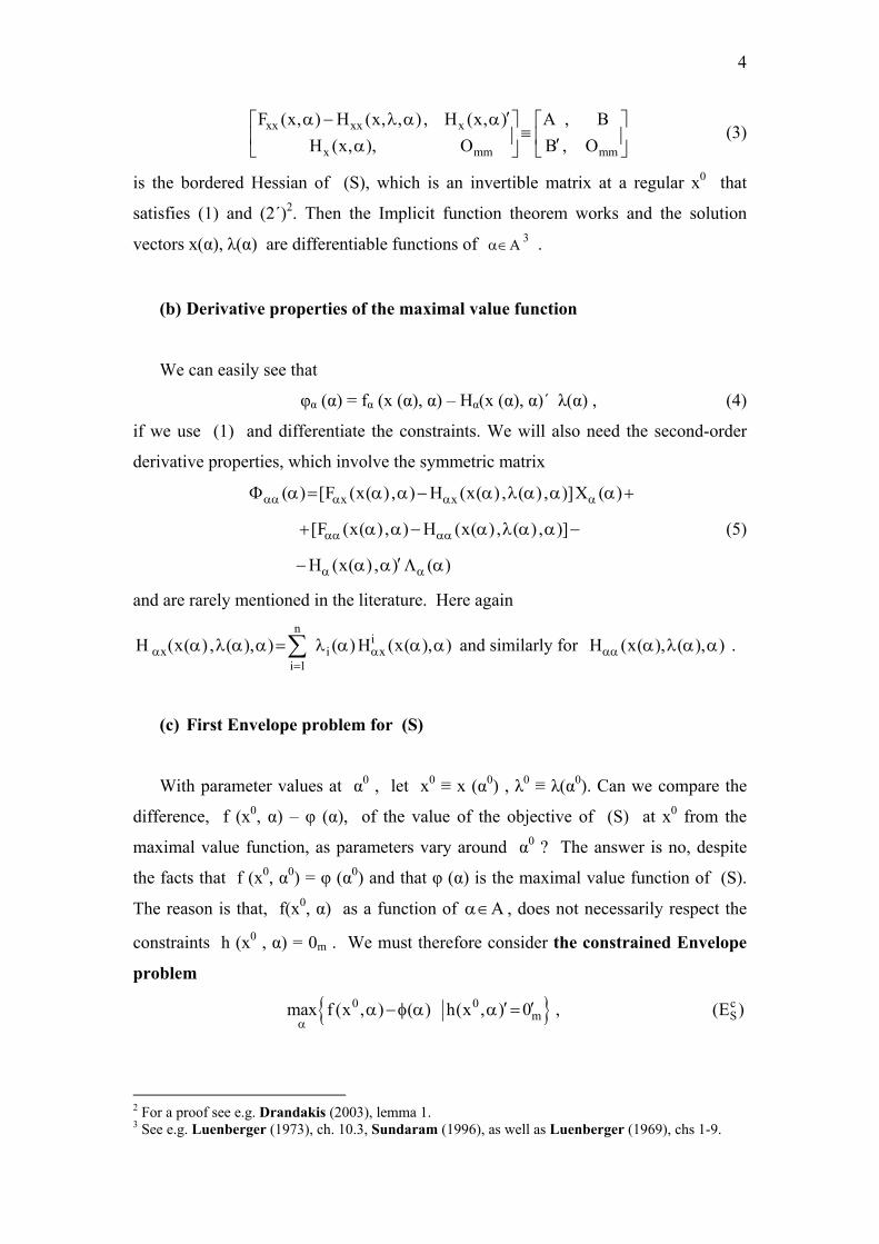
κ΄ - κ = m+ , while

xr(H (x, )) m′α = x(R )

13

also holds. The solution of (H) , x( , )α γ and ˆ ˆ( , ) ( ( , ) , ( , ))+′λ α γ = λ α γ λ α γ ,

satisfies (10) and (11) above appropriately modified, while ( , ) f (x( , ), )ϕ α γ ≡ α γ α

has first and second-order derivative properties corresponding to those in (12) – (14)

and (15) and, finally, the unconstrained Envelope problem 0 0max{f (x , ) ( , h(x , ))}

αα −ϕ α α H(E )

leads to f-o-c and s-o-c corresponding to those in (19) and (20΄) above.

Again ( , ) ( , )ϕ α γ >ϕ α γ , in general, but if we assume that

0 0 0 0 0 0x( , ) x( , ) at ( , )α γ = α γ α γ , then 0 0 0 0 0 0m

ˆ ˆ( , ) ( , ) , ( , ) 0 ++λ α γ = λ α γ λ α γ =

and 0 0 0 0( , ) ( , )ϕ α γ = ϕ α γ .

We can then proceed and consider the second Envelope problem for (H) and

(H)

0 0max{ ( , h(x , ) ( , h(x , )}α

ϕ α α −ϕ α α , HH(E )

which attains a local maximum of zero at 0 0( , )α γ with

00 0 0 0 0

rf o c { H H 0 }′α γ α α γα

′− − ϕ + ϕ −ϕ − ϕ = (27)

and 0 0 0 0 0 0 0 0 0

0 0 0 0 0 0 0 0 0

matrix {[ H ] [H H H H ]

s o c [ H ] [H H H H ]

is negative semi definite (or definite)

′ ′αα αγ α αα α γα α γγ α

′αα αγ α αα α γα α γγ α

⎧ ⎫Φ +Φ + + Φ + Φ −⎪ ⎪⎪ ⎪′− − − Φ +Φ − + Φ + Φ⎨ ⎬⎪ ⎪⎪ ⎪−⎩ ⎭

(28)

At (α0, γ0, γ+0), however, 0 0 0 0H H′ ′α γ α γϕ = ϕ and so we get the far simpler conditions

0 0 0 0 0 0rf o c { ( , h(x , )) ( , h(x , )) 0 }α α− − ϕ α α −ϕ α α = (27΄)

and the curvature conditions for (H) and (H)

0 0 0 0 0x x

0 0 0

matrix [F H ]{X X H ]

s o c [X X H ]}

is negative semi definite (or definite)

α α α γ α

α γ α

⎧ ⎫− + −⎪ ⎪⎪ ⎪− − − +⎨ ⎬⎪ ⎪⎪ ⎪−⎩ ⎭

, (28΄)

14

after using the second-order derivative properties of 0 0 0 0, , andαα αγ αα αγΦ Φ Φ Φ

and cancelling out equal terms with opposite signs.

4. Basic Features of the Primal and Dual Methods for Sensitivity Αnalysis and

Le Chatelier Principle

Having completed the dual method for sensitivity analysis and Le Chatelier

Principle, it is advisable to compare its main features to those of the Primal method.

The primal method can be based on a theorem of Caratheodory (1935, ch. 11 on

ordinary maxima and minima) on the properties of the Inverse of the Bordered

Hessian matrix. Without computing the Inverse mn

A , BU , Vof

B , OV , W⎡ ⎤⎡ ⎤⎢ ⎥⎢ ⎥ ′′⎣ ⎦ ⎣ ⎦

, it can be

easily shown that the n x n U matrix is negative semidefinite with r(U) = n – m, the

m x m matrix W = -V΄ ΑV is positive (semi)definite if A itself happens to be

negative (semi)definite, while r((V) = m and V is a pseudoinverse of B΄ 11. These

results are due to the maximization hypothesis, before we consider parameters

explicitly and the sensitivity of optimal solution to their variations.

The Primal method starts by differentiating the f-o-c of a behavioral system like

(S) or (H) in their respective parameters and solving for the unknown rates of change

of the choice variables.

Thus in (S) we see from (1) that12

x x

mm

[F (x( ), ) H (x( ) , ( ), )]X ( )A , B

H (x( ), )( )B , O

α αα

αα

− α α − α λ α α⎡ ⎤α ⎢ ⎥⎡ ⎤⎡ ⎤

= ⎢ ⎥− α α⎢ ⎥⎢ ⎥′ −Λ α⎣ ⎦ ⎣ ⎦ ⎢ ⎥⎣ ⎦

, (29)

or

11 See Drandakis (2003). When m = n, then U = Onn , W = -B-1 A B-1΄ and V is the inverse of B΄. 12 (29) is called the fundamental matrix equation for comparative static analysis and was introduced by Barten in 1966. For an early application to consumer theory, see Barten, Kloek and Lampars (1969).

15

x x

x x

x x

X ( ) [F HU, V( ) HV , W

U[F H ] VH

V [F H ] WH

α α α

α α

α α α

α α α

α − −⎡ ⎤ ⎡ ⎤⎡ ⎤= =⎢ ⎥ ⎢ ⎥⎢ ⎥′−Λ α −⎣ ⎦⎣ ⎦ ⎣ ⎦

− − −⎡ ⎤⎢ ⎥

= ′⎢ ⎥− −⎢ ⎥⎣ ⎦

(30)

and so we get the curvature conditions

x x x x x x

x x x x x x

m

The x matrix

[F H ]X ( ) [F H ]U[F H ]

[F H ]V H [F H ]U[F H ]

is negative senidefinite (or definite)

on { R H 0 (and 0 )}

α α α α α α α

α α α α α α α

κα κ

⎧ ⎫κ κ⎪ ⎪⎪ ⎪− − α = − − −⎪ ⎪⎪ ⎪− − = − −⎨ ⎬⎪ ⎪⎪ ⎪⎪ ⎪⎪ ⎪ζ∈ ζ = ζ ≠⎩ ⎭

(31)

Clearly (31), as well as (7) above, cannot be used directly for comparative static

analysis since they specify curvature conditions which are subject to constraints. It is

evident, therefore, that a matrix representation of the curvature conditions in the

tangent subspace is needed, irrespective of whether the dual or the primal method

is used. Again with f (x, α) and h (x, α) written as f (x, α, γ) and h (x, α, γ), as we did

above in §2, it can be easily seen that (31) is transformed into the curvature

conditions for (S).

1 1x x x x

1 1x x x x x x x x

The r x r matrix

{ [F H ] H H [F H ]}[X X H H ]

{[F H H H [F H ]}U{F H [F H ] H H ]

is negative semidefinite (or definite)

− −α α α γ γ γ α γ γ α

− −α α α γ γ γ α α γ γ γ α

⎧ ⎫⎪ ⎪⎪ ⎪′′− − + − − =⎪ ⎪⎨ ⎬⎪ ⎪′′= − − − − − − ⋅⎪ ⎪⎪ ⎪⎩ ⎭

. (32)

Similarly in (H) we see from (10) above that

x x m

mm

x x

x x

X , X [F H ], OU, V, H , IV , W

U[F H ] VH , V,

V [F H ] WH , W

α γ α α

α γ α

α α α

α α α

− −⎡ ⎤ ⎡ ⎤⎡ ⎤= =⎢ ⎥ ⎢ ⎥⎢ ⎥−Λ −Λ ′ −⎣ ⎦ ⎣ ⎦⎣ ⎦

− − −⎡ ⎤= ⎢ ⎥′− − −⎣ ⎦

(33)

or, rearranging terms, that

16

x x

x x

X X H U[F H ]H V [F H ]

α γ α α α

α γ α α α

+ − −⎡ ⎤ ⎡ ⎤=⎢ ⎥ ⎢ ⎥−Λ +Λ ′− −⎣ ⎦⎣ ⎦

. (34)

Thus the curvature conditions for (H) are given by

x x

x x x x

[F H ][X X H ]

[F H ]U[F H ]

is negative semidefinite (or definite)

α α α γ α

α α α α

− − + =⎧ ⎫⎪ ⎪⎪ ⎪= − −⎨ ⎬⎪ ⎪⎪ ⎪⎩ ⎭

(35)

exactly as in (18) or (20΄) above.

When, finally, new constraints are added to either (S) or (H), which happen to be

just binding at some x, the comparable submatrices on the main diagonal of the

Inverse of the Bordered Hessian, before and after the introduction of new constraints,

have a structural property that is at the care of Le Chatelier Principle. As shown in

Drandakis (2003) the same curvature conditions, as in (26) for (S) and (28΄) for (H),

are produced.

In conclusion, both methods of sensitivity analysis are quite elegant in matrix

theoretic terms. The primal method appears to be easier and has the advantage that it

stresses some structural properties of the optimization hypothesis that are independent

of the number of parameters and of the way that they appear in the problem. On the

other hand, however, the dual method, utilizes the s-o-c of constrained or

unconstrained Envelope problems and determines the appropriate curvature

conditions in the tangent subspace that are needed for sensitivity analysis and Le

Chatelier Principle. In addition, the Envelope theorem has further important uses,

some of which will be touched on in the following section.

5. An Economic application: The effects of quantity rationing in the Theory of

Consumer Choice

The dual method via the Envelope theorem has been applied to the theory of

consumer choice in Drandakis (2007). A typical consumer is assumed to maximize

17

his utility function n zf (x) , x X R , f C++∈ ⊂ ∈ , subject to an income constraint

w΄x = y, where w > 0n is the price vector and y > 0 is income devoted to

consumption. Under quantity rationing of some goods, f(x) is written as r m mf (x, z), x X R , z Z R++ ++∈ ⊂ ∈ ⊂ and m n+ = , while to w΄x + r΄z = y are

added m new constraints z z= .

We have then for the “first-best” problem

xv(w, y) max{f (x) w x y}′≡ = (Uf)

while the “second-best” optimization problem is given by

x

x,z

v(w, y r z) max{f (x, z) w x y r z} ,or

v(w, r, y, z) max{f (x, z) w x r z y , z z} .

′ ′ ′− ≡ = −

′ ′≡ + = = (Us)

The solution of (Uf) and (Us) is x (w, y) > 0m , λ (w, y) > 0 and

x(w, y r z) 0 , (w, y r z) 0 , or′ ′− > λ − > mx(w, r, y, z) 0 , z(w, r, y, z) z 0> = > ,

>=<

m(w, r, y, z) 0 , (w, r, y, z) 0λ > μ , respectively13, 14 .

The first Envelope problems in both (Uf) and (Us) lead to curvature conditions

w y

n

The n x n matrix[X (w, y) x (w, y) x(w, y) ]

is negative semi definite (or definitefor 0 and tw , t 0)

⎧ ⎫⎪ ⎪′+⎪ ⎪⎨ ⎬

−⎪ ⎪⎪ ⎪η ≠ η ≠ >⎩ ⎭

and

w y

The x matrix[X (w, r, y, z) x (w, r, y, z) x(w, r, y, z) ]

is negative semi definite (or definitefor 0 and tw , t 0)

⎧ ⎫⎪ ⎪′+⎪ ⎪⎨ ⎬

−⎪ ⎪⎪ ⎪η ≠ η ≠ >⎩ ⎭

respectively, no matter whether they are constrained problems and need a matrix

representation in the tangent subspace or are unconstrained.

13 Due to the equality rationing constraints, their respective multipliers, j (w, r, y, z) , j 1, ..., mμ =

may be positive, zero or negative depending on whether j jz z (w,r, y)<=>

. 14 Clearly (Uf) and (Us) are special cases of (H) and (H) with linear constraints. There is, however, a new feature in (Us) : some choice variables become parameters.

18

When however, we examine the interrelations between (Uf) and (Us), it is

quickly realized that the Envelope theorem has a far greater scope than our analysis in

§ 3 may have led us to expect.

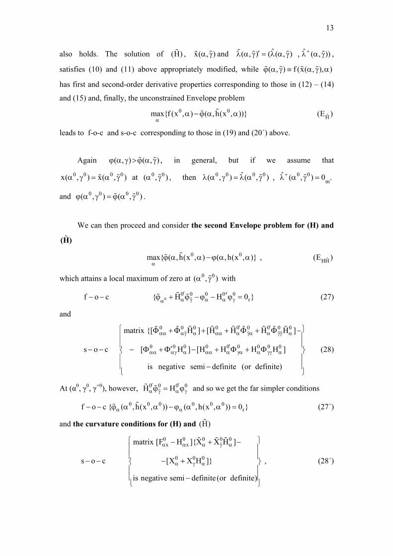
Indeed, four Le Chatelier effects can be distinguished between (Uf) and (Us). As

the following diagram illustrates15, in panel (i) our consumer has solved (Uf) at point

A. When threatened with quantity rationing, z , he wishes first to consider the damage

inflicted under the best possible circumstances. He thus attains an Envelope tangency

at A by choosing z z(w, r, y)≡ and so he gets x(w, r, y, z) x(w, r, y)≡ ,

(w, r, y, z) (w, r, y)λ ≡ λ and m(w, r, y, z) 0μ ≡ . Thus when w and y vary, while z

respond appropriately, we obtain the curvature conditions16

s s s f f fw y w y

The x matrix

[X x x ] [X x x ]

is negative semi definite, withat least negative main diagonal

elements

⎧ ⎫⎪ ⎪

′ ′+ − +⎪ ⎪⎪ ⎪−⎨ ⎬⎪ ⎪⎪ ⎪⎪ ⎪⎩ ⎭

(36)

This is, of course, Samuelson’s (1947) original Le Chatelier Principle, as has

been applied to the theory of consumer choice by Tobin and Houthakker (1950) and

Pollak (1969). We also note that no Envelope problem is needed. Similarly, in

panel (ii), where (Us) has been solved, at point A, our consumer may wish to

ascertain how much better off he would have been if he were forced there while

solving (Uf), under appropriate “shadow” prices of rationed goods r and income,

y y (r r) z′= + − . In fact this can be done if he chooses

zr (1/ (w, r, y, z) f (x (w, r, y, z), z)≡ λ ≡ mr (1/ (w, r, y, z)) (w, r, y, z) 0+ λ μ > . Then

he would attain an Envelope tangency at A with x(w, r, y) x(w, r, y, z)≡ ,

z(w, r, y) z≡ and (w, r, y) (w, r, y, z)λ ≡ λ . Thus when w and y vary, while

r and y respond appropriately, we obtain the curvature conditions

15 The diagram serves its purpose, despite its simplicity, with m 1 and n 2= = = . 16 An ~ superscript indicates x(w, r, y, z) and its rates of change in w and y.

19

s s s f f fw y w y

The x matrix

[X x x ] [X x x ]

is negative semi definite, withat least negative main diagonal

elements

⎧ ⎫⎪ ⎪

′ ′+ − +⎪ ⎪⎪ ⎪−⎨ ⎬⎪ ⎪⎪ ⎪⎪ ⎪⎩ ⎭

(37)

But that is not all! In panel (iii) our consumer has solved (Uf) at point A, but is

forced to consume z z(w, r, y)≠ in the second-best solution at point B. He can then

solve the Envelope problem

r̂ˆ ˆmax{v(w, r, y, z) v(w, r, y (r r) z)}′− + − r̂(E )

and determine the shadow price vector, r , implicitly from z z(w, r, y (r r) z)′≡ + −

and y y (r r) z′≡ + − 17. Thus the consumer attains an Envelope tangency at the

second - best (Us) at point B, with x (w, r, y, z) x (w, r, y (r r) z)′≡ + − ,

z z(w, r, y (r r) z)′≡ + − and (w, r, y, z) (w, r, y (r r) z)′λ ≡ λ + − . Thus as w and y

vary, while r and y respond, we obtain the same curvature conditions as in (37),

despite the completely different mechanism that generates them.

Finally, in panel (iv), a consumer who has solved (Us) at point A may still be

interested in solving the Envelope problem

zmax{v(w, r, y, z) v(w, r, y)}− z(E )

and derive z implicitly from z mv (w, r, y, z) (w, r, y, z) 0≡ μ ≡ 18. If m(w, r, y, z) 0μ ≠ ,

then clearly z z≠ and point B is different from A. With

x(w, r, y) x(w, r, y, z) , z(w, r, y) z≡ ≡ and (w, r, y) (w, r, y, z)λ ≡ λ , when w and y

vary, while z responds, we attain an Envelope tangency at the first-best maximum, at

B, with curvature conditions which appear as in (36) above.

17 As shown in Drandakis (2007), a local maximum of zero is attained in r(E ) by the above choice of

r and y . Indeed r̂

ˆ ˆv(w, r, y, z) min{v(w, r, y, (r r) z)} v(w, r, y (r r) z)′ ′= + − = + − .

18 Again a local maximum of zero is attained in (E )z by the choice of z . Here

zv(w, r, y, ) max{v(w, r, y, z)} v(w, r, y, z)= = .

20

f s s f(U ) at A (U ) at A (U ) at A (U ) at A→ →

panel (i) panel (ii)

f s s f

r z(U ) at A (E ) (U ) at B (U ) at A (E ) (U ) at B+ → + → panel (iii) panel (iv)

Figure

Panels (i), (ii), (iii) and (iv). Initial utility maxima at A and Envelope tangencies at

A or B.

uf

A

z

z

x

zf

y / r

0 f s fx x x y / w y / w=

fz z= us

B

z

uf

A

y/r

fz z=

z

0 s fx x y / w= x

0 f sx x y / w y / w=

z

y/r

y / r

fz z=A

us

x

0 f s sx x x y / w=

z

y/r

fz z=

z A

us

B

x

21

6. Concluding Remarks

The dual method for sensitivity analysis and Le Chatelier Principle, in general

static optimization problems, has been presented here. The method is based on the

curvature conditions derived from appropriate Envelope problems, in which former

parameters become the choice variables and vice versa.

These envelope problems may be either constrained or unconstrained – depending

on the parametric structure of the original problem – and may lead to second-order

conditions that are subject to constraints. In that event, a further effort is needed for

deriving their representation in tangent subspaces and thus producing the suitable

curvature conditions. An important role in this process is played by second-order

derivative properties of the maximum value functions of the optimization problems.

Despite the early appearance of the two basic papers of Silberberg (1974) and

Hatta (1986), the development of a unified dual method via the Envelope theorem

has been undoubtedly delayed by the almost exclusive attention given in the literature

to first-order envelope tangencies and the rate mention of the fact that the desired

curvature conditions are derived from second-order envelope conditions. Indeed, it is

quite clear that the “primal-dual method” of Silberberg, i.e., 0 0 0

mmin{d( , x )} min{ ( ) f (x , ) h(x , ) 0 }α α

′ ′α ≡ ϕ α − α α = (PDS)

is exactly our first envelope problem for (S), while the “gair function method” of

Hatta, i.e., 0 0 0min{g( , x )} min{ ( , h(x , )) f (x , )}

α αα ≡ ϕ α α − α (GH)

is the unconstrained version of our first envelope theorem for (H). Yet, Silberberg

(1974), pg. 162, considers the f-o-c of cS(E ) as tantamount to “the famous envelope

theorem developed by Samuelson”, while Hatta (1980), pg. 900, calls his

theorem 4 - about rf (x( , ), ) {X ( , ) X ( , ) H (x ( , ), )} 0α α γ α′ ′α γ α α γ + α γ α γ α = - as

“the first envelope theorem” and his theorem 5 on

( , ) H (x( , ), ) ( , ) f (x( , ), )α α γ α′ϕ α γ + α γ α ϕ α γ = α γ α as “the second envelope theorem”.

22

In a more recent contribution, Caputo (1996) examines the Hatta model and, in

his main theorem, he proves that the unconstrained gain optimization problem (GH)

and the constrained primal – dual optimization problem for (H), i.e., 0 0 0

, ,min{d( , , x )} min{ ( , ) f (x , ) h(x , ) }α γ α γ

′ ′α γ ≡ ϕ α γ − α α = γ (PDH)

lead to the same curvature conditions. Indeed, Caputo has proved the constrained

version of the first envelope problem for (H), cH(E ) of section 2(f). Caputo does not

attempt to derive the appropriate curvature conditions for (S), although he notes that

the primal - dual method can be applied to the more general Silberberg model19.

We may wonder, therefore, despite the claim of Hatta (1987), pg. 157, that

several authors “have simplified the proof methods of the Le Chatelier Principle by

regarding the principle as an envelope result, following Mc Kenzie’s (1957) proof of

the negative semidefiniteness of the substitution matrix”, whether the impact of the

Envelope theorem for sensitivity analysis and Le Chatelier Principle was fully

appreciated in the relevant literature and whether it were exploited with commendable

rapidity.

19 Caputo, too, notes in pg. 244 that “the first-order necessary conditions [gα (α0, x0) = 0r ] yield a one line proof of the envelope theorem for [(H)]”.

23

REFERENCES

Barten A., T. Kloek and F. Lempars (1969), “A note on a class of utility and production functions yielding everywhere differentiable dement functions”, Review of Economic Studies, 109-111.

Caputo M., (1996), “The relationship between two dual methods of comparative

statics”, Journal of Economic Theory, 243-250. Caratheodory C., (1935), Calculus of Variations and Partial Differentiable Equations

of the First Order, in German. English translation, 1967, Holden Day. Drandakis E., (2003), “Caratheodory’s theorem on constrained optimization and

comparative statics”, Discussion Paper, Athens University of Economics and Business.

___________ (2007), “The envelope theorem at work: utility (output) maximization

under straight rationing”, Discussion Paper, Athens University of Economics and Business.

Hatta T., (1980), “The structure of the correspondence principle at an extremum

point”, Review of Economic Studies, 987-997. ________ (1987), “Le Chatelier Principle”, in New Palgrave: A Dictionary of

Economics, 3, pp. 155-157, Macmillan. Luenberger D., (1969), Optimization by Vector Space Methods, Wiley. ___________ (1973), Introduction to Linear and Nonlinear Programming, Addison-

Wesley. McKenzie L., (1957), “Demand Theory without a utility index”, Review of Economic

Studies, 185-189. Pollak R., (1969), “Conditional demand functions and consumption theory” Quarterly

Journal of Economics, 60-78. Samuelson P., (1947), Foundations of Economic Analysis, Harvard University Press. Silberberg E., (1974), “A revision of comparative static methodology in economics”,

Journal of Economic Theory, 159-172. Sunbaram R., (1996), A First Course in Optimization Theory, Cambridge University

Press. Tobin J. and H. Houthakker, (1951), “The effects of rationing on demand elasticities”,

Review of Economic Studies, 140-153.

24

Appendix A:

In § 2(c), the product matrix 10 0 0 0 0

rrZ C Z [I , H H ]− ′′

α γ′ = −

1

0 0 0 0 0 0 0 0 0 0rrx x x x

0 00 0 0 0 0 0 0 0 0 0x x x x

I[F H ]X H , [F H ]X H

H H[F H ]X H , [F H ]X H−

′ ′α α α α α α α γ α γ

′ ′γ αγ γ α γ α γ γ γ γ γ

⎡ ⎤ ⎡ ⎤− − + Λ − − + Λ=⎢ ⎥ ⎢ ⎥

−− − + Λ − − + Λ⎢ ⎥ ⎢ ⎥⎣ ⎦⎣ ⎦

1 10 0 0 0 0 0 0 0 0 0 0 0 0 0x x x x x x x x{[ [F H ] H H [F H ]]X ,[ [F H ] H H [F H ]]X ]}

− −′ ′′ ′α α α γ γ γ α α α α γ γ γ γ= − − + − − − + −

1 1

1

rr 0 0 0 0 0 0 0 0 0 0x x x x0 0

I[ [F H ] H H [F H ]][X X H H ] ,

H H− −

−′′

α α α γ γ γ α γ γ αγ α

⎡ ⎤= − − + − −⎢ ⎥

−⎢ ⎥⎣ ⎦

exactly as appears in (8).

Appendix B:

In § 2 (f), we may offer an alternative proof of the unconstrained Envelope

problem (EH), if we follow Hatta (1980) and modify (H) itself in an appropriate

way. Indeed let us define, for any x X , x( ; x) x( , h (x, ))∈ α ≡ α α and

( ; x) ( , h (x , ))λ α ≡ λ α α and note that, although x( ; x) xα ≠ in general, we get

X ( ; x) X ( ,h (x , )) X ( ,h (x , )) H (x, )α α γ αα = α α + α α α and

( ; x) ( , h (x, )) ( , h (x, )) H (x, )α α γ αΛ α = Λ α α +Λ α α α connecting the derivatives

of x( ; x) and ( ; x)α λ α with those of the solution of (H), when constraint levels

also vary so as to keep h(x, ) h(x ; )α = α . We see therefore that we can get an

unconstrained Envelope problem, if we consider the compensated version of (H), i.e.,

x( ; x) max{f (x, ) h(x, ) h(x , ) }′ ′ϕ α ≡ α α = α , (Hcomp)

whose solution x( ; x) and ( ; x)α λ α satisfy (10) and (11) in the text, appropriately

modified.

We also have ( ; x) f (x( ; x), ) ( , h(x, ))ϕ α ≡ α α ≡ ϕ α α with

( ; x) f (x( ; x), ) [H (x( ; x), ) H (x, )] ( ; x)α α α α ′ϕ α = α α − α α − α λ α

25

and c c c c c c c cx x( ; x) [F H ]X [F H H (x, , )] [H H (x, )]αα α α α αα αα αα α α α′Φ α = − + − + λ α − − α Λ .

Here superscript c indicates that the respective matrices are evaluated at x( ; x)α and

( ; x)λ α .

Of course, we are not interested in any odd x but in studying the impact of

variations in α and γ evaluated at a solution of (H). Thus for any (α0, γ0) let

x0 = x (α0, γ0) and λ0 = λ (α0, γ0) with x (α0 ; x0) = x0 and λ (α0 ; x0) = λ0. We can

then consider the unconstrained Envelope problem 0 0max{f (x , ) ( ; x )}

αα −ϕ α , co mp

H(E )

with 0 0

rf o c {f (x , ) ( ; x ) 0 }α α− − α −ϕ α =

and 0 0[F (x , ) ( ; x )] is as o c

negative semidefinite (or definite) matrixαα αα⎧ ⎫α −Φ α⎪ ⎪− − ⎨ ⎬

⎪ ⎪⎩ ⎭

satisfied at α0 with x (α0 ; x0) = x0. We also see that φα (α0 ; x0) = fα (x0 ;α0) and 0 0 0c 0c 0c 0c

x ex( ; x ) [F H ]X Fαα α α ααΦ α = − + and thus we get the curvature conditions of (20)

in the text.

Appendix C:

In § 3, the s-o-c of SS(E ) involve the κ x κ matrix

00 0 0 0 0 0x x

m m

[F H ][X X ] H [ ]O + +

αα α α α α α

⎡ ⎤Λ′− − − Λ − ⎢ ⎥⎢ ⎥⎣ ⎦

.

When α becomes ( , )α γ , the above matrix is written as

0 0 0 0 0x x 0 0 0 0 0 00 0 0x x m m m m

F H H[X X ,X X ] [ , ] .

O OF H H

(r m ) x n n x (r m ) (r m ) x m m x (r m )

+ + + +

α α α α γα α γ γ α γ

γ γ γ

⎡ ⎤′⎡ ⎤ ⎡ ⎤ ⎡ ⎤− Λ Λ⎢ ⎥− − − Λ − Λ −⎢ ⎥ ⎢ ⎥ ⎢ ⎥⎢ ⎥′−⎢ ⎥ ⎢ ⎥ ⎢ ⎥⎣ ⎦ ⎣ ⎦⎣ ⎦ ⎣ ⎦

′ ′ ′ ′ ′ ′ ′ ′ ′ ′+ + + +

26

When this matrix is multiplied on the left by 0 0 0 1r rZ [I , H H ]−′ ′ α γ

′ ′ ′= − it gives us the

r΄ x κ matrix 1

1

1

0 0 0 0 0 0 0 0 0x x x x

0 00 0 0 0 0 0

m m m m

0 0 0 0 0 0 0 0 0x x x x

{F H H H [F H ]}[X X , X X ]

[H H H H ][ , ]O O

{F H H H [F H ]}[X X , X X ] ,

−

−

+ + + +

−

′α α α γ γ γ α α γ γ

′ α γα α γ γ α γ

′α α α γ γ γ α α γ γ

′− − − − − −

⎡ ⎤ ⎡ ⎤Λ Λ′ ′ ′− − Λ − Λ − =⎢ ⎥ ⎢ ⎥⎢ ⎥ ⎢ ⎥⎣ ⎦ ⎣ ⎦

′= − − − − −

which, when multiplied on the right by Z0 , gives us (26).

Again it should be noted how helpful matrix notation is in carrying out such

complex operations.