4. Duality 21 4.1 Duality of LPs and the duality theorem ...page.math.tu-berlin.de/~moehring/adm2/Chapter/chap4.pdf · 4.3 The shortest path problem and its dual ... 22-8 dual primal

4. Duality

21

..................................................................................................................................... 224.1 Duality of LPs and the duality theorem........................................................................................................................................................ 234.2 Complementary slackness

..................................................................................................................................... 244.3 The shortest path problem and its dual.......................................................................................................................................................................... 254.4 Farkas' Lemma

.................................................................................................................................................. 264.5 Dual information in the tableau....................................................................................................................................................... 274.6 The dual Simplex algorithm

4. Duality4.1 Duality of LPs and the duality theorem

22-1

The dual of an LP in general form

Derivation of the dual

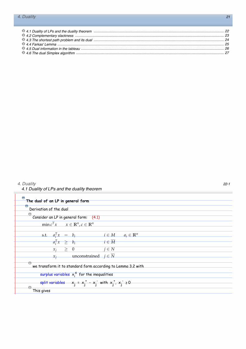
Consider an LP in general form: (4.1)

min cTx x ∈ Rn, c ∈ Rn

s.t. aTi x = bi i ∈ M ai ∈ Rn

aTi x ≥ bi i ∈ M

xj ≥ 0 j ∈ Nxj unconstrained j ∈ N

we transform it to standard form according to Lemma 3.2 with

surplus variables xis for the inequalities

split variables xj = xj+ - xj

- with xj+, xj

- ! 0

This gives


22-2

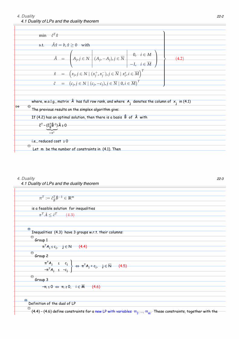
min cT x

s.t. Ax = b, x ≥ 0 with

A =

Aj, j ∈ N

��(Aj,−Aj), j ∈ N

��

0, i ∈ M

−I, i ∈ M

x =�

xj, j ∈ N | (x+j , x−j ), j ∈ N | xsi , i ∈ M

�T

c =�cj, j ∈ N | (cj,−cj), j ∈ N | 0, i ∈ M

�T

(4.2)

where, w.o.l.g., matrix !! has full row rank, and where Aj denotes the column of xj in (4.1)

The previous results on the simplex algorithm give:

If (4.2) has an optimal solution, then there is a basis !! of !! with

!!" ! "!!"!#!#!#$

� �� %&$"

!% " '

i.e., reduced cost ! 0

Let m be the number of constraints in (4.1). Then


22-3

πT := cTB B−1 ∈ Rm

is a feasible solution for inequalities

πT A ≤ cT (4.3)

Inequalities (4.3) have 3 groups w.r.t. their columns:

Group 1!"#$ ! %$& $ ∈ ' !"("#

Group 2

!"#$ ! %$

"!"#$ ! "%$

⇔ !"#$ ! %$& $ ∈ ' "#($%

Group 3

!!" " ! ⇔ !" # !# " ∈ $ "#%$%

Definition of the dual of LP

(4.4) - (4.6) define constraints for a new LP with variables π1, ..., πm. These constraints, together with the

objective function max πTb constitute the dual LP of (4.1). The initial problem (4.1) is called the primal LP.


22-4

objective function max πTb constitute the dual LP of (4.1). The initial problem (4.1) is called the primal LP.

Transformation rules primal -> dual (follow from (4.4) - (4.6))

primal dual

min cTx max πT b

aTi x = bi i ∈ M πi unconstrained

aTi x ≥ bi i ∈ M πi ≥ 0

xj ≥ 0 j ∈ N πTAj ≤ cj

xj unconstrained j ∈ N πTAj = cj

Observe: The dual LP is obtained from the optimality criterion of the primal. The variables π1, ..., πm

correspond to multipliers of the rows of !! that fulfill the primal optimality criterion.

4.1 Theorem (dual dual = primal)

The dual of the dual is the primal.

We therefore speak of primal-dual pairs of LPs

Proof

Write the dual in primal form:


22-5

Write the dual in primal form:

min πT (−b) such that

(−ATj )π ≥ −ci j ∈ N

(−ATj )π = −ci j ∈ N

πi ≥ 0 j ∈ M

πi unconstrained j ∈ M

The transformation rules yield the following dual LP

max xT (−c) such that

xj ≥ 0 j ∈ N

xj unconstrained j ∈ N

−aTi x ≤ −bi i ∈ M

−aTi x = −bi i ∈ M

which is the primal LP !

The Duality Theorem

4.2 Theorem (Weak and Strong Duality Theorem)

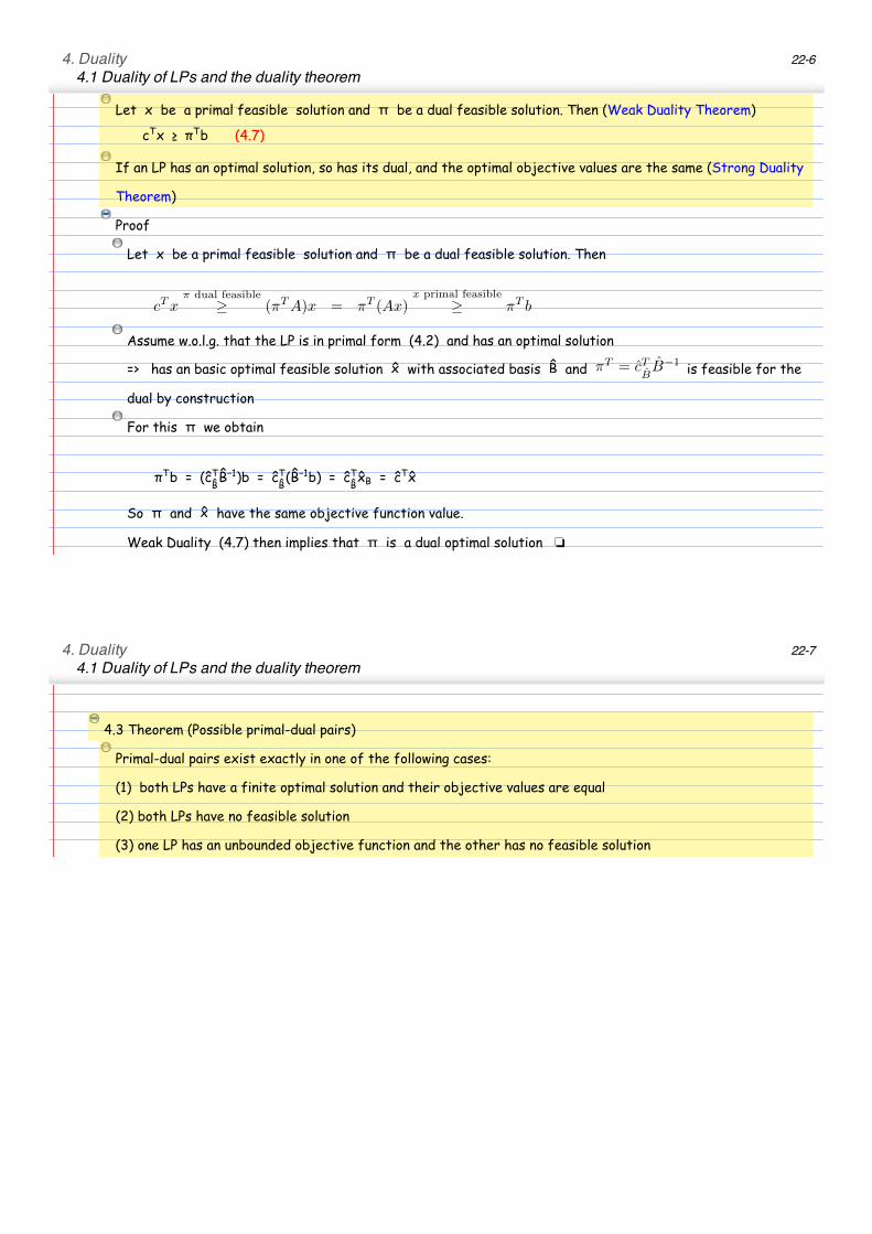
Let x be a primal feasible solution and π be a dual feasible solution. Then (Weak Duality Theorem)


22-6

Let x be a primal feasible solution and π be a dual feasible solution. Then (Weak Duality Theorem)

!"# ! $

"% !"&#$

If an LP has an optimal solution, so has its dual, and the optimal objective values are the same (Strong Duality

Theorem)

Proof

Let x be a primal feasible solution and π be a dual feasible solution. Then

cTxπ dual feasible

≥ (πTA)x = πT (Ax)x primal feasible

≥ πT b

Assume w.o.l.g. that the LP is in primal form (4.2) and has an optimal solution

=> has an basic optimal feasible solution !! with associated basis !! and πT = cTBB−1

is feasible for the

dual by construction

For this π we obtain

!"# ! "#$"#%

#%!$%# ! #$"#%"#%!$

#% ! #$"#%#&% ! #$"#&

So π and !! have the same objective function value.

Weak Duality (4.7) then implies that π is a dual optimal solution !


22-7

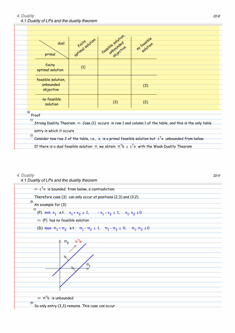
4.3 Theorem (Possible primal-dual pairs)

Primal-dual pairs exist exactly in one of the following cases:

(1) both LPs have a finite optimal solution and their objective values are equal

(2) both LPs have no feasible solution

(3) one LP has an unbounded objective function and the other has no feasible solution


22-8

dual

primal

finiteoptimal solution

finite

optimal s

olutio

n

feasib

le sol

ution,

unboun

ded

objec

tive no

feasib

le

soluti

on

feasible solution,unboundedobjective

no feasiblesolution

(1)

(3)

(2)(3)

Proof

Strong Duality Theorem => Case (1) occurs in row 1 and column 1 of the table, and this is the only table

entry in which it occurs

Consider now row 2 of the table, i.e., x is a primal feasible solution but cTx unbounded from below.

If there is a dual feasible solution π, we obtain πTb " cTx with the Weak Duality Theorem

=> cTx is bounded from below, a contradiction.


22-9

=> cTx is bounded from below, a contradiction.

Therefore case (3) can only occur at positions (2,3) and (3,2)

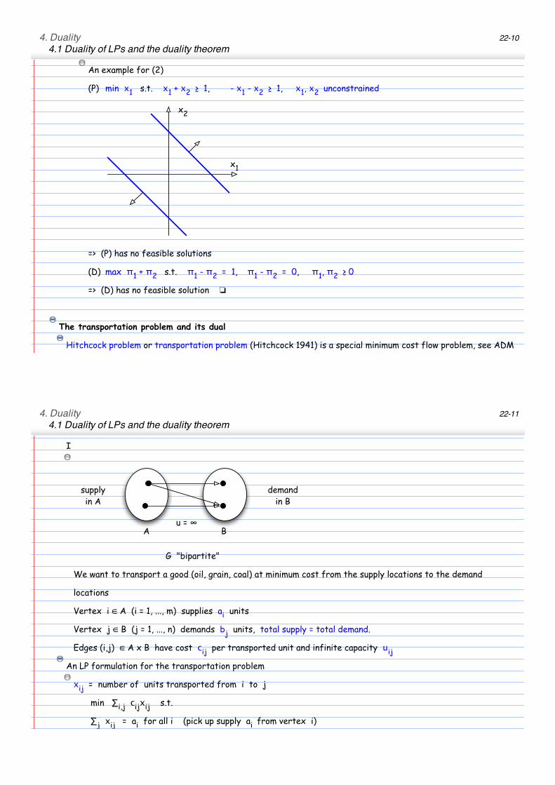
An example for (3)

(P) min x1 s.t. x1 + x2 ! 1, - x1 - x2 ! 1, x1, x2 ! 0

=> (P) has no feasible solution

(D) max π1 + π2 s.t. π1 - π2 " 1, π1 - π2 " 0, π1, π2 ! 0

!1

!2 !

Tb

=> πTb is unbounded

So only entry (3,3) remains. This case can occur

An example for (2)


22-10

An example for (2)

(P) min x1 s.t. x1 + x2 ! 1, - x1 - x2 ! 1, x1, x2 unconstrained

x1

x2

=> (P) has no feasible solutions

(D) max π1 + π2 s.t. π1 - π2 = 1, π1 - π2 = 0, π1, π2 ! 0

=> (D) has no feasible solution !

The transportation problem and its dual

Hitchcock problem or transportation problem (Hitchcock 1941) is a special minimum cost flow problem, see ADM

I


22-11

I

supplyin A

demandin B

A Bu = !

G "bipartite"

We want to transport a good (oil, grain, coal) at minimum cost from the supply locations to the demand

locations

Vertex i ∈ A (i = 1, ..., m) supplies ai units

Vertex j ∈ B (j = 1, ..., n) demands bj units, total supply = total demand.

Edges (i,j) ∈ A x B have cost cij per transported unit and infinite capacity uij

An LP formulation for the transportation problem

xij = number of units transported from i to j

min #i,j cijxij s.t.

#j xij = ai for all i (pick up supply ai from vertex i)

#i xij = bj for all j (deliver demand bj to vertex j )


22-12

#i xij = bj for all j (deliver demand bj to vertex j )

xij ! 0 for all i, j

The associated matrix A of coefficients has the formi =

1,...

,mj

= 1,

...,n

!!! !!" " " " !!# !"! !"" " " " !"# " " " !$! !$" " " " !$#

! ! " " " ! # # " " " # " " " # # " " " #

# # " " " # ! ! " " " ! " " " # # " " " #

$ $ $$ $ $

$ $ $$ $ $

# # " " " # # # " " " # " " " ! ! " " " !

! # " " " # ! # " " " # " " " ! # " " " #

# ! " " " # # ! " " " # " " " # ! " " " #

$ $ $$ $ $

$ $ $$ $ $

# # " " " ! # # " " " ! " " " # # " " " !

The dual of the transportation problem

Introduce dual variables ui, vj for the constraints as follows

ui - #j xij = - ai for all i

vj #i xij = bj for all j

The dual LP reads

max #i - aiui + #j bjvj s.t.


22-13

max #i - aiui + #j bjvj s.t.

- ui + vj " cij for all i, j

ui, vj unconstrained

Interpretation of the dual LP

"Dual" entrepreneur offers to do the transportation for pairs (i,j)

He can buy the supply ai at location i from the primal entrepreneur, transport it to j and sell it there

ui = price to buy a unit of the good at vertex i

vj = returns per unit at vertex j

vj - ui = profit per unit bought in i and sold in j

vj - ui " cij dual entrepreneur must stay below primal transportation cost in order to get the transport (i,j)

from the primal entrepreneur (otherwise primal entrepreneur will do it himself)

Dual entrepreneur wants to maximize his total profit #j bjvj - #i aiui under these conditions

The dual of the diet problem

The primal problem (see example 3.1)

min cTx

s.t. Ax ! r

x ! 0


22-14

x ! 0

The associated dual problem

max πTr

s.t. πTA " cT

πT ! 0

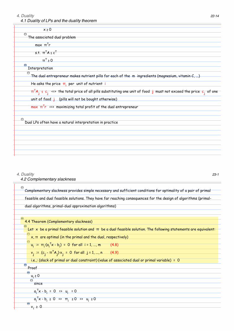
Interpretation

The dual entrepreneur makes nutrient pills for each of the m ingredients (magnesium, vitamin C, ...)

He asks the price πi per unit of nutrient i

πTAj " cj <=> the total price of all pills substituting one unit of food j must not exceed the price cj of one

unit of food j (pills will not be bought otherwise)

max πTr <=> maximizing total profit of the dual entrepreneur

Dual LPs often have a natural interpretation in practice

4. Duality4.2 Complementary slackness

23-1

Complementary slackness provides simple necessary and sufficient conditions for optimality of a pair of primal

feasible and dual feasible solutions. They have far reaching consequences for the design of algorithms (primal-

dual algorithms, primal-dual approximation algorithms)

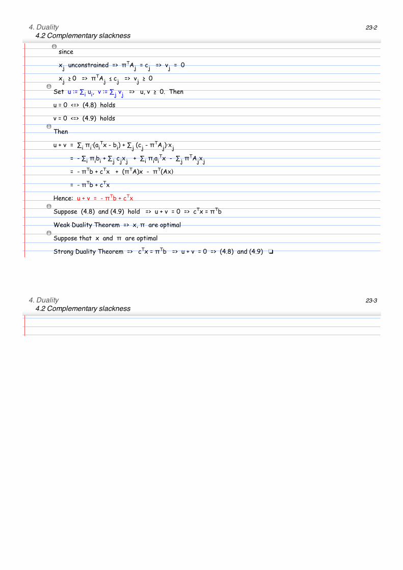
4.4 Theorem (Complementary slackness)

Let x be a primal feasible solution and π be a dual feasible solution. The following statements are equivalent:

x, π are optimal (in the primal and the dual, respectively)

ui := πi·(aiTx - bi) = 0 for all i = 1, ..., m (4.8)

vj := (cj - πTAj)·xj = 0 for all j = 1, ..., n (4.9)

i.e.,: (slack of primal or dual constraint)·(value of associated dual or primal variable) = 0

Proof

ui ! 0

since

aiTx - bi = 0 => ui = 0

aiTx - bi ! 0 => πi ! 0 => ui ! 0

vj ! 0


23-2

since

xj unconstrained => πTAj = cj => vj = 0

xj ! 0 => πTAj " cj => vj ! 0

Set u := #i ui, v := #j vj => u, v ! 0. Then

u = 0 <=> (4.8) holds

v = 0 <=> (4.9) holds

Then

u + v = #i πi·(aiTx - bi) + #j (cj - πTAj)·xj

= - #i πibi + #j cjxj + #i πiaiTx - #j πTAjxj

= - πTb + cTx + (πTA)x - πT(Ax)

= - πTb + cTx

Hence: u + v = - πTb + cTx

Suppose (4.8) and (4.9) hold => u + v = 0 => cTx = πTb

Weak Duality Theorem => x, π are optimal

Suppose that x and π are optimal

Strong Duality Theorem => cTx = πTb => u + v = 0 => (4.8) and (4.9) !


23-3

4. Duality4.3 The shortest path problem and its dual

24-1

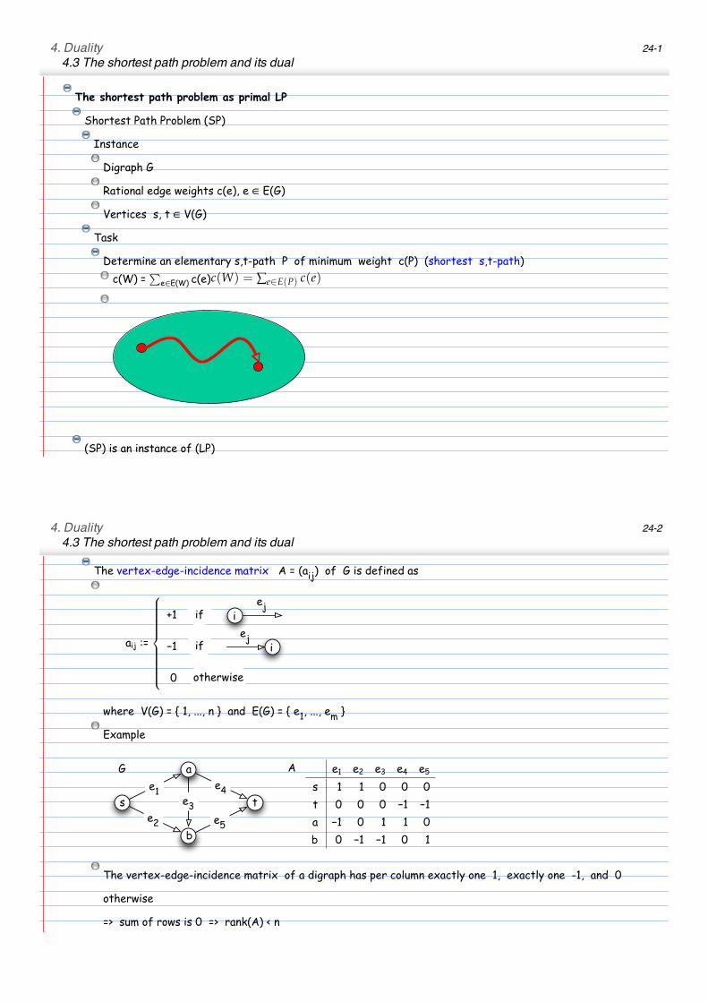
The shortest path problem as primal LP

Shortest Path Problem (SP)

Instance

Digraph G

Rational edge weights c(e), e ∈ E(G)

Vertices s, t ∈ V(G)

Task

Determine an elementary s,t-path P of minimum weight c(P) (shortest s,t-path)!!"" #

�#∈$!"" !!#"c(W) = ∑e∈E(P) c(e)

(SP) is an instance of (LP)


24-2

The vertex-edge-incidence matrix A = (aij) of G is defined as

iej

iej!"# !"

#$ %&''(

!$ %&''(

) (*+(,

if

if

otherwise

where V(G) = { 1, ..., n } and E(G) = { e1, ..., em }

Example

s

a

b

t

e1

e2

e3

e4

e5

G

!! !" !# !$ !%

" ! ! & & &

# & & & !! !!

$ !! & ! ! &

% & !! !! & !

A

The vertex-edge-incidence matrix of a digraph has per column exactly one 1, exactly one -1, and 0

otherwise

=> sum of rows is 0 => rank(A) < n

Later: rank(A) = n-1 if G is connected (in the undirected sense)


24-3

Later: rank(A) = n-1 if G is connected (in the undirected sense)

Let fj be a variable representing the amount of flow on edge ej, and let f := (f1, ..., fm )T

Flow conservation in node i is then expressed as aiTf = 0

v302

4

1

inflow in v = 5 = outflow from v

An s,t-path is a flow of flow value 1 from s to t (all fj = 1 on the path and 0 otherwise)

=> every s,t-path is a solution of the linear system

row srow t

flow conservation

!" ! # "#$ # !

%$

!$

&

'''

&

Af = b with

with v = 1

Of course, this linear system has also solutions that do not correspond to s,t-paths. But we have


24-4

4.6 Lemma

(1) If

min cTf

Af = b

f ! 0

has an optimal solution, then also one with fj ∈ { 0, 1 }. Every such solution corresponds to an s,t-path

(2) The simplex algorithm finds such a solution

Proof:

(1) follows from the algorithm for minimum cost s,t-flows in ADM I

(2) can easily be shown directly, but follows also from the fact that matrix A is totally unimodular and b

is integer. Then all basic feasible solutions of the LP are integer. We will show this more general result in

Chapter 7.2. !

Solving (SP) with the simplex algorithm

We formulate (SP) as (LP)

min cTf


24-5

min cTf

Af = b (A = vertex-edge-incidence matrix )

f ! 0

and solve it with the simplex algorithm.

Since rank(A) < n, we may delete a row

=> delete the row for vertex t, this yields b ! 0

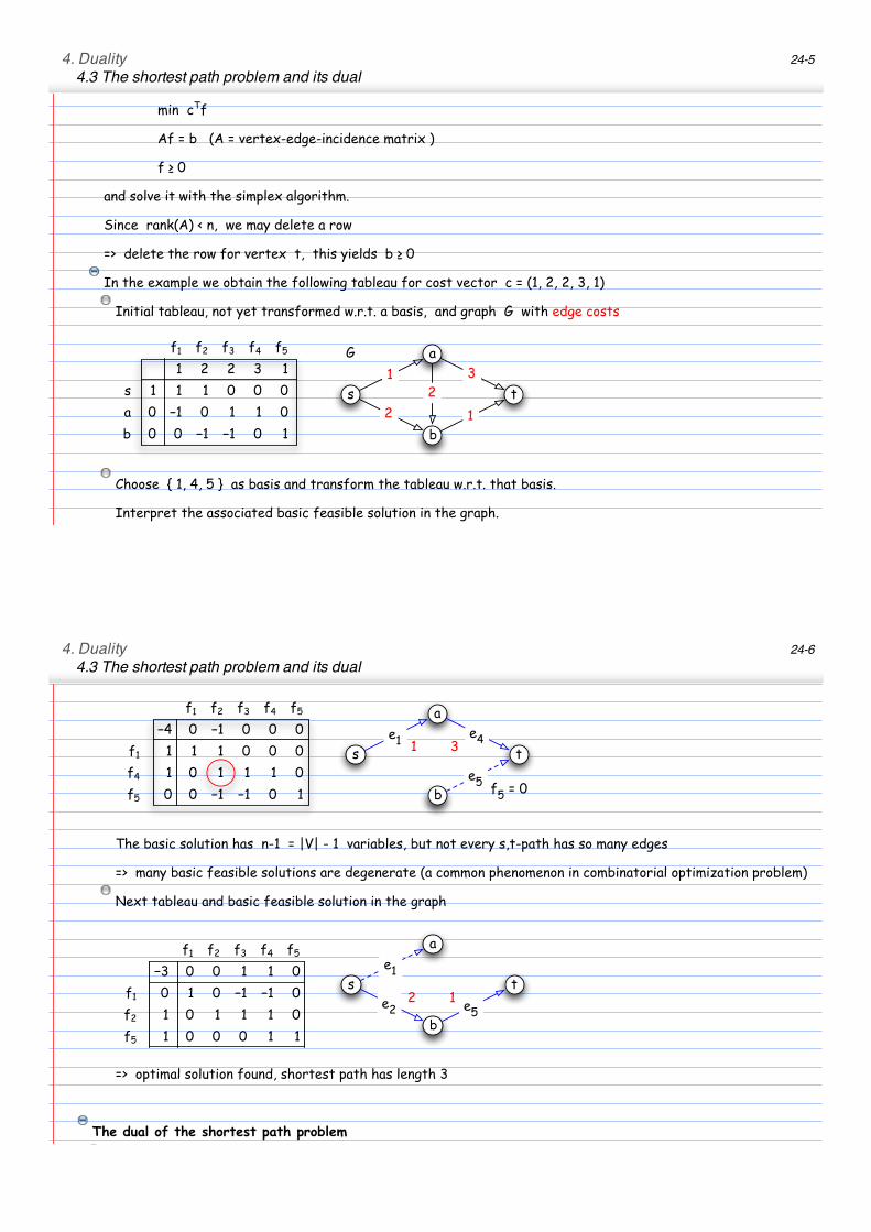
In the example we obtain the following tableau for cost vector c = (1, 2, 2, 3, 1)

Initial tableau, not yet transformed w.r.t. a basis, and graph G with edge costs

!! !" !# !$ !%

! " " # !

" ! ! ! & & &

# & !! & ! ! &

$ & & !! !! & !

s

a

b

t

1

2

2

3

1

G

Choose { 1, 4, 5 } as basis and transform the tableau w.r.t. that basis.

Interpret the associated basic feasible solution in the graph.


24-6

!! !" !# !$ !%

!$ & !! & & &

!! ! ! ! & & &

!$ ! & ! ! ! &

!% & & !! !! & !

s

a

b

t

e1

e4

e5

f5 = 0

1 3

The basic solution has n-1 = |V| - 1 variables, but not every s,t-path has so many edges

=> many basic feasible solutions are degenerate (a common phenomenon in combinatorial optimization problem)

Next tableau and basic feasible solution in the graph

!! !" !# !$ !%

!# & & ! ! &

!! & ! & !! !! &

!" ! & ! ! ! &

!% ! & & & ! !

s

a

b

t

e1

e2 e

5

2 1

=> optimal solution found, shortest path has length 3

The dual of the shortest path problem

We formulate it w.r.t. the full tableau containing also the row for vertex t


24-7

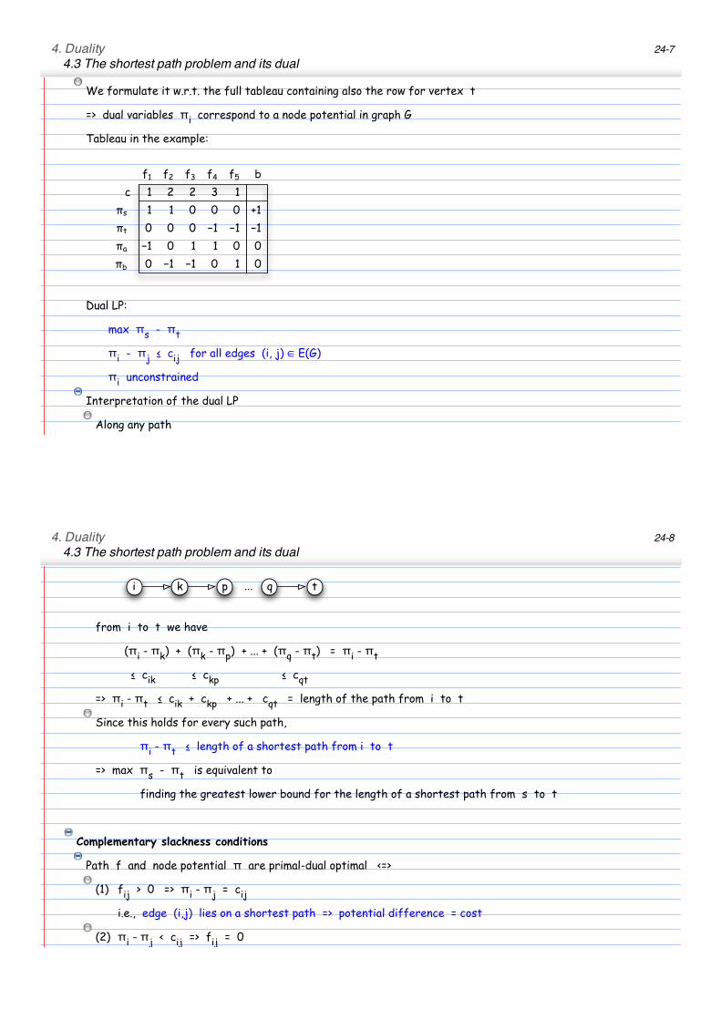
We formulate it w.r.t. the full tableau containing also the row for vertex t

=> dual variables πi correspond to a node potential in graph G

Tableau in the example:

!! !" !# !$ !% "

# ! " " # !

$% ! ! & & & '!

$& & & & !! !! !!

$' !! & ! ! & &

$" & !! !! & ! &

Dual LP:

max πs - πt

πi - πj " cij for all edges (i, j) ∈ E(G)

πi unconstrained

Interpretation of the dual LP

Along any path


24-8

i k p q t...

from i to t we have

(πi - πk) + (πk - πp) + ... + (πq - πt) = πi - πt

" cik " ckp " cqt

=> πi - πt " cik + ckp + ... + cqt = length of the path from i to t

Since this holds for every such path,

πi - πt " length of a shortest path from i to t

=> max πs - πt is equivalent to

finding the greatest lower bound for the length of a shortest path from s to t

Complementary slackness conditions

Path f and node potential π are primal-dual optimal <=>

(1) fij > 0 => πi - πj = cij

i.e., edge (i,j) lies on a shortest path => potential difference = cost

(2) πi - πj < cij => fij = 0

i.e., potential difference < cost => edge (i,j) does not lie on a shortest path


24-9

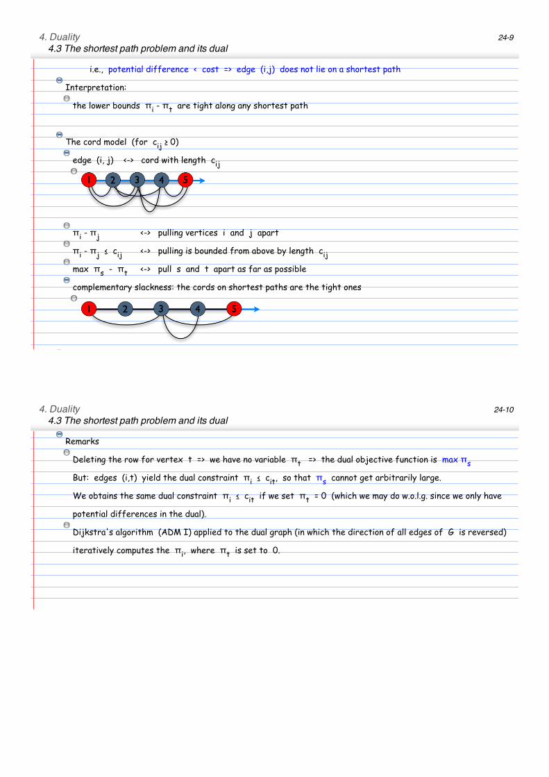
i.e., potential difference < cost => edge (i,j) does not lie on a shortest path

Interpretation:

the lower bounds πi - πt are tight along any shortest path

The cord model (for cij ! 0)

edge (i, j) <-> cord with length cij

πi - πj <-> pulling vertices i and j apart

πi - πj " cij <-> pulling is bounded from above by length cij

max πs - πt <-> pull s and t apart as far as possible

complementary slackness: the cords on shortest paths are the tight ones

Remarks


24-10

Remarks

Deleting the row for vertex t => we have no variable πt => the dual objective function is max πs

But: edges (i,t) yield the dual constraint πi " cit, so that πs cannot get arbitrarily large.

We obtains the same dual constraint πi " cit if we set πt = 0 (which we may do w.o.l.g. since we only have

potential differences in the dual).

Dijkstra's algorithm (ADM I) applied to the dual graph (in which the direction of all edges of G is reversed)

iteratively computes the πi, where πt is set to 0.

4. Duality4.4 Farkas' Lemma

25-1

This is a central and very useful lemma in duality theory. It has several variants also known as Theorems of the

Alternative.

Cones and projections

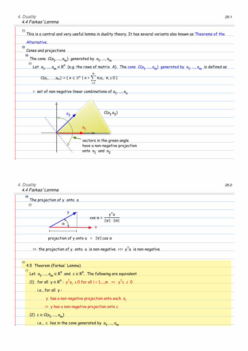
The cone C(a1, ..., am) generated by a1, ..., am

Let a1, ..., am ∈ Rn (e.g. the rows of matrix A). The cone C(a1, ..., am) generated by a1, ..., am is defined as

!!""# $ $ $ # "%# $% ! & ∈ R' " & %

%�

(%"

)("(# )( # & $

= set of non-negative linear combinations of a1, ..., an

vectors in the green angle have a non-negative projection onto a1 und a2

a2

a1

C(a1,a2)


25-2

The projection of y onto a

y

aα

!"#

�!� ! �#�cos α =

projection of y onto a = �!� cos α

=> the projection of y onto a is non-negative <=> yTa is non-negative

4.5 Theorem (Farkas' Lemma)

Let a1, ..., am ∈ Rn and c ∈ Rn. The following are equivalent

(1) for all y ∈ Rn : yTai ! 0 for all i = 1,...,m => yTc ! 0

i.e., for all y :

y has a non-negative projection onto each ai

=> y has a non-negative projection onto c

(2) c ∈ C(a1, ..., am)

i.e., c lies in the cone generated by a1, ..., am


25-3

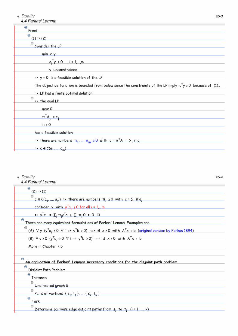
Proof

(1) => (2)

Consider the LP

min cTy

aiTy ! 0 i = 1,...,m

y unconstrained

=> y = 0 is a feasible solution of the LP

The objective function is bounded from below since the constraints of the LP imply cTy ! 0 because of (1),.

=> LP has a finite optimal solution

=> the dual LP

max 0

πTAj = cj

π ! 0

has a feasible solution

=> there are numbers π1, ..., πm ! 0 with c = πTA = #i πiai

=> c ∈ C(a1, ..., am)


25-4

(2) => (1)

c ∈ C(a1, ..., am) => there are numbers πi ! 0 with c = #i πiai

consider y with yTai ! 0 for all i = 1,...m

=> yTc = #i πiyTai ! #i πi·0 = 0 !

There are many equivalent formulations of Farkas' Lemma. Examples are

(A) ∀ y (yTai ! 0 ∀ i => yTb ! 0) <=> ∃ x ! 0 with ATx = b (original version by Farkas 1894)

(B) ∀ y ! 0 (yTai ! 0 ∀ i => yTb ! 0) <=> ∃ x ! 0 with ATx " b

More in Chapter 7.5

An application of Farkas' Lemma: necessary conditions for the disjoint path problem

Disjoint Path Problem

Instance

Undirected graph G

Pairs of vertices { s1, t1 }, ..., { sk, tk }

Task

Determine pairwise edge disjoint paths from si to ti (i = 1, ..., k)


25-5

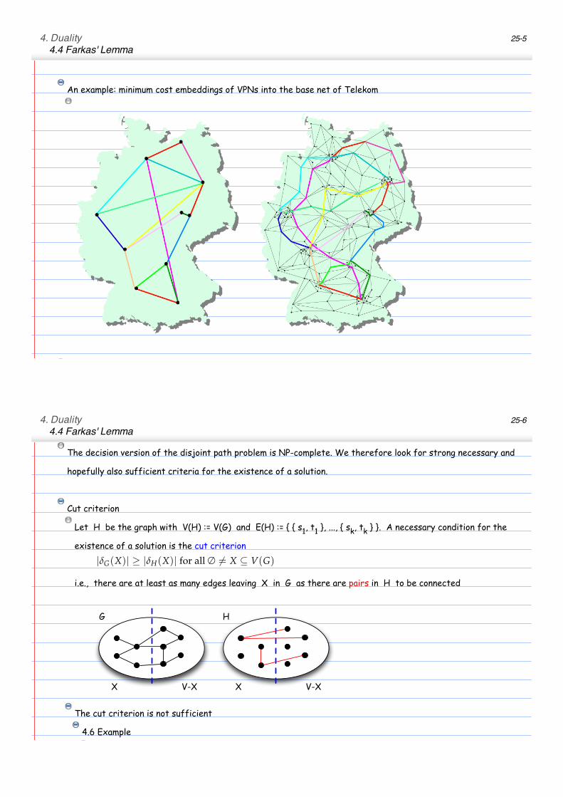
An example: minimum cost embeddings of VPNs into the base net of Telekom

The decision version of the disjoint path problem is NP-complete. We therefore look for strong necessary and


25-6

The decision version of the disjoint path problem is NP-complete. We therefore look for strong necessary and

hopefully also sufficient criteria for the existence of a solution.

Cut criterion

Let H be the graph with V(H) := V(G) and E(H) := { { s1, t1 }, ..., { sk, tk } }. A necessary condition for the

existence of a solution is the cut criterion

|δG(X)| ≥ |δH(X)| for all ∅ �= X ⊆ V(G)

i.e., there are at least as many edges leaving X in G as there are pairs in H to be connected

X V-X

G

V-X

X V-X

H

The cut criterion is not sufficient

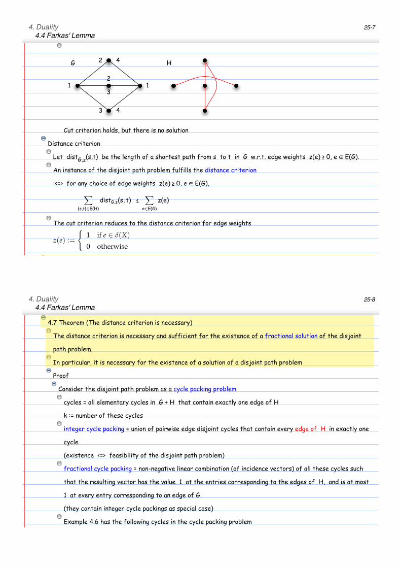
4.6 Example


25-7

1 1

3

2

3 4

2 4G H

Cut criterion holds, but there is no solution

Distance criterion

Let distG,z(s,t) be the length of a shortest path from s to t in G w.r.t. edge weights z(e) ! 0, e ∈ E(G).

An instance of the disjoint path problem fulfills the distance criterion

:<=> for any choice of edge weights z(e) ! 0, e ∈ E(G),

�

!!"#"∈$!%"

&'!#(")!!" #" #�

*∈$!("

)!*"

The cut criterion reduces to the distance criterion for edge weights

z(e) :=

�1 if e ∈ δ(X)

0 otherwise

4.7 Theorem (The distance criterion is necessary)


25-8

4.7 Theorem (The distance criterion is necessary)

The distance criterion is necessary and sufficient for the existence of a fractional solution of the disjoint

path problem.

In particular, it is necessary for the existence of a solution of a disjoint path problem

Proof

Consider the disjoint path problem as a cycle packing problem

cycles = all elementary cycles in G + H that contain exactly one edge of H

k := number of these cycles

integer cycle packing = union of pairwise edge disjoint cycles that contain every edge of H in exactly one

cycle

(existence <=> feasibility of the disjoint path problem)

fractional cycle packing = non-negative linear combination (of incidence vectors) of all these cycles such

that the resulting vector has the value 1 at the entries corresponding to the edges of H, and is at most

1 at every entry corresponding to an edge of G.

(they contain integer cycle packings as special case)

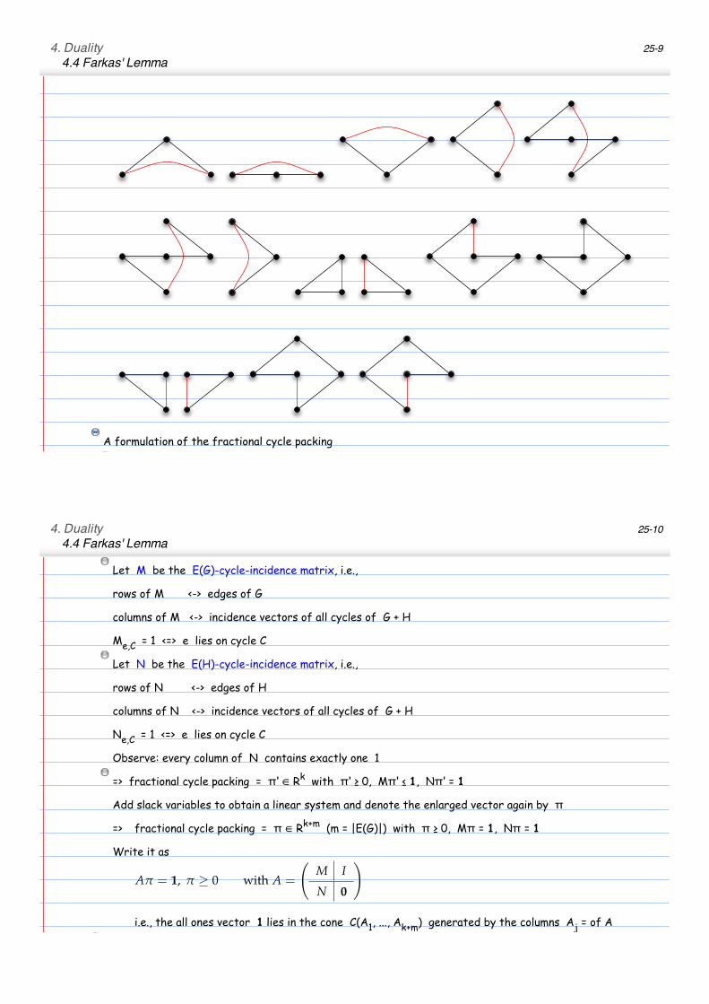
Example 4.6 has the following cycles in the cycle packing problem


25-9

A formulation of the fractional cycle packing

Let M be the E(G)-cycle-incidence matrix, i.e.,


25-10

Let M be the E(G)-cycle-incidence matrix, i.e.,

rows of M <-> edges of G

columns of M <-> incidence vectors of all cycles of G + H

Me,C = 1 <=> e lies on cycle C

Let N be the E(H)-cycle-incidence matrix, i.e.,

rows of N <-> edges of H

columns of N <-> incidence vectors of all cycles of G + H

Ne,C = 1 <=> e lies on cycle C

Observe: every column of N contains exactly one 1

=> fractional cycle packing = π' ∈ Rk with π' ! 0, Mπ' " 1, Nπ' = 1

Add slack variables to obtain a linear system and denote the enlarged vector again by π=> fractional cycle packing = π ∈ Rk+m (m = |E(G)|) with π ! 0, Mπ = 1, Nπ = 1

Write it as

Aπ = 1, π ≥ 0 with A =

�M I

N 0

�

i.e., the all ones vector 1 lies in the cone C(A1, ..., Ak+m) generated by the columns Aj = of A

Applying Farkas' Lemma gives condition (3)


25-11

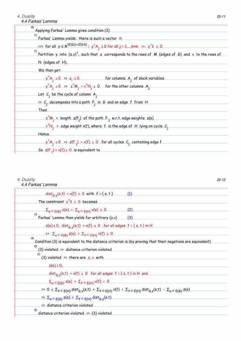
Applying Farkas' Lemma gives condition (3)

Farkas' Lemma yields: there is such a vector π<=> for all y ∈ R|E(G)|+|E(H)| : yTAj ! 0 for all j = 1,...,k+m => yT1 ! 0

Partition y into (z,v)T, such that z corresponds to the rows of M (edges of G) and v to the rows of

N (edges of H).

We then get:

yTAj ! 0 => zi ! 0 for columns Aj of slack variables

yTAj ! 0 => zTMj + vTNj ! 0 for the other columns Aj

Let Cj be the cycle of column Aj

=> Cj decomposes into a path Pj in G and an edge f from H

Then

zTMj = length z(Pj) of the path P j w.r.t. edge weights z(e)

vTNj = edge weight v(f), where f is the edge of H lying on cycle Cj

Hence

yTAj ! 0 => z(P j) + v(f) ! 0 for all cycles Cj containing edge f

So z(P j) + v(f) ! 0 is equivalent to

distG,z(s,t) + v(f) ! 0 with f = { s, t } (1)


25-12

distG,z(s,t) + v(f) ! 0 with f = { s, t } (1)

The constraint yT1 ! 0 becomes

#e ! E(G) z(e) + #e ! E(H) v(e) ! 0 (2)

Farkas' Lemma then yields for arbitrary (z,v) (3)

z(e) ! 0, distG,z(s,t) + v(f) ! 0 for all edges f = { s, t } in H

=> #e ! E(G) z(e) + #f ! E(H) v(f) ! 0

Condition (3) is equivalent to the distance criterion is (by proving that their negations are equivalent)

(3) violated => distance criterion violated

(3) violated => there are z, v with

z(e) ! 0,

distG,z(s,t) + v(f) ! 0 for all edges f = { s, t } in H and

#e ! E(G) z(e) + #f ! E(H) v(f) < 0

=> 0 " #f ! E(H) distG,z(s,t) + #f ! E(H) v(f) < #f ! E(H) distG,z(s,t) - #e ! E(G) z(e)

=> #e ! E(G) z(e) < #f ! E(H) distG,z(s,t)

=> distance criterion violated

distance criterion violated => (3) violated

distance criterion violated


25-13

distance criterion violated

=> there is z ! 0 with #e ! E(G) z(e) < #f ! E(H) distG,z(s,t)

choose v(f) := - distG,z(s,t) for edge f = {s, t} in H

=> distG,z(s,t) + v(f) ! 0 for all edges f = { s, t } in H and

#e ! E(G) z(e) + #f ! E(H) v(f) = #e ! E(G) z(e) - #f ! E(H) distG,z(s,t) < 0

=> (3) is violated !

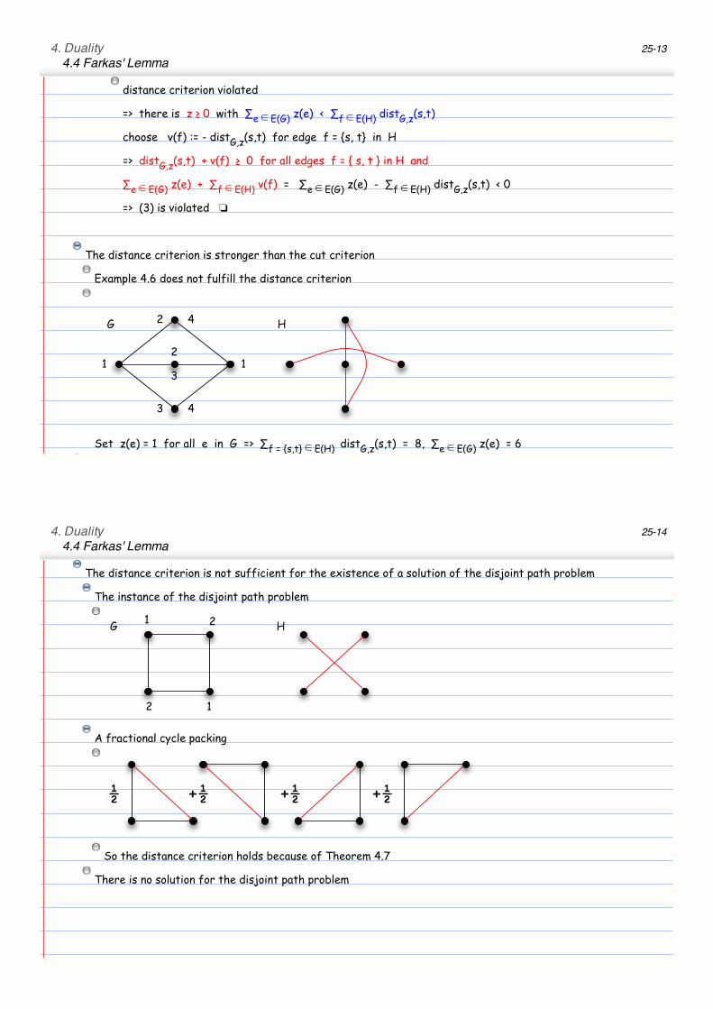
The distance criterion is stronger than the cut criterion

Example 4.6 does not fulfill the distance criterion

1 1

3

2

3 4

2 4G H

Set z(e) = 1 for all e in G => #f = {s,t} ! E(H) distG,z(s,t) = 8, #e ! E(G) z(e) = 6

The distance criterion is not sufficient for the existence of a solution of the disjoint path problem


25-14

The distance criterion is not sufficient for the existence of a solution of the disjoint path problem

The instance of the disjoint path problem

1

12

2G H

A fractional cycle packing

! +! +! +!

So the distance criterion holds because of Theorem 4.7

There is no solution for the disjoint path problem

4. Duality4.5 Dual information in the tableau

26-1

How to get dual information from the optimal primal tableau?

Suppose w.o.l.g. that the initial tableau (possibly with artificial variables from Phase I) has columns 1,...,m as

basic columns and that the tableau is transformed w.r.t. to this basis

1

1

...

Then the following properties hold in the optimal tableau with basis B

rows 1,...,m are obtained from the initial tableau by multiplying it with B-1 from the left

the reduced cost are obtained as!!" " !" ! #

$%" " # $%&&#'

where π is an optimal solution of the dual problem (Proof of the Strong Duality Theorem)

In columns 1,...,m (which are unit vectors in the initial tableau) we get!!" " !" ! #

$%" " !" ! #" #$&%%&

Hence an optimal dual solution is obtained from the optimal tableau of the primal as


26-2

!" ! #" ! "#" #" ! $$ % % % $ &% #&%$'%

Observe: this holds for the dual problem of the initial tableau (and not for dual versions of other, equivalent

primal formulations).

Moreover, the first m columns contain B-1 = B-1 I (4.13)

cj - !j

B-1

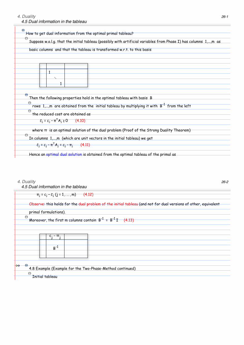
4.8 Example (Example for the Two-Phase-Method continued)

Initial tableau


26-3

!"!

!""

!"#

!! !" !# !$ !%

!# & & & & ! ! ! ! !

!$ & ! ! ! & & & & &

!"!

! ! & & # " ! & &

!""

# & ! & % ! ! ! &

!"#

$ & & ! " " ! & !

Optimal tableau

!"!

!""

!"#

!! !" !# !$ !%

!# !&$" %$" !! !! #$" ' #$" ' '

!% ' ! ! ! ' ' ' ' '

!" !$" !$" ' ' #$" ! !$" ' '

!$ %$" !!$" ! ' ($" ' !$" ! '

!% #$" !%$" ' ! !!!$" ' !!$" ' !

(4.12) gives π1 = 0 - 5/2 = - 5/2

π2 = 0 - (- 1) = 1

π3 = 0 - (- 1) = 1

for the values of the dual variables w.r.t. the dual problem obtained from the primal formulation with artificial


26-4

for the values of the dual variables w.r.t. the dual problem obtained from the primal formulation with artificial

variables xia

4.9 Example (Example for the shortest path problem continued)

Solving the primal problem

Initial tableau has no identity matrix, but 2 unit vectors

=> add one artificial variable in Phase I

!" #! #" ## #$ #%

!$ ! & & & & &

!% & ! " " # !

& !" ! ! ! ! & & &

" #$ & & !! & ! ! &

' #% & & & !! !! & !

Transform cost coefficients of ξ and z to reduced form (must become 0 for basic variables)


26-5

!" #! #" ## #$ #%

!$ !! & !! !! & & &

!% & & $ # & & &

& !" ! ! ! ! & & &

" #$ & & !! & ! ! &

' #% & & & !! !! & !

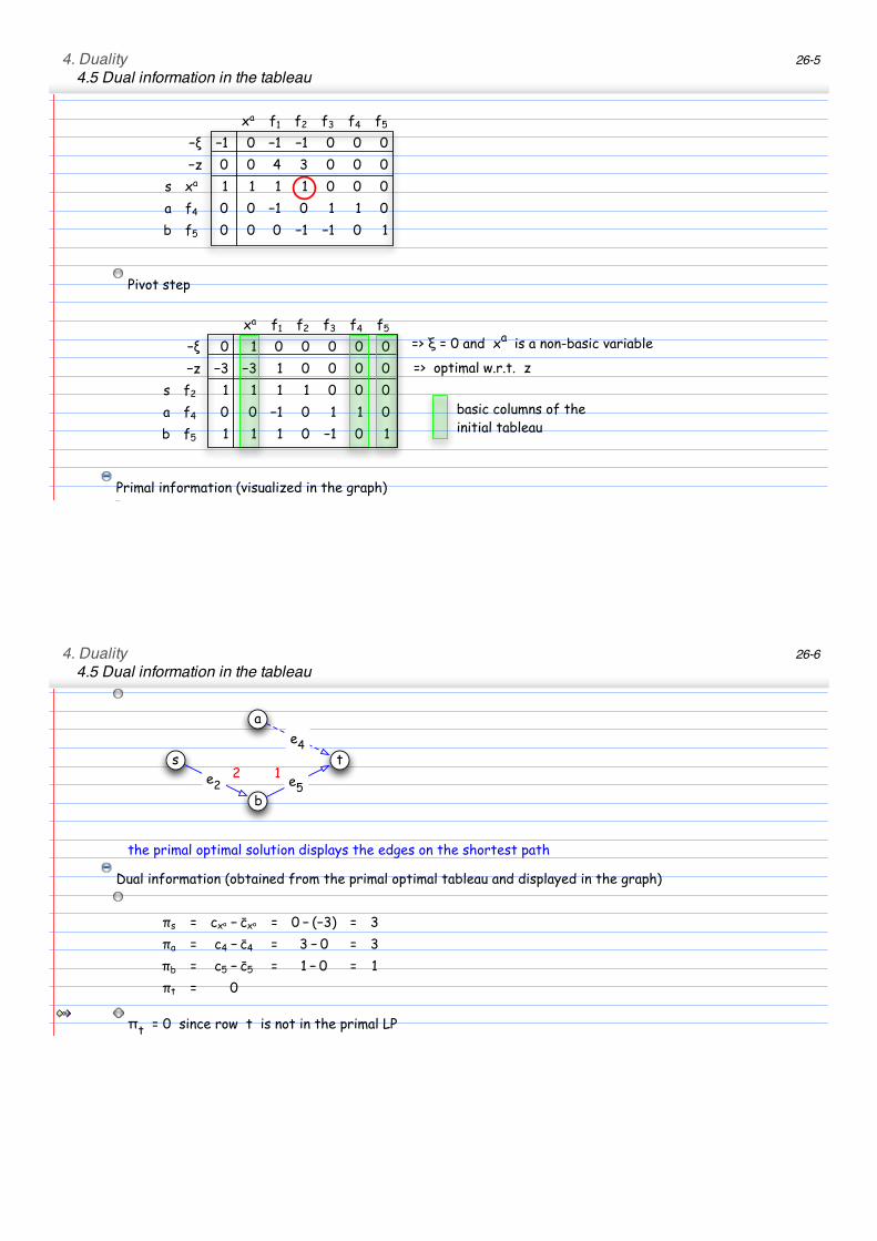
Pivot step

!" #! #" ## #$ #%

!$ & ! & & & & &

!% !# !# ! & & & &

& #" ! ! ! ! & & &

" #$ & & !! & ! ! &

' #% ! ! ! & !! & !

=> ξ = 0 and xa is a non-basic variable

=> optimal w.r.t. z

basic columns of the initial tableau

Primal information (visualized in the graph)


26-6

s

a

b

t

e2 e

5

2 1

e4

the primal optimal solution displays the edges on the shortest path

Dual information (obtained from the primal optimal tableau and displayed in the graph)

!" ! #$% ! "#$% ! # ! $!%& ! %

!% ! #' ! "#' ! % ! # ! %

!& ! #( ! "#( ! ) ! # ! )

!' ! #

πt = 0 since row t is not in the primal LP


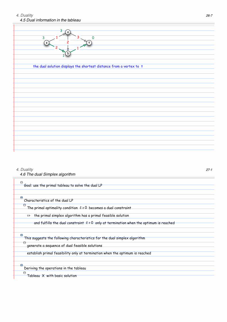
26-7

s

a

b

t

1

2

2

3

1

3

1

0

3

the dual solution displays the shortest distance from a vertex to t

4. Duality4.6 The dual Simplex algorithm

27-1

Goal: use the primal tableau to solve the dual LP

Characteristics of the dual LP

The primal optimality condition !! ! " becomes a dual constraint

=> the primal simplex algorithm has a primal feasible solution

and fulfills the dual constraint !! ! " only at termination when the optimum is reached

This suggests the following characteristics for the dual simplex algorithm

generate a sequence of dual feasible solutions

establish primal feasibility only at termination when the optimum is reached

Deriving the operations in the tableau

Tableau X with basic solution


27-2

!! !" !# !$ !%

!# ! & & & &

!" ! ! ! & & &

!$ ! & & & ! !

!# !! !! & ! & !!

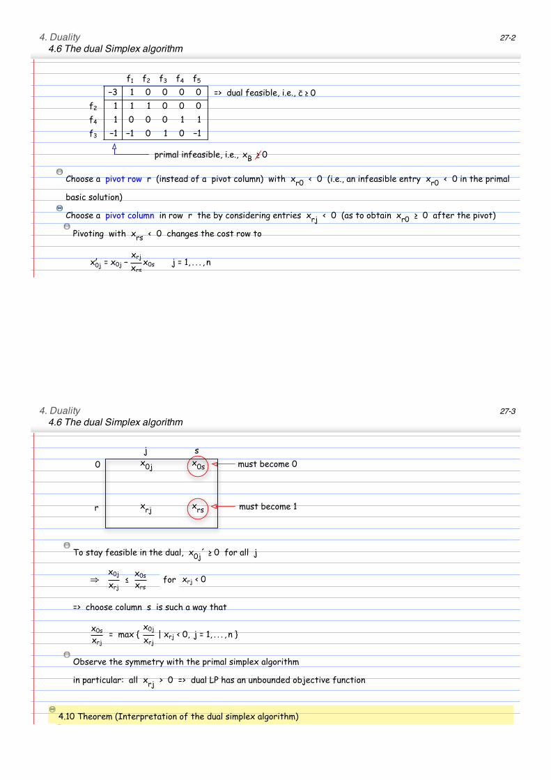
=> dual feasible, i.e.,

primal infeasible, i.e.,

!! ! "dual zulässig, d.h. !! ! "

nicht primal zulässig, d.h. xB ! 0

Choose a pivot row r (instead of a pivot column) with xr0 < 0 (i.e., an infeasible entry xr0 < 0 in the primal

basic solution)

Choose a pivot column in row r the by considering entries xrj < 0 (as to obtain xr0 ! 0 after the pivot)

Pivoting with xrs < 0 changes the cost row to

!�!" " !!" !

!#"

!#$!!$ " " #% & & & % '


27-3

0

r

j sx0j x0s

xrj xrs

must become 0

must become 1

To stay feasible in the dual, x0j´ ! 0 for all j

⇒!!"

!#"!

!!$

!#$"#$% !#" % !for

=> choose column s is such a way that

!!"

!#$" #$% !

!!$

!#$" !#$ % !& $ " && ' ' ' & ( #

Observe the symmetry with the primal simplex algorithm

in particular: all xrj > 0 => dual LP has an unbounded objective function

4.10 Theorem (Interpretation of the dual simplex algorithm)

The dual simplex algorithm is the primal simplex algorithm applied to the primal formulation of the dual LP


27-4

The dual simplex algorithm is the primal simplex algorithm applied to the primal formulation of the dual LP

Proof: Check !

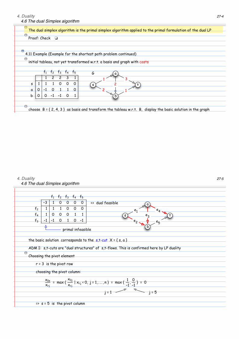
4.11 Example (Example for the shortest path problem continued)

initial tableau, not yet transformed w.r.t. a basis and graph with costs

!! !" !# !$ !%

! " " # !

" ! ! ! & & &

# & !! & ! ! &

$ & & !! !! & !

s

a

b

t

1

2

2

3

1

G

choose B = { 2, 4, 3 } as basis and transform the tableau w.r.t. B, display the basic solution in the graph


27-5

!! !" !# !$ !%

!# ! & & & &

!" ! ! ! & & &

!$ ! & & & ! !

!# !! !! & ! & !!

=> dual feasible

primal infeasible

s

a

b

t

e1

e2

e3

e4

e5

the basic solution corresponds to the s,t-cut X = { s, a }

ADM I: s,t-cuts are "dual structures" of s,t-flows. This is confirmed here by LP duality

Choosing the pivot element

r = 3 is the pivot row

choosing the pivot column:

!!"

!#$" #$% !

!!$

!#$" !#$ % !& $ " && ' ' ' & ( # " #$% !

&

$&&!

$&# " !

j = 1 j = 5

=> s = 5 is the pivot column


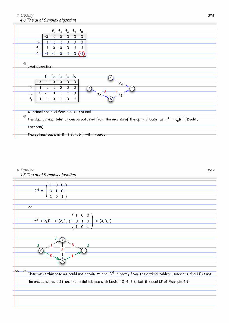
27-6

!! !" !# !$ !%

!# ! & & & &

!" ! ! ! & & &

!$ ! & & & ! !

!# !! !! & ! & !!

pivot operation

!! !" !# !$ !%

!# ! & & & &

!" ! ! ! & & &

!$ & !! & ! ! &

!% ! ! & !! & !

s

a

b

t

e2 e

5

2 1

e4

=> primal and dual feasible => optimal

The dual optimal solution can be obtained from the inverse of the optimal basis as !"! #

"

$$!"

(Duality

Theorem).

The optimal basis is B = { 2, 4, 5 } with inverse


27-7

!!!

"

! # #

# ! #

! # !

So

!" ! #"$$!" ! #$%%% "&

" ' '

' " '

" ' "

! #%%%% "&

s

a

b

t

1

2

2

3

1

3

1

0

3

Observe: in this case we could not obtain π and B-1 directly from the optimal tableau, since the dual LP is not

the one constructed from the initial tableau with basis { 2, 4, 3 }, but the dual LP of Example 4.9.

Documents

4. Duality 21 4.1 Duality of LPs and the duality theorem ...page.math.tu-berlin.de/~moehring/adm2/Chapter/chap4.pdf · 4.3 The shortest path problem and its dual ... 22-8 dual primal