Envelope Theorem, Euler, and Bellman Equations

without Differentiability∗

Ramon Marimon † Jan Werner ‡

February 15, 2015

Abstract

We extend the envelope theorem, the Euler equation, and the Bellman equation to dy-

namic constrained optimization problems where binding constraints can give rise to non-

differentiable value functions. The envelope theorem – an extension of Milgrom and Se-

gal (2002) theorem for concave functions – provides a generalization of the Euler equation

and establishes a relation between the Euler and the Bellman equation. For example, we

show how solutions to the standard Belllman equation may fail to satisfy the respective Euler

equations, in contrast with solutions to the infinite-horizon problem. In standard maximisa-

tion problems the failure of Euler equations may result in inconsistent multipliers, but not

in non-optimal outcomes. However, in problems with forward looking constraints this fail-

ure can result in inconsistent promises and non-optimal outcomes. We also show how the

inconsistency problem can be resolved by a minimal extension of the co-state. As an appli-

cation we extend the theory of recursive contracts of Marcet and Marimon (1998, 2015) to

the case where solutions are not unique, resolving a problem pointed out by Messner and

Pavoni (2004).

∗Preliminary draft. Do not quote without authors’ permission.†European University Institute, UPF-Barcelona GSE, CEPR and NBER‡University of Minnesota

1

1 Introduction

The Euler equation and the Bellman equation are the two basic tools to analyse dynamic prob-

lems. Euler equations are the first-order intert-temporal necessary conditions for optimal solu-

tions and, under standard concavity-convexity assumptions, they are also sufficient conditions,

provided that a transversality condition holds. Euler equations are second-order difference equa-

tions. The Bellman equation allows to transform an infinite-horizon optimisation problem into

a ‘two-periods-value’ problem, resulting in time independent policy functions determining the

actions as functions of the states. The Envelope Theorem provides the bridge between the Bell-

man equation and the Euler equations, confirming the necessity of the latter for the former, and

allowing to use Euler equations to obtain the policy functions of the Bellman equation. Further-

more, in deriving the Euler equations from the Bellman equation, the policy function reduces the

second-order difference equation system to first-order difference equations with corresponding

initial conditions, provided that the value function is differentiable.

Differentiability provides a tight bridge between the Bellman equation and the Euler equa-

tion. When the value function is differentiable, the state provides univocal information about its

derivative and, therefore, the inter-temporal change of values across states (Bellman) is uniquely

associated with the change of marginal values (Euler), and it is this tight bridge that allows for

the above described passage of properties between the Euler and the Bellman equations (e.g.

necessity and sufficiency in one direction and the additional structure of policy functions in the

other). Unfortunately, the bridge is no longer tight when the value function is not differentiable at

a given state. In this case, knowing the state and its value does not provide univocal information

about its derivative. Sub-differential calculus (e.g. Rockafellar (1970, 1981)) comes into play,

but needs to be properly developed to characterise the Envelope bridge between the Euler and

Bellman equations, without differentiability. This is the objective of this paper.

Recursive methods have been widely applied – particularly, in macroeconomics – in the last

25 years (e.g. since the publication of Stokey et al. (1989)) using the standard framework where

assumptions, such as interiority of optimal paths, imply the differentiability of the value function.

However, the differentiability issue cannot be ignored in a wide range of current applications. For

example, even if the underlying functions describing the model (e.g. preferences and technol-

ogy) are differentiable, value functions are not differentiable in many contractual and dynamic

2

problems when constraints are binding. Models where household, firms, or countries, may face

binding constraints in equilibrium are, nowadays, more the norm than the exception: in partic-

ular, when forward-looking constraints (i.e. constraints involving future equilibrium outcomes)

are part of the decision process. We focus our analysis on differentiability problems arising from

binding constraints.

Our analysis covers the trilogy already mentioned. First, the envelope theorem for constrained

optimisation problems without without assuming differentiability of the value function or interi-

ority of the solutions. We generalise the envelope theorem of Milgrom and Segal (2002, Corol-

lary 5) by dropping the concavity assumptions and weakening the Slater’s condition which they

assumed. Further, we extend it to multidimensional parameters. The theorem provides a char-

acterisation of directional derivatives, as well as sufficient conditions for the differentiability of

the value function; for example, If there is a unique saddle point, the value function is differen-

tiable and the standard form of the envelope theorem holds. Furthermore, If the value function is

concave or convex, the envelope theorem can be stated using the superdifferentials or the subd-

ifferential. We provide a characterizations of the superdifferential of the concave value function

and the subdifferential of the convex value function. A sufficient condition for differentiability

of the concave value function is that the saddle-point multiplier be unique. This extends the well

known result of Benveniste and Scheinkman (1979) which requires an interior solution implying

that zero is the unique multiplier. For the convex value function, a sufficient condition for dif-

ferentiability is that the solution is unique. We provide examples of applications of our results

to static optimization problems. This first part, which also contributes to the static theory of

constrained optimisation, is covered in Sections 2 to 5.

Second, we turn to the Euler equation – the first-order inter-temporal condition of the infinite-

horizon problem. Unless the solution is interior, the marginal value of the constraint must be part

of the Euler equation. The marginal value is well defined if and only if the value function is dif-

ferentiable at the chosen, or ‘variable’, state. Euler equations hold for a sequence {x∗t , λ∗t}∞t=0 that

includes uniquely defined multipliers λ∗t . If the value function is differentiable, Euler equations

have recursive representation. In fact, since the multipliers are uniquely defined, the recursive

representation is given by a policy function of the corresponding recursive problem. In the case

of interior solutions the problem of the lack of recursivity of the Euler equation does not arise, but

it does in the non-differentiable case. We apply the envelope theorem without differentiability to

3

generalize the characterization of optimal solutions using Euler equations when the value function

may not be differentiable. In general, this charcterization is not recursive, as it is in the varia-

tional problem, starting from the initial x0. In the latter, the inter-temporal Euler equations result

in ‘consistent’ selections of multipliers. However, if following the optimal path {x0, x∗1, . . . x

∗n}

a new optimisation is started, the state x∗n does not provide information of the previously selected

multipliers using the envelope theorem without differentiability. Nevertheless, when constraints

do not involve future outcomes, this ‘inconsistency’ only affects the multipliers: the saddle-point

solutions {x∗t}∞t=0 are optimal, even if the optimisation is re-started at some state. Section 6

contains this analysis and discussion.

Finally, we further develop the Bellman equation, or more precisely, the saddle-point Bellman

equation of recursive contracts of Marcet and Marimon (1998, 2015) for dynamic optimisation

problems with forward looking constraints. First, we show that, when the inter-temporal con-

straints are time-separable, using the ‘recursive contracts’approach, for one-period forward look-

ing constraints, one can have a well defined saddle-point Bellman equation. Second, we show

why for long-term forward looking constraints the ‘inconsistency problem’, discussed in the pre-

vious section can have an effect on outcomes – not just multipliers – resulting in non-optimal

solutions to the saddle-point Bellman equation. Messner and Pavoni (2004) provided an example

showing that recursive contracts with non-unique outcomes could deliver non-optimal solutions

(uniqueness is assumed in Marcet and Marimon (1998, 2011)), what we show here that the root

of this problem lies in the ‘inconsistency problem’. Finally, and more importantly, we show

that applying again the ‘recursive contracts’method of expanding the co-state, it is possible ob-

tain a new saddle-point Bellman equation where the recursive solution results in ‘consistent’Euler

equations; that is, a solution generated by this general saddle-point Bellman equation is a solution

to the original infinite-horizon problem, even if this solution is re-started at la later (expanded)

state. We conclude Section 7 with theorem the corresponding theorem that generalizes ‘recursive

contracts’to models with non-unique solutions.

Finally, it should be noticed that extensions of the envelope theorem have been developed in

recent years for the use in optimization problems with incentive constraints and/or non-convexities.

Rincon-Zapatero and Santos (2009) study differentiability of the value function in dynamic opti-

mization problems under the assumption that the value function is concave. Morand, Reffett and

Tarafdar (2011) study generalized differentiability of the value function and the envelope theo-

4

rem in non-smooth optimization problems1. Although the Euler equation is part of the standard

toolkit of dynamic optimization problems (e.g. Stokey et al. 1989), we are not aware of any

discussion of the recursively problem presented here. As said, this is possibly due to the fact that

most of the analysis, and computations, with Euler equations implicitly assume that the value

function is differentiable2. We have already explained the structure of the paper; all proves have

been relegated to the Appendix.

2 The Envelope Theorem

We consider the following parametric constrained optimization problem:

maxy∈Y

f(x, y) (1)

subject to

h1(x, y) ≥ 0, . . . , hk(x, y) ≥ 0. (2)

Parameter x lies in the set X ⊂ <m. Choice variable y lies in Y ⊂ <n. Objective function f is a

real-valued function on Y ×X. Each constraint functions hi is a real-valued function on Y ×X.3

We shall impose the following conditions

A1. Y is convex and compact; X is convex.

A2. f and hi are continuous functions of (x, y), for every i.

A3. For every x and every i, there exists yi ∈ Y such that hi(x, yi) > 0 and hj(x, yi) ≥ 0 for

j 6= i.

Assumptions A1-2 are standard. Assumption A3 essentially says that none of the inequality

constraints hi(x, y) ≥ 0 alone can be replaced by equality constraint hi(x, y) = 0. It is weaker

1Other contributions include Bonnisseau and Le Van (1996) and Clausen and Straub (2011).2A recent, and limited, solution to the recursive contracts’ uniqueness problem has been offered by Cole and

Kubler (2012).3Note that optimization problems with equality constraints can be represented in form (1–2) by taking hi = −hj

for some i and j.

5

than the Slater’s condition which requires that there is y ∈ Y such that hi(x, y) > 0 for every i.

If all functions hi are concave in y, then A3 is equivalent to the Slater’s condition.

Let V (x) denote the value function of the problem (1–2). The Lagrangian function associated

with (1–2) is

L(x, y, λ) = f(x, y) + λh(x, y), (3)

where λ ∈ <k+ is a vector of (positive) multipliers4. It is well-known that if (y∗, λ∗) is a saddle

point of L, that is, if

L(x, y, λ∗) ≤ L(x, y∗, λ∗) ≤ L(x, y∗, λ), (4)

for every y ∈ Y and λ ∈ <k+, then y∗ is a solution to (1–2). Further, the slackness condition,

λ∗h(x, y∗) = 0, holds and consequently

V (x) = L(x, y∗, λ∗). (5)

The set of saddle points of L at x is a product of two sets and is denoted by Y ∗(x) × Λ∗(x)

where Y ∗(x) ⊂ Y and Λ∗(x) ⊂ <k+, see Rockafellar (1970), Lemma 36.2. If (y∗, λ∗) is a

saddle point of L, y∗ will be called saddle-point solution and λ∗ a saddle-point multiplier. The

slackness condition implies that if the ith constraint is not binding, that is, hi(x, y∗) > 0 for some

y∗ ∈ Y ∗(x), then λ∗i = 0 for every λ∗ ∈ Λ∗(x). The set of saddle-point solutions Y ∗(x) is a subset

of the set of solutions to (1–2). If functions f and hi are concave in y and the Slater’s condition

holds, then the two sets are equal. If functions f and hi are differentiable in y, then the Kuhn-

Tucker first-order conditions hold for every saddle point of L. The set of saddle-point multipliers

Λ∗ is a subset of the set of Kuhn-Tucker multipliers. If functions f and hi are differentiable and

concave in y, those two sets are equal.

The envelope theorem is best stated in terms of directional derivatives. We first consider one-

dimensional parameter set X – a convex set on the real line. Directional derivatives are then the

left- and right-hand derivatives. The right- and left-hand derivatives of the value function V at x

are

V ′(x+) = limt→0+

V (x+ t)− V (x)

t, (6)

and

V ′(x−) = limt→0−

V (x+ t)− V (x)

t, (7)

4We use the product notation: λh(x, y) =∑k

i=1 λihi(x, y).

6

if the limits exist.

We have the following result:

Theorem 1: Suppose that X ⊂ <, conditions A1-A3 hold, and partial derivatives ∂f∂x

and ∂hi∂x

are

continuous functions of (x, y). Then the value function V is right- and left-hand differen-

tiable and the directional derivatives at x ∈ intX are

V ′(x+) = maxy∗∈Y ∗(x)

minλ∗∈Λ∗(x)

[∂f∂x

(x, y∗) + λ∗∂h

∂x(x, y∗)

](8)

and

V ′(x−) = miny∗∈Y ∗(x)

maxλ∗∈Λ∗(x)

[∂f∂x

(x, y∗) + λ∗∂h

∂x(x, y∗)

], (9)

where the order of maximum and minimum does not matter.

Theorem 1 is a extension of Corollary 5 in Milgrom and Segal (2002). It is worth pointing

out that differentiability of functions f and hi with respect to the variable y is not assumed in

Theorem 1. This will be important in applications to recursive dynamic problems in Section 7.

For a multi-dimensional parameter set X in <m, the directional derivative of the value func-

tion V at x ∈ X in the direction x ∈ <m such that x+ x ∈ X is defined as

V ′(x; x) = limt→0+

V (x+ tx)− V (x)

t.

If partial derivatives of V exist, then the directional derivative V ′(x; x) is equal to the scalar

product DV (x)x, where DV (x) is the vector of partial derivatives, i.e., the gradient vector.

Theorem 1 can be applied to the single-variable value function V (t) ≡ V (x + tx) for which

it holds V ′(0+) = V ′(x; x). If Dxf(x, y) and Dxhi(x, y) are continuous functions of (x, y), then

it follows that the directional derivative of V is

V ′(x; x) = maxy∗∈Y ∗(x)

minλ∗∈Λ∗(x)

[Dxf(x, y∗) + λ∗Dxh(x, y∗)

]x, (10)

and the order of maximum and minimum does not matter.

3 Differentiability of the Value Function

The value function V on X ⊂ < is differentiable at x if the one-sided derivatives are equal to

each other. Sufficient conditions for differentiability can be obtained from Theorem 1.

7

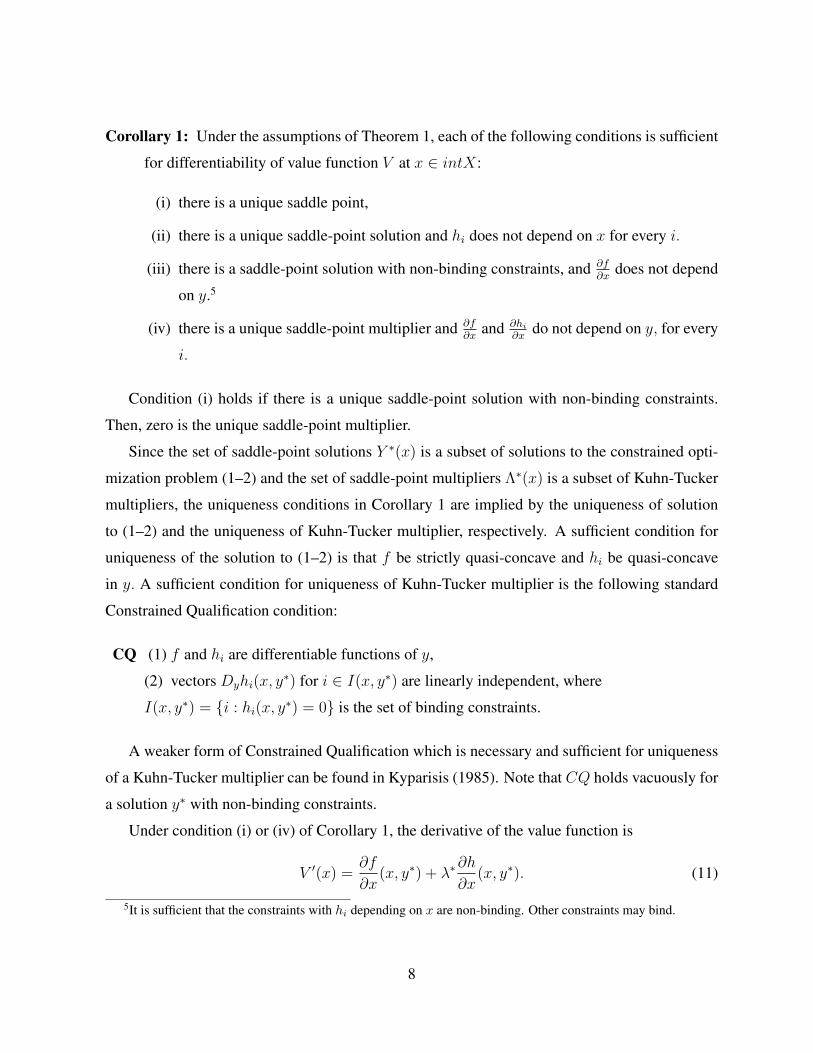
Corollary 1: Under the assumptions of Theorem 1, each of the following conditions is sufficient

for differentiability of value function V at x ∈ intX:

(i) there is a unique saddle point,

(ii) there is a unique saddle-point solution and hi does not depend on x for every i.

(iii) there is a saddle-point solution with non-binding constraints, and ∂f∂x

does not depend

on y.5

(iv) there is a unique saddle-point multiplier and ∂f∂x

and ∂hi∂x

do not depend on y, for every

i.

Condition (i) holds if there is a unique saddle-point solution with non-binding constraints.

Then, zero is the unique saddle-point multiplier.

Since the set of saddle-point solutions Y ∗(x) is a subset of solutions to the constrained opti-

mization problem (1–2) and the set of saddle-point multipliers Λ∗(x) is a subset of Kuhn-Tucker

multipliers, the uniqueness conditions in Corollary 1 are implied by the uniqueness of solution

to (1–2) and the uniqueness of Kuhn-Tucker multiplier, respectively. A sufficient condition for

uniqueness of the solution to (1–2) is that f be strictly quasi-concave and hi be quasi-concave

in y. A sufficient condition for uniqueness of Kuhn-Tucker multiplier is the following standard

Constrained Qualification condition:

CQ (1) f and hi are differentiable functions of y,

(2) vectors Dyhi(x, y∗) for i ∈ I(x, y∗) are linearly independent, where

I(x, y∗) = {i : hi(x, y∗) = 0} is the set of binding constraints.

A weaker form of Constrained Qualification which is necessary and sufficient for uniqueness

of a Kuhn-Tucker multiplier can be found in Kyparisis (1985). Note that CQ holds vacuously for

a solution y∗ with non-binding constraints.

Under condition (i) or (iv) of Corollary 1, the derivative of the value function is

V ′(x) =∂f

∂x(x, y∗) + λ∗

∂h

∂x(x, y∗). (11)

5It is sufficient that the constraints with hi depending on x are non-binding. Other constraints may bind.

8

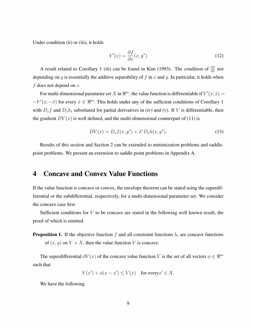
Under condition (ii) or (iii), it holds

V ′(x) =∂f

∂x(x, y∗) (12)

A result related to Corollary 1 (iii) can be found in Kim (1993). The condition of ∂f∂x

not

depending on y is essentially the additive separability of f in x and y. In particular, it holds when

f does not depend on x.

For multi-dimensional parameter setX in<m, the value function is differentiable if V ′(x; x) =

−V ′(x;−x) for every x ∈ <m. This holds under any of the sufficient conditions of Corollary 1

with Dxf and Dxhi substituted for partial derivatives in (iv) and (v). If V is differentiable, then

the gradient DV (x) is well defined, and the multi-dimensional counterpart of (11) is

DV (x) = Dxf(x, y∗) + λ∗Dxh(x, y∗). (13)

Results of this section and Section 2 can be extended to minimization problems and saddle-

point problems. We present an extension to saddle-point problems in Appendix A.

4 Concave and Convex Value Functions

If the value function is concave or convex, the envelope theorem can be stated using the superdif-

ferential or the subdifferential, respectively, for a multi-dimensional parameter set. We consider

the concave case first.

Sufficient conditions for V to be concave are stated in the following well known result, the

proof of which is omitted.

Proposition 1. If the objective function f and all constraint functions hi are concave functions

of (x, y) on Y ×X, then the value function V is concave.

The superdifferential ∂V (x) of the concave value function V is the set of all vectors φ ∈ <m

such that

V (x′) + φ(x− x′) ≤ V (x) for everyx′ ∈ X.

We have the following

9

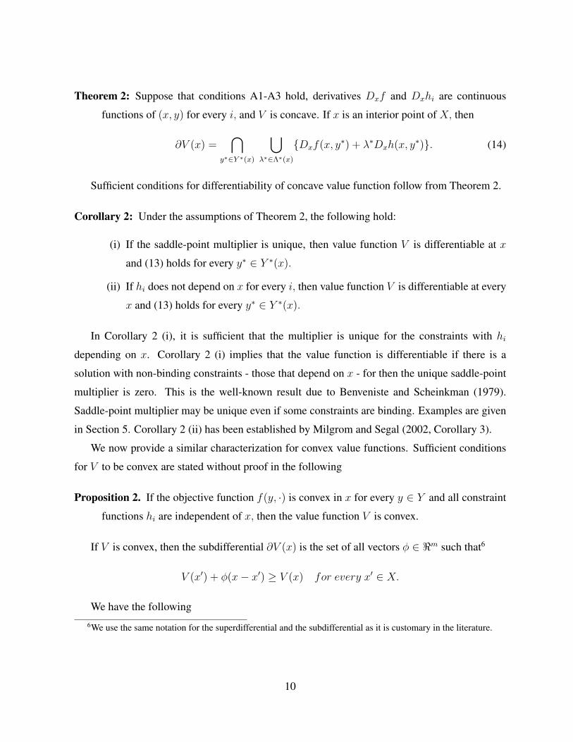
Theorem 2: Suppose that conditions A1-A3 hold, derivatives Dxf and Dxhi are continuous

functions of (x, y) for every i, and V is concave. If x is an interior point of X, then

∂V (x) =⋂

y∗∈Y ∗(x)

⋃λ∗∈Λ∗(x)

{Dxf(x, y∗) + λ∗Dxh(x, y∗)}. (14)

Sufficient conditions for differentiability of concave value function follow from Theorem 2.

Corollary 2: Under the assumptions of Theorem 2, the following hold:

(i) If the saddle-point multiplier is unique, then value function V is differentiable at x

and (13) holds for every y∗ ∈ Y ∗(x).

(ii) If hi does not depend on x for every i, then value function V is differentiable at every

x and (13) holds for every y∗ ∈ Y ∗(x).

In Corollary 2 (i), it is sufficient that the multiplier is unique for the constraints with hi

depending on x. Corollary 2 (i) implies that the value function is differentiable if there is a

solution with non-binding constraints - those that depend on x - for then the unique saddle-point

multiplier is zero. This is the well-known result due to Benveniste and Scheinkman (1979).

Saddle-point multiplier may be unique even if some constraints are binding. Examples are given

in Section 5. Corollary 2 (ii) has been established by Milgrom and Segal (2002, Corollary 3).

We now provide a similar characterization for convex value functions. Sufficient conditions

for V to be convex are stated without proof in the following

Proposition 2. If the objective function f(y, ·) is convex in x for every y ∈ Y and all constraint

functions hi are independent of x, then the value function V is convex.

If V is convex, then the subdifferential ∂V (x) is the set of all vectors φ ∈ <m such that6

V (x′) + φ(x− x′) ≥ V (x) for every x′ ∈ X.

We have the following

6We use the same notation for the superdifferential and the subdifferential as it is customary in the literature.

10

Theorem 3: Suppose that conditions A1-A3 hold, derivatives Dxf and Dxhi are continuous

functions of (x, y) for every i, and V is convex. If x is an interior point of X, then

∂V (x) =⋂

λ∗∈Λ∗(x)

co( ⋃y∗∈Y ∗(x)

{Dxf(x, y∗) + λ∗Dxh(x, y∗)}), (15)

where co( ) denotes the convex hull.

Sufficient conditions for differentiability of convex value function follow from Theorem 3.

Corollary 3: Under the assumptions of Theorem 3, if the saddle-point solution is unique, then

value function V is differentiable at x and (13) holds for every y∗ ∈ Y ∗(x).

5 Examples

Example 1 (Perturbation of constraints): Suppose that the objective function f in (1) is inde-

pendent of the parameter x and constraint functions are of the form hi(x, y) = hi(y) − xi. This

optimization problem is a perturbation of the non-parametric problem with objective function f

and constraint functions hi. Rockafellar (1970) provides an extensive discussion of the concave

perturbed problem.

Corollary 1 (iv) implies that if the saddle-point multiplier λ∗ is unique, then the value function

is differentiable and DV (x) = −λ∗ by (13). (See 29.1.3 in Rockafellar (1970) for the concave

perturbed problem.) If f and hi are concave for every i, then V is concave and the superdifferen-

tial of V is ∂V (x) = −Λ∗(x).

Example 2 (A planner’s problem): Consider the resource allocation problem in an economy

with k agents. The planner’s problem is

max{ci}

k∑i=1

µiui(ci) (16)

s.t.n∑i=1

ci ≤ x, (17)

ci ≥ 0, ∀i,

11

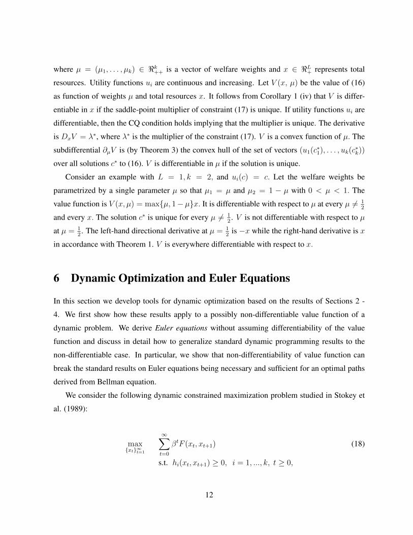
where µ = (µ1, . . . , µk) ∈ <k++ is a vector of welfare weights and x ∈ <L+ represents total

resources. Utility functions ui are continuous and increasing. Let V (x, µ) be the value of (16)

as function of weights µ and total resources x. It follows from Corollary 1 (iv) that V is differ-

entiable in x if the saddle-point multiplier of constraint (17) is unique. If utility functions ui are

differentiable, then the CQ condition holds implying that the multiplier is unique. The derivative

is DxV = λ∗, where λ∗ is the multiplier of the constraint (17). V is a convex function of µ. The

subdifferential ∂µV is (by Theorem 3) the convex hull of the set of vectors (u1(c∗1), . . . , uk(c∗k))

over all solutions c∗ to (16). V is differentiable in µ if the solution is unique.

Consider an example with L = 1, k = 2, and ui(c) = c. Let the welfare weights be

parametrized by a single parameter µ so that µ1 = µ and µ2 = 1 − µ with 0 < µ < 1. The

value function is V (x, µ) = max{µ, 1−µ}x. It is differentiable with respect to µ at every µ 6= 12

and every x. The solution c∗ is unique for every µ 6= 12. V is not differentiable with respect to µ

at µ = 12. The left-hand directional derivative at µ = 1

2is −x while the right-hand derivative is x

in accordance with Theorem 1. V is everywhere differentiable with respect to x.

6 Dynamic Optimization and Euler Equations

In this section we develop tools for dynamic optimization based on the results of Sections 2 -

4. We first show how these results apply to a possibly non-differentiable value function of a

dynamic problem. We derive Euler equations without assuming differentiability of the value

function and discuss in detail how to generalize standard dynamic programming results to the

non-differentiable case. In particular, we show that non-differentiability of value function can

break the standard results on Euler equations being necessary and sufficient for an optimal paths

derived from Bellman equation.

We consider the following dynamic constrained maximization problem studied in Stokey et

al. (1989):

max{xt}∞t=1

∞∑t=0

βtF (xt, xt+1) (18)

s.t. hi(xt, xt+1) ≥ 0, i = 1, ..., k, t ≥ 0,

12

where xt ∈ X ⊂ <n for every t, and x0 is given. Functions F and hi are real-valued functions

on X ×X . In addition to assumptions A1 - A3, we impose the following conditions:

A4. F and hi are bounded, and β ∈ (0, 1).

A5. F and hi are concave functions of (x, y) on X ×X,

A.6. F and hi are increasing and continuously differentiable.

The saddle-point problem associated with (18) is

max{xt}∞t=1

min{λt}∞t=1,λt≥0,

∞∑t=0

βt[F (xt, xt+1) + λt+1h(xt, xt+1)

], (19)

As it is well known7, if sequence {x∗t} is a solution to (18), then under assumptions A1-A5 there

exist multipliers {λ∗t} such that {x∗t , λ∗t} is a saddle-point of (19). Furthermore, without any

assumptions, if {x∗t , λ∗t} is a saddle-point of (19) then {x∗t} is a solution to (18).

Under assumptions A1-A6, the first-order necessary conditions for saddle-point {x∗t , λ∗t} are

the following intertemporal Euler equations

DyF (x∗t , x∗t+1) + λ∗t+1Dyh(x∗t , x

∗t+1) + β

[DxF (x∗t+1, x

∗t+2) + λ∗t+2Dxh(x∗t+1, x

∗t+2)]

= 0, (20)

for every t ≥ 0. Equations (20) together with complementary slackness conditions

λ∗i,t+1hi(x∗t , x∗t+1) = 0, (21)

and the constraints hi(x∗t , x∗t+1) ≥ 0 for every t can be considered as a system of second-order

difference equations for the sequence {x∗t , λ∗t} with x∗0 = x0. For an interior solution, with

hi(x∗t , x∗t+1) > 0 for every t ≥ 0, equations (20) simplify to the standard Euler equations

DyF (x∗t , x∗t+1) + β

[DxF (x∗t+1, x

∗t+2)]

= 0. (22)

The sufficiency of the Euler equations and a transversality condition, see Stokey et al. (1989),

continues to hold for non-interior solutions.7See, for example, Luenberger (1969) Theorems 8.3 and 8.4.2.

13

Proposition 3: Suppose that conditions A1-A6 hold. Let {x∗t , λ∗t}, with x∗0 = x0 and λ∗t ≥ 0 for

every t, satisfy the Euler equations (20) and (21). If the transversality condition

limt→∞

βt[DxF (x∗t , x

∗t+1) + λ∗t+1Dxh(x∗t , x

∗t+1)

]x∗t = 0, (23)

holds, then {x∗t} is a solution to (18).

Proof: see Appendix.

Let V (x0) be the value function of (18). The value function satisfies the Bellman equation

V (x) = maxy

{F (x, y) + βV (y)} (24)

s.t. hi(x, y) ≥ 0, i = 1, ..., k (25)

For every solution {x∗t} to (18), x∗t+1 is a solution to Bellman equation (25) at x∗t . The converse

holds as well under assumption A4, see Stokey et al. (1989). As in Section 2, we shall consider

saddle-points of the Lagrangian associated with the maximization problem on the right-hand side

of Bellman equation. We shall refer to these as saddle-points of Bellman equation, for short.

Value function V is concave under assumption A5. The superdifferential of V is, by Theorem

2,

∂V (x) =⋂

y∗∈Y ∗(x)

⋃λ∗∈Λ∗(x)

[DxF (x, y∗) + λ∗Dxh(x, y∗)

](26)

where Y ∗(x) is the set of saddle-point solutions and Λ∗(x) is the set of saddle-point multipliers

of the constraints (25) at x.

Corollary 2 (i) implies that V is differentiable if the multiplier λ∗ is unique. Note that the

constrained qualification CQ cannot be used to assert uniqueness of the multiplier since the ob-

jective function in (24) may not be differentiable in y. However, if there is a solution y∗ with

non-binding constraints, then the unique multiplier is zero and V is differentiable at x; this is the

well known result of Benveniste and Scheinkman (1979).

We discuss now the validity of the Euler equations for a sequence of saddle-point solutions

to the Bellman equation. Consider a sequence {x∗t , λ∗t} such that (x∗t+1, λ∗t+1) is a saddle-point of

Bellman equation at x∗t . If assumptions A1-A4 hold, then the first-order condition for (x∗t+1, λ∗t+1)

is

DyF (x∗t , x∗t+1) + λ∗t+1Dyh(x∗t , x

∗t+1) + βφ∗t+1 = 0, (27)

14

for some φ∗t+1 ∈ ∂V (x∗t+1), see Rockafellar (1981, Ch.5). The envelope representation (26) of

∂V (x∗t+1) implies that there is saddle-point multiplier λ∗t+2 at x∗t+1 such that

φ∗t+1 = DxF (x∗t+1, x∗t+2) + λ∗t+2Dxh(x∗t+1, x

∗t+2) (28)

If value function V is differentiable, then multiplier λ∗t+2 can be taken to be equal to λ∗t+2 for every

t. Clearly then Euler equations (20) hold for {x∗t , λ∗t}. Otherwise, if V is non-differentiable, then

multiplier λ∗t+2 in the envelope representation (28) may be different from λ∗t+2, and consequently

Euler equations may not be satisfied for {x∗t , λ∗t}. Yet, Euler equations are guaranteed to hold

for every sequence of solutions {x∗t} of Bellman equation (25) and some sequence of saddle-

point multipliers {λ∗t}. The sequence of multipliers is selected recursively in such way that

the multiplier obtained from the envelope representation of ∂V (x∗t+1) is paired with saddle-point

solution x∗t+2. This can be done because the first-order condition (27) holds for every saddle-point

multiplier.

Needless to say, solving Euler equations leads, by Proposition 3, to a solution to the problem

(18) and therefore a recursive sequence of solutions to Bellman equation (25). A solution to “in-

consistent” Euler-like equations where date-t equation has multiplier λ∗t+2 that may be different

from multiplier λ∗t+2 featured in date-t+ 1 equation need not lead to a solution to Bellman equa-

tions (25). Note that even a single inconsistency in Euler equations at any one date t may lead to

a wrong solution. For example, if Euler equations are re-started at date t from x∗t and x∗t+1 but

without memory of previously obtained multiplier λ∗t+1, then the resulting sequence of solutions

(from date 1 to infinity) may not be a solution to (18). It is therefore critical that state-variables

of the system described by Euler equations include saddle-point multipliers λ∗t .

If value function V is differentiable, then equations (27) together with equation φ∗t+1 =

∂V (x∗t+1) give rise to first-order difference equations for {x∗t , λ∗t}. Any solution to these equa-

tions is a sequence of solutions to Bellman equation (25), and under assumption A4 also a solution

to (18).

In sum, the intertemporal Euler equations (20) are necessary first-order conditions for solution

to (18) and by Proposition 3 they are also sufficient. The same is true for recursive sequences of

solutions to the Bellman equation (24) when they result in consistent selection of multipliers

which is the case if: i) the value function is differentiable, or ii) the selected multiplier applying

the envelope theorem (28) (e.g. λ∗t+2 at x∗t+1) is also selected in solving next period Bellman

15

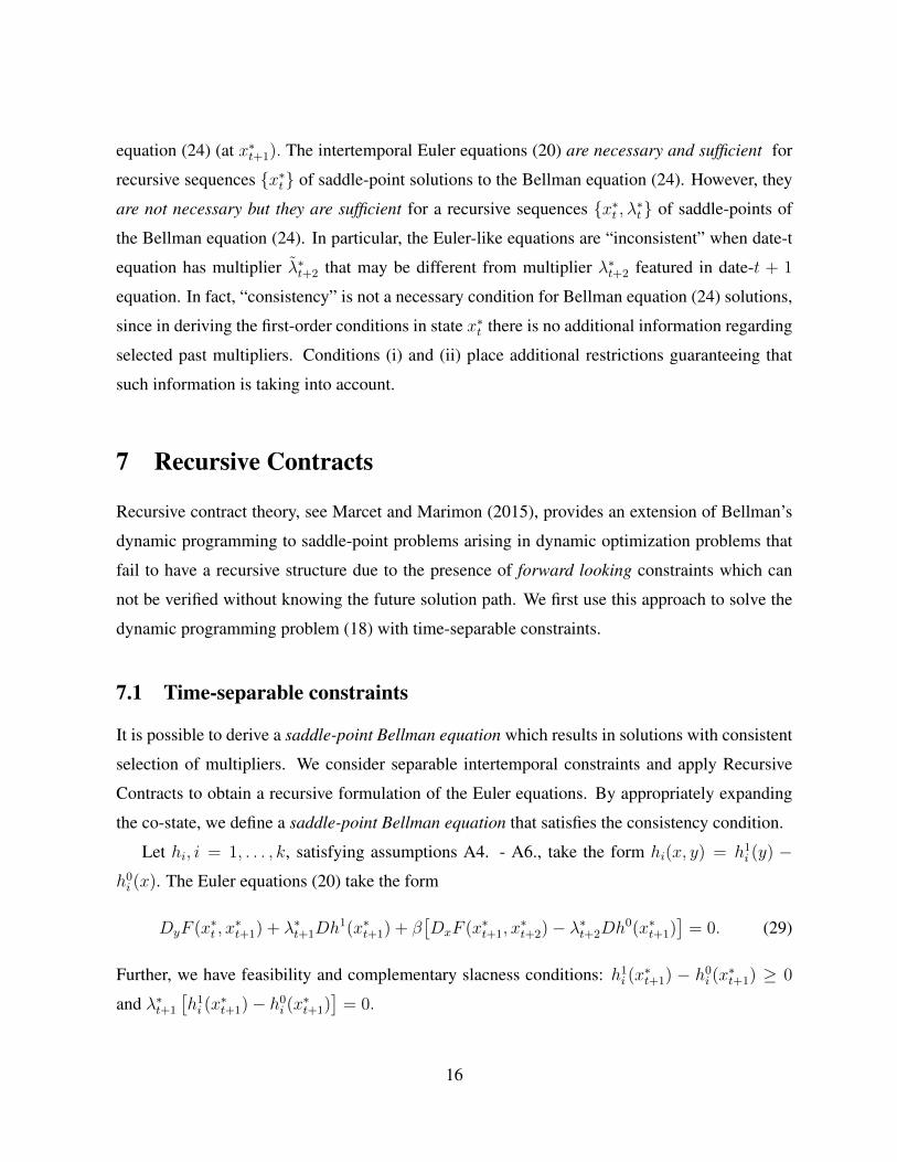
equation (24) (at x∗t+1). The intertemporal Euler equations (20) are necessary and sufficient for

recursive sequences {x∗t} of saddle-point solutions to the Bellman equation (24). However, they

are not necessary but they are sufficient for a recursive sequences {x∗t , λ∗t} of saddle-points of

the Bellman equation (24). In particular, the Euler-like equations are “inconsistent” when date-t

equation has multiplier λ∗t+2 that may be different from multiplier λ∗t+2 featured in date-t + 1

equation. In fact, “consistency” is not a necessary condition for Bellman equation (24) solutions,

since in deriving the first-order conditions in state x∗t there is no additional information regarding

selected past multipliers. Conditions (i) and (ii) place additional restrictions guaranteeing that

such information is taking into account.

7 Recursive Contracts

Recursive contract theory, see Marcet and Marimon (2015), provides an extension of Bellman’s

dynamic programming to saddle-point problems arising in dynamic optimization problems that

fail to have a recursive structure due to the presence of forward looking constraints which can

not be verified without knowing the future solution path. We first use this approach to solve the

dynamic programming problem (18) with time-separable constraints.

7.1 Time-separable constraints

It is possible to derive a saddle-point Bellman equation which results in solutions with consistent

selection of multipliers. We consider separable intertemporal constraints and apply Recursive

Contracts to obtain a recursive formulation of the Euler equations. By appropriately expanding

the co-state, we define a saddle-point Bellman equation that satisfies the consistency condition.

Let hi, i = 1, . . . , k, satisfying assumptions A4. - A6., take the form hi(x, y) = h1i (y) −

h0i (x). The Euler equations (20) take the form

DyF (x∗t , x∗t+1) + λ∗t+1Dh

1(x∗t+1) + β[DxF (x∗t+1, x

∗t+2)− λ∗t+2Dh

0(x∗t+1)]

= 0. (29)

Further, we have feasibility and complementary slacness conditions: h1i (x∗t+1) − h0

i (x∗t+1) ≥ 0

and λ∗t+1

[h1i (x∗t+1)− h0

i (x∗t+1)]

= 0.

16

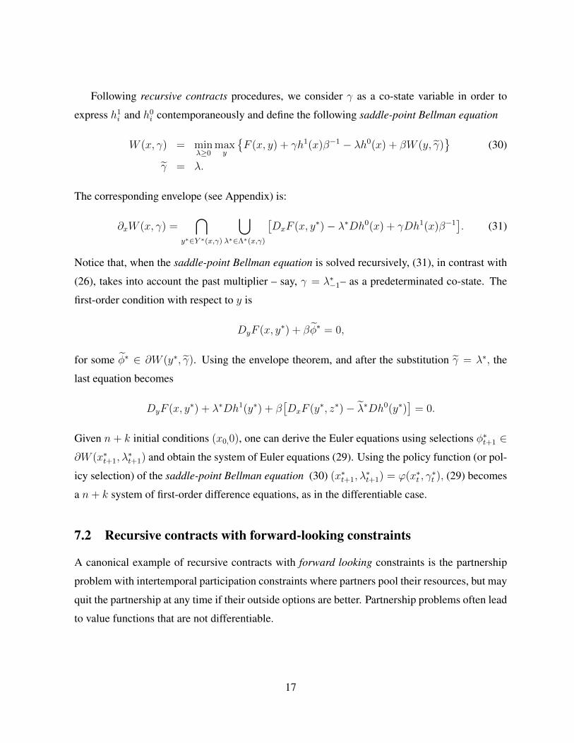
Following recursive contracts procedures, we consider γ as a co-state variable in order to

express h1i and h0

i contemporaneously and define the following saddle-point Bellman equation

W (x, γ) = minλ≥0

maxy

{F (x, y) + γh1(x)β−1 − λh0(x) + βW (y, γ)

}(30)

γ = λ.

The corresponding envelope (see Appendix) is:

∂xW (x, γ) =⋂

y∗∈Y ∗(x,γ)

⋃λ∗∈Λ∗(x,γ)

[DxF (x, y∗)− λ∗Dh0(x) + γDh1(x)β−1

]. (31)

Notice that, when the saddle-point Bellman equation is solved recursively, (31), in contrast with

(26), takes into account the past multiplier – say, γ = λ∗−1– as a predeterminated co-state. The

first-order condition with respect to y is

DyF (x, y∗) + βφ∗ = 0,

for some φ∗ ∈ ∂W (y∗, γ). Using the envelope theorem, and after the substitution γ = λ∗, the

last equation becomes

DyF (x, y∗) + λ∗Dh1(y∗) + β[DxF (y∗, z∗)− λ∗Dh0(y∗)

]= 0.

Given n+ k initial conditions (x0,0), one can derive the Euler equations using selections φ∗t+1 ∈∂W (x∗t+1, λ

∗t+1) and obtain the system of Euler equations (29). Using the policy function (or pol-

icy selection) of the saddle-point Bellman equation (30) (x∗t+1, λ∗t+1) = ϕ(x∗t , γ

∗t ), (29) becomes

a n+ k system of first-order difference equations, as in the differentiable case.

7.2 Recursive contracts with forward-looking constraints

A canonical example of recursive contracts with forward looking constraints is the partnership

problem with intertemporal participation constraints where partners pool their resources, but may

quit the partnership at any time if their outside options are better. Partnership problems often lead

to value functions that are not differentiable.

17

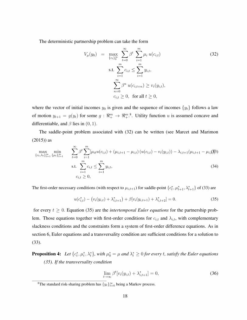
The deterministic partnership problem can take the form

Vµ(y0) = max{ct}∞0

∞∑t=0

βtm∑i=1

µi u(ci,t) (32)

s.t.m∑i=1

ci,t ≤m∑i=1

yi,t,

∞∑n=0

βn u(ci,t+n) ≥ vi(yi,t),

ci,t ≥ 0, for all t ≥ 0,

where the vector of initial incomes y0 is given and the sequence of incomes {yt} follows a law

of motion yt+1 = g(yt) for some g : <m+ → <m+ .8. Utility function u is assumed concave and

differentiable, and β lies in (0, 1).

The saddle-point problem associated with (32) can be written (see Marcet and Marimon

(2015)) as

max{ct,λt}∞t=1

min{µt}∞t=1

∞∑t=0

βtm∑i=1

[µitu(ci,t) + (µi,t+1 − µi,t) (u(ci,t)− vi(yi,t))− λi,t+1(µi,t+1 − µi,t)](33)

s.t.m∑i=1

ci,t ≤m∑i=1

yi,t, (34)

ci,t ≥ 0,

The first-order necessary conditions (with respect to µi,t+1) for saddle-point {c∗t , µ∗t+1, λ∗t+1} of (33) are

u(c∗i,t)−(vi(yi,t) + λ∗i,t+1

)+ β[vi(yi,t+1) + λ∗i,t+2] = 0. (35)

for every t ≥ 0. Equation (35) are the intertemporal Euler equations for the partnership prob-

lem. Those equations together with first-order conditions for ci,t and λi,t, with complementary

slackness conditions and the constraints form a system of first-order difference equations. As in

section 6, Euler equations and a transversality condition are sufficient conditions for a solution to

(33).

Proposition 4: Let {c∗t , µ∗t , λ∗t}, with µ∗0 = µ and λ∗t ≥ 0 for every t, satisfy the Euler equations

(35). If the transversality condition

limt→∞

βt[vi(yi,t) + λ∗i,t+1] = 0, (36)

8The standard risk-sharing problem has {yt}∞t=0 being a Markov process.

18

holds, then {c∗t} is a solution to the partnership problem (32).

Marcet and Marimon (2015) show that the value function Vµ satisfies Vµ(y0) = W (y0, µ),

where function W is the value function of the following saddle-point Bellman equation

W ( y, µ) = minµ

maxc

{ m∑i=1

µiu(ci) + (µi − µi) (u(ci)− vi(yi)) + βW (y, µ)

}(37)

s.t.m∑i=1

ci ≤m∑i=1

yi (38)

µi ≥ µi, (39)

ci ≥ 0, for all i,

where y = g(y). If the function u is concave, then the order of maximum and minimum does not

matter and the common value is the saddle-value. Further, there exists a saddle-point (µ∗, c∗). By

a solution to the saddle-point Bellman equation we always mean a saddle-point.

For every solution {c∗t} to (32), there exists a sequence {µ∗t+1} such that {(c∗t , µ∗t+1)} is a se-

quence of recursive solutions to Bellman equation (37). In contrast to the dynamic programming

problem of Section 6, the converse holds true only under an additional consistency condition of

Marcet and Marimon (2015). We elaborate on this below.

The value function W is convex in µ. The envelope relation for saddle-point problem (69) in

the Appendix implies that the subdifferential of W with respect to µ is

∂µW (y, µ) = v(y) +⋃c∗

Λ∗c∗(k, y, µ) (40)

where the union is taken over all solutions c∗ to (37) and Λ∗c∗(y, µ) denotes the set of saddle-point

multipliers of the constraint (39) corresponding to solution c∗. Function W is differentiable with

respect to µ at (y, µ) if and only if there is unique multiplier λ∗ that is common to all solutions.

Consider a sequence {(µ∗t+1, c∗t , λ∗t+1)} of solutions to the saddle-point Bellman equations

(37). The first-order conditions with respect to µ state that there exists φ∗t+1 ∈ ∂Wµ(yt+1, µ∗t+1)

such that

u(c∗i,t)−(vi(yi,t) + λ∗i,t+1

)+ βφ∗i,t+1 = 0, (41)

where φ∗i,t+1 is the coordinate of subgradient vector φ∗t+1 corresponding to µi. The envelope

representation (40) of ∂Wµ(yt+1, µ∗t+1) implies that there is λ∗t+2 ∈ Λ∗c∗t+1

(yt+1, µ∗t+1) such that

φ∗i,t+1 = vi(yi,t) + λ∗i,t+2 (42)

19

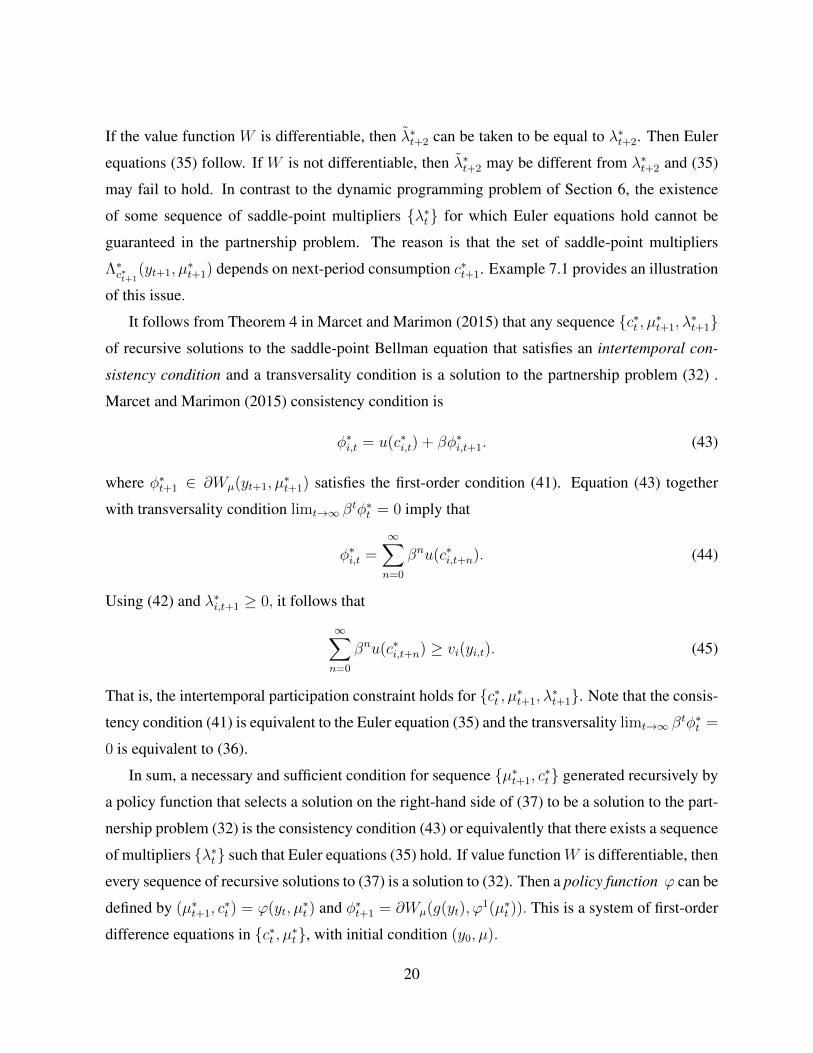
If the value function W is differentiable, then λ∗t+2 can be taken to be equal to λ∗t+2. Then Euler

equations (35) follow. If W is not differentiable, then λ∗t+2 may be different from λ∗t+2 and (35)

may fail to hold. In contrast to the dynamic programming problem of Section 6, the existence

of some sequence of saddle-point multipliers {λ∗t} for which Euler equations hold cannot be

guaranteed in the partnership problem. The reason is that the set of saddle-point multipliers

Λ∗c∗t+1(yt+1, µ

∗t+1) depends on next-period consumption c∗t+1. Example 7.1 provides an illustration

of this issue.

It follows from Theorem 4 in Marcet and Marimon (2015) that any sequence {c∗t , µ∗t+1, λ∗t+1}

of recursive solutions to the saddle-point Bellman equation that satisfies an intertemporal con-

sistency condition and a transversality condition is a solution to the partnership problem (32) .

Marcet and Marimon (2015) consistency condition is

φ∗i,t = u(c∗i,t) + βφ∗i,t+1. (43)

where φ∗t+1 ∈ ∂Wµ(yt+1, µ∗t+1) satisfies the first-order condition (41). Equation (43) together

with transversality condition limt→∞ βtφ∗t = 0 imply that

φ∗i,t =∞∑n=0

βnu(c∗i,t+n). (44)

Using (42) and λ∗i,t+1 ≥ 0, it follows that

∞∑n=0

βnu(c∗i,t+n) ≥ vi(yi,t). (45)

That is, the intertemporal participation constraint holds for {c∗t , µ∗t+1, λ∗t+1}. Note that the consis-

tency condition (41) is equivalent to the Euler equation (35) and the transversality limt→∞ βtφ∗t =

0 is equivalent to (36).

In sum, a necessary and sufficient condition for sequence {µ∗t+1, c∗t} generated recursively by

a policy function that selects a solution on the right-hand side of (37) to be a solution to the part-

nership problem (32) is the consistency condition (43) or equivalently that there exists a sequence

of multipliers {λ∗t} such that Euler equations (35) hold. If value functionW is differentiable, then

every sequence of recursive solutions to (37) is a solution to (32). Then a policy function ϕ can be

defined by (µ∗t+1, c∗t ) = ϕ(yt, µ

∗t ) and φ∗t+1 = ∂Wµ(g(yt), ϕ

1(µ∗t )). This is a system of first-order

difference equations in {c∗t , µ∗t}, with initial condition (y0, µ).

20

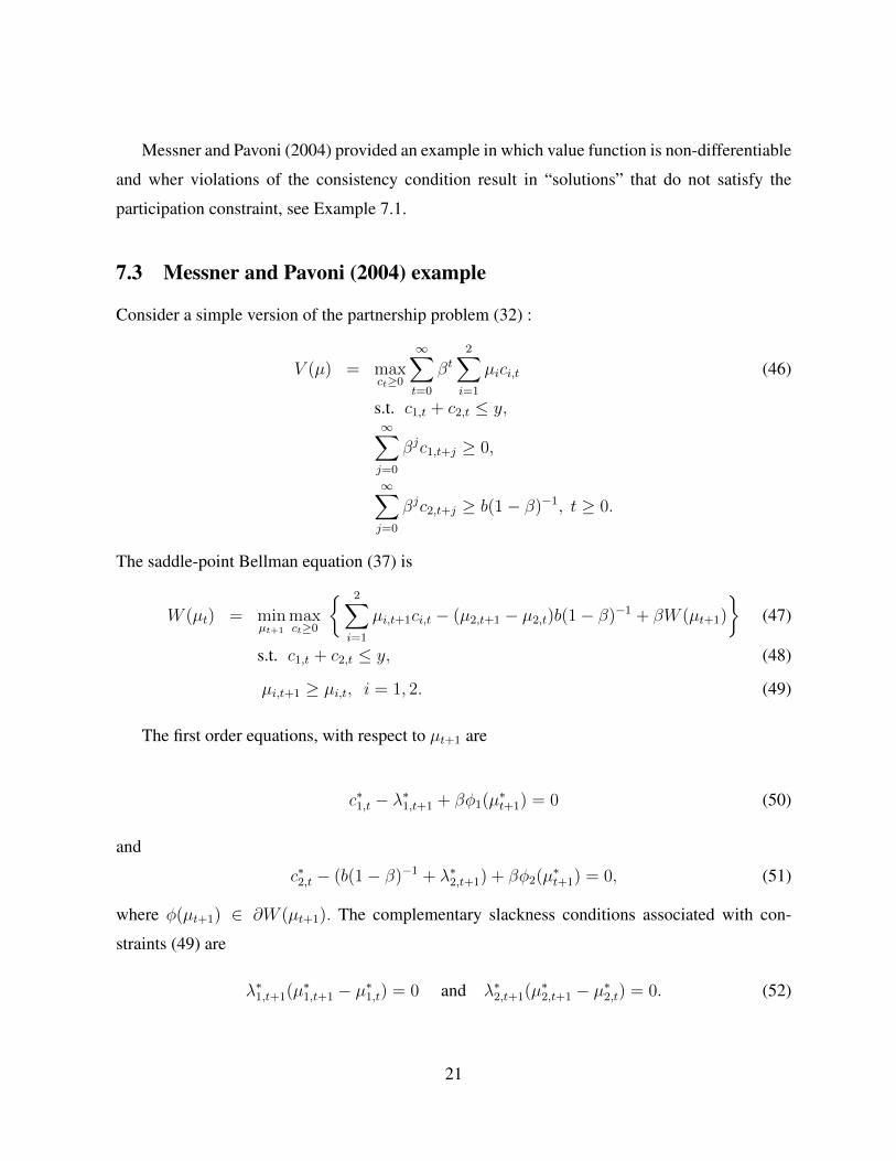
Messner and Pavoni (2004) provided an example in which value function is non-differentiable

and wher violations of the consistency condition result in “solutions” that do not satisfy the

participation constraint, see Example 7.1.

7.3 Messner and Pavoni (2004) example

Consider a simple version of the partnership problem (32) :

V (µ) = maxct≥0

∞∑t=0

βt2∑i=1

µici,t (46)

s.t. c1,t + c2,t ≤ y,∞∑j=0

βjc1,t+j ≥ 0,

∞∑j=0

βjc2,t+j ≥ b(1− β)−1, t ≥ 0.

The saddle-point Bellman equation (37) is

W (µt) = minµt+1

maxct≥0

{ 2∑i=1

µi,t+1ci,t − (µ2,t+1 − µ2,t)b(1− β)−1 + βW (µt+1)

}(47)

s.t. c1,t + c2,t ≤ y, (48)

µi,t+1 ≥ µi,t, i = 1, 2. (49)

The first order equations, with respect to µt+1 are

c∗1,t − λ∗1,t+1 + βφ1(µ∗t+1) = 0 (50)

and

c∗2,t − (b(1− β)−1 + λ∗2,t+1) + βφ2(µ∗t+1) = 0, (51)

where φ(µt+1) ∈ ∂W (µt+1). The complementary slackness conditions associated with con-

straints (49) are

λ∗1,t+1(µ∗1,t+1 − µ∗1,t) = 0 and λ∗2,t+1(µ∗2,t+1 − µ∗2,t) = 0. (52)

21

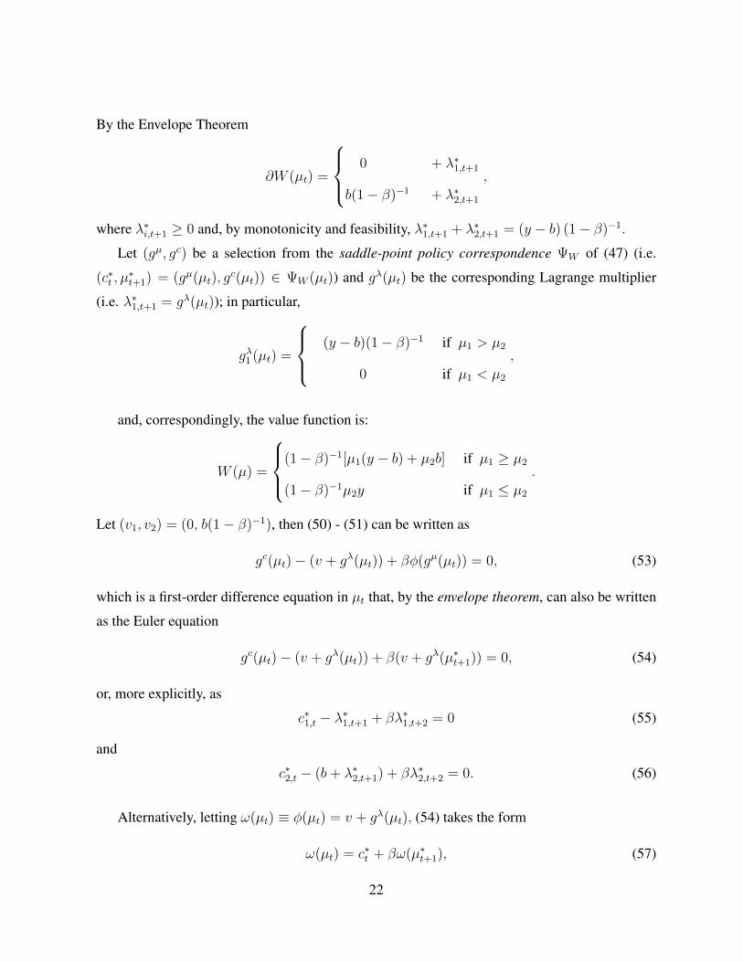
By the Envelope Theorem

∂W (µt) =

0 + λ∗1,t+1

b(1− β)−1 + λ∗2,t+1

,

where λ∗i,t+1 ≥ 0 and, by monotonicity and feasibility, λ∗1,t+1 + λ∗2,t+1 = (y − b) (1− β)−1.

Let (gµ, gc) be a selection from the saddle-point policy correspondence ΨW of (47) (i.e.

(c∗t , µ∗t+1) = (gµ(µt), g

c(µt)) ∈ ΨW (µt)) and gλ(µt) be the corresponding Lagrange multiplier

(i.e. λ∗1,t+1 = gλ(µt)); in particular,

gλ1 (µt) =

(y − b)(1− β)−1 if µ1 > µ2

0 if µ1 < µ2

,

and, correspondingly, the value function is:

W (µ) =

(1− β)−1[µ1(y − b) + µ2b] if µ1 ≥ µ2

(1− β)−1µ2y if µ1 ≤ µ2

.

Let (v1, v2) = (0, b(1− β)−1), then (50) - (51) can be written as

gc(µt)− (v + gλ(µt)) + βφ(gµ(µt)) = 0, (53)

which is a first-order difference equation in µt that, by the envelope theorem, can also be written

as the Euler equation

gc(µt)− (v + gλ(µt)) + β(v + gλ(µ∗t+1)) = 0, (54)

or, more explicitly, as

c∗1,t − λ∗1,t+1 + βλ∗1,t+2 = 0 (55)

and

c∗2,t − (b+ λ∗2,t+1) + βλ∗2,t+2 = 0. (56)

Alternatively, letting ω(µt) ≡ φ(µt) = v + gλ(µt), (54) takes the form

ω(µt) = c∗t + βω(µ∗t+1), (57)

22

showing that the consistency condition in Marcet and Marimon (2015; Theorem 4) is the Eu-

ler equation of (47), with respect to µ. Furthermore, being derived from (54) the transveraslity

condition, limn−→∞ βnω(µ∗t+n) = 0, is redundant. However, there is an implicit intertemporal

consistency condition in the system of Euler equations (57): the solution to (47) at µ∗t+1 is given

by (53) at µ∗t+1, which not only involves the state µ∗t+1 and its change of state, gµ(µ∗t+1), but also

the Lagrange multiplier gλ(µ∗t+1), which already appears in (53) at µ∗t .

Messner and Pavoni did not have at their disposal the envelope theorem, and the correspond-

ing Euler equation, discussed in this paper, and considered the solution of (47) at µ∗t+1 (where

µ∗1,t+1 = µ∗2,t+1) not taking into account that gλ(µ∗t+1) was predetermined by the solution of (47)

at µ∗t . In our formulation, this would correspond to finding an arbitrary solution, such as

c∗t+1 − (v + λ∗t+1) + βφ(µ∗t+2)) = 0,

which would violate (57) at µt, whenever (v + λ∗t+1) 6= ω(µ∗t+1).

More precisely, we can solve (46) from an intial µ1,0 > µ2,0. That is, λ∗2,1 = 0 and, using

complementary slackness (49), we obtain µ∗1,1 = µ1,0, while µ∗2,1 = µ∗1,1. Using (55 ) -(56), we

obtain

c∗1,0 = (y − b)(1− β)−1 − βλ∗1,2 and c∗2,0 = b− βλ∗2,2 (58)

These equations, together with the constraint c∗1,0 +c∗2,0 = y (i.e. λ∗1,2 +λ∗2,2 = (y − b) (1−β)−1),

determine c∗1,0, c∗2,0, given λ∗2,2 ∈ [0, (y − b) (1− β)−1] . In other words, there is an indeterminacy

of period zero solutions parametrized by λ∗2,2. As we have seen, making a selection gλ(gµ(µ0))

resolves this indeterminacy, but also determines λ∗2 in the first-order conditions (53) at µ∗1.

In sum, we have shown that using the appropriate envelope theorem and Euler equations the

saddle-point Bellman equation generates the correct solution to Messner and Pavoni (2004) ex-

ample. Nevertheless, this example shows the differences between the saddle-point dynamic pro-

gramming without differentiability and standard dynamic programming, and with saddle-point

dynamic programming with differentiability (e.g. with unique solutions). In standard dynamic

programming, if there are multiple solutions between two states – say, x∗t and x∗t+1 – all the se-

lections from the policy correspondence have the same value. With forward-looking constraints

this is also true for the aggregate value function W , but not for the individual value functions

ωi. Nevertheless, if W is differentiable there is no selection to be made and, therefore, the Euler

23

equation (57) at µ∗t+1 does not depend on gλ(µ∗t ).

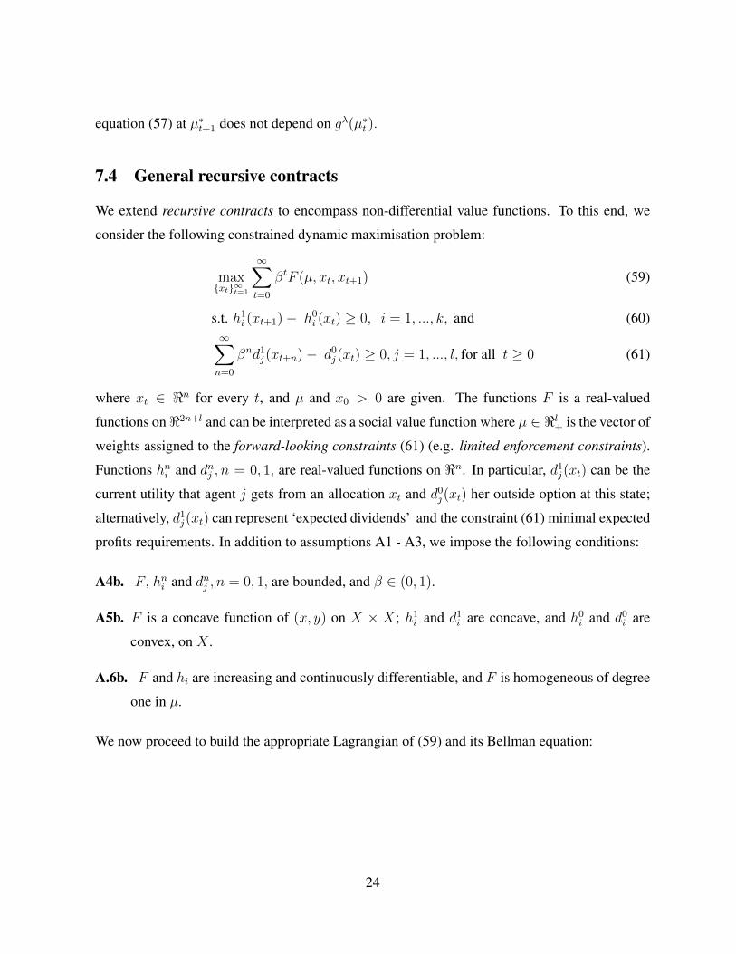
7.4 General recursive contracts

We extend recursive contracts to encompass non-differential value functions. To this end, we

consider the following constrained dynamic maximisation problem:

max{xt}∞t=1

∞∑t=0

βtF (µ, xt, xt+1) (59)

s.t. h1i (xt+1)− h0

i (xt) ≥ 0, i = 1, ..., k, and (60)∞∑n=0

βnd1j(xt+n)− d0

j(xt) ≥ 0, j = 1, ..., l, for all t ≥ 0 (61)

where xt ∈ <n for every t, and µ and x0 > 0 are given. The functions F is a real-valued

functions on<2n+l and can be interpreted as a social value function where µ ∈ <l+ is the vector of

weights assigned to the forward-looking constraints (61) (e.g. limited enforcement constraints).

Functions hni and dnj , n = 0, 1, are real-valued functions on <n. In particular, d1j(xt) can be the

current utility that agent j gets from an allocation xt and d0j(xt) her outside option at this state;

alternatively, d1j(xt) can represent ‘expected dividends’ and the constraint (61) minimal expected

profits requirements. In addition to assumptions A1 - A3, we impose the following conditions:

A4b. F , hni and dnj , n = 0, 1, are bounded, and β ∈ (0, 1).

A5b. F is a concave function of (x, y) on X × X; h1i and d1

i are concave, and h0i and d0

i are

convex, on X .

A.6b. F and hi are increasing and continuously differentiable, and F is homogeneous of degree

one in µ.

We now proceed to build the appropriate Lagrangian of (59) and its Bellman equation:

24

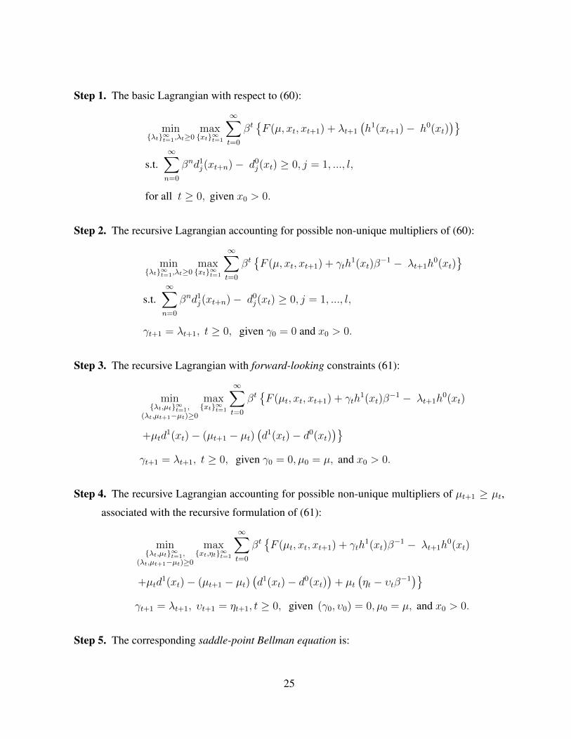
Step 1. The basic Lagrangian with respect to (60):

min{λt}∞t=1,λt≥0

max{xt}∞t=1

∞∑t=0

βt{F (µ, xt, xt+1) + λt+1

(h1(xt+1)− h0(xt)

)}s.t.

∞∑n=0

βnd1j(xt+n)− d0

j(xt) ≥ 0, j = 1, ..., l,

for all t ≥ 0, given x0 > 0.

Step 2. The recursive Lagrangian accounting for possible non-unique multipliers of (60):

min{λt}∞t=1,λt≥0

max{xt}∞t=1

∞∑t=0

βt{F (µ, xt, xt+1) + γth

1(xt)β−1 − λt+1h

0(xt)}

s.t.∞∑n=0

βnd1j(xt+n)− d0

j(xt) ≥ 0, j = 1, ..., l,

γt+1 = λt+1, t ≥ 0, given γ0 = 0 and x0 > 0.

Step 3. The recursive Lagrangian with forward-looking constraints (61):

min{λt,µt}∞t=1,

(λt,µt+1−µt)≥0

max{xt}∞t=1

∞∑t=0

βt{F (µt, xt, xt+1) + γth

1(xt)β−1 − λt+1h

0(xt)

+µtd1(xt)− (µt+1 − µt)

(d1(xt)− d0(xt)

)}γt+1 = λt+1, t ≥ 0, given γ0 = 0, µ0 = µ, and x0 > 0.

Step 4. The recursive Lagrangian accounting for possible non-unique multipliers of µt+1 ≥ µt,

associated with the recursive formulation of (61):

min{λt,µt}∞t=1,

(λt,µt+1−µt)≥0

max{xt,ηt}∞t=1

∞∑t=0

βt{F (µt, xt, xt+1) + γth

1(xt)β−1 − λt+1h

0(xt)

+µtd1(xt)− (µt+1 − µt)

(d1(xt)− d0(xt)

)+ µt

(ηt − υtβ−1

)}γt+1 = λt+1, υt+1 = ηt+1, t ≥ 0, given (γ0, υ0) = 0, µ0 = µ, and x0 > 0.

Step 5. The corresponding saddle-point Bellman equation is:

25

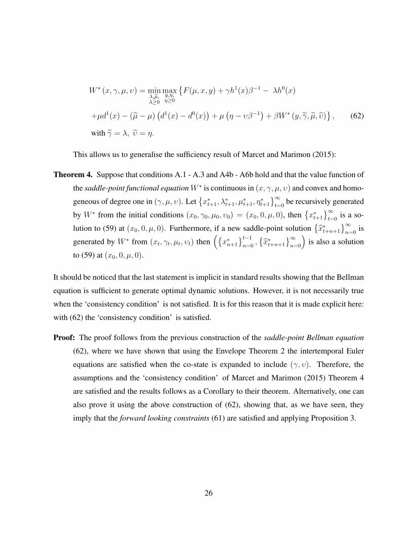
W ∗ (x, γ, µ, υ) = minλ,µ,λ≥0

maxy,η,η≥0

{F (µ, x, y) + γh1(x)β−1 − λh0(x)

+µd1(x)− (µ− µ)(d1(x)− d0(x)

)+ µ

(η − υβ−1

)+ βW ∗ (y, γ, µ, υ)

}, (62)

with γ = λ, υ = η.

This allows us to generalise the sufficiency result of Marcet and Marimon (2015):

Theorem 4. Suppose that conditions A.1 - A.3 and A4b - A6b hold and that the value function of

the saddle-point functional equationW ∗ is continuous in (x, γ, µ, υ) and convex and homo-

geneous of degree one in (γ, µ, υ). Let{x∗t+1, λ

∗t+1, µ

∗t+1, η

∗t+1

}∞t=0

be recursively generated

by W ∗ from the initial conditions (x0, γ0, µ0, υ0) = (x0, 0, µ, 0), then{x∗t+1

}∞t=0

is a so-

lution to (59) at (x0, 0, µ, 0). Furthermore, if a new saddle-point solution{x∗t+n+1

}∞n=0

is

generated by W ∗ from (xt, γt, µt, υt) then({x∗n+1

}t−1

n=0,{x∗t+n+1

}∞n=0

)is also a solution

to (59) at (x0, 0, µ, 0).

It should be noticed that the last statement is implicit in standard results showing that the Bellman

equation is sufficient to generate optimal dynamic solutions. However, it is not necessarily true

when the ‘consistency condition’ is not satisfied. It is for this reason that it is made explicit here:

with (62) the ‘consistency condition’ is satisfied.

Proof: The proof follows from the previous construction of the saddle-point Bellman equation

(62), where we have shown that using the Envelope Theorem 2 the intertemporal Euler

equations are satisfied when the co-state is expanded to include (γ, υ). Therefore, the

assumptions and the ‘consistency condition’ of Marcet and Marimon (2015) Theorem 4

are satisfied and the results follows as a Corollary to their theorem. Alternatively, one can

also prove it using the above construction of (62), showing that, as we have seen, they

imply that the forward looking constraints (61) are satisfied and applying Proposition 3.

26

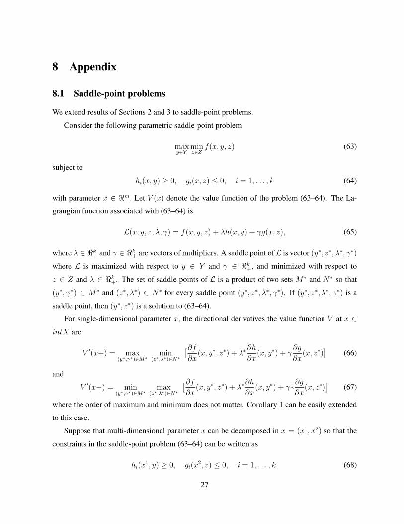
8 Appendix

8.1 Saddle-point problems

We extend results of Sections 2 and 3 to saddle-point problems.

Consider the following parametric saddle-point problem

maxy∈Y

minz∈Z

f(x, y, z) (63)

subject to

hi(x, y) ≥ 0, gi(x, z) ≤ 0, i = 1, . . . , k (64)

with parameter x ∈ <m. Let V (x) denote the value function of the problem (63–64). The La-

grangian function associated with (63–64) is

L(x, y, z, λ, γ) = f(x, y, z) + λh(x, y) + γg(x, z), (65)

where λ ∈ <k+ and γ ∈ <k+ are vectors of multipliers. A saddle point ofL is vector (y∗, z∗, λ∗, γ∗)

where L is maximized with respect to y ∈ Y and γ ∈ <k+, and minimized with respect to

z ∈ Z and λ ∈ <k+. The set of saddle points of L is a product of two sets M∗ and N∗ so that

(y∗, γ∗) ∈ M∗ and (z∗, λ∗) ∈ N∗ for every saddle point (y∗, z∗, λ∗, γ∗). If (y∗, z∗, λ∗, γ∗) is a

saddle point, then (y∗, z∗) is a solution to (63–64).

For single-dimensional parameter x, the directional derivatives the value function V at x ∈intX are

V ′(x+) = max(y∗,γ∗)∈M∗

min(z∗,λ∗)∈N∗

[∂f∂x

(x, y∗, z∗) + λ∗∂h

∂x(x, y∗) + γ

∂g

∂x(x, z∗)

](66)

and

V ′(x−) = min(y∗,γ∗)∈M∗

max(z∗,λ∗)∈N∗

[∂f∂x

(x, y∗, z∗) + λ∗∂h

∂x(x, y∗) + γ∗∂g

∂x(x, z∗)

](67)

where the order of maximum and minimum does not matter. Corollary 1 can be easily extended

to this case.

Suppose that multi-dimensional parameter x can be decomposed in x = (x1, x2) so that the

constraints in the saddle-point problem (63–64) can be written as

hi(x1, y) ≥ 0, gi(x

2, z) ≤ 0, i = 1, . . . , k. (68)

27

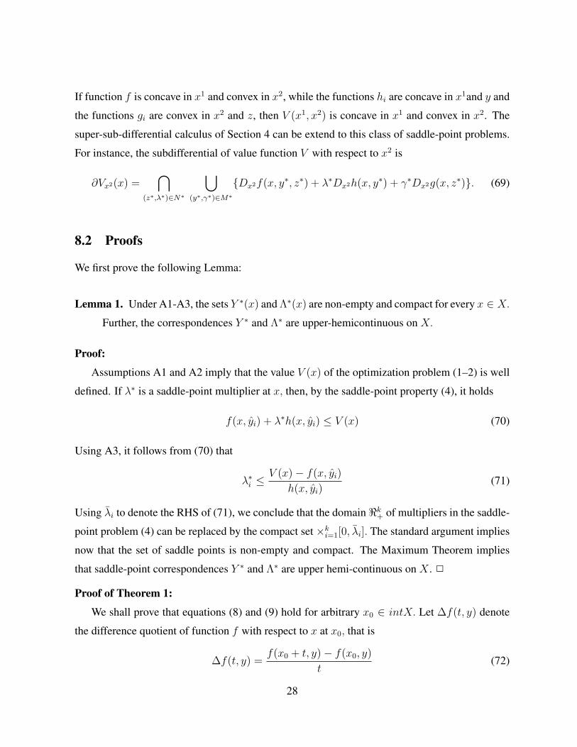
If function f is concave in x1 and convex in x2, while the functions hi are concave in x1and y and

the functions gi are convex in x2 and z, then V (x1, x2) is concave in x1 and convex in x2. The

super-sub-differential calculus of Section 4 can be extend to this class of saddle-point problems.

For instance, the subdifferential of value function V with respect to x2 is

∂Vx2(x) =⋂

(z∗,λ∗)∈N∗

⋃(y∗,γ∗)∈M∗

{Dx2f(x, y∗, z∗) + λ∗Dx2h(x, y∗) + γ∗Dx2g(x, z∗)}. (69)

8.2 Proofs

We first prove the following Lemma:

Lemma 1. Under A1-A3, the sets Y ∗(x) and Λ∗(x) are non-empty and compact for every x ∈ X.Further, the correspondences Y ∗ and Λ∗ are upper-hemicontinuous on X.

Proof:

Assumptions A1 and A2 imply that the value V (x) of the optimization problem (1–2) is well

defined. If λ∗ is a saddle-point multiplier at x, then, by the saddle-point property (4), it holds

f(x, yi) + λ∗h(x, yi) ≤ V (x) (70)

Using A3, it follows from (70) that

λ∗i ≤V (x)− f(x, yi)

h(x, yi)(71)

Using λi to denote the RHS of (71), we conclude that the domain <k+ of multipliers in the saddle-

point problem (4) can be replaced by the compact set ×ki=1[0, λi]. The standard argument implies

now that the set of saddle points is non-empty and compact. The Maximum Theorem implies

that saddle-point correspondences Y ∗ and Λ∗ are upper hemi-continuous on X . 2

Proof of Theorem 1:

We shall prove that equations (8) and (9) hold for arbitrary x0 ∈ intX. Let ∆f(t, y) denote

the difference quotient of function f with respect to x at x0, that is

∆f(t, y) =f(x0 + t, y)− f(x0, y)

t(72)

28

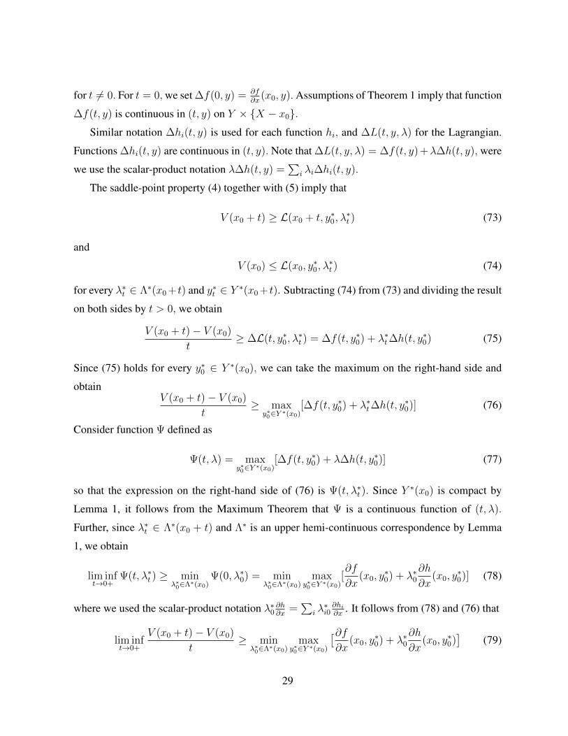
for t 6= 0. For t = 0,we set ∆f(0, y) = ∂f∂x

(x0, y).Assumptions of Theorem 1 imply that function

∆f(t, y) is continuous in (t, y) on Y × {X − x0}.Similar notation ∆hi(t, y) is used for each function hi, and ∆L(t, y, λ) for the Lagrangian.

Functions ∆hi(t, y) are continuous in (t, y). Note that ∆L(t, y, λ) = ∆f(t, y) +λ∆h(t, y), were

we use the scalar-product notation λ∆h(t, y) =∑

i λi∆hi(t, y).

The saddle-point property (4) together with (5) imply that

V (x0 + t) ≥ L(x0 + t, y∗0, λ∗t ) (73)

and

V (x0) ≤ L(x0, y∗0, λ

∗t ) (74)

for every λ∗t ∈ Λ∗(x0 + t) and y∗t ∈ Y ∗(x0 + t). Subtracting (74) from (73) and dividing the result

on both sides by t > 0, we obtain

V (x0 + t)− V (x0)

t≥ ∆L(t, y∗0, λ

∗t ) = ∆f(t, y∗0) + λ∗t∆h(t, y∗0) (75)

Since (75) holds for every y∗0 ∈ Y ∗(x0), we can take the maximum on the right-hand side and

obtainV (x0 + t)− V (x0)

t≥ max

y∗0∈Y ∗(x0)[∆f(t, y∗0) + λ∗t∆h(t, y∗0)] (76)

Consider function Ψ defined as

Ψ(t, λ) = maxy∗0∈Y ∗(x0)

[∆f(t, y∗0) + λ∆h(t, y∗0)] (77)

so that the expression on the right-hand side of (76) is Ψ(t, λ∗t ). Since Y ∗(x0) is compact by

Lemma 1, it follows from the Maximum Theorem that Ψ is a continuous function of (t, λ).

Further, since λ∗t ∈ Λ∗(x0 + t) and Λ∗ is an upper hemi-continuous correspondence by Lemma

1, we obtain

lim inft→0+

Ψ(t, λ∗t ) ≥ minλ∗0∈Λ∗(x0)

Ψ(0, λ∗0) = minλ∗0∈Λ∗(x0)

maxy∗0∈Y ∗(x0)

[∂f

∂x(x0, y

∗0) + λ∗0

∂h

∂x(x0, y

∗0)] (78)

where we used the scalar-product notation λ∗0∂h∂x

=∑

i λ∗i0∂hi∂x

. It follows from (78) and (76) that

lim inft→0+

V (x0 + t)− V (x0)

t≥ min

λ∗0∈Λ∗(x0)max

y∗0∈Y ∗(x0)

[∂f∂x

(x0, y∗0) + λ∗0

∂h

∂x(x0, y

∗0)]

(79)

29

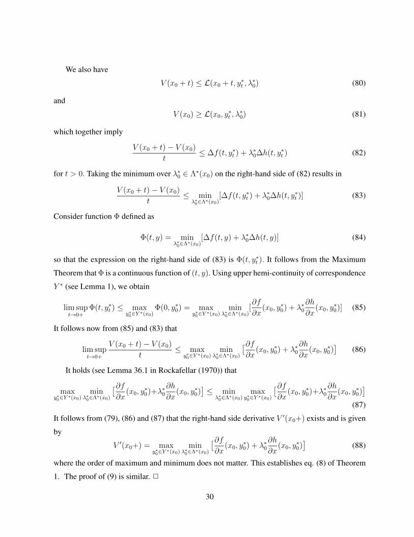
We also have

V (x0 + t) ≤ L(x0 + t, y∗t , λ∗0) (80)

and

V (x0) ≥ L(x0, y∗t , λ

∗0) (81)

which together imply

V (x0 + t)− V (x0)

t≤ ∆f(t, y∗t ) + λ∗0∆h(t, y∗t ) (82)

for t > 0. Taking the minimum over λ∗0 ∈ Λ∗(x0) on the right-hand side of (82) results in

V (x0 + t)− V (x0)

t≤ min

λ∗0∈Λ∗(x0)[∆f(t, y∗t ) + λ∗0∆h(t, y∗t )] (83)

Consider function Φ defined as

Φ(t, y) = minλ∗0∈Λ∗(x0)

[∆f(t, y) + λ∗0∆h(t, y)] (84)

so that the expression on the right-hand side of (83) is Φ(t, y∗t ). It follows from the Maximum

Theorem that Φ is a continuous function of (t, y).Using upper hemi-continuity of correspondence

Y ∗ (see Lemma 1), we obtain

lim supt→0+

Φ(t, y∗t ) ≤ maxy∗0∈Y ∗(x0)

Φ(0, y∗0) = maxy∗0∈Y ∗(x0)

minλ∗0∈Λ∗(x0)

[∂f

∂x(x0, y

∗0) + λ∗0

∂h

∂x(x0, y

∗0)] (85)

It follows now from (85) and (83) that

lim supt→0+

V (x0 + t)− V (x0)

t≤ max

y∗0∈Y ∗(x0)min

λ∗0∈Λ∗(x0)

[∂f∂x

(x0, y∗0) + λ∗0

∂h

∂x(x0, y

∗0)]

(86)

It holds (see Lemma 36.1 in Rockafellar (1970)) that

maxy∗0∈Y ∗(x0)

minλ∗0∈Λ∗(x0)

[∂f∂x

(x0, y∗0)+λ∗0

∂h

∂x(x0, y

∗0)]≤ min

λ∗0∈Λ∗(x0)max

y∗0∈Y ∗(x0)

[∂f∂x

(x0, y∗0)+λ∗0

∂h

∂x(x0, y

∗0)]

(87)

It follows from (79), (86) and (87) that the right-hand side derivative V ′(x0+) exists and is given

by

V ′(x0+) = maxy∗0∈Y ∗(x0)

minλ∗0∈Λ∗(x0)

[∂f∂x

(x0, y∗0) + λ∗0

∂h

∂x(x0, y

∗0)]

(88)

where the order of maximum and minimum does not matter. This establishes eq. (8) of Theorem

1. The proof of (9) is similar. 2

30

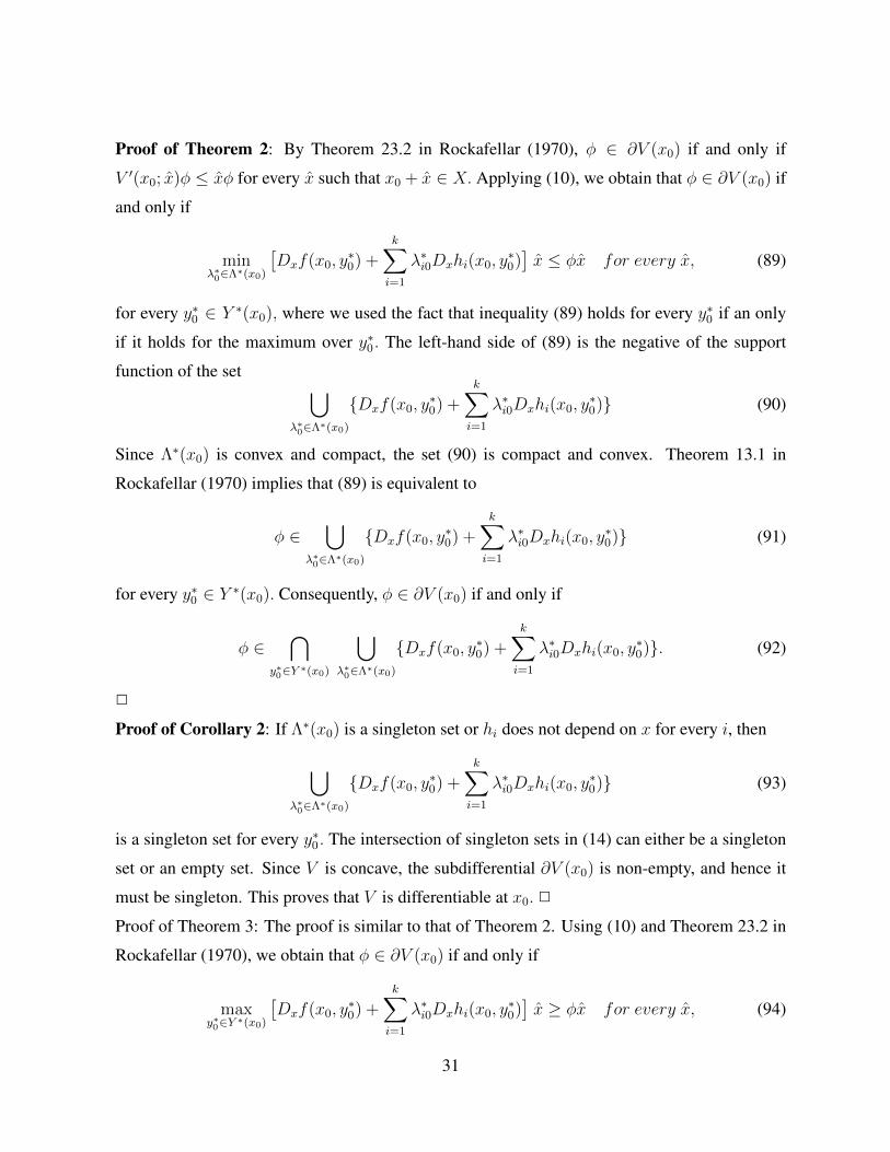
Proof of Theorem 2: By Theorem 23.2 in Rockafellar (1970), φ ∈ ∂V (x0) if and only if

V ′(x0; x)φ ≤ xφ for every x such that x0 + x ∈ X. Applying (10), we obtain that φ ∈ ∂V (x0) if

and only if

minλ∗0∈Λ∗(x0)

[Dxf(x0, y

∗0) +

k∑i=1

λ∗i0Dxhi(x0, y∗0)]x ≤ φx for every x, (89)

for every y∗0 ∈ Y ∗(x0), where we used the fact that inequality (89) holds for every y∗0 if an only

if it holds for the maximum over y∗0. The left-hand side of (89) is the negative of the support

function of the set ⋃λ∗0∈Λ∗(x0)

{Dxf(x0, y∗0) +

k∑i=1

λ∗i0Dxhi(x0, y∗0)} (90)

Since Λ∗(x0) is convex and compact, the set (90) is compact and convex. Theorem 13.1 in

Rockafellar (1970) implies that (89) is equivalent to

φ ∈⋃

λ∗0∈Λ∗(x0)

{Dxf(x0, y∗0) +

k∑i=1

λ∗i0Dxhi(x0, y∗0)} (91)

for every y∗0 ∈ Y ∗(x0). Consequently, φ ∈ ∂V (x0) if and only if

φ ∈⋂

y∗0∈Y ∗(x0)

⋃λ∗0∈Λ∗(x0)

{Dxf(x0, y∗0) +

k∑i=1

λ∗i0Dxhi(x0, y∗0)}. (92)

2

Proof of Corollary 2: If Λ∗(x0) is a singleton set or hi does not depend on x for every i, then

⋃λ∗0∈Λ∗(x0)

{Dxf(x0, y∗0) +

k∑i=1

λ∗i0Dxhi(x0, y∗0)} (93)

is a singleton set for every y∗0. The intersection of singleton sets in (14) can either be a singleton

set or an empty set. Since V is concave, the subdifferential ∂V (x0) is non-empty, and hence it

must be singleton. This proves that V is differentiable at x0. 2

Proof of Theorem 3: The proof is similar to that of Theorem 2. Using (10) and Theorem 23.2 in

Rockafellar (1970), we obtain that φ ∈ ∂V (x0) if and only if

maxy∗0∈Y ∗(x0)

[Dxf(x0, y

∗0) +

k∑i=1

λ∗i0Dxhi(x0, y∗0)]x ≥ φx for every x, (94)

31

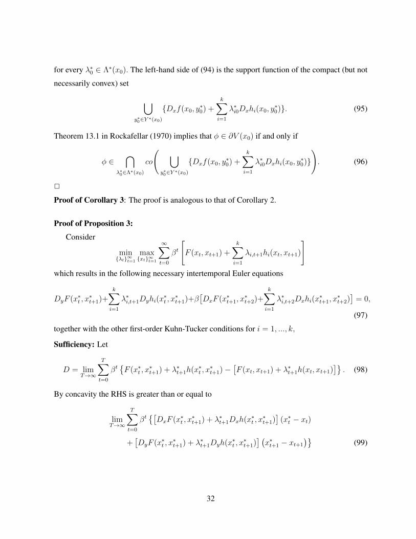
for every λ∗0 ∈ Λ∗(x0). The left-hand side of (94) is the support function of the compact (but not

necessarily convex) set

⋃y∗0∈Y ∗(x0)

{Dxf(x0, y∗0) +

k∑i=1

λ∗i0Dxhi(x0, y∗0)}. (95)

Theorem 13.1 in Rockafellar (1970) implies that φ ∈ ∂V (x0) if and only if

φ ∈⋂

λ∗0∈Λ∗(x0)

co

( ⋃y∗0∈Y ∗(x0)

{Dxf(x0, y∗0) +

k∑i=1

λ∗i0Dxhi(x0, y∗0)}

). (96)

2

Proof of Corollary 3: The proof is analogous to that of Corollary 2.

Proof of Proposition 3:

Consider

min{λt}∞t=1

max{xt}∞t=1

∞∑t=0

βt

[F (xt, xt+1) +

k∑i=1

λi,t+1hi(xt, xt+1)

]which results in the following necessary intertemporal Euler equations

DyF (x∗t , x∗t+1)+

k∑i=1

λ∗i,t+1Dyhi(x∗t , x∗t+1)+β

[DxF (x∗t+1, x

∗t+2)+

k∑i=1

λ∗i,t+2Dxhi(x∗t+1, x

∗t+2)]

= 0,

(97)

together with the other first-order Kuhn-Tucker conditions for i = 1, ..., k,

Sufficiency: Let

D = limT→∞

T∑t=0

βt{F (x∗t , x

∗t+1) + λ∗t+1h(x∗t , x

∗t+1)−

[F (xt, xt+1) + λ∗t+1h(xt, xt+1)

]}. (98)

By concavity the RHS is greater than or equal to

limT→∞

T∑t=0

βt{[DxF (x∗t , x

∗t+1) + λ∗t+1Dxh(x∗t , x

∗t+1)]

(x∗t − xt)

+[DyF (x∗t , x

∗t+1) + λ∗t+1Dyh(x∗t , x

∗t+1)] (x∗t+1 − xt+1

)}(99)

32

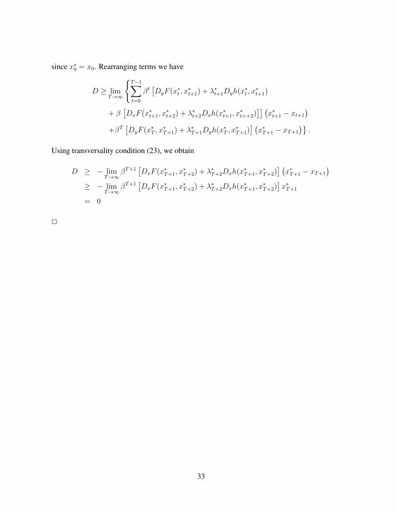
since x∗0 = x0. Rearranging terms we have

D ≥ limT→∞

{T−1∑t=0

βt[DyF (x∗t , x

∗t+1) + λ∗t+1Dyh(x∗t , x

∗t+1)

+ β[DxF (x∗t+1, x

∗t+2) + λ∗t+2Dxh(x∗t+1, x

∗t++2)

]] (x∗t+1 − xt+1

)+βT

[DyF (x∗T , x

∗T+1) + λ∗T+1Dyh(x∗T , x

∗T+1)

] (x∗T+1 − xT+1

)}.

Using transversality condition (23), we obtain

D ≥ − limT→∞

βT+1[DxF (x∗T+1, x

∗T+2) + λ∗T+2Dxh(x∗T+1, x

∗T+2)

] (x∗T+1 − xT+1

)≥ − lim

T→∞βT+1

[DxF (x∗T+1, x

∗T+2) + λ∗T+2Dxh(x∗T+1, x

∗T+2)

]x∗T+1

= 0

2

33

References

L. Benveniste and J. Scheinkman (1979), “Differentiability of the Value Function in Dynamic

Models of Economics” Econometrica, 47, 727–732.

J.-M. Bonnisseau and C. Le Van (1996), “On the Subdifferential of the Value Function in Eco-

nomic Optimization Problems,” Journal of Mathematical Economics, 25, 55–75.

A. Clausen and C. Straub (2011), “Envelope Theorems for Non-Smooth and Non-Concave Opti-

mization,” mimeo.

H. Cole and F. Kubler (2012): “Recursive Contracts, Lotteries and Weakly Concave Pareto Sets”

Review of Economic Dynamics 15(4), 475-500.

T. Kim (1993), “Differentiability of the Value Function,” Seul Journal of Economics, 6, 257–265.

J. Kyparisis (1985), “On Uniqueness of Kuhn-Tucker Multipliers in Nonlinear Programming,”

Mathematical Programming, 32, 242–246.

A. Marcet and R. Marimon (2012), ”Recursive Contracts,” EUI; first version EUI-ECO 1998 #

37 WP.

P. Milgrom and I. Segal (2002), “Envelope Theorems for Arbitrary Choice Sets” Econometrica,

70, 583–601.

M. Messner and N. Pavoni (2004), “On the Recursive Saddle Point Method,” IGIER Working

paper 255, Universita Bocconi.

O. Morand, K. Reffett and S. Tarafdar (2011), “A Nonsmooth Approach to Envelope Theorems,”

mimeo.

J. P. Rincon-Zapatero and M. Santos (2009), “Differentiability of the Value Function without

Interiority Assumptions.” Journal of Economic Theory, 144, 1948-1964.

R.T. Rockafellar. Convex analysis. Princeton University Press, 1970.

R.T. Rockafellar, The Theory of Subgradients and its Applications to Problems of Optimization.

Convex and Nonconvex Functions. Heldermann Verlag, Berlin, 1981.

N.L. Stokey, R. E. Lucas and E. C. Prescott (1989), Recursive Methods in Economic Dynamics.

Cambridge, Ma.: Harvard University Press.

34