The Distribution of Taxes and Government Benefits … Centre for Social and Economic Modelling • University of Canberra • The Distribution of Taxes and Government Benefits in Australia

National Centre for Social and Economic Modelling • University of Canberra •

The Distribution of Taxes and Government Benefits in Australia

Ann Harding, Rachel Lloyd and Neil Warren

Paper presented at the Conference on the Distributional Effects of Government Spending and Taxation, The Levy Economics Institute, 15 October

2004

About NATSEM

The National Centre for Social and Economic Modelling was established on 1 January 1993, and supports its activities through research grants, commissioned research and longer term contracts

for model maintenance and development with the federal departments of Family and Community Services, and

Education, Science and Training.

NATSEM aims to be a key contributor to social and economic policy debate and analysis by developing models of the highest quality, undertaking independent and impartial research, and

supplying valued consultancy services.

Policy changes often have to be made without sufficient information about either the current environment or the

consequences of change. NATSEM specialises in analysing data and producing models so that decision makers have the best

possible quantitative information on which to base their decisions.

NATSEM has an international reputation as a centre of excellence for analysing microdata and constructing microsimulation

models. Such data and models commence with the records of real (but unidentifiable) Australians. Analysis typically begins by looking at either the characteristics or the impact of a policy

change on an individual household, building up to the bigger picture by looking at many individual cases through the use of

large datasets.

It must be emphasised that NATSEM does not have views on policy. All opinions are the authors’ own and are not necessarily

shared by NATSEM.

Director: Ann Harding

© NATSEM, University of Canberra 2004

National Centre for Social and Economic Modelling University of Canberra ACT 2601 Australia

170 Haydon Drive Bruce ACT 2617

Phone + 61 2 6201 2750 Fax + 61 2 6201 2751 Email [email protected] Website www.natsem.canberra.edu.au

v

Abstract

This study examines the distribution of household income, and of selected taxes and benefits in Australia, in 2001-02. We find that direct cash transfers are more progressive than indirect (non-cash) benefits, but that the combined overall impact of all benefits remains strongly redistributive towards lower income Australians. Similarly, the regressive impact of the indirect taxes considered in our study partially offsets the highly progressive impact of direct taxes but the overall impact of the taxes considered remains strongly pro-poor.

Author note

Ann Harding is Professor of Applied Economics and Social Policy, University of Canberra, and Director of the University’s National Centre for Social and Economic Modelling (NATSEM). Rachel Lloyd is a Principal Research Fellow with NATSEM. Professor Neil Warren is Associate Director (Research), Australian Taxation Studies Program at the University of NSW.

Acknowledgments

The authors would like to gratefully acknowledge the input provided to this project by other NATSEM staff, particularly Richard Percival, Annie Abello, Elizabeth Taylor, Ben Phillips, Anthea Bill, Rebecca Cassells and Carol Farbotko. We would also like to acknowledge the hard work of those who build and maintain the STINMOD model, particularly Gillian Beer and Matthew Toohey.

General caveat

NATSEM research findings are generally based on estimated characteristics of the population. Such estimates are usually derived from the application of microsimulation modelling techniques to microdata based on sample surveys. These estimates may be different from the actual characteristics of the population because of sampling and nonsampling errors in the microdata and because of the assumptions underlying the modelling techniques. The microdata do not contain any information that enables identification of the individuals or families to which they refer.

vi

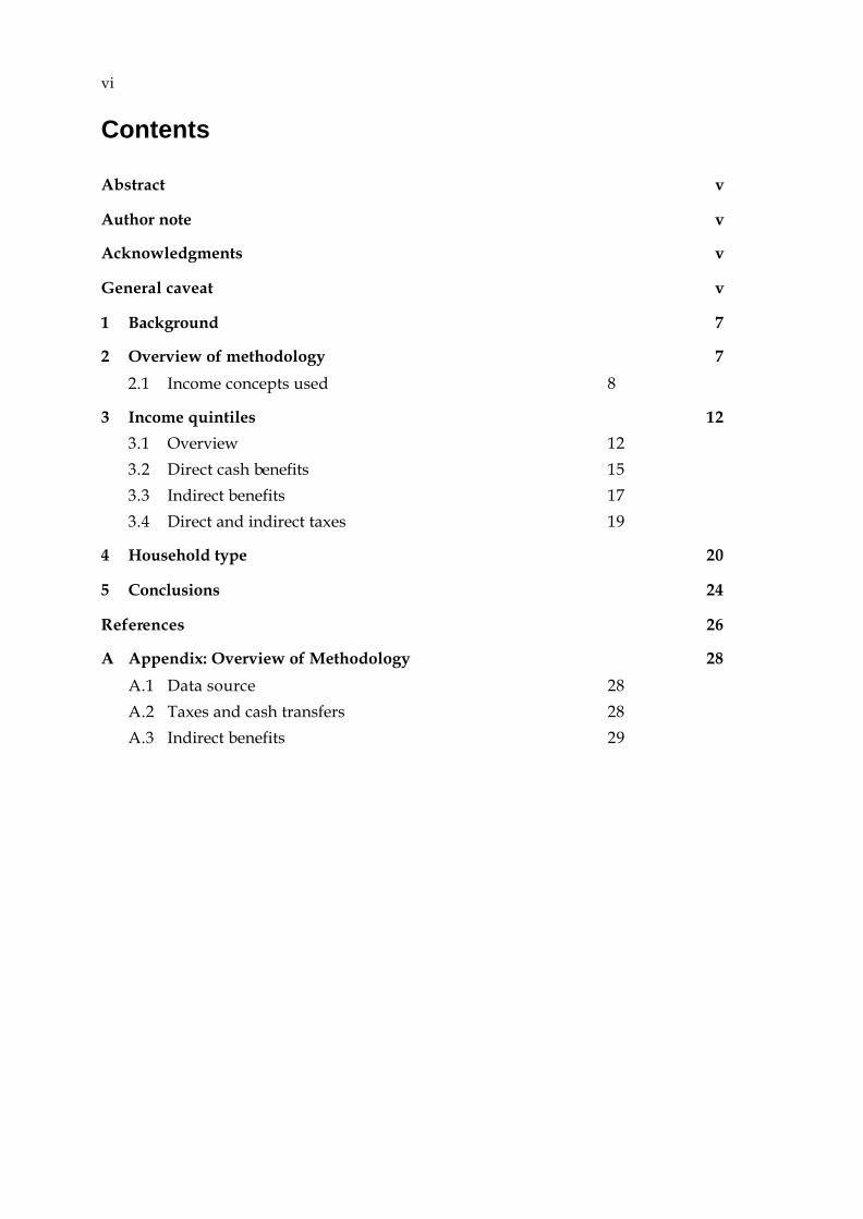
Contents

Abstract v

Author note v

Acknowledgments v

General caveat v

1 Background 7

2 Overview of methodology 7

2.1 Income concepts used 8

3 Income quintiles 12

3.1 Overview 12

3.2 Direct cash benefits 15

3.3 Indirect benefits 17

3.4 Direct and indirect taxes 19

4 Household type 20

5 Conclusions 24

References 26

A Appendix: Overview of Methodology 28

A.1 Data source 28

A.2 Taxes and cash transfers 28

A.3 Indirect benefits 29

NATSEM, University of Canberra 7

1 Background

Governments influence income distribution in many ways, including through an extensive web of regulatory and non-budgetary policies. However, the distribution of income is more directly affected through the billions of dollars of taxation revenue that government raises annually and the social programs upon which a large part of that revenue is spent. This study examines the distribution and redistribution of income in Australia in 2001-02.

This study is a fiscal incidence study, in that it attempts to estimate the impact of selected outlays and taxes upon the income distribution of households. This means that government outlays are attributed as a benefit to individual households, while taxes are attributed as a burden upon individual households.

Allocating the incidence of taxes and benefits is neither a straightforward nor an uncontroversial task. For example, fiscal incidence studies typically assume that the value of one year of primary education in a government school to a household containing such a primary school student is the cost to government of providing that year of education (Harding, 1984, ABS 2001a). But the cost to government may or may not approximate the value that a particular household places upon education, health or other government provided or subsidised services.

Similarly, the incidence of taxes is not uncontroversial. For example, is a tax levied upon companies shifted to consumers (via higher prices) or to shareholders (via lower dividends)? Equally, a tax collected in a jurisdiction such as Queensland (one of the states of Australia) may actually be incident upon international or interstate visitors, rather than upon Queensland households themselves.

Despite these continuing issues, fiscal incidence studies are now well established in both Australia and overseas (e.g. Harding, 1984 and 1995, Johnson et al, 1995, Raskall and Urquhart, 1994, Warren 1997). In particular, the Australian Bureau of Statistics (ABS) has now published a series of Fiscal Incidence Studies, which build upon the results in its Household Expenditure Surveys, and these now act as a benchmark for many Australian studies (1992, 1996, 2001).

2 Overview of methodology

It is important to appreciate that not all taxes and benefits are included within the scope of this study and that the results are heavily dependent upon the quality of the household sample survey data used (Siminski et al, 2003) and our assumptions about

8 NATSEM, University of Canberra

the usage and cost of government services. The benefits and taxes included are generally restricted to those that are relatable to particular types of households and/or household expenditure – or for which we had data to determine their incidence.

Household income is increased directly by benefits in the form of regular cash payments, such as the age pension and family payments, and indirectly by government expenditures such as those on health and education. On the other hand, household income is reduced by personal income taxes (direct taxes) and by indirect taxes passed on in the higher prices households pay for goods and services (ABS, 2001, p.3). Like the ABS fiscal incidence studies, this study excludes some government taxes and expenditures. On the revenue side, we have not considered such Commonwealth taxes as corporate taxes or any of the taxes levied by the various Australian states and territories. On the outlay side, we have not considered spending on such areas as defence, public safety, transport and communications.

In summary, this paper estimates the distribution in 2001-02 of:

• The major social security cash transfers and family payments;

• Income tax and selected income tax rebates and concessions, including the private health insurance rebate;

• The Commonwealth 10 per cent Goods and Services Tax (GST) plus excises on tobacco, alcohol, crude oil and LPG; and

• Health, housing, welfare and education non-cash benefits.

The methodology used in this study is described in more detail in Appendix A to this paper. The core data source used in the simulation of the 2001-02 world is the 1998-99 Household Expenditure Survey (HES) unit record file released by the Australian Bureau of Statistics. This file contains a snapshot of the demographic, labour force, income and other characteristics of the Australian population in 1998-99. It is important to note that the scope of the survey is restricted to those living in private dwellings and excludes those living in remote and sparsely settled areas. We made some adjustments to this file to update the private incomes, housing costs and population weights from 1998-99 to 2001-02 levels.

2.1 Income concepts used

A number of income concepts are used in this study, and these are summarised in Box 1. Original or private income is the most narrow definition of income used in the study, and comprises income from such sources as wages, superannuation,


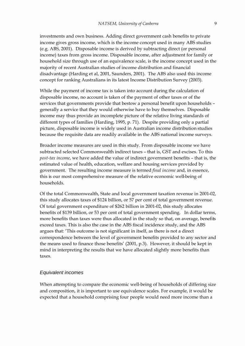
investments and own business. Adding direct government cash benefits to private income gives gross income, which is the income concept used in many ABS studies (e.g. ABS, 2001). Disposable income is derived by subtracting direct (or personal income) taxes from gross income. Disposable income, after adjustment for family or household size through use of an equivalence scale, is the income concept used in the majority of recent Australian studies of income distribution and financial disadvantage (Harding et al, 2001, Saunders, 2001). The ABS also used this income concept for ranking Australians in its latest Income Distribution Survey (2003).

While the payment of income tax is taken into account during the calculation of disposable income, no account is taken of the payment of other taxes or of the services that governments provide that bestow a personal benefit upon households – generally a service that they would otherwise have to buy themselves. Disposable income may thus provide an incomplete picture of the relative living standards of different types of families (Harding, 1995, p. 71). Despite providing only a partial picture, disposable income is widely used in Australian income distribution studies because the requisite data are readily available in the ABS national income surveys.

Broader income measures are used in this study. From disposable income we have subtracted selected Commonwealth indirect taxes – that is, GST and excises. To this post-tax income, we have added the value of indirect government benefits – that is, the estimated value of health, education, welfare and housing services provided by government. The resulting income measure is termed final income and, in essence, this is our most comprehensive measure of the relative economic well-being of households.

Of the total Commonwealth, State and local government taxation revenue in 2001-02, this study allocates taxes of $124 billion, or 57 per cent of total government revenue. Of total government expenditure of $262 billion in 2001-02, this study allocates benefits of $139 billion, or 53 per cent of total government spending. In dollar terms, more benefits than taxes were thus allocated in the study so that, on average, benefits exceed taxes. This is also the case in the ABS fiscal incidence study, and the ABS argues that: ‘This outcome is not significant in itself, as there is not a direct correspondence between the level of government benefits provided to any sector and the means used to finance those benefits’ (2001, p.3). However, it should be kept in mind in interpreting the results that we have allocated slightly more benefits than taxes.

Equivalent incomes

When attempting to compare the economic well-being of households of differing size and composition, it is important to use equivalence scales. For example, it would be expected that a household comprising four people would need more income than a


single person household if the two households were to enjoy the same standard of living. There is not, however, agreement internationally or nationally about exactly how much more income the four person household requires than the single person household to achieve the same standard of living. Like the recent ABS income distribution study (2003), our study uses the modified OECD equivalence scale. In our study, this means that we have given the first adult in each household a weight of 1.0, second and subsequent adults a weight of 0.5 points, and dependent children a weight of 0.3 points. The relevant cash income measure is then divided by the sum of the above points, to calculate the household’s equivalent income.

BOX 1: INCOME CONCEPTS AND STAGES OF REDISTRIBUTION

PRIVATE INCOME before government intervention (income from

employment, investment etc) BENEFITS TAXES

CASH BENEFITS (age pension, etc)

GROSS INCOME

DISPOSABLE INCOME

POST-TAX INCOME

FINAL INCOME

DIRECT TAXES

Plus

Minus

INDIRECT TAXES Minus

INDIRECT BENEFITS (education, health, etc)

Plus


It is not clear that equivalence scales designed for use with cash measures of economic well-being can be used when non-cash benefits (such as the value of education consumed) are included within the definition of income (Radner, 1994). The equivalence scales applied to cash income measures are intended to capture the economies of scale that occur when individuals share households (e.g. a couple living together require only one bed and fridge rather than the two required if they lived separately). Following Smeeding et al, we have assumed that there are no economies of scale in non-cash income (1993, p. 240). Most of the output tables in the following section show the total indirect (or non-cash) benefits received by different types of households. For our final measure of economic well-being, ‘equivalent final income’, we have added together equivalent post-tax income and per-capita indirect benefits income, following previous practice in studies of this kind (Smeeding et al, 1993, p. 241; Harding, 1995, p. 77).

Weighting

Another difficult issue is the appropriate ‘weight’ to use when analysing the results of our study. Consider two households, one containing four people and the other containing one person. If we use household weighting, then each household counts once when constructing our estimates. If we use person weighting, then the first household counts four times and the second household counts once. The second approach is considered theoretically the most appropriate, as it does not assume that people living in larger households are less important than people living in smaller households when assessing the income distribution. The ABS has just moved in its most recent income distribution publication to presenting some results for persons rather than for households (2003, p. 13).

In the output tables in the following section, when dividing the population into income quintiles, we have used quintiles of persons rather than quintiles of households. Thus, the bottom quintile consists of the bottom 20 per cent of Australians, rather than the bottom 20 per cent of households. Using person weighting to create the quintiles ensures that our measures are not unduly biased by differences in the average household size within different quintiles. As the ABS notes, this was a problem with their earlier fiscal incidence studies, in which they used quintiles of households rather than quintiles of persons (2001, p. 9).

Quite apart from the division of the population into income quintiles, another issue is whether the results included within each output table are person or household weighted. While person weighting might be considered the most desirable alternative theoretically, the results are then less accessible to the broad community. Accordingly, we have followed the practice used in the most recent fiscal incidence studies carried out by the ABS and UK Office for National Statistics, in presenting


averages for households within each output table (ABS, 2001, ONS, 2003). However, in the case of the three equivalent income measures presented in the following tables, the results are person weighted rather than household weighted. This is the same procedure followed by the ABS in its latest study of income distribution (2003, p. 37). In other words, only the three equivalent income measures in the following output tables for income quintiles are for persons rather than households.

3 Income quintiles

For this part of our study all Australians have been ranked by the equivalent disposable income of their household, and then divided into quintiles. The bottom quintile thus consists of the bottom 20 per cent of Australians, not the bottom 20 per cent of households.

3.1 Overview

Government intervention through the payment of taxes and the distribution of benefits narrows the gap between high and low income households in Australia. Looking at the private income of households, before direct intervention by government, the top quintile receive $2151 a week (Table 1 and Figure 1). This is about 43 times greater than the private incomes of the bottom quintile. After taking account of the taxes and benefits included within the scope of our study, the ratio between the final incomes of the top and bottom quintiles is reduced to three to one. Overall, the bottom 60 per cent of Australians are gainers from the tax and benefit programs considered here, with these gains being financed by the top 40 per cent of Australians. For the top 20 per cent of Australians, final income is 73 per cent of private income. For the bottom 20 per cent of Australians, final income is 10 times private income (Table 1).


Table 1 Estimated distribution of household income, taxes and benefits, by quintile of equivalent disposable household income, 2001-02

Note: The quintiles are for persons, ranked by the equivalent disposable income of their household. The bottom quintile thus consists of the bottom 20% of Australians. However, the values within the table are household averages (that is, the results in the table are household weighted rather than person weighted, so as to make interpretation of the results more comprehensible). The only exception to this are the three italicised equivalent income rows, where the results are person weighted to take account of the minor differences in average household size between the deciles.

Lowest 20%

Second Quintile

Middle 20%

Fourth Quintile

Highest 20% ALL

Private Income 47.2 377.1 809.9 1236.6 2051.5 893.5Direct Benefits 247.8 231.9 119.7 52.3 12.1 135.5Gross Household Income 295.0 609.1 929.6 1288.9 2063.6 1029.0Direct Tax 4.1 51.7 146.7 255.9 536.8 199.5

Disposable Income 290.9 557.3 783.0 1032.9 1526.9 829.6Selected Indirect Taxes 60.5 85.9 114.1 133.0 184.3 114.6Post-tax Income 230.5 471.5 668.9 899.9 1342.6 714.9

Selected Indirect Benefits 258.7 297.5 265.0 206.0 136.0 230.5 Total Education Benefits 66.4 106.0 111.7 92.3 53.3 83.4 Non-Government Schools 7.4 12.2 20.8 19.5 9.0 13.2 Government Schools 40.2 68.2 57.6 40.5 17.2 43.4 All Schooling 50.2 84.9 82.4 63.1 27.4 59.5 Tertiary 16.2 21.1 29.3 29.2 25.9 23.9

Total Health Benefits 118.9 127.6 109.4 92.6 77.9 105.1 Hospital Care 56.6 59.2 46.0 35.7 29.3 45.5 Medical Clinics 31.9 34.7 31.6 28.6 23.4 29.9 Pharmaceuticals 16.1 14.0 9.6 6.1 3.9 10.1 Other Health Benefits 11.2 15.1 15.9 15.2 13.0 13.9

PHI Rebate 3.1 4.7 6.4 7.0 8.2 5.8

Housing Benefits 12.8 3.2 1.2 0.4 0.3 4.1

Total Indirect Welfare Benefits 60.7 60.7 42.7 20.7 4.5 38.0 Child Care Benefits 3.5 7.3 4.6 2.0 0.3 3.4 Soc Sec & Welfare Services 57.1 53.4 38.1 18.7 4.2 34.6

Final Income 489.2 769.0 933.9 1105.9 1478.6 945.4Total Benefits Allocated 506.5 529.5 384.7 258.3 148.2 366.0Total Taxes Allocated 64.5 137.6 260.8 389.0 721.1 314.1Net Benefits Allocated 442.0 391.9 123.9 -130.7 -572.9 51.9

Equiv. Disposable Income 200.5 315.5 422.5 573.1 921.0 486.6Equiv After Housing Disposable Inc 154.0 262.2 362.5 504.2 826.1 421.9Equiv. Final Income 280.8 371.2 449.4 572.9 865.7 508.1

Persons per HH 2.13 2.86 3.01 2.82 2.4 2.6Adults per HH 1.58 1.87 2.06 2.09 2.06 1.91Number of Dependants per HH 0.55 0.99 0.95 0.73 0.35 0.69Number Aged 65+ Per HH 0.49 0.47 0.29 0.16 0.09 0.3Total No of Households '000 1807.2 1344.7 1282.3 1369.7 1607.1 7410.9

Quintile of Equivalent Household Disposable Income

Average $ per week per household


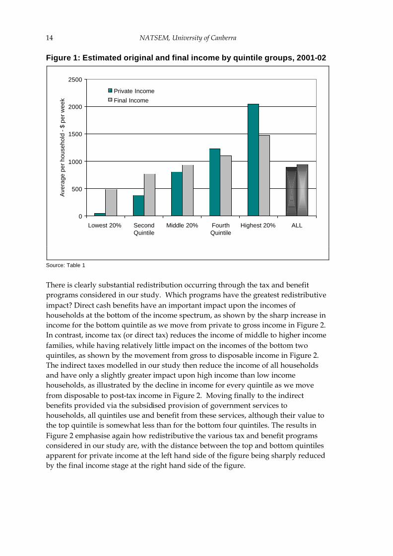
Figure 1: Estimated original and final income by quintile groups, 2001-02

0

500

1000

1500

2000

2500

Lowest 20% SecondQuintile

Middle 20% FourthQuintile

Highest 20% ALL

Ave

rage

per

hou

seho

ld -

$ pe

r wee

k

Private Income

Final Income

Source: Table 1

There is clearly substantial redistribution occurring through the tax and benefit programs considered in our study. Which programs have the greatest redistributive impact? Direct cash benefits have an important impact upon the incomes of households at the bottom of the income spectrum, as shown by the sharp increase in income for the bottom quintile as we move from private to gross income in Figure 2. In contrast, income tax (or direct tax) reduces the income of middle to higher income families, while having relatively little impact on the incomes of the bottom two quintiles, as shown by the movement from gross to disposable income in Figure 2. The indirect taxes modelled in our study then reduce the income of all households and have only a slightly greater impact upon high income than low income households, as illustrated by the decline in income for every quintile as we move from disposable to post-tax income in Figure 2. Moving finally to the indirect benefits provided via the subsidised provision of government services to households, all quintiles use and benefit from these services, although their value to the top quintile is somewhat less than for the bottom four quintiles. The results in Figure 2 emphasise again how redistributive the various tax and benefit programs considered in our study are, with the distance between the top and bottom quintiles apparent for private income at the left hand side of the figure being sharply reduced by the final income stage at the right hand side of the figure.


Figure 2 Income stages by quintile group, 2001-02

2064

1527

13431479

295 291 230

489

2051

47

0

500

1000

1500

2000

2500

PrivateIncome

GrossHousehold

Income

DisposableIncome

Post-taxIncome

FinalIncome

Ave

rage

per

hou

seho

ld -

$ pe

r wee

k

Highest 20%

FourthQuintile

Middle 20%

SecondQuintile

Lowest 20%

Source: Table 1

3.2 Direct cash benefits

The extent of redistribution is again underlined in Figure 3, which shows clearly that it is cash and non-cash benefits that are particularly important in boosting the incomes of the bottom three quintiles and taxes that are more significant in reducing the incomes of the top quintile. Direct benefits are heavily concentrated upon the bottom two quintiles, amounting to between about $230 and $250 a week (Table 1). In contrast, direct benefits amount to only $12.10 a week for the top quintile. This indicates that direct benefits are highly progressive, amounting to 84 per cent of the gross income of the bottom quintile and then falling rapidly to only 0.6 per cent of the gross income of the top quintile (Figure 4). This very high degree of progressivity reflects the tightly targeted nature of direct transfers in Australia, in contrast to the social insurance systems of many European countries. Australian cash transfers are generally both income and asset tested and their level depends only upon current private income and wealth, rather than upon previous workforce experience. Moreover, the private income definition adopted under the welfare system is more comprehensive than that under the personal income tax.


Figure 3 Summary of the estimated effects of taxes and benefits by quintile group, 2001-02

-800

-600

-400

-200

0

200

400

600



Highest 20%

Ave

rage

per

hou

seho

ld -

$ pe

r

Indirect Benefits

Direct Benefits

Direct Taxes

Indirect Taxes

Figure 4 Estimated benefits received as a percentage of gross income, by quintile group, 2001-02

171.7

86.9

6.6

87.7

0.6

84.0

41.4

7.220.0

0

20

40

60

80

100

120

140

160

180



Highest 20%

%

Indirectbenefits

Cashbenefits

Allbenefits


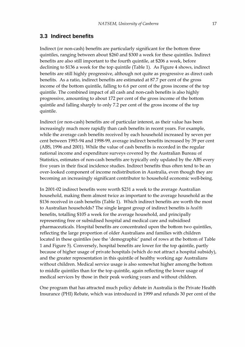
3.3 Indirect benefits

Indirect (or non-cash) benefits are particularly significant for the bottom three quintiles, ranging between about $260 and $300 a week for these quintiles. Indirect benefits are also still important to the fourth quintile, at $206 a week, before declining to $136 a week for the top quintile (Table 1). As Figure 4 shows, indirect benefits are still highly progressive, although not quite as progressive as direct cash benefits. As a ratio, indirect benefits are estimated at 87.7 per cent of the gross income of the bottom quintile, falling to 6.6 per cent of the gross income of the top quintile. The combined impact of all cash and non-cash benefits is also highly progressive, amounting to about 172 per cent of the gross income of the bottom quintile and falling sharply to only 7.2 per cent of the gross income of the top quintile.

Indirect (or non-cash) benefits are of particular interest, as their value has been increasingly much more rapidly than cash benefits in recent years. For example, while the average cash benefits received by each household increased by seven per cent between 1993-94 and 1998-99, average indirect benefits increased by 39 per cent (ABS, 1996 and 2001). While the value of cash benefits is recorded in the regular national income and expenditure surveys covered by the Australian Bureau of Statistics, estimates of non-cash benefits are typically only updated by the ABS every five years in their fiscal incidence studies. Indirect benefits thus often tend to be an over-looked component of income redistribution in Australia, even though they are becoming an increasingly significant contributor to household economic well-being.

In 2001-02 indirect benefits were worth $231 a week to the average Australian household, making them almost twice as important to the average household as the $136 received in cash benefits (Table 1). Which indirect benefits are worth the most to Australian households? The single largest group of indirect benefits is health benefits, totalling $105 a week for the average household, and principally representing free or subsidised hospital and medical care and subsidised pharmaceuticals. Hospital benefits are concentrated upon the bottom two quintiles, reflecting the large proportion of older Australians and families with children located in these quintiles (see the ‘demographic’ panel of rows at the bottom of Table 1 and Figure 5). Conversely, hospital benefits are lower for the top quintile, partly because of higher usage of private hospitals (which do not attract a hospital subsidy), and the greater representation in this quintile of healthy working age Australians without children. Medical service usage is also somewhat higher among the bottom to middle quintiles than for the top quintile, again reflecting the lower usage of medical services by those in their peak working years and without children.

One program that has attracted much policy debate in Australia is the Private Health Insurance (PHI) Rebate, which was introduced in 1999 and refunds 30 per cent of the


cost of private health insurance. We estimate that the PHI rebate was worth an average of $3.10 a week to bottom quintile households, rising to $8.20 a week for top quintile households. However, perhaps surprising many, the PHI rebate is still progressive, amounting to a higher proportion of the gross income of bottom quintile households than of top quintile households (1.0 per cent vs 0.4 per cent). This is because the rebate is more evenly distributed than is gross income. Despite this, more than half of all spending on the rebate is received by the top 40 per cent of Australians, with the bottom 40 per cent receiving only 28 per cent of total outlays on the rebate (Table 1).

As found in previous studies (Harding et al, 2004), the Australian Pharmaceutical Benefits Scheme, described briefly in the Appendix, is highly progressive, with its benefits being heavily targeted towards low income concession card holders. Average pharmaceutical benefits for the top quintile are only $3.90 a week — or only one-quarter of those received by the bottom quintile (Table 1 and Figure 5).

Education is the second big-ticket indirect benefit item, representing $83 a week to the average Australian household. While state government outlays on education tend to be directed towards government schools, the subsidy by the Federal government to non-government schools has been increasing more rapidly than that to government schools in recent years, arousing some controversy (AEU, 2004)

Figure 5 Estimated indirect benefits received, by quintile group, 2001-02

0

50

100

150

200

250

300

350

Lowest20%

SecondQuintile

Middle20%

FourthQuintile

Highest20%

$ p

er w

eek

Welfare and Housing

Other Health Benefits

Pharmaceuticals

Medical Services

Hospital Care

Tertiary Education

Government Schools

Non Government Schools


Looking at all government outlays on education together, government school subsidies are much more redistributive towards lower income families than non-government school subsidies, with just over half of all outlays on government schools being directed towards the bottom two quintiles, compared with only 30 per cent of all non-government school outlays. School outlays as a whole are concentrated on the bottom three quintiles, who receive 70 per cent of total school outlays. Expenditure on tertiary students is somewhat skewed towards the top three quintiles, as shown in Figure 5.

The remaining category of non-cash benefits considered is welfare services and housing benefits. Housing benefits are the most progressive of all the non-cash benefits considered in Table 1, but total spending on public housing is much lower than for the other services considered here, so they have been grouped with welfare services in Figure 5. Welfare services are a rapidly growing category of government expenditure and, as Figure 5 illustrates, one that is of major benefit to lower income Australians.

3.4 Direct and indirect taxes

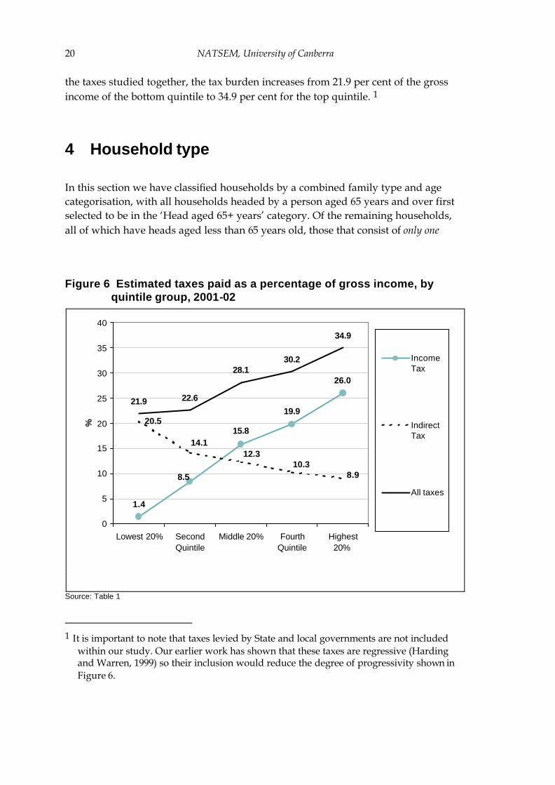
Moving now to the tax side, as Figure 3 shows graphically, it is the direct tax paid by the top quintile that is particularly striking and an important contributor to the overall redistributive impact of tax and benefit programs. The direct tax paid by the top quintile of about $537 a week is more than double the average direct tax of $256 a week paid by the fourth quintile and about 3.6 times the average direct taxes of $147 a week paid by the middle quintile (Table 1). This suggests that income tax in Australia is highly progressive and this is confirmed in Figure 6, which shows that income tax as a percentage of gross income rises sharply from 1.4 per cent for the bottom quintile to 15.8 per cent for the middle quintile and 26 per cent for the top quintile.

On the other hand, the indirect taxes considered in our study (GST and excise duties) are regressive. As Figure 3 shows, all quintiles pay indirect taxes and the magnitude of the indirect taxes paid shows relatively little variation with income, with the $184 of indirect taxes paid each week by the top quintile amounting to only triple the $61 a week paid by the bottom quintile (Table 1). The selected indirect taxes amount to an estimated 20.5 per cent of the gross income of the bottom quintile, falling to only 8.9 per cent of the gross income of the top quintile (Figure 6).

While the progressive impact of income tax in Australia is partially offset by the regressive impact of GST and excise duties, the overall impact of the taxes considered in our study remains progressive. As Figure 6 illustrates, considering all


the taxes studied together, the tax burden increases from 21.9 per cent of the gross income of the bottom quintile to 34.9 per cent for the top quintile. 1

4 Household type

In this section we have classified households by a combined family type and age categorisation, with all households headed by a person aged 65 years and over first selected to be in the ‘Head aged 65+ years’ category. Of the remaining households, all of which have heads aged less than 65 years old, those that consist of only one

Figure 6 Estimated taxes paid as a percentage of gross income, by quintile group, 2001-02

1.4

15.8

19.920.5

21.9 22.6

28.130.2

34.9

8.5

26.0

8.910.3

14.112.3

0

5

10

15

20

25

30

35

40



Highest20%

%

IncomeTax

IndirectTax

All taxes

Source: Table 1

1 It is important to note that taxes levied by State and local governments are not included

within our study. Our earlier work has shown that these taxes are regressive (Harding and Warren, 1999) so their inclusion would reduce the degree of progressivity shown in Figure 6.


income unit were identified and classified into family types.2 For example, a ‘Couple only’ household consists here of only two people, living as a couple. If such couples live with non-dependent children, other relatives, or unrelated individuals, then they are placed within the ‘Other’ category. Similarly, ‘Couples with dependent children’ includes only those households that consist of couples and their dependent children. Again, if such households also include non-dependent children, other relatives or unrelated individuals, then such couples are placed into the ‘Other’ household category. The ‘Other’ household category thus consists of all multiple income unit and/or multiple family households, including group households, all non-dependent children living with their parents, and two or more families sharing the same household.

Of the household types considered in Table 2, the final incomes of aged and sole parent households are affected the most by the redistribution created by the Australian welfare state (Figure 7). In 2001-02 the average private incomes of aged households are about $220 a week, and are then roughly doubled by the receipt of cash transfers – predominantly the age pension. Aged households also receive substantial amounts of indirect benefits – and particularly health benefits. Sole parent households receive almost $300 a week in private income, with almost another $300 being added to this in direct benefits, principally via parenting payment. Sole parents receive about another $340 a week in indirect benefits, mainly via the provision of government schooling and health benefits.

Couples with children are on average marginal gainers from the operation of the Australian welfare state, with their relatively high receipt of education and health indirect benefits being largely offset by their direct and indirect tax payments. Couples without children are net payers from the taxes and outlays considered in our study, with their direct and indirect taxes greatly exceeding their direct and indirect benefits. Single person households are also net payers, although not to the same extent as couples without children. However, it must be appreciated that couple without children households consist of two people while single person households by definition consist of only one person. On a per capita basis, the net loss from the welfare state is only slightly higher for couple only households than for single person households. The average benefits received by ‘other’ households are roughly balanced by their average taxes (Figure 8).

2 An income unit is defined by the ABS as a person or group of related persons living within

a household, whose command over income is assumed to be shared. Income sharing is considered to take place within married (registered or de facto) couples, and between parents and dependent children. Dependent children are defined as children aged under 15 years, and people aged 15-24 years who are full-time students, live with one or both of their parents, and do not have a partner or child of their own in the household.


Figure 7 Income stages by household type, 2001-02

0

200

400

600

800

1000

1200

1400

1600

PrivateIncome

GrossHousehold

Income

DisposableIncome

Post-taxIncome

FinalIncome

$ p

er w

eek

Other

Couplewith DepChildrenCoupleOnly

SoleParent

SinglePerson

Head Aged65+ Years

Figure 8 Summary of the estimated effects of taxes and benefits, by household type, 2001-02

-500

-300

-100

100

300

500

700

Head Aged65+ Years

CoupleOnly

Couple withDep

Children

Sole Parent SinglePerson

Other

$ pe

r w

eek

Indirect BenefitsDirect BenefitsDirect TaxesIndirect Taxes


Table 2 Estimated distribution of household income, taxes and benefits, by household type, 2001-02

Head Aged 65+

Years Couple

Only

Couple with Dep Children

Sole Parent

Single Person Other ALL

Private Income 218.5 1134.6 1217.0 296.1 594.2 1242.8 893.5Direct Benefits 225.0 49.1 115.9 298.0 55.2 167.4 135.5Gross Household Income 443.5 1183.7 1332.9 594.1 649.4 1410.2 1029.0Direct Tax 27.5 256.4 293.2 58.1 147.2 260.3 199.5

Disposable Income 416.1 927.3 1039.7 536.0 502.2 1150.0 829.6Selected Indirect Taxes 66.1 122.9 141.3 70.3 68.2 160.4 114.6Post-tax Income 350.0 804.4 898.4 465.7 433.9 989.6 714.9

Selected Indirect Benefits 222.9 114.0 354.3 340.6 75.2 270.4 230.5 Total Education Benefits 0.4 15.6 199.0 189.6 12.3 96.9 83.4 Non-Government Schools 0.1 0.0 40.7 25.7 0.0 9.5 13.2 Government Schools 0.1 0.3 118.5 134.3 0.0 35.9 43.4 All Schooling 0.2 0.3 168.3 168.0 0.0 47.1 59.5 Tertiary 0.2 15.2 30.7 21.6 12.3 49.7 23.9

Total Health Benefits 158.5 81.0 109.7 80.3 41.9 126.5 105.1 Hospital Care 98.0 31.5 35.9 26.0 17.5 49.5 45.5 Medical Clinics 29.0 24.7 37.4 26.2 12.6 39.3 29.9 Pharmaceuticals 19.1 7.2 7.4 10.1 3.9 12.4 10.1 Other Health Benefits 7.9 10.7 21.5 14.9 5.4 18.2 13.9 PHI Rebate 4.5 6.9 7.4 3.0 2.5 7.2 5.8

Housing Benefits 5.1 1.3 1.5 17.0 6.4 3.2 4.1

Total Indirect Welfare Benefits 58.9 16.1 44.1 53.8 14.6 43.8 38.0 Child Care Benefits 0.0 0.0 10.5 12.4 0.0 1.2 3.4 Soc Sec & Welfare Services 58.9 16.1 33.7 41.4 14.6 42.6 34.6

Final Income 572.9 918.4 1252.7 806.2 509.1 1260.0 945.4Total Benefits Allocated 448.0 163.0 470.2 638.6 130.4 437.8 366.0Total Taxes Allocated 93.5 379.3 434.5 128.4 215.4 420.7 314.1Net Benefits Allocated 354.4 -216.2 35.7 510.2 -85.1 17.2 51.9

Equiv. Disposable Income 337.0 618.2 470.3 333.1 502.2 527.9 486.6Equiv After Housing Disposable Inc 366.6 805.2 893.7 419.2 401.5 1028.3 717.9Equiv. Final Income 432.4 593.3 494.2 412.4 509.1 533.0 508.1

Persons per HH 1.5 2.0 4.0 2.8 1.0 3.4 2.6Adults per HH 1.5 2.0 2.0 1.0 1.0 3.0 1.9Number of Dependants per HH 0.0 0.0 2.0 1.8 0.0 0.5 0.7Total No of Households '000 1265.5 1204.4 1760.0 397.6 1141.2 1642.2 7410.9

Average $ per week per household

Quintile of Equivalent Household Disposable Income


5 Conclusions

This study assesses the distribution of household income and selected taxes and benefits in 2001-02. Fiscal incidence studies such as this rely on sample survey data and make assumptions about the patterns of receipt and value of various types of benefits and about the payment of selected types of taxes. We faced numerous difficulties with both the sample survey data underlying the study and with the benchmark data used to estimate the taxes received by government and the outlays expended by government. It is also important to appreciate that the benefits and taxes included in our study are generally restricted to those that are either relatable to particular types of households or to household expenditure — or for which we have data to determine their incidence. While we have imputed income tax, the Goods and Services Tax and excises in 2001-02, we have not imputed the incidence of such other taxes as capital gains tax, company tax, indirect taxes levied by the States and Territories, and superannuation tax concessions. Similarly, while we have imputed the usage and value of government health, education, housing and welfare outlays that relate directly to particular types of households, we have not included other government outlays such as spending on defence or communications. With these caveats in mind, our study uses a similar methodology to that of other fiscal incidence studies, including those by the Australian Bureau of Statistics (2001) and the UK Office for National Statistics (2003).

Our study has shown that there is extensive redistribution between households due to the operation of the Australian system of taxes and benefits. This is not unexpected, as this is an intended consequence of the programs of taxes and services included within our study. Our welfare state system has been designed to assist those in our community who are most in need of support. It has also been designed to assist households through the course of their lifecycle, by redistributing income from periods of relative affluence during the lifecycle to periods of relative greater need, such as when there are children or in retirement.

The net impact of the taxes and benefits included within our study is to redistribute income from the most affluent 40 per cent of Australians to the less affluent 60 per cent. In particular, there is substantial redistribution via the income tax system from the top 20 per cent of Australians to the bottom 60 per cent. The income tax system is progressive, taking a greater proportion of the gross income of higher income households. The indirect taxes (GST and excise duties) included in our study amount to a much smaller proportion of the income of high income households, although in


dollar terms the top income quintile pay three times as much in indirect tax as the bottom income quintile. While the indirect taxes included within our study are regressive, this is not sufficient to offset the impact of direct taxes so the combined effect of all the direct and indirect taxes included here remains progressive.

Direct (or cash) transfers in Australia are also very progressive, with three-quarters of total outlays being received by the bottom two income quintiles. While outlays on indirect (or non-cash) benefits are less pro-poor in their impact than this, they are nonetheless also still progressive. Taking both direct and indirect benefits, the bottom two quintiles receive about 60 per cent of total outlays, while the top two quintiles receive only 22 per cent of total outlays.

The impact of the welfare state also varies greatly by household type, with older Australians and sole parents emerging as the biggest gainers from redistribution. Interestingly, while there is substantial redistribution towards lower income couples with children, on average couples with children are not net gainers from the taxes and benefits considered in our study. In recent years the incomes of many such families in Australia have been boosted by falling unemployment and increasing participation in the workforce on a full or part time basis by both parents. This has led to rising income tax payments for couples with children, offsetting the education and health benefits generated by the presence of children. Couples without children, single person households and ‘other’ households remain net losers from the taxes and benefits considered in our study.


References

ABS 2003, Cat. No. 6523.0, Household Income and Its Distribution, Australia, 2000-01, July.

ABS 2001, Cat. No. 6537.0, Government Benefits, Taxes and Household Income 1998-99, August 2001.

ABS 1996, Cat. No. 6537.0, 1993-94 Household Expenditure Survey, Australia: The Effects of Government Benefits and Taxes on Household Income.

ABS 1992, Cat. No. 6537.0, 1998-89 Household Expenditure Survey, Australia: The Effects of Government Benefits and Taxes on Household Income.

Australian Education Union (AEU) 2004, Submission to the Senate Inquiry into Commonwealth Funding for Schools, http://www.aph.gov.au/Senate/committee/eet_ctte/schoolfunding/submissions/sub033.pdf (accessed 8 July 2004).

Bremner, K., Beer, G., Lloyd, R., and Lambert, S.-,2002, ‘Creating a Basefile for STINMOD’, Technical Paper No. 27, National Centre for Social and Economic Modelling, University of Canberra , June

Department of Family and Community Services (FaCS) 1999, Annual Report 1998-99, Canberra.

Department of Family and Community Services (FaCS) 2002, Annual Report 2001-02, Canberra.

Harding, A, Abello, A, Brown, L, and Phillips, B, 2004, The Distributional Impact of Government Outlays on the Australian Pharmaceutical Benefits Scheme in 2001-02, Economic Record, Vol 80, Issue S1, September.

Harding, A, Lloyd, R, Greenwell, H, 2001, Financial Disadvantage in Australia 1900 to 2000: The persistence of poverty in a decade of growth, The Smith Family, Camperdown, NSW.

Harding, A, Percival, R, Schofield, D, Walker, A, 2000, ‘The Lifetime Distributional Impact of Government Health Outlays’, Discussion Paper No. 47, National Centre for Social and Economic Modelling, University of Canberra.

Harding, A and Warren, N, 1999, ‘Who Pays the Tax Burden In Australia?’, Discussion Paper No. 39, National Centre for Social and Economic Modelling, University of Canberra

Harding, A, 1995, ‘The impact of health, education and housing outlays upon income distribution in Australia in the 1990s’, Australian Economic Review, 3rd quarter, pp. 71-86.

Harding, A, 1984, Who Benefits?: The Australian Welfare Sate and Redistribution, Social Welfare Research Centre Reports and Proceedings no. 45, University of New South Wales, Sydney.


Johnson, D, Manning, I and Hellwig, O, 1995, ‘Trends in the Distribution of Cash and Non-Cash Benefits’, Report to the Department of Prime Minister and Cabinet, AGPS, Canberra, December.

Office of National Statistics (United Kingdom), 2003, The Effects of Taxes and Benefits on Household Income, 2001-02, (available from www.ons.gov.uk)

Radner, D (1994), Noncash Income, Equivalence Scales, and the Measurement of Economic Well-Being, Working Paper No. 63, Office of Research and Statistics, US Department of Health and Human Services, Washington, DC.

Raskall, P and Urquhart, R 1994, ‘Inequality, Living Standards and the Social Wage During the 1980s, Study of Social and Economic Inequalities, Monograph no.3, University of New South Wales, Sydney.

Saunders, P, 2001, ‘Household income and its distribution’, in Australian Bureau of Statistics, Australian Economic Indicators, Cat. No. 1350.0, ABS, Canberra, pp. 33–55.

Siminski, P., Saunders, P., Waseem, S. and Bradbury, B., 2003, ‘Assessing the Quality and Inter-Temporal Comparability of ABS Household Income Distribution Survey Data’, Discussion Paper No 123, Social Policy Research Centre, University of NSW.

Smeeding, T.M., Saunders, P., Coder, J., Jenkins, S., Fritzell J., Hagenaars, A.J.M., Hauser, R. and Wolfson, M., 1993, ‘Poverty, inequality and family living standards impacts across seven nations: the effect of non-cash subsidies for health, education and housing’, Review of Income and Wealth, Series 39, Number 3, pp. 229–56.

Warren, N, 1997, ‘Recent Trends in Taxation in Australia and their Impact on Australian Tax Incidence’, in J G Head and R. Krever, (eds.), Taxation Towards 2000, Conference Series 19, Australian Tax Research Foundation, Sydney.


A Appendix: Overview of Methodology

A.1 Data source

The core data source used in the simulation of the 2001-02 world is the 1998-99 Household Expenditure Survey (HES) confidentialised unit record file released by the Australian Bureau of Statistics. This file contains a snapshot of the demographic, labour force, income and other characteristics of the Australian population in 1998-99. It is important to note that the scope of the survey is restricted to those living in private dwellings and excludes those living in remote and sparsely settled areas. We made adjustments to this file to update the private incomes and housing costs of households to estimated 2001-02 levels, using such inflators as average weekly earnings and housing consumer price indexes. We also adjusted the population weights from 1998-99 to 2001-02 levels to allow for the four per cent growth in population that occurred over that period. We did not reweight the entire 1998-99 survey to account for possible changes in, for example, labour force and demographic status.

A.2 Taxes and cash transfers

In July 2000 Australia introduced a complex tax-mix shift towards indirect taxes, accompanied by extensive social security reforms. As a result, the declared values of these items in the 1998-99 Household Expenditure Survey were redundant. Accordingly, we had to impute the rules of the income tax and social security systems to estimate the income taxes paid by and the transfers received by each of the households in the HES file. This aspect of the modelling employed NATSEM’s STINMOD model, which is a long-established static microsimulation model of the Australian tax and transfer system used by government departments for budget policy formulation (Bremner et al, 2002).

The income tax system in Australia in 2001-02 consists of a tax threshold of $6000 and three further marginal tax rate thresholds above that, with the top marginal rate of 47 cents in the dollar cutting in at $60,000 of taxable income. There is also a Medicare levy of 1.5 per cent of taxable income, making the effective top marginal tax rate 48.5 per cent. There are no social insurance levies on top of this, with the Australian system of means-tested cash payments being financed from general revenue. Australia has a wide range of means-tested payments payable to the aged, unemployed, disabled, sick, sole parents, and families with children. These payments are essentially based on income and assets at the time of payment and,


unlike the European social insurance schemes, do not bear any relation to earlier earnings received while in the workforce.

To simulate the impact of the GST and excises we calculated the average tax rates applying to each of the 500 plus detailed expenditure categories contained within the HES for each household. Taxes initially borne by government or business are assumed to be shifted ultimately to consumers, either residents or non-residents. (This differs from the ABS fiscal incidence studies, which only allocate to households those indirect taxes that can be directly assigned to households through their final consumption expenditure.) However, like the ABS, we do not match national accounts estimates of GST and excises collected exactly, because of scope exclusions in the HES and under-statement of tobacco and alcohol consumption by households within the HES.

A.3 Indirect benefits

Moving now to indirect benefits, which consist of goods and services provided free or at subsidised prices by the government, our allocation of indirect benefits was restricted, as in the ABS studies (2001), to those arising from the provision of education, health, housing, and welfare services. In most cases, the estimation of the value of an indirect (or non-cash) benefit to households within the HES essentially consists of the following three steps:

• Identifying those households who are likely to use the service in question and calculating how often they use it within a year;

• Estimating the cost to government of that usage; and

• Multiplying the ‘amount of usage’ by the ‘cost to government’ to derive the annual estimated value then imputed to the household.

Education benefits

The ABS included on the 1998-99 HES unit record file its estimate of the value of each of the following education services consumed by each household in 1998-99: pre-school, primary and secondary school (divided into government and non-government schools), university, ‘technical and further education’, ‘tertiary education not elsewhere classified’ and ‘other education’. We inflated each of these values from their 1998-99 level to 2001-02 estimates, using the best inflator that we could find (generally the percentage change in average benefit per student, derived from such sources as Government Finance Statistics (GFS) and the Ministerial Council on Education, Employment, Training and Youth Affairs).


Health benefits

Health benefits are allocated for hospital care, medical clinics, pharmaceuticals, and other health benefits. Hospital care covers expenses relating to acute care institutions, medical clinics cover community health services, pharmaceuticals covers pharmaceuticals, medical aids and appliances, and other health benefits covers public health services, health research and health administration n.e.c.

In our study we calculated new estimates of the value of hospital and medical services and pharmaceuticals consumed. This was either because the program rules had changed so much between 1998-99 and 2001-02 that it was no longer appropriate to use the ABS estimates for 1998-99 or because we wished to use a more sophisticated imputation methodology.

The likelihood of using hospital and medical services was calculated from the 2001 National Health Survey (NHS), and based on such predictive characteristics as age, gender, income quintile and whether the household had private health insurance. Private and public hospital usage was modelled separately, as the latter are far more costly to government.

The likelihood of using prescribed pharmaceuticals was calculated from the 1995 National Health Survey (because the 2001 NHS did not include information on all pharmaceuticals). The Australian Pharmaceutical Benefit Scheme provides highly subsidised pharmaceuticals to ‘concession card holders’ (generally families and singles on low incomes), with a co-payment per script for this group of $3.50. For other Australians the patient meets the first $21.90 per script and the government meets the full cost of pharmaceuticals listed on the Scheme above this level. We modelled eligibility for concession cards in detail.

To estimate a value for ‘other health benefits’ we simply inflated the appropriate ABS estimate by the change in ‘other health’ shown in government finance statistics from 1998-99 to 2001-02, after adjustment for changes in population size.

Private Health Insurance Rebate

One of the innovative features of this study was the simulation of the distributional impact of the Private Health Insurance (PHI) Rebate in the 2001-02 world. The PHI rebate was not simulated by the ABS in its 1998-99 Fiscal Incidence study, as it was only introduced in 1999 (ABS, 2001). First, the probability of a person having private health insurance was estimated (from the 2001 NHS unit record file) by state, age, sex, income unit type and equivalent gross income unit income quintile. These likelihood estimates were then applied to persons in the HES and used to adjust the numbers in each sub-group who held insurance to match the proportions in the 2001


NHS. We then predicted whether the entire household were likely to be covered by private health insurance or just that individual, using administrative data. We then estimated the average amount paid for such private health insurance (before the rebate), from the amounts indicated on the HES and Private Health Insurance Administrative Council administrative data. Finally, the estimated amount of the PHI rebate was then calculated as 30 per cent of the pre-rebate cost of insurance.

Housing Benefits

Government expenses relating to housing largely involve building new houses for rent at subsidised cost. These expenses were not allocated amongst HES households in the ABS FIS study because “it is difficult to identify likely future recipients of the benefits” (2001, p. 51). Instead, benefits were allocated to households in government rental accommodation according to the value of their rent subsidy. The value of their rent subsidy was taken to be the difference between the rent paid by the households and the estimated value of private market rent according to the State, region, type of dwelling and number of bedrooms. To derive estimates for 2001-02 we multiplied the public housing benefits calculated by the ABS in the HES by the change in the housing Consumer Price Index (CPI) by State over the 1998-99 to 2001-02 period.

Other Welfare Services

These services exclude cash transfers (dealt with above) and comprise various publicly funded services to assist those who are disabled, aged, have children and so on. In 1998-99 the ABS calculated average indirect benefits for different types of benefit recipients, by dividing indirect welfare GFS expenses by the number of recipients of benefits. Different levels of benefit were calculated for persons receiving age, veterans affairs, and disability support pensions, and family allowance and parenting payment. Average benefits were allocated to persons receiving similar direct government benefits. Household benefits were the sum of household member benefits. To capture the change in these benefits between 1998-99 and 2001-02, we inflated by the change in total indirect welfare GFS expenses between the two years.

Child Care

Expenditure on child care assistance was treated separately by the ABS, and allocated to households with children under 12, according to household income and the probability that the children were attending eligible child care. While there was an apparent major change in child care assistance between 1998-99 and 2001-02 with the GST tax reform package, the rules of the old schemes were effectively largely replicated in the new Child Care Benefit. Accordingly, we simply inflated the child


care benefits shown in the ABS FIS by the change in total spending on child care benefits derived from the relevant departmental Annual Reports (FaCS, 1999, 2002).

Documents

The Distribution of Taxes and Government Benefits … Centre for Social and Economic Modelling • University of Canberra • The Distribution of Taxes and Government Benefits in Australia