Embed Size (px)
Citation preview

THE DETECTION OF OH-MASER SATELLITE LINES
IN HIGH MASS STAR FORMING REGIONS
by
Derek Felli
A senior thesis submitted to the faculty of
Brigham Young University
in partial fulfillment of the requirements for the degree of
Bachelor of Science
Department of Physics and Astronomy
Brigham Young University
April 2011

Copyright c© 2011 Derek Felli
All Rights Reserved

BRIGHAM YOUNG UNIVERSITY
DEPARTMENT APPROVAL
of a senior thesis submitted by
Derek Felli
This thesis has been reviewed by the research advisor, research coordinator,and department chair and has been found to be satisfactory.
Date Victor Migenes, Advisor
Date Eric Hintz, Research Coordinator
Date Scott Sommerfeldt, Chair

ABSTRACT
THE DETECTION OF OH-MASER SATELLITE LINES
IN HIGH MASS STAR FORMING REGIONS
Derek Felli
Department of Physics and Astronomy
Bachelor of Science
Microwave amplification by stimulated emission of radiation (MASER) orig-
inates from molecules which have been pumped to an excited state. Galactic
MASER emission originates from dense hot clumps of molecular gas. MASERs
are found in star forming regions (SFR), supernova remnants, and late-type
stars. There are various very well known MASER species OH-, H2O, CH3OH,
SiO, and H2CO to name some of the most common.
In this work we present the result of studying 41 galactic OH-MASERs using
the Very Large Baseline Array (VLBA). Common transitions observed in OH-
MASERs are the lines 1612, 1665, 1667, and 1720 MHz. The 1665 and 1667
MHz transitions are more common in SFR and are referred to as “main lines”
in the literature. The 1612 and 1720 MHz transitions are common in late-type
stars and are known as “satellite lines”. Generally 1612 and 1720 MHz lines

are not found in SFR. We studied these four transitions previously mentioned
in OH-MASERs, with very high spatial and spectral resolution. We were the
first to obtain high resolution observations for 1612 and 1720 MHz transitions
in many OH-MASER sources. From our data we determined that the 1720
MHz line strength is correlated of the star formation processes in high-mass
and low-mass SFR. Of the 41 sources 5 (11.4%) showed 1612 MHz lines and 10
(22.7%) showed 1720 MHz line. This correlation between satellite line emission
and high-mass SFR is helpful in the study of star formation processes.

ACKNOWLEDGMENTS
I would like to thank and acknowledge Dr. Victor Migenes who gave much
needed support and help every step of the project. He provided ample help
and wisdom in providing help to get through the reduction process of the data.
I also would like to acknowledge ORCA in helping fund the research project.

Contents
Table of Contents vii
List of Figures viii
1 Introduction 11.1 Star Forming Regions . . . . . . . . . . . . . . . . . . . . . . . . . . . 11.2 OH MASERs in the galaxy . . . . . . . . . . . . . . . . . . . . . . . . 3
1.2.1 What is a MASER . . . . . . . . . . . . . . . . . . . . . . . . 31.2.2 Where MASERs occur . . . . . . . . . . . . . . . . . . . . . . 41.2.3 What is the Importance of MASERs in Understanding Star
Forming Regions . . . . . . . . . . . . . . . . . . . . . . . . . 41.2.4 OH-MASER emission of the OH 1612, 1665, 1667, and 1720
MHz lines . . . . . . . . . . . . . . . . . . . . . . . . . . . . . 51.3 Summary . . . . . . . . . . . . . . . . . . . . . . . . . . . . . . . . . 6
2 Interferometric Methods and Data Reduction 82.1 Very Long Baseline Array . . . . . . . . . . . . . . . . . . . . . . . . 92.2 Data Reduction in Astronomical Image Processing System (AIPS) . 11
3 Results: Detections of the 1612 and 1720 MHz Lines 14
4 Discussion 244.1 Future Study . . . . . . . . . . . . . . . . . . . . . . . . . . . . . . . 25
5 Conclusions 26
Bibliography 26
A The list of plots of MASER emission 29
vii

List of Figures
1.1 Hyperfine structure for OH- . . . . . . . . . . . . . . . . . . . . . . . 6
2.1 VLBA locations . . . . . . . . . . . . . . . . . . . . . . . . . . . . . . 10
3.1 MASER detection W3OH . . . . . . . . . . . . . . . . . . . . . . . . 163.2 MASER detection W3OH . . . . . . . . . . . . . . . . . . . . . . . . 163.3 MASER detection W3OH . . . . . . . . . . . . . . . . . . . . . . . . 173.4 MASER detection W3OH . . . . . . . . . . . . . . . . . . . . . . . . 183.5 MASER detection W3OH . . . . . . . . . . . . . . . . . . . . . . . . 203.6 MASER detection W3OH . . . . . . . . . . . . . . . . . . . . . . . . 20
A.1 MASER detection W3OH . . . . . . . . . . . . . . . . . . . . . . . . 30A.2 MASER detection 12.68-0.18 . . . . . . . . . . . . . . . . . . . . . . . 30A.3 MASER detection 12.91-0.26 . . . . . . . . . . . . . . . . . . . . . . . 31A.4 MASER detection 20.86+0.48 . . . . . . . . . . . . . . . . . . . . . . 31A.5 MASER detection 28.87+0.06 . . . . . . . . . . . . . . . . . . . . . . 32A.6 MASER detection 30.60-0.06 . . . . . . . . . . . . . . . . . . . . . . . 32A.7 MASER detection 31.29+0.06 . . . . . . . . . . . . . . . . . . . . . . 33A.8 MASER detection 35.20-1.73 . . . . . . . . . . . . . . . . . . . . . . . 33A.9 MASER detection 98.04+1.45 . . . . . . . . . . . . . . . . . . . . . . 34A.10 MASER detection W75N . . . . . . . . . . . . . . . . . . . . . . . . . 34A.11 MASER detection W75S . . . . . . . . . . . . . . . . . . . . . . . . . 35A.12 MASER detection 49.49-0.39 . . . . . . . . . . . . . . . . . . . . . . . 35A.13 MASER detection W3OH . . . . . . . . . . . . . . . . . . . . . . . . 36A.14 MASER detection W3OH . . . . . . . . . . . . . . . . . . . . . . . . 36A.15 MASER detection NGC 7538 . . . . . . . . . . . . . . . . . . . . . . 37
viii

Chapter 1
Introduction
1.1 Star Forming Regions
Star forming regions (SFR) represent the births of enormous hydrogen fusing en-
tities that will stabilize and self-sustain for long periods of time. A low-mass star
typically will live for 10 billion years and a high-mass star for 100 million years. As
viewed from our perspective on earth we only can catch a glimpse on the life time of
these objects.
A proto-star1 is a forth-coming star that has not started fusing hydrogen in its
core. When Hydrogen fusion starts it becomes classified a main sequence star in the
Hertzsprung-Russell (HR) diagram. In the early stages of the proto-star model huge
clouds of dust and gas begin to collect to a central location due to some disturbance
in the medium. The higher concentration of centrally located dust and gas has an
ever increasing gravitational pull on its surrounding and begins to attract more and
more matter. Soon after, the in-falling gas and dust will flatten into a disk shape
around the proto-star to conserve angular momentum. In these circumstances the
1Shu [1]
1

1.1 Star Forming Regions 2
formation of gas clumps emit radiation named microwave amplification by stimulated
emission of radiation (MASER) which is a useful tool to probe the region for certain
phenomena. Optical studies prove fruitless because of high content of gas and dust
causing obscuration.
We take a look into the microwave emission from SFR to learn about the process
of star formation. SFR involve anywhere between 5 and 100 solar masses of gas and
dust that obscure the surrounding region. This dust obscures mainly in the optical
and prevents many studies from taking place on developing stars. Because microwave
wavelengths are not obscured or absorbed in these regions they make the study of
forming stars possible. MASER is a strong emission of microwaves that can originate
from SFR. MASERs have helped us to “see” deep into the clouded regions in the
Universe where we cannot see with visible light.
Our research complements the results of other radio emission detections from SFRs.
We observed SFR in our galaxy so we can better understand our galaxy and may be
able to project our findings onto other galaxies. This is the first time high spatial
and spectral resolution measurements have been taken on some of the known galactic
MASER sources. We attempt to further our understanding of the characteristics of
high-mass SFR and low-mass SFR through the study of MASERs. We also use this
data to improve the current limitations of classifying high-mass and low-mass SFR.

1.2 OH MASERs in the galaxy 3
1.2 OH MASERs in the galaxy
1.2.1 What is a MASER
MASER2 emission in astrophysical settings is a phenomenon where molecules under
given conditions emit microwaves radiation. These MASERs come from large clouds
called clumps or spots because they appear in such a way in maps. Some clumps are
as big as our solar system. These molecules in the cloud are pumped into an excited
state having more energy than a ground state. This energy may come from an electron
in a higher energy level, rotational energy of the molecule, or vibrational energy of the
molecule. The actual source of energy pumping is unknown, but it is believed to come
from nearby stars as IR photons for some MASER sources. With this pumping of
energy, the electrons in these molecules reach a population inversion where over half
of all the electrons are in an excited state. This happens at temperatures around 200
K. An imbalance like a passing photon of similar 4E will cause stimulated emission.
Stimulated emission is a molecule emitting its energy by a passing photon that has
the same energy difference as the energy of the molecule in an excited state from being
in the ground state. Albert Einstein showed that a photon has equal probability to
cause stimulated emission as it does to be absorb by an atom in the ground state.
With more molecules in higher states than ground states, more stimulated emission
occurs than absorption. This causes amplification of a photon with energy equal
to that of the molecular transition causing a coherent beam to be emitted by the
MASER. Microwave radiation is amplified in these hot molecular clouds since many
molecules have transitions equal to the energy of photons at the microwave frequency
range. These MASERs, being strong emitters of microwave radiation, make great
candidates to study the dusty and gaseous environments in SFR.
2Caswell [2]

1.2 OH MASERs in the galaxy 4
1.2.2 Where MASERs occur
Some astrophysical settings for MASER emission are regions near forming stars,
super nova remnants, and late-type stars. The fact that they occur near forming
stars and are very intense makes them very important for studying SFR. Recall that
dust obscures other wavelength studies. They are usually found in the accreting disk
around young stellar objects or in the outflow. Mapping MASER emission can be use
identify the central area where the forming star can be found.
MASER emission disappears before the main sequence life of a star begins and they
reappear in the latter stages of stellar evolution. Typically the main lines are found
in SFR, and the satellite lines are typically found in late-type stars. Late-type stars
differ from forming stars in the sense that they are more hot and luminous, and not
immediately obscured by dust.
1.2.3 What is the Importance of MASERs in Understanding
Star Forming Regions
Detections of MASERs at specific frequencies allows us to study forming stars.
The detection lines will be centered at a specific frequency that is red or blue shifted
at a common emission line of the laboratory molecules, i.e., OH-, H2O, CH3OH,
SiO, and H2CO. This information is used to determine the composition and velocity
of clumps emitting MASER radiation. The radial velocities can help us determine
the kinematical condition of the medium like how matter is accreting around the
protostar, how fast it is moving, and estimate of the mass of the central object. The
emission can also indicate proper motion of outflows from the central portion of the
protostar.

1.2 OH MASERs in the galaxy 5
Through the presence of magnetic fields splitting of the hyperfine components
of the molecule, the magnetic field strength is determined. Knowing the proper
motion, velocities, magnetic field strength, and mass of central object are important
parameters that star forming models take into account so that we can understand
star formation processes [3].
1.2.4 OH-MASER emission of the OH 1612, 1665, 1667, and
1720 MHz lines
We take a look into MASERs stemming from the Hydroxyl molecule, i.e., the OH−
ion, we find that something unusual happens in SFR. The MASER emission from the
OH- molecule has 4 major transitions in the radio range of the spectrum: 1612, 1665,
1667, and 1720 MHz see Fig 1.1. The 1665 and 1667 MHz lines are called main lines
because they were the first to be observed and appeared much stronger. The 1612
and 1720 MHz lines are called satellite lines because they are observed on the edges
of the main line and were historically detected after the main lines. These transitions
occur when an electron in an OH- molecule absorbs some amount of energy from a
photon and the energy is reemitted as a photon. The energy emitted can be used to
determine the frequency of the photon
E = hν. (1.1)
Where E is energy, h is Plank’s constant and ν is the frequency. By this we know
the energies required to excite these transitions. The main lines are more commonly
observed in SFR while the satellite lines are more commonly observed in late type
stars. The main lines and the satellite lines are from rotational transitions in the
OH molecule. Generally satellite lines are not found in SFR. Caswell [4] confirmed

1.3 Summary 61720 MHz1667 MHz
1612 MHz1665 MHz
Hyperfine splitting of the OH molecule.
J=3/2
Figure 1.1 The hyperfine splitting of the OH- molecule. The horizontal redarrows represent an electron falling from a certain energy level when emittinga photon with the frequency indicated
that these are rare finding in SFR. It is of great interest to MASER physics and star
formation processes to discover why these lines, 1612 and 1720 MHz, act in such a
way. The rare cases where satellite lines appear in SFR provide physical situations
we undertake to understand.
1.3 Summary
In this paper we discuss the use of the Very Large Baseline Array (VLBA) and
interferometry techniques used to achieve high resolution observations. We reduced
VLBA data to look for the satellite lines (1612 and 1720 MHz). These appeared
in 14 of the 41 OH-MASERs we observed. The reason why these lines appear is
uncertain. Star forming regions must have specific conditions for the satellite lines to
occur. Satellite lines are not normally identified with SFR and are considered rare.
The results of the observation provide evidence these special conditions occur in high-
mass SFR and not in low-mass SFR. Perhaps high-mass SFR provide the photons

1.3 Summary 7
necessary to provide the conditions for the four transitions while low-mass SFR only
provide for the main lines. As seen in the results of the study, mainly MASERs in
high-mass SFR have satellite lines and MASERs from low-mass SFR did not. We
ask ourselves why these special conditions inducing the OH-MASER satellite lines
are occurring in high-mass SFR and not in low-mass SFR.
Others have done single dish observations. Fish [3] stated, ”Over a quarter century
has passed since the first OH maser source was observed with very long baseline
interferometry (VLBI) resolution by Reid et al. [5]. Since then, only a few more
interstellar groundstate OH maser sources have been observed at VLBI resolution
(Haschick et al. [6]; Zheng [7]; Slysh et al. 2001b [8], 2002a [9]).” Caswell [4] has done
VLBI high resolution observations on southern sky MASERs. He found that 1/6 of
the SFR with 1665 MHz transition also had 1720 MHz. He agrees that the 1720 MHz
transition is mainly associated with super nova remnants and is considered rare in
SFR. Our observations supplement these few VLBI observations that have been done
on OH-MASERs for studying SFR.

Chapter 2
Interferometric Methods and Data
Reduction
Interferometry1 is the technique that combines the signal of two or more radio
antennas in a coherent manner. This is done by combining the radio waves in phase
for each antenna in constructive interference. This is possible because light is an
oscillatory electromagnetic wave. First, radio dishes need to point at the same object
at the same time in order to observe. The location of the telescopes must be known
accurately to successfully combine the light signals in phase, along with the time and
frequency standard must be kept at each antenna. To add the light in phase we
calculate difference in path lengths the light travels to each radio dish.
Each pair of radio dishes can have its signal combined and contribute to the recon-
struction of the plane wave arriving from the source. This fills the UV-plane or the
planar area we observe at some depth in the sky, so that the intensity and distribution
of the emission can be mapped. Baselines are distances between radio dishes. Since
we are working with 17.4 and 18.6 centimeter wavelengths, knowing the telescopes
1Information in this section mainly came from Thompson [10], Spencer [11], and Anderson [12].
8

2.1 Very Long Baseline Array 9
location within a couple of centimeters is necessary. Large baselines contribute to the
spatial resolution obtained from doing interferometry. Each satellite forms a baseline
to every other satellite in the array. The longest baseline determines the resolution.
R = 1.22 ∗ λ/D. (2.1)
While large baselines allow for high spatial resolution, short baselines contribute to
the sensitivity of the observations and help fill the inner UV-plane. As the earth
rotates during the integration (observing) time of the frequency sampling all the
baselines rotate in an ellipse with respect to the source. Using the earth’s rotation
allowed for high quality maps of the radio signal to be reconstructed. The VLBA
having 45 baselines does a tremendous job in reconstructing the radio plane wave.
where the number of radio dishes is ten (n=10) and the number of baselines is given
by (n ∗ (n − 1)/2) (45 for the VLBA) and adds to the overall signal to reconstruct
the original plane-wave.
2.1 Very Long Baseline Array
The Very Long Baseline Array (VLBA) stretches across the U.S. consisting of 10
large satellite dishes of 25 meter diameter. The largest of these baselines is 8611 km.
By using interferometric techniques, the radiation that is detected at every dish is
cross correlated and adds to the overall signal we wish to observe. The location of
the VLBA radio dishes are at the following locations: St. Croix,VI; Mauna Kea,
HI; North Liberty, IA; Ft Davis, TX; Los Alamos, NM; Pie Town, NM; Kitt Peak,
AZ; Owens Valley, CA; Brewster, WA; Hancook, NH. The VLBA’s largest baseline
(8611km St. Croix,VI to Mauna Kea, HI) gave us a minimum resolving angle of
0.00510 arcsec and 0.05370 arcsec using Eq. (2.1) for sampling at 1720 and 1612
MHz respectively. This made it possible to resolve many of the sources we observed
2.1 Very Long Baseline Array 10
Figure 2.1 The VLBA locations
which would not have been possible otherwise [3]. The VLBA instrument provided
us with very high resolution spectra and high spatial resolution of our sources.
In January 2001 we sampled 41 sources with the VLBA to obtain high spatial and
spectral resolution observations. These sources were known SFR some of which had
OH MASER emission previously detected at other spatial resolutions. We sampled
with a band width of 250 kHz over 256 channels. We observed at 1612 and 1720
MHz, known transitions of the OH molecule. Choosing the VLBA allowed us to
ideally study OH MASER emission because of their compact nature in SFR and
the high resolution was helpful in getting detections of OH-MASER emission at the
frequencies sampled.

2.2 Data Reduction in Astronomical Image Processing System (AIPS) 11
2.2 Data Reduction in Astronomical Image Pro-
cessing System (AIPS)
The data reduction was completed with the Astronomical Image Processing System
(AIPS). The program AIPS is designed to take radio data and perform certain tasks to
calibrate and produce plots so that the data can be analyzed in a number of different
ways. It does this by running commands called tasks, which take parameters to
create calibration tables that affect the data when called upon. AIPS has certain
features/tasks available for VLBA data. The data was obtained in FITS format from
NRAO as a preferred formatting for AIPS. The data is public and can be obtained
from the NRAO website using the Data Vault http://archive.cv.nrao.edu/ searching
under the project name BM0132.
The reduction steps for VLBA data should be referenced in the AIPS recipe book
which has a full explanation of the standard reduction. Here the order and task and
certain parameters used is noted, but if you are not going to be doing the reduction
or interested in what we did, skip to the next section Results.
To start out we ran the task FITLD to load the data in AIPS. We then ran INDXR
to make a file with a time stamp on all the data to sort it properly. We then ran
the FXPOL to fix the polarizations with the data. The data was sampled at two
polarizations: left hand circular polarized light and right hand circular polarized light
for possible future work and are not used analytically in this work. We combined the
light polarizations which is sufficient for the extent of this work. We split the grouped
files in half using UVCOP so that AIPS would accept the number of files in each group
of files. We then used ANTAB to read in the amplitude calibration information into
AIPS.

2.2 Data Reduction in Astronomical Image Processing System (AIPS) 12
Next we used APCAL Task to generate an amplitude calibration solution (SN)
table. CLCAL was used to smooth the SN table and create a calibration (CL) table.
We ran CLCAL on all sources meaning for each assigned FREQID. Then, DTSUM
provided a summary of the contents of the dataset to get the integration time.
Next FRING was used to fringe fit data. This was used with CTA102 as the cali-
brator source. NRAO512, BLLAC, CTA102, 2005+403, and 2007+777 were possible
candidates for calibrating sources with bandpass, but CTA102 showed the smoothest
bandpass curve to apply to all the sources, with BPASS CTA102 was also used for
amplitude and phase calibration. With TACOP, the task to copy tables and other ex-
tension files, we put the SN table for CTA102 in both group files. Next we had to run
CLCAL with CTA102 as the calibrator source for each of the sources to smooth the
calibration solutions. We needed to use the SN table created from the FRING task
and had to modify the FREQID in each file (using TABED) to match the FREQID
of the source to be calibrated.
The task BPASS to generate a bandpass (BP) table was used for phase calibration
with CTA102 as the calibrator source with the CL table for CTA102. TABED was
used to make a BP table for sources with a corresponding FREQID. Next, each source
underwent the tasks FRING and CLCAL having the source being its own calibrator
source with respective CL tables and new SN. We did the exhaustive baseline search
to put out as much data as possible. Under the DPARM parameters: we used no. bl
combo. We did delay win (nsec). We used 6.8157 for integration time. And we did
not average in frequency.
Task SETJY was used to enter source info. into source (SU) table. We entered
the SYSVEL and RESTFREQ in LSR for each source. The CVEL task was used to

2.2 Data Reduction in Astronomical Image Processing System (AIPS) 13
shift spectral line data a given velocity. This puts each source to a separate file and
the old index tables were destroyed, and INDXR was ran for each file for a new index
table. Finally the calibration is complete.
Using AIPS we graphed the data with the task POSSM. Normal noise level was
0.1 Jy. Detections around 0.2 Jy above the noise were considered for detection. For
weak source then did certain tests such as plotting the data amplitudes vs. time
and the amplitude vs. UV to determine if the detection was real. We also compared
the spectrum with all baselines with spectrum with data that had long baselines
subtracted out. This increases the sensitivity and subtract out noise that sometimes
is significant in large baselines.

Chapter 3
Results: Detections of the 1612
and 1720 MHz Lines
We present the following results. Satellite line transitions, being observed in SFR
are rare in the first place and did occur in 14 of the 41 sources observed (31.8%) see
Table 3.1. Of the 41 sources 5 (11.4%) showed 1612 MHz emission and 10 (22.7%)
showed 1720 MHz emission coming from the OH molecule. In our plots Fig. 3.5 the
horizontal axis is the local standard of rest (LSR) velocity. The vertical axis is in
Janskys (1Jy=1 ∗ 10−26W m−1 Hz−1)
W3OH was the only emitter in our sample to exhibit both 1612 and 1720 MHz
transitions and in both circular polarizations. The 1720 MHz emission in RR polar-
ization had two main features see Fig 3.4 . The first was 6 Jansky’s above the noise.
The second feature was 8.7 Janskys above the noise. The 1720 LL polarization also
had two main features. The first was 7.5 Jansky’s above the noise . The second fea-
ture was 2.3 Janskys above the noise. These features in different polarization were in
the same corresponding LSR velocity. W3OH had a 1612 MHz feature 15 Jys above
14

15
the noise in LL polarization and 1612 MHz feature 9.8 Jys above the noise in RR
polarization 3.3. These LSR velocities also corresponded.

16
Am
pl J
y
KM/S (LSR)-30 -35 -40 -45 -50 -55
12
11
10
9
8
7
6
5
4IF 1(RR)
Figure 3.1 MASER detection at 1612 MHz of W3OH in RR polarization.
Am
pl J
y
KM/S (LSR)-30 -35 -40 -45 -50 -55
34
32
30
28
26
24
22
20
IF 1(LL)
Figure 3.2 MASER detection at 1612 MHz of W3OH in LL polarization.

17
Am
pl J
y
KM/S (LSR)-30 -35 -40 -45 -50 -55
12
11
10
9
8
7
6
5
4IF 1(RR)
Figure 3.3 MASER detection 1612 MHz W3OH in RR polarization.
The high-mass SFR source W3OH was the only source we observed to have both
1612 and 1720 MHz transitions. The 1612 MHz features are 6.0, 3.1, and 2.5 Janskys
above the noise Fig. 3.5. The 1720 MHz MASER emission features are 3.0, 2.2, 1.9,
1.0, and possibly 0.2 Janskys above the noise Fig. 3.6
The high-mass SFR source 98.04+1.45 had 1612 MHz emission 0.2 Janskys above
the noise Fig. A.9.
The high-mass SFR source NGC 7538 had 1720 MHz emission 8.5 and 2.4 Janskys
above the noise Fig. A.15.
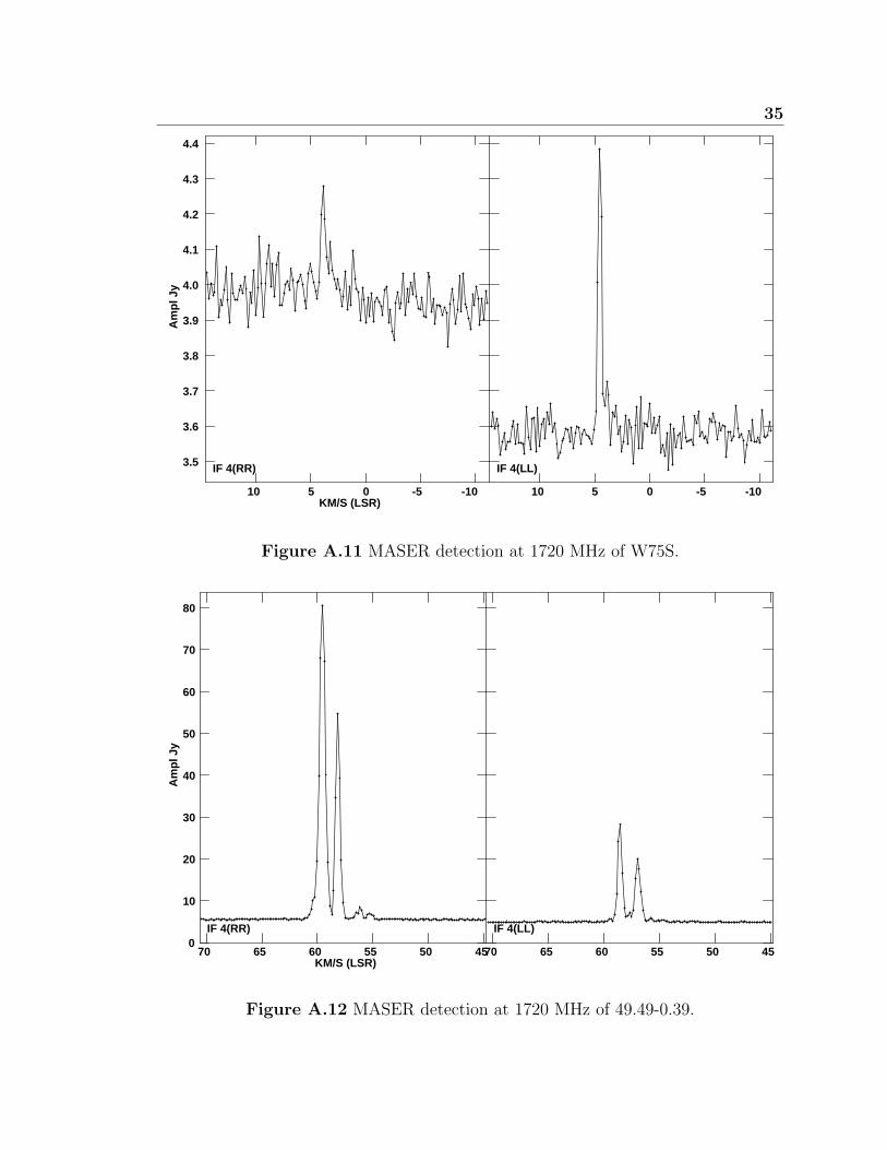
The high-mass SFR source 49.49-0.39 had 1720 MHz emission 35, 24, and 6.0
Janskys above the noise Fig. A.12.

18
Am
pl J
y
KM/S (LSR)-35 -40 -45 -50 -55
9
8
7
6
5
4
IF 4(RR)
Figure 3.4 MASER detection 1720 MHz W3OH in RR polarization.
The high-mass SFR source 35.20-1.73 had 1720 MHz emission 1 Jansky above the
noise Fig. A.8.
The high-mass SFR source W75N had 1720 MHz emission 1.0 and 0.23 Janskys
above the noise Fig. A.10.
The high-mass SFR source W75S had 1720 MHz emission 0.35 Janskys above the
noise Fig. A.11.
The source 30.60-0.06 had 1612 MHz emission 0.4 Janskys above the noise Fig.
A.6.It is not known whether this is a high-mass or low-mass SFR.
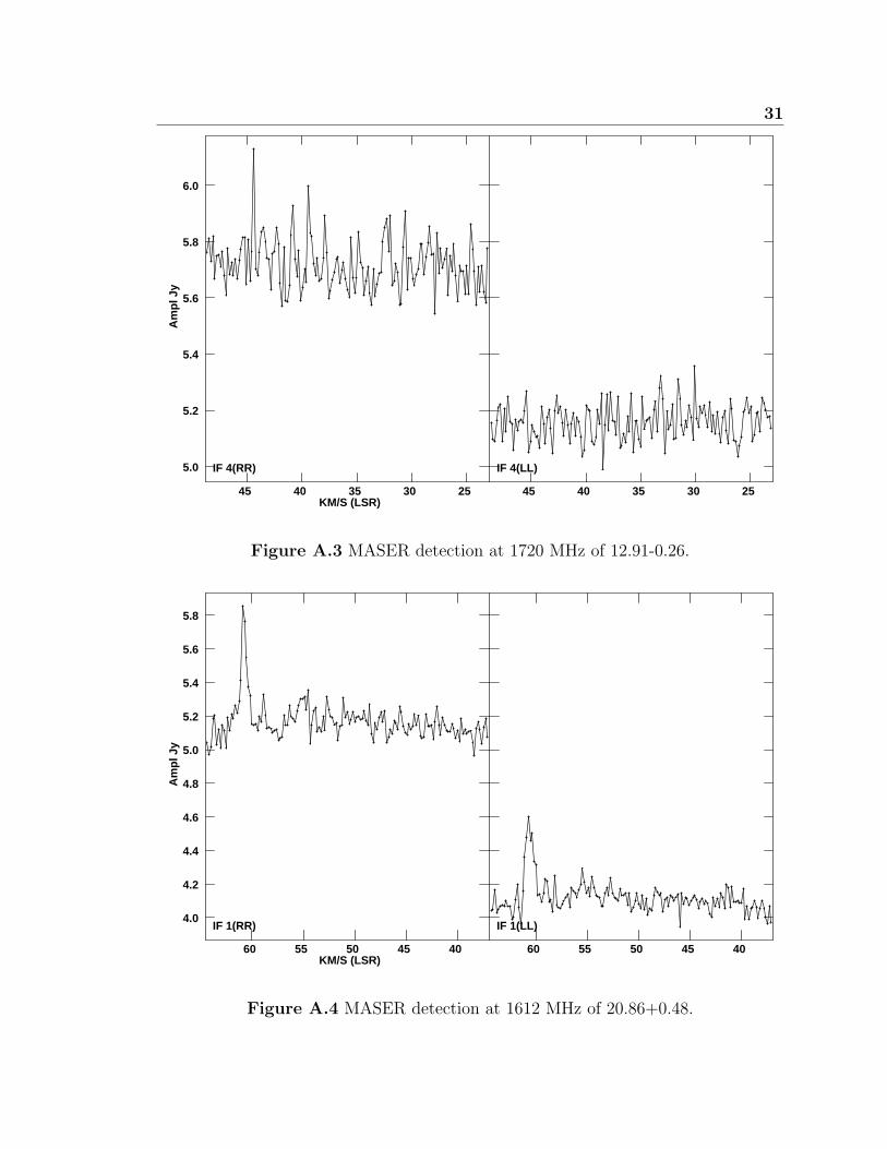
The source 20.86+0.48 had 1612 MHz emission 0.6 Janskys above the noise Fig.
A.4.It is not known whether this is a high-mass or low-mass SFR.

19
The source 12.22-0.12 had 1612 MHz emission 0.25 Janskys above the noise Fig.
A.1. It is not known whether this is a high-mass or low-mass SFR.
The source 28.87+0.06 had 1720 MHz emission 0.5 Janskys above the noise Fig.
A.5.It is not known whether this is a high-mass or low-mass SFR.
The source 12.68-0.18 had 1720 MHz emission 0.49 Janskys above the noise Fig.
A.2.It is not known whether this is a high-mass or low-mass SFR.
The source 31.29+0.06 had 1720 MHz emission 0.3 Janskys above the noise Fig.
A.7.It is not known whether this is a high-mass or low-mass SFR.
The source 12.91-0.26 had 1720 MHz emission 0.1 Janskys above the noise Fig.
A.3.It is not known whether this is a high-mass or low-mass SFR.

20
Am
pl J
y
KM/S (LSR)-30 -35 -40 -45 -50 -55
17
16
15
14
13
12
11
10IF 1(I)
Figure 3.5 MASER detection at 1612 MHz of W3OH. The horizontal axisis the LSR velocity. The vertical axis is in Janskys a unit of intensity
Am
pl J
y
KM/S (LSR)-35 -40 -45 -50 -55
5.5
5.0
4.5
4.0
3.5
3.0
2.5 IF 4(I)
Figure 3.6 MASER detection 1720 MHz W3OH.

21
Table 3.1 Summary of detections of the strongest OH-MASER emission forthe given sources. The common source names and IRAS names are givenwith galactic coordinates and RA and Dec and VLSR. The symbol † meansno detection.
Galactic Common R.A. DEC VLSR Frequency (MHZ) Mass
IRAS Name Coordinates Name (J2000) (J2000) (km/s) 1612 1720 H/L
02232+6138 133.90+1.10 W3(OH) 02 27 04.1 + 61 52 22 -44.3 6.0 Jy 3.0 Jy high
21413+5442 98.04+1.45 21 43 00.9 + 54 56 19 -61.0 0.2 Jy † high
23116+6111 111.54+0.78 NGC 7538 23 13 45.3 + 61 28 10 -57.4 † 8.5 Jy high
49.49-0.39 W51 19 23 43.9 + 14 30 27 57.0 † 35.0 Jy high
18895+0108 35.20-1.73 W48 19 01 45.5 + 01 13 32 32.1 † 1.0 Jy high
81.87+.078 W75N 20 38 37.5 + 42 37 54 7.0 † 1.0 Jy high
81.72+0.57 W75S 20 39 00.9 + 42 22 48 1.0 † 0.35 Jy high
18075-1956 10.62-0.38 W31 18 10 28.6 - 19 55 51 -2.2 † † high
18507+0110 34.26+0.15 18 53 18.7 + 01 14 59 58.0 † † high
22543+6145 109.87+2.11 CEPA 22 56 18 + 62 01 50 -13.8 † † high
22176+6303 106.80+5.31 S 140 22 19 18.4 + 63 18 45 -8.2 † † high
21381+5000 94.60-1.81 GL2789 21 40 00.8 + 50 13 39 -41.0 † † high
18018-2426 6.05-1.45 CRL2059 18 04 53.9 - 24 26 41 11.0 † † low
18265-1517 16.87-2.16 L379 18 29 24.5 - 15 15 15 16.0 † † low
18273+0113 31.58+5.38 SERPENS 18 29 49.7 + 01 15 20 9.5 † † low
20275+4001 78.89+0.71 AFGL2591 20 29 24.9 + 40 11 21 -8.8 † † low
00338+6312 121.30+0.66 L1287 00 36 47.5 + 63 29 02 -22.8 † † low
05137+3919 168.06+0.82 0513+393 05 17 13.3 + 39 22 14 -21.0 † † low
05168+3634 170.66-0.27 0516+365 05 20 16.1 + 36 37 21 -16.0 † † low
06117+1350 196.45-1.68 S269 06 14 37.3 + 13 49 36 16.0 † † low
20.86+0.48 18 27 25.9 - 10 30 24 50.0 0.6 Jy † n/a
03060-0004 30.60-0.06 18 47 19.9 - 02 05 57 37.5 0.4 Jy † n/a
01222-0012 12.22-0.12 18 12 44.5 - 18 24 25 27.0 0.25 Jy † n/a
02886+0007 28.87+0.06 18 43 48.1 - 03 35 31 103.0 † 0.5 Jy n/a
12.68-0.18 W33B 18 13 54.7 - 18 01 46 61.5 † 0.49 Jy n/a
03129+0007 31.29+0.06 18 48 45.2 - 01 33 12 107.5 † 0.3 Jy n/a
18117-1753 12.91-0.26 18 14 39.5 - 17 52 00 35.2 † 0.1 Jy n/a

22
Table 3.2 Galactic OH-MASER sources with no detections. The commonsource names are given with coordinates and V LSR. The symbol † meansno detection.
Galactic Common R.A. DEC VLSR Frequency (MHZ) Mass
IRAS Name Coordinates Name (J2000) (J2000) (km/s) 1612 1720 H/L
03274-0008 32.74-0.07 18 51 21.5 - 00 12 11 32.3 † † n/a
17574-2403 5.88-0.39 18 00 34.4 -24 04 04 14.0 † † n/a
18032-2032 9.62+0.20 18 06 14.7 - 20 31 31 1.8 † † n/a
01190-0014 11.91-0.15 18 12 11.3 -18 41 30 40.5 † † n/a
01289+0049 12.89+0.49 18 11 51.3 - 17 31 29 35.0 † † n/a
01961-0023 19.61-0.23 18 27 38 - 11 56 36 42.0 † † n/a
02008-0013 20.08-0.13 18 28 10 - 11 28 50 46.5 † † n/a
03124-0011 31.24-0.11 18 48 12.4 -01 25 48 21.2 † † n/a
03140-0026 31.40-0.26 18 49 33 - 01 29 04 85.0 † † n/a
03313-0009 33.13-0.09 18 52 07.3 + 00 08 06 78.5 † † n/a
03558-0003 35.58-0.03 18 56 22.5 + 02 20 27 48.9 † † n/a
21306+5539 97.52+3.18 21 32 11.3 + 55 53 30 -66.5 † † n/a
20350+5126 80.87+0.42 W70 20 36 52.6 +41 36 52.6 -8.0 † † n/a
20126+4104 78.12+3.63 20 14 26 + 41 13 32 -4.0 † † n/a

23
Table 3.3 Galactic OH-MASER sources with detections. The commonsource names are given with coordinates and V LSR. The symbol † meansno detection.
IRAS Galactic Common R.A. DEC 1612 1720 Mass
01222-0012 12.22-0.12 18 12 44.5 - 18 24 25 LL †
12.68-0.18 W33B 18 13 54.7 - 18 01 46 † RR
18117-1753 12.91-0.26 18 14 39.5 - 17 52 00 † RR
20.86+0.48 18 27 25.9 - 10 30 24 RR/LL †
02886+0007 28.87+0.06 18 43 48.1 - 03 35 31 † RR/LL
03060-0004 30.60-0.06 18 47 19.9 - 02 05 57 LL †
03129+0007 31.29+0.06 18 48 45.2 - 01 33 12 † RR/LL
18895+0108 35.20-1.73 W48 19 01 45.5 + 01 13 32 † RR/LL H
21413+5442 98.04+1.45 21 43 00.9 + 54 56 19 RR/LL † H
81.87+.078 W75N 20 38 37.5 + 42 37 54 † RR/LL H
81.72+0.57 W75S 20 39 00.9 + 42 22 48 † RR/LL H
49.49-0.39 W51 19 23 43.9 + 14 30 27 † RR*2/LL*2 H
02232+6138 133.90+1.10 W3(OH) 02 27 04.1 + 61 52 22 RR/LL RR*2/LL*2 H
23116+6111 111.54+0.78 NGC 7538 23 13 45.3 + 61 28 10 † RR*2/LL H

Chapter 4
Discussion
The intensity of the MASER emission and the resolution of our instruments allowed
us to detect many OH-MASERs and resolve many multi-peaked spectra Fig. A.9.
Seven of the twelve known high-mass SFR showed 1612 or 1720 MHz emission. Seven
regions with detections are not determined as high-mass or low-mass. None of the
eight low-mass SFR show 1612 or 1720 MHz emission. That leaves the other 14 sources
having no detection and an unknown mass classification. Having only satellite line
emission occur in high-mass SFR of the 20 known high-mass/low-mass SFR shows us
there is a correlation.
From the data we obtained spectra that we summarized in Table 3.1. The known
high-mass SFR regions have strong MASER emission the unknown SFR that have
emission are very weak, and the known low-mass SFR have none detected. This
may be the greatest understanding we pull from this OH satellite line survey of SFR.
Satellite line detection in high-mass SFR may correlate with line strength. Seeing
this line strength can depend on the signal to noise ratio we obtain.
24

4.1 Future Study 25
Caswell [4] reported 1720 MHz masers are 1/6 as common as 1665 MHz in the
southern sky. It is very rare to find a 1720 MHz detection without a 1665 MHz
detection. Caswell explains that this could be because only 1720 emission is above
the threshold limit. Since our instruments have a limitation on detecting MASER
emission we may only see the appearance of satellite lines where they are strong and
intense. The strength of the signal depends on the signal to noise ratio proportional
to√t. We only observed each source for five minutes which doesn’t produce a high
signal to noise ratio. Because of short integration (observing) times we were limited
to make good maps with great UV coverage.
4.1 Future Study
A study of these sources at similar resolution with longer integration time will
provide more evidence for our assumption that the satellite lines only appear in SFR.
Being able to observe these sources we studied in this survey for longer integration
times will yield a higher signal to noise ratio and will most likely yield the appearance
of more satellite lines being detected in these regions. Perhaps with equipment that
has enough resolution and sensitivity we may discover that the MASER emission
strength is directly related to the mass of nearby proto-stars. The exact cause of
how MASER conditions are reached in SFR is unknown and can be studied further
through detecting MASER emission with high signal to noise ratios.
Chapter 5
Conclusions
We learned the effectiveness of interferometry techniques that can be used to achieve
very high spatial resolution. We learned data reduction procedures in AIPS along
with debugging calibration problems, strategies to reduce many sources at once, and
applying tables to data. These reductions help us understand the conditions that
are occurring in SFR. Caswell [4] noted 1720 MHz emission requires higher density,
which is true of high-mass vs. low-mass SFR. We need to consider how large that
gap is, and does it mean that low-mass SFR are not dense enough to have 1720 MHz
emission.
The OH-MASER 1720 MHz line correlates with high-mass SFR. The 1612 MHz
line showed a weaker correlation but still, as in the case of the 1720 MHz line, only
appeared in sources that are not previously known as low-mass SFR. From this we
learn that the OH satellites are a useful tool in describing and identifying high-mass
SFR. We understand that high-mass SFR contain different physical conditions that
allow for stronger MASER emission of the OH satellite lines.
26

Bibliography
[1] F. H. Shu, F. C. Adams, and S. Lizano, “Star formation in molecular clouds -
Observation and theory,” ARAA .
[2] J. L. Caswell, “Star formation: relationship between the maser species,” In Cos-
mic Masers: From Proto-Stars to Black Holes, V. Migenes & M. J. Reid, ed.,
IAU Symposium 206, 1–+ (2002).
[3] V. L. Fish and M. J. Reid, “Full-Polarization Observations of OH Masers in
Massive Star-forming Regions. II. Maser Properties and the Interpretation of
Polarization,” ApJs 164, 99–123 (2006).
[4] J. L. Caswell, “OH 1720-MHz masers in southern star-forming regions,” MNRAS
349, 99–114 (2004).
[5] M. J. Reid, A. D. Haschick, B. F. Burke, J. M. Moran, K. J. Johnston, and G. W.
Swenson, Jr., “The structure of interstellar hydroxyl masers - VLBI synthesis
observations of W3/OH/,” ApJ 239, 89–99 (1980).
[6] A. D. Haschick, M. J. Reid, B. F. Burke, J. M. Moran, and G. Miller, “VLBI
aperture synthesis observations of the OH maser source W75 N,” ApJ 244, 76–87
(1981).
27

BIBLIOGRAPHY 28
[7] X. Zheng, “VLBI observation of OH masers in G 45.07+0.13,” Chinese Astron-
omy and Astrophysics 21, 182–190 (1997).
[8] V. I. Slysh et al., “Space-VLBI observations of the OH maser OH34.26+0.15:
low interstellar scattering,” MNRAS 320, 217–223 (2001).
[9] V. I. Slysh, V. Migenes, I. E. Val’tts, S. Y. Lyubchenko, S. Horiuchi, V. I.
Altunin, E. B. Fomalont, and M. Inoue, “Total Linear Polarization in the OH
Maser W75 N: VLBA Polarization Structure,” ApJ 564, 317–326 (2002).
[10] M. J. M. Thompson, A. R. and J. Swenson, Interferometry & Synthesis in Radio
Astronomy (2001).
[11] R. E. Spencer, “Fundamentals of interferometry.,” In Techniques and Applica-
tions of Very Long Baseline Interferometry, pp. 11–25 (1989).
[12] B. Anderson, “Basic radio astronomy.,” In Techniques and Applications of Very
Long Baseline Interferometry, pp. 3–10 (1989).

Appendix A
The list of plots of MASER
emission
29

30
IF 1(RR)
Am
pl J
y
KM/S (LSR)40 35 30 25 20 15
5.4
5.2
5.0
4.8
4.6
4.4
IF 1(LL)
40 35 30 25 20 15
Figure A.1 MASER detection at 1612 MHz of 12.22-0.12.
IF 4(RR)
Am
pl J
y
KM/S (LSR)75 70 65 60 55 50
5.9
5.8
5.7
5.6
5.5
5.4
5.3
5.2
5.1 IF 4(LL)
75 70 65 60 55 50
Figure A.2 MASER detection at 1720 MHz of 12.68-0.18.
31
IF 4(RR)
Am
pl J
y
KM/S (LSR)45 40 35 30 25
6.0
5.8
5.6
5.4
5.2
5.0 IF 4(LL)
45 40 35 30 25
Figure A.3 MASER detection at 1720 MHz of 12.91-0.26.
IF 1(RR)
Am
pl J
y
KM/S (LSR)60 55 50 45 40
5.8
5.6
5.4
5.2
5.0
4.8
4.6
4.4
4.2
4.0IF 1(LL)
60 55 50 45 40
Figure A.4 MASER detection at 1612 MHz of 20.86+0.48.

32
IF 4(RR)
Am
pl J
y
KM/S (LSR)115 110 105 100 95
5.2
5.0
4.8
4.6
4.4
4.2
4.0
IF 4(LL)
115 110 105 100 95
Figure A.5 MASER detection at 1720 MHz of 28.87+0.06.
IF 1(RR)
Am
pl J
y
KM/S (LSR)50 45 40 35 30 25
5.6
5.4
5.2
5.0
4.8
4.6
4.4 IF 1(LL)
50 45 40 35 30 25
Figure A.6 MASER detection at 1612 MHz of 30.60-0.06.

33
IF 4(RR)
Am
pl J
y
KM/S (LSR)120 115 110 105 100
5.2
5.0
4.8
4.6
4.4
4.2
4.0
IF 4(LL)
120 115 110 105 100
Figure A.7 MASER detection at 1720 MHz of 31.29+0.06.
IF 4(RR)
Am
pl J
y
KM/S (LSR)45 40 35 30 25 20
5.2
5.0
4.8
4.6
4.4
4.2
4.0
3.8
3.6IF 4(LL)
45 40 35 30 25 20
Figure A.8 MASER detection at 1720 MHz of 35.20-1.73.

34
IF 1(RR)
Am
pl J
y
KM/S (LSR)-50 -55 -60 -65 -70
4.8
4.6
4.4
4.2
4.0
3.8
3.6
3.4
IF 1(LL)
-50 -55 -60 -65 -70
Figure A.9 MASER detection at 1612 MHz of 98.04+1.45.
IF 4(RR)
Am
pl J
y
KM/S (LSR)20 15 10 5 0 -5
6.0
5.5
5.0
4.5
4.0
3.5
IF 4(LL)
20 15 10 5 0 -5
Figure A.10 MASER detection at 1720 MHz of W75N.
35
IF 4(RR)
Am
pl J
y
KM/S (LSR)10 5 0 -5 -10
4.4
4.3
4.2
4.1
4.0
3.9
3.8
3.7
3.6
3.5 IF 4(LL)
10 5 0 -5 -10
Figure A.11 MASER detection at 1720 MHz of W75S.
IF 4(RR)
Am
pl J
y
KM/S (LSR)70 65 60 55 50 45
80
70
60
50
40
30
20
10
0IF 4(LL)
70 65 60 55 50 45
Figure A.12 MASER detection at 1720 MHz of 49.49-0.39.

36
IF 1(RR)
Am
pl J
y
KM/S (LSR)-30 -35 -40 -45 -50 -55
30
25
20
15
10
5
0IF 1(LL)
-30 -35 -40 -45 -50 -55
Figure A.13 MASER detection at 1612 MHz of W3OH.
IF 4(RR)
Am
pl J
y
KM/S (LSR)-35 -40 -45 -50 -55
11
10
9
8
7
6
5
4
3IF 4(LL)
-35 -40 -45 -50 -55
Figure A.14 MASER detection at 1720 MHz of W3OH.

37
IF 4(RR)
Am
pl J
y
KM/S (LSR)-45 -50 -55 -60 -65
20
15
10
5
0IF 4(LL)
-45 -50 -55 -60 -65
Figure A.15 MASER detection at 1720 MHz of NGC 7538.


![Unit 4: Mechanical Report 4 - Mechanical...[UNIT 4: MECHANICAL REPORT] Jason Brognano, Michael Gilroy, Stephen Kijak, David Maser 4-28 KGB Maser| IPD/BIM Thesis | PSU Millennium Science](https://img.pdfslide.us/doc/110x75/5ed10d203603e925722bf535/unit-4-mechanical-report-4-mechanical-unit-4-mechanical-report-jason-brognano.jpg)