The Design and Evaluation of Network Power Scheduling for Sensor Networks

by

Barbara Ann Hohlt

M.S. (University of California, Berkeley) 2001

A dissertation submitted in partial satisfactionof the requirements for the degree of

Doctor of Philosophy

in

Computer Science

in the

GRADUATE DIVISION

of the

UNIVERSITY OF CALIFORNIA, BERKELEY

Committee in charge:

Professor Eric A. Brewer, ChairProfessor David E. CullerProfessor Paul K. Wright

Spring 2005

The Design and Evaluation of Network Power Scheduling for Sensor Networks

Copyright 2005

by

Barbara Ann Hohlt

1

ABSTRACT

The Design and Evaluation of Network Power Scheduling for Sensor Networks

by

Barbara Ann Hohlt

Doctor of Philosophy in Computer Science

University of California, Berkeley

Professor Eric A. Brewer, Chair

The combination of technological advances in integrated circuitry, micro-electro-

mechanical systems, communication, and energy storage has driven the development of

low-cost, low-power sensor nodes. Networking many nodes through radio communication

allows for data collection via multihop routing, but the practical limits on available

resources and the lack of global control present challenges. Constraints imposed by the

limited energy stores on individual nodes require planned use of resources, particularly the

radio.

In this dissertation we present Flexible Power Scheduling (FPS), a network scheduling

architecture for radio power management specifically tailored towards energy-efficient

data gathering and query dissemination in multihop sensor networks. We present empiri-

cal results from experiments on Berkeley Motes running two real-world sensor network

applications and show that FPS increases end-to-end packet reception and decreases

power consumption by 4X over existing power management approaches.

ACKNOWLEDGEMENTS

Eric Brewer is my advisor and mentor. He is the best advisor I could have hoped for

and I cannot envision this journey without him. I thank him for the advice, guidance, cri-

tique, and insights he has shared with me over the years.

I am much indebted to Rob Szewczyk for his continuous help, support, and advice on

the topics of power management and TinyOS. We spent many happy hours debugging

code, running experiments, and discussing the fascinating topic of sensor networks.

Lance Doherty contributed significantly to early versions of the ideas presented on

power scheduling and was co-author on the first published paper. I am honored to have

had the opportunity to work with him.

Thanks goes to Kris Pister and Jason Hill who pioneered the SmartDust and TinyOS

research and to David Culler who made it a revolution. I thank David also for his helpful

comments and feedback on this dissertation.

Paul Wright has been an unfailing source of support and inspiration throughout my

dissertation. Paul introduced me to the wonderful world of motes and generously served

on both my qualifying and dissertation committees, encouraging me every step of the way.

I am fortunate to have had the guidance and support of many faculty at Berkeley, espe-

cially Randy Katz, Anthony Joseph, Alan Smith, and Shankar Sastry. Thank you for the

opportunities you have opened for me.

To my dear friends Keith Stattenfield and Loretta Beavers. Thank you for getting me

here and keeping the faith.

i

Finally, I am especially grateful to my family — Mom, Dad, Randy, Mary K., Clyde,

Katherine, Elizabeth, Joan and Roger. This would not have been possible without your

love and support.

ii

Contents

List of Figures viii

List of Tables xi

1 Introduction 1

1.1 Power and Sensor Networks . . . . . . . . . . . . . . . . . . . . . . . . . . . . . . . . . . . . . . . . . . 1

1.2 The Network Scheduling Approach . . . . . . . . . . . . . . . . . . . . . . . . . . . . . . . . . . . . 3

1.3 Contributions . . . . . . . . . . . . . . . . . . . . . . . . . . . . . . . . . . . . . . . . . . . . . . . . . . . . . 6

1.4 Additional Contributions . . . . . . . . . . . . . . . . . . . . . . . . . . . . . . . . . . . . . . . . . . . . 7

1.5 Six Design Principles . . . . . . . . . . . . . . . . . . . . . . . . . . . . . . . . . . . . . . . . . . . . . . . 8

1.6 Summary . . . . . . . . . . . . . . . . . . . . . . . . . . . . . . . . . . . . . . . . . . . . . . . . . . . . . . . . 12

2 Background 13

2.1 Power Consumption and Communication . . . . . . . . . . . . . . . . . . . . . . . . . . . . . . 13

2.2 Multihop Sensor Networks . . . . . . . . . . . . . . . . . . . . . . . . . . . . . . . . . . . . . . . . . . 15

2.3 Time Division Multiplexing . . . . . . . . . . . . . . . . . . . . . . . . . . . . . . . . . . . . . . . . . 17

2.4 Two-level Architecture . . . . . . . . . . . . . . . . . . . . . . . . . . . . . . . . . . . . . . . . . . . . . 19

2.5 Time Synchronization. . . . . . . . . . . . . . . . . . . . . . . . . . . . . . . . . . . . . . . . . . . . . . 20

2.6 Other Related Work . . . . . . . . . . . . . . . . . . . . . . . . . . . . . . . . . . . . . . . . . . . . . . . 22

iii

3 Adaptive Communication Scheduling 26

3.1 FPS Protocol . . . . . . . . . . . . . . . . . . . . . . . . . . . . . . . . . . . . . . . . . . . . . . . . . . . . . 26

3.1.1 Goals . . . . . . . . . . . . . . . . . . . . . . . . . . . . . . . . . . . . . . . . . . . . . . . . . . . . . . 26

3.1.2 Assumptions . . . . . . . . . . . . . . . . . . . . . . . . . . . . . . . . . . . . . . . . . . . . . . . . 27

3.1.3 Power Scheduling . . . . . . . . . . . . . . . . . . . . . . . . . . . . . . . . . . . . . . . . . . . . 27

3.2 Supply and Demand . . . . . . . . . . . . . . . . . . . . . . . . . . . . . . . . . . . . . . . . . . . . . . . 29

3.2.1 Scheduling Flows . . . . . . . . . . . . . . . . . . . . . . . . . . . . . . . . . . . . . . . . . . . . 29

3.2.2 Flow Preallocation . . . . . . . . . . . . . . . . . . . . . . . . . . . . . . . . . . . . . . . . . . . 31

3.3 A Walk Through . . . . . . . . . . . . . . . . . . . . . . . . . . . . . . . . . . . . . . . . . . . . . . . . . 33

3.3.1 Formulation . . . . . . . . . . . . . . . . . . . . . . . . . . . . . . . . . . . . . . . . . . . . . . . . 33

3.3.2 A Simple Example . . . . . . . . . . . . . . . . . . . . . . . . . . . . . . . . . . . . . . . . . . . 34

3.4 Algorithm Details . . . . . . . . . . . . . . . . . . . . . . . . . . . . . . . . . . . . . . . . . . . . . . . . 35

3.4.1 Maintaining Node States and Schedules. . . . . . . . . . . . . . . . . . . . . . . . . . . 35

3.4.2 Partial Flows and Communication Broadcast I . . . . . . . . . . . . . . . . . . . . . 36

3.4.3 State Diagram for FPS Protocol . . . . . . . . . . . . . . . . . . . . . . . . . . . . . . . . . 37

3.4.4 Main Operation. . . . . . . . . . . . . . . . . . . . . . . . . . . . . . . . . . . . . . . . . . . . . . 39

3.4.5 Making Reservations . . . . . . . . . . . . . . . . . . . . . . . . . . . . . . . . . . . . . . . . . 40

3.4.6 Canceling Reservations . . . . . . . . . . . . . . . . . . . . . . . . . . . . . . . . . . . . . . . 41

3.5 Special Cases . . . . . . . . . . . . . . . . . . . . . . . . . . . . . . . . . . . . . . . . . . . . . . . . . . . . 42

3.5.1 Joining the Network . . . . . . . . . . . . . . . . . . . . . . . . . . . . . . . . . . . . . . . . . . 42

3.5.2 Initialization and Ripple Advertisements . . . . . . . . . . . . . . . . . . . . . . . . . . 43

3.5.3 Adaptive Advertisements . . . . . . . . . . . . . . . . . . . . . . . . . . . . . . . . . . . . . . 44

3.6 Other Considerations . . . . . . . . . . . . . . . . . . . . . . . . . . . . . . . . . . . . . . . . . . . . . . 45

iv

3.6.1 Collisions and Message Loss . . . . . . . . . . . . . . . . . . . . . . . . . . . . . . . . . . . 45

3.6.2 Guard Times . . . . . . . . . . . . . . . . . . . . . . . . . . . . . . . . . . . . . . . . . . . . . . . . 46

3.6.3 Synchronization . . . . . . . . . . . . . . . . . . . . . . . . . . . . . . . . . . . . . . . . . . . . . 47

3.7 Summary . . . . . . . . . . . . . . . . . . . . . . . . . . . . . . . . . . . . . . . . . . . . . . . . . . . . . . . . 49

4 Adapting to Demand 50

4.1 Mica Experiment Setup . . . . . . . . . . . . . . . . . . . . . . . . . . . . . . . . . . . . . . . . . . . . 51

4.2 Network Adaptation . . . . . . . . . . . . . . . . . . . . . . . . . . . . . . . . . . . . . . . . . . . . . . . 51

4.3 Response Time . . . . . . . . . . . . . . . . . . . . . . . . . . . . . . . . . . . . . . . . . . . . . . . . . . . 54

4.4 Fault Tolerance . . . . . . . . . . . . . . . . . . . . . . . . . . . . . . . . . . . . . . . . . . . . . . . . . . . 55

4.4.1 Parent and Child Failures . . . . . . . . . . . . . . . . . . . . . . . . . . . . . . . . . . . . . . 55

4.4.2 Network Stability . . . . . . . . . . . . . . . . . . . . . . . . . . . . . . . . . . . . . . . . . . . . 57

4.5 Fractional Flows . . . . . . . . . . . . . . . . . . . . . . . . . . . . . . . . . . . . . . . . . . . . . . . . . . 58

5 Network 61

5.1 Measured Current and Duty Cycle . . . . . . . . . . . . . . . . . . . . . . . . . . . . . . . . . . . . 61

5.2 Scheduled vs Unscheduled . . . . . . . . . . . . . . . . . . . . . . . . . . . . . . . . . . . . . . . . . . 65

5.2.1 Contention . . . . . . . . . . . . . . . . . . . . . . . . . . . . . . . . . . . . . . . . . . . . . . . . . 66

5.2.2 Fairness and Throughput . . . . . . . . . . . . . . . . . . . . . . . . . . . . . . . . . . . . . . 69

5.3 Duty Cycle and Latency . . . . . . . . . . . . . . . . . . . . . . . . . . . . . . . . . . . . . . . . . . . . 71

5.4 Optimized Latency Scheduling. . . . . . . . . . . . . . . . . . . . . . . . . . . . . . . . . . . . . . . 73

5.4.1 Reservation Window . . . . . . . . . . . . . . . . . . . . . . . . . . . . . . . . . . . . . . . . . 74

5.4.2 Fractional Flows . . . . . . . . . . . . . . . . . . . . . . . . . . . . . . . . . . . . . . . . . . . . . 75

5.5 Partial Flows and Broadcast II . . . . . . . . . . . . . . . . . . . . . . . . . . . . . . . . . . . . . . . 76

v

6 Application: Great Duck Island 78

6.1 Great Duck Island . . . . . . . . . . . . . . . . . . . . . . . . . . . . . . . . . . . . . . . . . . . . . . . . . 78

6.2 GDI with Low-Power Listening . . . . . . . . . . . . . . . . . . . . . . . . . . . . . . . . . . . . . . 79

6.3 GDI with FPS . . . . . . . . . . . . . . . . . . . . . . . . . . . . . . . . . . . . . . . . . . . . . . . . . . . . 80

6.4 Experimental Setup. . . . . . . . . . . . . . . . . . . . . . . . . . . . . . . . . . . . . . . . . . . . . . . . 81

6.5 Measuring Current . . . . . . . . . . . . . . . . . . . . . . . . . . . . . . . . . . . . . . . . . . . . . . . . 82

6.6 Evaluation . . . . . . . . . . . . . . . . . . . . . . . . . . . . . . . . . . . . . . . . . . . . . . . . . . . . . . . 83

6.6.1 Power Comparison with Low-Power Listening . . . . . . . . . . . . . . . . . . . . . 83

6.6.2 Yield and Fairness . . . . . . . . . . . . . . . . . . . . . . . . . . . . . . . . . . . . . . . . . . . 87

6.6.3 Comparison with GDI Deployment . . . . . . . . . . . . . . . . . . . . . . . . . . . . . . 88

7 Application: TinyDB 90

7.1 TinyDB . . . . . . . . . . . . . . . . . . . . . . . . . . . . . . . . . . . . . . . . . . . . . . . . . . . . . . . . . 91

7.2 Estimating Power Consumption . . . . . . . . . . . . . . . . . . . . . . . . . . . . . . . . . . . . . . 92

7.3 The Redwood Deployment . . . . . . . . . . . . . . . . . . . . . . . . . . . . . . . . . . . . . . . . . . 93

7.4 TinyDB with Duty Cycling. . . . . . . . . . . . . . . . . . . . . . . . . . . . . . . . . . . . . . . . . . 94

7.5 TinyDB with FPS . . . . . . . . . . . . . . . . . . . . . . . . . . . . . . . . . . . . . . . . . . . . . . . . . 95

7.6 FPS Validation . . . . . . . . . . . . . . . . . . . . . . . . . . . . . . . . . . . . . . . . . . . . . . . . . . . 97

7.7 Power Savings. . . . . . . . . . . . . . . . . . . . . . . . . . . . . . . . . . . . . . . . . . . . . . . . . . . . 99

8 Advanced Techniques 103

8.1 Forwarding Queues. . . . . . . . . . . . . . . . . . . . . . . . . . . . . . . . . . . . . . . . . . . . . . . 103

8.2 Global Buffer Management . . . . . . . . . . . . . . . . . . . . . . . . . . . . . . . . . . . . . . . . 105

8.2.1 Application Bufffer Allocation. . . . . . . . . . . . . . . . . . . . . . . . . . . . . . . . . 106

8.2.2 Network Buffer Swapping . . . . . . . . . . . . . . . . . . . . . . . . . . . . . . . . . . . . 106

vi

8.2.3 Determining Free Lists . . . . . . . . . . . . . . . . . . . . . . . . . . . . . . . . . . . . . . . 107

8.2.4 Message Processing . . . . . . . . . . . . . . . . . . . . . . . . . . . . . . . . . . . . . . . . . 108

8.3 Pseudo-random Number Generation . . . . . . . . . . . . . . . . . . . . . . . . . . . . . . . . . 109

9 Future Work 110

9.1 Power-aware Multihop Routing . . . . . . . . . . . . . . . . . . . . . . . . . . . . . . . . . . . . . 110

9.2 Network Load Balancing . . . . . . . . . . . . . . . . . . . . . . . . . . . . . . . . . . . . . . . . . . 111

9.3 Optimized Scheduling. . . . . . . . . . . . . . . . . . . . . . . . . . . . . . . . . . . . . . . . . . . . . 112

9.4 Buffer Management . . . . . . . . . . . . . . . . . . . . . . . . . . . . . . . . . . . . . . . . . . . . . . 112

9.5 Summary . . . . . . . . . . . . . . . . . . . . . . . . . . . . . . . . . . . . . . . . . . . . . . . . . . . . . . . 113

10 Concluding Remarks 114

Bibliography 116

vii

List of Figures

Figure 3-1: Slots and Cycles . . . . . . . . . . . . . . . . . . . . . . . . . . . . . . . . . . . . . . . . . . . 28

Figure 3-2: A Local Power Schedule . . . . . . . . . . . . . . . . . . . . . . . . . . . . . . . . . . . . 28

Figure 3-3: Data Traffic State Machine . . . . . . . . . . . . . . . . . . . . . . . . . . . . . . . . . . 29

Figure 3-4: Supply and Demand State Machine . . . . . . . . . . . . . . . . . . . . . . . . . . . . 31

Figure 3-5: K Cycles of a Power Schedule. . . . . . . . . . . . . . . . . . . . . . . . . . . . . . . . 33

Figure 3-6: Demand Example. . . . . . . . . . . . . . . . . . . . . . . . . . . . . . . . . . . . . . . . . . 35

Figure 3-7: FPS State Diagram. . . . . . . . . . . . . . . . . . . . . . . . . . . . . . . . . . . . . . . . . 38

Figure 4-1: Network Topology and Demand . . . . . . . . . . . . . . . . . . . . . . . . . . . . . . 52

Figure 4-2: Network Adaptation. . . . . . . . . . . . . . . . . . . . . . . . . . . . . . . . . . . . . . . . 52

Figure 4-3: Response Time. . . . . . . . . . . . . . . . . . . . . . . . . . . . . . . . . . . . . . . . . . . . 54

Figure 4-4: Fractional Flows. . . . . . . . . . . . . . . . . . . . . . . . . . . . . . . . . . . . . . . . . . . 59

Figure 5-1: Measured Current at an Intermediate Node . . . . . . . . . . . . . . . . . . . . . . 62

viii

Figure 5-2: Topology Used in Mica Indoor Experiments. . . . . . . . . . . . . . . . . . . . . 66

Figure 5-3: CDF of Backoff Counts . . . . . . . . . . . . . . . . . . . . . . . . . . . . . . . . . . . . . 68

Figure 5-4: Fairness and Yield . . . . . . . . . . . . . . . . . . . . . . . . . . . . . . . . . . . . . . . . . 70

Figure 5-5: 15-Node Binary Tree . . . . . . . . . . . . . . . . . . . . . . . . . . . . . . . . . . . . . . . 72

Figure 5-6: Duty Cycle vs Latency. . . . . . . . . . . . . . . . . . . . . . . . . . . . . . . . . . . . . . 72

Figure 5-7: Reservation Window . . . . . . . . . . . . . . . . . . . . . . . . . . . . . . . . . . . . . . . 75

Figure 6-1: 30 Second Sample Period . . . . . . . . . . . . . . . . . . . . . . . . . . . . . . . . . . . 85

Figure 6-2: 1 Minute Sample Period. . . . . . . . . . . . . . . . . . . . . . . . . . . . . . . . . . . . . 85

Figure 6-3: 5 Minute Sample Period. . . . . . . . . . . . . . . . . . . . . . . . . . . . . . . . . . . . . 86

Figure 6-4: 20 Minute Sample Period. . . . . . . . . . . . . . . . . . . . . . . . . . . . . . . . . . . . 86

Figure 7-1: Sub-tree Redwood Deployment . . . . . . . . . . . . . . . . . . . . . . . . . . . . . . . 93

Figure 7-2: Topology with Demand for Estimates . . . . . . . . . . . . . . . . . . . . . . . . . . 95

Figure 7-3: Slot State and Radio State . . . . . . . . . . . . . . . . . . . . . . . . . . . . . . . . . . . 98

Figure 7-4: Mica Estimates (mA-seconds) . . . . . . . . . . . . . . . . . . . . . . . . . . . . . . . 100

Figure 7-5: Mica2 Estimate (mA-seconds). . . . . . . . . . . . . . . . . . . . . . . . . . . . . . . 101

Figure 8-1: Separating Policy from Mechanism. . . . . . . . . . . . . . . . . . . . . . . . . . . 104

Figure 8-2: Global Buffer Manager . . . . . . . . . . . . . . . . . . . . . . . . . . . . . . . . . . . . 105

ix

Figure 8-3: Application Buffer Allocation . . . . . . . . . . . . . . . . . . . . . . . . . . . . . . . 106

Figure 8-4: Network Buffer Swapping . . . . . . . . . . . . . . . . . . . . . . . . . . . . . . . . . . 107

Figure 8-5: Process Message Queue . . . . . . . . . . . . . . . . . . . . . . . . . . . . . . . . . . . . 108

Figure 9-1: Power-aware Multihop Routing. . . . . . . . . . . . . . . . . . . . . . . . . . . . . . 111

x

xi

List of Tables

Table 3-1: Slot States . . . . . . . . . . . . . . . . . . . . . . . . . . . . . . . . . . . . . . . . . . . . . . . . . 36

Table 3-2: Communication Operations . . . . . . . . . . . . . . . . . . . . . . . . . . . . . . . . . . . 37

Table 3-3: Making a Reservation. . . . . . . . . . . . . . . . . . . . . . . . . . . . . . . . . . . . . . . . 40

Table 3-4: Canceling a Reservation. . . . . . . . . . . . . . . . . . . . . . . . . . . . . . . . . . . . . . 41

Table 3-5: Joining . . . . . . . . . . . . . . . . . . . . . . . . . . . . . . . . . . . . . . . . . . . . . . . . . . . 42

Table 5-1: Calculation of Duty Cycle from Observed Schedules . . . . . . . . . . . . . . . 63

Table 5-2: Average Backoffs/Flow Delivered. . . . . . . . . . . . . . . . . . . . . . . . . . . . . . 67

Table 5-3: Average Backoffs/Flow Transmitted . . . . . . . . . . . . . . . . . . . . . . . . . . . . 68

Table 5-4: Throughput and Fairness . . . . . . . . . . . . . . . . . . . . . . . . . . . . . . . . . . . . . 71

Table 6-1: Power Measurement (mW) . . . . . . . . . . . . . . . . . . . . . . . . . . . . . . . . . . . 83

Table 6-2: Yield and Fairness Comparison . . . . . . . . . . . . . . . . . . . . . . . . . . . . . . . . 88

Table 6-3: Lab and Deployment Comparison . . . . . . . . . . . . . . . . . . . . . . . . . . . . . . 89

Table 7-1: Predicted vs. Measured Idle Time . . . . . . . . . . . . . . . . . . . . . . . . . . . . . . 97

Table 7-2: Power Consumption of Motes (mA) . . . . . . . . . . . . . . . . . . . . . . . . . . . . 99

Table 7-3: Radio-on Times (seconds per hour) . . . . . . . . . . . . . . . . . . . . . . . . . . . . . 99

Chapter 1

Introduction

The combination of technological advances in integrated circuitry, MEMS, communica-

tion and energy storage has driven the development of low-cost, low-power wireless sen-

sor nodes [Asad98, Kahn99]. Networking many nodes through radio communication

allows for data collection via multihop routing, but the practical limits on available power

and the lack of global control present challenges.

1.1 Power and Sensor Networks

Power is one of the dominant problems in wireless sensor networks today. Constraints

imposed by the limited energy stores on individual nodes require planned use of resources,

particularly the radio. Sensor network energy use tends to be particularly acute as deploy-

ments are left unattended for long periods of time, perhaps months or years.

Communication is the most costly task in terms of energy [Asad98, Dohe01, Sohr00,

Pott00]. At the communication distances typical in sensor networks, listening for informa-

tion on the radio channel costs about the same as data transmission [Ragh02]. Worse, the

1

energy cost for a node in idle mode is approximately the same as in receive mode. There-

fore, protocols that assume receive and idle power are of little consequence are not suit-

able for sensor networks. Idle listening, the time spent listening while waiting to receive

packets, is the most significant cost of radio communication. This is true for hand-held

devices [Stem97]. Thus, the biggest single action to save power is to turn the radio off dur-

ing idle times.

Turning the radio off implies advance knowledge that the radio will be idle. One

approach is to periodically duty-cycle nodes into wake and sleep periods [802.11,

SMAC02, DAM03, TinyDB]. The problem with duty-cycling schemes is they aim to syn-

chronize the network to transmit packets at the same or near-same time, which causes

severe packet loss in wireless multihop scenarios. In Section 5.2.1 we demonstrate the

severity of packet loss when transmiting packets over multiple hops at the same or near-

same time.

Another approach is preamble sampling (or low-power listening), in which nodes peri-

odically wake up their radios and check for activity on the channel [Mang95, ElHo02,

Hill02]. Packets are sent with long preambles to match the channel check period. These

techniques, however, require nodes to wake up any time communication is heard, regard-

less of whether the transmission is actually addressed to the local node, causing high

power consumption. Also, at low channel sampling rates in dense multihop networks,

these techniques have very low end-to-end packet reception due to the very long pream-

bles. We evaluate low-power listening and demonstrate these effects in Chapter 6.

An obvious approach is to use TDMA to turn the radio off at the MAC layer during

idle times. However, this requires tight time synchronization and typically hardware sup-

2

port. Also, because a TDMA must primarily solve for channel access, these approaches

by and large produce static global schedules that require centralized control and global

network phases to change or adapt the schedules over time.

1.2 The Network Scheduling Approach

This channel-access specific view of radio power management overlooks the important

roles that a) multihop topologies and b) traffic patterns play in modern sensor networks.

Far greater power conservation and longer-lived deployments can be achieved when these

factors are considered. We believe a different, network-centric perspective is needed, in

which applications specify the nature of their traffic patterns (queries) and the network

provides power-managed scheduling of these patterns by reserving network traffic flows.

These traffic pattern specifications are high-level requests for bandwidth, or network

traffic flows, such as “schedule a traffic flow to the base station for one message once per

minute.” This kind of network-centric interface allows a sensor network data gathering

application to collect and process data in the most energy-efficient manner, releasing it

from the burden of self power management that is required to achieve truly realistic long-

lived deployments.

We use coarse-grain time-division scheduling at the network layer for scheduling traf-

fic flows. A schedule provides a natural structure that allows nodes to know when to lis-

ten, transmit, and turn their radios off. The network can also transmit packets at different

times instead of all at once as in duty-cycling schemes. This creates a huge benefit in end-

to-end packet reception for multihop networks.

3

The basic technique is employs a power schedule that tells every node when to listen

and when to transmit. Bandwidth needs are low, so most nodes are idle most of the time,

and the radio can be turned off during these periods. We have identified two major require-

ments for power scheduling in sensor networks:

1. Schedules must be adaptive

2. The scheduling algorithm must be decentralized.

The scheduling must be adaptive and decentralized to allow the sensor network to be

self-organizing, adapt to fluctuating topologies, support multiple queries, and be resilient

to failure. We believe these are fundamental requirements for modern sensor networks.

Power scheduling is primarily useful for low-bandwidth, long-lived applications. We

name our approach Flexible Power Scheduling (FPS). The FPS scheme exploits the struc-

ture of a tree to build the schedule, which makes it useful primarily for data collection

applications rather than those with any-to-any communication patterns. Most existing

applications fit this model, including equipment tracking, building-wide energy monitor-

ing, habitat monitoring [Szew04, TASK05], conference-room reservations [Conn01], art

museum monitoring [Sensicast], and automatic lawn sprinklers [DigSun].

Specific facilities provided by the FPS architecture include:

1. Adaptive power scheduling

2. Dissemination of communication broadcasts into the sensor network

3. Collection of data or status from the sensor network

4. Buffer management

5. Queue management.

4

We have built two prototypes of this architecture, called Slackers and Twinkle, which

run on collections of UC Berkeley motes running the TinyOS operating system

[TinyOS00]. Slackers, the first prototype, was introduced in January 2003 [Hohlt03] and

is used in our micro-benchmarks. Twinkle is our latest prototype and is used for integrat-

ing with TinyOS applications. Both prototypes have been implemented and tested on three

classes of mote hardware (mica, mica2dot, mica2) manufactured by Crossbow

[XBow] and two different radios [RFM, Chipcon]. In addition, Twinkle has been success-

fully integrated and tested with two real-world TinyOS applications, GDI [Szew04] and

TinyDB [TinyDB02]. In Chapter 6 and Chapter 7 we compare and evaluate GDI and

TinyDB with and without FPS. We show that FPS offers improved power savings over the

applications’ respective default power management schemes — low-power listening and

duty cycling.

Not surprisingly, power scheduling affects most network components. Most TinyOS

network components are not power-aware; they are not developed with the ideas of pow-

ering down the radio, buffer management, and scheduling. The power scheduling research

has led to significant and useful buffer management and queuing techniques described in

Chapter 8. We have also had impact on the Vanderbilt time synchronization research,

which now supports scheduled time synchronization.

Although we did not have access to field deployments or commerical products, our

research has had some impact on commercial organizations involved in sensor networks.

These include Dust Networks [DustInc], a company employing TDMA multihop schedul-

ing; Sensicast, a company using the power scheduling technique for power management;

5

and most recently Monterey Bay Aquarium Research Institue [MBARI], which is inter-

ested in network power scheduling for its underwater marine sensors.

1.3 Contributions

The major contributions of this dissertation are as follows:

1. We describe FPS, a distributed protocol for determining a schedule in a

multihop network. In particular, the schedule spreads from the root of the

tree down to the leaves based on the required bandwidth: parents advertise

available slots, and children that need more bandwidth request a slot.

Applied recursively, this allows bandwidth allocation for all of the nodes in

the network without requiring a priori knowledge of the number of nodes or

the depth of the topology tree.

2. We show that FPS provides adaptive schedules. Advertising can continue

after the initial schedule is built. If new nodes arrive, or bandwidth demands

change, children can request more bandwidth or release some, as shown in

Section 4.2. This allows FPS to support multiple queries. These adaptations

are part of the power scheduling agorithm so that the network adapts to fluc-

tuating demand while nodes are power scheduling.

3. We show that scheduling flows reduces contention and increases fair-

ness. This is one reason why network scheduling yields such high end-to-end

packet reception.

4. We show that the power scheduling approach we propose is extremely

well suited to data gathering sensor network applications. We believe that

6

this work is the first to both fully articulate the advantages of a network

scheduling approach for power management and to demonstrate definitively,

through implementation and evaluation, that a scheduling approach is feasi-

ble and practical for real-world TinyOS applications.

5. We show that FPS is energy efficient and provides substantial power

savings over existing approaches.We show a 2X to 4X savings over GDI

“low-power listening,” a 4.3X savings over TinyDB “duty-cycling,” and

150X versus no power management.

1.4 Additional Contributions

In addition to the major contributions described above, we address some additional chal-

lenges we believe are necessary for realistic deployments of modern sensor networks.

These include:

1. Partial Flows: FPS not only supports the reservation of entire flows from the

network to the base station, but it also introduces partial flows. A partial flow

terminates at a node other than the root. For example, FPS’s partial flows can

be used to enable in-network aggregation, in which the flow terminates at the

node that does the aggregation.

2. Broadcast: A huge practical problem for sensor networks is the need to

broadcast queries, control parameters, or network management functions.

FPS broadcast uses partial flows in the reverse direction: each node reserves

a partial flow with its parent that it will use as a broadcast channel for its chil-

7

dren. These partial flows are part of the power schedule, so nodes can receive

broadcasts while they are power scheduling.

3. Time Sync: Time synchronization is necessary for power sheduling because

it is based on time-division. However, time synchronization is vital to sensor

networks in general because it is needed to correlate sensor readings and

debugging information after data has been extracted from the network.

Tracking algorithms and location-based algorithms require time synchroniza-

tion as well. We detail the issues, describe the alternatives, and provide a

robust energy-efficient solution based on work from Vanderbilt [Maro04].

4. Latency Optimizations: The simplest scheduling model of FPS has each flow

reserving one slot per cycle for a given child-parent link. This can lead to

high latency, since a flow makes only one hop of progress per cycle. We

make two important optimizations to reduce latency:

a. We order slots within a cycle so that the parent-grandparent slot occurs

after the child-parent slot. This allows multiple hops per cycle.

b. We allow fractional reservation of slots, which enable one transmission

every k cycles. This allows shorter cycle times without requiring more

power, since a fractional slot reservation requires k times less power.

Thus, we can reduce latency by shortening the cycle time without

increasing the power needed.

1.5 Six Design Principles

In addition to the contributions described above, we developed at set of design principles

that we believe are fundamental to achieving realistic and substantial power reduction in

wireless multihop sensor networks.

8

Avoid Idle Listening: As discussed above, idle listening accounts for most of the

power consumption in wireless sensor networks (and short-range radios in general). It

is thus necessary to keep the radio off most of the time and therefore to plan communi-

cation in advance.

Use a Schedule: When the radio is usually off, nodes need to know when to listen as

well as when their neighbors are listening in order to exchange messages. This affects

every protocol that uses the communication stack. Time-division scheduling is a good

approach: not only can scheduling in general tell us when to turn the radio on and off,

but many properties of time-division scheduling are advantageous to wireless muli-

thop networks.

First, wireless multihop networks typically have congestion at the sink. Scheduling

can be more efficient and much fairer for such bottlenecks. Second, traffic in sensor

networks tends to be highly correlated: asynchronous events can trigger sudden bursts

of traffic that can lead to collisions, congestion, and channel capture in which one flow

controls the channel while all others back off. Scheduling decouples events from traf-

fic.

Two-Layer Architecture: The FPS protocol is based on a novel two-layer architec-

ture that combines coarse-grain scheduling at the network layer to plan radio on-off

times, and simple CSMA to handle channel access at the MAC-layer. This combina-

tion reduces contention and increases end-to-end fairness. The coarse-grain schedule

reduces contention because it can coordinate transmission times and distribute traffic,

9

but we need not have perfect schedules. This is important in part because the interfer-

ence range of a radio is greater than its effective communication range, which makes

collision-free schedules extremely difficult to achieve. The imperfections lead to rare

but possible collisions, which are resolved by the MAC layer. Thus a MAC layer is

still required, but it will have less work to do.

Similarly, network power scheduling does not require accurate fine-grain time syn-

chronization (as in TDMA), which is hard to achieve in practice at low overhead (at

least for multihop networks). We use a coarse schedule that can have imperfect transi-

tions (i.e., some overlap of slots) since such imperfections cause collisions that can be

resolved at the MAC layer.

Schedule Traffic Flows: Wireless multihop networks have problems with end-to-end

unfairness. The farthest nodes do not have as fair a chance of getting their data to the

base station as the nearest nodes; the chance of end-to-end packet loss grows geomet-

rically with each hop. Often the losses in sensor networks are 10%-15% per hop, so

multihop flows tend to have low throughput, which we confirm in Section 5.2.2 .

Much of the loss is due to traffic flows interfering with themselves and others [Xu01].

For example, a child node can send at the same time as its grandparent. Exponential

back-off in collision avoidance schemes can cause channel capture. With a schedule

we can reserve bandwidth for the flow and have fair bandwidth allocation from source

to sink.

10

Schedules Must be Adaptive: The topology of a sensor network changes continu-

ously. This is due to varying demand (traffic), changes in connectivity, new nodes

joining and leaving the network, mobility, and failures. Schedules need to be adaptive

to be robust.

Nodes that want change do the most listening: The majority of nodes in a sensor

network are idle most of the time. Active nodes are in the minority. In a power-effi-

cient protocol the node making a major change (joining, recovering, etc.) should do

the most listening.

This approach goes against existing protocols, such as the 802.11 ad-hoc power saving

mode [802.11]. In this protocol time is divided into beacon periods. During a fixed

window (the ATIM window) at the beginning of each beacon period, all nodes in the

network wake up and listen at the same time for ad hoc traffic indication messages

(ATIMs). Nodes wishing to send messages will first transmit an ATIM. If the sending

node receives an acknowledgment, it will transmit its data message after ATIM win-

dow. In this protocol, both sending and receiving nodes do large amounts of idle listen-

ing. This is unnecessary and far too expensive for a sensor network.

Instead, all nodes in the network should be able to start and stop new queries without

engaging in this type of idle listening. In FPS, only a node joining (or recovering) the

network must engage in idle listening. This works because scheduling in FPS is

receiver initiated. A receiving node advertises a rendezvous point during a single time

slot that only its children know. This reduces power consumption in the steady state

11

and ensures that power required to adapt the network correlates with the frequency of

adaptation.

1.6 Summary

Flexible Power Scheduling is an adaptive power scheduling protocol that includes broad-

cast, time sync, partial flows (which enable aggregation), and latency optimizations. In

this dissertation we will show that the technique of network power scheduling provides a

substantial reduction in power consumption over existing approaches, reduces contention,

and increases end-to-end packet reception. We will also provide implementation details

and evaluations of two real-world TinyOS applications running FPS: the Great Duck

Island [Szew04] application and the TinyDB application [TinyDB02] .

The remainder of this dissertation is organized as follows. Chapter 2 discusses sensor

network issues, power managment, and related work. Chapter 3 presents the Flexible

Power Scheduling protocol. Chapter 4 presents micro-benchmarks that examine network

adaptation and response time as well as covers fractional flows. Chapter 5 presents micro-

benchmarks that examine energy, contention, throughput, and fairness as well as covers

broadcast and latency optimizations. Chapter 6 presents yield and power improvements

for GDI, and Chapter 7 covers the power savings for TinyDB. In Chapter 8 we present

advanced designs and techniques developed in this research. In Chapter 9 we propose a

number of interesting areas of investigation for future work. Chapter 10 presents the con-

clusions of this dissertation.

12

Chapter 2

Background

Wireless sensor networks are typically dispersed near phenomena of interest. They self-

organize, form multihop networks, and are left untethered and unattended for long periods

of time. In this chapter we discuss background issues and motivations related to radio

power management and Flexible Power Scheduling.

2.1 Power Consumption and Communication

Power consumption limits the utility of sensor networks, which must operate unattended

on the order of months to years. Replacing batteries is a laborious task and impossible in

some environments. Conserving energy is therefore critical for prolonging the lifetime of

the sensor network.

There are three main draws of energy on a sensor node:

1. central processing unit

2. radio

3. sensors (and actuators).

13

Each of the above subsystems have multiple modes of operation with varying energy

draws. The CPU has four operating modes: power down shuts down the processor while

external interrupts (switch, button) remain on, power save shuts down the processor while

external interrupts remain on and an asynchronous timer (external oscillator) remains on,

idle shuts down the processor while peripherals (UART, ADC, SPI) remain on, and active

leaves everything on. The radio has three operating modes: transmit, receive, and power-

off. The sensors vary from node to node but generally have two modes of operation: on

and off. Thus, the total power consumption at a node is dependent on the operating modes

of the three subsystems; all three must be used sparingly to prolong the lifetime of the net-

work.

Of the three, the radio consumes the most energy as attested by many wireless sensor

network researchers [Asad98, Dohe01, Sohr00, Pott00]. Significantly, at the communica-

tion distances typical in sensor networks, receiving and transmitting data have similar

costs [Ragh02]. Therefore protocols that explicitly account for receive power must be

developed for sensor networks.

The primary cost of radio power consumption comes not from the number of packets

transmitted but from the time nodes spend in a state of idle listening. Idle listening is the

time spent listening while waiting to receive packets. Stemm et al. [Stem97] observed that

idle listening dominated the energy costs of network interfaces in hand-held devices. A

secondary cost of radio power consumption is overhearing. Since radios are broadcast

mediums, nodes receive all communications, including those destined for other nodes.

Clearly, to reduce power consumption in radios, the radio must be turned off during idle

times.

14

Researchers are investigating protocols across software layers for controlling radio on/

off times. Current approaches, designed and implemented for real-world TinyOS applica-

tions, have focused on MAC-layer and application-layer techniques. In their deployments,

GDI [Main02] uses MAC-layer low-power-listening [Szew04], and TinyDB [TinyDB02]

uses application-layer duty cycling [TASK05]. This investigation focuses on the network

layer, which for low data rate, tree-based topologies, we show in Chapter 6 and Chapter 7,

offers the most power savings over these two approaches.

2.2 Multihop Sensor Networks

Multihop topologies play a significant role in sensor networks. The reasons are three-fold.

First, sensors are placed near phenomena of interest to capture data about the object. This

close proximity may require routing around obstacles. Second, the sensor network itself

has no wired or power-rich infrastructure, so to connect to the outside world, sensor data

must travel hop by hop to the nearest access point. Third, in terms of wireless communica-

tion, it is more energy efficient to transmit over several short distances than over a few

long distances. Short distances also have better signal-to-noise ratios (because the envi-

ronment is more homogenous), resulting in fewer retransmissions per hop due to packet

loss [Pott00].

However, multihop sensor networks have inherent problems. Their traffic patterns are

predominantly many-to-one, which causes congestion at the sink. The multiple hops cre-

ate unfairness in end-to-end bandwidth allocation and end-to-end yield. Simply put, nodes

closer to the sink have a better chance of delivering data to the sink than those farther

away. This is due both to proximity and packet loss. Traffic originating one hop from the

15

sink acquires bandwidth for the sink sooner than traffic originating multiple hops away.

Wireless links are lossy, and as the number of hops increases, the chance of packet loss

grows geometrically. Traffic in sensor networks tends to be highly correlated as well.

Asynchronous events can trigger sudden bursts of traffic that can lead to collisions, con-

gestion, and channel capture [Woo01].

The widely adopted IEEE 802.11 Distributed Coordination Function (DCF) MAC

[802.11] protocol does not work well in wireless multihop networks primarily because it

was designed for single communication cell networks. The term ad-hoc network is defined

in the standard as “a network composed solely of stations within mutual communication

range of each other via the wireless media”[Xu01].

The problems that arise for wireless multihop networks are due to hidden nodes and

exposed nodes. A hidden node is one within the interfering range of the intended destina-

tion but out of the sensing range of the sender. Hidden nodes cause collisions at the desti-

nation when they transmit during its reception. An exposed node is one within the sensing

range of the sender but out of the interfering range of the destination. Exposed nodes stop

transmitting even though they will not cause a collision at the destination.

The basic DCF access mechanism is CSMA/CA, which uses physical carrier sense and

the RTS/CTS handshake for collision avoidance. The latter works well to avoid hidden

nodes in single communication cells. However, the hidden node problem still exists in

multihop networks. No scheme addresses the exposed node problem, which is much more

harmful in multihop networks.

To understand why this is so, it must be stated that in a carrier sense wireless network:

16

1. The communication (transmitting) range and sensing (receiving) range are

not symmetric.

2. The interfering range and sensing range are much larger than the communi-

cation range.

3. Collisions occur at the receiver, not the transmitter.

The larger interfering and sensing ranges cause severe unfairness and end-to-end

packet yield problems in multihop networks. Larger interfering ranges worsen the hidden

node problem while the larger sensing ranges exacerbate the exposed node problem.

2.3 Time Division Multiplexing

In theory, time division multiplexing can solve these problems. TDM schedules have a

natural structure that leaves traffic uncorrelated and provides end-to-end fairness. More

importantly, slotted-time division schedules are energy efficient because radio idle times

are known. Global schedules can be generated in such a way that bandwidth is essentially

reserved from source to sink and it is clear from the schedule when to turn the radio on and

off locally. In our approach, we use the technique of TDM for scheduling the radio on/off

times in an unconventional way.

At first glance it may seem that a TDMA-based MAC protocol would be the right

choice, as it would be simple to turn the radio off during unscheduled time slots. However,

TDMA is hard to achieve in a wireless multihop scenario. Because TDMA must solve for

its primary function, channel access.

TDMA-based protocols belong to the class of MAC protocols based on reservation

and scheduling, sometimes known as contention-free medium access control. The primary

17

goals are collision avoidance and interference avoidance. The first ensures that no pair of

nodes at a distance of two or less share the same time slot, and the second ensures that the

time slots of neighboring nodes are separated enough to avoid interference [Herm04].

Typically, these protocols operate in global phases; they attempt to determine network

radio connectivity first and then assign collision-free channels (time slots, frequency

bands, or spread spectrum codes) to links. Assigning collision free channels to links in a

multihop network is very hard. Many approximation algorithms have been proposed, but

such algorithms are generally not distributed, and the priorities of scalability and fault tol-

erance are not emphasized.

To simplify channel assignment, most TDMA schemes organize the network into hier-

archies known as clusters. Two additional goals thus arise: a) determine the cluster mem-

bers and cluster heads and b) manage interference among clusters, which along with

synchronizing among clusters is very difficult. To solve this issue, diversity must be

achieved in the frequency domain. This poses a problem with time synchronization.

Sohrabi et al. [Sohr02] summarize the problem as follows.

“A node with a single radio must be switched between all the channels or clus-

ters in which the node is a member of. This switching for most radios is not triv-

ial, since it requires keeping accurate network synchronization on multiple

channels in serial fashion. For example, for frequency hopping radios, the trans-

ceiver must acquire the new code each time it switches to a different cluster. The

switching time for commercially available radios may be as high as 2-10 sec-

onds.”

TDMA schedules must be adaptive if they are to apply to sensor networks or scale. For

example, they must allow for the case when the number of nodes changes or the cluster

18

head fails. In general, the scheme must allow for changes in topology such as node con-

nectivity. The task is complicated by the real-time constraints imposed by a radio in which

the MAC is implemented in software. For example, ChipCon CC1000 provides a byte-

level interface. Only one byte can be buffered, so the controller must service each byte on

time.

In combination, these problems are extremely hard to overcome. Most solutions are

centralized and assume a static topology with static global schedules, assume a power-rich

infrastructure, require network-wide global phases, and/or require dedicated hardware or

even two radios [Silva01,Sohr02,Leo03]. Our goal is to keep the radio off most of the

time. This means nodes need to know when to listen and when their neighbor is listening.

Therefore, we use a TDM schedule to coordinate radio on/off times between pairs of sen-

sor nodes.

2.4 Two-level Architecture

We propose a two-level architecture: coarse-grain scheduling at the network layer to

schedule all communication regarding powering the radio on and off during idle times,

and fine-grain medium access control at the MAC layer to handle channel access.

As discussed earlier, wireless multihop neworks are unfair in end-to-end packet recep-

tion due to multiple hops and traffic correlations. Fairness requires a global view of the

network to gain information about traffic and topology. Slotted systems require network-

wide fine-grain time synchronization for use of discrete time slots. This is easy to achieve

in centralized networks, but much more difficult in multihop networks. If we choose a

19

coarse-grain schedule, then time synchronization becomes easy and will be sufficient for

the scheduling algorithm we propose.

In Section 5.2.1 we will show that using a coarse-grain schedule significantly reduces

contention because a schedule can coordinate transmission times and distribute traffic. A

MAC layer is still required, but it will have less work to do. The combination of a coarse-

grain schedule and MAC-layer protocol reduces contention and increases end-to-end fair-

ness. The distributed schedule provides connection-less flow control, and the distributed

scheduling algorithm provides reserved bandwidth from source to sink.

2.5 Time Synchronization

Any scheduling protocol that turns the radio off will require nodes in the network to be

synchronized at some level. Nodes need to agree at what times they will have their radios

on for communication so that otherwise they can leave their radios off.

The Network Time Protocol [Mills94] (NTP) is the most widely adopted time protocol

used by the Internet. NTP clients synchronize their clocks to NTP time servers through the

exchange of periodic messages. The NTP time servers form a hierarchy and are them-

selves synchronized by external sources, typically GPS. The accuracy of NTP is on the

order of milliseconds.

NTP assumes a power-rich infrastructure, which is not the case for wireless sensor net-

works. In addition, the MAC layer can introduce time delays of several hundred millisec-

onds per hop. Because of these issues researchers have developed new time

synchronization protocols for wireless sensor networks. The most important time synchro-

nization protocols implemented in TinyOS are Reference Broadcast Synchronization

20

(RBS) [Elson02], Timing-sync Prototocol for Sensor Networks (TPSN) [Gane03], and

Flooding Time Synchronization Protocol (FTSP) [Maro04]. All three contribute to our

understanding of the causes of nondeterminism at the MAC layer and attempt to correct

for these errors.

Some of these protocols correct for clock phase and clock skew. Clock phase is the dif-

ference in local time between two or more clocks. Clock skew is the decay in synchroniza-

tion between synchronized clocks as time elapses. Oscillator instability causes clock

skew; each oscillator ticks at a different rate, and the frequency of the oscillator changes

over time due to effects such as temperature change, supply voltage, shock, and aging.

RBS eliminates nondeterminism at the transmitter by synchronizing sets of receivers

with one another instead of with a transmitter. A reference message is broadcast. Each

receiver records the local time it receives the reference and exchanges this information

with its neighbors. In [Elson02], the authors calculate RBS can synchronize clocks on

Berkeley motes within 11.2 microseconds. In single-cell experiments on iPAQs, RBS

achieved synchronization of 6.3 microseconds.

On Berkeley motes, the MAC layer is implemented in software. Therefore, timestamp-

ing can be performed during message transmission and reception [Hill02]. TPSN

[Gane03] builds a static network tree in one phase and then synchronizes pairs of nodes

along the edges of the tree using MAC layer timestamping, thus removing most of the

nondeterminism at the sender and the receiver. All the nodes are eventually synchronized

to one reference node. In single-cell experiments on Berkeley motes, TPSN synchronizes

clocks within 16.9 microseconds. This approach, however, does not correct for clock skew

or support changes in topology.

21

FTSP offers the most comprehensive analysis and solution for multihop time synchro-

nization for Berkeley motes to date. The authors [Maro04] observe that both RBS and

TPSN do not account for encoding/decoding and interrupt handling delays between two

receivers (RBS) or sender and receiver (TPSN). The FTSP approach combines these addi-

tional sources of nondeterminism with MAC layer timestamping and skew compensation.

The global time of the network is arbitrarily set to the local time of a single node called

root. This has no relation to the root of the routing tree, and the FTSP root can change. The

protocol is implicitly robust to changes in topology and provides a mechanism for root

failure. The authors report a precision of 1.5 microseconds in single-cell experiments, and

1.7 microseconds in multihop experiments.

2.6 Other Related Work

Energy optimizations must be considered throughout all layers of hardware and software

architecture in wireless sensor networks. Energy issues for sensor networks are explored

in [Dohe01,Pott00,Ragh02]. These works make clear that communication is the most

costly task in terms of energy on the wireless node. Many researchers are investigating

software solutions to reduce communication costs. Research is ongoing in the areas of

energy efficient channel access, routing, topology management, and in-network process-

ing.

Mangione-Smith and Ghang [Mang96a, Mang96b] proposed a low-power MAC pro-

tocol (LPMAC) that shuts off the radio during idle times. All traffic is structured into

superframes, and bulk data transfers are explicitly scheduled within each frame. Their pro-

tocol is suitable for one hop communication between mobile devices and base stations.

22

In general, the two broad classes of MAC protocols are contention-based MAC

[Pamas98, SMAC02, Dam03] and schedule-based MAC (sometimes known as contention

free) [Sohr99, Aris02, Conn03]. PAMAS [Pamas98] enhances the MACA [Karn90,

Biba92] protocol by adding a signaling channel. It powers down the radio when it hears

transmissions over the data channel or receptions over the signaling channel.

S-MAC [SMAC02] incorporates periodic listen/sleep cycles of fixed sizes similar to

802.11 PS [802.11] mode. To communicate, neighboring nodes periodically exchange

their schedules. Nodes transmit RTS/CTS packets in the listen window and either transmit

data or sleep if there is no data to send in the “sleep” window. S-MAC uses a a synchroni-

zation scheme, called virtual clustering, that encourages nodes to form clusters with the

same listen schedules. Otherwise, a node may need to maintain multiple schedules, requir-

ing it to wake up during the listen window of every neighbor schedule. Nodes must also

listen periodically for new neighbors — about 10 seconds every 2 minutes.

T-MAC [Dam03] is a variation on S-MAC that divides time into fixed size frames. At

the beginning of each frame, called the active period, every node contends for the medium

using RTS/CTS and transmits its queued messages in one burst. A node will keep its radio

on until no activation event has occurred for time TA. An activation event includes the fir-

ing of a periodic timer, the end of its own transmission or reception, or the overhearing of

any communication by its neighbors. Because T-MAC uses the S-MAC virtual clustering

technique, nodes in a cluster send simultaneously, which causes nodes to end their active

periods too early due to hidden terminals. This is especially problematic for source-to-

gateway traffic patterns.

23

Another low-power technique is the use of preamble sampling [ElHo02] or low-power

listening [Hill02] similar to that of early paging systems [Mang95]. In this approach,

nodes poll the channel for activity. If activity is detected, the radio stays on; otherwise it is

powered off. Szewczyck [Szew04] and Buonadonna [TASK05] independently observed in

studies using Berkeley motes that the shortened lifetimes of the multihop scenarios using

low-power listening were a direct result of overhearing. We evaluate low-power listening

and the effects of overhearing in Chapter 6 and show that FPS offers a 2X to 4X improve-

ment in power consumption over low-power listening.

Schedule-based approaches can be classified into two broad categories, cluster-based

and non-hierarchical. Centralized energy management [Aris02] uses cluster-heads to man-

age CPU and radio consumption within a cluster. Centralized solutions usually do not

scale well because inter-cluster communication and interference are hard to manage. Self

organization [Sohr99] is non-hierarchical and avoids clusters altogether. It includes super-

frames similar to TDMA frames for time schedules and requires a radio with multiple fre-

quencies. It assumes a stationary network and generates static schedules. This scheme has

less than optimal bandwidth allocation, however. Slot reservations can only be used by the

node that has the reservation. Other nodes cannot reuse the slot reservation.

ReOrgReSync [Conn03] uses a combination of topology management (ReOrg) and

channel access (ReSync) and relies on a backbone for connectivity. Relay Organization

(ReOrg) is a topology management protocol that systematically shifts the network's rout-

ing burden to energy-rich nodes (wall-powered and battery-powered nodes). Relay Syn-

chronization (ReSync), is a TDMA-like protocol that divides time into epochs. Nodes

periodically broadcast at a fixed time small intent messages that indicate when they will

24

send the next data message. All neighbors listen during each other’s intent message times.

The protocol assumes a low data rate, and only one message per epoch can be sent.

Energy-efficient routing in wireless ad-hoc networks has been explored by many

authors (see [Roye99, Yu01, Karp00, Haas02] for examples). Topology management

approaches exploit redundancy to conserve energy in high-density networks. Redundant

nodes from a local connectivity perspective are detected and deactivated. SPAN

[SPAN01] proposes a connected-dominating-set protocol in which nodes rotate the

responsiblity of forwarding traffic based on connectivity and remaining battery energy.

GAF [GAF01] uses a grid-based energy-saving routing protocol. Using GPS, the area is

partitioned into grids, in each of which only one host needs to remain active to relay pack-

ets for other hosts in the same grid. In ASCENT [ASC02], each node assesses its connec-

tivity and decides whether to join the topology. Our approach does not seek minimum

routes or redundancy. These protocols are designed for systems that require much more

general communication throughout the network.

25

Chapter 3

Adaptive Communication

Scheduling

3.1 FPS Protocol

3.1.1 Goals

Flexible Power Scheduling provides radio power scheduling for multihop wireless sensor

networks. It aims to reduce power consumption while supporting fluctuating demand in

the network for data collection applications. The approach adaptively schedules transmit

and receive time slots in each node's local power schedule and sleeps during idle periods.

Local power schedules dynamically adapt as network demand changes. The assignment

and modification of schedules is decentralized without global control or a network-wide

global initialization phase.

26

3.1.2 Assumptions

We make the following assumptions about the type of application and traffic model sup-

ported by FPS:

1. Sense-to-gateway applications

2. Multihop sensor network

3. Majority of traffic is periodic

4. Available bandwidth exceeds traffic demand

5. Nodes are sleeping most of the time

6. Power-aware routing component.

FPS supports data collection applications. It assumes a tree topology in which commu-

nication is primarily one-way, toward one or more base stations. The majority of the traffic

is slow and periodic and consists of data samples from the sensor nodes multihopping

from node to node to a base station. Because of limited resources and severe energy con-

straints, the available bandwidth of the network far exceeds system demands, and most

nodes are usually in a powered down state. Finally, FPS assumes a power-aware routing

component that collaborates with FPS in tree building and allows for scheduled radio on

and off times.

3.1.3 Power Scheduling

The main idea behind power scheduling is to explicitly schedule times when nodes trans-

mit and receive messages and to power down the radio otherwise. This eliminates idle lis-

tening, the main power draw on the node. Time is divided into cycles, and each cycle is

divided into slots.

27

Figure 3-1: Slots and Cycles

Each node maintains a local power schedule of the communication operations it may

perform over the course of a cycle. These schedules are adaptive and change continuously.

Events generally occur periodically and during the same slot in different cycles. During

each time slot of the cycle, the node can be in one of eight states. The three most basic slot

states are:

1. Transmit (T) - Transmit a message to parent node (TxData)

2. Receive (R) - Receive a message from child node (RxData)

3. Idle (I) - Power down radio (RadioOff).

Figure 3-2: A Local Power Schedule

Each slot state in the local power schedule corresponds to one or more communication

operations; transmitting (TxOp) a message, receiving (RxOp) a message, or powering the

cycle slot

time

T RI TI IT RI TI I

28

radio off (RadioOff). Below is the state machine for the basic communication operations

of transmitting and receiving sensor data.

Figure 3-3: Data Traffic State Machine

The local power schedule allows a node to know when to listen and know when its

neighbor is listening; the radio is turned off during idle states.

3.2 Supply and Demand

The assignment and modification of schedules is based on a decentralized Supply and

Demand algorithm. In addition to its local power schedule, each node maintains two local

variables: supply and demand. Demand represents the number of messages a node

seeks to forward each cycle toward the base station. Supply represents reserved bandwidth

from source to sink. This reservation is called a flow.

3.2.1 Scheduling Flows

The Supply and Demand algorithm adaptively schedules entire traffic flows from source

to sink based on local supply and demand variables. In general, the number of receive

RxData

TxData

RadioOff

I

T

R

I

R T

RxDataRx

DataTx

DataTx

Data

RadioOff

RadioOff

I

T

R

I

R T

29

slots in the local schedule of a node plus its own original source demand indicates the

amount of demand at the node, and the number of transmit slots in the local schedule at a

node indicates the amount of supply there. The algorithm on each node seeks to maintain

some preallocated supply in reserve so that supply >= demand. Nodes advertise excess

supply (advertise for more demand) by advertising reservations, TxAdv. Conceptually, the

advertisements say, "This is node n at time slot s. Send a request to me during time slot

x." Nodes request more supply by sending reservation requests, TxReq, in response to

advertisements.

We now introduce five additional slot states:

4. Communication Broadcast (CB) - Advertise a reservation (TxAdv)

5. Receive Broadcast (RB) - Receive an advertisement (RxAdv)

6. Transmit Pending (TP) - Send a reservation request (TxReq, RxConf)

7. Receive Pending (RP) - Receive a reservation request (RxReq, TxConf)

8. Adaptive Advertisement (AA) - Advertise a reservation (TxAdv)

Each slot state above corresponds to transmitting (TxOp) or receiving (RxOp) FPS

protocol messages. Generally, TxAdv are sent during the CB slot, but they can also be sent

during an AA slot, which we discuss in Section 3.5.3. Additionally, TxAdv include syn-

chonization information, which we discuss in Section 3.6.3.

To cancel reservations nodes send TxCanc during the time slot they wish to cancel.

For example, a child cancels a reservation with its parent by sending TxCanc during a T

slot. The parent receives RxCanc during the corresponding R slot.

Figure 3-4 shows the state machine for the Supply and Demand protocol that runs

locally on each node. The slot states are omitted, so that the diagram is easier to read.

30

Nodes begin with an imaginary demand of 1 and a supply of 0. When a node has more-or-

equal supply than demand, it may send reservation advertisements and receive reservation

requests. Whenever a node has less supply than demand, it may receive advertisements

and send reservation requests.

Figure 3-4: Supply and Demand State Machine

3.2.2 Flow Preallocation

The network preallocates some amount of flow in advance. When a node acquires a reser-

vation from its parent, that reservation is almost immediate and from source to sink

because of the preallocated flows. Based on supply and demand, the scheduling algorithm

TxReq

TxAdv

RadioOff

RxAdv

RxReq

supply >= demandsupply < demand

TxCanc

RxCanc

TxConf

RxConf

TxReqTx

ReqTx

AdvTx

Adv

RadioOff

RadioOff

RxAdvRxAdv

RxReqRx

Req

supply >= demandsupply < demand

TxCanc

TxCanc

RxCancRx

Canc

TxConfTx

ConfRx

ConfRx

Conf

31

adapts to fluctuating demand in the network while schedule changes percolate throughout

the network tree.

Every node begins with a demand of 1 (for itself) and a supply of 0 (no reservations).

The base station starts with 1 unit of demand and 1 unit of supply so that it may advertise.

For discussion, we will assume that one unit of demand counts as one message per cycle;

we call this integer demand. Finer units of demand, called fractional demand, can be

accommodated as well. For example, one unit could represent one packet every k cycles.

See Section 4.5 for more details on fractional demand.

The logic for the Supply and Demand algorithm is as follows:

If (supply >= demand)Advertise reservationIf (give reservation)

Increment demand

If (supply < demand)Request reservationIf (get reservation)

Increment supply

If (supply >> demand) or (topology change)Send cancel reservationif (slot state == T)

Decrement supplyif (slote state == R)

Decrement demand

If (receive cancel reservation)if (slot state == R)

Decrement demandif (slot state == T)

Decrement supply

The reservations indicates when to listen for transmissions and when to send transmis-

sions. Once a reservation is made between two nodes, it remains in effect indefinitely until

it is canceled.

32

3.3 A Walk Through

3.3.1 Formulation

Power schedules are broken up into slots and cycles. Each slot s corresponds to a length of

time Ts. Slot numbering is periodic modulo m, i.e. slot s+m is called slot s. Generally, the

same events occur periodically and during the same slot in different cycles. A cycle c

hence represents a length of time Tc = mTs.

Conceptually, we represent the collection of local schedules as an NxM matrix O where

N is the total number of nodes. For example, O(n,s) the state of node n during slot s. In

implementation, a node n would only have access to the nth row of O. The schedule is ini-

tialized to all Idle and evolves over the run of the scheduling algorithm. We assume that

the node can power down during idle slots. Figure 3-5 depicts k cycles of a power sched-

ule at node n.

Figure 3-5: K Cycles of a Power Schedule

Let the number of slots that a node is not idle (transmitting or receiving) during a cycle

be busy(n), where busy(n) <= m. Now the duty cycle of a node will be:

DutyCycle(n) = busy(n)/m

The equation above emphasizes two ways that the duty cycle can be reduced at a node:

decrease the amount of non-idle slots or increase the length of a cycle. However, this

Tc = mTs

1 cycleTs

k cycles (kTc)

Tc = mTs

1 cycleTs

k cycles (kTc)

33

imposes a tradeoff between duty cycle and latency in which a low duty cycle will have a

high latency. In Section 5.4 we discuss two very simple optimizations, Reservation Win-

dows and Fractional Flows, that when combined reduce latency without increasing the

duty cycle or reduce the duty cycle without increasing latency. Each node can thus adapt

its power schedule to minimize its energy consumption independent of activity at other

nodes.

The network model is defined by two parameters: a binary connectivity matrix C and

an initial demand vector d. C(a,b) = 1 if node a can receive transmissions from node b

and 0 otherwise. In general, this matrix could be a function of time to represent mobile

nodes or changing transmission channels, or it could be a real number between 0 and 1

representing the probability of packet loss. The demand vector indicates how many pack-

ets node a seeks to forward during each cycle (or group of cycles). Initially, every node

has a demand of 1 for itself. In the simplest scenario, d(a) is the integer demand at node

a; it represents the sum of the demand at node a and the children of node a. Alternatively,

d(a) can represent the fractional demand at node a, but for the remainder of our discus-

sion we will assume integer demand. These parameters completely specify the network

and the goal state, namely that each node is scheduled to forward one packet toward the

base station per unit of demand.

3.3.2 A Simple Example

As an illustration of the protocol, consider the network depicted in Figure 3-6. Nodes 0

through 7 have varying demand, as represented by the arrows; one arrow equates to one

message forwarded per cycle. Cycle length in this example is arbitrary.

34

Figure 3-6: Demand Example

Suppose that Node 0 is the base station and that all other nodes have a demand of 1,

i.e. they all need to send 1 message per cycle. Starting with the leaves of the tree, Nodes 3

through 7 each require 1 transmission slot to send one message per cycle. Nodes 1 and 2

each need to send one message as well as forward all messages from their children in each

cycle. Thus, the effective demand at Node 1 is 4, and Node 1 requires 4 communication

slots with the base station. Node 2 requires 3 slots. Obviously, nodes closer to the root will

have higher duty cycles, as is generally the case with sinks in sensor networks.

3.4 Algorithm Details

3.4.1 Maintaining Node States and Schedules

Each node maintains a local power schedule that indicates when the radio should be on

and off. Each slot state in the schedule corresponds to one or more communication opera-

tions such as TxData or RxData. The slot states transition to other states over time as the

0

1 2

4 5 6 73

00

11 22

44 55 66 7733

35

schedule adapts to fluctuating demand in the network. Table 3-1 gives the eight slot states

and their durations in the power schedule.

The communication operations of the Supply and Demand algorithm primarily set slot

states. For example, when two nodes make a reservation, they first decide on a mutual

time slot in which to receive and send messages. In their local schedules the parent and

child nodes will mark this time slost as RP and TP, respectively. Once the reservation is

confirmed, the slot states transition to R and T in parent and child respectively. Reserva-

tions are discussed in detail in Section 3.4.5.

3.4.2 Partial Flows and Communication Broadcast I

Another type of reservation is called a partial flow; it terminates at some node before the

base station, i.e., the reservation is not from source to sink. A partial flow reservation does

not change the values of supply or demand. Partial flows support operations such as data

aggregation, data compression, query dissemination, time synchronization, and other net-

work protocols.

Table 3-1: Slot States

Slot State Name Stay in Schedule

T Transmit until supply/demand or topology change

R Receive until supply/demand or topology change

I Idle until supply/demand or topology change

CB Communication Broadcast until supply/demand or topology change

RB Receive Broadcast until supply/demand or topology change

TP Transmit Pending at most one cycle

RP Receive Pending at most one cycle

AA Adaptive Advertisement at most one cycle

36

Upon joining the network, each node acquires at least one partial flow that terminates

at its parent called the Communication Broadcast (CB) channel, or Comm for short. It is

used by the node as a broadcast channel for advertisements TxAdv, and command mes-

sages injected from the base station. The operations associated with command messages

are TxCmd and RxCmd.

FPS protocol messages always include the slot number of the Comm channel. In this

way, children nodes know when to listen for broadcasts from their parent. In addition,

children record the Comm channels of all potential parents they overhear when joining the

network (Section 3.5.1); reservations are not made during these time slots. The use of par-

tial flows to inject broadcasts into the network is covered further in Section 5.5.

3.4.3 State Diagram for FPS Protocol

Table 3-2 contains all communication operations and the slot states in which they occur.

Table 3-2: Communication Operations

Operation Slot States Description

TxData T transmit data message

RxData R receive data message

RadioOff I radio off

TxAdv CB, AA transmit advertisement and time sync

RxAdv RB, joining receive advertisement and time sync

TxReq TP, T transmit reservation request

RxReq RP, R receive reservation request

TxConf RP, R transmit reservation confirmation

RxConf TP, T receive reservation confirmation

TxCanc T, R transmit cancel reservation

RxCanc R, T receive cancel reservation

TxCmd CB broadcast command message

37

Figure 3-7 shows the state machine for the entire FPS protocol. In the diagram, the

state bubbles represent communication operations (TxOp, RxOp, RadioOff), and the

plaques represent the two program variables supply and demand. Inputs and outputs are

associated with transition arrows and a slash separates the inputs from the outputs. Inputs

represent current slot state (not shown) and current supply state. Outputs represent the

operators increase or decrease. The outputs depend on the bubble state and value of the

inputs.

Figure 3-7: FPS State Diagram

RxCmd RB receive command message

Table 3-2: Communication Operations

Operation Slot States Description

/incr

/decr

/decr

/incr

s*/ s+/

s_/s+/

s+/

s_/

RxConf

RxCanc

RxAdv

TxAdv

TxCanc

TxReq

RxReq

TxConf

Demand Supply

RadioOff

TxData

RxData

TxCmd

RxCmd

/incr

/decr

/decr

/incr

s*/ s+/

s_/s+/

s+/

s_/

RxConfRx

ConfRx

CancRx

CancRxAdvRxAdv

TxAdvTx

AdvTx

CancTx

Canc

TxReqTx

Req

RxReqRx

Req

TxConfTx

Conf

DemandDemand SupplySupply

RadioOff

RadioOff

TxDataTx

DataRx

DataRx

Data

TxCmdTx

CmdRx

CmdRx

Cmd

38

There are three supply input labels:

1. S+, supply >= demand

2. S-, supply < demand

3. S*, supply >> demand or topology change.

The input labels for slot states are omitted from the diagram so that it is easier to read.

Table 3-2 provides slot state inputs.

There are two output labels:

1. incr, an increase in either supply or demand

2. decr, a decrease in either supply or demand.

3.4.4 Main Operation

Each node runs the following procedure after initialization:

For eachFor eachFor eachFor each cycle c,

Pick reservation slot RP randomly from idle slotsRadio off during idle slots

For eachFor eachFor eachFor each slot s IfIfIfIf (supply >= demand)

Schedule advertisement for RP during CB slotElseElseElseElse

Schedule reservation request during TP slotEndEndEndEnd

Check power scheduleCheck power scheduleCheck power scheduleCheck power schedule(s)Case (T) - Transmit a messageCase (R) - Receive a messageCase (I) - Power down radioCase (CB) - Broadcast sync and advertisement for slot RPCase (RB) - Receive communication broadcastCase (TP) - Transmit a reservation requestCase (RP) - Listen for reservation requestsCase (AA) - Broadcast advertisement for slot RP

EndEndEndEndEndEndEndEnd

Clear previous TP and RP from schedule

EndEndEndEnd

39

In the algorithm above, RP and TP, R and T, and CB and RB, refer to the same time

slot in the parent and child schedules, respectively. This algorithm runs on all nodes fol-

lowing initialization, as described in Section 3.5. Once a node acquires its first reserva-

tion, it can power down its radio during idle slots to conserve energy. If the node requires

additional reservations, it may send reservations requests while continuing to power

schedule. If more nodes are added to the network, the existing nodes will get new reserva-

tion requests and will re-enter the algorithm to maintain a state of extra supply.

3.4.5 Making Reservations

A slot is officially reserved when a parent node receives and accepts a request during an

RP slot. If multiple requests are received, the parent accepts the first. Table 3-3 shows the

communication operations that occur between two nodes when the child node makes a

reservation with its parent.

The protocol requires two cycles. In the first cycle Parent sends TxAdv during its CB

slot that carries with it an advertisement for slot RP (selected at random). Child receives

RxAdv during its RB slot and sets the desired reservation slot to TP in its own schedule.

Then, during the reservation slot TP in the same cycle, Child sends TxReq. This is fol-

Table 3-3: Making a Reservation

Cycle Slot Parent Slot Child

1 CB TxAdv RB RxAdv

1 RPRxReq

TP TxReq

TxConf RxConf

2 R RxData T TxData

... ... ... ... ...N R RxData T TxData

40

lowed by an immediate confirmation, TxConf, from Parent in the same time slot; Parent

also increases its demand by one unit and transitions to RP to R. When Child receives the

confirmation RxConf, it increases its supply by one and transitions TP to T.

Thereafter, Child transmits during slot T with the first actual data transmission occur-

ring in Cycle 2. The reservation does not need to be renegotiated and remains in effect

until Child cancels the reservation or Parent times out the reservation because no transmis-

sions occur after some number of cycles. No TxConf message implies the request was

denied, and Child must petition for the next advertised reservation slot.

3.4.6 Canceling Reservations

A reservation is officially canceled when a node receives RxCanc. Typically a child node

cancels its reservation with its parent by sending TxCanc during the T slot it wishes to

cancel, decrementing its supply variable and setting the slot state to I. When the parent

receives RxCanc during its corresponding R slot, it decrements its demand variable, and

transitions the slot state to I. A parent can also cancel a reservation with a child node by

sending TxCanc during the relevant R slot with the same effects.

Table 3-4 shows the communication operations that occur between two nodes when

the child node cancels a reservation with its parent. The protocol requires only one time

slot, Cycle 2 Slot T, to accomplish.

Table 3-4: Canceling a Reservation

Cycle Slot Parent Slot Child

1 R RxData T TxData

2 R RxCanc T TxCanc

2 I RadioOff I RadioOff

41

3.5 Special Cases

3.5.1 Joining the Network

Previously we discussed the protocol for making and canceling reservations (increasing or

decreasing demand). Joining is a special case of increasing demand. Although FPS does

not restrict its use, it is more expensive in terms of listening and should be used for joining

the network, changing parents, or recovery. In the common case, a node has already joined

the network and knows who its parent is.

Table 3-5 shows the interaction between two nodes as one (Child in this example)

joins the network. The joining protocol requires at least two cycles. Parent, the potential

parent, begins by selecting a slot RP at random from its idle slots. Child begins with its

radio fully powered on. The first cycle shows TxAdv from Parent. Upon receipt of RxAdv,

Child synchronizes its time slots, sets its cycle number, and listens for at least one entire

cycle for advertisements from other nodes. During this time it records the Comm channels

of any potential parent it hears. It will select the node one hop closer to the base station

with the least load (demand) to be its parent and then sends TxReq in cycle 2. In this

example TxReq is sent to Parent, which responds with an immediate confirmation TxConf

Table 3-5: Joining

Cycle Slot Parent Slot Child

1 CB TxAdv RadioOn RxAdv

2 RP RxReq TP TxReq

2 RP TxConf TP RxConf

... ... ... ... ...N R ... CB TxAdv

42

that includes the parent's Comm channel information. When Child receives RxConf, it

records the Comm channel information and marks an RB in its schedule so it knows when

to listen for its parent's broadcasts.

Since the first reservation is for the Comm channel, RP transitions to R and TP transi-

tions to CB. Thereafter, Child uses the CB slot as its own Comm channel, and whenever

Child sends TxAdv it also includes its Comm channel so that its children will know when

to listen.

3.5.2 Initialization and Ripple Advertisements

FPS does not require global control or a network-wide global initialization phase. The

base station begins by sending advertisements at random. Each node in the network initial-

izes through using the joining protocol. They begin with their demand variable set to 1 +

their current demand and their supply variable to 0. If a node is new to the network (i.e., it

does not have a schedule), it sets its schedule completely to Idle and listens for at least one

cycle for advertisements. Nodes are fully powered-on when they first join the network

until they acquire at least one reservation. Nodes will choose a parent one hop away

toward the base station having the least load (demand). FPS can easily be extended to sup-

port additional metrics, such as link quality, as well. The first reservation made will be the

Comm channel, thereafter nodes turn off their radio during Idle slots.

Normally, a node will send advertisements whenever its demand is satisfied, but when

boot-strapping a deployment, this will initially cause the network to form a comb-like

topology instead of a more near-balanced tree topology. This occurs because normally

nodes satisfy demand in FCFS fashion. When boot-strapping the network, this creates a

43

situation in which a node’s first-hop children are competing with sibling descendents for

reservations.

FPS balances the initial tree topology through ripple advertisements. The idea is to

rollout the initial formation of the tree topology one hop at a time. FPS protocol messages

carry a stop_adv flag. When a parent node does not receive a reservation request for

some number of cycles, it sets stop_adv to FALSE in its advertisements. This alerts its

children that they may begin their own advertisements. In fact whenever a node receives a

message from its parent with stop_adv set, it will either enable or disable advertisements

accordingly.

3.5.3 Adaptive Advertisements

Normally reservation advertisements occur at most once per cycle during the CB time slot.

The frequency of advertisements determines the speed at which the network adapts to

fluctuating demand. The rate at which nodes advertise reservations can be increased or

decreased, and advertisements can be stopped or started altogether. When deploying a net-

work for the first time, it is desirable to send advertisements more frequently to reduce

building time for the initial tree topology. Once a network is in its steady state, advertise-

ments can be sent less frequently to conserve energy. When starting a new query or ceas-

ing a running query, advertisements can be increased or stopped, respectively.

This adaptation occurs through the scheduling of Adaptive Advertisements and uses

the same mechanism as making a reservation. To schedule an Adaptive Advertisement, the

node selects two slots at random from its Idle slots: one for AA and one for RP. When

supply >= demand, the node will send a TxAdv advertising slot RP during the AA time

slot. During the RP slot it will listen for reservation requests, RxReq.

44

Currently, when we boot a network, we send Adaptive Advertisments at a default rate

of twice per cycle, and then inject a command to stop the Adaptive Advertisements once

the initial tree is built. As an area of future work, these commands will be more expressive

and indicate the rate at which the Adaptive Advertisements should occur.

3.6 Other Considerations

3.6.1 Collisions and Message Loss

The primary function of local power schedules is to determine when to turn the radio on

and off. The schedules derive solely from local information and do not give a global view

of the network. Power scheduling at the network layer assumes the presence of a MAC

layer to handle channel access. A simple CSMA/CA MAC will suffice because time divi-

sion scheduling significantly reduces contention in the network. Because of the time slot

minimum width, at least two packets may transmit during the same time slot, and the

CSMA/CA MAC will handle channel access.

Collisions can occur in the network due to hidden terminals because CSMA/CA can

only detect potential collisions at the sender, not the receiver. In our scenario, collisions

might occur when two nodes out of radio range from each other respond to the same reser-

vation advertisement from the same parent node. When a child fails to acquire a reserva-

tion for some number of cycles, it may assume that such collisions are occurring. It then

has two choices: either respond to advertisements from another parent node or send subse-

quent reservation requests with a given probability less than one.

If a node expects a message from a child (i.e., has an R slot scheduled) and does not

receive the message for several cycles, it can assume that the network connectivity has

45

changed and that the R slot can be recycled and demand decremented as described in Sec-

tion 3.4.6. If available, a parent can implicitly let a child know when messages have

ceased to arrive through link layer acknowledgements, and the child can recycle the T slot

and decrement its supply. Whether recycling R or T slots, the node should announce the

cancellation of the reservation. See Section 4.4 for a discussion on the related topic of

fault tolerance.

3.6.2 Guard Times

The time to warm up the transceiver and send a message is covered by the CSMA/CA ini-

tial random delay of the TinyOS MAC. When transmitting a message, the TinyOS CSMA/

CA MAC begins with an initial random delay followed by subsequent random backoffs.

For the mica platform the window is 4-6.3 milliseconds for the initial random delay and

1.5-3 milliseconds for the subsequent random backoffs. Research conducted by Woo

[Woo01] yielded these values, and in practice we find they work quite well. On the mica2

and mica2dot platforms, the delays are programmable; we set the delays to similar values.

Depending on the radio, it can take 30 microseconds to 10 milliseconds to start the

transceiver. For example, the mica uses the RF Monolithics TR1000 radio [RFM], which

takes 30 microseconds to startup. The mica2 and mica2dot use the Chipcon CC1000

radio [Chipcon], which takes 2.5 milliseconds to startup. In addition, the CPU takes some

time to power up as well, but these times are much less than the radio times, on the order

of 10s of nanoseconds. As discussed in the following section, our slots will be synchro-

nized on the order of 1 to 10s of microseconds depending on the method we use. It follows

that since the initial random delay is at least 4 milliseconds, the receiving node will have

ample time to turn on its radio to receive a message.

46

The next consideration is whether the sending of a message will exceed the width of a

time slot. For this we need to know the time it takes to send a TinyOS message and the

actual number of MAC layer backoffs. For either radio, it takes about 25-30 milliseconds

to send a 36 byte TinyOS message. In Section 5.2.1 we will present empirical results that

show that when combined with FPS, the simple TinyOS MAC only needs up to 3 subse-

quent backoffs to send a message 99% of the time. Since FPS time slots are typically 128

milliseconds, there is plenty of time to send one to two messages during a time slot.

3.6.3 Synchronization

The most important examples of time synchronization protocols implemented in TinyOS

are Reference Broadcast Synchronization (RBS) [Elson02], Timing-sync Protocol for

Sensor Networks (TPSN) [Gane03], and Flooding Time Synchronization Protocol (FTSP)

[Maro04]. All three contribute to our understanding of the causes of nondeterminism at

the MAC layer and attempt to correct for these errors.

In FPS, when a node makes a reservation with its parent, it synchronizes its current

time, time slot, slot number, and cycle number to that of its parent. Periodically thereafter,

the child node resynchronizes with its parent. Only coarse-grain synchronization on the

order of milliseconds is required, due to the relatively large time slots. In the example

from Table 3-5, Node 2 first synchronizes with Node 1 during RxAdv in Cycle 1.

FPS allows for a variety of synchronization approaches, and we have implemented a

few. There are three basic methods:

1. Application level

2. Time stamping

3. Time synching.

47

The precision of the synchronization method is listed in increasing order. In general,

the more precise a synchronization method is, the narrower the FPS time slots can be and

the less often the nodes need to resynchronize.

Application level synchronization is the simplest form of node synchronization that

can be used in FPS. It requires nodes only to synchronize their slots and cycles with their

parent. Nodes do not keep a notion of local time and do not correct for time differences

due to nondeterminism in the MAC layer. To use this approach, the time slots need to be

large, on the order of 256 milliseconds. This method was used in the first FPS protoype

and was demonstrated at Nest January 2003 [Hohlt03][Nest0103]. In this demonstration

we showed the first working implementation of TDM scheduling in TinyOS. Although not

very reliable for power scheduling, it works well for small benchmarks. It is worthwhile to

note that this works quite well for strictly scheduling (using no power management).

On platforms with software radios such as the Berkeley motes, timestamping can be

performed in software during message transmission and reception. Time Stamping cor-

rects for time differences due to MAC layer nondeterminism between two nodes. In this

method FPS nodes keep local time, synchronize their slots and cycles, and adjust for time

differences with their parent. We implemented some fairly unsophisticated MAC layer

Time Stamping code using the TinyOS Timers and TimeUtils and making some minor

modifications to the MAC layer. We corrected only for the delay at the sender between the

time a message was queued to send and when it was actually sent by the MAC layer. Then

we included the time in milliseconds untill the next time slot in the FPS advertisement

messages. In this approach the time slots can be made smaller, on the order of 128 milli-

48

seconds. This worked better for FPS than the previous approach, but we still had some

problems to overcome.

In practice we found that simple synchronization was fairly easy to accomplish, but

the unreliability of TinyOS Timers and subtle interactions between the Timers and TinyOS

power management feature were the hardest obstacles to overcome.

Vanderbilt’s FTSP [Maro4] Time Synching uses Time Stamping to correct for nonde-

terminism at the MAC layer and additionally adjusts for clock skew between nodes and

over time. We integrated the Vanderbilt TimeSync and Vanderbilt Timers with FPS and

found it performs very well. For mica|mica2dot|mica2, Vanderbilt Time Sync yields a 1

microsecond per hop accuracy in a connected multihop network. Vanderbilt Time Stamp-

ing has an average error of 25 microseconds with a maximum error of 50 microseconds.

FPS does not require the precision of Time Synching per se, so it should be noted that

using Vanderbilt Time Stamping with Vanderbilt Timers would also perform very well.

3.7 Summary

In this chapter the Flexible Power Scheduling protocol, algorithm details, and special

implementation considerations were presented. Scheduling at the network layer signifi-

cantly simplifies the task of distributed adaptive scheduling for three reasons. First, sched-

uling can be cast as a supply and demand problem based on end-to-end reserved

bandwidth. Second, scheduling can occur using soft state and only local information.

Third, only very coarse synchronization is required between nodes. In the following chap-

ters we present experimental results.

49

Chapter 4

Adapting to Demand

As discussed in Chapter 1, sensor networks must be able to adapt to changes in topology

as well as changes in traffic load. Three types of topology changes are:

1. Nodes joining and leaving the network

2. Partitions due to node failures

3. Changes in connectivity.

Two types of fluctuating traffic are:

1. Multiple queries in the network

2. Increasing demand toward the sink in the absence of aggregation.

In FPS all these changes in the network are cast as increases and decreases in demand.

Thus, they can be accomodated under a single mechanism — the supply and demand pro-

tocol.

In this chapter we present two early microbenchmarks on the mica platform running

the FPS Slackers codebase. The first microbenchmark demonstrates FPS network adapta-

tion to fluctuating demand and the second benchmark shows the time the network requires

50

to respond to fluctuating demand. We then discuss how supply and demand apply to fault

tolerance. In the last section we present fractional flows, which optimize flow reservations

even further.

4.1 Mica Experiment Setup

The sensor nodes used in the following experiments are the early mica [mica] motes run-

ning the TinyOS [TinyOS00] operating system and nesC [nesC03] language developed at

UC Berkeley. Mica has an ATmega 128L processor [Atmel] with 128K bytes of program-

mable flash, 4K bytes of SRAM, and 4K bytes of programmable EEPROM. It uses a

TR1000 RF Monolithics [RFM] radio transceiver with a carrier frequency of 916.50 MHz

and transmission rate of 40 Kbps. The effective data rate of the radio is 13.3 Kbps.

For these experiments we use a simple 4-node setup in which all nodes are near a base

station so that their messages may be over-heard and logged to a file. Figure 4-1 shows the

3-hop network used in the mica network adaptation and response time microbenchmarks.

Node 3 is the sender, Node 2 and Node 1 are intermediate nodes, and Node 0 is the base

station node connected to a PC.

4.2 Network Adaptation

In this experiment we test that the network adapts to varying demand and chart how the

network reacts to fluctuating demand across two intermediate nodes. We use the topology

and demand shown in Figure 4-1. Each cycle contains 40 timeslots of 80 ms each. Node 3

sends one message every 3.2 seconds. All nodes are programmed with FPS Slackers, and

the radio is turned off during idle time slots.

51

Figure 4-1: Network Topology and Demand

Recall from Chapter 3 that demand is increased through TxReq-RxReq-TxConf opera-

tions and decreased through TxCanc-RxCanc operations. For this experiment only, we add

a TxCancAck operation for decreasing demand, so the sequence of operations for decreas-

ing demand is TxCanc-RxCanc-TxCancAck. This allows us to chart the demand at the

parent node, shown in Table 4-2.

Figure 4-2: Network Adaptation

0123 00112233

Network Adaptation

0

1

2

3

4

5

6

0 20 40 60 80 100 120 140 160Time in seconds

Dem

and

Node2

Node 1

52

The experiment runs as follows. After each node initializes with a demand of 1, Node

3 repeats the following sequence: {send 2 requests to increase demand, wait, send 2

requests to decrease demand, wait}. The wait periods ameliorate the visualization of sub-

sequent messages. We ran the experiment 10 times, collecting ~30 data points per experi-

ment. Figure 4-2 is a snapshot from one such experiment.

Figure 4-2 depicts the demand at Nodes 1 and 2 as they transmit TxConf and TxCan-

cAck messages in response to TxReq and TxCanc messages from Node 3 (not shown).

The x-axis represents the time at which a TxConf or TxCancAck operation occurs. The y-

axis is the demand at the time a TxConf or TxCancAck operation occurs.

The experiment begins after Node 2 acquires a demand of 1 and Node 1 acquires a

demand of 2. Node 3 then joins the network by sending TxReq to Node 2. The first data

point shows the demand at Node 2 when sending TxConf to Node 3, which gives a

demand of 2 at Node 2. The second data point, 4471 ms later, shows the demand at Node 1

when sending TxConf to Node 2, which gives a demand of 3 at Node 1. At this point Node

3 has joined the network and will begin power scheduling and sending alternating requests

for demand in steps of 2. There are 2 TxReq messages followed by 2 TxCanc messages

taking 10792 ms, 3681 ms, 462 ms, and 700 ms respectively to percolate to Node 1. These

delays are known as the response time.

To increase its supply, Node 2 hears an advertisement from Node 1, waits for the

advertised reservation slot, and sends a request. Confirmation is received in the same time

slot. Delay is related to the length of the slot cycle; here it is 3.2 seconds. Assuming no

packet loss or collisions, we expect Node 2 to wait at most 2 cycles to send a request: at

most 1 cycle to hear an advertisement, and at most 1 cycle to meet the reservation slot.

53

The square in Figure 4-2 shows the last 8 requests from the test above. Node 1 appears

to respond to requests out of order. Node 2 sends requests {+2,-2,+2,-2} and Node 1

responds with {+1,-1,+1,-1,+1,-1,+1,-1}. These anomalies are caused by the random

selection of reservation slots. TxReq requests are sent in the next reservation (TP) slot,

which has a random position, while TxCanc requests are sent in the next Transmit (T) slot,

which has a fixed position. However, the supply and demand mechanism eventually bal-

ances out.

4.3 Response Time

Figure 4-3: Response Time

54

The histogram in Figure 4-3 represents 100 data points collected from the experiments in

Section 4.2. It shows the time difference between Node 1 and Node 2 sending a reserva-

tion confirmations. It represents the time required for Node 1 to react to a request for

demand from Node 3.

The majority of the response times fall below the expected worst-case of 6.4s. The

outliers to the right represent lost advertisement messages. The earlier arrivals to the left

result from the first-come first-serve nature of packet forwarding. There is no notion of

slot ownership, only bandwidth reservation, so messages are forwarded in the next avail-

able Transmission (T) slot.

4.4 Fault Tolerance

Partitions due to node failure or changes in connectivity are also managed in FPS under

the same supply and demand mechanism. Ideally, FPS will be notified by the routing com-

ponent of link failures, but FPS can detect two instances of failure: when a parent does not

receive messages from its child and when a child cannot synchronize with its parent.

4.4.1 Parent and Child Failures

In the case where a parent node expects a message from a child (i.e. has an R slot sched-

uled) and does not receive the message for several cycles, it can assume that the network

topology has changed. Following the protocol for cancelling a reservation described in

Section 3.4.6, the R slot is recycled, demand is decremented, and the child is notified. If

the child receives this notification, it knows the time slot has been cancelled. Instead of

changing parents, the child node changes its reservation slot, thereby transmitting during a

better time slot. This has a more stabilizing effect on the network.

55

For the case a child cannot synchronize with its parent there are three steps:

1. Detect the partition

2. Buffering

3. Joining

As we discussed in Chapter 3, time synchronization information is exchanged during

the Comm channel. When a child node can no longer synchronize with its parent it must

change parents.

After detecting a partition, the child stops forwarding all traffic but continues to buffer

route-thru traffic at the FPS SendQueue (described in Chapter 8). Application layer gener-

ated traffic is either stopped or buffered depending on the application policy. The FPS

SendQueue has a fixed size that is configured at compile time. Packets will eventually be

dropped if the queue overflows. FPS does not enforce any paticular drop policy, and we

consider this an area of future work. In addition to buffering, the child node continues

sending synchronization information to avoid cascading the partition further to its descen-

dants.

Lastly, the child node re-joins the network using the joining protocol described in Sec-

tion 3.5.1. Recall from Chapter 3 that a child node marks as unresearvable the Comm

channel of any potential parent it discovers during joining. As such, when a child changes

parents, it will have the Comm channel of its new parent available to reserve in order to

receive communication broadcasts. We implemented and verified this approach in the

Slackers prototype.

It is worth noting that the ability to reboot a node while keeping the FPS schedule is

useful. Such reboots include disconnecting a node temporarily from the network to con-

56

nect it to monitoring equipment and toggling a node remotely to correct a hardware prob-

lem. In these cases a command can be injected into the network instructing the node to log

its schedule to non-volatile storage and reboot. Conceptually, the injected message says,

“node n reboots and children of n remain static for time t.” When the node boots up, FPS

can check a flag in storage to see whether to initialize or use the logged schedule.

These mechanisms address some fault tolerance isuues in a sensor network but are by

no means complete. In addition, partitions can and should be detected and reported by

other protocol layers such as link, routing, transport, and application. An instruction might

also be injected into the network for a node to change parents. Regardless of how a parti-

tion is detected, FPS can address the change and adapt the power schedule under the sup-

ply and demand mechanism.

4.4.2 Network Stability

Changing parents too frequently leads to network instability and potentially affects all

descendants of a node. For instance, TinyDB aggregation operators assume a fairly stable

network topology. Also, some sensor networks are heterogeneous; not all nodes have the

same capabilities.

Independent studies have shown that static sensor networks have more stable topolo-

gies than once believed and that the frequency of parent switching is more dependent on

decisions made by the routing component than the actual need to change parents. For

example, in an eight-day study of a 14-node static indoor network, Hill [Hill03] observes

severe network instability resulting from poor parent selection. The experiment was run

on mica2 motes running the Surge [tinyos1.1] application using the LEPSM [Woo01]

multihop routing component. The study reports that nodes selected new parents on aver-

57

age every 3 minutes and cites hundreds of instances in which changing parents was a poor

decision. In a follow up study by Hill and Polastre [Pola04], a 14-node static indoor net-

work was observed over eight days. The experiment was run on mica2 motes running the

Surge application using the MINT [Woo03] multihop routing component. The study

reports that nodes selected new parents on average every 0.63 days indicating a much

more stable network topology. This is consistent with own empirical observations.

Choosing the best quality link as a metric for parent switching does not always lead to

the best decision because in many cases these better links are transient. Research shows

that more than 80% of the traffic on a network typically uses less than 20% of the links.

Perhaps a better approach is to change parents once the quality of a link has fallen below

some goodness threshold. We know FPS has a stabilizing effect on network topology, but

just how much remains an area of future research.

4.5 Fractional Flows

In Chapter 3 we discussed scheduling flows based on integer demand: one unit of demand

represents one transmission slot per cycle. Fractional flows are a simple, power-effcient

optimization for scheduling flows. Instead of reserving a slot for every cycle, a node may

instead reserve a time slot once every k cycles and turn the radio off when the slot is not

used. This conserves much more power without long cycles and a latency trade-off.

Local power schedules keep information on both the slot state and cycle for which a

reservation is made, so reservations are actually made by slot and cycle. Cycle state is a

modifier, so together they are simply referred to as slot state in the local schedule. A node

can be in one of the 8 slot states as shown in Table 3-1. The cycle modifier marks at what

58

cycle c a reservation is made and the periodicity k of the reservation. Conceptually, the

slot state will indicate “beginning at cycle c transmit/receive a message every k cycles.”

By examining the slot state (including cycle modifier) in its schedule, a node knows to

turn the radio off during unused cycles.

Figure 4-4: Fractional Flows

As an illustration, consider the network depicted in Figure 4-4. Nodes 0 through 7

represent the nodes of a network reserving by fractional flows. The arrows represent frac-

tional demand at each node. A solid arrow equates to one message forwarded k out of k

cycles, and a non-solid arrow equates to a message forwarded x out of every k cycles. In

this example k=4, so each node generates one message every 4 cycles. The length of a

cycle in this example is arbitrary.

Suppose that Node 0 is the base station and that all other nodes have a demand of 1/4,

i.e., they all need to send 1 message every 4 cycles. Starting with the leaves of the tree,

Nodes 3 through 7 each require 1 transmission every 4 cycles. Nodes 1 and 2 each need to

send 1 transmission every 4 cycles, as well as forward all messages from their children.

0

1 2

4 5 6 73

k = 4

¼ slot ¼ slot

¾ slot1 slot0

1 2

4 5 6 73

0

1 2

4 5 6 73

00

11 22

44 55 66 7733

k = 4

¼ slot ¼ slot

¾ slot1 slot

59

Thus, the effective demand at Node 1 is 1; Node 1 requires 1 communication slot with the

base station every cycle. The effective demand at Node 2 is 3/4; Node 2 requires 3 com-

munication slots with the base station out of every 4 cycles.

Because it schedules network flows, FPS can take advantage of the knowledge of net-

work and application demand, whereas the channel-access schemes derived from 802.11

[802.11] power-saving mode, such at T-MAC [Dam03] and S-MAC [SMAC02]. In these

approaches the radios power-on at the same or near-same time every beacon interval

regardless of network demand. Fractional flows are also a latency optimization, as they

enable shorter cycles, as we will discuss in Section 5.4.

60

Chapter 5

Network

In this section we perform experiments on mica motes and demonstrate how FPS saves

power, decreases contention, and increases end-to-end fairness and throughput.

5.1 Measured Current and Duty Cycle

The TinyOS power management feature, developed by Szewczyk [Szew03], exports an

interface that allows a program to power the radio on and off easily. The following experi-

ment is one of the earliest known measurements taken of nodes programmed with the Tin-

yOS power management feature [Hohlt03]. It also combines this feature with timers and

scheduling.

In this experiment we measure the current at an intermediate node while it forwards

messages in a 3-hop network. We use the same setup with mica motes shown in Figure 4-

1 in which Node 3 is the sender and Node 0 is the base station. One measurement is taken

with power management enabled and is taken with it disabled. When power management

is enabled we run the FPS protocol and power down the radio during idle time slots. When

61

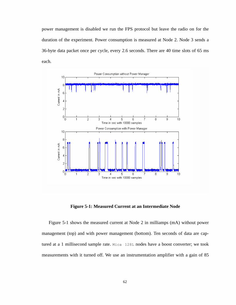
power management is disabled we run the FPS protocol but leave the radio on for the

duration of the experiment. Power consumption is measured at Node 2. Node 3 sends a

36-byte data packet once per cycle, every 2.6 seconds. There are 40 time slots of 65 ms

each.

Figure 5-1: Measured Current at an Intermediate Node

Figure 5-1 shows the measured current at Node 2 in milliamps (mA) without power

management (top) and with power management (bottom). Ten seconds of data are cap-

tured at a 1 millisecond sample rate. Mica 128L nodes have a boost converter; we took

measurements with it turned off. We use an instrumentation amplifier with a gain of 85

62

and measure voltage across a 1.1 Ohm resistor with an oscilloscope. Hence the current in

mA is:

Current [mA] = (voltage [V] / (85 * 1.1) ) * 1000

The average current measured is 8.144 mA with power management disabled; when

enabled it is 1.412 mA. A high-performance AA battery has a capacity of ~1800 mA-

hours. So, when power management is disabled the average battery life is 221.02 hours

(~9 days); when enabled it is 1274.79 hours (~53 days). Again, these figures are calcu-

lated for a mica mote with an RFM radio transmitting and forwarding data at a 2.6 second

sample rate.

While in its steady state, a node can be in 1 of 5 states in each time slot: Transmit (T),

Receive (R), Receive Pending (RP), Adaptive Advertisement (AA), or Idle (I). The Slack-

ers codebase uses Adaptive Advertisements (AA), described in Section 3.5.3, to synchro-

nize nodes, so we will not observe Communication Broadcast (CB) slot states. In the

steady state we will also not observe Transmit Pending (TP) slot states since no TxAdv

messages are being responded to.

By analyzing our session log we can determine the schedules of each node; as shown

in Table 5-1.

Table 5-1: Calculation of Duty Cycle from Observed Schedules

Node T R RP AA I Duty Cycle

1 3 2 2 1 32 20 %

2 2 1 2 1 34 15 %

3 1 0 0 0 39 2.5 %

63

For example, Node 1 has 3 T slots and 2 R slots. Now we can determine the expected

duty cycle for each node. Table 5-1 displays the count of slot states in the schedule of each

node. The duty cycle is the number of active slots per cycle divided by the total slots in a

cycle. For a cycle length of 40 time slots, the expected duty cycle for Node 2 is 15% (6/

40).

To determine the actual duty cycle measured at Node 2 over 10 seconds, we count the

number of samples in which Node 2 registers a current greater than 4 mA and divide this

by the total number of samples in the 10 second period:

1455 samples / 10000 samples = 14.55% duty cycle

This empirical calculation closely matches the theoretical 15%. Since the 10-second

window represents about 3.85 cycles and not an integral number, we expect some small

deviation from the theoretical results. As a comparison to the time-based duty cycle com-

putation, we can calculate the change in energy expenditure when the power management

protocol is enabled. We divide the average current measured with power management

enabled by that measured with power management disabled.

1.412 mA / 8.144 mA = .1734

If the sleeping current draw of the node were zero, we would expect this 17% value to

match the duty cycle. However, the microprocessor still draws current when the radio is

powered-down, so the ratio is slightly higher. We are uncertain why the peak current draw

64

using the power management protocol is below that of the disabled case, but were these

two values equal, the 17% calculated would rise another few percentage points.

5.2 Scheduled vs Unscheduled

In this section we present the results of two sets of experiments evaluating the effects of

network scheduling in multihop networks on contention, end-to-end fairness, and through-

put. We compare one set of experiments that uses scheduled communication, FPS, to a

second set that uses unscheduled communication, Naive store-and-forward. In the FPS

experiments, communication is scheduled, i.e., the send queue is managed by FPS. In the

Naive case, communication is unscheduled, i.e., the send queue policy is store-and-for-

ward — messages are put on the send queue upon arrival and immediately forwarded.

Otherwise, the code and all other parameters are the same for both sets of experiments,

and the radio is on the entire time.

We use two metrics in our evaluation: back off counts to measure the level of conten-

tion in the network (Section 5.2.1) and yield to measure end-to-end fairness and through-

put (Section 5.2.2).

Figure 5-2 shows 10 mica motes arranged in the 3-hop topology used in each experi-

ment. The arrows indicate transmit and receive pairs. The square represents one additional

mote connected to a PC, which serves as a base station. Two different configurations are

used. In the first configuration, motes are arranged as above in an 8' x 3'4" area. In the sec-

ond, the 10 motes are dispersed across five areas of a building, each mote between 9 and

22 feet apart. The two configurations of motes use the same topology, which is enforced in

software. One exception occurred due to hardware failure; in the Naive experiments mote

65

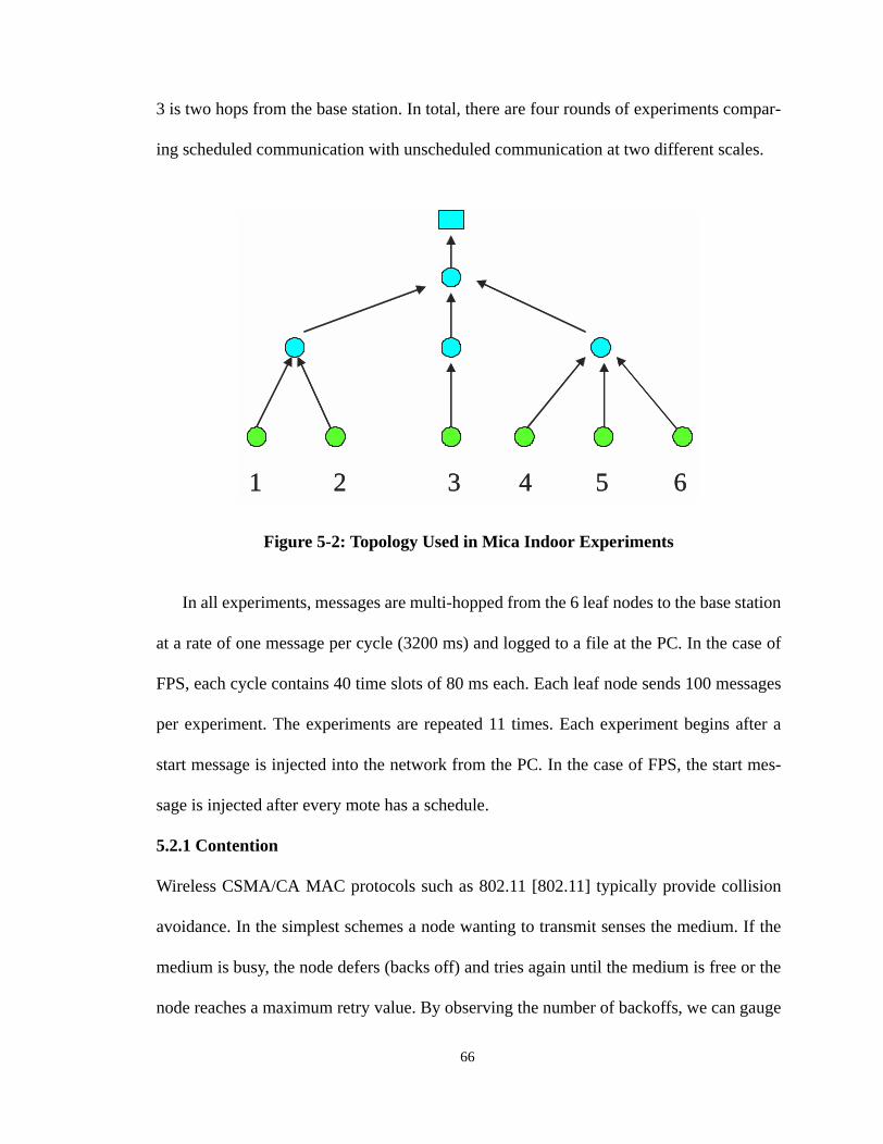
3 is two hops from the base station. In total, there are four rounds of experiments compar-

ing scheduled communication with unscheduled communication at two different scales.

Figure 5-2: Topology Used in Mica Indoor Experiments

In all experiments, messages are multi-hopped from the 6 leaf nodes to the base station

at a rate of one message per cycle (3200 ms) and logged to a file at the PC. In the case of

FPS, each cycle contains 40 time slots of 80 ms each. Each leaf node sends 100 messages

per experiment. The experiments are repeated 11 times. Each experiment begins after a

start message is injected into the network from the PC. In the case of FPS, the start mes-

sage is injected after every mote has a schedule.

5.2.1 Contention

Wireless CSMA/CA MAC protocols such as 802.11 [802.11] typically provide collision

avoidance. In the simplest schemes a node wanting to transmit senses the medium. If the

medium is busy, the node defers (backs off) and tries again until the medium is free or the

node reaches a maximum retry value. By observing the number of backoffs, we can gauge

1 2 3 4 5 61 2 3 4 5 6

66

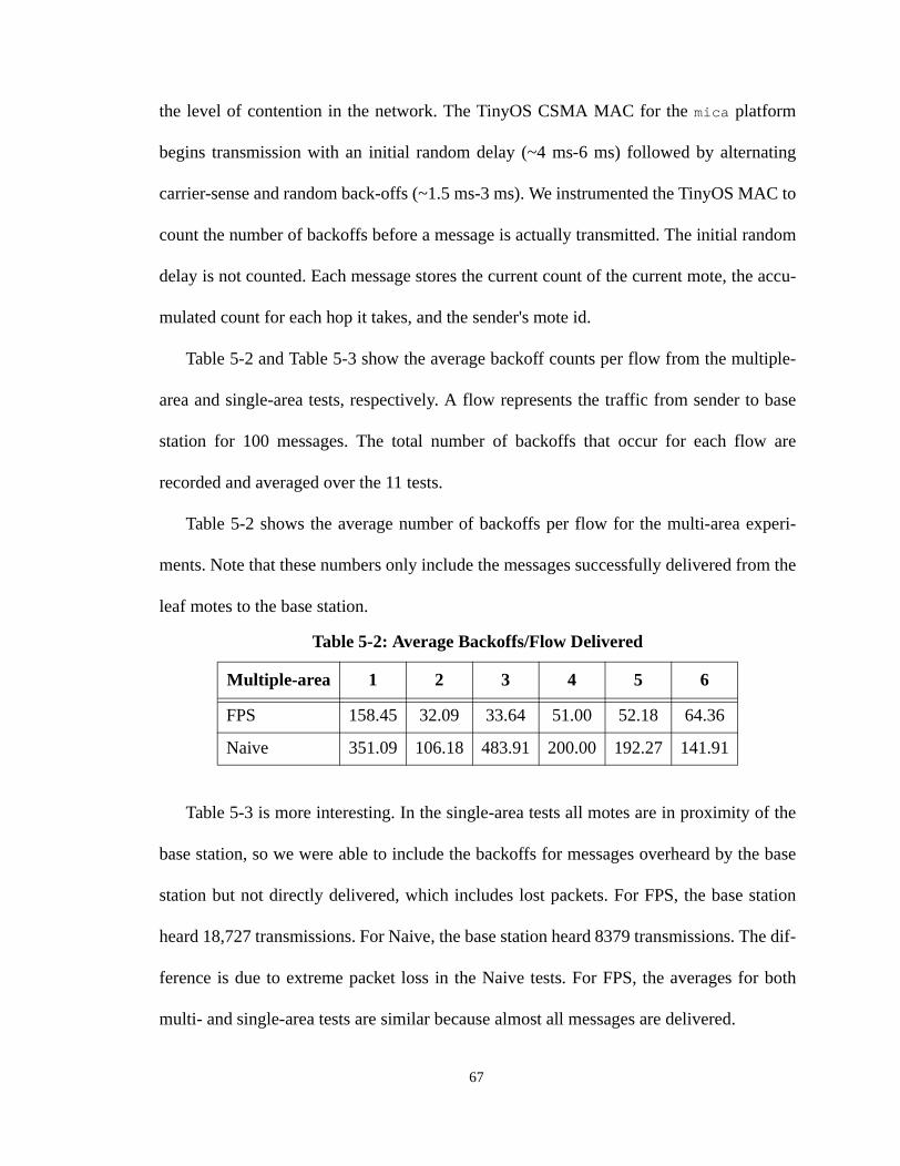
the level of contention in the network. The TinyOS CSMA MAC for the mica platform

begins transmission with an initial random delay (~4 ms-6 ms) followed by alternating

carrier-sense and random back-offs (~1.5 ms-3 ms). We instrumented the TinyOS MAC to

count the number of backoffs before a message is actually transmitted. The initial random

delay is not counted. Each message stores the current count of the current mote, the accu-

mulated count for each hop it takes, and the sender's mote id.

Table 5-2 and Table 5-3 show the average backoff counts per flow from the multiple-

area and single-area tests, respectively. A flow represents the traffic from sender to base

station for 100 messages. The total number of backoffs that occur for each flow are

recorded and averaged over the 11 tests.

Table 5-2 shows the average number of backoffs per flow for the multi-area experi-

ments. Note that these numbers only include the messages successfully delivered from the

leaf motes to the base station.

Table 5-3 is more interesting. In the single-area tests all motes are in proximity of the

base station, so we were able to include the backoffs for messages overheard by the base

station but not directly delivered, which includes lost packets. For FPS, the base station

heard 18,727 transmissions. For Naive, the base station heard 8379 transmissions. The dif-

ference is due to extreme packet loss in the Naive tests. For FPS, the averages for both

multi- and single-area tests are similar because almost all messages are delivered.

Table 5-2: Average Backoffs/Flow Delivered

Multiple-area 1 2 3 4 5 6

FPS 158.45 32.09 33.64 51.00 52.18 64.36

Naive 351.09 106.18 483.91 200.00 192.27 141.91

67

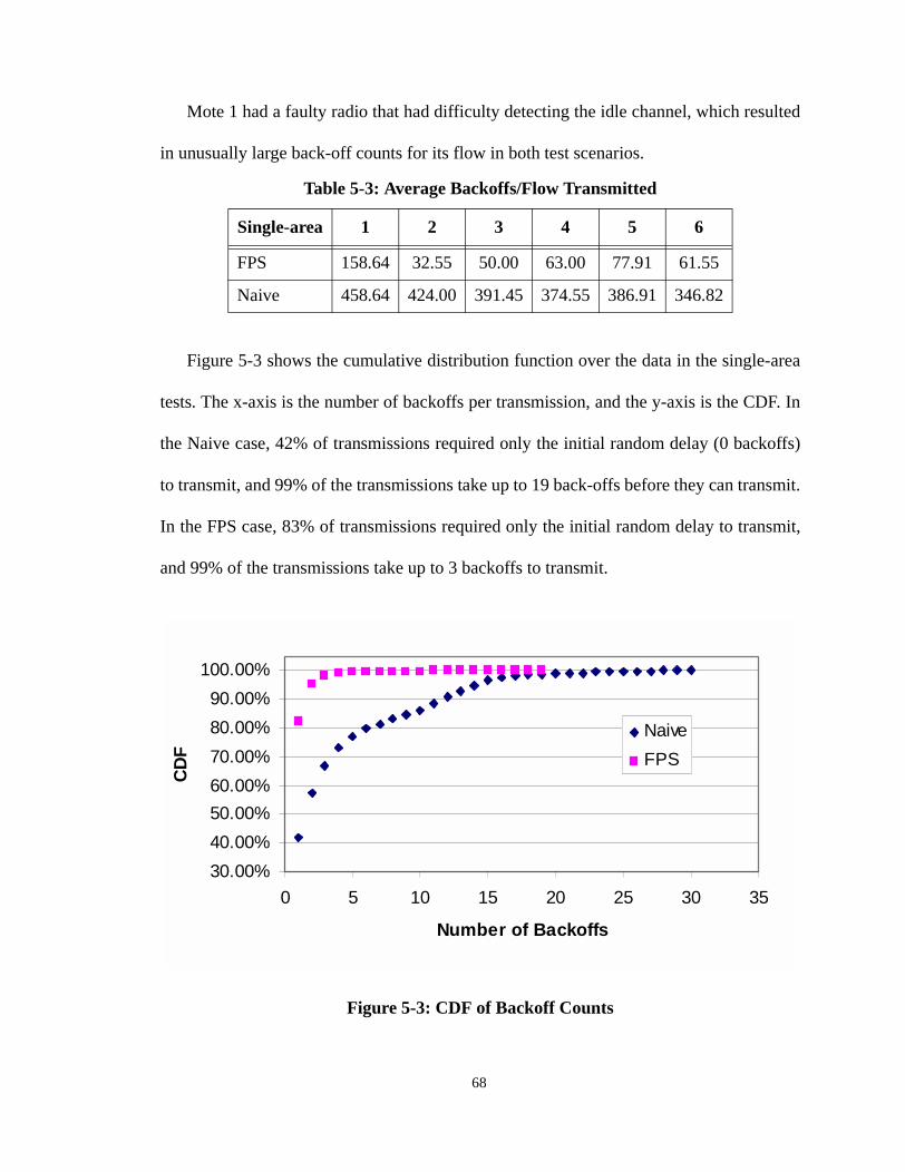
Mote 1 had a faulty radio that had difficulty detecting the idle channel, which resulted

in unusually large back-off counts for its flow in both test scenarios.

Figure 5-3 shows the cumulative distribution function over the data in the single-area

tests. The x-axis is the number of backoffs per transmission, and the y-axis is the CDF. In

the Naive case, 42% of transmissions required only the initial random delay (0 backoffs)

to transmit, and 99% of the transmissions take up to 19 back-offs before they can transmit.

In the FPS case, 83% of transmissions required only the initial random delay to transmit,

and 99% of the transmissions take up to 3 backoffs to transmit.

Figure 5-3: CDF of Backoff Counts

Table 5-3: Average Backoffs/Flow Transmitted

Single-area 1 2 3 4 5 6

FPS 158.64 32.55 50.00 63.00 77.91 61.55

Naive 458.64 424.00 391.45 374.55 386.91 346.82

30.00%

40.00%

50.00%

60.00%

70.00%

80.00%

90.00%

100.00%

0 5 10 15 20 25 30 35

Number of Backoffs

CD

F

Naive

FPS

68

We draw two conclusions from these results. First, communication scheduling reduces

contention in the network. It disperses transmission events such that they are not simulta-

neously contending for the medium. This is particularly important for multihop sensor net-

works in which traffic is often correlated. Second, FPS complements the underlying

CSMA MAC-layer, as shown by the fact at most 3 back-offs were required to transmit

99% of the time.

5.2.2 Fairness and Throughput

Wireless links are inherently lossy, and multihop wireless networks additionally suffer

from end-to-end packet loss. Yield, the number of packets received at the destination, is

often used to measure packet loss in multi-hop networks. Link-layer retransmission, adap-

tive rate control, and channel-switching are popular techniques for countering loss in wire-

less sensor networks. These methods operate at the link layer, and while effective, they

cannot detect or break end-to-end traffic correlations. A major source of contention is traf-

fic flows interfering with themselves and others. We use yield as a measure of both

throughput and end-to-end fairness among traffic flows. For all our experiments we use

the standard TinyOS CSMA MAC for the mica platform with no retransmission, rate con-

trol, or channel switching, so that we may observe the actual effect FPS has on end-to-end

fairness and throughput.

Figure 5-4 shows the percentage of messages received at the base station for FPS and

Naïve in the multi-area tests. The single-area tests are similar, and we do not show them

here. The x-axis is the sending mote id, and the y-axis is the percentage. Note that in the

Naïve tests, mote 3 is only two hops from the base station. This accounts for the higher

69

yield and illustrates the difference in packet loss between 3 and 2 hops. The overall

throughput is 96% for FPS versus only 25% for Naïve (despite its advantage on mote 3).

Figure 5-4: Fairness and Yield

When comparing flows for fairness, we do not include mote 3 for Naïve, since it only

included two hops. One measure of fairness is the standard deviation of the throughput

across the flows, which is +/- 1.13% for FPS and +/- 6.2% for Naïve. Thus, FPS has sig-

nificantly less variation as well as higher throughput. Second, we compute the ratio of the

max and min throughputs; if the approach is fair this ratio should be small. For FPS, the

0

10

20

30

40

50

60

70

80

90

100

FPS

Naive

1 2 3 4 5 6Motes

Cou

nt

0

10

20

30

40

50

60

70

80

90

100

FPS

Naive

1 2 3 4 5 6Motes

Cou

nt

70

ratio is only 1.03, versus about 2.5 for Naïve (Table 5-4). We conclude that communica-

tion scheduling does indeed increase throughput and end-to-end fairness.

* excludes mote 3 (see text)

Finally, note that although we did not use link-layer retransmission or parent-switch-

ing in these experiments, we still achieved excellent end-to-end throughput. These tech-

niques are largely complementary to FPS, and parent-switching (Section 4.4.1) has been

used with FPS successfully.

5.3 Duty Cycle and Latency

Traditionally there is a trade-off between duty cycle (periodic listen and sleep) and latency

(the time it takes to forward a message to the root). Any scheduling scheme will impose

larger per-hop latencies than those that store and immediately forward. If scheduling

occurs in units of one slot every cycle, and assuming messages are forwarded in FIFO

order, then it can take up to an entire cycle to forward a packet to the next hop. Thus, duty

cycle length is inversely proportional to cycle length. If cycles are very large, then this

may impose too much latency for some applications.

We use simulation to show the trade-off between worst case latency (one hop per

cycle) and duty cycle. Assume, for example, we have a 15-node binary tree (Figure 5-5) in

which each node generates a demand of one unit per node per cycle, yielding a total net-

Table 5-4: Throughput and Fairness

Approach Average STDDEV Max/Min

FPS 96.4 1.13 1.03

Naive 24.7 6.19* 2.48*

71

work traffic demand of 14 at the root. The traffic demand at each node is therefore the sum

of the demand of all its children plus one unit for itself.

Figure 5-5: 15-Node Binary Tree

The simulation calculates the overall network duty cycle and latency for sending mes-

sages 3-hops across the network from the leaves to the root for a given cycle length m, the

number of slots per cycle.

Figure 5-6: Duty Cycle vs Latency

0 500 1000 1500 2000 2500 30000

2

4

6

8

10

12

14

Latency [number of slot periods]

Ove

rall

duty

cyc

le o

f ne

twor

k [%

]

Duty cycle and latency in a 15-node test network

* m = 40

* m = 200

72

Figure 5-6 is a parametric graph with m as the parameter. The x-axis represents latency,

measured as the number of slots that occur from the time a message is sent from the leaf

nodes of the tree to the time it is received at the base station, as m increases from 30 to

1000 slots per cycle. In the simulation, one full cycle passes before forwarding a message

one level. This is the worst case scenario. For example, if m = 40 then X = 120

because there are 3 hops between leaf and root. The Y-axis represents the overall network

duty cycle, measured as the average amount of time the radio is on, as m increases from 30

to 1000 slots per cycle. For example, when m = 40, the duty cycle is approximately 9%,

and we expect to save approximately 91% of the original power in the network to satisfy a

demand of 14. When m = 200, the duty cycle is aproximately 2% and we expect to save

98% of the power. Lengthening the cycle time therefore the latency, but it saves more

power.

5.4 Optimized Latency Scheduling

In the simplest scheduling model of FPS, each flow reserves one slot per cycle for a given

child-parent link. This can lead to high latencies, as observed in Section 5.3, since a flow

makes only one hop of progress per cycle. We make two important optimizations to

reduce latency.

1. We order slots within a cycle so that the parent-grandparent slot occurs after

the child-parent slot. This allows multiple hops per cycle.

2. We allow fractional reservation of slots, which enable one transmission every

k cycles. This allows shorter cycle times without requiring more power,

since a fractional slot reservation requires k times less power. Thus we can

73

reduce latency by shortening the cycle time without increasing the required

power.

5.4.1 Reservation Window

FPS employs receiver inititated scheduling. The selection and assignment of reservation

slots is always made from the perspective of the receiving (route-through) node. We out-

line the steps to make a reservation below.

1. Parent selects an idle slot and advertises the slot.

2. Child hears the advertisement and sends a request for the slot.

3. Parent receives the request and sends an acknowledgement.

Here the parent node is the route-through node, closest to the base station. In Step 1,

FPS selects an idle slot at random from its entire cycle of slots. As a latency optimization,

we make a simple modification to the base protocol. Instead of selecting the slot from the

entire cycle, we select the slot from a subset called the reservation window.

Given a cycle length of size m, the reservation window is a sliding window whose size

is w where w <= m. The window begins w slots prior to the last transmit slot that the par-

ent node reserved with its parent (the grandparent). In this way, using only local informa-

tion, the slot being advertised to the child is always within w of the slot where it will be

forarded — putting an upper bound on the per hop latency of the network.

Other than w <= m, FPS does not restrict the value of w or whether it should be a

fixed global value or an adaptive local value. For example, FPS can easily be extended to

support some types of soft Quality of Service requirements by including the value of w in

protocol messages.

74

Figure 5-7: Reservation Window

Figure 5-7 shows a high-level view of 3 cycles of the schedule of a parent node that is

scheduling some route-through traffic. Here, the reservation window w = 4. In FPS,

since reservations are preallocated, the scheduling of transmit slots occurs before the

scheduling of receive slots as the algorithm seeks to keep a state of supply >=

demand. In Cycle 0, the last transmit slot was scheduled at slot 5, and since w = 4, the

next receive slot will be selected from between slots 1 and 4 in Cycle 1. Since the figure

depicts the parent node schedule, the reservation is marked R for receive in Cycle 2.

5.4.2 Fractional Flows

Fractional flows are not only a power optimization as discussed in Chapter 4, but also a

latency optimization. Instead of a node using one slot every cycle, a node may instead use

the slot once every k cycles, which allows for very infrequent slots without the need for

cycl

e0

1

2

0 1 2 3 4 5slot

Reservation Window

T

T

TR

cycl

e0

1

2

0 1 2 3 4 5slot

Reservation Window

T

T

TR

75

long cycles. An application designer can reduce latency by decreasing the cycle time,

since this will reduce delays in a multihop network. Without fractional flows, such a

decrease implies an increase in power as shown in Section 5.3, since a node is sending

more often. With fractional flows, the designer can change some nodes to fractional slots

to maintain a consistent power profile as cycle time decreases. Combined with reservation

windows, which coordinate the schedule, fractional flows allow fine-grain control over

the tradeoff between latency and power savings.

5.5 Partial Flows and Broadcast II

A Broadcast Channel is an instance of a partial flow (described in Section 3.4.2). In FPS,

upon joining the network, each node acquires at least one partial flow reservation that ter-

minates at its parent. This Comm channel is used by the node as a broadcast channel for

sending synchronization packets and advertisements. FPS protocol messages always

include the slot number of the Comm channel. In this way, child nodes know in which slot

to listen for broadcasts from their parent.

The Comm channel is also used for forwarding messages injected from the base sta-

tion. FPS maintains two forwarding queues. The SendQueue first is used for forwarding

packets toward the base station. The CmdQueue is used for forwarding commands away

from the base station. Forwarding queues are discussed further in Chapter 8.

When a node receives a command message it invokes the appropriate command han-

dler and places the message on the CmdQueue for forwarding. The Comm channel is

shared; both injected commands and synchronization packets use the same channel. The

76

convention is that commands to be forwarded are sent first, followed by the time sync

packet.

if current slot == Comm slotif command in command queue

broadcast command messageendif

broadcast sync packetendif

The GDI application in Chapter 6 uses the Comm channel for time sync packets and

injecting commands to start and stop the experiments. The TinyDB application in Chapter

7 uses the Comm channel for time sync packets and injecting TinyDB queries.

77

Chapter 6

Application: Great Duck

Island

In this section, we evaluate FPS on a real-world sensor network application, GDI

[Main02,Szew04], and show through laboratory experiments that FPS decreases conten-

tion, increases end-to-end fairness and throughput, and saves more power than the low-

power listening scheme currently used for this application.

6.1 Great Duck Island

GDI is a habitat monitoring application deployed on Great Duck Island, Maine. It is a

sense-to-gateway application that sends periodic readings to a remote base station, which

logs the data to an Internet-accessible database. The architecture is tiered, consisting of

two sensor patches, a transit network, and a remote base station. The transit network con-

sists of three gateways and connects the two sensor patches to the remote base station. The

78

two classes of mica2dot hardware are the burrow mote and the weather mote. The burrow

motes monitor the occupancy of birds in their underground burrows and the weather motes

monitor the climate above the ground surface. In this chapter, we will draw on information

about the weather motes provided by the study of the Great Duck Island deployment

[Szew04].

Of the two sensor patches, one is a singlehop network and the other is a multihop net-

work. The singlehop patch is deployed in an ellipse of length 57 meters and has 21

weather motes. Data is sampled and sent every 5 minutes. The multihop network is

deployed in a 221 x 71 meter area and has 36 weather motes. Data is sampled and sent

every 20 minutes.

In this chapter we compare the end-to-end packet reception, or yield, and power con-

sumption of GDI using FPS Twinkle1 with GDI using low-power listening [Hill02]

employed at Great Duck Island. We will also investigate the phenomena of overhearing in

the low-power listening case.

6.2 GDI with Low-Power Listening

The GDI application uses low-power listening to reduce radio power consumption. The

radio periodically samples the wireless channel for incoming packets. If there is nothing to

receive at a sample, the radio powers off, otherwise it wakes up from low-power listening

mode to receive the incoming packet. Messages include lengthy preambles, so they are at

least as long as the radio channel sampling interval. The advantages of low-power listen-

ing are that it reduces the cost of idle listening, integrates easily, and is complementary

1. Twinkle is the FPS codebase used with applications.

79

with other protocols. It is characterized, however, by a reliability-power tradeoff. Long

preambles mean long channel sampling intervals and more power is saved. However, as

the preambles get longer the end-to-end packet reception becomes poorer because in effect

it is congesting the network.

Density and multihop also impact power consumption. The GDI study [Szew04]

reports a much higher power consumption in the multihop patch than the single hop patch

which resulted in a shortened network lifetime — 63 of the 90 expected days — for the

multihop patch. Two causes are attributed. First, messages have a higher transmission and

reception cost due to their long preambles. Second, nodes wake up from low-power listen-

ing mode not only to receive their own packets, but anytime a packet is heard, regardless

of the destination. Overhearing is the main contributor to the higher power consumption in

the multihop patch. An independent TinyDB study [TASK05] confirms these findings as

well.

We also observe that although low-power listening reduces the cost of idle listening it

does not reduce the amount. Thus, at very low data-sampling intervals its advantage

declines because the radio must continue to turn on to check for incoming packets

although there are none to receive. For very low data rates, we will show that scheduling

such as FPS becomes more attractive because the radio (and potentially other subsystems)

can be deterministically powered down until they need to be used.

6.3 GDI with FPS

We implemented a version of GDI in TinyOS that uses FPS Twinkle for its radio power

management. This rather straightforward integration consisted of wiring the GDI applica-

80

tion component to the Twinkle component and disabling low-power listening. The

Vanderbilt TimeSync, SysTime, and SysAlarm [Maro04] components are used for time

synchronization and timers. At the time of this work, TimeSync only supported the use of

SysTime, which uses the CPU clock, so GDI was not able to power manage the CPU dur-

ing these experiments. In all data presented here we subtracted the draw of the CPU as if

we had used a low-power Timer implementation.

6.4 Experimental Setup

We conducted a total of 12 experiments on two versions of the GDI application. GDI-lpl

uses low-power listening and GDI-Twinkle uses FPS for radio power management. The

experiments were run on a 30-node in-lab multihop sensor network of mica2dot motes.

FPS supports data-gathering type applications like GDI in which the majority of traffic

is assumed to be low-rate, periodic, and traveling toward a base station. We ran a simple

routing tree algorithm provided by Twinkle based on grid locations to obtain a realistic

multihop tree topology and then used the same tree topology for the 12 experiments. Con-

sistent with the Great Duck Island deployment, no retransmissions are used in these exper-

iments.

In the experiments we varied the data sample rate: 30 seconds, 1 minute, 5 minute, and

20 minutes. For experiments with 30 second and 1 minute sample rates, 100 messages per

node were transmitted. For experiments with 5 minute and 20 minute sample rates, 48 and

12 messages were transmitted per node, respectively. In the GDI-lpl experiments we var-

ied the channel sampling interval: 485 ms and 100 ms. All experiments collected node id,

sequence number, routing tree parent, routing tree depth, node temperature, and node volt-

81

age. The GDI-Twinkle experiments also collected the number of children, number of

reserved slots, current transmission slot, current cycle, and number of radio-on slots per

sample period.

6.5 Measuring Current

During the experiments we measured the actual current at two nodes located in different

places of interest in the network. The inner node, is located one hop from the base station

and has a heavy amount of route-through traffic that is similar to its one-hop siblings. This

should give us an estimate of the maximum lifetime of the network. The leaf node is one

hop from the base station as well. As it does not route-through any traffic, we should be

able to see the effect of overhearing on power consumption at a node in a busy part of the

network.

At the lower sample rates, it is not feasible to take measurements over the entire sam-

ple period, so we designed our experiments so that we could take some measurements and

extrapolate others. For GDI-Twinkle, we define a cycle to be 30 seconds and schedule

using fractional flows (Section 5.4.2). Thus, a full sample period for the 30-second, 1-

minute, 5-minute, and 20-minute sample rates are 1, 2, 10, and 40 cycles respectively. For

taking the power measurement only, we schedule all traffic during one cycle of each sam-

ple period called the active cycle. The unscheduled cycles are called passive cycles. We

then measure the current at the two motes capturing data from both active and passive

cycles during the 1 minute sample rate experiment. Then we take a running windowed

average over a full 1-minute period, which gives us the power draw for both an active and

a passive cycle. Table 6-1 presents these direct power measurements.

82

Table 6-1: Power Measurement (mW)

For GDI-lpl we follow a similar method. We measure current at the two motes captur-

ing data from both active and passive periods during the 1-minute sample period experi-

ment. To represent an active period, we take a running average over the full 1-minute

period. This also captures all the overhearing that occurs at the mote during a full period of

any given sample rate. To represent a passive period, we took the longest chain of data

from the measurements in which only idle channel sampling occurred. From this informa-

tion we calculate the power consumption for the 5-minute and 20-minute sample rate

experiments. The 30-second sample rate was measured separately (not calculated) and is

shown in Figure 6-1.

6.6 Evaluation

In this section we discuss the results of the data from all 12 experiments and we compare

with actual GDI deployment data.

6.6.1 Power Comparison with Low-Power Listening

Given the direct power measurements from Table 6-1, we can calculate the power con-

sumption for the 5-minute and 20-minute sample rate experiments. For example, for Twin-

PowerManagement

Period(Sec)

Inner(mW)

Leaf(mW)

Twinkle active 30 2.18 0.69

Twinkle passive 30 0.33 0.33

Lpl-485 active 60 16.5 16.0

Lpl-485 passive 60 0.99 0.99

Lpl-100 active 60 8.20 7.60

Lpl-100 passive 60 3.90 3.90

83

kle we read off the following: an active cycle at the inner mote consumes 2.18 mW and a

passive cycle consumes 0.33 mW. Given these numbers, for a 20-minute sampling rate we

expect 1 active cycle and 39 passive cycles, for a weighted average of 0.38 mW. For the

leaf mote, an active cycle consumes 0.69 mW and a passive cycle consumes 0.33 mW,

giving a weighted average of 0.34 mW.

We compute the GDI-lpl power consumption for the 5-minute and 20-minute experi-

ments similarly. For example, for GDI-lpl at a 20-minute sample rate we assume that for

one minute the application consumes the energy of the active period and for the remaining

19 minutes the application consumes the energy of the passive period. Using the values

from Table 6-1, the inner mote during the 20-minute sample rate Lpl-100 experiment

would consume an average of 4.12 mW ((8.2+19*3.9)/20 = 4.12mW).

Figure 6-1 through Figure 6-4 show all four sample periods: the 30-second and 1-

minute rates are measured, and the 5-minute and 20-minute periods are calculated as

described above. For FPS Twinkle, the inner node consistently has a greater draw than the

leaf node. In contrast for LPL, the inner and leaf nodes consistently have almost the same

draw. This indicates that FPS's main power draw depends on the routed traffic, and in

most cases LPL's main power draw depends on the overheard traffic. However, from

Table 6-1 we see that the passive power draw for LPL-100 is 3.9 mW, which forms an

asymptote as the sample period increases. Overall, as the sample rate decreases and the

preambles shorten, overhearing plays a lesser role and the frequency of channel sampling

plays a bigger role.

84

Figure 6-1: 30 Second Sample Period

Figure 6-2: 1 Minute Sample Period

0

5

10

15

20

25

30

Inner Leaf

Po

wer

(m

W)

TwinkleLpl-485Lpl-100"Pulse"

0

5

10

15

20

Inner Leaf

Po

wer

(m

W)

85

Figure 6-3: 5 Minute Sample Period

Figure 6-4: 20 Minute Sample Period

0

2

4

6

8

10

Inner Leaf

Po

wer

(m

W)

TwinkleLpl-485Lpl-100Pulse

0

1

2

3

4

5

6

Inner Leaf

Po

wer

(m

W)

86

In addition, at the higher sample rates, LPL-485 has a higher power consumption than

LPL-100, but at the lower sample rates the opposite is true. This reveals a relationship

within LPL in which the cost of transmitting increases with longer preambles, the cost of

channel sampling decreases with longer sampling intervals.

Finally, we added a newer variation of LPL to the power figures above, called Pulse.

Pulse was developed as part of BMAC [Pola04], and it optimizes the power consumption

of LPL by listening for energy in the channel rather than a decoded preamble. This

reduces the cost of listening substantially. We can compute the active and passive esti-

mates for Pulse given our power traces and Table 2 from the BMAC paper, which provides

the raw listening cost. Although Pulse does perform better than LPL, it is still has 2x to 5x

higher power consumption than FPS.

Across the board, FPS has better power consumption than LPL, with improvements

that range from 2x (over Pulse for low rates) to 10x (in cases where the listening interval is

poorly chosen).

6.6.2 Yield and Fairness

Table 6-2 shows the average yield for all 12 experiments as well as the ratio of the best

and worst throughputs (Max/Min). This ratio indicates fairness: lower ratios are more fair.

At 30 seconds, the LPL-485 network is saturated due to the long preambles, which

accounts for its low yield. Overall, both FPS and LPL-100 are significantly better than

LPL-485. FPS shows better fairness than LPL-100, and, other than the 30 second sample

rate, FPS has higher yield than LPL-100.

87

Table 6-2: Yield and Fairness Comparison

6.6.3 Comparison with GDI Deployment

A comparison to the data provided by the GDI study [Szew04], shows that the results

in the laboratory and field are remarkably similar. The Great Duck Island deployment used

a low-power listening channel sampling interval of 485 ms, a data sample period of 20

minutes in the multihop patch, and a sample period of 5 minutes in the singlehop patch.

Table 6-3 presents results taken from the GDI field study, labeled GDI-485, and

includes data from four of our in-lab experiments, labeled LPL-485 and Twinkle. For each

row, we report the sample period, average yield, inner and leaf power consumption, and

the number of nodes in the experiment. For GDI-485, the yield figure represents the aver-

age yield from the first day of deployment.

PowerScheme

SamplePeriod

YieldMax/Min

Twinkle 0.5 0.80 2.11

Twinkle 1 0.90 1.74

Twinkle 5 0.84 1.92

Twinkle 20 0.83 2.4

Lpl-485 0.5 0.40 15.6

Lpl-485 1 0.68 94.0

Lpl-485 5 0.72 11.8

Lpl-485 20 0.69 12.0

Lpl-100 0.5 0.85 3.45

Lpl-100 1 0.83 2.23

Lpl-100 5 0.78 2.76

Lpl-100 20 0.77 4.00

88

Table 6-3: Lab and Deployment Comparison

A close comparison can be drawn between LPL-485 and GDI-485 at the 20 minute

sample rate. LPL-485 has a power draw of ~1.76 mW while GDI-485 has a power draw of

1.6 mW. The GDI-485 figure is expected to be lower for two reasons. In the laboratory, the

two measured nodes are from the busier section of the testbed, and the testbed has a con-

stant load rather than a decreasing one. In the GDI deployment, some multihop motes died

and stopped sourcing traffic, which is why we report yield only from the first day of

deployment.

The yield data is extremely similar as well. All yields for LPL-485 and GDI-485 are

~70%. The only large difference between the two data sets is the power consumption at

the 5-minute sample period. This is easily explained; at the 5-minute sample period, GDI-

485 is singlehop while LPL-485 is multihop, and the LPL-485 measurements include a

large amount of overhearing. Given the closeness of LPL-485 and GDI-485, the FPS

Twinkle numbers are a good estimate of how FPS would have performed. In particular,

FPS consumes at least 4X less power and provides about 14% better yield.

Power Mgnt

SamplePeriod

Yield Inner(mW)

Leaf(mW)

#

GDI-485(single)

5 0.70 n/a 0.71 21

GDI-485(multi)

20 0.70 1.60 n/a 36

Lpl-485 5 0.72 4.09 3.99 30

Lpl-485 20 0.69 1.77 1.74 30

Twinkle 5 0.84 0.52 0.36 30

Twinkle 20 0.83 0.38 0.34 30

89

Chapter 7

Application: TinyDB

In this chapter, we evaluate FPS on a real-world sensor network application, TinyDB

[TinyDB02,TASK05], and show that FPS decreases power consumption by 4.3X over

TinyDB’s application-level duty cycling approach. TinyDB is a good candidate applica-

tion for FPS because its most basic requirements are precisely the features that FPS does

well:

1. Power management

2. Robust end-to-end packet reception

3. Multiple queries

4. Query dissemination

5. Time synchronization.

The most pressing problems facing TinyDB (or TASK) today are the dual issues of

power consumption and packet loss that are still unacceptably high for many deployments

[TASK05]. This is primarily due to the tradeoff between power consumption and end-to-

end packet reception inherent in the application level “duty cycling” TinyDB uses. All

90

duty cycling schemes have this problem in multihop networks because these protocols aim

to synchronize the network to transmit all packets at the same or near same time. FPS

solves the reliability-power tradeoff by scheduling traffic randomly while power schedul-

ing, as shown in Chapter Chapter 5.

In addition, duty cycling constrains the use of multiple queries, which is a significant

feature in TinyDB. The duty cycle parameter is fixed and set at compile time, so additional

queries cannot be added. Because FPS is adaptive, it can support multiple queries.

FPS also supports query dissemination and time synchronization, both very imporant

features for TinyDB. Not only is it necessary to inject queries, but injecting commands is

also important for network management. Time synchronization is essential for sensor

reading correlation. Moreover, all requirements listed are accomplished by FPS in the

presence of power management.

7.1 TinyDB

TinyDB is a distributed query processor for TinyOS motes. TinyDB consists of a declara-

tive SQL-like query language, a virtual database table, and a Java API for issuing queries

and collecting results.

Conceptually the entire network is viewed as a single table called sensors in which

the attributes are inputs of the motes (e.g., temperature, light). Queries are issued against

the sensors table via the Java API and disseminated throughout the network. The SQL lan-

guage is extended to include an “EPOCH DURATION” clause that specifies the sample

rate. A typical query looks like this:

91

SELECT nodeid, temperatureFROM sensorsEPOCH DURATION 3 min

TinyDB allows up to two concurrent queries: one for sensor readings and one for net-

work monitoring. In theory, TinyDB can support multiple concurrently running queries,

but, the current strategy for duty cycling and synchronization of sensor data readings has

had implications for what is actually feasible. To FPS, queries in general are viewed as

increases or decreases in demand. The notion of why a change in demand occurs (e.g.,

whether it is one or more queries) is transparent to FPS. This makes TinyDB an ideal tar-

get application for FPS.

In this chapter we compare the power savings of TinyDB using FPS versus TinyDB

using application level “duty cycling” — the power management scheme currently used in

TinyDB. We estimate the power savings of the two approaches using the TinyDB Red-

wood deployment of 35 motes, conducted October 2003 in the Berkeley Botanical Garden

[BotGar04], for our topology and traffic models.

7.2 Estimating Power Consumption

As it is not feasable to directly measure the power consumption of 35 motes, we use the

following three-part methodology:

1. Estimate the amount of time the radio is on and off for each scheme. Our

metric for this will be radio on time per hour, measured in seconds.

2. For FPS, we validate this estimate in Section 7.6 by looking in detail at one

of the motes. The radio on time for duty cycling is easy to estimate.

92

3. We use actual measured current from mica and mica2 motes to estimate

power consumption for radio on/off times. (In the GDI application,Chapter 6,

we measured the current directly during the experiment.)

This combination provides a reasonably accurate overall view of power consumption,

which although not perfect is certainly very accurate relative to the 5X advantage in power

shown by FPS.

7.3 The Redwood Deployment

The Redwood deployment has 35 mica2dot motes dispersed across two trees reporting to

one base station in the Berkeley Botanical Gardens. Each tree has 3 tiers of 5 nodes each

and 2 nodes placed at each crest. One tree has 1 additional node at a bottom branch. Every

2.5 minutes each mote transmits its query results, which are multi-hopped and logged at

the base station.

The routing scheme uses LEPSM link estimation to parent switch, so the topology

changes over time. By examining the records in the redwood database, we derived the

actual topology information. From this a general topology depicted in Figure 7-1 was con-

structed that reflects the network’s state the majority of the time.

Figure 7-1: Sub-tree Redwood Deployment

0

1 2

3

00

11 22

33

93

Out of 35 nodes, generally 2/3 of the nodes are one hop and 1/3 of the nodes are two

hops from the base station at any given time. We start by computing the radio on time per

hour for the case with no power management:

60 sec/min * 60 min/hour = 3600 sec/hour

No power management = 3600 sec/hourNo power management = 3600 sec/hourNo power management = 3600 sec/hourNo power management = 3600 sec/hour

This number is the average amount of time each radio is on per hour for the whole

deployment. We next estimate this metric for duty cycling followed by an estimate for

FPS.

7.4 TinyDB with Duty Cycling

In TinyDB duty cycling, the default power management scheme, all nodes wake up at the

same time for a fixed waking period every EPOCH. During the waking period nodes

exchange messages and take sensor readings. Outside the waking period the processor,

radio, and sensors are powered down. Estimating the radio-on time is thus straightfor-

ward: all 35 nodes wake up at the same time every 2.5 minutes for 4 seconds and exchange

messages. The sample rate is thus 24 samples per hour. Each node is on for 96 sec/hour.

24 samples/hour * 4 sec/sample = 96 sec/hour

Duty Cycling = 96 sec/hourDuty Cycling = 96 sec/hourDuty Cycling = 96 sec/hourDuty Cycling = 96 sec/hour

As expected, this approach is subject to very high packet losses due to the contention

produced by exchanging packets at nearly the same time.

A recent TinyDB empirical study [TASK05] shows high losses, between 43% and

50%, and high variance using duty cycling. Although we did not test it explicitly, there is

94

no reason to expect the yield for FPS (or low-power listening) would deviate from the

80% shown in the previous chapter.

7.5 TinyDB with FPS

Topology, time-slot duration, advertising frequency, and sample rates are factors in esti-

mating the radio-on time for FPS. We will use the same topology as above for estimating

the radio-on time of the 35 nodes. The duration of a time slot is 128 ms, and the sample

rate is again once every 2.5 minutes.

Time-slot duration, number of slots per cycle, and advertising frequency are parame-

ters in FPS. The time-slot duration is dependent on the MAC and PHY layer characteris-

tics, but must be at least the time required to send two TinyDB messages. For this

example, the time slot duration is 128 ms and there are 1172 slots per cycle, which is

roughly 2.5 minutes. The advertising frequency is once per cycle.

Figure 7-2: Topology with Demand for Estimates

0

2

3

1

Comm

Traffic

0

2

3

1

0

2

3

1

Comm

Traffic

Comm

Traffic

95

Figure 7-2 depicts the subtree with its demand derived from the redwood database.

The lines in the graph are Transmit (T)-Receive (R) pairs representing FPS bandwidth res-

ervations between nodes. Solid lines represent the demand required in terms of one time

slot per cycle to forward traffic to the base station. The dashed lines represent a partial

flow, the Comm channel, used for TinyDB queries and network protocol messages. Each

end-point, except Node 0, is counted as one 128 ms time slot when the radio is on every

cycle. Node 3 has 2 T slots, Node 2 has 3 T slots and 2 R slots, and Node 1 has 2 T slots

for a total of 9 (T,R) time slots. Node 0 is the base station and has no cost. The additional

overhead per node for Adaptive Advertisments (AA) once per cycle is 3 time slots per

cycle: one T and two Rs.

For the three nodes the cost is 2.3 seconds for each cycle:

9 (T,R) + 3 (A)*(3 nodes)= 18 (T,R,A) * 128ms= 2.3 sec/cycle per 3 nodes= 0.767 sec/cycle (per node)

At 24 samples per hour, on average, each node is on 18.4 sec/hour:

24 samples/hour * 0.767 sec/cycle= 18.4 sec/hour

FPS = 18.4 sec/hourFPS = 18.4 sec/hourFPS = 18.4 sec/hourFPS = 18.4 sec/hour

This is a savings of 5.2X compared with the duty cycle approach and 196X compared

with no power management. In addition, the radio-on time is actually overestimated.

Transmit slots do not leave the radio on for the whole slot since they can stop once their

message is sent; this is shown in detail in the next section.

96

7.6 FPS Validation

We implemented a prototype of TinyDB that uses FPS Twinkle for radio power manage-

ment. To validate our prototype, we ran the following experiment on three mica2dot

motes and one mica2 mote as base station arranged in a topology shown in Figure 7-2. We

monitored intermediate Node 2 while it forwarded packets and sent advertisements once

per cycle. There are 64 slots of 128 ms each per cycle. We instrumented TinyDB-FPS to

record the time of each call to turn the radio on and radio off, the beginning time of each

time slot, and the state of each slot. From the TinyDB Java tool we issue the query:

SELECT nodeidFROM sensorsEPOCH DURATION 8192 ms

The intermediate mote is connected to an Ethernet device, and the debug records are

logged over the network to a file on the PC. The regular query results are multi-hopped to

the base station and displayed by the Java tool.

In this experiment, we expect to have 1 advertisement, 2 receive slots, 3 transmit slots,

2 receive pending slots, and 56 idle slots per 64-slot cycle. We validated both the use of

slots and the radio on/off times. The results are shown in Table 7-1 and Figure 7-3 below.

Note that the radio off time is higher than the percentage of idle slots because Transmit

slots turn the radio off early — as soon as their messages have been sent.

Table 7-1: Predicted vs. Measured Idle Time

Metric Slots Idle %

Predicted Idle Slots 56/64 89.1

Measured Idle Slots 56/64 89.1

Measured Radio Off Time — 91

97

Figure 7-3: Slot State and Radio State

Figure 7-3 shows a subsection of the validation experiment. The bottom graph shows

the measured FPS state versus time and the slot number; this section shows the active por-

tion of a cycle (slots not shown are idle). The top graph shows actual radio on/off times

(milliseconds). Note that the radio is always off for Idle slots and that for Transmit slots

the on time is just long enough to transmit the queued messages.

In this experiment, the time slot duration is 128 ms, there are 64 slots per cycle, and

the advertising frequency is once per cycle. This cut shows two advertising slots, which is

fine given that they are actually in two different cycles.

This experiment validates our methodology and shows that the power estimate for FPS

in the previous section is actually conservative (since we count all of the Transmit slot

time).

0

1

29 30 31 32 33 34 35 36 37 38 39 40 41 42 43 44 45 46 47 48 49 50 51 52 53 54 55 56 57 58 59 60 61 62 63 0 1 2 3 4 5 6 7 8 9

Slot Number

Sta

te

Advert

Receive

Transmit

Idle

0

1

143000 144000 145000 146000 147000 148000 T im e (m il l ise co n d s)O

n/O

ff

98

7.7 Power Savings

Finally, given the validated radio on times, we can estimate the power savings. First,

however we need to know the current draw for a mote depending on whether or not the

radio is on, and/or the CPU is on.

We obtained the results shown in Table 7-2 via an oscilloscope tracing the motes dur-

ing experiments with mica and mica2 motes. The mica uses an RFM radio and mica2 uses

a Chipcon radio. (The Chipcon radio power varies from 7.4 to 15.8 mA depending on

transmit power, plus 7.8 mA for the mica2 CPU for a total of 15.2 to 23.6 mA. We use

20mA as an overall estimate.) Given these current draws, we estimate power consumption

as:

Power (mAh) = (Radio-on time)*(On draw) + (Radio-Off time)*(Off draw)

Table 7-2: Power Consumption of Motes (mA)

Mote Asleep CPU CPU+Radio

Mica 0.01 0.4 8.0

Mica2 0.03 3.9 20

Table 7-3: Radio-on Times (seconds per hour)

Scheme Radio On Time Ratio

None 3600 196

Duty Cycling 96 5.2

Twinkle 18.4 1

99

Using this equation and the radio-on times summarized in Table 7-3, we estimate the

power consumption in Figure 7-4 and Figure 7-5. In all cases, both Duty Cycling and FPS

perform substantially better (lower power) than no power management, so we focus on the

difference between FPS and Duty Cycling.

Figure 7-4: Mica Estimates (mA-seconds)

Figure 7-4 and Figure 7-5 show the estimated power savings for two families of motes,

mica and mica2 respectively, with the CPU on or asleep when the radio is off. Each verti-

cal axis has a different scale, and in all cases the “no power savings” column goes off the

top (with the value shown). Light gray is the radio-off power consumed (per hour), while

dark gray is the radio-on power.

An important issue in estimating the power savings is whether or not the CPU is asleep

when the radio is off. Neither system needs the CPU per se during idle times, but some

100

sensors may require CPU power. Thus, we expect for both mica and mica2 that the “CPU

asleep” numbers are more realistic, and we will quote these in our overall conclusions.

However, we include the “CPU on” case for completeness.

Figure 7-5: Mica2 Estimate (mA-seconds)

Note that even for cases in which the CPU is needed for sensor sampling, the “CPU

asleep” graph is more accurate, since the CPU would be asleep most of the time. For the

“CPU on” case, FPS outperforms Duty Cycling by 37% on the mica and 8% on the mica2,

which has a higher CPU current draw. Compared to no power management, the advantage

for FPS is 18X and 5X, respectively.

For the more realistic “CPU asleep” case, i.e., the CPU is asleep during Idle slots, FPS

outperforms Duty Cycling by 4.4X on the mica and 4.3X on the mica2. Note that this is

consistent with the 5.2X reduction in radio on time (Section 7.5). Compared to no power

management, the advantage for FPS is 160X and 150X on the mica and mica2, respec-

101

tively. To summarize, for the TinyDB application with the Redwood study workload, FPS

has a power savings of about 4.3X over Duty Cycling and 150X over no power manage-

ment.

102

Chapter 8

Advanced Techniques

Good buffer management combined with queuing is vital for managing route-thru traffic

and scheduling. FPS explicitly manages the forwarding queues and provides a facility for

global buffer management. We believe these elements are essential not only for FPS, but

for emerging research in power-aware multihop routing, congestion control, and general

scheduling for sensor networks. In addition, we present a good random number generator

implemented for TinyOS.

8.1 Forwarding Queues

FPS maintains two forwarding queues: one for forwarding messages toward the base sta-

tion, the SendQueue, and one for forwarding messages away from the base station or

broadcasting, the CmdQueue. The architecture is such that policy is separated from mech-

anism. This not only allows the FPS power scheduler to set the forwarding policy, but also

allows other policies to be interchanged and investigated. Currently two policies are avail-

able: store-and-foward and FPS.

103

Figure 8-1 depicts the architecture at the network layer. Messages arrive at the router

component and are put on one of the forwarding queues. If the the message is a broadcast

or command, it is placed on the CmdQueue; otherwise, it is placed on the SendQueue with

the forwarding address selected by the route selector component.

Figure 8-1: Separating Policy from Mechanism

When a T or CB slot arrives in the local power schedule, the power scheduler compo-

nent signals the SendQueue or CmdQueue, respectively. All messages in the CmdQueue

use the broadcast address.

The striped arrows in the figure indicate the power scheduler sets the policy for the

forwarding queues and route selector. This is a fundamental difference between our archi-

tecture and existing approaches. Clearly, since FPS schedules radio on and off times the

forwarding queues must be managed. For the same reason the route selector cannot choose

or change parents without collaboration from FPS. In addition, FPS load balances as we

described in Section 3.5.1.

router

power schedulerroute selector

CmdQueue

SendQueue

forwarding queues

PolicyPolicy

MechanismMechanismNetwork Layer

router

power schedulerroute selector

CmdQueue

SendQueue

forwarding queues

CmdQueue

SendQueue

forwarding queues

PolicyPolicy

MechanismMechanismNetwork Layer

104

8.2 Global Buffer Management

The Buffer Manager is used by the network, application, and power scheduling compo-

nents. It consists of a global buffer cache partitioned into multiple “free lists” and a set of

queues. Each element (or buffer) of a free list or queue is a TinyOS message of type

TOS_Msg. The size of each free list and queue is set at compile time. Thus all message

buffers are preallocated at compile time and managed by the Buffer Manager at runtime.

Figure 8-2 shows the relationship between free lists and queues. The buffers of each

free list are reserved for their respective components. The SendQueue is shared by the

application and network components, the CmdQueue is used by the network component,

and the ProcessQueue is used by the power scheduling component. Queues are used in

two ways: as forwarding queues as described in Section 8.1 and as dispatchers, the Pro-

cessQueue for example, as described in Section 8.2.4. Once a buffer from a queue has

been consumed, the Buffer Manager returns it to the appropriate free list.

Figure 8-2: Global Buffer Manager

Global Buffer CacheApplication Network FPS

SendQueue CmdQueue ProcessQueue

Free Lists

Queues

completions

Global Buffer CacheApplication Network FPS

SendQueue CmdQueue ProcessQueue

Free Lists

Queues

completions

105

Free lists serve two functions: buffer allocation and buffer swapping. In Figure 8-2 a

solid straight arrow indicates buffer allocation and a dashed double arrow indicates buffer

swapping.

8.2.1 Application Bufffer Allocation

The Buffer Manager provides an interface, AllocSend, that allows the application to send

TinyOS messages without managing buffers. The allocation and freeing of buffers is han-

dled by the Buffer Manager and is transparent to the application layer.

Figure 8-3: Application Buffer Allocation

Figure 8-3 illustrates the use of buffer allocation. The application calls Alloc-

Send.allocBuffer() to get a free message buffer and then calls AllocSend.send() when it is

ready to send a message. The message is placed on the SendQueue for scheduling by FPS.

After the message is sent, the used buffer is returned to the application free list.

8.2.2 Network Buffer Swapping

The Buffer Manager offers useful functionality for buffer swapping between the TinyOS

network and messaging layers. When a network component receives a message, a specific

handler is invoked with the message buffer passed as an argument. The messaging layer

expects a message buffer to return quickly so it can be used for the next incoming mes-

SendQueueFree List

completion

application

allocSendQueueFree List

completion

application

alloc

106

sage. The current message buffer will not be available until the next T (or CB) time slot,

so a buffer is returned from the network free list and the current buffer is placed on one of

the forwarding queues.

Figure 8-4: Network Buffer Swapping

Figure 8-4 illustrates the use of network buffer swapping. If the incoming message is a

TinyOS command, type SimpleCmdMsg, it is placed on the CmdQueue, otherwise it is

placed on the SendQueue. After the message is sent, the used buffer is returned to the net-

work free list.

8.2.3 Determining Free Lists

As discussed previously, both application and network components use the same Send-

Queue to route messages toward the base station, however they use their own free lists in

two different ways. The application component uses its free list for buffer allocation and

the network component uses its free list for buffer swapping.

Each free list provides a method, List.member(), that takes a buffer pointer as an argu-

ment. When called, it determines whether the buffer belongs to this free list. After a mes-

sage has been sent, the Buffer Manager calls List.member() on the application free list. If

Forwarding Queues

Free List

networkmessaging

completion

swap

Forwarding Queues

Free List

networkmessaging

completion

swap

107

the buffer is a member of this list it is returned there, otherwise it is returned to the net-

work free list.

8.2.4 Message Processing

The FPS power scheduling component uses the Buffer Manager for buffer swapping and

protocol message processing. This allows FPS to easily handle the receipt of multiple pro-

tocol messages.

Figure 8-5: Process Message Queue

Figure 8-5 illustrates how the power scheduler uses its free list and ProcessQueue.

When the power scheduler component receives a protocol message, it swaps buffers with

the messaging layer, puts the incoming message on the ProcessQueue, and posts a TinyOS

task. A task is a TinyOS function whose execution is deferred. When the TinyOS task

runs, it dequeues the message from the ProcessQueue, does some work, and finally returns

the used message buffer to the FPS free list. The task that is posted corresponds to the type

of message received. For exampe, if RxReq is received and accepted, a task is posted to

execute TxConf.

Free List

power schedulermessaging

swap

taskProcessQueue

completion

Free List

power schedulermessaging

swap

tasktaskProcessQueue

completion

108

8.3 Pseudo-random Number Generation

In FPS the selection of reservation slots is random; good schedules depend on a good ran-

dom number generator. We coded a fast implementation of the Park-Miller Minimal Stan-

dard Generator [Park88] for pseudo-random numbers offered by Carta [Car90].

The implementation uses a 32 bit multiplicative linear congruential generator,

S' = (A x S) mod (231 - 1)

where S is the seed, S’ is the previous seed, and multiplier A = 16807.

The form of this algorithm is called Lehmer’s Algorithm. Park explains Lehmer’s

algorithm will yield a good minimal standard if:

1. the algorithm parameters (modulus and multiplier) are chosen properly

2. the software implementation is correct.

The prime modulus 231 - 1 is a standard among specialists because it allows for fast

implementation using 32-bit arithmetic. The multiplier 16807 is a good choice because it

will yield a full period generating function; one that does not repeat during the period. The

selection of multiplier is an ongoing area of research and A = 16807 is just one of more

than 534 million full period multipliers.

Park describes a test for a correct implementation of the minimal standard. We suc-

cessfully implemented and tested this algorithm with the above parameters using the fast

32-bit arithmetic outlined by Carta.

109

Chapter 9

Future Work

In this chapter we visit open issues and propose new areas of investigation that we hope to

and others will pursue in the future.

9.1 Power-aware Multihop Routing

Currently, there is no power-aware mulithop routing implementation in TinyOS. We

developed our own mulithop component based on simple grid routing for use in our test-

beds. To integrate with FPS, multihop routing components must be power-aware. We have

identified three requirements for this:

1. Separate queuing policy from mechanism

2. Buffer management

3. Parent selection interface in route selector module.

As discussed in Section 8.1 the main difference between our architecture and existing

approaches is the separation of queuing policy and mechanism of the forwarding queues.

110

We will refer to the new power-aware multihop routing architecture as lib/SchedRoute for

scheduled routing.

Figure 9-1: Power-aware Multihop Routing

Figure 9-1 shows the existing multihop routing design using lib/Route as an example

and the new design using lib/SchedRoute. First, SchedulePolicyC provides the policy for

the forwarding queues. In its simplest form it uses store-and-forward. For power schedul-

ing, it uses FPS. Second, QueuedASend (queued alloc send) provides buffer management

and manages multiple forwarding queues as in Figure 8-1. It replaces QueuedSend, which

manages one queue and implements store-and-forward. Third, an interface between the

route selector, MultiHopLEPSM, and SchedulePolicyC allows the two modules to collab-

orate on parent selection. Currently, FPS adds the interface Neighborhood to the route

selector component that includes the method compareQuality(). This method gives a mea-

sure of goodness compared to the current parent or current potential parent seen so far.

FPS calls this method during the joining protocol to help it choose the best parent.

9.2 Network Load Balancing

In network traffic spreading [Schur01] nodes that route traffic divert new traffic by lying

about their depth in the tree, i.e., saying it is more than it is. In simulation it was shown

MultiHopEngineM

MultiHopLEPSM

lib/SchedRoute

QueuedASend

SchedulePolicyC

MultiHopEngineM

MultiHopLEPSM

lib/Route

QueuedSend MultiHopEngineM

MultiHopLEPSM

lib/SchedRoute

QueuedASend

SchedulePolicyC

MultiHopEngineM

MultiHopLEPSM

lib/SchedRoute

QueuedASend

SchedulePolicyC

MultiHopEngineM

MultiHopLEPSM

lib/Route

QueuedSendMultiHopEngineM

MultiHopLEPSM

lib/Route

QueuedSend

111

that in some scenarios choosing a parent based on the lowest number of traffic flows was

more energy efficient than choosing a parent based on least remaining battery life.

This is an intriguing result and relates to FPS load balancing. In Section 3.5.2 and Sec-

tion 3.5.1 we discuss how FPS attempts to build a balanced tree by using ripple advertise-

ments and selecting parents with the least demand. Our intuition tells us a balanced tree is

more stable and thus more energy efficient. FPS provides a framework under which load

balancing can be investigated and we see this as a viable area of future research.

9.3 Optimized Scheduling

Slot assignments in FPS are selected at random In Section 5.2 we showed the dramatic

effects this simple form of scheduling has on network performance. What we do no not

know is how well it performs against the perfect global schedule or selected optimizations.

The next question is whether such optimizations are worthwhile to pursue in terms of

added complexity, resources, and power consumption.

9.4 Buffer Management

Arisha et. al [Aris02] study the effects of breadth first search (BFS) versus depth first

search (DFS) slot assignment in a centralised TDMA scheme. In simulation they find BFS

scheduling reduces the radio switching cost, but can have buffer overflow and DFS has no

buffer overflow with better latency. The study assumes radios with high energy electron-

ics, which accounts for the high switching costs.

Switching costs are not a significant factor for the low-power radios that we consider,

however good buffer management is very important for power scheduling. An interesting

112

study would be to investigate how much buffering is necessary and under what scheduling

and traffic scenarios.

9.5 Summary

In this section, we summarized some of the most interesting future work related to power

scheduling. Of particular importance is the need for power-aware multihop routing. Pro-

viding support for multiple queuing policies and multiple forwarding queues will allow

the development of other classes of service that also benefit from scheduling such as qual-

ity of sevice guarantees and priority messages.

113

Chapter 10

Concluding Remarks

In this dissertation we presented the FPS architecture for network power scheduling of

sensor networks. We argued that this network-centric approach provides far greater power

savings than the channel-access or application level methods commonly proposed because

it considers multihop topologies and traffic patterns. We also showed that scheduling is

more effective and much fairer in avoiding congestion and packet loss typical in multihop

wireless networks. Finally, we demonstrated that our power scheduling approach is

extremely well suited for real-world sensor network applications such as GDI and

TinyDB. Our implementation and evaluation of FPS with these two applications yielded

superior power savings and end-to-end packet reception than what exists today.

Moving forward, we believe that the network scheduling approach we have developed

will become an increasing focus of emerging sensor network research as scientists turn

their investigations toward network stability, management, and truly long-lived deploy-

ments. The dual relationship of power consumption and network stability is fundamental;

power-aware multihop routing, query disseminaton, network load balancing, congestion

114

control, quality of service, and resource scheduling will need to be investigated under a

new paradigm. By allowing researchers to investigate advanced algorithms under a power

scheduing framework the old trade offs will be circumvented and a new synergy between

power consumption, synchronicity, and reliability will emerge.

115

Bibliography

[Aris02] K.A. Arisha, M.A. Youssef, M.F. Younis, "Energy-aware TDMA based

MAC for sensor networks," IEEE IMPACCT 2002, New York City, NY,

USA, May 2002.

[Asad98] G. Asada, M. Dong, T. S. Lin, F. Newberg, G. Pottie, W. J. Kaiser, H. O.

Marcy, "Wireless integrated network sensors: low power systems on a chip,"

ESSCIRC '98. Proceedings of the 24th European Solid-State Circuits Con-

ference, The Hague, Netherlands, September 1998.

[Biba92] K.Biba, “A Hybrid Wireless MAC Protocol Supporting Asynchronous and

Synchronous MSDU Delivery Services,” IEEE 802.11 Working Group paper

802.11/91-92, September 1992.

[Atmel] Atmel Corporation: AVR 8-bit RISC processor. http://www.atmel.com/

atmel/products/AVR.

[Car90] D.G. Carta, “Two fast implementations of the ‘Minimal Standard’ random

number generator,” Communications of the ACM, January 1990.

[Span01] B. Chen, K. Jamieson, H. Balakrishnan, and R. Morris, "Span: an energy-

efficient coordination algorithm for topology maintenance in ad hoc wireless

networks," MobiCom 2001, Rome Italy, July 2001.

116

[Cerpa01] A.Cerpa, J.Elson, M.Hamilton,J.Zhao, “Habitat Monitoring: Application

Driver for Wireless Communications Technology,” ACM Workshop on Data

Communications in Latin America and the Caribbean, San Jose, Costa Rica,

April 2001

[ASC02] A. Cerpa and D. Estrin, “ASCENT: Adaptive Self-Configuring sEnsor Net-

works Topologies,” INFOCOM 2002, New York, NY, USA June 2002.

[Chia99a] C.F. Chiasserini and R.R.Rao, “Pulsed Battery Discharge in Communication

Devices,” MobiCom 1999, Seattle, WA, USA, August 1999.

[Chia99b] C.F.Chiasserinia and R.R. Rao, “A Model for Battery Pulsed Discharge with

Recovery Effect,” Wireless Communication Networking Conference 1999,

New Orleans USA, September 1999.

[Chia00] C.F. Chiasserinia and R.R.Rao,”Routing Protocols to Maximize Routing

Efficiency,” MILCOM 2000, Los Angeles USA, October 2000.

[Chipcon] Chipcon: http://www.chipcon.com

[Conn01] W.S. Conner, L. Krishnamurthy, and R. Want, "Making everyday life a little

easier using dense sensor networks," Proceedings of ACM Ubicomp 2001,

Atlanta, GA, Oct. 2001.

[Conn03] W.S. Conner, J.Chhabra, M. Yarvis, L.Krishnamurthy, "Experimental Evalu-

ation of Topology Control and Synchronization for In-building Sensor Net-

work Applications," ACM Workshop on Wireless Sensor Networks and

Applications, September 2003.

[XBow] Crossbow Technology Inc.: http://www.xbow.com/Products/

Wireless_Sensor_networks.htm.

117

[Leo03] M. Leopold, M.B.Dydensborg, and P.Bonnet, “Bluetooth and Sensor Net-

works: A Reality Check,” SenSys 2003, November 5-7 Los Angeles CA,

USA, 2003.

[Dam03] T.van Dam, K. Langendoen, "An Adaptive Energy-Efficient MAC Protocol

for Wireless Sensor Networks," SENSYS 2003, Los Angeles, CA, USA,

November 2003.

[DigSun] Digital Sun, Inc.: http://digitalsun.com

[Dohe01] L. Doherty, B.A. Warneke, B.E. Boser, K.S.J. Pister, "Energy and Perfor-

mance Considerations for Smart Dust," International Journal of Parallel Dis-

tributed Systems and Networks, Volume 4, Number 3, 2001, pp. 121-133.

[DustInc] Dust Networks: http://www.dust-inc.com. Personal communication. August

2003.

[ElHo02] A. El-Hoiydi, “Aloha with preamble sampling for sporadic traffic in ad hoc

wireless sensor networks,” IEEE ICC 2002, New York, NY, USA, April

2002.

[Elson02] J.Elson, L. Girod and D. Estrin, "Fine-grained network time synchronization

using reference broadcasts," OSDI 2002, Boston, MA, USA, December

2002.

[Karn90] P.Karn, “MACA - A new Channel Access Method for Packet Radio,” ARRL/

CRRL Amateur Radio Computer Networking Conference, London, Ontario,

Canada, September 22, 1990.

[Gane03] S.Ganeriwal, R.Kumar, N.B.Srivastava, “Timing-sync Protocol for Sensor

Networks,” SensSys 2003, Los Angeles, CA, USA, November 2003.

118

[nesC03] D. Gay, P. Levis, R. von Behren, M. Welsh, E. Brewer, and C. Culler, "The

nesC Language: A Holistic Approach to Networked Embedded Systems,"

Programming Language Design and Implementation, San Diego, CA, USA,

June 2003.

[Haas02] Z. Haas, J. Halpern, and L. Li, "Gossip-based ad-hoc routing," IEEE INFO-

COM 2002, New York, NY, USA, June 2002.

[Herm04] T.Herman and S.Tixeuil, “A Distributed TDMA Slot Assignment Algorithm

for Wireless Sensor Networks,” ALGOSENSORS 2004, Turku Finland, July

2004.

[Hill00] J. Hill, P. Bounadonna, and D. Culler, "Active Message Communication for

Tiny Network Sensors," http://webs.cs.berkeley.edu/tos/media.html.

[TinyOS00] J. Hill, R. Szewczyk, A. Woo, S. Hollar, D. Culler, and K.S.J. Pister, "System

architecture directions for networked sensors," ASPLOS 2000, Cambridge,

MA, USA, November 2000.

[Hill02] J. Hill, D. Culler, "Mica: a wireless platform for deeply embedded net-

works," IEEE Micro, 22(6):12-24, November/December 2002.

[Hill03] J. Hill, “The Surge Report: Analysis and description of the Surge application

contained in TinyOS 1.1,” independent report, October 2003.

[Hohlt03] B. Hohlt, L. Doherty, E. Brewer, "Flexible Power Scheduling," UC Berkeley

Technical Report UCB/CSD-03-1293, January 2003.

[FPS04] B. Hohlt, L. Doherty, E. Brewer, "Flexible Power Scheduling for Sensor Net-

works, " IPSN 2004, Berkeley, CA, USA, April 2004.

119

[BotGar04] W. Hong, "TASK In Redwood Trees", http://webs.cs.berkeley.edu/retreat-1-

04/weihong-task-redwood-talk.pdf, NEST Retreat, Jan 2004.

[802.11] LAN MAN Standards Committee of the IEEE Computer Society, "IEEE

Standard 802.11, Wireless LAN Medium Access Control (MAC) and Physi-

cal Layer (PHY) specifications," IEEE, August 1999.

[Kahn99] J.M. Kahn, R.H. Katz, and K.S.J. Pister, "Next century challenges: mobile

networking for Smart Dust," MobiCom 1999, Seattle, WA, August 1999.

[Karp00] B. Karp and H.T. Kung, "GPSR: Greedy Perimeter Stateless Routing for wire-

less networks," MobiCom 2000, Boston, MA, USA, August 2000.

[TinyDB02] S.R. Madden, M.J. Franklin, J.M. Hellerstein, and W. Hong, "TAG: a tiny

aggregation service for ad-hoc sensor networks," 5th Symposium on Operat-

ing Systems Design and Implementation, Boston, MA, USA, December

2002.

[Main02] A. Mainwaring, J. Polastre, R. Szewczyk, D. Culler, J. Anderson, "Wireless

sensor networks for habitat monitoring," WSNA 2002, Atlanta, GA, USA,

September 2002.

[Mang95] W.Mangione-Smith,”Low Power Communications Protocols: Paging and

Beyond,” IEEE Symposium on Low Power Electronics 1995, San Jose CA,

USA, October 1995

[Mang96a] W.Mangione-Smith and P.S.Ghang, "A low power medium access control

protocol for portable multi-media systems," Workshop on Mobile MultiMe-

dia Communications, Princeton NJ, USA, September 25-27, 1996.

120

[Mang96b] W.Mangione-Smith, P.S.Ghang, S.Nazereth,P.Lettieri, W.Boring, and R.Jain,

”A Low Power Architecture for Wireless Multimedia Systems: Lessons

Learned From Building A Power Hog,” IEEE Symposium on Low Power

Electronics and Design 1996, Monterey CA, USA, August 12-14, 1996.

[Maro04] M. Maroti, B. Kusy, G. Simon, A. Ledeczi, "The Flooding Time Synchroni-

zation Protocol,” SenSys 2004, Baltimore, MD, USA, November 2004.

[Mills94] D.L.Mills, “Internet Time Synchronization: The Network Time Protocol,” In

Z.Yang and T.A.Marsland, editors, Global States and Time Distributed Sys-

tems, IEEE Computer Society Press, 1994.

[mica] Mica Mote: http://www.xbow.com/Products/Product_pdf_files/

Wireless_pdf/6020-0041-01_A_MICA.pdf

[MBARI] Monterey Bay Aquarium Research Institute: http://www.mbari.org. Personal

communication. January 2005.

[Nest0103] Nest Project Retreat, Granlibakkan, Tahoe, CA USA, January 2003

http://webs.cs.berkeley.edu/retreat-1-03/

http://webs.cs.berkeley.edu/retreat-1-03/slides/nestpresentation_hohlt.ppt

[Par88] S.K. Park and K.W. Miller, “Random number generators: good ones are hard

to find,” Communicaitons of the ACM, October 1988.

[Pola04] J.Poslastre,J.Hill,D.Culler,"Versatile Low Power Media Access for Wireless

Sensor Networks", SenSys 2004, Baltimore, MD,USA.

[Pott00] G.J. Pottie, W.J. Kaiser, "Wireless Integrated Network Sensors," Communi-

cations of the ACM, vol. 4, no. 5, May 2000.

121

[Pow95] R.A.Powers,”Batteries for Low Power Electronics,” Proceedings of the

IEEE, Vol. 83, No. 4, April 1995.

[Pamas98] C.S. Raghavendra and S. Singh, "PAMAS - Power aware multi-access proto-

col with signaling for ad hoc networks," ACM Communications Review, vol.

28, no. 33, July 1998.

[Rab00] J.M.Rabaey, M.J.Ammer, J.L. da Silva, D.Patel, and S.Roundy, ”PicoRadio

Supports Ad Hoc Ultra-Low Power Wireless Networking,” IEEE Computer

Magazine, July 2000.

[Ragh02] V. Raghunathan, C. Schurgers, S. Park, and M.B. Srivastava, "Energy-aware

wireless microsensor networks," IEEE Signal Processing Magazine, vol. 19,

no. 2, March 2002.

[RFM] RFMonolithics: http://www.rfm.com/products/data/tr1000.pdf.

[Roye99] E. M. Royer and C-K. Toh. "A review of current routing protocols for ad-hoc

mobile wireless networks," IEEE Personal Communications, April 1999.

[Sensicast] Sensicast Systems: http://www.sensicast.com.

[Schur01] C. Schurgers and M. Srivastava, “Energy efficient routing in wireless sensor

networks,” MILCOM 2001.

[Silva01] J.L.da Silva, J.Shamberger,M.J.Ammer, C.Guo, S.Li, R.Shah,T.Tuan,

M.Sheets, J.M.Rabaey, B.Nikolic, A.Sangiovanni-Vincentelli, and P.Wright,

“Design Methodology for PicoRadio Networks,” BWRC technical paper

2001.

122

[Sohr02] K. Sohrabi, W.Merrill,J.Elson, L.Girod,F.Newberg, and W.Kaiser, ”Scalable

Self-Assembly for Ad Hoc Wireless Sensor Networks,” IEEE CAS Work-

shop 2002, Pasadena CA, USA, September 2002.

[Sohr00] K. Sohrabi, J. Gao, V. Ailawadhi, and G.J. Pottie, "Protocols for self-organi-

zation of a wireless sensor network," IEEE Personal Communications, Oct.

2000.

[Sohr99] K. Sohrabi and G.J. Pottie, "Performance of a novel self-organization for

wireless ad-hoc sensor networks," IEEE Vehicular Technology Conference,

1999, Houston, TX, May 1999.

[Stem97] M. Stemm and R. Katz, "Measuring and reducing energy consumption of

network interfaces in hand-held devices," IEICE Trans. on Communications,

vol. E80-B, no. 8, pp. 1125-1131, August 1997.

[Szew00] R.Szewczyk and E.J.Reidy,”Power and Control in Networked Sensors,” class

project UC Berkeley May 2000.

[Szew03] R.Szewczyk,TinyOS 1.1 Power Management Feature, http://www.tinyos.net/

tinyos-1.x/doc/changes-1.1.html, September 2003.

[Szew04] R.Szewczyk,A.Mainwaring,J.Polastre,J.Anderson,D.Culler,"An Analysis of

a Large Scale Habitat Monitoring Applicatoin",SenSys 2004,Baltimore,

ML,USA, November 2004.

[TASK05] P. Buonadonna, J. Hellerstein, W. Hong, D. Gay, S. Madden, "TASK: Sensor

Network in a Box", European Workshop on Wireless Sensor Neworks 2005,

Istanbul, Turkey, February 2005.

[tinyos1.1] TinyOS 1.1: http://cvs.sourceforge.net/viewcvs.py/tinyos/tinyos-1.x .

123

[Woo01] A. Woo and D. Culler, "A transmission control scheme for media access in

sensor networks," in Proceedings of the ACM/IEEE International Confer-

ence on Mobile Computing and Networking, Rome, Italy, July 2001, ACM.

[Woo03] A. Woo, T. Tong, D. Culler, "Taming the Underlying Challenges of Reliable

Multihop Routing in Sensor Networks," SENSYS 2003, Los Angeles, CA,

USA, November 2003.

[Xu01] S. Xu, T. Saadawi, "Does the IEEE 802.11 MAC Protocol Work Well in Mul-

tihop Wireless Ad Hoc Networks?" IEEE Communication Magazine, June

2001.

[GAF01] Y. Xu, J. Heidemann, D. Estrin, "Geography-informed energy conservation

for ad hoc routing," MobiCom 2001, Rome, Italy, July 2001.

[SMAC02] W. Ye, J. Heidemann, D. Estrin, "An energy-efficient MAC protocol for

wireless sensor networks," IEEE INFOCOM 2002, New York City, NY,

USA, June 2002.

[Yu01] Y. Yu, R. Govindan, and D. Estrin. "Geographical and Energy Aware Rout-

ing: a recursive data dissemination protocol for wireless sensor networks,"

UCLA Computer Science Department Technical Report UCLA/CSD-TR-01-

0023, May 2001.

124