Embed Size (px)
Citation preview

Copyright © 1985, by the author(s). All rights reserved.
Permission to make digital or hard copies of all or part of this work for personal or
classroom use is granted without fee provided that copies are not made or distributed for profit or commercial advantage and that copies bear this notice and the full citation
on the first page. To copy otherwise, to republish, to post on servers or to redistribute to lists, requires prior specific permission.

ALGORITHMS AND ARCHITECTURE FOR
MULTIPROCESSOR-BASED CIRCUIT SIMULATION
by
J. T. Deutsch
Memorandum No. UCB/ERL M85/39
7 May 1985

ALGORITHMS AND ARCHITECTURE FOR
MULTIPROCESSOR-BASED CIRCUIT SIMULATION
by
J. T. Deutsch
Memorandum No. UCB/ERL M85/39
7 May 1985
ELECTRONICS RESEARCH LABORATORY
College of EngineeringUniversity of California, Berkeley
94720
ALGORITHMS AND ARCHITECTURE FOR MULTIPROCESSOR-BASED CIRCUIT SIMULATION
Jeffrey T. Deutsch
ph D Department of Electrical Engineering
SignatureA. RioBSrd Newton
Committee Chairman
ABSTRACT
Accurate electrical simulation is critical to the design of high-performance integrated
circuits. Logic simulators can verify function and give first-order timing information.
Switch-level simulators are more effeciive at dealing with charge-sharing than standard
logic simulators, but cannot provide accurate timing information or discover DC problems.Delay estimation techniques and cell-level simulation can be useful in constrained designmethods, but must be tuned for each application, and circuit simulation must still be used
to generate the cell models. None of these methods has the guaranteed accuracy that manycircuit designers desire, and none can provide detailed waveform information.
Detailed electrical-level simulation can predict circuit performance if devices and
parasitics are modeled accurately. However, the computational requirements ofconventional circuit simulators make it impractical to simulate-current large circuits.
In this dissertation, the implementation of Iterated Timing Analysis (ITA). arelaxation-based technique for accurate circuit simulation, on a special-purpose
multiprocessor is presented. The ITA method is an SOR-Newton. relaxation-based methodwhich uses event-driven analysis and selective trace to exploit the temporal sparsity of the
electrical network. Because event-driven selective trace techniques are employed, this
algorithm lends itself to implementation on a data-driven computer. Initial results
indicate that data-driven multiprocessors, working with a conventional host, can provide
performance improvement for electrical circuit simulation limited only by the size and
structure of the circuit under analysis. This particular class of machines also seems well-
suited to other network-graph-based, event-driven algorithms, such as fault simulation
and many non-electrical problems.

ACKNOWLEDGEMENTS
I would like to thank my research advisor. Professor A. R. Newton for all his help and
guidance throughout this research. I would also like to thank Professor Alberto
Sangiovanni-Vincentelli and ProfessorD. 0. Pederson for their support.
I would like to thank all the members of the U.C. Berkeley EECS department CAD
group: some of the best and brightest people I've had the pleasure to be associated with.
I would expecially like to thank Res Saleh. Jacob White, and Jim Kleckner for many
helpful discussions on circuit simulation: and Ken Keller. Mark Hofmann. Tom Quarles.
Peter Moore. Deirdre Ryan, and Vinnie Vyas for general suggestions and advice.
I would like to thank Dr. Herman Gummel for introducing me to CAD. and showing
me how exciting it can be.
I would like Doreen Y. Cheng for co-designing the Butterfly Floating-Point co
processor and for much. much. more.
I gratefully acknowledge the support provided for my research by the Army
Research Office under contract DAAG29-81-K-0021. by the Semiconductor Research Cor
poration, and by DARPA under grant N00039-83-C-0107.
Finally. 1would like to thank my Parents. Nathan and Gertrude, for their love and
support throughout my education.
TABLE OF CONTENTS
Chapter 1. INTRODUCTION ~ 2
Chapter 2. SIMULATION 7
2.1 The Integrated Circuit Design Cycle 7
2.2 Hypothesis and Test 7
2.3 Levels of Simulation - —•• ^
2.4 Special-Purpose Hardware for simulation 11
2.4.1 The Yorktown Simulation Engine H
2.4.2 The Zycad Logic Evaluator I4
2.4.3 The Daisy Megalogician 15
2.4.4 The Valid RealFast - 17
2.5 Tradeoffs between general and special hardware ~ 18
2.6 Circuit Simulation - 1*
2.6.1 Model Evaluation ~ 23
2.7 Linear Equation Solution 23
2.7.1 Special-Purpose Microcode 24
2.7.2 Blossom 26
2.8 Kieckhafer Sparse Matrix Array Processor 27
2.9 Advanced Circuit Simulation Algorithms ~ 27
Chapter 3. MULTIPROCESSOR ARCHITECTURE 31
in
IV
3.1 Introduction - 31
3.2 Array and Vector Processors 31
3.2.1 The ILLIAC IV 31
3.2.2 ThelCL-DAP 32
3.2.3 The Goodyear MPP 32
3.3 Vector processors 33
3.3.1 The Cray-1 - •• 33
3.3.1.1 Address Functional Units 34
3.3.1.2 Scalar Functional Units 35
3.3.1.3 Vector Functional Units 35
3.3.1.4 Floating-Point Functional Units 35
3.3.1.5 Cray-1 Performance 35
3.3.2 The Cyber-205 35
3.3.3 TheFPS-164 „ 36
3.4 Data-Flow and Reduction Models —• 36
3.4.1 Safe Data-flow ~ —• 37
3.4.2 The Colored Token Model 37
3.4.3 The Manchester Dau-flow Machine 38
3.5 Data-flow Languages 39
3.5.1 Programming in Functional Languages 40
3.6 Implementation of ITA in SISAL 41
3.7 Implementation Issues ••• 42
3.8 Results 43
3.9 Conclusions 43

V
Chapter 4. INTERCONNECTION NETWORKS 45
. 4.1 Introduction ~ - 45
4.2 Evaluation criteria and performance metrics 45
4.3 Network control categories 46
4.4 Blocking 46
4.5 Latency - 47
4.6 Bandwidth 47
4.7 Connection Topology 48
4.7.1 Busses 48
4.7.1.1 Cached Busses 49
4.7.2 Ring networks 50
4.7.3 The Crossbar Connection **
4.7.4 Nearest-neighbor networks ^2
4.7.5 Boolean N Cube ~ •• 54
4.7.6 The Perfect Shuffle Connection .1 56
4.7.6.1 The single-stage recirculating shuffle network 57
4.8 Summary 57
Chapter 5. MULTIPROCESSOR-BASED ITERATED TIMING ANALYSIS 60
5.1 Introduction 60
5.2 Profile of an ITA Implementation 60
5.3 Processor node Architecture °1
5.4 Model Evaluation 61
5.5 Equation solution
VI
5.6 The Scheduler °"2
5.7 The Ideal Gauss-Seidel Machine 6*2
5.& Distributed Scheduler Methods - 64
5.9 Remote Memory Reference Models °"9
5.10 The Unit Delay Model 70
5.11 Assigning Subcircuits To Processors 71
Chapter 6. THE TEST-BED MULTIPROCESSOR 73
6.1 Introduction - 73
6.2 Mutual Exclusion - - 73
6.3 System Name Space 74
6.4 The Processor Node — 78
6.4.1 The MC68000 78
6.4.2 The Processor Node Controller ~ 79
6.4.3 The Switch Interface 80
6.5 The Butterfly Operating System 80
6.5.1 Object Management 80
6.5.2 Messages 83
6.5.3 Events ~ 84
6.5.4 Dual Queues ~ 84
6.5.5 Special addresses 8^
6.6 The Floating-Point accelerator 85
Chapter 7. THE MSPLICE Program 88

Vll
7.1 Introduction - - 88
7.2 The MSPL1CE Program - 88
7.3 Scheduling Algorithms - 88
7.4 Primary Inputs ~ 93
7.5 The convergence counter - 94
7.6 Model evaluation - ~ 94
7.7 Program Performance - ~ - —• 95
7.8 Communications Requirements and Scaling - - 96
Chapter 8. CONCLUSIONS ~ 98
REFERENCES - —• 101
AppendixA. Source Listing of Program ITA/DF 110
Appendix B. Source Listing of Program MSPUCE 124
ACKNOWLEDGEMENTS - -••• »
TABLE OF CONTENTS - - Hi
CHAPTER 1
INTRODUCTION
Advances in integrated circuit fabrication technology have made possible dramatic
increases in circuit density. However the ability of designers to reason about the behavior
of complex systems has remained fairly constant over time. As a result, tools which aid
in the management of design complexity have become increasingly important. While
structured design and hierarchy aid in dealing with complexity, the lag between a func
tional circuit and a circuit that meets its performance objectives is increasing. Simple
delay estimation techniques and cell-level circuit simulation can be used for first-order
performance estimation in constrained design methods. Unfortunately, these approaches
do not predict circuit performance accurately for state-of-the-art circuit designs. For this
reason, circuit simulators, originally designed to simulate circuits containing under 100
transistors, are often used today to simulate circuits containing many thousands of
transistors.
One of the most common analyses performed by circuit simulators and the most
expensive in terms of computer time is nonlinear, time-domain transient analysis. By per
forming this analysis, precise electrical waveform information can be obtained if the device
models and parasitics of the circuit are characterized accurately. Because of the need to
verify the performance of larger circuits, many users have successfully simulated circuits
containing thousands of transistors despite the cost. For example, a 700 MOSFET circuit,
analyzed for 4us of simulated time with an average 2ns time step, takes approximately 4
CPU hourson aVAX 11/780 VMS computer with floating-point accelerator hardware using the
SPICE2 program [l]. It has been estimated asingle transient analysis of a 450.000 device
microprocessor using SPICE2 would require 6 months on an IBM 370/168 [2]. Clearly.
such run-times are not practical.
Gate-level logic simulators (e.g. [3.4] ) and switch-level simulators [5] can verify
circuit function and provide first-order timing information more than three orders of mag
nitude faster than a detailed circuit simulator. However, to verify circuit performance for
critical paths, memory design, and analog circuit blocks, and to detect dc circuit problems
such as noise margin errors or incorrect logic thresholds, it is often essential to perform
accurate electrical simulation. In some companies the simulation of circuits containing
many thousands of devices is performed routinely and at great expense. In recent years,
considerable effort has been focussed on techniques for improving the speed of time-
domain electrical analysis while maintaining acceptable waveform accuracy.
A number of approaches have been used to improve the performance of conventional
circuit simulators for the analysis of large circuits. The time required to evaluate complex
device model equations has been reduced using table-lookup models [6. 7]. Techniques
based on special-purpose microcode have been investigated for reducing the time required
to solve sparse linear systems arising from the linearization of the circuit equations [8]
Node tearing techniques have also been used to exploit circuit regularity by bypassing the
solution of subcircuits whose state is not changing [9] and [10].
These techniques, and others, have also been used to exploit the vector processing
capabilities of high performance computers such as the CRAY-l [ll] and FPS-164 [12]. These
special-purpose computers have additional hardware designed to exploit the parallelism
and pipelining that is available in the programs they execute. Unfortunately, circuit simu
lation programs are not well suited to these computers. In particular, the sparsity of the
circuit matrix and its irregular structure cause the data gather-scatter time to dominate
overall program execution time [13]. That is. simply fetching the data stored in memory
and writing it back out again after it has been processed becomes the bottleneck. In all
cases, the overall speed improvement of the simulation has been at most an order of mag-
nitude. for practical circuits.
Recently, a new class of algorithms has been applied to the electrical IC simulation
problem. New simulators using these methods provide guaranteed accuracy [l] —as accu
rate or more accurate waveforms than standard circuit simulators with up to two orders
ofmagnitude speed improvement for large loosely-coupled circuits [14. 15]. These simula
tors have been used for the analysis of both digital and analog MOS ICs. They use relaxa
tion methods for the solution of the set of ordinary differential equations, (odes) which
describe the circuit under analysis, rather than the direct, sparse-matrix methods on which
standard circuit simulators are based. While these new algorithms provide substantial
speed improvements on conventional computers, they can provide much greater speedups
on special-purpose hardware that is designed to exploit the particular features of these
algorithms [16].
In this dissertation, the use of the Iterated Timing Analysis [14.15] (ITA) on a
special-purpose multiprocessor is presented. The ITA method is an SOR-Newton.
relaxation-based method which uses event-driven analysis and selective trace to exploit
the temporal sparsity of the electrical network. Because event-driven selective trace tech
niques are employed, this algorithm lends itself to implementation on a data-driven com
puter. Initial results indicate that data-driven multiprocessors, working with a conven
tional host, can provide performance improvement for electrical circuit simulation limited
only by the size and structure of the circuit under analysis. This particular class of
machines is also well-suited to other network-graph-based, event-driven algorithms,
including fault simulation, layout compaction, layout-rule checking, and the IC tape-out
process for fabrication. Many non-electrical problems also fit this model.
During the course of this research, two different approaches to concurrent circuit
simulation have been explored through experimental implementations. The ITA/DF pro
gram is written in the SISAL data-flow language and executes on the Manchester data-flow

Machine. ITA/DF divides the computation into very small units, called grains, each on the
order of a single arithmetic operation. This fine division results in extremely high mul
tiprocessor efficiencies, on the order of 90-95% on 13 processors when simulating a single
inverter. However, the fine grain of the computation requires very large amounts of com
munication and synchronization, and is therefore currently only suitable for execution on
very tightly coupled multiprocessors or on multiprocessors based on data-flow concepts
[17]. The second program. MSPLICE. implements the distributed iterated timing analysis
algorithm (DITA) to perform large-signal time^domain transient analysis of large digital
circuits. MSPLICE can simulate a variety of ideal multiprocessors when executing on a
conventional uniprocessor as well as execute in true multiprocessor mode on multiproces
sors such as the BBN Butterfly [18]. The MSPLICE program is written in the C program
ming language and is based on macro-dataflow concepts, where the grains of the data-
driven computation are on the order of the size of amodel evaluation or equation-solution,
rather than an arithmetic operation as in conventional data-flow. On a 10 processor
Butterfly, program MSPLICE has achieved an efficiency of over 70% when simulating a 704
transistor industrial circuit.
During this research, both functional simulation and ideal multiprocessor models have
been used extensively to explore the effect of architectural alternatives on system perfor
mance.
Chapter 2 of this dissertation is a description of existing simulation accelerators and
of the application of array processors and advanced algorithms to the circuit simulation
problem. Chapter 3 is a review of multiprocessor architecture and programming. In
Chapter 4 the state-of-the art in interconnection networks and considerations for their
design are described. Chapter 5 reports the performance of multiprocessor-based circuit
simulation on various ideal machines, and how the effects of centralization on simulator
performance lead to the details of the DITA algorithm. Chapter 6 is an introduction to the

test-bed multiprocessor used for the evaluation of MSPLICE - the BBN Butterfly - and the
Butterfly floating-point accelerator. In Chapter 7 the structure the MSPLICE program and
its performance as a function of the number of processors is described. Chapter 8 contains
conclusions and directions for future research.

CHAPTER 2
SIMULATION
2.1. The Integrated Circuit Design Cycle
Integrated circuit design is a process which involves making complex tradeoffs between
different design options at many different levels of abstraction. Because these tradeoffs
interact, the process is usually an iterative one of hypothesis and test, where decisions at
one level of abstraction affect choices at several others. One view of the IC design cycle is
shown in Figure 2.1. Because of the expense of accurate electrical simulation of large cir
cuits, designers have turned to higher levels of simulation. However the abstractions used
in higher-level simulation are only valid for constrained design styles. The degree to
which these constraints impact circuit performance depends on the problem being solved.
Another important restriction with this approach is that it may not be possible to deter
mine when an abstraction fails and when the abstract model does not reflect the imple
mentation. Because of the lack of adequate simulator performance, designers have also
turned to static analysis tools. In some cases this has resulted in circuits which work
functionally, but not at the desired speed. Where performance is important, as it is in
most cases, this is only a marginally better result than a non-functioning design. The
result of this approach is that the lag from a functioning part to parts that function at
acceptable speed over a required range of temperature and process variations is increasing.
2.2. Hypothesis and Test
For the method of hypothesis-and-test to work effectively, it is necessary that the
tests be interactive or nearly so: on the order of seconds to a small number of minutes.

BEHRUIORftL
\/_
REGISTER
TRANSFER
LOGIC
CIRCUIT
Figure 2.1 - The IC design cycle
For software-based simulation on conventional uniprocessors, this speed is only available
for very small blocks or at the logic or functional levels of abstraction. The result is that
circuit designers depend largely on experience and "rules of thumb" for their initial param
eter choices and use circuit simulation as a verification tool, more to check existing designs
than as an aid in exploration. Thus theirability to explore design space is severely limited.
By closing the hypothesis-and-test loop, high-performance circuit simulation makes both
manual and automatic optimization more effective, since it greatly increases the number of
alternatives that a designer or optimization program can explore.
2.3. Levels of Simulation
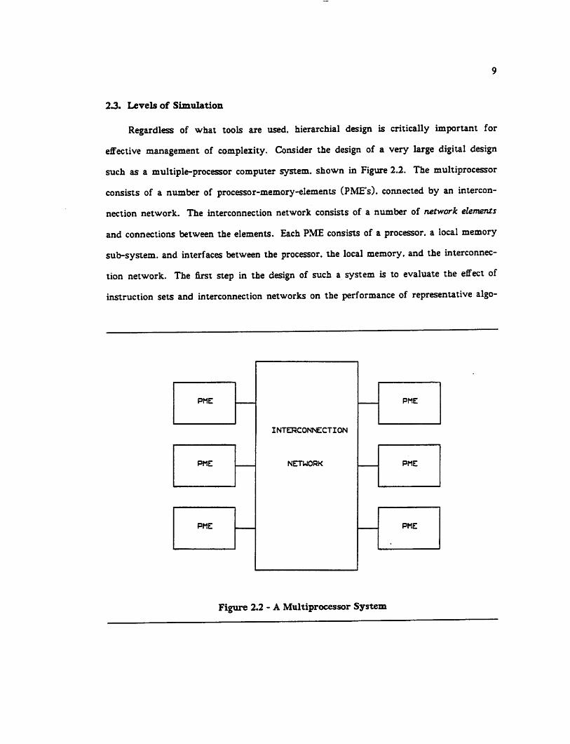
Regardless of what tools are used, hierarchial design is critically important for
effective management of complexity. Consider the design of a very large digiul design
such as a multiple-processor computer system, shown in Figure 2.2. The multiprocessor
consists of a number of processor-memory-elements (PME's). connected by an intercon
nection network. The interconnection network consists of a number of network elements
and connections between the elements. Each PME consists of a processor, a local memory
sub-system, and interfaces between the processor, the local memory, and the interconnec
tion network. The first step in the design of such a system is to evaluate the effect of
instruction sets and interconnection networks on the performance of representative algo-
INTERCONNECTION
NETWORK
PME PME
PME PME
PME PME
Figure 2.2 - A Multiprocessor System

10
rithms. A first-order understanding of the effect of these choices on system performance
can be obtained by using a behavioral-level simulation system such as GPSS [19] ADLIB
[20] or FTL2 [21]. The model of the system used at this point is purely algorithmic: no
choices as to system structure need be made, and the relative performance of the different
processes may not even be known. A behavioral-level simulation of a system aids a
designer in reasoning about critical resources, such as register files, busses, and data-paths.
The next step in the design cycle is to examine alternative structures for the system at the
large-block digital level. All levels below the functional level are considered to be struc
tural or schematic views [2] and can be represented by a schematic diagram. At this level
of abstraction, a Register-Transfer Level (RTL) simulator can be of help. Sucha simulator
allows the designer to examine the performance of different building-block configurations
under simulated input or test vectors. If the building blocks used in the RTL simulation
represent cells from a standard library this may be the lowest level of abstraction the
designer encounters. However, if any of the blocks must themselves be designed out of
lower-level components, the design parameters associated with them must be viewed as
approximate estimates or goals, and the job of the designer at the next lower level of
abstraction is to makecircuit design tradeoffs to best implement the block. The goal of the
logic design phase is to implement the building-blocks as efficiently as possible. Of course,
the choices made in the architectural phase are influenced by the structures the logic can
implement. At the logic level, the choices are between design styles with different power
and area requirements. If the primitives used are simple standard cells, this is the final
stage of the design cycle. However, in a full custom design, the designer must implement
the block functions out of more primitive elements. Here the tradeoffs become more com
plex, and aspects of the fabrication process and its parasitics must be taken into account
for high-performance design.
If there are clear Figures of Merit for the pieces of a design, then the design choice can
be analyzed in terms of those characteristics and its quality can quickly be determined.

11
High-Performance simulation is important because it allows the quality of a proposed
implementation to be determined quickly and compared to other choices. The speed of a
simulation facility effects directly the number of alternative designs a designer or program
can evaluate.
2.4. Special-Purpose Hardware for simulation
Although simulation is a powerful took for analyzing design tradeoffs, it requires
large amounts ofcomputer time to simulate large blocks orsmall blocks at high degrees of
accuracy. It is always possible to decrease the time necessary to simulate a circuit by the
use of a higher level of simulation, in many cases, however, the higher level simulation
will not capture the information which isof interest. For this reason, there is great deal of
interest in hardware solutions to the simulation problem. These simulation accelerators
can perform simulations at much greater speed than software based simulators. However,
there is a tradeoff between cost, accuracy, degree of specialization, and performance. The
tradeoff are similar those made in software simulators. [22], but the benefits and penalties
of specialization are in general far greater than in software because of the comparative
difficulty of designing and modifying hardware. Because of this difficulty, almost all work
in special-purpose hardware forsimulation has been limited to logic level simulation.
2.4.1. The Yorktown Simulation Engine
The first logic simulation machine to be reported in the open literature was the York-
town Simulation Engine, or YSE [23]. IBM has also reported an earlier effort, the LSM
[24], which contributed many ideas to YSE project, and a follow-on version, the EVE [25].
A YSE can be configured with from 1 to 256 logic processors. A block diagram of the YSE
is shown in Figure 2.3 [23].
Each logic processor can simulate up to 8192 gates at 80ns each, or 12.5 million gate-
evaluations/second. Thus, a 256 processor system would be able to simulate 2 million

INTEFl-PROCESSOR SWITCH
jn 11 1L L L A / i
0 0 0 R FI
G G G R FI
I I I A i i
C C C Y \ tto/frota
P P P P 1» hose
R R R R 1I computer
> 10 0 0 0 (
<: i: C C i
9^ ^ v Y CTRLPROC
Figure 23 - The YSE
12
gates at over 2 billion gate-evaluations/second. To put this in perspective, consider that a
good software logic simulator runs at 1000-2000 gate-evaluations/second [15] on a VAX-
11/780 Unix system. In this case, the YSE is over 1.000.000 times faster than a software
simulator but is limitied to this one function.
Every module in a YSE is driven from a central 80ns clock, and the logic processors
are connected together by 256x256x3 bit cross-bar switch. The YSE provides three state
logic simulation and all paths, including the switch, have parity. Each logic processor
sists of three parts: a 8k X 128 bit instruction memory, a 8k X 2 bit data memory, and
logic evaluation unit. Ablock diagram of aYSE processor is shown in Figure 2.4 [26].
Each instruction specifies a single four-input, single output logic function, where the
inputs and output may be modified by a mapping function, called a GDM. Note that a sin
gle output may feed any number of inputs, and that the output isnamed implicitly by the
instruction number. Each processor starts at location 0 and goes through its entire
con-
a

ean> coot
aoKi eaot
irr*a uu
or i
I I
!7 r*5 ••" » M \T'V ' *
Oat* OMt
AMr o.'
IfcMr t..tl fraction «*• <«« « "
mm out
.to uu aMar*i
M4r M«r0.1 I •>
Figure 2.4 - A YSE Logic Processor
13
instruction memory in sequence. There are no branches, conditionals, orother flow control
operations.
The YSE can operate in two modes. The first mode, unit-delay, simulates an entire
machine for a single cycle, allowing storage. The second mode, rank-order simulation,
simulates an entire block of logic between two registers in a single operation. In rank-order
simulation, it is necessary to order the logic instructions on all processors such that the
results are produced long enough before they are used so that all inputs will be available
to evaluate a logic function. In unit-delay mode, gates may be evaluated in any order, as
long as all gates in a block are evaluated before the next simulation cycle. The YSE can
also perform RTL-level simulation through the use of virtual logic. In this mode. Boolean
expressions are compiled from an RTL level simulation language into a network of four
14
input functions unlimited fanout functions. In experiments at IBM. the use of virtual
logic resulted in an average 4-to-l reduction in gate count and simulation time [27] com
pared to the standard logic-level simulation. Aswitch-level [5] MOS simulator has been
also implemented on the YSE. However, the lack of conditional execution of YSE instruc
tion has limited the efficiency of this level of simulation. A sequential fault simulator has
been implemented on the YSE as well.
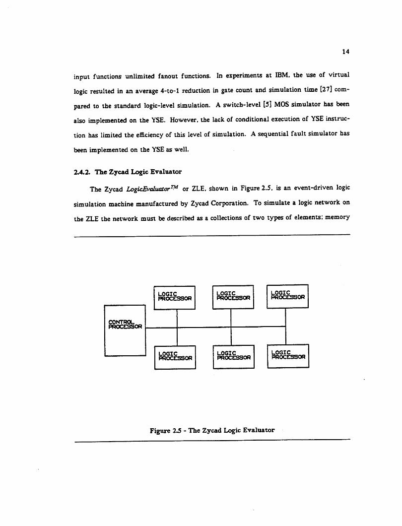
2.4.2. The Zycad Logic Evaluator
The Zycad LogicEvaluator7^ or ZLE. shown in Figure 2.5. is an event-driven logic
simulation machine manufactured by Zycad Corporation. To simulate a logic network on
the ZLE the network must be described as a collections of two types of elements: memory
CONTROLPROCESSOR
LOGICPROCESSOR
LOGICPROCESSOR
LOGICPROCESSOR
LOGIC _PROCESSOR
logic; „PROCESSOR
PROCESSOR
Figure 2.5 - The Zycad Logic Evaluator
15
elements such as ROM. RAM and PLA's. and logic elements: three input arbitrary function
gates. The simulation is a based on a three strength, three level model so that MOS can be
simulated more accurately than on a machine such as the YSE which was designed to
simulate bipolar logic, where problems such as charge sharing do not occur. ZLE's consist
of a central control processor and from one to sixteen evaluation processors. The central
processor is responsible for maintaining the central simulation clock, simulating memories
and PLA's. and providing I/O. The evaluation processors are responsible for evaluating the
three input logic gates. The central controller and all logic processors communicate over a
central 31.25 MByte/second simulation bus. Each simulation processor can hold a max
imum of 100.000 logic elements, for a total of 1.6M elements in the 16 processor system.
The ZLE is rated at a maximum of 11.4M gates/processor/second. However, published
results show a speed of 1.2M gates/second for a 5000 gate circuit. Although the ZLE can
deal more accurately with charge-sharing than the YSE. the simplifying assumptions in
logic or switch level simulators prevent them from accurately simulating dynamic circuits
and dealing accurately with charge-redistribution and noise margins. As dynamic CMOS
design styles become more prevalent, this problem may become more important [28].
2.4.3. The Daisy Megalogician
The Daisy Megalogican™ [29] is an engineering workstation consisting of a Intel
286/287 based microcomputer and a hardware accelerator for event-driven logic accelera
tion. Ablock diagram of the DML is shown in Figure 2.6 [30].
In the DML the simulation problem is partitioned into three separate tasks: queue-
management, state-processing, and evaluation. Each task executes on a separate AM2901
bit-slice machine, and the three processors are connected in a data-flow pipeline ring: The
processing cycle is as follows: The queue-manager processor dequeues the fanout-list of a
node from the time queue and issues a gate-evaluation request to the state processor for
every gate the node fans into. The state processor collects the values of the nets which

HOST
COMPUTATIONALENGINE
(80286/80287)c;
DEOICATEDMEMORY
«—*QUEUEUNIT
SYSTEM 8US
FIFO
FIFOEVALUATION
UNIT
DEDICATEDMEMORY
P
STATEUNIT
FIFO
Figure 2.6 - The Daisy Megalogician
OEO'CATED
MEWO«>
16
fanin to the gate and passes the gate type, the value's of the gate's inputs, and the fanout
list of the gate to the evaluation processor. The evaluation processor evaluates the gate
and passes the result and fanout list to the queue manager, where the process begins all
over again. User access to the Megalogician is through the Daisy simulation language
(DSL), which provides three strength, four value simulation and logic elements which
range from simple gates to fairly complex functions described by Boolean equations. The
DML has a capacity of 64K gates, and is rated at 100.000 gates evaluations/second by
Daisy (100X faster than their software running on the 286). but there are no published
benchmark results to date. From the above description, it is clear that the architecture of
the DML is distributed by function. While this approach leads to a clean partitioning of
the problem, it has the disadvantage that its performance is limited by the slowest portion
of the pipeline. One proposed way to increase the system performance of a ring architec
ture such as DML is to make several copies of the entire ring structure and connect the

17
rings by gateways which distribute the operations between the rings as described in [31].
2.4.4. The Valid RealFast
The Valid Logic Systems RealFast™. shown in Figure 2.7 [30]. is similar to the
DML. The major differences are that it uses two processors, one for event scheduling and
one for evaluation, rather than the three in the DML. The RealFast uses 32 bit data-paths
rather than the 16 bit paths in the DML. and has a 250NS cycle time, as opposed to the
DML's 500NS cycle. In addition. RealFast is packaged as a network server rather than a
M2 COMPUTER
68010CPU
8066(4)GRAPHICS
PLOT
MULTIBlJS
MAINMEMORY
EVALUATIONENGINE
EVALUATION MEMORY• 64 BITS WIDE• 32 MEGABYTES (MAXIMUM)
REALFAST SIMULATION SYSTEM
REALFAST
INTERFACE
DISKMEMORY
EVENTENGINE
EVENT MEMORY• 64 BITS WIOE• 32 MEGABYTES (MAXIMUM)
Figure 2.7 - The Valid RealFast
18
workstation. Maximum capacity of the RealFast is given as 1M elements, which translates
into approximately 2.5M gates. The result of wider data paths and higher clock speed lead
Valid to rate it at a maximum speed of 500.000 events/second as opposed to the DML's
100.000. However, there are no independent published benchmarks at this time.
2.5. Tradeoffs between general and special hardware
Although the YSE and ZLE can perform logic simulation at high speed, they are very
inflexible. The YSE. for example, can only be programmed by creating a network of logic
gates which when evaluated will give the desired results. While this method bears some
resemblance to the data-flow model of computation [17]. it represents a very restricted
subset of the model, which does not even provide conditionals! The DML. and RealFast
may be more flexible, since they are based on bit-slice technology, but this flexibility is not
currently available at the user level.
2.6. Circuit Simulation
The YSE. ZLE. Megalogican. and RealFast can improve greatly the speed of logic
simulation. However, for high performance design, logic simulation is not accurate
enough, and true circuit simulation, which these machines cannot provide, must be used.
Only circuit simulation can provide guarantee accuracy for arbitrary circuit designs.
Standard circuit simulation programs programs such as SPICE2 [32], ASTAP [33], or
ASPEC [34] solve the first-order non-linear ordinary differential equations which describe
the behavior of circuits using stiffly-stable integration methods, damped Newton-Raphson
iteration, and LU factorization. These techniques are only limited in their accuracy by the
accuracy of the device models, the detail with which the parasitics of the interconnect are
extracted [35] and the precision of the floating-point arithmetic of the computer used to
perform the simulation. Aflow diagram for a "second generation" circuit simulation pro
gram such as SPICE2 is given in Figure 2.8.

CUTTXICSTEP*•»
•LBCTHEWTIME
i•1IIIHJWTC
CLDCHTO
-UECH
BOUffTXCHB
Figure 2.8 - Circuit Simulation Algorithm
19
20
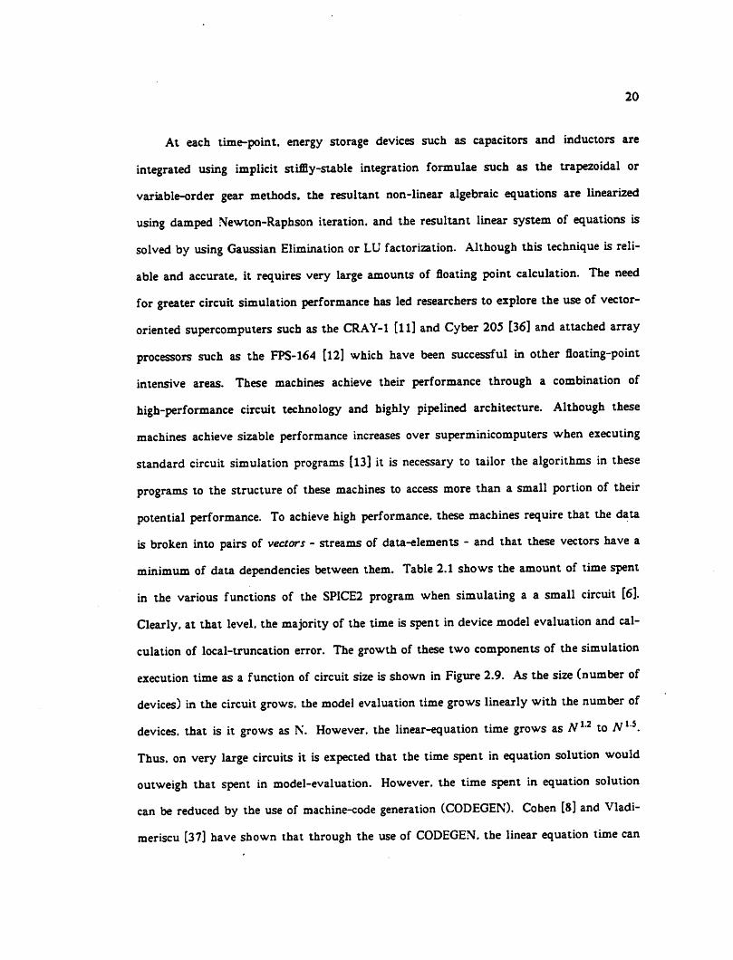
At each time-point, energy storage devices such as capacitors and inductors are
integrated using implicit stiffly-stable integration formulae such as the trapezoidal or
variable-order gear methods, the resultant non-linear algebraic equations are linearized
using damped Newton-Raphson iteration, and the resultant linear system of equations is
solved by using Gaussian Elimination or LU factorization. Although this technique is reli
able and accurate, it requires very large amounts of floating point calculation. The need
for greater circuit simulation performance has led researchers to explore the use of vector-
oriented supercomputers such as the CRAY-1 [ll] and Cyber 205 [36] and attached array
processors such as the FPS-164 [12] which have been successful in other floating-point
intensive areas. These machines achieve their performance through a combination of
high-performance circuit technology and highly pipelined architecture. Although these
machines achieve sizable performance increases over superminicomputers when executing
standard circuit simulation programs [13] it is necessary to tailor the algorithms in these
programs to the structure of these machines to access more than a small portion of their
potential performance. To achieve high performance, these machines require that the data
is broken into pairs of vectors - streams of data-elements - and that these vectors have a
minimum of data dependencies between them. Table 2.1 shows the amount of time spent
in the various functions of the SPICE2 program when simulating a a small circuit [6].
Clearly, at that level, the majority of the time isspent in device model evaluation and cal
culation of local-truncation error. The growth of these two components of the simulation
execution time as a function of circuit size is shown in Figure 2.9. As the size (number of
devices) in the circuit grows, the model evaluation time grows linearly with the number of
devices, that is it grows as N. However, the linear-equation time grows as N12 to N15.
Thus, on very large circuits it is expected that the time spent in equation solution would
outweigh that spent in model-evaluation. However, the time spent in equation solution
can be reduced by the use of machine-code generation (CODEGEN). Cohen [8] and Vladi-
meriscu [37] have shown that through the use of CODEGEN. the linear equation time can

Function
Model evaluationTruncation-error Estimation
Integration of Capacitor CurrentsLinear Equation SolutionI/O & other
Table 2.1 - SPICE2 Profile
Time
60%
20%
10%
7%
3%
21

10 10" 10'
NUMBER OF CIRCUIT EQUATIONS
Figure 2.9 - Form and solve growth Rates
22
be kept down to a small portion of the total simulation time for circuits up to 1000 nodes.
In logic simulation. I/O can take up a considerable amount of the simulation time. How
ever, in circuit simulation. I/O time tends to be negligible compared to simulation time
because to the greater complexity of circuit node processing.
23
2.6.1. Model Evaluation
For moderate sized circuits, or when machine-code solution of the linear systems is
used, model evaluation can consume a considerable part of the total simulator execution
time. In a program like SPICE2. there are three phases to the model evaluation process.
First, the model parameters and terminal voltages must be gathered from the parameter-
block and matrix. Second the model must be evaluated under the given parameters and
terminal voltages. Finally, the currents and conductances must be scattered out into the
circuit matrix. To execute model-evaluation on a vector machine efficiently, the model-
evaluation problem must be re-cast into a vector form. For example, in the CLASSIE pro
gram [37], as each class of sub-circuit is solved, all corresponding transistors in the sub-
circuit instances are evaluated by using vectorized gather and scatter operations. However,
because there are multiple paths through the model-evaluation function, and it may not be
possible to evaluate the region of operation of the model until the model has been at least
partially evaluated, models are evaluated for all operating conditions and the value from
the correct region of operation for each model is chosen after all models have been
evaluated. The result is that the time gained by vectorizing the core of model evaluation is
mostly lost due to the extra work involved in evaluating the device for all regions of
operation. Using these techniques it has been possible to improve the performance of vec
tor machines for the circuit simulation problem, but the maximum speedup achieved has
been less than an order of magnitude (usually a factor of 3 or 4) for practical circuits.
2.7. Linear Equation Solution
Conventional circuit simulation programs such as SPICE2 must solve a sparse set of
linear equations at each instant of simulated time during non-linear time-domain transient
analysis. Many other engineering problems, such as finite-element analysis and semicon
ductor device simulation, also require the solution of sparse linear systems.

24
Although vector machines can be perform operations on dense matrices with great
efficiency, the time necessary to gather sparse-matrix elements into a vector and then
scatter the result of a computation back into the matrix limit can quickly dominate the
timespent in the pipe. As mentioned above, to achieve the greatest performance on a vec
tor machine, it is necessary to provide the pipelines with long streams of data on which
identical operations can be performed. While the operations for performing Gaussian elim
ination or LU factorization [38] on dense or banded [39] matrices can be written this way.
It is much more difficult to efficiently utilize vector hardware when solving the sparse
linear systems [13] which occur in circuit simulation. One way to achieve performance
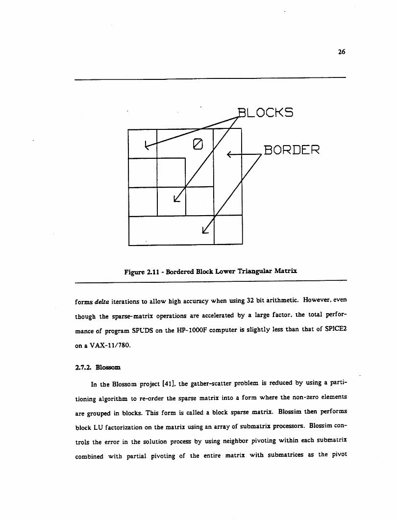
gains from vectorization of equation solution is by re-ordering the equations into bordered
block diagonal (BBD) or bordered block lower triangle (BBLT) form [10. 37. 40] shown in
Figure 2.10 and Figure 2.11 respectively. In a BBDF-based program, each of the cells in
the circuit is described by its own matrix, and the connections between the subcircuits is
given by entries in the bottom row and rightmost column. While this approach can be
useful for circuits made up of repeated cells, the regularity of the blocks along the diago
nal and the size of the borders can strongly affect the degree of speedup possible using this
technique. It is also not effective for small circuits where there is little repeated structure.
2.7.1. Special-Purpose Microcode
In some cases, cost/performance is as important as absolute performance. For this
reason. Cohen [8] has explored the use of special microcode and single-precision arithmetic
in the circuit simulation program SPUDS (Simulation Program on a pi-programmable data
system). The SPUDS program accelerates the processes of LU factorization, forward elimi
nation and back substitution through the use of special purpose microcode. By adding
only four special operations to the instruction set of a general purpose minicomputer, pro
gram SPUDS speeds up the sparse matrix operations by a factor of 20. Because of the
expense of extended precision arithmetic, program SPUDS uses an error matrix and per-

DIAGONALLOCKS
BORDER
Figure 2.10 - Bordered Block Diagonal Matrix
25
26
LOCKS
BORDER
Figure 2.11 - Bordered Block Lower Triangular Matrix
formsdelta iterations to allow high accuracy when using 32 bit arithmetic. However, even
though the sparse-matrix operations are accelerated by a large factor, the total perfor
mance of program SPUDS on the HP-1000F computer is slightly less than that of SPICE2
onaVAX-11/780.
2.7.2. Blossom
In the Blossom project [41], the gather-scatter problem is reduced by using a parti
tioning algorithm to re-order the sparse matrix into a form where the non-zero elements
are grouped in blocks. This form is called a block sparse matrix. Blossim then performs
block LU factorization on the matrix using an array of submatrix processors. Blossim con
trols the error in the solution process by using neighbor pivoting within each submatrix
combined with partial pivoting of the entire matrix with submatrices as the pivot
27
elements. Although it is possible that such an array could be coupled with model evalua
tion units and used for circuit simulation, it is currently oriented towards the solution of
general large sparse linear systems.
2.8. Kieckhafer Sparse Matrix Array Processor
Another approach to the sparse matrix problem has been reported in [42]. Here, the
gather-scatter problem is reduced by using a an associative memory to match all of the
elements with the same column number together. Linearization of the device models in
this system is achieved by the use of a arrayof processors with local interconnect.
2.9. Advanced Circuit Simulation Algorithms
All of the efforts mentioned above have focused on speeding up the direct methods
used in classic circuit simulation programs. However, while such techniques can achieve
higher performance than the same algorithms on conventional machines, algorithmic
improvements can yield far greater speedup. For example, only a few of the elements in a
large digital circuit switch at any given time. Both accurate circuit and approximate circuit
simulators called timing simulators have been developed which exploit this fact to achieve
performance enhancement. The MOTIS1 program [43] developed at Bell Labs, was a tim
ing simulator which used table-lookup MOS models and approximated the solution of the
linear equations with asingle Gauss-Jacobi iteration. Programs RELAX1[44] and RELAX2
[45] use waveform relaxation [l] techniques to decompose a circuit into subcircuits. and
allow each subcircuit to choose its own time-steps. Programs SPLICE1 [14] and SPLICE2
[15] use iterated timing analysis (ITA) [14] to accurately solve the circuit equations.
The starting point for a description of ITA is the electrical circuit equation formula
tion. Under the assumptions [l] given below:
1. All resistive elements, including active devices such asMOSFETS. are characterized by constitutive equations wherevoltages are the controlling variables and currents are thecontrolled variables.

2. All energystorageelements are two-terminal,possibly nonlinear, voltage-controlled capacitors.
3. All independent voltage sources have one terminal connectedto ground or can be transformed into independent currentsources with the use of the Norton transformation.
28
the nodal network equations, where there are N equations in N unknown node voltages.
N+l nodes in the circuit, and node N +1 is the reference node, or ground, can be written:
C(v.u h> - -f(v.u ) (2.1)
W0J = V.
where v (t ) is the vector of node voltages at time t. v (t J is the vector of time derivatives
of v {t ).u(t ) is the input vector at time t. C(• ) represents the nodal capacitance matrix.
/ . and:
f(v(t ),u(t ))-[f i(v(t ),u(t )), ••• ,fN(v(t ),u(t ))]r
where fi(v(t ),u(t )) is the sum of the currents charging the capacitors connected to
node i. The differential equations are converted to a set of nonlinear, algebraic difference
equations using a stiffly-stable integration formula to give:
«(*) - 0 (2-2>where xN is the vector of node voltages at time r„ . lt and an iterative relaxation method
(Gauss-Jacobi or Gauss-Seidel) is then used to solve them. However, unlike classical tim
ing analysis [43] where a single relaxation iteration is used per time-point, in the ITA
approach the relaxation process is continued to convergence at a time-point and the exact
solution of the system is obtained.
Only one Newton-Raphson iteration is used to approximate the solution of each nodal
equation per relaxation iteration and the evaluation of the equations is event-driven to
exploit latency. This technique, known as selective trace, traces the path of the signals
through theactive portions of the circuit, eliminating the need to process inactive elements.
29
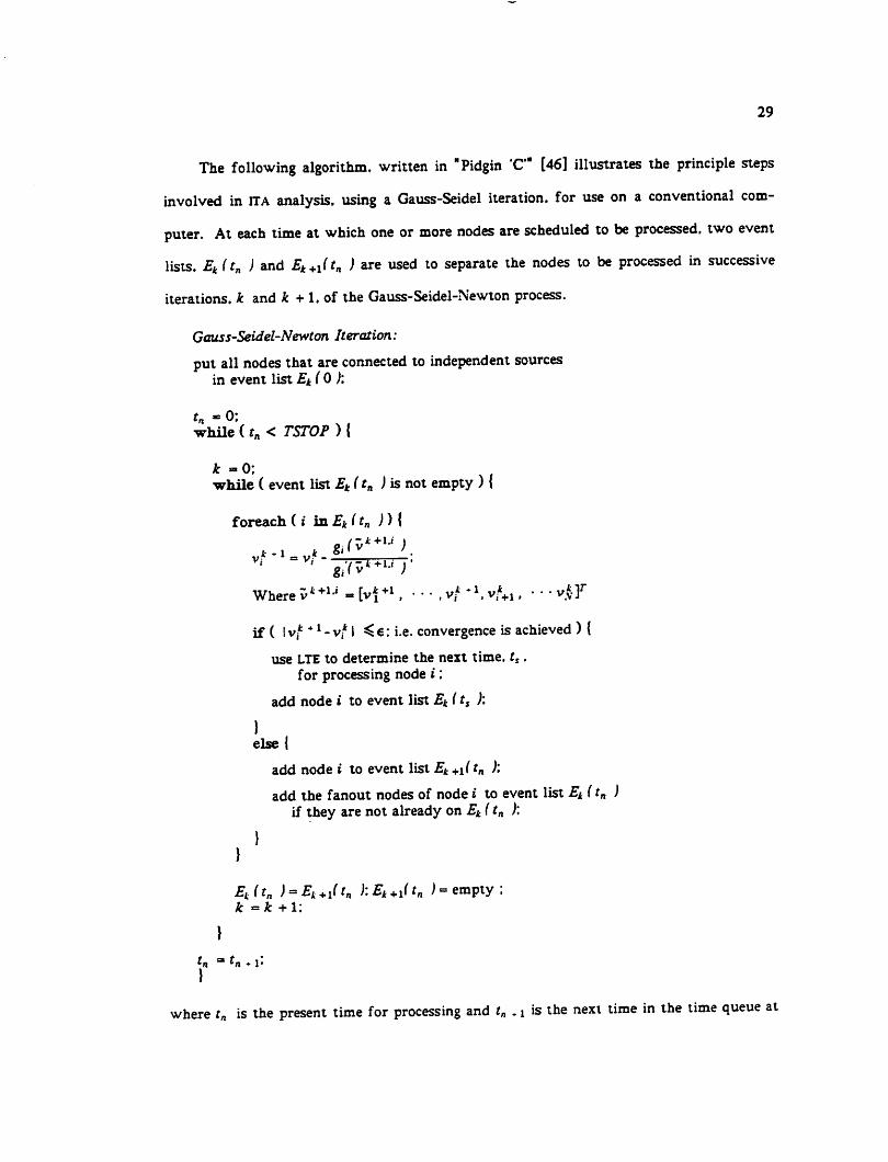
The following algorithm, written in "Pidgin C [46] illustrates the principle steps
involved in ITA analysis, using a Gauss-Seidel iteration, for use on a conventional com
puter. At each time at which one or more nodes are scheduled to be processed, two event
lists. Ek(tn ) and Ek+1(tn ) are used to separate the nodes to be processed in successive
iterations, k and k + 1. of the Gauss-Seidel-Newton process.
Gauss-Seidel-Newton Iteration:
put all nodes that are connected to independent sourcesin event list Ek (0 ):
while (tn< TSTOP ) {
k -0;while ( event list Ek (tn )\s not empty ) {
foreach (i inEk (t„ )) {
k - 1 * 8« •gi(vk )
Wherev^-M*1. ••• . v,* -1. vf+1, • ••v,vF
if ( Iv* *l - v* I ^€: i.e. convergence is achieved ) {
use LTE to determine the next time. ts.for processing node i'.
add node i to event list Ek (ts ):
}else {
add node t to event list Ek+i(tn ):
add the fanout nodes of node i to event list Ek (t„ )if they are not already on Ek (tn h
}}
Ekitn )<*Ek+i(tn ):Ek+i(tn j» empty:k =* +1:
}
}
where tn is the present time for processing and t„ , i is the next time in the time queue at

30
which an event was scheduled. In this way. the "time-step" is handled independently for
each node. The foreach construct requires that the block be executed for each member of
the set in a specified order.
This simplified algorithm does not illustrate how such issues as time-step reduction
and local truncation-error estimation are handled. These and other important details of
the algorithm are described elsewhere [15]. While a nodal formulation was used to
describe the approach, a modified nodal formulation [38] can also be derived.
The use of independent time-steps for different subcircuits and the ability to exploit
temporal sparsity are the major factors responsible for the speedups which can be achieved
using these techniques on a uniprocessor. However, while the speedups provided relaxa
tion techniques can be large for loosely-coupled circuits [l], for tightly coupled circuits or
circuits with many parasitic elements present the slower convergence rate of relaxation
methods as compared to direct methods may result in longer execution times than conven
tional circuit simulators [47]. In these cases, it can be advantageous to solve tightly cou
pled blocks by direct methods and apply relaxation between the tightly coupled blocks.
The decoupled nature of relaxation methods results in less of a need for communication
and synchronization than is required for parallel implementation of direct methods [48].
This makes them more suitable for multiprocessor implementation, as described in later
chapters of this dissertation.

CHAPTER 3
MULTIPROCESSOR ARCHITECTURE
3.1. Introduction
Multiprocessors are denned in [49] as computer systems with more than one control unit
and more than one execution unit. For the purpose of this dissertation, a more narrow
definition will be used. A multiprocessor will be defined as a system consisting of
processor-memory elements, connected by an interconnection network. The purpose of
this chapter is to review previous work in computer architecture with emphasis on its
application to circuit simulation.
3.2. Array and Vector Processors
The most common examples of multiple execution unit machines are array and vector
processors. These machines have asingle central control unit and multiple execution units.
and are also known as single instruction/multiple data (SIMD) parallel processors.
3.2.1. The ILLIAC IV
The ILLIAC-IV [50] was the first array processor. It was designed to have four qua
drants each quadrant consisting of an 8 x 8 array of processing elements, sharing a single
control unit and connected by a network consisting of connections from each execution
unit to both its nearest neighbors and its neighbors y/W away. Only a single quadrant of
the ILLIAC was built. The ILLIAC-IV. although an interesting machine, suffered from
both architectural limitations and severe reliability problems. The interconnection net
work required many cycles to be spent permuting the data for each cycle spent in program
execution. Thus, only a small fraction of the machine's possible performance was
31

32
available for all but the most fortuitous structured problems. The reliability problems in
ILLIAC IV were partially due to the use of new and untested technology. In addition, the
machine was not designed with ease of repair asa design goal. The result was a mean time
between failures (MTBF) of 10 minutes and a mean time to repair (MTTR) of 6 hours
[51]!
3.2.2. ThelCL-DAP
The DAP [52] is a modern SIMD machine which consists of a 64x64 array of single
bit processing elements (PE's) connected by a nearest-neighbor network. In addition, each
PE is connected to a bus for its row and its column, under the direction of a central con
troller. The DAP is mapped into the CPU's address space and viewed by the CPU as smart
memory rather than being connected by a channel or a co-processor interface, thus opera
tions can be performed with very low latency. Each processing element contains an ALU.
three registers. Register A is called the activity register, and is used for data-dependent
operations, register Q is a one-bit accumulator, and register C is a carry register used for
multiple-bit arithmetic. The ALU can perform any arithmetic or logical operation between
two bits, one coming from an internal register or one of the four neighbors or the row bus.
and the other coming from an internal register. The result of an operation can be stored
into a local 4K by 1 memory, or fed back into the ALU.
3.2.3. The Goodyear MPP
The MPP [53] is a large-scale SIMD machine designed mainly for image processing
applications. The architecture of the MPP is designed to allow machines to be constructed
with up to 213 single-bit processing elements, connected by a nearest-neighbor network.
The processing elements are packaged eight to a chip. Early experience of the MPP on
image processing applications has been promising. On problems such as fast Fourier
transforms of large binary images the MPP can achieve very high efficiencies. Single bit

33
machines offer great promise for image processing applications and problems such as Lee-
Moore routing [54] and bit-map based design rule checking [55], but because their architec
ture is not well suited to floating-point computations they do not at this time appear suit
able for applications such as circuit simulation.
33. Vector processors
Most digital systems can be viewed as finite state machines. In such systems, the
minimum clock cycle is determined by the longest path from a primary input or the out
put of a register through a path of combinational logic plus the set-up time of the register
it feeds into, viz: C » SRC* +LOGICrnfl +OREGT. In pipelining, long paths of combi-pa p« wup
national logic are broken up into shorter sections connected by registers. After this is
done, the clock cycle need only be long enough for the longest remaining path:
Csmauer = SRCr +PLOGICT?d +OREGTsaup. However, the cost of this approach is an
increase in the time necessary to generate the first result. Almost all modern computers
use pipelining to speedup the processing of instructions. For example, it is common to
pipeline the fetch-decode-execute cycle. Vector processors are computers which use pipe
lined ALUs, adders, multipliers, or other functional units to decrease the length of the
critical paths in these modules. They then make it possible for users to take advantage of
the pipelined structure of the functional units by providing operations on vectors of data.
The Cray-1 [ll] is perhaps the most well known of such machines, but the first commer
cial machine available with this feature was the CDC STAR-100 [56] and there are now
many machines which provide this facility.
33.1. The Cray-1
In the Cray-1. it is possible for the compiler or assembly-language programmer to
request operations between vectors of data-items. In this way. the pipelining is made
explicit, and accessible at the user level. The Cray-1 is also one of the world's fastest
scalar processors, with a basic clock cycle of 9.5ns for the current model. The original
34
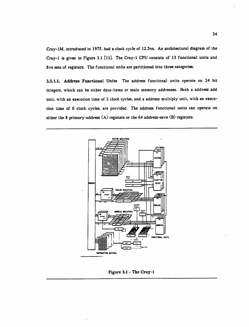
Cray-IM. introduced in 1975. had a clock cycleof 12.5ns. An architectural diagramof the
Cray-1 is given in Figure 3.1 [ll]. The Cray-1 CPU consists of 13 functional units and
five sets of registers. The functional units are partitioned into three categories.
33.1.1. Address Functional Units The address functional units operate on 24 bit
integers, which can be either data-items or main memory addresses. Both a address add
unit, with an execution time of 2 clock cycles, and a address multiply unit, with an execu
tion time of 6 clock cycles, are provided. The address functional units can operate on
either the 8 primary-address (A) registers or the 64 address-save (B) registers.
VCCTQI tfCISTMS
rUNCTIOMU. UNITS
tasnucTtoa wm«$
Figure 3.1 - The Cray-1
35
33.1.2. Scalar Functional Units The Cray-1 has 4 scalar functional units. The scalar
add unit requires 3 clock cycles to produce a result. The scalar shift unit requires 2 for a
single word shift and 3 for a double word shift. The scalar logical unit requires 1 clock
cycle. And the population-count / leading zero count unit requires 3 cycles. All scalar
functional units operate off of the 8 64 bit scalar (S) registers, and the 64 64 bit scalar-
save (T) registers.
33.13. Vector Functional Units The Cray-1 has 3 vector functional units The vector
add unit requires 3 cycles for its first result. The vector shift unit requires 4 units for its
first result. And the vector logical unit requires 2 cycles for its first result. The vector
functional units all work off of the 8 64 Word vector (V) registers. The vector multiply
and reciprocal units share circuitry with their scalar equivalents.
33.1.4. Floating-Point Functional Units The Cray-1 has 3 floating-point functional
units. The floating-point add unit requires 6 cycles to produce its first result. The
floating-point multiply unit requires 7 cycles to produce its first result. The floating-point
reciprocal unit requires 14 cycles to produce its first result. The floating-point functional
units work off both the S and V registers. Chaining is also provided between the func
tional units.
33.1.5. Cray-1 Performance If the floating-point add. multiply, and reciprocal-
approximation The original (12.5ns) Cray-1 was rated at a maximum performance of 240
MFLOPS. In actual practice the performance seen is much lower, and averages around
20-30 MFLOPS.
33.2. TheCyber-205
The Cyber-205 [36] is also vector processor. However, the tradeoffs made in its
design were very different than those in the Cray-1 The Cyber-205 has a memory to
memory vector architecture, as opposed to the register to register architecture of the

36
Cray-1. The advantage of the approach used in the Cyber-205 is that vectors of any
length may be operated on without regard to register size. However, there are many pipe
line delays involved in accessing the global memory. For this reason, the crossover point
between scalar and vector mode in the 205 is much higher than that in the Cray-1. Thus,
the Cray-1 tends to perform better on programs with shorter vectors and the Cyber on
machines with longer ones. The Cyber is also a more complicated machine. It used micro-
coded as opposed to hard-logic control, and supports both 32 and 64 bit arithmetic. The
205 has a more complicated architecture than the Cray-1 and the more dense logic is used
to implement it. It has a slower clock cycle than the Cray. 20ns vs. 12.5ns in the Cray-1
and 9.5ns in the Cray-lS.
333. TheFPS-164
The FPS-164 [12] is an attached processor which connects to a host by way of a
high-speed channel. The FPS-164 is designed to offload computationally intensive tasks
from the host and execute the at high speeds, without having to support a complicated
operating system and a large number of programming languages. The FPS-164 has a single
adder and a single multiplier, each of which is pipelined and able of accepting a new set of
operands every 167ns with a 2 stage adder and a three stage multiplier three. The prob
lems with this architecture are that it can only achieve its maximum 6 MFLOPS add and 6
MFLOPS multiply rate on long vectors. Because it requires long vectors for maximum
efficiency and has no hardware to aid in solving the gather-scatter problem, the perfor
mance of the FPS-164 on circuit simulation [57] is limited to approximately 5 times the
performance of a VAX-11/780
3.4. Data-FIow and Reduction Models
Data-Flow [17] is a model of computation characterized by two basic ideas. First,
that the execution of an instruction should be determined by when the operands of the

37
instruction are available, rather than by a separate program counter. Second, that there
should be no logical central memory but that data should flow over specific paths from
where it is produced to where it is used. Since many instructions may have their operands
available at any point in time, data-flow is a naturally concurrent model of computation.
Data-flow computation are described by a directed graph where the vertices represent
functions and the edges represent data-paths. These schemas are similar in function to
petri-nets [5&] used to model computer systems. The computation is performed by the
flow of tokens which represent data-values through the graph. The actions of each vertex
are specified through a set of firing rules which specify what action should be taken when
tokens appear on the input edge(s) of a vertex. Data-flow principles may be applied in a
wide range of areas. For example, almost all modern optimizing compilers perform some
degree of data-flow analysis to determine information ranging from when operations can
be performed outside of loops (code hoisting) to which values should be assigned to which
registers (graph coloring) [59]. There are many modifications of the basic data-flow princi
ples which have been developed in an attempt to develop computer architectures based on
data-flow principles as their most basic level of operation.
3.4.1. Safe Data-flow
In safe data-flow [17], the firing rule for all vertices specifies that when all input
edges incident to a vertex have tokens on them, and all output edges are empty, the vertex
fires consuming all its input tokens and producing tokens on its outputs. It is possible to
show that under these firing rules the graphs are deadlock-free [17] under all patterns of
inputs.
3.4.2. The Colored Token Model
Safe data-flow has several limitations. First, it cannot handle recursion without the
ability to generate graphs at execution time. Second, because all inputs must be available

38
before any processing begins concurrency can be severely limited. Third, concurrency is
also limited by the need to pre-allocate subgraphs for all computations, even though sharp
dependencies may not be known at compile time [60]. One extension of the data-flow
model, called the colored-token model [61]. removes these limitations by coloring the tokens
with function-id. iteration count, and index numbers. This technique allows sub-graphs
to beexecuted in a reentrant fashion, much in the same way that a stack based calling con
vention allows reentrant execution of subroutines in a uniprocessor. The colored token
model has been implemented on an experimental data-flow machine [31] at the University
of Manchester.
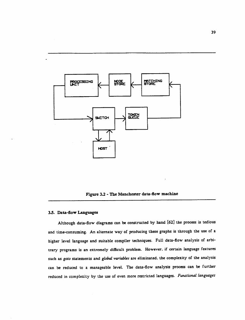
3.43. The Manchester Data-flow Machine
Ablock diagram of the Manchester data-flow machine is showing in Figure 3.2. The
heart of the machine is the matching store. The matching store is responsible for pairing
up tokens with the same color fields. When a token enters the matching store its color
field is examined. If another token with the same color is found the tokens are combined
together into an executable package If there is no other token with the same color in the
store, the token is removed from the ring and made to wait until a matching token is
found. Upon exiting the matching store, executable tokens flow into the execution unit.
The execution unit consists of a number of bit-slice based processing elements Executable
packages are passed to execution units for processing or wait until an execution unit is
available. The result of the execution of a package is one or more output tokens. If the
tokens represent output requests they are removed from the processing ring and sent to
the host. Otherwise, they are sent to the matching store and the process continues. The
only concurrency in a single-ring Manchester machine is provided by the multiple func
tional units. However, it is possible to connect multiple rings together through a switch,
and a perfect shuffle network has been proposed for this purpose.
PROCESSINGUNIT
^ SWITCH
Sul
HOST
NODESTORE
•)
£
TOKENQUEUE
MATCHINGSTORE £
Figure 3.2 - The Manchester data-flow machine
39
3.5. Data-flow Languages
Although data-flow diagrams can be constructed by hand [62] the process is tedious
and time-consuming. An alternate way of producing these graphs is through the use of a
higher level language and suitable compiler techniques. Full data-flow analysis of arbi
trary programs is an extremely difficult problem. However, if certain language features
such as goto statements and global variables are eliminated, the complexity of the analysis
can be reduced to a manageable level. The data-flow analysis process can be further
reduced in complexity by the use of even more restricted languages. Functional languages

40
[63] and Single Assignment languages allow identifiers to name values rather than storage
locations by prohibiting re-assignment to a variable. Thus statements such as "I • 1+ 1:"
are not allowed. This rule allows dau-flow analysis to be performed independently for
each module in a program by a direct symbolic execution. Several single-assignment
languages have been proposed. [64. 65]. Several of these languages support the concept of
streams of data. The stream data-type differs from standard data-flow types in that it is
permissible to begin processing the first element of the stream even if the rest of the
stream is not yet available. The SISAL language (Streams and Iteration in a Single-
Assignment Language) [65]. provides arrays, records, streams and a powerful iteration
construct which reduces the difficult in programming in a data-flow language. One advan
tage of data-flow languages and machines is that the concurrency need not be made explicit
by the programmer. All partitioning of the program is provided automatically by the
compiler and synchronization is performed as necessary by the hardware. However, such
compilers should not be viewed as a panacea: for maximum performance it is still neces
sary for the programmer to choose an algorithm with high inherent concurrency, and to
avoid adding unnecessary data-dependencies through poor implementation techniques.
3.5.1. Programming in Functional Languages
In functional programming languages, every language construct returns a value.
Identifiers in data-flow languages represent names for values, rather than storage locations.
That is. the notation ":-" represents equivalence rather than assignment. The oldest func
tional programming language is pure lisp [63]. Such languages have classically used recur
sion in place of iteration because of the difficulty of performing iteration without special
constructs or the ability to use assignment. To reduce this problem, the SISAL language
sisal provides a construct which may be used to implement many common kinds of itera
tion without having to resort to auxiliary index variables. For example, to form the sum
of the elements of an array A. the SISAL construction in Figure 3.3 could be used.

SumOfA :-FOR
tINa
RETURNSVALUE OF SUM t:
END FOR;
Figure 33 - Sum of Elements in Array
41
3.6. Implementation of ITA in SISAL
To determine the utility of a data-flow machine for circuit simulation, the ITA algo
rithm has been implemented in the ITA/DF program which is written in SISAL and exe
cutes on the Manchester data-flow machine. At the time that ITA/DF was written. SISAL
had only minimal I/O capability. To eliminate the need to implement an input processor
for ITA/DF. a preliminary version of the MSPLICE program was used to read the circuit
description and generate the SISAL data-structures which represented the circuit models,
devices and connectivity. These data-structures were then concatenated with the rest of
the ITA/DF program and the result was compiled into an executable module. The program
source for ITA/DF is included as Appendix A of this report.
At the time this work was performed, it was not practical to access the Manchester
data-flow machine remotely For this reason, as part of this research a general data-flow
graph interpreter has been developed which simulates the actions of a colored-token data
flow machine. ITA/DF was debugged by using this interpreter and then with the help of
the Computer Architecture Advanced Development Group of Digital Equipment Corpora
tion. ITA/DF was sent to the Manchester data-flow machine at Manchester England and
executed.

42
3.7. Implementation Issues
The implementation of ITA/DF exposed several interesting limitations in conven
tional dau-flow or functional languages such as SISAL. The central loop of an ITA pro
gram with selective-trace is:
1. Take the next node off the time-queue;2. Update the valueof the node by using the companion models
of its fanin elements and a single Newton step:3. Check for convergence and schedule the node and its fanout nodes
appropriately;
The algorithm given above is serial. However, if step 1 is changed to dequeue all nodes
which have new dau on their fanin nodes, a concurrent algorithm results:
1. Dequeueall nodes which are active at this iteration:For all active nodes:
2. Update the value of the node by using the companion modelsof its fanin elements and a single Newton step;
3. Check for convergence and schedule the node and its fanout nodesappropriately;
The key problems with implementing this algorithm in data-flow language involve
scheduling of nodes to be evaluated and efficient management of network state. Normally,
scheduling is through a package of procedures which modify a central time-queue data-
structure which is kept as local state inside the package. In data-flow languages, it is not
permissible for a procedure to mainuin state between executions. Thus, any "global"
data-structure must be passed by value from the main program to any routines which use
it. and those routines must return a new copy of the data-structure as part of their result.
While advanced storage management techniques may be used to reduce the amount of
physical copying that actually takes place, the result is that the time-queue must be re
generated by the inner loop of the simulator. This is true for the stream which represents
the voltages on the nodes of the circuit as well.
To reduce this problem, the SISAL language provides a construct called REPLACE
which allows a single element of an array to be replaced with a new value, the REPLACE

43
operation ukes three arguments: an array, an index, and a value, and returns an array
which is the same as the original array except that array[ index ] is replaced by value. A
natural extension of this operation might be called MULTIPLE_REPLACE. The
MULTIPLE_REPLACE operation would take an array and several {index, value} pairs as
arguments, and return a new array with those element replaced. However, no such opera
tion is currently implemented in the SISAL language and it would be difficult to add to it.
The reason is that SISAL requires that all compuutions in be deterministic, and it is
would be very difficult to determine at compile-time that a given index would never occur
more than once in the same MULTIPLEJIEPLACE operation. A general solution would be
to allow the programmer to enter into a contract with the compiler that such a conflict
would never occur, or that if it did the non-deterministic results would be accepuble. In
the ITA/DF program, the lack of a MULIPLE-REPLACE facility results in a sequential
network update phase at the end of every Gauss-Jacobi iteration.
3.8. Results
The ITA/DF program was executed on the Manchester dau-flow machine with a sin
gle NMOS inverter as a test circuit. As shown in Table 3.3. the results were extremely
good in terms of both speedup and efficiency. One of the problems encountered in the pro
gram was that the degree of concurrency available when executing the program was so
high, that when larger circuits were simulated, the number of active tokens was larger
than the matching store could hold. Because of implemenution errors in the matching
store design, it was not possible to gracefully recover from matching store overflow and
the program could not be executed on circuits larger than a single inverter.
3.9. Conclusions
The experimental implementation of ITA/DF has demonstrated that a significant
amount of concurrency is available at the fine-grain level of a relaxation-based electrical
circuit simulator. However, along with fine-grain concurrency comes the need for large

Processors Time Speedup Efficiency
1 53.1785 1.00 100.00%
2 26.5768 2.00 100.00%
3 17.7563 2.99 99.83%
4 13.3590 3.98 99.52%
5 10.7361 4.95 99.06%
6 9.0003 5.91 98.48%
7 7.7703 6.84 97.77%
8 6.8602 7.75 96.90%
9 6.1702 8.62 95.76%
10 5.6354 9.44 94.36%
11 5.2123 10.20 92.75%
12 4.8689 10.92 91.02%
13 4.5844 11.60 89.23%
Table 3.1 - ITA/DF Performance
44
amounts of communication and frequent synchronization. Because of the amount of com
munication and synchronization required, at this time, it is not clear that very large mul
tiprocessors can be built based on fine-grain data-flow principles. Because of this, a new
distributed circuit simulation algorithm Distributed Iterated Timing Analysis (DITA) has
been developed. The DITA algorithm uses dau-flow principles at the equation level,
requires much less communication than ITA/DF. and is more suiuble for use with loosely
coupled multiprocessors.
CHAPTER 4
INTERCONNECTION NETWORKS
4.1. Introduction
In a multiprocessor system such as the ones described above, each processor in the system
can reference its own local memory, buffer, or cache in the same way as a uniprocessor.
However, to reference memory on other processors, or send messages to other processors, it
must use the interconnection network. The network is a shared resource and unless the
proper design decisions are made it can limit the performance of the system.. An intercon
nection network is a structure which can implement one or more connections at any point
in time. A connection is defined as a mapping one or members of a set of inputs and one or
more members of a set of outputs. In general, a connection of more than one member of
the input set onto a single member of the output set is considered illegal. Aconnection of
a single member of the input set to more than one member of the output set is named a
broadcast. If the inputs and output sets are identical, and each member of the input set is
mapped onto one and only one of the output set. then the connection set represents a per
mutation. A network capable of performing all permuutions and broadcasts is called a
general connection network [66] or GCN.
4.2. Evaluation criteria and performance metrics
The major logical characteristics of an interconnection network are its control
category, blocking, bandwidth, latency, set-up time, switch-count, and switch complexity.
45

46
43. Network control categories
Methods for network control may be broken down into three categories [49] Synchro
nous (Centralized), re-arrangeable. and Asynchronous (or distributed). A synchronous
network is one where there is a central network controller which sets the switches in the
network. A re-arrangeable network [67] Is one where a new connection may be added to
the network by rearranging the settings of some of the switches in the network, leaving
existing connection unchanged. Synchronous networks are used in SIMD machines, where
single or multi-dimensional arrays of dau are used in a lock-step fashion. Re-arrangeable
networks are normally used as circuit switches where the connections are changed infre
quently compared to the basic cycle time of the network. These networks are popular in
telephony, where a connection may be mainuined for many millions of bit-times.
4.4. Blocking
Networks which can perform any connection in a set of connections are called non-
blocking under that set of connections. The only single-suge network which is non-
blocking under the general connection is the fully-connected graph or crossbar [49] The
Clos and Benes networks [67] are multi-suge networks which are re-arrangeable and
non-blocking under the general connection. Although the ability to be able to perform
general connections is useful for some algorithms such as matrix multiply on a SIMD
machine [50] these networks require large numbers of switches and links. Networks
which cannot perform a given connection are said to be blocking under that permutation.
Because some permuutions are more important than others in SIMD machines, there has
been a large amount of research into networks which provide small sets of very useful
permutations and into parallel algorithms which can take advantage of such networks [68]
and their properties.

47
4.5. Latency
The minimum latency of a network may be defined as the time needed for a
minimum length message entered into one port of a network to exit the network at its des
tination port. In the case of a synchronous network, the latency is normally calculated as
the clock period tc times the number of stages ns. However, a more accurate approxima
tion would be to include time necessary to calculate the setting of the switches in the the
network, which for some networks may be very long [69]. In an asynchronous packet-
switched network, the average latency of the network isa function of load of the network,
which may be defined as either the percentage of non-empty packets in the network, or the
percentage of input ports which have requests in the network, and of the destination pat
terns of the requests. Under a given statistical pattern of destination addresses (usually a
uniform distribution model) as in [6S] and a given load, the latency of an asynchronous
network is defined as the average time necessary for a message to travel from input to out
put. Although asynchronous network delay may be calculated by such techniques as Mar
kov analysis [60] accurate closed form analysis is difficult and behavioral simulation tech
niques [21] are more commonly used.
4.6. Bandwidth
The bandwidth of an interconnection network is usually defined as the rate at which
information can enter one port of the network and leave through another port. The max
imum bandwidth of a synchronous network is given by -—Xn, which is the bandwidth of
the network when sending messages of length nm » ns. There maximum bandwidth of
an asynchronous network is a function of the load on the network and the particular pat
tern of requests, and is usually determined by simulation.

48
4.7. Connection Topology
There are many different interconnection networks. A result of this research is the
realization that the "best" network is highly application dependent. However, it is
interesting to examine the major choices to determine where they sit in the design space.
4.7.1. Busses
The bus interconnection is show in Figure 4.1. For a synchronous bus with AT
processor-memory elements. A address bits. D data bits and a clock rate of C total
bandwidth is DxC bits/second, the minimum latency is -^ the maximum latency is NxC
and average maximum latency is —=— if round-robin prioritycollision resolution is used.
TOOESSOR PROCESSOR PROCESSOR
MEMORY MEMORY MEMORY
Figure 4.1 - The Bus Network

49
4.7.1.1. Cached Busses One way to reduce the load on the network in a shared-bus sys
tem is to use Dual Associator or snooping caches on the processors [70]. Figure 4.2 shows
the architecture of such a system. Each PME or other device interfaced to the bus has a
cache with two identical look-up ubles. In the Goodman Write-Once scheme. [70] each
cache has an associator for references made by the processor and a second one for refer
ences which occur on the bus. All data starts in main memory and all cache Ugs are ini
tially invalid, when a read reference is first made to physical location L by a processor X.
the location is read and the contents are entered into the cache of processor X. From that
point on. any reads directed by processor X to location L will cause its value to be
returned from cache and no traffic will be generated on the bus. If at any point, any other
processor Y attempts to read physical location L then the value of the location, which is
unchanged from its initial value, is entered into that processors cache as well and that pro
cessor has read access as well. If processor X writes into physical location L which is in
PROC. PROC. PROC. PROC.
CRCHE CRCHE CRCHE CACHE
MEMORY MEMORY MEMORY MEMORY
Figure 4.2 A Cached Bus Multiprocessor System

50
its cache, the value is written into the cache and also into main memory. If any other pro
cessors have location L in their cache, their cache entry for L is marked invalid At this
point, if any other processor Z references physical location L for read, the current value
of location L is written out onto the bus by processor X 's cache and a line is raised on the
bus saying that processor Z may not cache location L. This is a steady-state condition.
However, if at any point processor X's chooses to flush location L. it writes the current
value its entry for physical location L into main memory physical location L. From this
point on. if any processor references physical location L for read, the memory will
respond with the current value of physical memory location L. The decrease in bus traffic
that results from the use of caches is a function of the address reference patterns of the
elements connected to the bus and a strong function of references to shared writable
memory.
Electrical effects must also be considered. For any kind of interconnection structure,
the maximum signal rate for a single link an inverse function of the length of the link.
This limits the physical size of any network, but effects busses most strongly. In addition,
every element which is connected to the bus increases the busses capacitance and in the
case of bipolar logic, decreases the resisUnce to ground as well. In most current systems,
loading effects are the dominant factor limiting bus performance.
4.7.2. Ring networks
A ring connection is shown in Figure 4.3 [67]. Here, there is an active element called
a repeater at each sution. Signals are passed from repeater to repeater, and rather than
having to drive the whole length of the interconnection network as in the case of the bus.
the repeater element need onlydrive thesegment of the communications from itself to the
next repeater. Thus, large rings may be run at greater clock rates than large busses. For
example, the CDC Advanced Flexible Processor (AFP) uses an 800MB ring to connect its
functional units.

51
PME
PME
Figure 43 - A Ring Network
The bandwidth of a ring can easily be made very high, however, the latency is in
general longer than that of a bus. The maximum bandwidth of a ring is given by CxD.
The minimum latency occurs in the unusual case of each sution on the ring sending a mes
sage whose destination is the next sution on the ring. In this case, the latency experienced
by any message is -i-. Amore accurate model of the performance of the ring can be given
by simulation.
4.7.3. The Crossbar Connection
The crossbar network, shown in figure 4.4 [67], has the highest maximum perfor
mance of any of the networks described here, but also has the highest cost. Maximum
bandwidth for the crossbar is NxD. Minimum latency is 1. Maximum latency in the
absence of conflict at the memories is also 1 but conflict may occurat the memory modules
as well, reducing the performance advantage of the crossbar over the more economical net-

works.
PME
PME
PME
PME
PME
Figure 4.4 - A Crossbar Network
52
4.7.4. Nearest-neighbor networks
The two most popular nearest neighbor networks are the square and hexagonal arrays
[67] shown in Figure 4.5 and Figure 4.6. These networks have very high maximum
bandwidth, but marginal normal performance. The reason for this is the long latency
necessary to reach a remote processor. In a square nearest-neighbor matrix of N proces-
__ V2W*sors. there are ViV processors on a side. The maximum latency will therefore be —^—.

1 |PME PME PME
PME PME PME
PME PME PME
Figure 4.5 Square Nearest-Neighbor Network
53
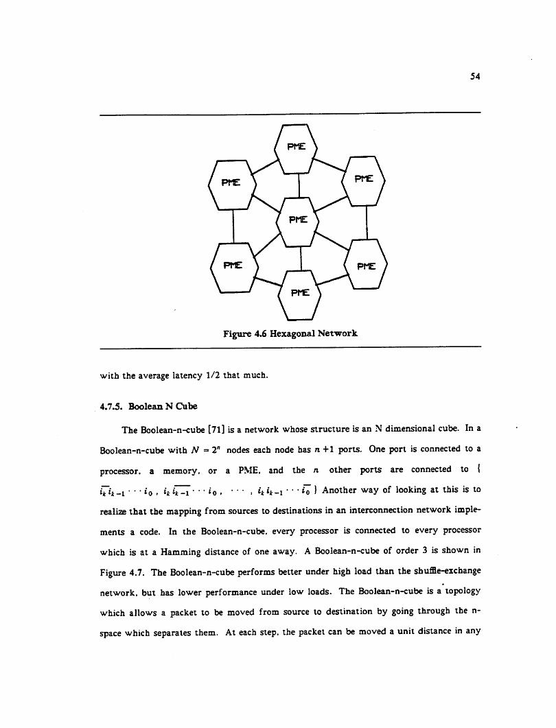
54
Figure 4.6 Hexagonal Network
with the average latency 1/2 that much.
4.7.5. Boolean N Cube
The Boolean-n-cube [71] is a network whose structure is an N dimensional cube. In a
Boolean-n-cube with N = 2" nodes each node has n +1 ports. One port is connected to a
processor, a memory, or a PME. and the n other ports are connected to {
Mi-t • ' **o . hk^i' " *o . •** , M*-i ' " ' *o I Another way of looking at this is to
realize that the mapping from sources to destinations in an interconnection network imple
ments a code. In the Boolean-n-cube. every processor is connected to every processor
which is at a Hamming distance of one away. A Boolean-n-cube of order 3 is shown in
Figure 4.7. The Boolean-n-cube performs better under high load than the shuffle-exchange
network, but has lower performance under low loads. The Boolean-n-cube is a topology
which allows a packet to be moved from source to destination by going through the n-
space which separates them. At each step, the packet can be moved a unit distance in any
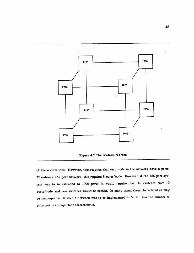
55
Figure 4.7 The Boolean-N-Cube
of the n directions. However, this requires that each node in the network have n ports.
Therefore a 256 port network, this requires 8 ports/node. However, if the 256 port sys
tem was to be extended to 1000 ports, it would require that the switches have 10
ports/node, and new switches would be needed. In many cases, these characteristics may
be unacceptable. If such a network was to be implemented in VLSI, then the number of
pins/port is an important characteristic.
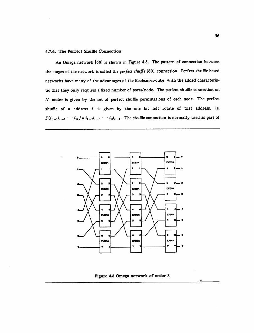
56
4.7.6. The Perfect Shuffle Connection
An Omega network [68] is shown in Figure 4.8. The pattern of connection between
the suges of the network is called the perfect shuffle [60], connection. Perfect shuffle based
networks have many of the advanuges of the Boolean-n-cube, with the added characteris
tic that they only requires a fixed number of ports/node. The perfect shuffle connection on
N nodes is given by the set of perfect shuffle permutations of each node. The perfect
shuffle of a address / is given by the one bit left rotate of that address, i.e.
S(h-ih-2 *' "l*o )~ h-2h-i ' "**o**-i- The shuffle connection is normally used as part of
e o e e
DCBOX
1 1
e 8
EXBOX
1 1i__ J—
cxbox
Figure 4.8 Omega network of order 8

57
a shuffle-exchange network. Here, the output of each shuffle suge feeds a set of exchange
boxes (2x2 crosspoints). The exchange function of an address is given by the set {
M*-i **•*o . »* **-i *' ' »"o ) In other words- the exchange box allows the lowest bit of
the address to be passed through either negated or unchanged. The shuffle-exchange com
bination can therefore be thought of as a network which takes a collection of inputs
(points in n-space) and transforms each to a a set of points which is equal to the result of
shifting the address one bit left with the lowest bit becoming a don't care. Thus it can be
seen that while the n-cube is a network which allows a packet go any direction in n-space
at any point in its travels, each suge of shuffle-exchange allows changing one bit of the
packets position in n-space. The perfect shuffle may be viewed as an indirect Boolean-n-
cube. By re-arranging the switches in the interior stages of a multiple-suge shuffle-
exchange network, it is possible to create a network which does not shift the address of
the packet each time, but where each stage is responsible for either "passing" or "comple
menting" one of the bits of the address.
4.7.6.1. The single-stage recirculating shuffle network
The shuffle connection may also be used in a configuration where a single stage is used
several times in order to move a packet from its source to destination address. The
single-suge shuffle is show in Figure 4.9. This network is similar to the n-cube in that the
processor-memory elements are connected directly to a single level of switches. Both the
Boolean-n-cube (BNC) and the single-stage recirculating shuffle (SSRS) can be thought of
as directed graphs where the vertices of the graph represent processors and the edges of the
graph represent communications ports.
4.8. Summary
The interconnection networks described above are only a sampling of the major archi
tectures. For circuit simulation and other related applications where a large number of
processors may be used, the major requirement of the network is that it have an 0 log(N)

nc 6 6
EWOX
Figure 4.9 Single-Stage Shuffle of order 8
58
asymptotic latency with the number of number of ports N. and that it supports multiple
active paths.
In practice the performance of such a network today is a much stronger function of
the node complexity and the engineering of the network (circuit technology, implementa
tion details, and electrical tradeoffs) than its purely architectural aspects. For example,
the BBN butterfly [18] uses a base-4 perfect shuffle interconnection network. Therefore.

59
the time to send a message should be log4(W ) where N is the number of ports. The remote
memory reference time for a 16 processor Butterfly is 4ms. Yet because of the width of
the dau-paths and the use of pipelining, the delay for a 128 node network is only 4.25ms.
rather than the 32ms that the asymptotic model would imply.
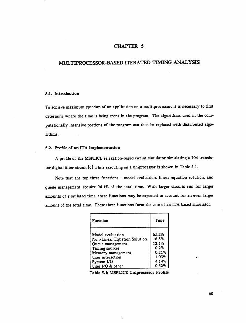
CHAPTER 5
MULTIPROCESSOR-BASED ITERATED TIMING ANALYSIS
5.1. Introduction
To achieve maximum speedup of an application on a multiprocessor, it is necessary to first
determine where the time is being spent in the program. The algorithms used in the com-
puutionally intensive portions of the program can then be replaced with distributed algo
rithms.
5.2. Profile of an ITA Implementation
A profile of the MSPLICE relaxation-based circuit simulator simulating a 704 transis
tor digital filter circuit [6] while executing on a uniprocessor is shown in Table 5.1.
Note that the top three functions - model evaluation, linear equation solution, and
queue management require 94.1% of the toul time. With larger circuits run for larger
amounts of simulated time, these functions may be expected to account for an even larger
amount of the total time. These three functions form the core of an ITA based simulator.
Function Time
Model evaluation 65.2%
Non-Linear Equation Solution 16.8%
Queue management 12.1%
Timing sources 0.2%
Memory management 0.21%
User interaction 1.03%
System I/O 4.14%
User I/O & other 0.32%
Table 5.1: MSPLICE Uniprocessor Profile
60
61
53. Processor node Architecture
As seen above, in order to achieve high performance it is necessary to provide support
'for queue manipulation, model evaluation, and convergence checking, and local truncation
error (LTE) or iteration-count [32] time-step control. Queue manipulation may be
accelerated through the use of special-purpose hardware such as bit-slice processors.
Evaluation of analytic models requires large amounts of floating-point operations, and can
be accomplished at high speed only if enough functional units and dau-paths are pro
vided. For example, an MOS model which accurately considers short-channel effects, such
a the Level-2 model in the SPICE2 program, can require over 100 floating point operations
to accurately calculate drain current and its derivatives [72] and can Uke 6ms to execute
on a VAX-11/780 class machine. Companion model evaluation time can also be reduced
through the use of uble models [6. 7]. The remaining tasks, evaluation of single linear
equations and checking convergence, can be also performed at high speeds if enough func
tional units and dau-paths are available along with a control unit capable of taking
advanUge of them.
5.4. Model Evaluation
The concurrency available in model evaluation depends on the technique used to
solve the linear equations as well. In the case of Gauss-Jabobi iteration, the voltages at the
terminals of the circuit element are given by the solution to the circuit at the previous
iteration. For Gauss-Seidel. the voltages from the current iteration are used whenever pos
sible. It ispossible to evaluate any model whose inputs are available for the current itera
tion in parallel.
53. Equation solution
The equation solution in MSPLICE is data-driven as well. When all the circuit ele
ments that the equation depends on have been evaluated and their small-signal equivalents
62
returned, the equation itself may be solved. The solution to the equations is performed in
a manner similar to data-flow [17] except that the grain of the compuution. the smallest
schedulable amount of work, is larger [73]. In distributed ITA (MSPLICE). the macro-
dataflow elements are implemented as processes.
5.6. The Scheduler
The third most time-consuming element of the ITA process is the scheduling of equa
tions to be solved. The scheduler serves two purposes. The first is to mainuin the correct
partial order of model evaluation and equation solution, the second is to control the pro
gress of the simulation clock which specifies the virtual time in the simulation run. To
bound the speedup possible in a multiprocessor implemenution of MSPLICE. it is useful to
examine the performance of MSPLICE on a set of ideal multiprocessors through simulation.
The results from these ideal models can serve to bound the speedup possible on real
machines.
5.7. The Ideal Gauss-Seidel Machine
Consider an ideal Gauss-Seidel machine. Such a machine consists of an infinitely fast
central controller, which schedules equations optimally inzero time, an infinitely fast ICN
which transmits information between equation processors in zero time, and N equation pro
cessors which can each solve an equation in a single unit of time. Note that only the
machine is optimal. For any given set of equations the order in which the equations are
solved may not be optimal. The results of simulating this machine solving an example cir
cuit are given in Table 5.2. The ideal Gauss-Seidel machine performs optimal global
assignment of nets to processors, in zero time, and has a zero delay, infinite bandwidth
network. Because it performs scheduling in zero time it gives bounds on the performance
that can be expected for simulation of the example circuit.

Processors Speedup Efficiency
1 1.00 1.00
2 1.97 0.98
3 2.92 0.97
4 3.81 0.95
5 4.80 0.96
6 5.65 0.94
7 6.51 0.93
8 7.32 0.92
9 8.08 0.90
10 8.86 0.89
11 9.56 0.87
12 10.26 0.85
13 10.93 0.84
14 11.65 0.83
15 12.28 0.82
16 12.95 0.81
32 20.46 0.64
64 28.47 0.44
128 34.18 0.27
63
Table 5.2: Ideal Gauss-Seidel Machine
Note that even an ideal multiprocessor cannot achieve 100% efficiency on this circuit-
algorithm combination. The reason for this is that this circuit is not large enough to keep
all processors busy at all times. As the nodes in the circuit converge, the system goes
through a phase where there are less active nodes than there are processors. This effect is
illustrated in Figure 5.1 which shows the activity of the test circuit for a portion of the
simulation interval. At 64 processors, a maximum 44% efficiency is possible for this exam
ple. However, if the simulation machine is multiprogrammed to simulate several circuits
concurrently the idle time can be subsuntially reduced.
The ideal model presented above is accurate only if the equation solution time is very
long relative to the time necessary to enqueue and dequeue equation events in the central
event queue, and if the network bandwidth is very high and latency is very low as well.
A more accurate performance estimate can be obtained if the network time is still set to
zero, but a finite time is charged for queue manipulation. For example, if the time neces
sary to enqueue and dequeue an equation is as large as the equation solution time itself, a
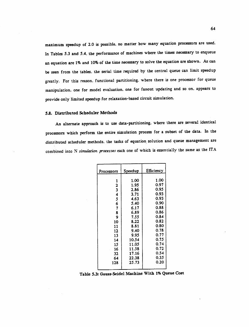
64
maximum speedup of 2.0 is possible, no matter how many equation processors are used.
In Tables 5.3 and 5.4. the performance of machines where the times necessary to enqueue
an equation are 1% and 10% of the time necessary to solve the equation are shown. As can
be seen from the tables, the serial time required by the central queue can limit speedup
greatly. For this reason, functional partitioning, where there is one processor for queue
manipulation, one for model evaluation, one for fanout updating and so on. appears to
provide only limited speedup for relaxation-based circuit simulation.
5.8. Distributed Scheduler Methods
An alternate approach is to use dau-partitioning. where there are several identical
processors which perform the entire simulation process for a subset of the dau. In the
distributed scheduler methods, the tasks of equation solution and queue management are
combined into N simulation processes each one of which is essentially the same as the ITA
Processors Speedup Efficiency
1 1.00 1.00
2 1.95 0.97
3 2.86 0.95
4 3.71 0.93
5 4.63 0.93
6 5.40 0.90
7 6.17 0.88
8 6.89 0.86
9 7.55 0.84
10 8.22 0.82
11 8.81 0.80
12 9.40 0.78
13 9.95 0.77
14 10.54 0.75
15 11.05 0.74
16 11.58 0.72
32 17.16 0.54
64 22.38 0.35
128 25.73 0.20
Table 5.3: Gauss-Seidel Machine With 1% Queue Cost

Processors Speedup Efficiency
1 1.00 1.00
2 1.81 0.90
3 2.48 0.83
4 3.04 0.76
5 3.57 0.71
6 3.97 0.66
7 4.34 0.62
8 4.65 0.58
9 4.92 0.55
10 5.17 0.52
11 5.38 0.49
12 5.57 0.46
13 5.74 0.44
14 5.92 0.42
15 6.06 0.40
16 6.21 0.39
32 7.39 0.23
64 8.14 0.13
128 8.51 0.07
65
Table 5.4: Gauss-Seidel Machine With 10% Serial Time
process described earlier. However, this creates the need to keep all of the schedulers in
loose synchronization. The schedulers must be synchronized because it is necessary to
determine the final value of a node at time Tn before beginning to determine its value for
time rn+1. It is not enough to know that a node has converged; if the inputs to the ele
ments that effect the value of the node change, the node may be re-scheduled and possibly
converge to a different value. It is only safe to go on when all the nodes which can
indirectly effect the value of the node have themselves converged. A conservative
approach to this problem is to require that all the nodes in the circuit have converged at
T„. before going on to process any of them at the next time point. In the single scheduler
method, this is guaranteed by the time ordering of the events in the single time-queue;
events for T„ are always put into the queue before events for Tn+i. In the distributed
schedule method, this is achieved by the use of a convergence-counter which keeps track of
the number of unconverged nodes in the system. Each time a node is scheduled for the
first time at a time-point, the counter is incremented and each time a node converges it is

66
decremented. When the counter reaches zero all nodes in the circuit have converged at Tn.
and simulation processes may begin processing nodes active at time Tn +i. The algorithm is
given below [16]:
foreach ( node i in M scheduled at f„ ) {
/*STEF(1):*/
foreach ( fanin element at i )obuin its fanin node voltages, vf,
) **i, K - k orfc+ 1:
/* STEP (2): */
foreach (fanin element at i )compute its contributions to nodal equation;
obuin v* *l using a single Newton-Raphson stepas described in Section 2:
if ( convergence is achieved ) {
if ( vf * v/1'l ) {
schedule i at tn . j;
}
decrement ConvergenceCounter:}else {
schedule i again at tn ;
forall ( fanout nodes of i ) {
if ( fanout node was not previously scheduled at t„ ) {increment ConvergenceCounter:
}send message to their PME to
schedule fanout node at tn ;
}
}
}
Fanin elements of node i are circuit elements (transistors, capacitors, voltage sources, logic
gates, etc.) which are used to determine the new voltage at i. as illustrated in Figure 5.1.
On average, there are ^r^ fanin elements per node. To process each fanin element, it is
necessary to obtain its controlling node, or fanin node, voltages, vf. Assume there are. on
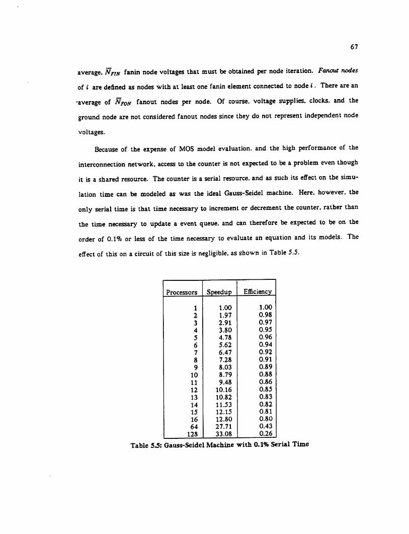
67
average. Nfin fanin node voluges that must be obuined per node iteration. Fanout nodes
of i are defined as nodes with at least one fanin element connected to node i. There are an
•average of Nfon fanout nodes per node. Of course, voltage supplies, clocks, and the
ground node are not considered fanout nodes since they do not represent independent node
voltages.
Because of the expense of MOS model evaluation, and the high performance of the
interconnection network, access to the counter is not expected to be a problem even though
it is a shared resource. The counter is a serial resource, and as such its effect on the simu
lation time can be modeled as was the ideal Gauss-Seidel machine. Here, however, the
only serial time is that time necessary to increment or decrement the counter, rather than
the time necessary to update a event queue, and can therefore be expected to be on the
order of 0.1% or less of the time necessary to evaluate an equation and its models. The
effect of this on a circuit of this size is negligible, as shown in Table 5.5.
Processors Speedup Efficiency
1 1.00 1.00
2 1.97 0.98
3 2.91 0.97
4 3.80 0.95
5 4.78 0.96
6 5.62 0.94
7 6.47 0.92
8 7.28 0.91
9 8.03 0.89
10 8.79 0.88
11 9.48 0.86
12 10.16 0.85
13 10.82 0.83
14 11.53 0.82
15 12.15 0.81
16 12.80 0.80
64 27.71 0.43
128 33.08 0.26
Table 53: Gauss-Seidel Machine with 0.1% Serial Time

68
For very large circuits, however, any serialization should be avoided. To reduce seri
alization further, it is also possible to distribute counter management as well and create a
system where there is a local counter for each of the N processes. Cm - ijv). which keeps
track of the number of unconverged nodes on that process, and a global counter NI which
gives the number of non-idle processes. The following method may be used; Every time a
process Pschedules a node to be evaluated by a process Q. P sets a lock variable. LQ which
is kept on process Q. Process P then performs an atomic increment on process Q's conver
gence counter. CQ which returns the previous value of CQ. If CQ was previously zero,
process Patomically increments NI. the global number of active processes. Process P then
clears LQ . regardless of the previous value of CQ. Every time a node converges on process
Q. process Q checks to see if LQ is set and waits for it to clear if it is. Process Q then
decrements its local convergence counter, and if the new value of the counter is zero, pro
cess Q atomically decrements NI. the count of active processes. If the count of active
processes reaches zero, the process then sends a message to all other processes, telling them
to begin processing nodes for the next time point.
At the start of a time-point Tn . NI is set equal to the number of processes in the
system, and C, for every process is set equal to the number of nodes which are currently
scheduled to be evaluated by that process. If NI is greater than one. then more than one
process is active and any action taken by a single process cannot change it to zero. If NI is
equal to one then there can be only one process. P. which has one or more unconverged
nodes, and C; for all other processes must be zero. If the convergence counter for P is
greater than one. then it cannot go to zero in a single step. If the convergence counter for P
is equal to one. then it must have one and only one active node. If the single node it is
processing converges, and if its value has changed significantly since the last time it con
verged, the process will first schedule the fanout nodes of that node, which will cause the
local counter of the process that the fanout node(s) belong to to be incremented and will
cause the global counter to become greater than one if any of the fanout nodes belong to

69
other processes. The process P will then decrement its local counter, and decrement the
global counter if the local counter has become zero. Thus, the only way the global counter
can become zero is if the last active node in the circuit at time Tn converges to a value
insignificantly different from the last value it converged to: that is. when all nodes in the
circuit have converged at time Tn .
5.9. Remote Memory Reference Models
Three levels of memory reference time modeling have been considered during this
research. The level one model specifies that all accesses to memory require one unit of
time regardless whether the reference is to local or remote memory. The level two model
specifies that references to local memory are requires one unit of time and accesses to
remote memory require Trem units. The level three model considers the effects intercon
nection network delay and memory access conflicts on remote memory access to determine
the exact memory reference time under the reference load provided by the application pro
gram. The level one model, although simple, is not accurate enough to allow any insight
to be gained into the performance of a distributed algorithm. The level-three model,
although very accurate, is very time consuming to simulate and may not provide subsun-
tially more accurate results than the simpler models depending on the characteristics of
the interconnection network being used. The level-two model is a good compromise for a
central interconnection network and memories which are dual ported to appear local to one
processor and remote to all others such as the BBN Butterfly [18] or for machines based on
a shared bus and distributed caches such as the Sequent Balance 8000 [28]. The following
is a simple analytic model of the performance of the MSPLICE algorithm using the level-
two reference model, the values of the controlling node voltages Vf will require a local
memory reference per node if the node resides on the same processor-memory element
(PME) as node i. otherwise it will require remote memory references. In the worst case,
all fanin element nodes will reside on remote PMEs and all memory references will require
70
trm units of time. Assuming only one remote memory reference can be active at any time
for a particular PME. the average time uken for Step (1). r i. can be approximated by:
tl-NFIN'rem (5-l}Step (2) does not require the processor to wait for a remote answer and hence the
time taken in Step (2) depends only on the performance of the PME. not the interconnec
tion network (ICN). The time required to solve a single nodal equation is proportional to
the number of fanin elements, since each one must be processed for the Newton-Raphson
step. In fact, the processing of each transistor. teval. dominates the PME time, with a small
amount of time. tovhd, for checking convergence, updating local memory, etc. The time
required for Step (2) can be written:
12 » hvhd +NFIEttval (5-2)For MOS or Bipolar circuits, where each transistor has three controlling terminal vol
tages. —IS -2. If supply voltages and ground are considered as special-case nodes andNfie
do not require remote reference, analysis of a number of large MOS circuits indicates that
0.5 < ^f7A' <2. Typically —— is less than 1.2 for NMOS circuits and is less than 1.5NFIE NF1E
Nfjfjfor CMOS circuits. For the example circuit -— is 1.16.
Nfie
5.10. The Unit Delay Model
The performance of the distributed scheduler algorithm can be predicted and
bounded in a similar manner to the central scheduler method. The unit delay model simu
lates processors that have their own schedulers, and are connected by a non-ideal network.
The network has a unit delay, and nodes are statically assigned to processors. Data on the
unit delay model is given in Table 5.5.
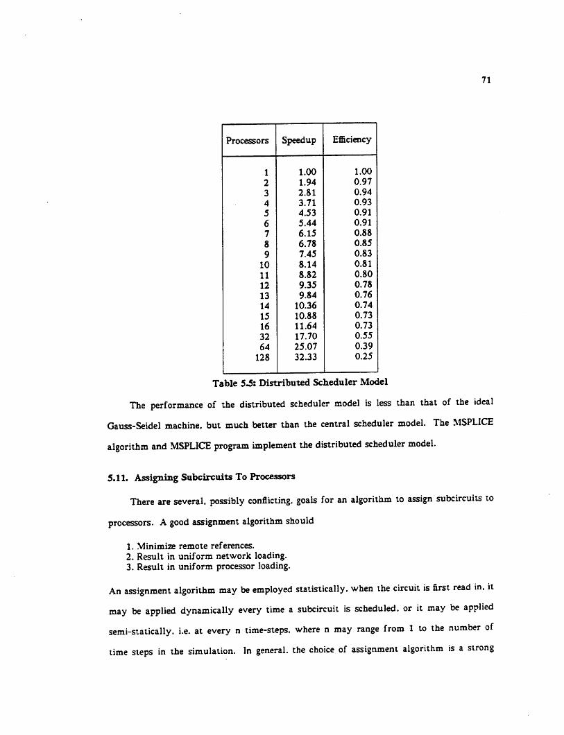
Processors Speedup Efficiency
1 1.00 1.00
2 1.94 0.97
3 2.81 0.94
4 3.71 0.93
5 4.53 0.91
6 5.44 0.91
7 6.15 0.88
8 6.78 0.85
9 7.45 0.83
10 8.14 0.81
11 8.82 0.80
12 9.35 0.78
13 9.84 0.76
14 10.36 0.74
15 10.88 0.73
16 11.64 0.73
32 17.70 0.55
64 25.07 0.39
128 32.33 0.25
71
Table 53: Distributed Scheduler Model
The performance of the distributed scheduler model is less than that of the ideal
Gauss-Seidel machine, but much better than the central scheduler model. The MSPLICE
algorithm and MSPLICE program implement the distributed scheduler model.
5.11. Assigning Subcircuits To Processors
There are several, possibly conflicting, goals for an algorithm to assign subcircuits to
processors. A good assignment algorithm should
1. Minimize remote references.2. Result in uniform network loading.3. Result in uniform processor loading.
An assignment algorithm may be employed statistically, when the circuit is first read in. it
may be applied dynamically every time a subcircuit is scheduled, or it may be applied
semi-statically. i.e. at every n time-steps, where n may range from 1 to the number of
time steps in the simulation. In general, the choice of assignment algorithm is a strong

72
function of the properties of the underlying interconnection network and the cost of sub-
circuit evaluation. Forexample, in a multiprocessor with more processors than active sub-
circuits and an interconnection network where the time to make a remote memory refer
ence is a strong function of the network addresses of the processors such as a Boolean-n-
Cube [71]. an algorithm based on a static tracing the flow of signals through the circuit
would likely be appropriate. For a multiprocessor with a fast shared bus and a small
number of processors, simulating small circuits, an algorithm which keeps track of the
load of the processors and dynamically schedules subcircuits onto the least loaded proces
sor would be a good starting point. In the case of the BBN Butterfly, where the network
has a uniform delay for all references to remote memory and the delay is small compared
to the time required to evaluate even a single-node subcircuit. a sutic random assignment
algorithm has been found to result in performance as good as that of a dynamic optimal
assignment, within the accuracy of the performance-measurement tools available, without
the overhead of dynamic assignment.
CHAPTER 6
THE TEST-BED MULTIPROCESSOR
6.1. Introduction
In this chapter, the BBN Butterfly [18] which has been used as the test-bed for the imple
mentation of DITA in MSPLICE is described. The BBN Butterfly is a multiprocessor sys
tem consisting of from 1 to 128 processor memory elements (PME's) connected by a high
speed interconnection network. The processor memory elements consist of a MC68000.
256KB to 1MB of local memory, and a microcoded processor-node-controller (PNC),
described below. The interconnection network is a base-4 Omega network [68] which pro
vides bandwidth which increases almost linearly with system size, yet with only a loga
rithmic increase in latency. The Butterfly operating system. Chrysalis. [74] provides facili
ties for user processes to share memory and provides facilities to prevent more than one
process from accessing critical sections of such shared resources at the same time. Without
such facilities it is possible that multiple users to update a critical section of a shared
resource at the same time.
6.2. Mutual Exclusion
Consider the example of a counter, shared by two processes A and B. Each process
reading the counter into a register, modifys it. and stores it back into memory. Apossible
scenario is that process A reads the counter into a register, process Bthe counter it into a
register process A modifies its copy, process Bmodifies its copy, process Astores its copy
and process Bstores its copy. In this case, the changes made by process A would be lost.
One way to prevent this problem is to provide facilities for providing mutual exclusion [15]
73

74
to shared resources using locks or semaphores Each process then becomes:
Set( lock ):register = counter:register = register + value:counter « register;Reset( lock );
When a process tries to set a lock which is already set. it is forced to wait until the lock is
reset by the process using it. Another technique to solve the problem of the shared
counter is to provide atomic operations. An atomic operation performs a read-modify-
write operation on a global variable so that no other process can access the variable while
it is being changed. The Butterfly provides hardware support for both of these facilities
and Chrysalis provides software access to them. Butterfly processors provide an expand
able system with from 0.5 to 64 MIPS of integer processing performance with good
abstractions for shared resources and a effective mechanism for managing the global name
space.
63. System Name Space
The issue of naming is extremely important in a distributed system. In the Butterfly,
all shared resources are treated as objects [76. 77] and all are described by 32-bit global
identifiers called object handles. Access to shared memory is provided by allowing
memory objects to be mapped into a process's address space. Once this mapping is accom
plished, access to remote memory is identical to access to local memory as far as the user
process is concerned. The memory on the processor nodes is the only memory in the sys
tem. Thus, all memory is local to some processor and remote to all others. Access to
memory on other processor nodes is provided by the processor node controllers on the
local and remote nodes and actual communication takes place through the interconnection
network. The user-level view of the system is that there is a global name space and that
all objects are available when needed. To access shared memory, the processor asks the
system to allocate a block of memory on one of the processor nodes. If the memory is on

75
another node, then a message is sent via the switch to the other processor, requesting that
the memory be allocated. In either case, an entry is made in the memory management
ubles of the processor, and the base and limit of the segment are set. Although the sys
tem provides segment-based virtual memory, segments may not be dynamically stored and
reloaded from disk. There are two views of the memory provided by the system. The
form of a physical address is shown in Figure 6.2. Here the address consists of a 8 bit
processor number, a two bit subspace number, and a 22 bit subspace offset. The subspaces
are divided as shown in Table 6.3.
The virtual address format is shown in Figure 6.4. Virtual addresses consist of an 8
bit segment number and a 16 bit segment offset. Thus, the largest virtual segment is 64K
31 24 22
PROCESSOR
NODE NUMBER
SUBSPACE
NUMBERSU2SPGCE offset
Figure 6.2: Physical Address Format
Subspace zero contains:1. A primitive debug monitor.2. The segment attribute registers.3. The 68000 interrupt vectors.4. The interrupt handling routines.5. The operating system kernel.6. PNC control registers.
Subspace one conuins:1. The I/O control registers.
Subspace two contains:1. The local memory.
Subspace three contains:1. All references to other processor nodes.
Table 63: Butterfly Subspaces

76
bytes long. However, it is possible to view adjacent segments as being parts of a larger
segment and therefore provide segments larger than 64K bytes. Virtual addresses are con
verted to physical addresses by the MMU and the The virtual address space of each pro
cess is described by its Address Space Attribute Register (ASAR). The format of an ASAR
is shown in Figure 6.4. The upper two bits of the ASAR are the kernel and inhibit bits.
The next two bits are the subspace number. Following those is a four bit size code which
specifies how many segments are in the processes address space. Segments are allocated
using a variant of the Buddy system [78] and therefore the number of segments in a pro
cess must be a power of two. The final field of the ASAR is a pointer to the base of the
array of Segment Attribute Registers (SAR's) for the process. Each SAR contains the base,
limit, and protection information for a memory segment. The processor node number is in
ADDRESS SPACE ATTRIBUTE REGISTER
Kernel-
t i n i i i i i n i » i irwo
S SSAR
Pointer
Inhibit
Size Code
0 8
2 16
4 32
6 64
8 128
A 256
Figure 6.4: ASAR Format

77
the upper bits, followed by the size of the segment and the page offset, subspace number,
and the lower order bits of the physical address. The format of a SAR is shown in Figure
6.5.
SEGMENT ATTRIBUTE REGISTER
r-r-n-i M M l" M M I [ i I I | M 1 | 1 M [ I
Processor
Node Number
Access Code —
0 R r_x
2 R_Xr_x
4 RWXrwx
6 RW_rw_
8 R r
A RW
C *
E RW-r
Segment Size
0
1
2
3
4
5
0
1
2
3
4
6
6 8
7 12
8 16
9 24
A 32
B 48
C 64
D 96
E 128
F 256
PageOffset
T Bits 19:16of the Physical
Address
Subspace
0 Subspace Zero
4 I/O
8 Local Memory
C Remote Memory
Figure 63: SAR Format
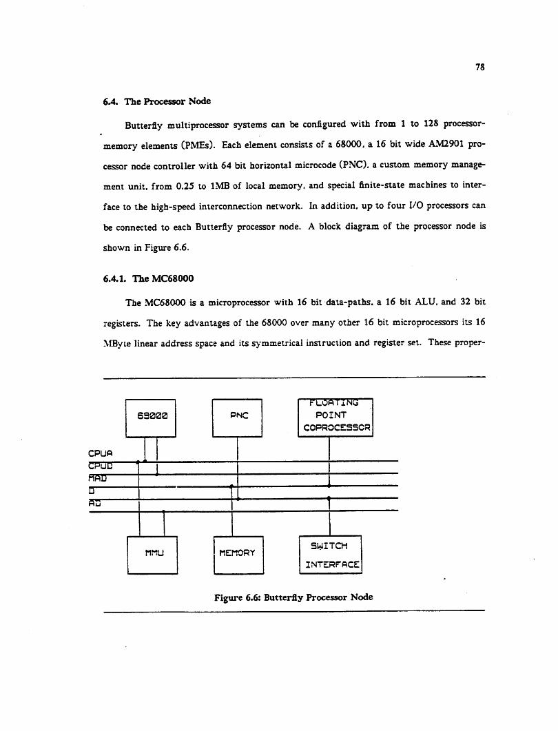
78
6 A The Processor Node
Butterfly multiprocessor systems can be configured with from 1 to 128 processor-
memory elements (PMEs). Each element consists of a 68000. a 16 bit wide AM2901 pro
cessor node controller with 64 bit horizonul microcode (PNC), a custom memory manage
ment unit, from 0.25 to 1MB of local memory, and special finite-state machines to inter
face to the high-speed interconnection network. In addition, up to four I/O processors can
be connected to each Butterfly processor node. A block diagram of the processor node is
shown in Figure 6.6.
6.4.1. The MC68000
The MC68000 is a microprocessor with 16 bit data-paths, a 16 bit ALU. and 32 bit
registers. The key advantages of the 68000 over many other 16 bit microprocessors its 16
MByte linear address space and its symmetrical instruction and register set. These proper-
ssaaa PNC
FLOATING
POINT
COPROCESSOR
CPUfl
CPuD
HAD
D
Hu
mmu MEMORYSWITCH
INTERFACE
Figure 6.6: Butterfly Processor Node

79
ties allow the 68000 to run large programs efficiently. More information on the 68000 is
available in [79] and related documents. In the Butterfly, the 68000 is extended by func
tions which execute in the AM2901-based processor node controller. All user code exe
cutes on the 68000. but system primitives are implemented in microcode on the PNC. All
memory references by the 68000 go through the MMU and are translated to network wide
physical addresses.
6.4.2. The Processor Node Controller
The processor node controller, or PNC. is a microcoded machine with 16 bit dau-path
and 64 bit wide microcode. A block diagram of the PNC is given in Figure 6.7. The PNC
and MMU are responsible for translation of all memory addresses which emanate from the
20 BRANCH CONOITIONS
MICROPROGRAM
SEQUENCER
C
33 FUNCTION REQUESTCONTROL LINES ]
MICRO INTERRUPTSERVICE ROUTINE
AOOHE5S0ENEHATOR
10 |
<KiW -BITREAOONLYCONTROL
STOM5MtYOHV
rW\
19
it
'2!
c CONTROL STORE AOORCSS BUS
T*
CONTROL LINES TO OTHERPROCESSOR NOOE RESOURCES
1f.8lT 2901ARITHMETIC/
LOGIC UNIT
rDATA BUS
Figure 6.7: The Processor Node Controller
80
MC68000. All references to normal memory are passed through the memory management
unit and converted from a system wide virtual address to a physical address on one of the
processor nodes.
6.4.3. The Switch Interface
The interconnection network in the Butterfly Multiprocessor is a base-4 Omega net
work, with 4-bit wide communications paths between the switches. Because the Omega is
a blocking network, the processor-node-controllers execute a protocol where an attempt is
made to send a message through the switch, and if the attempt fails, the request is re-tried
after a pseudo-random amount of time. The interface to the switch is provided by two
special-purpose finite-sute-machines. Diagram of the transmitter and receiver switch
interfaces are shown in Figure 6.8 and Figure6.9 respectively.
6.5. The Butterfly Operating System
The Chrysalis operating system [74] is a collection of subroutines which allow user
processes to manage local and shared resources. The features of this operating system
include object management, primitives for constructing message systems, and support for
atomic operations, all of which are described in more detail below.
6.5.1. Object Management
All resources in the Butterfly are considered to beobjects. These objects are identified
by a 32 bit quantity called an object handle. The object handle specifies the processor the
object resides on and the offset of the control block which identifies it in the F8 segment
on that processor. The format of an object handle is shown in Figure 6.10. The simplest
kind of object is a segment of memory. Memory objects are special in that they can be
placed directly into the address space of a process in such a way that no translation need
be done before the object is used. This process of entering a memory object into a process's
address space is called mapping in that object. When a memory object is mapped in. the

PNC Control S*Mb
UL J-
n
Tnmmttur Control IProarammaDta lo«>«|
TranwnittarContra*
Stera a
Syndtranowtftacjour _n
Ok
-t
To PNC tMiorainurruot
Sarvioa RontwaAddran Ganarttor
•LA
_»
Patn EnaotaRatj
ED
Om But
from PNC -Mtcronoda
TTA Port A
Com
18 a IB-bit DualPOrt ff AM
BCom PortB
Oata/ChaauumProoiarnrnaDiaLot* Amy fT
to/from BuRtrtlySwitcn Input *ort
Figure 6.8: Butterfly Switch Transmitter Interface
81

.'3
PNC Control Signals
lvReceiver Control
Programmable LogicArrayry
ReceiverControl
Store (7
.'»«
Synchronous ^ ClkRegister
Jl
.'*
To PNC MierointerruptService Routine
Address GeneratorPLA
HeaderChecksum
Register
to/from ButterflySwitch Output Port
>«.-«
ChecksumPLA f
T
ChecksumRegister
IT
Clk
from PNC -Micronode
Data Bus
Switch DataInput <
Register fT
Clk
Data Delay . ClkRegister p
A Port ACont
16x16x 16-bit DualPort RAM
BCont Port B |T
Figure 6.9: Butterfly Switch Receiver Interface
31 24
PROCESSORnode:
♦4JTBER
16
ECLENCE
NUMBER
OH-SCT IN
segment rs
Figure 6.10: Object Handle Format
e
82
system creates a new SAR to describe the segment, and then enters the new SAR in the
process's array of SARs. From that point on. no matter where the segment is in the global
address space of the machine, it can be referenced transparently just by the 68000
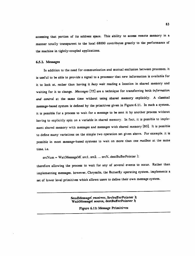
83
accessing that portion of its address space. This ability to access remote memory in a
manner totally transparent to the local 68000 contributes greatly to the performance of
the machine in tightly-coupled applications.
6.5.2. Messages
In addition to the need for communication and mutual exclusion between processes, it
is useful to be able to provide a signal to a processor that new information is available for
it to look at. rather than having it busy wait reading a location in shared memory and
waiting for it to change. Messages [75] are a technique for transferring both information
and control at the same time without using shared memory explicitly. A classical
message-based system is defined by the primitives given in Figure 6.11. In such a system,
it is possible for a process to wait for a message to be sent it by another process without
having to explicitly spin on a variable in shared memory. In fact, it is possible to imple
ment shared memory with messages and messages with shared memory [80]. It is possible
to define many variations on the simple two operation set given above. For example, it is
possible in most message-based systems to wait on more than one mailbox at the same
time. i.e.
srcNum = WaitMessageM( srcl. src2.... srcN. destBufferPointer ):
therefore allowing the process to wait for any of several events to occur. Rather than
implementing messages, however. Chrysalis, the Butterfly operating system, implements a
set of lower level primitives which allows users to define their own message system.
SendMessage( receiver, SrcbufferPointer );WaitMessage( source, destBufferPointer );
Figure 6.11: Message Primitives
84
6.5.3. Events
An event is a synchronization mechanism which can be used to implement message-
based systems. This technique has been used in the OS/360 and the MOS operating system
[74] and has been proposed for a variety of others. Events are created by a process (which
is then called a server process) and given to other processes (often called client processes).
When a client process wishes some service from a server process, it posts the event with
some information that the server may use: for example, it may post the object handle of a
buffer containing information that the client wishes to send to theserver. Aserver process
may have any number ofevents outstanding which have not been posted, and may or may
not decide to service an event once it is posted. However, in most cases, it is not permissi
ble for an event to be posted more than once without being reset, even though several
clients may have the ability to post it. Events are objects, as are all shared resources in
Chrysalis. Each has a global name, called an event-handle, which is valid across all pro
cessors.
6.5.4. Dual Queues
A dual-queue is a synchronization mechanism for event based systems. A dual-queue
may at any time hold data orevent-handles, but not both. When a server process tries to
dequeue a data-item from a dual-queue, it also passes an event-handle as one of the argu
ments in the call to dequeue. If there are data-items in the queue, the dequeue proceeds
normally. If. however, the queue is empty, or there are event handles in the queue, the
event handle passed to dequeue isentered into the dual-queue. When a client process tries
to enqueue a data-item into a dual-queue, the enqueue function checks to see if there are
event-handles or data-items in the queue. If there are data-items, the enqueue proceeds
normally. If however, there are one or more event-handles, then the first event handle is
removed from the queue, and the event is posted with the dau that was to be enqueued.
The result is that it is possible for servers to have request queues which are known by
85
client processes and for servers to wait until a data-item is entered into the queue by a
client process and then wake-up and process the data-item. Because events and dual-
queue are implemented in microcode on the processor node controllers, these mechanisms
are extremely fast. In fact, enqueue and dequeue operations execute in 10-15 fxs on the
current Butterfly.
6.5.5. Special addresses
Segment F8 of the virtual address space of each process is mapped into physical
memory starting at location zero. Because segment F8 is always mapped in starting at
zero, virtual addresses in that range can be converted to physical addresses by simply
deleting the upper bits of the address, and it is not necessary to go through the MMU.
Thus, addresses in segment F8 can be referenced in one less cycle than addresses in other
segments. Atomic operation, which allow a constant to be added to or subtracted from a
shared location without locking and without the mutual-exclusion problems described
above, are provided by referencing special locations.
6.6. The Floating-Point accelerator
The Berkeley Butterfly floating-point accelerator was designed and implemented by
Doreen Y. Cheng [81] and the Author. Although the MC68000 has integer performance
approaching that of a super-minicomputer, its floating-point performance is very poor
because it lacks floating-point support and such operations must be implemented in
software rather than a combination of microcode and hardware. [8l] contains information
on the performance of a variety of software floating-point packages which are available for
the MC68000. In general, there is a tradeoff between speed and accuracy in these packages.
For example, the software package which implements IEEE standard floating point arith
metic is an average of 2.5 limes slower than the Motorola FFP fast floating-point package.
However, the accuracy and quality of rounding of the IEEE package is significantly better
86
than the faster but less accurate FPP routines. In either case, software floating point
operations take considerable time. For example, the IEEE routines take approximately
100/xs to perform a floating-point add or multiply. This is approximately 100 times
slower than the integer performance of the MC68000. The result at the system level is
that if floating-point operations account for 10% of all operations, the system performance
on floating-point intensive applications is reduced to only 10% of its performance on pure
integer problems. To eliminate this bottleneck, the Butterfly floating-point accelerator was
designed to implement efficiently both scalar arithmetic functions as well as the more
complex operations specific to circuit simulation, such as MOS model evaluation, submatrix
solution, convergence checking, and automatic time-step selection.
The lack of a co-processor interface on the 68000 makes it difficult to pass operands
between it and the FPP. For example, the simplest method to pass data between them
would be to write the operands into two special locations in memory and read the result
from a third one. The problem with this approach is that the data transfers take a sub
stantial amount of time. For example, on the MC68000 a good lower bound on the execu
tion time of an instruction can be estimated by assuming that operations are always bus-
limited. A move instruction must specify both the source and the destination address.
Assume that the operands are in registers and that the result is to be returned to a register.
An instruction to move the first operand to the first magic location would consist of three
16 bit words: one for the basic instruction and two for the 32 bit destination address.
Such an instruction would take 5 basic operation times to execute. Three for the instruc
tion and two to write the data. The same amount of time would be required to move the
second operand, and the same for reading the result, for a total of 15 basic instruction
times. In the MC68000 every 16 bit operation requires four clock cycles, so that with an
8MHZ clock and no wait states, the time required for such a basic operation is 500ns.
Thus the minimum amount of time necessary to store the operands and return the result
would be 7.5/us. If the operands and result were in main memory, rather than registers.

87
the total time required would increase to 13.5fis. Any time required for the operation on
the board must be added to these times. The calling sequences defined below are designed
to decrease the time necessary to perform these operations. However, even as they are.
they still compare quite favorably with the time necessary for current co-processor chips
on processors which support such interfaces. For example, the NS16081 requires 7.4/xs for
a floating-point addition when both operands are in the floating-point unit's registers and
the result is returned to a FPA register. The Intel 80287. co-processor for the iAPX-286
requires 14 fis for the same operation.
CHAPTER 7
THE MSPLICE Program
7.1. Introduction
The MSPLICE program implements the DITA algorithm described above. MSPLICE uses a
single central counter, multiple schedulers, and distributed model-evaluation and conver
gence checking. The MSPLICE program has been designed to be compatible with the input
and output formats of the SPLICE program. Thus SPLICE input and output processors,
such as BLT [82] and SPLOT [14] may be used in conjunction with MSPLICE. In addition.
MSPLICE can also accept files in sim [83] format. A diagram of the MSPLICE program and
its input and output processors is shown in Figure 7.1.
7.2. The MSPLICE Program
The overall program flow of the MSPLICE program is shown in Figure 7.2 [16]: Here.
T represents the current value of simulated time in units of Minimum Resolvable Time
(MRT). and the forall construct means execute the block on all members of the set in any
order and. therefore, they may be executed concurrently.
73. Scheduling Algorithms
The major loop of the program is to take the next event off of the time-queue, process
the event, and schedule zero or more new events. The actions of taking an event off of the
event-queue, and of entering new events onto it. are performed by the scheduler routines.
Thus, it is desirable that these routines be as efficient as possible. The simplest type of
scheduler is a linked list of events sorted by the virtual time of the event's occurrence.
For efficiency reasons, time is usually represented as an integer number of basic units of
88

89
Figure 7.1 - The MSPLICE System
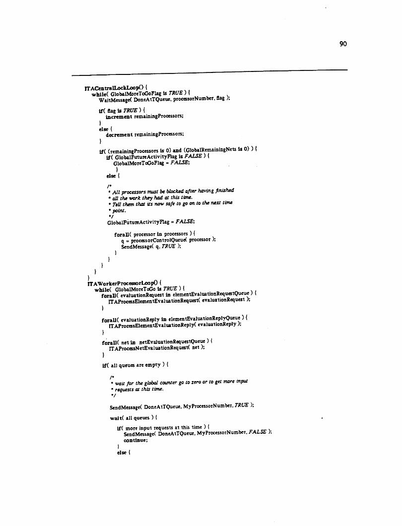
ITACcntralLockLoopO {while( GlobalMoreToGoFLag is TRUE) {
WaitMessageC DoneAtTQueue, processorNumber, flag ;;
if( flag is TRUE ) {increment remainingProcessors;
>else{
decrement remainingProcessors;
>
if( (remainingProcessoTS is0) and (GlobalRemainingNets is0) ) {if( GlobalFutureActivityFlag is FALSE) {
GlobalMoTeToGoFlag = FALSE;)
else{
/•• All processors must be blocked after having finished• all the vork they had at this time.• Tell them that us nowsafe togo onto thenext time• point.•/
GlobalFutureActivityFlag = FALSE;
forall( processor in processors ) {q =processorControlQueue( processor );SendMessage( q. TRUE );
)
}
ITAWorkerProcessorLoopO {while( GlobalMoreToGo is TRUE ) {
forall( evaluationRequest in elementEvaluationRequestQueue ; \ITAProcessElementEvaluationRequest( evaluationRequest );
}
foralK evaluationReply in elementEvaluationReplyQueue ) {ITAProcessElementEvaluattonReply( evaluationReply ;:
}
foralK net in netEvaluationRequestQueue ) {ITAPTOcessNetEvaluationRequesti net );
}
if ( all queues areempty ) {
/•• vaitfor the global counter go to zero ortoget more mput* requests at this time.V
SendMessage( DoneAtTQueue. MyProcessorNumber, TRUE );
wait( all queues ) {
if( more input requests at this time ) {SendMessage( DoneAtTQueue, MyProcessorNumber. FALSE );continue;
Ielse{
90

}
T = T + 1;swap evaluation queues for T and T+l;schedule any input sources at T-rl;
}
ITAProcessElementEvaluationRequest( evaluationRequest ) {net = evaluationRequest- >net;element » evaluationRequest- >element;Norton = ITACompanionModelC net,element);q » elementEvaluationReplyQueue( homejjrocessoK net) )reply- >net = net;reply- >Norton = Norton;sendMessage( q, reply );
ITAPTocessE3exnentEvaluatlonReply( evaluationReply) {net « evaluationReply- >net;faninNorton = evaluationReply- >Norton;net- >Norton » net- Norton + faninNorton;net->remainingFanins » net->remainingFanins -1;
if( net- >remainingFanins is 0 ) {ITACheckConvergence( net);
}
ITAPTOcessNetEvaluationRequest( net) {foralK fanin_element in net) {
q =elementjvaluationjaueue(home_processor(fanin_cleinent));request- >net » net;request- >element = fanin_element;sendMessage( q, request );
>}
/•• Check convergence, schedule selfand fanouts. and keep GlobalRemainingNets• (the global count ofthe number ofnets under evaluation) consistent.
ITACheckConvergence( net ) {if( net has converged at this time ) {
if( net has not previously converged at this time point ) {if( change from the previous time point is significant) {
schedule the net at T-l;if( T+l queue has just become non-empty ) {
GlobalFutureActivityFlag = TRUE;)schedule the net's fanouts at this time point;increment GlobalRemainingNets by Nfanouts-1;
else {re-schedule the net at this time;
>decrement GlobalRemainingNets;
Figure 7.2 - MSPLICE Program Flow
91

92
time. The unit, called minimum resolvable time or MRT. represents the smallest time inter
val over which a meaningful event can occur in the circuit being simulated. If the events
to be scheduled were uniformly distributed in time, then the time complexity of adding a
new event to the queue would be -^ for a list of N events. However, the distribution of
event-times is usually quite skewed, with many events scheduled at the next step in simu
lated time, and far fewer events scheduled in the distant future. There are several ways
to take advantage of this fact. The SPLICE1 program [14] optimizes access to events which
occur within 200 units of the current time by using a combination of two arrays of
pointers and a linked list. The disadvantage of this approach is that it requires that when
the event-list for the current time is finished slots in the pointer arrays must be examined
sequentially until a non-empty one is found. However, since in practice most events are
scheduled at either the current time or one unit of MRT in the future, [6] empty slots are
rarely encountered. The MSPLICE program currently uses a single global time-step. Thus,
when an electrical node which is not directly driven by an input or a timing source
(clock) is scheduled, it can only be scheduled at the current time or one unit of MRT in
the future. To take advantage of this. MSPLICE uses a scheduler with two queues, one for
the current time and one for the time one unit of MRT in the future. Primary inputs
treated as a special case, and are scheduled at every point in time during the simulation
interval. The MSPLICE program uses the Gauss-Seidel-Newton algorithm described ear
lier, but can also be run using a less constrained variation of the algorithm known as
weakly chaotic relaxation [84]. In this case, a PME can continue to solve a node for itera
tions k +1X +2. • • • k +Fm. where Fm is the maximum number of iterations a node can
move ahead before it must wait for updates of the values of its fanin node voltages. For
Gauss-Seidel-Newton. Fm = 1.
93
7.4. Primary Inputs
The data-structure for a primary input consists of an entry for the current delta-v. a
state counter, a remaining-time counter and a state-transition table. Every time the pri
mary input model is called, the remaining-time counter is decremented. When the
remaining-time counter reaches zero, the state of the timing-source is changed to next
state, the current delta-v value is set to the delta-v value for the new state, and the
remaining-time counter is set to the duration of the new state. The advantage of this
approach is that it allows events to be entered and removed from the queue extremely
quickly. The disadvantage is that it requires that primary inputs be processed even when
they are latent. However, because most circuits have many more internal nodes than pri
mary inputs, the advantages strongly outweigh the disadvantages. For example, in a
medium-size industrial circuit, a digital filter circuit having 704 transistors and 345 nodes,
there are only four clocks and external inputs. The time spent processing timing sources
and external inputs for this circuit was less than 0.2% of the total simulation time. As
circuits become larger, the ratio of the number of internal to external nodes should become
even larger. However, no matter how fast a scheduler is. it is always possible to add
enough evaluation units so that it becomes the limiting factor in simulator performance.
To eliminate this problem, the MSPLICE program uses a separate scheduler on each proces
sor. However, as mentioned earlier, these schedulers must be kept in loose synchroniza
tion. To maintain numerical consistency in the DITA approach, it is necessary to insure
that all nodes that can affect a given node at timeT have converged at T before processing
the node for T+l. One way to do this is to keep track of the number of unconverged
nodes (equations) in the system and prevent any nodes from being processed at T+l until
all have converged at T.

94
7.5. The convergence counter
MSPLICE implements the most straight forward form of this algorithm, by main
taining a central count of the number of unconverged nodes (equations) in the system.
The counter is a resource shared by all processes. However, because it need only be incre
mented or decremented and checked against zero, access can be made to it quite quickly.
The convergence counter is kept in a piece of shared memory, and can be incremented
and decremented by messages to a process which is responsible for maintaining it. The
advantage of the shared memory approach is speed. However, it is essential that either the
increment and decrement are available as atomic operations or that the counter be locked
and unlocked whenever it is necessary to access it.
In the Butterfly version of MSPLICE. it is possible to use either approach. Normally,
there is a watcher process which is responsible for maintaining the convergence counter.
Whenever a simulation process wishes to increment or decrement the counter, it sends a
message to the watcher process by enqueueing the value is wishes to add to the counter
onto a dual-queue which contains an event handle owned by the watcher process. This
causes the watcher process to wake up and modify the convergence counter accordingly.
Note that while the counter is being modified by the watcher process, any requests which
come in will simply be queued up waiting for the watcher to dequeue them. The
MSPLICE program can also be configured to run without a watcher process. In that ver
sion, the code from the watcher process is run whenever a process increments or decre
ments the convergence counter. Normally, this would require that the convergence
counter be locked before being accessed. However, the Butterfly multiprocessor allows this
process to be avoided by providing atomic increment and decrement operations.
7.6. Model evaluation
In the MSPLICE program, model evaluation is distributed on a per-node basis.
Whenever a node is solved, the processor solving it is responsible for evaluating the model

95
for each of its fanin elements. This approach results in high performance and high
efficiency for solving large circuits on large numbers of processors. For very small circuits,
it may be more desirable to have each transistor, rather than each net. be processed in
parallel.
7.7. Program Performance
The performance of MSPLICE on the digital-filter circuit is shown in Table 7.1. In
all cases, as the number of processors were increased the program execution time decreased.
Note that for 9 processors, the speedup and efficiency of MSPLICE on the Butterfly was
90% of the theoretical maximum, given by the unit delay model.
Currently, as a result of the low floating-point performance of the prototype
machine, model-evaluation and convergence checking are the rate-determining steps of the
Butterfly MSPLICE implementation. However, a new floating-point accelerator/model-
evaluation-unit is under construction which should considerably improve the ability of
the machine to perform these tasks [81]. As mentioned above, queue management is
implemented in microcode and is quite fast.
Processors Speedup Efficiency
1 1.00 1.00
2 1.83 0.92
3 2.28 0.76
4 3.40 0.85
5 4.09 0.82
6 4.55 0.76
7 5.33 0.76
8 5.98 0.75
9 6.77 0.75
10 7.04 0.70
Table 7.1 - Digital Filter Speedup
96
7.8. Communications Requirements and Scaling
It is possible to calculate the communications requirements of the algorithm and theload that would be seen by the network as the performance of the individual nodes is
increased. If distributed counter management and random assignment of sub-circuits to
processor nodes are used, it can be assumed that aprocessor will have an equal probabilityof accessing any other processor's memory, and auniform reference model can be used forICN load. Given that several fanin elements must be evaluated to determine the value of a
node, and that convergence checking can performed locally, an upper bound on the traffic
which can be generated is given by assuming that all nodes are performing model evaluation at all times. If an MOS model evaluation evaluation could be performed every lOus .
then every port of the network would see a reference every 8.33 fis for NMOS circuitsand 6.7 fis for CMOS. Thus, a 16 processor system would require a network capable ofservicing a request every 416 to 520 ns. which is well within the limits of current fastbusses. However, for a 256 processor system, a request would be seen every 26.2 to 32.5ns. It is currently difficult to make busses which run at such speeds and are aphysicallylarge enough for a 256 processor system. One alternative network is the single stageperfect-shuffle [85] If such anetwork was built to have a100 ns cycle, it would see aloadof 1.2 - 1.5 %at each port. At such low loads, such networks experience very few colli
sions, and their delay can be expected to be in the range of log(N). where Nis the number
of ports in the network, so aremote reference on such asystem could be expected to take=s 800/15. less than 10% of the model evaluation time.
If the basic steps of scheduling, model-evaluation, and convergence checking can be
performed at a lOfis rate, and 50% efficiency can be achieved for a25.000 node circuit(=70.000 MOSFETS). then through acombination of algorithms and architecture a totalsystem performance equivalent to aconventional computer running SPICE2 at almost 4GFLOPS can be achieved. The result is that the analysis of a 70.000 MOSFET circuit on

97
this machine would take about the same time as the analysis of a 20 transistor circuit on a
VAX-11/780.

CHAPTER 8
CONCLUSIONS
An approach to provide very high speed circuit simulation, based on relaxation techniques,
special-purpose hardware, and effective use of multiprocessors has been described. Investi
gations of models of parallel computation, multiprocessor computer architecture architec
ture and interconnection networks has led to a proposed architecture for a circuit simula
tion machine. Circuit simulation has been implemented on both small grain (data-flow)
and large grain (process based) multiprocessor systems. The data-flow model of computa
tion and functional programming languages have been explored in the context of circuit
simulation. The program ITA/DF. a test implementation of the ITA circuit simulation
algorithm has been developed in SISAL (Streams and Iteration in a Single Assignment
Language), and tested on an experimental data-flow computer, the Manchester dau-flow
machine, and high speedup was observed for up to 13 processors when simulating a small
circuit. Based on these results, a new distributed circuit simulation algorithm - Distri
buted Iterated Timing Analysis (DITA). has been developed. DITA which allows subcir
cuits to be solved by independent processors while providing a consistent global solution
to the circuit as a whole. The DITA algorithm has been implemented in the program
MSPLICE and executed on an experimental process-based multiprocessor, the Bolt Beranek
and Neumann (BBN) Butterfly system. A floating-point co-processor for the Butterfly sys
tem has been developed, and an architecture for a special processor for evaluation of MOS
models has been proposed. Initial results are promising, with greater than 70% efficiency
on a 10 processor system when simulating a large industrial circuit.
There are many possible directions for future research. They fall into several
categories:
98
99
1. Improvements to the Algorithms in MSPLICE.2. Special Purpose hardware.3. Higher Multiprocessor Efficiency.
First, there are many areas in which the MSPLICE program can be enhanced to increase
performance and robustness. Automatic partitioning, either static or dynamic, of the cir
cuit into subcircuits should be added to improve the program's performance when simulat
ing circuits with tightly coupled nodes. Variable time-step control should be added to
MSPLICE to free the user from time-step selection and increase robustness. The program
should be made more interactive to allow results to be viewed as the simulation progresses
and to allow the user to change the circuit parameters and topology interactively. Second,
experience with the Butterfly floating-point accelerator will lead to a better understanding
of what is needed in special-purpose hardware for circuit simulation. Finally, changes in
the algorithms to eliminate the need for all nodes to converge at time T before any go on
to time 7 +1 will allow greater multiprocessor efficiency.
REFERENCES
1. Newton. A. R. and A. L. Sangiovanni-Vincentelli. "Relaxation-Based Electrical
Simulation". IEEE Transactions on Computer Aided Design CADS. 4 (October 1984).
308-329. IEEE.
2. Kleckner. J. E.. R. A. Saleh and A. R. Newton. "Electrical Consistancy in Schematic
Simulation". Proceedings of the ICCC. New York. Sept 1982. 30-33.
3. Case. G.. "The SALOGS Digital Logic Simulator". Proc. 1978 IEEE International
Symposium on Circuits and Systems, New York. May 1978. 5-10.
4. Jenkins. F.. ILOGS: User's Manual. Simutec Corporation. 1982.
5. Bryant. R. E.. "An Algorithm for MOS Logic Simulation". LAMBDA. 4th Quarter
1980. 46-53.
6. Newton. A. R.. "The simulation of large scale integrated circuits". IEEE Trans, on
Circuits and Systems CAS-26 (September 1979). 741-749..
7. Burns. J. L.. "Empirical Mosfet Models for Circuit Simulation". Electronics Research
Lab. Memorandum, Berkeley. Ca.. May 1984.
8. Cohen. E.. "Performance Limits of Integrated Circuit Simulation on a Dedicated
Minicomputer". UCB/Electronics Research Lab. Memo M81. 29 (May 1981).
University of California. Berkeley.
9. Kron, G.. Diakoptics - Piecewise Solution of Large-Scale Systems. MacDonald. London.
1963.
10. Yang. P.. I. N. Hajj and T. N. Trick. "SLATE: A Circuit Simulation Program with
Latency Exploitation and Node Tearing". Proc. IEEE Int. Conf. on Circ. and Comp.
October 1980.
101
102
11. "The CRAY X-MP Series of Computers". Pub No. MP-0001. Cray Research. Mendota
Heights. MN. 1982.
12. Charlesworth. A. E.. "An Approach to Scientific Array Processing: The Design of the
AP-120B/FPS-164 Family". Computer Magazine Vol 14. 9 (Sept. 1981). IEEE
13. Calahan. D. A. and W. G. Ames. "Vector Processors: Models and Applications". IEEE
Trans, on Circ. andSyst. Vol. CAS-26 (September 1979).
14. Saleh. R. A.. Iterated Timing Analysis and SPLICE1. Electronics Research Laboratory.
University of California, Berkeley.
15. Kleckner. J. E.. "Advanced Mixed-Mode Simulation Techniques". PhD. Dissertation,
University of California, Berkeley. Berkeley. Ca. 1984.
16. Deutsch. J. T. and A. R. Newton. "A Multiprocessor Implemenution of Accurate
Electrical Circuit Simulation". Proceedings, 19th ACM/IEEE Design Automation
Conference, Las Vegas. Nv.. 1984.
17. Dennis. J. B.. "Data-Flow Supercomputers". IEEE Computer 13. 11 (Nov. 1980). 48-
56.
18. Rettberg. R. and C. Wyman. "Development of a Voice Funnel System: Design
Report". BBN Report M098, August. 1979.
19. Schriber. T. J.. A GPSS Primer. John Wyley. New York. 1976.
20. Hill. D. D.. "Language and Environment for Multi-Level Simulation". Ph.D.
Dissertation, Stanford University. Stanford, CA. 1980.
21. Deutsch. J. T. and A. R. Newton, "Data-flow based behavioral-level simulation and
synthesis". IEEE ICCAD Conference. Sept 1983.
22. Newton. A. R. and D. 0. Pederson. "Analysis Time. Accuracy and Memory
Requirement Tradeoffs inSPICE2". Proceedings, Asilomar Conference. 1978.
103
23. Pfister. G. F., "The Yorktown Simulation Engine: Introduction". Proceedings, 19th
ACM/IEEE Design Automation Conference. June 1982. 51-54.
24. Howard. J. K.. L. Malm and L. M. Warren. "Introduction to the IBM Los Gatos Logic
Simulation Machine". Proceedings IEEE International Conference on Computer Design,
Oct. 1983. 580-583.
25. Dunn. L. N.. "IBM's Engineering Design System Support for VLSI Design and
Verification". IEEE Design and Test of Computers 1. 1 (Feb. 1984). 30-40. IEEE.
26. Denneau. M. M.. "The Yorktown Simulation Engine". Proceedings, 19th ACM/IEEE
Design Automation Conference. June 1982. 55-59.
27. Kronstadt. E. and G. Pfister. "Software Support for the Yorktown Simulation
Engine". Proceedings, 19th ACM/IEEE Design Automation Conference. . 60-64.
28. Hofmann. M.. "Automated Synthesis of Random Sequential Digital Logic in CMOS
Technology". Ph.D. Dissertation, University of California, Berkeley. Berkeley, Ca..
May 1985.
29. "CAE Sution's Simulators Tackle 1 Million Gates". Electronic Design. Nov. 1984.
30. Blank. T.. "A Survey of Hardware Accelerators Used in Computer-Aided Design".
IEEE Design and Test of Computers 7.21-39. IEEE
31. Gurd. J. R.. C. C. Kirkham and I. Watson. "The Manchester Prototype Dauflow
Computer". Comm. of the ACM 28.1 (Jan 1985). 34-52. ACM.
32. Nagel. L. W.. "SPICE2 A Computer Program To Simulate Integrated Circuits'.
Electronics Research Lab. Memo UCB/Electronics Research Lab. M75/20 (1975).
University of California. Berkeley.
33. "Advanced Sutistical Analysis Program (ASTAP). Program Reference Manual". IBM
Corp.. White Plains. NY. .

104
34. Jenkins. F.. ASPEC Users Manual.
35. Hofmann. M. and U. Lauther. "HEX: An Instruction-Driven Approach to Feature
Extraction". Proceedings, 20th ACM/IEEE Design Automation Conference. 1983.
36. "CDC Cyber 200 Model 203 Computer System Hardware Reference Manual". Pub.
No. 60256010. Control Dau Corporation. St. Paul. MN„ May 1980.
37. Vladimirescu. A. and D. 0. Pederson. "Performance Limits of the CLASSIE Circuit
Simulation Program". Proceedings, International Symposium on Circuits and Systems,
Rome. May 1982.
38. Chua. L. O. and P. M. Lin. Computer-Aided Analysis of Electronic Circuits: Algorithms
and Computational Techniques. Prentice-Hall. Englewood Cliffs. N.J.. 1975.
39. Duff. I. S.. "A Survey of Sparse-Matrix Research". Proceedings of the IEEE. Apr.
1977.
40. Sakallah. K. A.. "Mixed Simulaton of Electronic Integrated Circuits". Report DRC-
02-07-8l.EE Department, Carnegie-Mellon University. Nov. 1981.
41. Ko. F. W. and A. L. Sangiovanni-Vincentelli, Blossom: An Algorithm and
Architecture for the Solution of Large Scale Linear Systems.
42. Kieckhafer. R. M.. "Development of A Processor Array Architecture for Application
to Circuit Simulation". PhX>. Dissertation, Cornell University. 1983.
43. Chawla. B. R.. H. K. Gummel and P. Kozak. "MOTIS-an MOS timing simulator".
IEEE Trans, on CAS vol. CAS-22 (Dec. 1975). 901-909.
44. Larasmee. E.. A. Ruheli and A. L. S. Vincentelli. "The Waveform Relaxation Method
for the Time-Domain Analysis of Large Scale Integrated Circuits". IEEE Tran. on
CAD of Int. Circ. and Sys CAD 1, 3 (Aug 82). 131-145.
45. White. J. and A. L. Sangiovanni-Vincentelli.. "Relax2.1: A Waveform Relaxation
Based Circuit Simulation Program". Proceedings, IEEE Custom Integrated Circuits

105
Conference. Rochester NY. May 1984.
46. Newton. A. R.. "Pidgin 'C: The only way to fly". Electronics Research Lab.
Memorandum, University of California, Berkeley. Berkeley. Ca.,.
47. Saleh. R. and A. R. Newton. "Iterated timing analysis and SPLICEl". Proc. IEEE
1CCAD Conference. Santa Clara. Ca.. Sept. 1983.
48. Yu. W. H.. "LU Decomposition on a Multiprocessing System with Communications
Delay". Ph.D. Dissertation, EECS Department, University of California, Berkeley.
Berkeley. Ca.. 1983.
49. Kuck. D. J.. The Structure of Computers and Computations, John Wiley and Sons.
1976.
50. Barnes, G. H.. R. M. Brown. M. Kato. D. J. Kuck. D. L. Slotnick and R. A. Stokes.
"The ILLIAC IV Computer". IEEE Transactions on Computers C-17. 8 (Aug. 1968).
746-757. IEEE.
51. Ramamoorthy, C. V.. Private communications.
52. Flanders. P. M.. D. J. Hunt and S. F. Reddaway. High Speed Computer and Algorithm
Organization. Academic Press. New York. 1977.
53. Batcher. K. E. "Bit-Serial Parallel Processing Systems". IEEE Transactions on
Computers C-31. 5 (May 1982). 377-384.
54. Rubin. F.. "The Lee Path Connection Algorithm". IEEE Transactions on Computers C-
23. 9 (Sept 1974). 907-914. IEEE.
55. Baker. C. M.. "Artwork Analysis Tools for VLSI Circuits". MS. Dissertation, M.I.T..
May 1980.
56. Hintz. R. G. and D. P. Tate. "Control Data STAR-100 Processor Design". Proceedings,
IEEE 1972 Computer SocietyConference. Sept. 1972. 1-4.
106
57. QSPICE users quide, Quantiutive Technology Corporation. Beverton Or..
58. Peterson. J. L.. Petri Net Theory and The Modeling of Systems. Prentice Hall.
Englewood Cliffs. N.J.. 1981.
59. Aho. A. V. and J. D. Ullman. Principles of Compiler Design. Addison-Wesley.
Reading. Ma.. 1979.
60. Padua. D. A.. D. J. Gajski and D. H. Lawrie. "High-Speed Multiprocessors and
Compilation Techniques". IEEE Transactions on Computers C-29. 9 (Sept. 1980).
763-776. IEEE
61. Arvind. K. P. Gostelow and W. Plouffe. A Data-Flow Programming Language and
Computing Machine, Department of Information and Computer Science. University of
California. Irvine. Irvine, Ca.. Feb. 1978.
62. Keller. R. M.. "A Loosely-Coupled ApplicativeMultiprocessing System". Proceedings,
AF1PS National Computer Conference. 1979.
63. Backus. J.. "Can Programming be Liberated from the Von-Neumann Style? A
Functional Style and its Algebra of Programs". Communications of the ACM 21. 8
(Aug. 1978). 613-641. ACM.
64. Ackerman. W. B. and J. B. Dennis. "VAL - A Value Oriented Algorithmic Language:
Preliminary Reference Manual". Tech. Rep.-218, 1979.
65. McGraw. J.. SISAL: Streams and Iteration in a Single Assignment Language.
Lawrence Livermore Laboratory. July 20. 1983.
66. Szygenda. S. A. and E. W. Thompson. "Digital Logic Simulation in a Time-Based.
Table-Driven Environment. Part 1. Design Verification". IEEE Computer. March
1975.24-36.
67. Feng.. T. Y.. "A Survey of Interconnection Networks". IEEE Computer. Dec. 1981.
12-27.

107
68. Lawrie. D. H.. "Access and Alignment of DaU in an Array Processor". IEEE Trans, on
Computers 24. 12 (December 1975). 1145-1155.
69. Broomell. G. and J. Heath. "Classification Categories and Historical Development of
Circuit Switching Topologies". Computing Surveys 15. 2 (June 1983). 95-133.
70. Goodman. J.. "A Study of Procesor-Cache Interaction". Proceedings, IEEE Compcon.
1983.
71. Seitz. C. L.. "The Cosmic Cube". Comm. of the ACM 28. 1 (Jan. 1985). 22-33. ACM.
72. Vladimirescu. A. and S. Liu. "The Simulation of MOS Integrated Circuits Using
SPICE2". Electronics Research Lab. Memo UCB/Electronics Research Lab. M80/7. Feb.
1980.
73. Kuck. D. J.. D. Lawrie. R. Cytron. A. Sameh and D. Gajski. "The Architecture and
Programming of the CEDAR System". Proceedings. 1983 LASL Workshop on Vector
and Parallel Processing. Los Alamos. NM.. 1983.
74. Rettberg. R.. F. Heart. B. Mann and J. Goodhue. The Chrysalis Operating System
Manual. Bolt. Beranek and Newman, June 1 1983.
75. Shaw. A. C. The Logical Design of Operating Systems. Prentice-Hall. Englewood
Cliffs. NJ. 1974.
76. Baker. H. G.. "Actor Systems for real-time compuution". M.I.T Tech Report
MIT/LCS/Tech. Rep.-197 .
77. Goldberg. A. and D. Robson. Smalltalk-80 The Language and its Implementation.
Addison Wesley. Reading Ma.. 1983.
78. Knuth. D. E. The Art of Computer Programming. Addison Wesley. New York. N.Y..
1973.
79. Suff. 68000 Users Manual, Motorola Corporation, Scottsdale Az..
108
80. Lauer. H. C. and R. M. Needham. "On the Duality of Operating System Structures".
Operating Systems: Theory and Practice, Amsterdam. 1979. 371-384.
81. Cheng. D. Y.. "A Floating-Point Co-Processor for the Butterfly Multiprocessor
System". Electronics Research Lab. Memo 84/55. Berkeley. Ca.. July 1984.
82. Crawford. J.. "A Unified Hardware Description Language for CAD Programs".
Electronics Research Lab. Memo. Aug. 1979.
83. Terman. C. J.. "RSIM - A Logic-Level Timing Simulator". Proceedings of the
International Conference on Computer Design. 1983. 437-440.
84. Chazan. D. and W. Miranker. "Chaotic Relaxation". Linear Algebra and Its
Applications 2 (1969), 199-222. American Elsevier.
85. Lang. T.. "Interconnections Between Processors and Memory Modules Using the
Shuffle Exchange Network". IEEE Trans. Computers. May 1976. 496-503.
110
APPENDIX A
Source Listing of Program ITA/DF
This appendix contains the source listing of Program ITA/DF. To obtain this
program contact Deborah Dunster at the following address:
EECS Industrial Liason Program
437 Cory Kail
University of California
Berkeley. CA 94720

124
APPENDIX B
Source Listing of Program MSPLICE
This appendix contains the source listing of Program MSPLICE. To obtain
this program contact Deborah Dunster at the following address:
EECS Industrial Liason Program
437 Cory Kail
University of California
Berkeley, CA 94720