..

The D* Algorithm for Real-Time Planning of Optimal Traverses

Anthony Stentz

CML-RI-TR-94-37

The Robotics Institute Carnegie Mellon University

Pittsburgh, Pennsylvania 15213 September 1994

CC 1994 Carnegie Mellon

This research was sponsored by ARPA, under contracts “Perception for Outdoor Navigation” (contract number DACA76-89-C-0014. monitored by the US Army TEC) and “Unmanned Ground Vehicle System” (contract number DAAE07-90-C-RO59, monitored by TACOM). Views and conclusions contained in this document are those of the author and should not be interpreted as representing ofiicial policies, either expressed or implied. of ARPA or the United States Government.

Table of Contents

1.0 Introduction 5 2.0 The Basic D* Algorithm 7

2.1 Intuition 7 2.2 Definitions 10 2.3 Algorithm Description 10

3.0 The Focussed D* Algorithm 14 3.1 Intuition 14 3.2 Definitions 16 3.3 Algorithm Extension 18

4.1 D* Comparisons 20 4.2 A Priori Map Information 23

4.0 Examples 20

5.0 Experimental Results 25

6.0 Conclusions 28

List of Figures

Figure 1 Figure 2 Figure 3 Figure 4 Figure 5 Figure 6 Figure 7 Figure 8 Figure 9 Figure 10 Figure 11 Figure 12 Figure 13

Invalidated States in the Graph Propagation of R A I S ~ and LOWER states Repir of Graph out to Robot is Complete Focussed RAISE State Propagation 14 Focussed LOWER States Reach Robot’s State 15 Computing a Lower Bound on A”) for Robot Motion Computing Bias Values for A”) Cluttered Environment 20 Basic D* Algorithm 21 Focussed D* Algorithm 22 Omniscient Optimal Traverse 23 Optimistic Optimal Traverse 24 Typical Environment for Comparison 25

7 8 9

16 17

Abstract

Finding the lowest-cost path through a graph of states is central to many problems, including route planning for a mobile robot. If arc costs change during the traverse, then the remainder of the path may need to br replannrd. Such is the case for a sensor-equipped mobile robot with incomplete or inaccurate information about its environment. As the robot acquires additional information via its sensors, it has the opportunity to revise its plan to reduce the total cust of the traverse. If the prior information is grossly incumplere or inaccurate, the robot may discover useful inforination in nearly every piece of sensor data. During the replanning process. the robot must either stop and wait for the new path to be computed or continue to move in the wrong direction; therefore: rapid replanning is essential. This paper describes a new algorithm, D*, capable of planning optimal traverses i n real-time through focussed state expansiun. D' repairs plans quickly by taking advantage of the fact that most arc cost corrections occur in the vicinity of the robot and the path needs only to be replanned out to the robot's current state. D* can be used not only for route planning but for any graph-based cost optimization problem for which arc costs change during the traverse of the solution path.

5

1.0 Introduction

The problem of path planning can be stated as finding a sequence of state transitions through a graph from some initial state to a goal state. or determining that no such sequence exists. The path is optimal if the sum of the transition costs. also callcd arc costs. is minimal across all possible sequences through the graph. If during the “traverse” of the path, one or more arc costs in the graph are discovered to be incorrect. the remaining portion of the path may need to be rcplanned to preserve optimality. A traverse is optimal if every transition in the traverse is part of an optimal path to the goal, assuming at the time of each transition, all known information about the arc costs is correct.

An important application for this problem, and the one that will serve as the central example throughout the paper. is the task of path planning for a mobile robot equipped with a sensor, operating in a changing. unknown or partially- known environment. The states in the graph are robot locations, and the arc values are the costs of moving between locations, based on some metric such as distance. time, energy expended. risk. etc. The robot begins with an initial estimate of arc costs comprising its “map”, but since the environment is only partially-known or changing. some of the arc costs are likely to be incorrect. As the robot acquires sensor data, it can update its map and replan the optimal path from its current state to the goal. It is important that the replanning is fast. since during this time the robot must either stop or continue to move along a suboptimal path.

The field of path planning has received considerable attention in the research literature (see Latombe [51 for a good survey), hut only recently has the problem of planning in unknown, partially-known, or dynamic environments been addressed. The algorithms can be divided into two classes. The first class consists of algorithms which are computationally fast and memory efficient, but which yield suboptimal traverses. Goto and Stentz [2] generate a ”global” path using the known information and then attempt to “locally” circumvent obstacles on the route detected by the sensors. If the route is completely obstructed. a new global path can he produced. Lumelsky [7] initially assumes the environment to be devoid of obstacles and then moves the robot directly toward the goal. If an obstacle obstructs the path. the robot moves around the perimeter until the point on the obstacle nearest the goal is found. The robot then proceeds to move directly toward the goal again. Pirzadeh 191 adopts a strategy whereby the robot wanders about the environment until i t discovers the goal. The robot repeatedly moves to the adjacent location with lowest cost and increments the cost of a location each time it visits it to penalize later traverses of the same space. Korf [4] uses initial map infomation to estimate the cost to the god for each state and efficiently updates it with backtracking costs as the robot moves through the environment. These algorithms are computationally fast because the “replanning” operations are mostly local decisions about which way to muve next. Little if any state information is retained during the traverse, so the algorithms are memory efficient. Because of the local scope of this replanning, however. completeness can be guaranteed but optimality cannot. This suboptimality can be extreme in some cases.

The second class of algorithms guarantees an optimal traverse but at greater computational and memory cost. One algorithm plans an initial path with A * [SI or the distance transform 131 using the prior map information. moves the robot along the path until either it reaches the goal or its sensors discover a discrepancy between the map and the environment, updates the map, and then replans a new path from the robot’s current state to the goal. Although this brute-force replanner is optimal. it can begrossly inefficient, panicularly in expansive environments where the goal is far away and little map information exists. Zelinsky 1151 increases efficiency by using a quad-tree [ l l ] to represent the free and obstacle space. thus reducing the number of states to search in the planning space. This approach is suboptimal or inefficient, however, if the state-to-state costs for moving through the environment range over a continuum.

Boult [i] maintains an optimal cost map from the goal to all states in the environment. assuming the environment is hounded (finite). When discrepancies are discovered between the map and the environment. the algorithm updates only the affected portion of the cost map. The map representation is limited to polygonal obstacles and free space. Trovato 141 and Ramalingam and Reps 1101 extend this approach to handle graphs with arc costs ranging over a continuutn. The limitation of this class of algorithms is that the entire affected portion of the map must he repaired before the robot can resume moving and subsequently make additional corrections to the map. Thus, the algorithms are inefficient when the robot is near the goal and the aftected portions of the map have long “shadows”.

6

This paper presents a new algorithm, D*, for generating optimal traverses in real-time through a graph with changing or updated arc costs. D* takes advantage of the fact that most arc cost corrections occur in the vicinity of the robot, and only the portion of the path from these corrections out to the robot’s current location needs to be replanned. D* mainvains a partial. optimal cost map limited to those locations likely to be of use to the robot. Likewise, repair of the cost map is generdlly partial. re-entrant, and limited only tu those states likely to yield a new. optimal path to the robot. D* establishes conditions fur deterniining when the repair can be halted, either because a new path is fbund or the old one is still optimal. Thus, D* is very cumputationally and memory efficient. and i t works i n unbounded environments as well.

The algorithm is formulated in terms of a repeated, optimal find-path problem within a directed graph. where the arcs are labelled with transition cost values that can range over a continuum. Arc cost corrections (e.& from a sensor) can be made at any time, and the known, measured. and estimated arc values comprise the map of the environment. The algorithm can be used for any planning representation, including visibility graphs [SI and grid cell structures. The paper begins with the basic form of the algorithm introduced by Stentz [ 131 and then describes new extensions to it that improve its computational and memory efficiency. Examples follow that illustrate the alEorithm in operation. Experimental results are presented that compare several variations of D* to the brute-force replanner. Finally. conclusions are drawn.

7

2.0 The Basic D* Algorithm

The aigorithnl is named D* because it resembles A* [8], except that it is dynamic in the sense that arc costs can change during the traverse of the solution path. Provided that the traverse is properly coupled to the replanning process, i t is guaranteed to be optimal. This section begins with the intuition behind the algorithm, defines the notation used. and presents D* as it was described in Stentz [13].

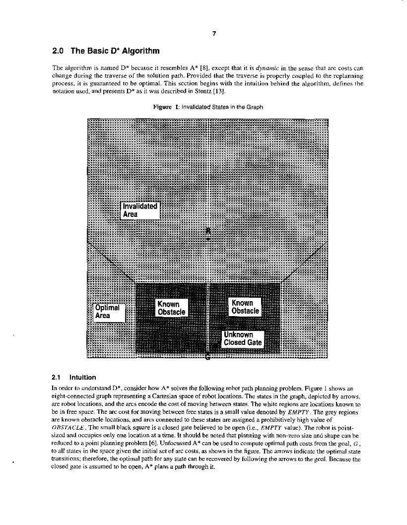
Figure 1: Invalidated States in the Graph

2.1 Intuition In order to understand D*. consider how A * solves the following robot path planning problem. Figure 1 shows an eight-connected graph representing a Cartesian space of robot locations. The states in the graph, depicted by mows . are robot locations, and the arcs encode the cost of moving between states. The white regions are locations known to be in free spacc. The arc cost for moving between free states is a small value denoted by EMPTY. The grey regions are known obstacle locations, and arcs connected to these states are assigned a prohibitively high value of OBSTACLE. The small black square is a closed gate believed to be open (;.e., EMPTY value). The robot is point- sized and occupies only one location at a time. It should be noted that planning with non-zero size and shape can he reduced to a point planning problem [ 6 ] . Unfocussed A * can be used to compute optimal path costs from the goal, G , to all states i n the space given the initial set of arc costs, as shown in the figure The arrows indicate the optimal state transitions; therefore, the optimal path for any state can be recovered by following the arrows to the goal. Because the closed gate is assumed to be open, A* plans a path through it.

8

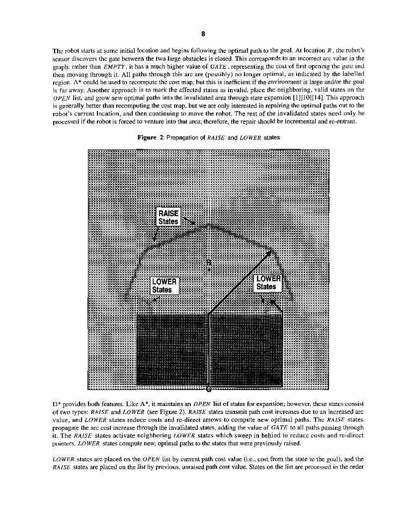
The robot starts at some initial location and begins following the optimal path to the goal. At location R I the robot’s sensor discovers the gate between the two large obstacles is closed, This corresponds to an incorrect arc value in the graph: rather than EMPTY, it has a much higher value of G A T E , representing the cost of first opening the gate and then moving through it. All paths through this arc are (possibly) no longer optimal, as indicated by the labelled rcgion. A* could be used to recompute the cost map, but this is inefficient if the environment is large and/or the goal is far away. Another approach is to inark the affected states as invalid, place the neighboring, valid states on the OPEN list. and grow new optimal paths into the invalidated area through state expansion [l][lO][l4]. This approach is generally better than recomputing the cost map, but we are only interested in repairing the optimal paths out to the robot’s current location, and then continuing to move the robot. The rest of the invalidated states need only be processed if the robot is forced to venture into that area; therefore, the repair should be incremental and re-entrant.

Figure 2: Propagation of RAISE and LOWER states

D* provides both features. Like A*, it maintains an OPEN list of states for expansion; however. these states consist of two types: RAISE and LOWER (see Figure 2). RAISE states transmit path cost increases due to an increased arc value, and LOWER states reduce costs and re-direct arrows to compute new optimal paths. The RAISE states propagate the arc cost increase through the invalidated states, adding the value of GATE to all paths passing through i t . The RAISE states activate neighboring LOWER states which sweep in behind to reduce costs and re-direct pointers. LOWER states compute new. optimal paths to the states that were previously raised.

LOWER states are placed on the OPEN list by current path cost value (i-e., cost from the state to the goal), and the R.4ISE states are placed on the list by previous. unraised path cost value. States on the list are processed i n the order

9

of increasing value. The intuition is that the previous optimal path costs of the RAISE states define a lower bound on the path costs of LOWER states they can discover. Thus. if the path costs of the LOWER states currently on the OPEN list exceed the previous path costs of the RAISE states, then it is worthwhile processing RAISE states to discover (possibly) a better LOWER state. Note in the figure that the arrow from the goal to the RAISE state wave front is equal in length to the arrow to the LOWER state wave front.

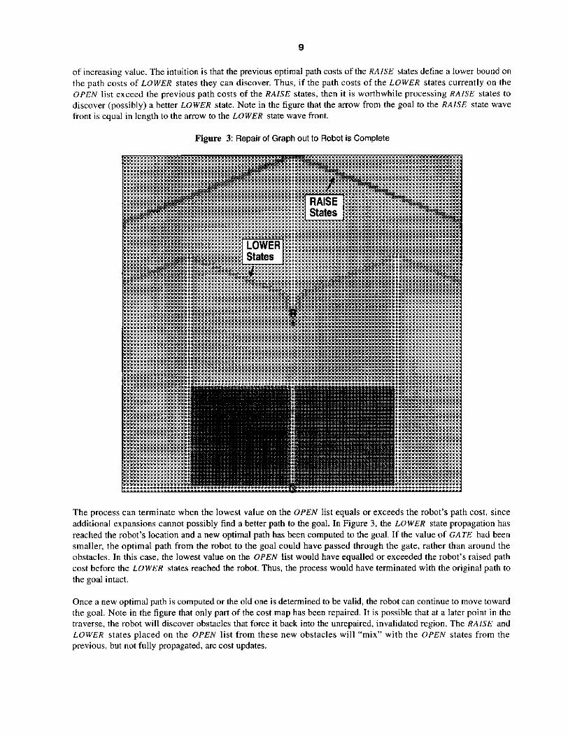
Figure 3: Repair of Graph out to Robot is Complete

The process can terminate when the lowest value on the OPEN list equals or exceeds the robot’s path cost, since additional expansions cannot possibly find a better path to the goal. In Figure 3, the LOWER state propagation has reached the robot’s location and a new optimal path has been computed to the goal. If the value of GATE had been smaller. the optimal path from the robot to the goal could have passed through the gate, rather than around the obstacles. In this case, the lowest value on the OPEN list would have equalled or exceeded the robot’s raised path cost before the LOWER states reached the robot. Thus, the process would have terminated with the original path to the goal intact.

Once a new optimal path is computed or the old one is determined to be valid, the robot can continue to move toward the goal. Note in the figure that only pan of the cost map has been repaired. It is possible that at a later point in the traverse, the robot will discuver ubstacles that force it back into the unrepaired, invalidated region. The RAlSE and LOWER states placed on the OPEN list from these new obstacles will ‘‘mix’’ with the OPEN states from the previous, but not fully propagated, arc cost updates.

10

D* supports multiple, partially-propagated cost updates by sorting the states on the OPEN list by the minimum of-all path cost values assumed hy the state immediately before insertion on the OPEN list and while resident on the list. Thus, RAISE and LOWER states propagate cost increases and reductions, respectively, from the lowest to highest path cost value in the map, regardless of the order in which arc cost corrections are made and the extent to which they are propagated. It is even possible for LOWER states to become RAISE states and vice versd in the process. If the robot ventures into a previously invalidated region, the algorithm propagates all cost updates logged to that point into this region to compute a new optimal path to the goal.

2.2 Definitions To formalize this intuition, we introduce the following notation and definitions. The problem space can be formulated as a set of stares denoting robot locations connected by directional am, each of which has an associated cost. The robot starts at a particular state and moves across arcs (incurring the wst of traversal) to other states until it reaches the goal state, denoted by G . Every state X except G has a backpointer Io a next state Y denoted by b(X) = Y . D' uses backpointers to represent paths to the goal. The cost of traversing an arc from state Y to state X is a positive number given by the arc cosr function c(X, n , If Y does not have an arc to X , then c(X. Yj is undefined. Two states X and Y are neighbors in the space if c(X, y) or c(Y, XI is defined.

Like A*, D* maintains an OPEN list of states. The OPEN list is used to propagate information ahout changes to the arc cost function and to calculate path costs to states in the space. Every state X has an associated tug rG7. such that r ( X ) = NE\+' if X has never been o n the OPEN list, t(X) = OPEN if X is currently on the OPEN list, and t(x) = CLOSED if X is no longer on the OPEN list. For each state X. D* maintains an estimate of the sum of the arc costs from X to G given by the pafh cosf function h(G, X ) . Given the proper conditions, this estimate is equivalent to the optimal (minimal) cost from state X to G . For each state X on the OPEN list (i.e., f t X ) = O P E N ) , the key function, k(G, X j , is defined to be equal to the minimum of h(F, X j before modification and all values assumed by h(G, X ) since X was placed on the OPEN list. The key function classifies a state X on the OPEN list into one of two types: a RAISE state if k(G, XI < h(C, X j , and a LOWER state if k(G, X j = h(G, X j , D* uses RAISE states on the OPEN list to propagate information about path cost increases and LOWER states to propagate information about path cost reductions. The propagation takes place through the repeated removal of states from the OPEN list. Each time a state is removed from the list, it is expanded to pass cost changes to its neighbors. These neighbors are in turn placed on the OPEN list to continue the process.

States o n the O P E N list are sorted by their key function value. The parameter k m i n is defined to be min(k(X)j for all X such that r ( X j = O P E N . The parameter kmin represents an important threshold in D*: path costs less than or equal to kn, in are optimal, and those greater than kmin may not be optimal. The parameter ko,d i s defined to be equal to kmln prior to most recent removal of a state from the OPEN list. If no states have been removed, k,, ld is undefined.

An ordering of states denoted by { X , , X J is defined to be a sequence if b(Xi+ = Xj for all i such that I < ;< N and Xi # X, for a11 (id7 such that 1 5 i j < N . Thus, a sequence defines a path of backpointers from X,,, to X , . A sequence [X,,X,,j is def ined to be monotonic if ( r ( X J = CLOSED and h ( G , X i ) < h ( G . X i + , j ) o r ( f ( X i ) = OPEN a n d k(C, Xi) < h(G. Xj+ for all i such that 1 5 i < N . D* constructs and maintains a monotonic sequence {G,W , representing decreasing current or lower-bounded path costs. for each state X that is or was on the OPEN list. Given asequenceofstates [ X , , X , J , s t a t ex i isanancestorofstateX, if l~ i<jI .Nandadescendanrofx . if 1 S j c i 5 N

Fur two-slate functions involving the goal state, the following shorthand notation is used: h ( m h(G, X ) and k(X) k(G, x) . Likewise, for sequences the notation (X) = [GX) is used. The notation f i " j is used to refer to a function independent of its domain.

2.3 Algorithm Description The Basic D* algorithm consists primarily of two functions: PROCESS-STATE and MODIFY- C O S T . PROCESS -STATE is used to compute optimal pathcosts to the goal, and M O D I F Y - C O S T is used to change the arc cost function c("j and enter affected states on the OPEN list. The algorithms for PROCESS-STATE and MODIFY- C O S T are presented below. The embeddedroutines are MIN(a, 6 ) , which returns the minimum of the two Scalar values a and b; LESS(0, bj , which returns TRUE if a is less than b and FALSE otherwise; COST(X) I which returns 1 1 0 7 for state X : M I N - S T A T E , which returns the state on the OPEN list with minimum k(") value (NULL if

I

11

the list i s empty); MIA'- V A L , which returns kmin for the O P E N list ( N O - VAL if the list is empty): DELETEIX), which deletes state X from the OPEN l i s t and sets r(X) = C L O S E D ; and INSERnX, h n e w ) , which computes k ( X ) = / I , , ~ ~ if r(m = N E W , k(X) = M/N(k(X) , hn,J if r(X) = O P E N . and !dx) = MIN(h(X), hnew) if r ( X ) = C L O S E D , sets h(X) = hnew and t(X) = O P E N . and places or re-positions state X on the OPEN list sorted by k(")

The function names LESS and COST are used rather than < and h ( " ) . respectively, since their semantics are redefined in Section 3.3 to operate on vectors rather than scalars.

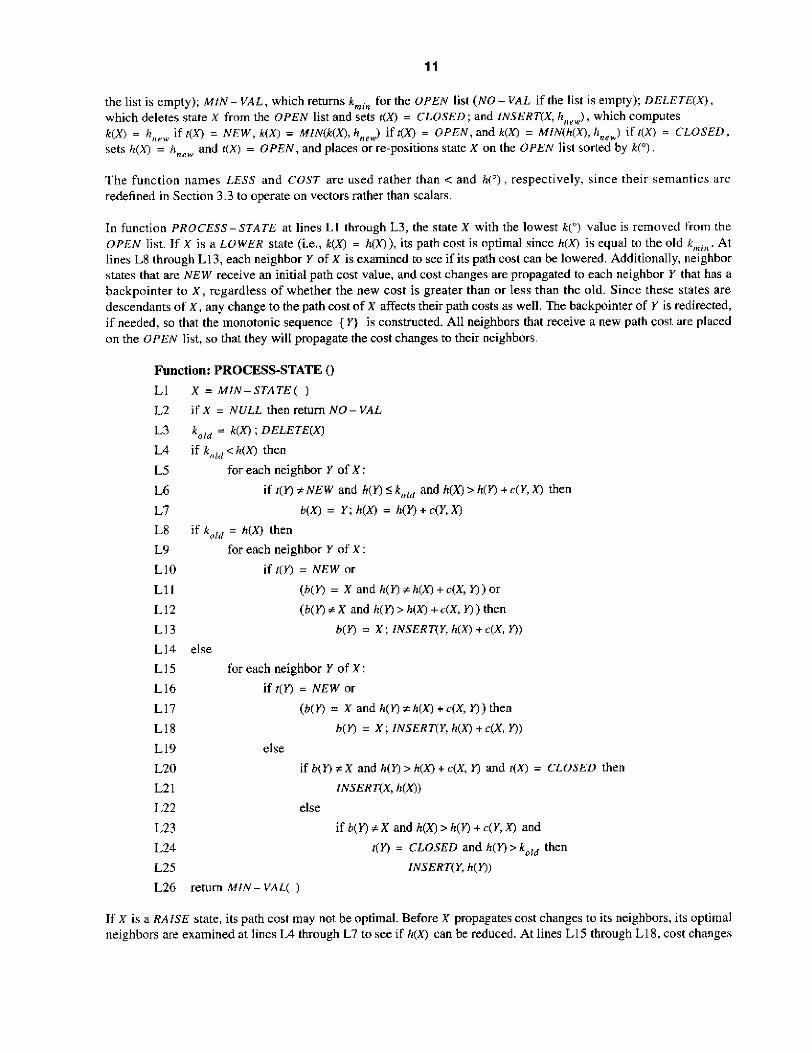
In function PROCESS-STATE at lines LI through L3, the state X with the lowest k(") value is removed from the OPEN list. If X is a LOWER state (Le., k ( X ) = h(X)). its path cost is optimal since h(X) i s equal to the old k,nin. At lines L8 through L13, each neighbor Y of X is examined to see if its path cost can be lowered. Additionally, neighbor states that are NEW receive an initial path cost value, and cost changes are propagated to each neighbor Y that has a backpointer to X , regardless of whether the new cost is greater than or less than the old. Since these states are descendants of X . any change to the path cost of X affects their path costs as well. The backpointer of Y is redirected, if needed, so that the monotonic sequence { Y ) is constructed. All neighbors that receive a new path cost are placed on the OPEN list, so that they will propagate the cost changes to their neighbors.

Function: PROCESS-STATE 0 L1 X = M I N - S T A T E ( )

L2 L3 k o l d = k ( X ) ; DELETE(X)

if X = NULL then return N O - VAL

LA if k ~ t l d < h ( x ) then L5 L6

for each neighbor Y of X :

if r ( Y ) #NEW and h(Y) 5 kold and h(Xj > h ( n + c(Y, x) then

L l b(X) = Y ; h(X) = h(Y) + c(Y, X j

L8 L9 L10 L11 ( b ( 0 = X a n d h ( Y ) t h ( X ) + c ( X , Y l ) o r L12 ( b ( Y ) t X andh(Y)>h(x)+c(X,Y))then

L14 else L15

L16 L17 ( b ( n =Xandh(Y)#h(X)+c(X,Yl)then

L19 else L20 L2 1 /NSERT(X, h(X))

L22 else L23 i fb (Y) tX andh(X)>h(Y)+c(Y,X) and

L24

if keld = NX) then for each neighbor Y of X :

if r(Y) = NEW or

LI 3 b(Y) = X; INSERT(Y, h(X) + c(X, Y))

for each neighbor Y of X :

if r ( Y ) = NEW or

L18 b(Y) = X ; INSERT(Y, h ( X ) + c(X, Y))

if b ( n # X and h(Yl > h(X) + c(X, Y) and t ( X ) = CLOSED then

r(Y) = CLOSED and h(Y) > kord then L25 INSERT(Y, h(Y))

L26 return MIN- VAL( )

If X is a RAISE state, its path cost may not be optimal. Before X propagates cost changes tu its neighbors, its optimal neighbors are examined at lines LA through L7 to see if h(X) can be reduced. At lines L E through L18, cost changes

12

are propagated to NEW states and immediate descendants in the same way as for LOWER states. If X is able to lower the path cost of a state that is not an immediate descendant (lines L20 and LZI), X is placed back on the OPEN list for future expansion. This action is required to avoid creating a closed loop in the backpointers [ 121. If the path cost of X is ahle to be reduced by a suboptimal neighbor (lines L23 through L25), the neighbor is placed hack on the OPE,\' list. Thus, the update is "postponed" until the neighbor has an optimal path cost. To assist the reader i n understanding this cos t propagation process, a simplified but less computationally efficient version of P R O C E S S - S T A T E is included in the Appendix.

In function M O D I F Y - C O S T , the arc cost function is updated with the changed value. Since the path cost for state Y will change. X is placed on the OPEN list. When X is expanded via P R O C E S S - S T A T E , it computes a new h(Y) = / r ( X ) + c ( X , v) and places Y on the OPEN list. Additional state expansions propagate the cost to the descendants of Y

Function: MODIFY-COST (X, Y, cval) LI c(X, 0 = cvaf

L2 L3 return W I N - VAL( )

if r ( x ) = CLOSED then INSERT(X, h(x))

The function M O V E -ROBOT illustrates how to use PROCESS-STATE and MODIFY - COST to move the robot from state S through the environment to G along an optimal traverse. At lines LI through L3 of M O V E - R O B O T . rt") is set to NEW for all states, h(G) is set to zero, and G is placed on the OPEN list. PROCESS-STATE is called repeatedly at lines L5 and L6 until either an initial path is computed to the robot's state (Le.. r ( 3 = C L O S E D ) or i t is determined that no path exists ( i c , vol = N O - VAL and (3 = N E W ) . The robot then proceeds to follow the hack- pointers in the sequence { R ) until it either reaches the goal or discovers a discrepancy (lines L10 and L11) between the .wnsor measurement of an arc cost s(0) and the stored arc cost c(") (e.g., due to a detected obstacle). Note that these discrepancies may occur anywhere, not just in the sequence { R } , MODIFY - COST is called to correct c(0) and place affected states on the OPEN list. PROCESS-STATE is then called repeatedly at line L13 until u u l t h ( R ) to propagate costs and compute a possibly new sequence { R ) to the goal. The robot continues to follow the back- pointers i n the sequence toward the goal. The function returns G O A L - REACHED if the goal is found and NO - PATH if it is unreachable.

Function: MOVE-ROBOT ( S , G ) L l for each state X in the graph: L2 r ( X ) = NEW

L3 /NSERT(C, 0)

L4 V a l = 0

L5 L6 " 0 1 = PROCESS-STATE( )

while r(S) # CLOSED and volt NO - VAL

L7 L8 R = S

L9 LlO LII L12 L13 ,,a1 = PROCESS-STATE( )

L14 R = b(R)

if tis) = NEW then return N O - PATH

while R # C : for each ( X , n such that s(X , Y) # c(X, n :

ual = MODIFY - COST(X, Y, s(X, Y))

while LESS(vaf , COST(.?)) and val # NO - VAL

L15 return G O A L - R E A C H E D

13

11 should be noted that line L l in M O V E - ROBOT only detects the condition that no sequence of arcs exists from the robot's state to the goal, if for example, the graph i s disconnected. It does not detect the condition that all paths to the goal are obstructed by obstacles. In order to provide for this capability. obstructed arcs can be assigned a large positive value of OBSTACLE and unobstructed arcs can be assigned a small positive value of E'MPTY. OBSTACLE should k chosen such that it exceeds the longest possible sequence of EMPTY arcs in the graph. No unobstructed path exists to the goal from S if h(S) > OBSTACLE after exiting the loop at line L5. Likewise, no unobstructed path exists to the goal from a state R during the traverse if h(R) t OBSTACLE after exiting the loop at line L12.

14

3.0 The Focussed D' Algorithm

3.1 Intuition

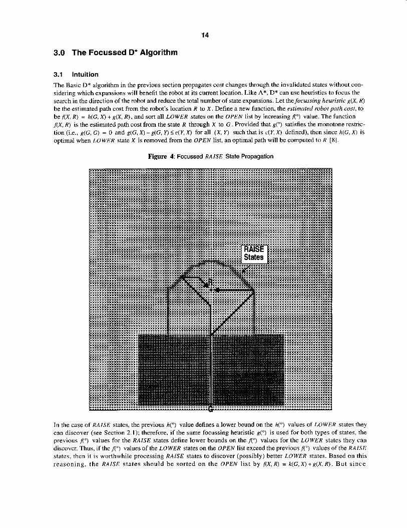
The Basic D* algorithm in the previous section propagates cost changes through the invalidated states without con- sidering which expansions will benefit the robot at its current location. Like A*, D* can use heuristics to focus the search in [he direction of the robot and reduce the total number of state expansions. Let the focusink. heuristic gLY R) be the estimated path cost from the robot's location R to X . Define a new function. the estimated robot path cost, to be AX. R ) = h(G. X) + g(X. R ) , and sort all LOWER states on the OPEN list by increasing r) value. The function JX, R) is the estimated path cost from the state R through X to G . Provided that g(") satisfies the monotone reshic- tion (Le., g(G, G ) = 0 and g(G. - g(G, l7 < c(Y, XI for all (X, u) such that is c(Y. X ) defined), then since k(C, A I is optimal when LOWER state X is removed from the OPEN list. an optimal path will be computed to R [SI

Figure 4: Focussed RAISE State Propagation

In the case of RAISE states, the previous h(") value defines a lower bound on the h(") values of LOWER states they can discover (see Section 2.1); therefore, if the same focussing heuristic g(0) is used for both types of states, the previous A") values for the RAISE states detine lower bounds on the f(") values for the LOWER states they can discuver. Thus, if the fl") values of the LOWER states on the OPEN list exceed the previous A') values of the R A U E states, then i t is wurthwhile processing RAISE states to discover (possibly) better LOWER states. Based on this r eason ing , the RAISE s ta tes should h e sor ted on the OPEN l i s t by f l X , R ) = k l G , X ) + g [ X , R ) . But s ince

15

k(G, ,-q = /t(G, x) for LOWER states, the RAISE state definition for A’) suffices for both kinds of states. To avoid cycles in the backpointers, it should be noted that ties in A“) are sorted by increasing k(”) on the O P E N list [12].

The process can terminate when the lowest value on the OPEN list equals or exceeds the robot‘s path cost, since the subsequent expansions cannot possibly find a LOWER state that 1) has a low enough path cost, and 2) is “close” enough to the robot to be able to reduce the robot’s path cost when it reaches it through subsequent expansions. Note that this is a more efficient cut-offthan the one outlined in Section 2.1, which considers only the first criterion.

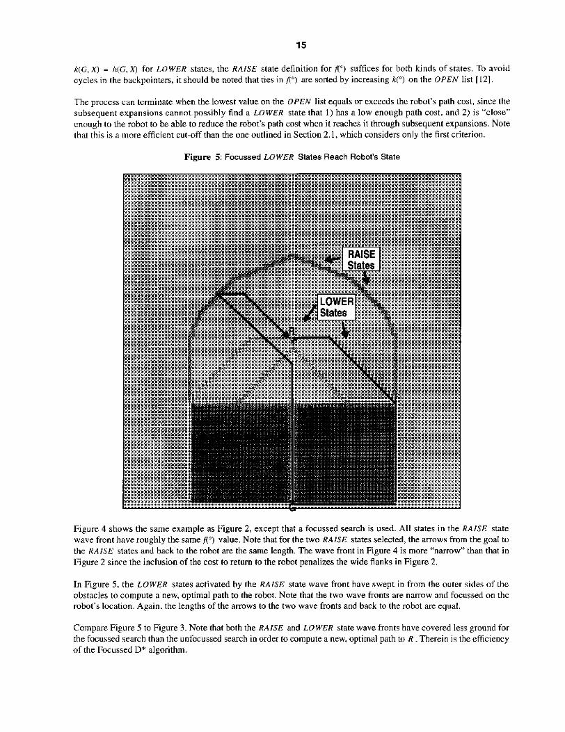
Figure 5: Focussed LOWER States Reach Robot’s State

Figure 4 shows the same example as Figure 2, except that a focussed search is used. All states in the RAISE state wave front have roughly the same A”) value. Note that for the two RAISE states selected, the arrows tiom the goal to the RAISE states and back to the robot are the same length. The wave front in Figure 4 is more “narrow” than that in Figure 2 since the inclusion of the cost to return to the robot penalizes the wide flanks in Figure 2.

In Figure 5, the LOWER states activated by the RAISE state wave front have swept in from the outer sides of the obstacles to compute a new. optimal path to the robot. Note that the two wave fronts are narrow and focussed on the robol’s location. Again. the lengths of the arrows to the two wave fronts and back to the robot are equal.

Compare Figure 5 to Figure 3. Note that both the RAISE and LOWER state wave fronts have covered less ground for the focussed search than the unfocussed search in order tocompute a new. optimal path to R . Therein is the efliciency of the Focussed D* algorithm.

16

The problem with focussing the search is that once a new optimal path is computed to the robot's location, it then moves to a new location. If the robot's sensor discovers another arc cost discrepancy, the search should be focussed on the robot's new location. But states already on the OPEN list are focussed on the old location and have incorrect 8(') and j ( ' ) values. One solution is to recompute g(") and fl") for all states on the OPEN list every time the robot moves and new states are to be added via MODIFY- COST. This approach is inefficient since it re-sorts the OPEN list, requiring at worst II(NlogM operations, where N is the number of states on the OPEN list. Based on empirical evidence, this additional computation more than offsets the savings gained by a focussed search.

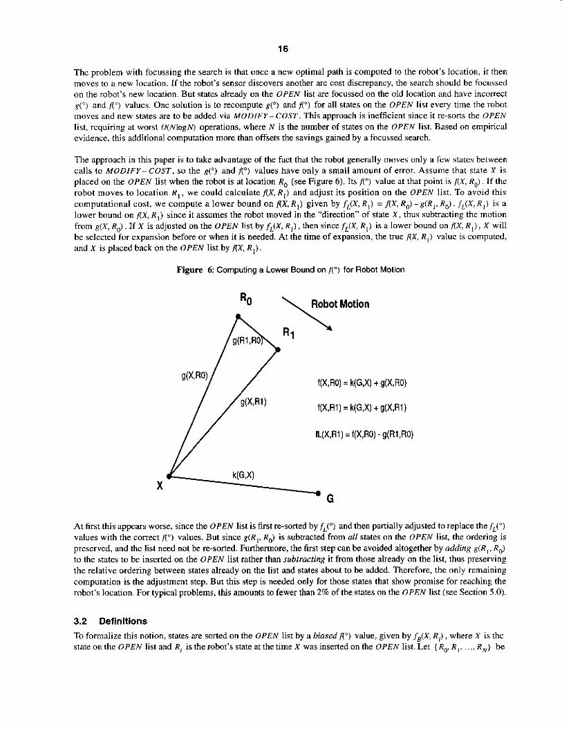
The approach in this paper is to take advantage of the fact that the robot generally moves only a few states between calls to MODIFY- COST, so the g(") and ft") values have only a small amount of error. Assume that state X is placed on the OPEN list when the robot is at location Ro (see Figure 6). Its fl") value at that point is fcX. Ro) , If the robot moves to location R I 1 we could calculate f l X , R , ) and adjust its position on the OPEN list. To avoid this computational cost, we compute a lower bound on AX, R 1 ) given by f L ( X , R 1 ) = A X . Ro) -g(RI. R J . J,(X. R , ) is a lower bound on A X , R 1 ) since it assumes the robot moved in the "direction" of state X. thus subtracting the motion fmm g(X, R J . If X is adjusted on the OPEN list by f L ( X , R l ) , then since f L [ X , R , ) is a lower bound on fixl R I j I X will be selected for expansion before or when it is needed. At the time of expansion, the true fix. R , ) value is computed, and X is placed back on the OPEN list by fix, R , ) .

Figure 6 Computing a Lower Bound on ft") for Robot Motion

RO Robot Motion

R1

f(X,RO) = k(G,X) t g(X.RO)

f(X,Ri) = k(G,X) t g(X,Ri)

fL(X,Ri) = f(X,RO) - g(R1,RO)

X * G

At first this appears worse. since the OPEN list is first resorted by f f ) and then partially adjusted to replace the JL("j values with the correct fl") values. But since g ( R 1 , Ro) is subBacted from nll states on the OPEN list, the ordering is preserved. and the list need not he re-sorted. Furthermore, the first step can be avoided altogether by adding g(R,, RJ to the states to be inserted on the OPEN list rather than subtracting it from those already on the list, thus preserving the relative ordering between states already on the list and states about to be added. Therefore, the only remaining computation is the adjustment step. But this step is needed only for those states that show pmmise for reaching the robot's locdtion. For typical problems, this amounts to fewer than 2% of the states on the OPEN list (see Section 5.0).

3.2 Definitions To formalize this notion, states are sorted on the OPEN list by a biased fl ') value, given by f B ( X , Ri), where X is the state on the OPEN list and Ri is the robot's state at the time X was inserted on the OPEN list. Let { Ro, R , . , . ., R,,J be

17

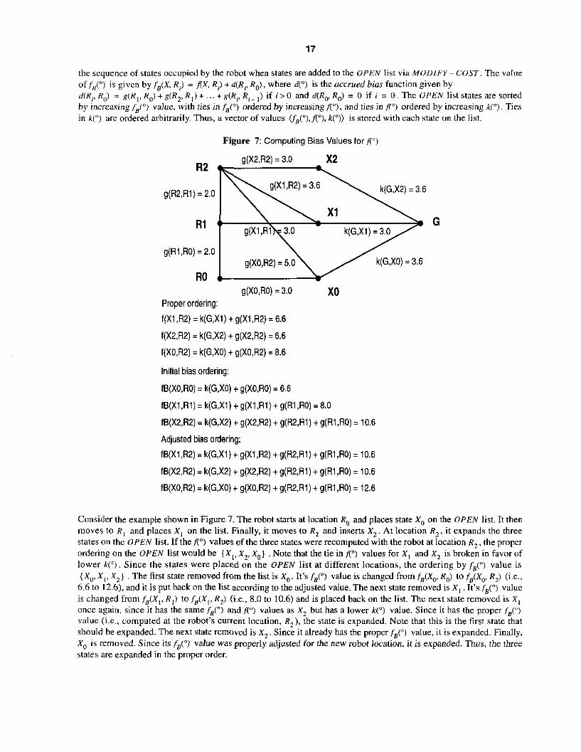
[he sequence of states occupied by the robot when states are added to the OPEl\' list via .MODIFY- C O S T , The value of f,,C"j is given by f B ( X , Rij = AX, R J + d(Ri; R o ) . where dpj is the accrued bias function given by d lR iRJ = g ( R 1 , R n ) + g ( R , , R I ) + ...+ g ( H i , R i ~ , j if i > O andd(Rn,Rn) = 0 if i = 0 . T h e U P E N liststatesaresorted by increasing f B P ) value, with ties in fJ0) ordered by increasing fl"), and ties in f7') ordered by increasing ki"). Ties in k(" ) are ordered arbitrarily. Thus, a vector of values (f,pj,T), W j ) is stored with each sVdte on the list.

Figure 7 Computing Bias Values for X'j

G

g(R1,RO) = 2.0

g(X2,RZ) = 3.0

g ( ~ 2 , ~ i ) '* = 2.0 K \ G , X 2 ) g(X1 ,R2) = 3.6 = 3.6

g(R1,RO) = 2.0 g(XO,R2) = 5.0 k(G,XO) = 3.6

RO xo g(X0,RO) = 3.0

Proper ordering:

f(X1,RZ) = k(G,Xl) tg(Xl,R2)=6.6

f(X2,R2) = k(G,X2) t g(X2,RZ) = 6.6

f(X0,RZ) = k(G,XO) t g(XO,R2) = 8.6

Initial bias ordering:

fB(X0,RO) = k(G,XO) t g(XOR0) = 6.6

fB(X1,Rl) = k(G,Xl) t g(X1,Rl) + g(R1,RO) = 8.0

fB(X2,RZ) = k(G,X2) t g(X2,RZ) t g(R2,Rl) t g(R1,RO) = 10.6

Adjusted bias ordering:

fB(X1,RZ) = k(G,Xl) t g(X1,RZ) + g(R2,Rl) t g(R1,RO) = 10.6

fB(X2,RZ) = k(G,X2) t g(X2,RZ) + g(R2,Rl) t g(R1,RO) = 10.6

fB(X0,RZ) = k(G,XO) + g(XO,R2) + g(R2,Rl) + g(R1,RO) = 12.6

Ccinsider the example shown in Figure 7. The mbot starts at location Rg and places state Xu on the OPEN list. It then moves to R , and places X, on the list. Finally, it moves to R , and inserts X 2 . At location R 2 . it expands the three states on the OPEN list. If the A") values of the three states were recomputed with the robot at location R , , the proper ordering on the OPEN list would be {X,, X2, xo} . Note that the tie in A") values for XI and X, is broken in favor of lower k(?. Since the states were placed on the OPEN list at different locations, the ordeiing by fBpj value is {Xo, X I ; X,} . The first state removed from the list is X,. It's f,p) value is changed fmm fB(Xo, Ruj to f,(X,, R,) (i.e., 6.6 to 12.61, and it is put back on the list according to the adjusted value. The next state removed is XI . It's f B ( " ) value is changed from f,(XI, R,) to f,CX,, R,) (i.e., 8.0 to 10.6) and is placed back on the list. The next state removed is X, once again. since i t has the same f,O and A") values as X 2 but has a lower k(") value. Since it has the proper f,(O)

value (Le., computed at the robot's current location, R , ) , the state is expanded. Note that this is the first state that should be expanded. The next state removed is X, , Since it already has the proper f,r) value, it is expanded. Finally, Xo is rrrnoved. Since its fB?) value was properly adjusted for the new mbot location, it is expanded. Thus, the three states are expanded in the proper order.

18

For a graph reprcsenting an eight-connected Cartesian amay of locations, a good focussing heuristic that satisfies the monotone restriction is the minimum arc distance heuristic. If the Cartesian array is indexed by (i, j ) , let (x i . xi) be the (i. j ) coordinates of state X. Let Cmfn be the minimum c(") cost in the array. after all arc costs are normalized to the length of a non-diagonal arc. Let d i be ki - yil and di be bj - yjl . Then g(X, V = Cmtn[ h d l + d , - dl 1 if df 2 d, and g ( X , V = C,,,,[ A d , + dj - d f ) if d i < dj .

Let Rcur, be the most recent robot state at which discrepancies were discovered between the sensor data and map, and let R,,,<, be the previous such state. Both are initialized to the robot's start state. Define the robot sfute function dx). which returns the robot's state when X was last inserted or adjusted on the OPEN list. The parameter dcarr is the accrued bias from the robot's start state to its current state; it is shorthand for d(Rcur,, KO) and is initialized to dca,, = d(Ro, R& = 0. Let fmin be the minimum fl") value on the OPEN list and kva, be its corresponding k(") value. The fo l lowing shorthand notation is used for far) , A"), and g r ) : fJX, =f,(X. r ( x ) ) , f l X , =fix. d W ) . and g(x) = g(X, dx))

3.3 Algorithm Extension Most of the extensions are confined to the functions for cost comparisons and management of the OPEh' list; there- fore. the functions C O S T . L E S S , INSERT, MIN-STATE, and M I N - VAL are affected. Instead ofreturning h(R) for a robot state R . COST(R) returns the vector of values (AR, RCuJ h(R)) .Instead ofcomparing two scalars, the function LESS(a, b) takes a vector of values ( a , , a*) for u and a vector ( b l , b2) fo rb . LESS returns TRUE if aI < b , or (0, = h , and u 2 < b r ) ; otherwise, it returns FALSE

Before redefining INSERT, M I N - S T A T E , and M I N - V A L , two new embedded functions a re introduced. PL'T-STATE(x) sets r ( x ) = OPEN and inserts X on the OPEN list according to the vector ((#),AX), k ( X ) ) , and G E T - S T A T E returns the state on the OPEN list with minimum vector value (NULL if the list is empty).

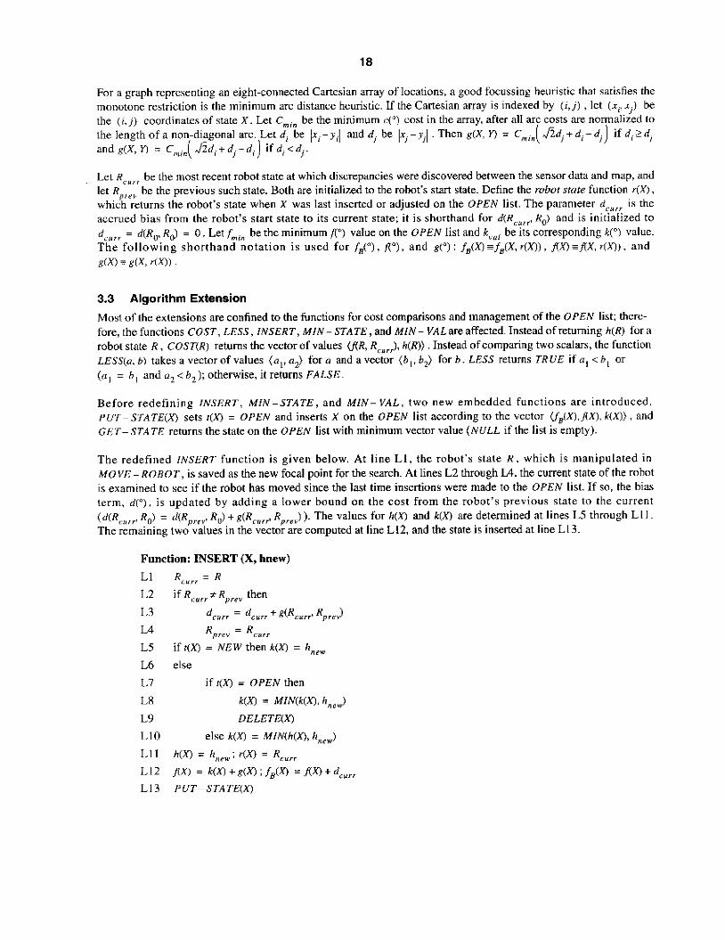
The redefined /NSERT function is given below. At line L1, the robot's state R . which is manipulated i n MOVE- R O B O T , is saved as the new focal point for the search. At lines L2 through LA, the current state of the robot i s examined to see if the robot has moved since the last time insertions were made to the OPEN list. If so, the bias term, d(") , is updated by adding a lower bound on the cost from the robot's previous state to the current (d(RCAA,? , Ro) = d(Rprrr . R O ) + g(Rcu7, Rp,J ). The values for h ( x ) and k(X, are determined at lines L5 through LI I The remaining two values in the vector are computed at line L12, and the state is inserted at line L13.

Function: INSERT (X, hnew)

L1 R<;w,r = R L2 L3

if Rcur , # Rprev then

dcarr = dcxrr + R(Rcur,: Rpr.$

L4 Rprev = Rc",r L5 L6 else L7

L8 k(X) = MIN(k(x), h,,J LY DELETE(X)

L10

if r(X, = NEW then k ( X ) = haew

if t(m = OPEN then

else k(X) = MIN(h(X), h,,J

L11 h(x) = r(x) = Rcur,

L12 L13 PUT-STATE(x)

fix, = k(X) +g(W ; ,f,W = AX) + dcu,,

19

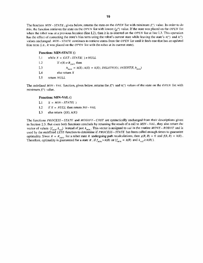
The function .Mihr-STATE, given below, returns the state on the OPEN list with minimum /Yj value. In order lo do this, the function retrieves the state on the OPEN list with lowest f8r) value. If the state was placed on the OPEN list when the robot was at a previous location (line L2). then it is re-inserted on the OPEN list at line 13. This operation has the effect of correcting the state's bias term using the robot's current state while leaving the state's It(") and k(") values unchanged MIN - STATE continues to retrieve states from the O P E N list until it finds one that has an updated bias term (i,e,, it was placed on the O P E N list with the robot at its current state).

Function: MIN-STATE 0 I,I L2

L3 L4 else return X

L5 return NULL

while X = GET-STATE( ) # N U L L

if r(x) # Rcu,r then

hncw = h(W; h(Xj = k(W; DELETE(-; lNSERT(X, h>,*,J

The redefined M I N - VAL function, given below, returns the A") and k(") values of the state on the OPEh' list with minimum (("j value.

Function: MIN-VAL 0 LI x = M f N - S T A T E ( )

L2

L3 else return MW, k(W)

if X = NULL then return NO - VAL

The functions PROCESS-STATE and M O D I F Y - COST are syntactically unchanged from their descriptions given in Section 2.3. But since both functions conclude by returning the result of a call to MIAr- V A L , they also return the vector of \ d u e s {fmin, k,,"J instead ofjust k m i n . This vector is assigned to val in the routine M O V E - ROBOT and is used by the redefined LESS function to determine if PROCESS-STATE has been called enough times to guarantee optimality. Since R = Ret,,, for a robot state R undergoing path recalculations, then g(R, R) = 0 and AR, R ) = h K . Therefore, optimality is guaranteed for a state R ~ if fmin > h(R) or (fmim = h(Rj and k,n , Z h(R) ).

20

4.0 Examples

This scctian presents two examples that illuseate the operation of the D* algorithm. The first compares the Basic D* algorithm to Focussed D*, and the second compares planning with complete information to optimistic information.

4.1 D' Comparisons

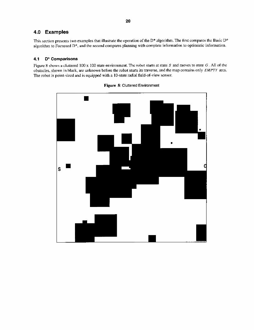
Figure 8 shows a cluttered 100 x 100 state environment. The robot starts at state S and moyes to state G . All of the obstacles, shown in black, are unknown before the robot starts its traverse, and the map contains only E M P T Y arcs. The robot is point-sized and is equipped with a 10-state radial field-of-\' 'lew sensor.

Figure 8: Cluttered Environment

I ,.

I

21

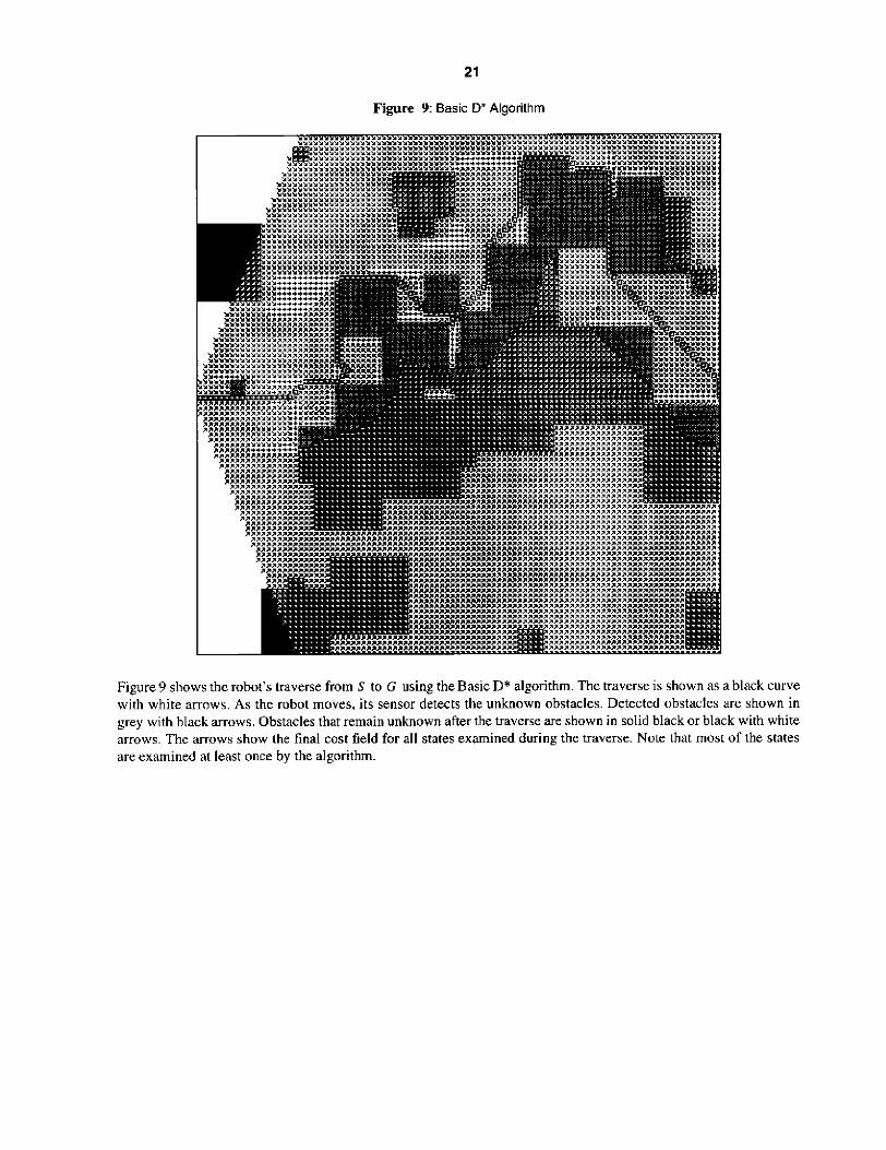
Figure 9: Basic D' Algorithm

Figure 9 shows the robot's traverse from S to G using the Basic D* algorithm. The traverse is shown as a black curve with white arrows. As the robot moves. its sensor detects the unknown obstacles. Detected obstacles are shown in grey with black arrows. Obstacles that remain unknown after the traverse are shown in solid black or black with white arrows. The arrows show the final cost field for a11 states examined during the traverse. Note that most of the states are examined at least once by the algorithm.

22

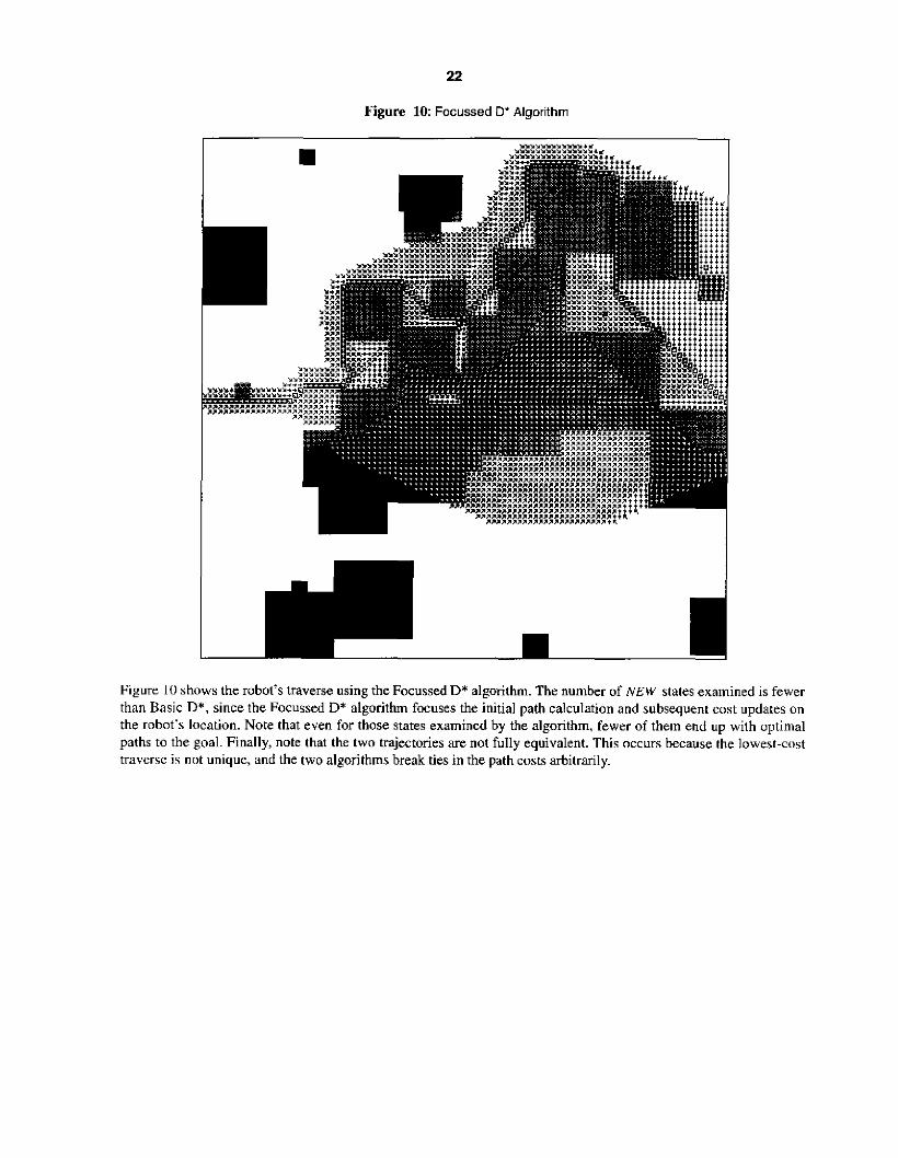
Figure 10 Focussed 0' Algorithm

i Figure 10 shows the robot's traverse using theFocussedD* algorithm. The number of NEW states examined is fewer than Basic D*. since the Focussed D* algorithm focuses the initial path calculation and subsequent cost updates on the robot's location. Note that even for those states examined by the algorithm. fewer of them end up with optimal paths to the goal. Finally, note that the two trajectories are not fully equivalent. This occurs because the lowest-cost traverse is nut unique, and the two algorithms break ties in the path costs arbitrarily.

23

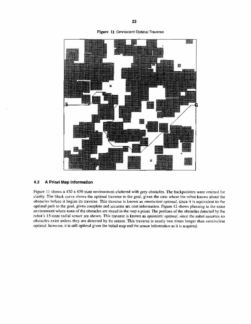
Figure 11: Omniscient Optimal Traverse

I

4.2 A Priori Map Information

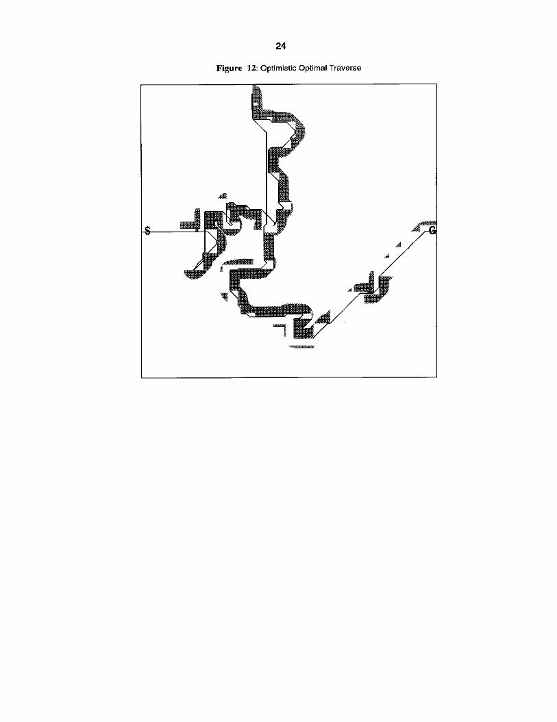
Figure 11 shows a 450 x 450 state environment cluttered with grey obstacles. The backpointers were omitted for clarity. The black curve shows the optimal traverse to the goal, given the case where the robot knows about the obstdcles before it begins its traverse. This traverse is known as omniscient optimal, since it is equivalent to the optimal path to the goal, given complete and accurate arc cost information. Figure 12 shows planning in the same environment where none of the obstacles are stored in the map a priori. The portions of the obstacles detected by the robot’s 15-state radial sensor are shown. This traverse is known as optimistic optimal, since the robot assumes no obstacles exist unless they are detected by its sensor. This traverse is nearly two times longer than omniscient optimal; however, it is still optimal given the initial map and the sensor information as it is acquired.

24

Figure 12: Optimistic Optimal Traverse

25

5.0 Experimental Results

Four algorithms were tested to verify optimality and to compare run-time and memory usage results. The first algorithm. the Brute-Force Replanner (BFR), initially plans a single path from the goal to the start state. The robot proceeds tu td low the path until its sensor detects an error in the map. The robot updates the map, plans a new path from the goal to its current location using a focussed A* search [SI, and repeats until the goal is reached. The fi)cussing heuristic used is the minimum arc distance described in Section 3.2.

The second and third algorithms, Basic D* (BD*) and Focussed D* with Minimal Initialization (FD*M). are described in Sections 2.0 and 3.0, respectively. The fourth algorithm, Focussed D* with Full Initialization (FD*F). is the same as FD*M except that the path costs are propagated to all states in the planning space, which is assumed to be finite, during the initial path calculation, rather than terminating when the path reaches the robot’s start state.

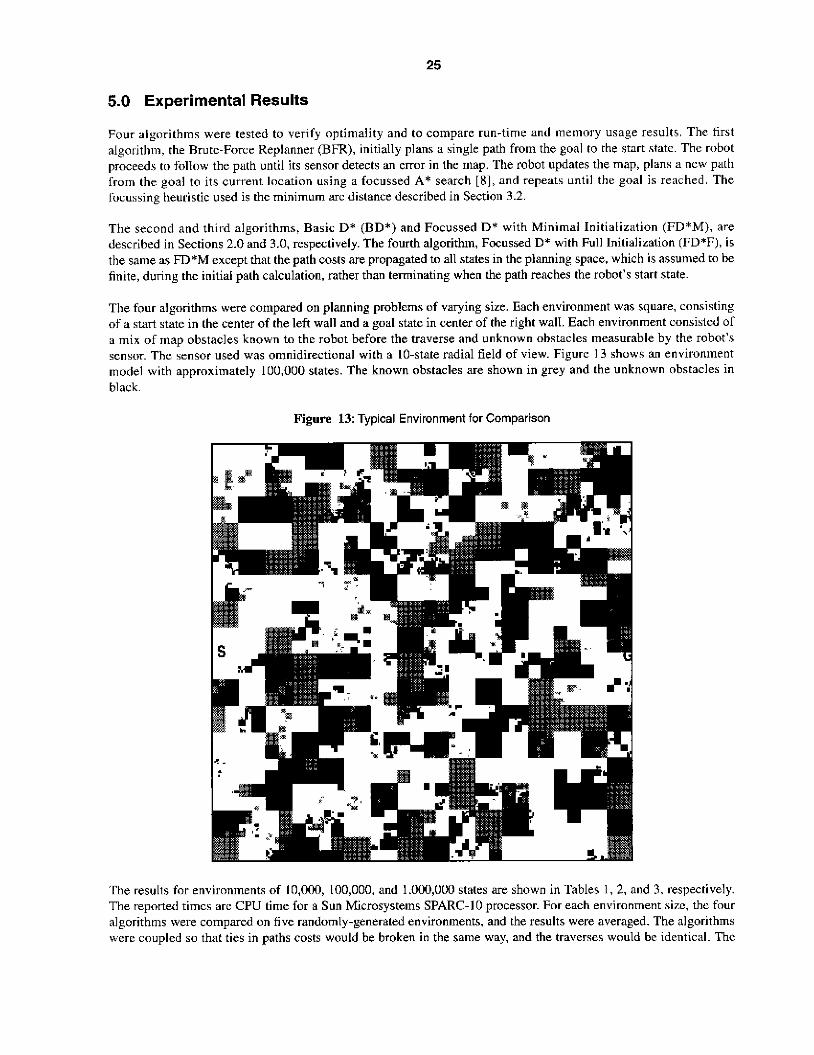
The four algorithms were compared on planning problems of varying size. Each environment was square. consisting ofa start state in the center of the left wall and a goal state in center of the right wall. Each environment consisted of a mix of map obstacles known to the robot before the traverse and unknown obstacles measurable by the robot’s sensor. The sensor used was omnidirectional with a IO-state radial field of view. Figure 13 shows an environment model with approximately 100,000 states. The known obstacles are shown in grey and the unknown obstacles in black.

Figure 13: Typical Environment for Comparison

The results for environments of 1O.Oo0, 100,000. and 1,0D3,000 states are shown in Tables 1, 2. and 3, respectively. The r e p i e d times are CPU time for a Sun Microsystems SPARC-10 processor. Fnr each environment size. the four algorithms were compared on five randomly-generated environments, and the results were averaged. The algorithms were coupled so that ties in paths costs would be broken in the same way? and the traverses would be identical. Thc

26

Off-line Time

On-line Time

Memory %

On-line %

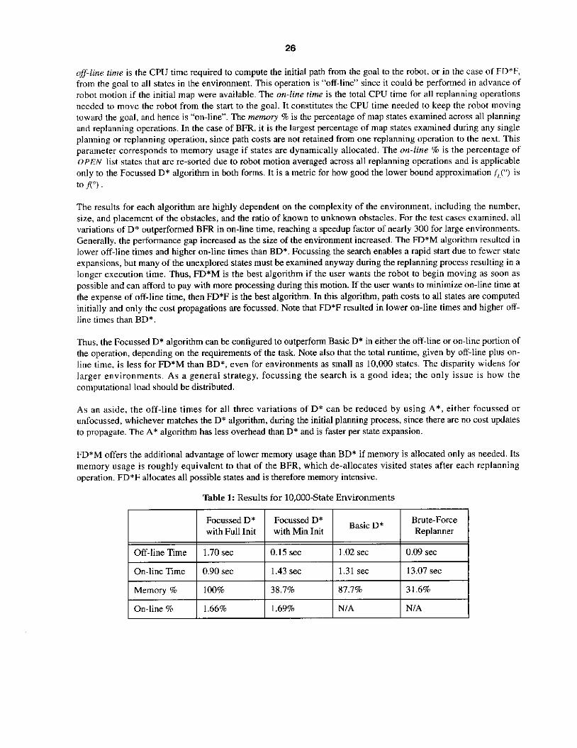
off-line time is the CPU time required to compute the initial path from the goal to the robot, or in the case of FD*F, from the goal to all states in the environment. This operation is “off-line” since it could be performed i n advance of robot motion if the initial map were available. The on-line rim is the total CPU time for all replanning operations needed to move the robot from the start to the goal. I t constitutes the CPU time needed to keep the robot moving towmard the goal, and hence is “on-line”. The memory % is the percentage of map states examined across all planning and replanning operations. In the case of BFR, it is the largest percentage of map states examined during any single planning or replanning operation, since path costs are not retained from one replanning operation to the next. This parameter corresponds to memory usage if states are dynamically allocated. The on-line % is the percentage of O P E N list states that are re-sorted due to robot motion averaged across all replanning operations and is applicable only to the Focussed D* algorithm in both forms. It is a metric for how good the lower bound approximation f,?) is to A”) .

The results for each algorithm are highly dependent on the complexity of the environment, including the number, size. and placement of the obstacles, and the ratio of known to unknown obstacles. For the test cases examined. all variations of D* outperformed BFR in on-line time, reaching a speedup factor of nearly 300 for large environments. Generally. the performance gap increased as the size of the environment increased. The FD*M algorithm resulted in lower off-line times and higher on-line times than BD*. Focussing the search enables a rapid start due to fewer state expansions, but many of the unexplored states must be examined anyway during the replanning process resulting in a longer execution time. Thus, FD’M is the best algorithm if the user wants the robot to begin moving as soon as possible and can afford to pay with more processing during this motion. If the user wants to minimize on-line time at the expense of off-line time, then FD*F is the best algorithm. In this algorithm, path costs to all states are computed initially and only the cost propagations are focussed. Note that FD*F resulted in lower on-line times and higher otf- line times than BD’.

Thus, the Focussed D* algorithm can be configured to outperform Basic D* in either the off-line or on-line portion of the operation, depending on the requirements of the task. Note also that the total runtime, given by off-line plus on- line lime. is less for FD*M than BD*, even for environments as small as 10,OOO states. The disparity widens for larger environments. As a general strategy, focussing the search is a good idea; the only issue is how the computational load should be distributed.

As an aside. the off-line times for all three variations of D* can be reduced by using A*, either focussed or unfocussed. whichever matches the D* algorithm, during the initial planning process, since there are no cost updates to propagate. The A* algorithm has less overhead than D* and is faster per state expansion.

FD*M offers the additional advantage of lower memory usage than BD* if memory is allocated only as needed. Its memory usage is roughly equivalent to that of the BFR, which de-allocates visited states after each replanning operation. FD*F allocates all possible states and is therefore memory intensive.

Table 1: Results for 10,000-State Environments

Brute-Force Basic D* Focussed D* Focussed D* with Full Init with Min Init Replanner

1.70 sec 0.15 sec I .02 sec 0.09 sec

0.90 sec 1.43 sec 1.31 sec 13.07 sec

100% 38.7% 87.7% 31.6%

1.66% 1.69% NIA NIA

27

Off-line Time

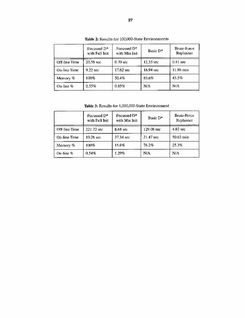
Table 2: Results for 100,000-State Environments

Brute-Force Replanner Basic D* Focussed D* Focussed D*

with Full Init with Min Init

20.58 sec 0.70 sec 12.55 sec 0.41 sec

Basic D* Focussed D* Focussed D* with Full Init with Min Init

Off-line Time 221.72 sec 8.68 sec 129.08 SK

I On-line Time I 9.22 sec I 17.62 sec I 16.94sec I 11.86min I

Brute-Force Replanner

4.82 sec

I Memory& 1100% I 50.4% I 83.6% I 43.5% I 1 On-line % I 0 3 % I 0.85% I NIA I NIA I

1 On-line Time I 10.26 sec I 37.34 sec I 21.47 sec I 50.63 min I I Memory% I 100% I 15.6% I 76.2% I 25.3% I I On-line% I 0 5 4 % I 1.29% I NtA I NfA I

28

6.0 Conclusions

This paper presents the D* algorithm for rea-time path replanning. The algorithm computes an initial path from the goal state to the start state and then efficiently modifies this path during the traverse as arc costs change. The algorithm is guaranteed to produce an optimal traverse. meaning that an optimal path to the goal is followed at every state in the traverse, assuming all known information at each step is correct. D* i s far more efticient than the brute- force path planner. The focussed version of D* outperforms the basic version, and it offers the user the option of distributing the computational load amongst the on- and off-line portions of the operation. depending on the task requirements. Furthermore, the focussed version can be configured to be less memory intensive and is therefore better for large environments.

D* is a very general algorithm and can be applied to problems in artificial intelligence other than robot motion planning. In its most general form. D* can handle any path cost optimization problem where the cost parameters change during the traverse of the solution. D* is most efficient when these changes are detected near the current starting point in the search space, which i s the case with arobot equipped with an on-board sensor.

Acknowledgments The author thanks Barry Brumitt and Jay Gowdy for feedback on the use of the algorithm and the entire Unmanned Ground Vehicle (UGV) project at CMU for providing a vehicle testbed.

29

References [ l ] Bonlt. T., “Updating Distance Maps when Objects Move”, Proc. of the SPlE Conference on Mobile Robots. 1987. [21 Goto. Y.. Stentz. A,. “Mobile Robot Navigation: The CMU System”. IEEE Expert, Vol. 2, No. 4, Winter, 1987. [31 Jarvis. K. A., “Collision-Free Trajectory Planning Using the Distance Transforms”. Mechanical Engineering Trans. of the Institution of Engineers. Australia; Vol. MElO. No. 3, September. 1985. 141 Koti, R. E., “Real-Time Heuristic Search: First Results”, Proc. Sixth National Conference on Artificial Intelli- gence; July, 1987. 151 I-atombe. J.X., “Robot Motion Planning”, Kluwer Academic Publishers, 199 I 161 Lozano-Perez. T.. “Spatial Planning: A Configuration Space Approach, IEEE Transactions on Computers, Vol. C-32, No. 2, February, 1983. [71 Lumelsky, V. J . , Stepanov, A. A., “Dynamic Path Planning for aMobile Automaton with Limited Information o n the Environment”. IEEE Transactions on Automatic Control, Vol. AC-3 I , No. I I , November. 1986. [SI Nilsson. N. J., “Principles of Artificial Intelligence”, Tioga Publishing Company, 1980. 191 Pirzadeh. A.? Snyder. W., “A Unified Solution to Coverage and Search in Explored and Unexplored Terrains Using Indirect Control”. Proc. of the IEEE International Conference on Robotics and Automation, May, 1990. [ I O ] Rainalingam. G . , Reps. T.. “An Incremental Algorithm for a Generalization of the Shortest-Path Problem”. Uni- versity of Wisconsin Technical Repon#1087, May. 1992. [ I 11 Samet. H., “An Overview of Quadtrees, Octrees and Related Hierarchical Data Structures”, in NATO AS1 Series, Vo. F40, Theoretical Foundations of Computer Graphics, Berlin: Springer-Verlag, 1988. [I21 Stentz, A.. “Optimal and Efficient Path Planning for Unknown and Dynamic Environments”. Carnegie Mellon Robotics Institute Technical Report CMU-RI-TR-93-20. August, 1993. [I31 Stentz, A.. “Optimal and Efficient Path Planning for Partially-Known Environments”. Proc. of the IEEE Interna- tional Conference on Robotics and Automation, May. 1994. [141 Trovato, K. I., “Differential A*: An Adaptive Search Method Illustrated with Robot Path Planning for Moving Obstacles and Goals, and an Uncertain Environment”, Journal of Pattern Recognition and Artificial Intelligence. Vol. 1. No. 2. 1990. 11.51 Zelinsky, A.. “A Mobile Robot Exploration Algorithm”, IEEETransactions on Robotics and Automation. Vol. 8, No. 6. December, 1992.

30

Appendix

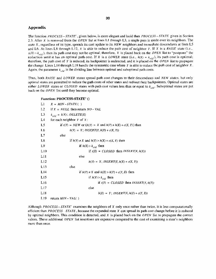
The function PROCESS-STATE’ . given below, is more elegant and lucid than PROCESS-STATE given in Section 2.3. After X is removed from the OPEN list at lines LI through L3, a single pass is made over its neighbors. The state X. regardless of its type. spreads its cost update to its NEW neighbors and immediate descendants at lines L5 a d Lh. At lines L8 through L12, X is able to reduce the path cost of neighbor Y . If X is a R A I S E state (i.e.: /iX) > k , , l d ) , then its path cost may not be optimal; therefore, X is placed hack on the OPEN list lo “pustpone” the reductiun until i t has an optimal path cost. If X is a LOWER state [i.e.$ h(X) = k P l d ) , its path cost is optimal; therefore. the path cost of Y is reduced. its backpointer is redirected, and it is placed on the OPEN list to propasate the change. Lines L14 through L18 handle the symmetric case where Y is able to reduce the path cost of neighbor X . Again: the parameter kr,ld is the dividing line between optimal and suboptimal path cosw.

Thus, both RAISE and LOWER states spread path cost changes to their descendants and NEW states. hut cinly optimal states are permitted to reduce the path costs of other states and redirect their hackpointers. Optimal stales are either LOWER states or CLOSED states with path cost values less than or equal to k p l d . Suboptimal states are put back on the OPEN list until they become optimal.

Function: PROCESS-STATE’ () L1 X = M I A - S T A T E ( )

L2 L3

L4 L5 ifr(n =NEWor(b(Yj = Xandh(Y)#h(X)+c(X.n)then

if X = NULL then return NO- VAL

k,,,,, = k ! x ) ; DELETE(x) for each neighbor Y of X:

L6 L7 else L8 L9 LIO L11 L12 L13 L14 L15 L16 LI 7 L18 L19 return M I N -

if b ( n # X and h ( n > h(X) + c(X, 0 then if h(X) > k,,, then

else if r [ x ) = CLOSED then lNS.kRT(X, h(mj

b(YJ = X. INSERT(Y, h(X) + c(X. n) else

i f b ( n # X a n d h [ ~ > h ( n + c ( Y , X ) then if h(n > k,,,d then

else if r(n = CLOSED then INSERT!Y, /I( i‘))

b(x) = Y . I N J E R q X , h(n + c(Y, a) VAL! j

Although PROCESS-STATE‘ examines the neighbors of X only once rather than twice, i t is less computationally efticient than P R O C E S S - S T A T E , because the expanded state X can spread its path cost change before it is reduced by optimal neighbors. This condition is detected, and X is placed back on the OPEN list to propagate the correct values. These additional OPEN list insertions are expensive compared to the cost of examining a state’s neighbors more than once.