IEEE TRANSACTIONS ON AUTOMATIC CONTROL, VOL. AC-31, NO. 8, AUGUST 1986 77 1

Pu

Fig. 2. Piecewise nonlinear perturbation.

1 1.0 1.0 *.o ..O r c

(a) I.0 I . O .A 4.0

(b)

- F

7, ( 0 LrMwwJwA2wm p-__-I-_ 3 . 0 t - D 3.0 *.e

( C)

=

(d) Fig. 3. (a) and (b) are the unit step responses ofy , ( t ) andyz(l) by (15) choosing k, =

0.3. (c) and (d) are the unit step responses ofyl(t) and y2(t) by another PI controller, without considering the robust stabilization

In the time domain, the unit step responses yl(t) and y*(t) with kl = 0.3 [shown in Fig. 3(a) and (b)] are better than the simulated results using a PI controller tuned with the unit-step tracking [shown in Fig. 3(c) and (d)] which does not consider the robust stability constraint (10).

VI. SUMMARY AND CONCLUSION

In this note we have considered the robustness of the stability property of MIMO feedback systems subjected to time-varying nonlinear perturba- tions. Moreover, a simple and direct controller design algorithm has been introduced to synthesize robust stabilizers which ensure that practical feedback systems will always remain stable in the face of variations in system models. In particular, we extend the nonlinear perturbation to systems with unstable plants.

REFERENCES

J. C. Doyle and G. Stein, “Multivariable feedback design: Concepts for a classicallmodem synthesis,” IEEE Trans. Automat. Contr., vol. AC-26, pp. 4- 16. Feb. 1981. D. C. Youla, H. A. Jabr, and J. J. Boniorno, Jr., “Modern Wiener-Hopf design of optimal controllers-Part U: The multivariable case,” IEEE Trans. Automat. Contr., vol. AC-21, pp. 319-338, June 1976. J . B. Cmz, Jr., J . S . Freudenixrg, and D. P. Looze, “A relationship benveen sensitivity an stability of multivariable feedback systems,” IEEE Trans. Automat. Contr., vol. AC-26, pp. 66-74, Feb. 1981. N. R. Sandell, Jr., “Robust stability of systems with application to singular perturbations,” Automatics. vol. 15, pp. 476480, July 1979. C. A. Desoer, R. W. Liu, J . Murray, and P. Saeks, “Feedback system design:

Automot. Contr., vol. AC-25, pp. 399420, June 1980. The fractional representation approach to analysis and synthesis,” IEEE Trans.

PH. Delsarte, Y. Genin, and Y. Kamp, “Schur parametrization ofpositive definite lilock-to e p k system,” SIAM J. Appl. Math., vol. 26, Feb. 1979. M. I. Chen and C. A. Desoer, “Necessary and sufficient condition for robust stability oflinear distributed feedbacksystem,” Int. J. Contr.. vol. 35, no. 2, pp. 255-267, 1982. M. G. Safonov and M. Athans, ”A multiloop generalization of the circle criterion for stability margin analysis,” IEEE Trans. Automat. Contr., vol. AC-26, pp. 415422. Apr. 1981.

I. W. Sandberg, “On the b-boundedness of solutions of nonlinear functional equations,” Bell Syst. Tech. J. , vol. 43, pt. U, pp. 1581-1599, July 1964. I. W. Sandberg, “A frequencydomain condition for the stability of feedback systems containing a single time-varying nonlinear element,” Bell Syst. Tech. J. , vol. 43, pp. 1601-1608, 1984. G. Zames, “On the input output stability of time-varying nonlinear feedback system-Part I: Conditions derived using concepts of loop gain, conicity, and positivity,” IEEE Trans. Automat. Contr., vol. AC-11, pp. 228-239, Apr. 1966. G. Zames, “On the input output stability of time-varying nonlinear feedback system-Pan n: Conditions involving circles in the frequency plane and sector nonlinearities,” IEEE Trans. Automat. Contr., vol. AC-11, pp. 465476, July 1966. T. Kailath, Linear Systems. Englewood Cliffs, NJ: Prentice-Hall, 1980.

The Consumption-Tracking Theory of Macroeconomic Systems

GUO BAOPING

Abstract-A new discrete-time dynamic input-output economic model, the consumption-tracking model, is proposed. This model combines dynamic input-output analysis with modern control techniques. The system objective function is a consumption-tracking criterion based on economic principles.

I. INTRODUCTION

Input-output analysis has been widely used as an analytical tool since it was developed by Leontief [l]. Now at least 80 countries have used the static input-output model for short-run forecasting, economic planning, and the analysis of economic development; and some countries have used the dynamic input-output model to analyze and describe a ma- croeconomy. However, these models did not incorporate optimal control techniques.

This note introduces a new model, combining dynamic input-output analysis with modem optimal control techniques, to obtain the consump- tion-tracking model.

In this note, Section I1 reviews various forms of Leontiefs original dynamic input-utput model including the important contributions of Luenberger and Arbel, Mickle and Vogt, and Sharp and Perkins in the last ten years. Section III presents the new input-output model, the consump tion-tracking model. Section N gives an illustration. Section V is further discussion.

n. REVIEW OF THE DYNAMIC INPUT-OUTPUT MODEL

The general n-dimension dynamic input-output model originally set forth 121 is

X,=AX,+B(X,Ll-X,)+ Y, (1)

where X , is the vector of production outputs, Y, is the final consumption vector, A is the production coefficient matrix, and B is the investment - flow matrix.

If the B matrix is nonsingular, then (1) has the forward recursive form

x,,, =B-’ [ (Z-A +B)X,- Y,]. (2)

Leontief developed this recursive form [3]. If (I - A + B) is

Manuscript received September IO, 1985; revised March 25, 1986. The author is m’ith the Administrative Commission, Tianjin Economic and Technologi-

IEEE Log Number 8609222. cal Development Area, Tianjin, China.

0018-9286/86/0800-0771~1.00 0 1986 IEEE

772 IEEE TRANSACTIONS ON AUTOMATIC CONTROL, VOL. AC-31, NO. 8, AUGUST 1986

nonsin,dar, then

X K = [ Z - A + B ] - ' [ B X K + I + YK].

Kendrick [4], Livesey [ 5 ] , and Luenberger and Arbel [6] introduced some forward recursive forms for (1). All of these approaches involve the partitioning of the B matrix.

Mickle and Vogt developed the Leontief dynamic input-output model which included excess demand and a feedback matrix 171. The Mickle- Vogt model is

xK+,=xK+FeK (3)

YK=(z-A)XK-BFeK (4)

eK= Y i - YK (5)

where Y, is the supply available for external consumption, Yi is the external demand, e is the excess external demand, and F is the feedback matrix.

The elements of the feedback matrix F are parameters which are empirically determined from the response time [A.

With a partitioning approach, Sharp and Perkins obtained the model as

where B I 1 , BI2 come from reordering B when B is singular

The first p elements of n-vectors U are the rate of change of capital stock in the first p sectors and the last n - p elements of the n-vector U are the rate of change of production in the last n - p sectors.

This model can be stabilized by appropriate selection of a feedback matrix.

A linear programming version of the dynamic input-output model has already been developed. But a quadratic optimal control criterion has not bee proposed.

m. THE CONSUMPTION-TRACKING THEORY Ah'D MODEL

In this model the macroeconomic system equation is based on the Sharp-Perkins model

where

If an appropriate objective function containing specific economic significance is added to this model, we obtain an optimal control model of a macroeconomy.

The author proposes the consumption-tracking control criterion as follows:

min J=- (Xv-Xtr)'S(X.v-Xd,) 1 2

where X;. is the ideal production output vector in N-year, and S, G , and R are the weight matrices.

This objective function is a discrete output-tracking model. So it is called the consumption-tracking model.

It is known that production is for consumption, the goal of investment is for future consumption, and the final goal of all production is in the end for external consumption. Generally, the supply Y and ideal demand Yd are not in equilibrium. A government planner tries to minimize this excess (excess = demand - supply). The above objective hnction reflects these thoughts.

The integrated consumption-tracking model is as follows:

1 2

min J = - ( X ~ - X ~ . ) S ( X , - X ~ , )

.x,- I

+? [( YK- Yi) 'G( YK- Y",+ UiRUK] (14) K = O

subject to:

X K + I = X K + H U K (15)

YK=(Z-A)XK-DUK (16)

x0 = 4 0 ,

(K=O, 1 , 2, ... N-1). (17)

This model can easily be solved by dynamic programming or by the maximum principle.

N. AN ILLUSTRATION

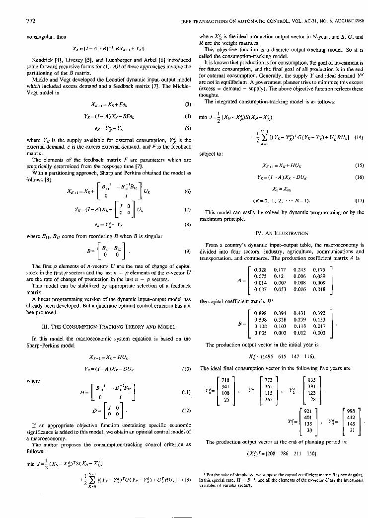
From a country's dynamic input-output table, the macroeconomy is divided into four sectors: industry, agriculture, communications and transportation, and commerce. The production coefficient matrix A is

0.328 0.171 0.243 0.175 0.075 0.12 0.006 0.039 0.014 0.007 0.008 0.009 0.037 0.053 0.016 0.018

A = [ 1 .[ 0.598 0.108 0.338 0.103 0.259 0.118 0.153 0.017 . I

the capital coefficient matrix B'

0.898 0.394 0.431 0.392

0.005 0.003 0.012 0.003

The production output vector in the initial year is

Xl=(1495 615 147 116).

The ideal final consumption vector in the following five years are

The production output vector at the end of planning period is:

(X!)'=[208 786 211 1501.

In this special case, H = B -', and a l l the elements of the n-\rector (I are the investment I For the sake of simplicity. we suppose the capital coefficient mamx B is nonsingular.

variables of various sectors.

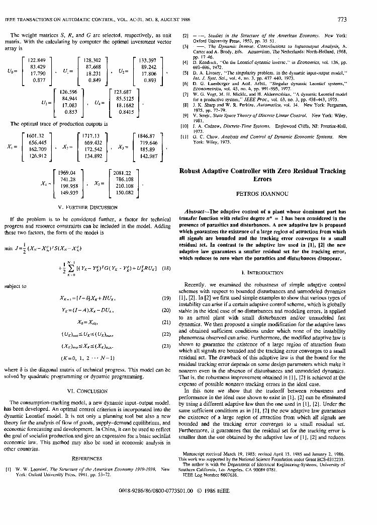
The weight matrices S, R , and G are selected, respectively, as unit matrix. With the calcuiating by computer the optimal investment vector array is

uo =

122.849 128.302 133.397 83 429 17:790 1 ’ ul= 1 18.231 1 ’ u2= [ 87.668 89.242

17.806 0.893 1 0.877 1

U, =

The optimal trace

x, =

1 0.849 1 126.596 [ : E ] ’ u,=

of production outputs is

1601.32 1

162.709 126.912

1 149.939 1

123.687 85.5125 18.1682 0.8415 I

717.13 1846.87 719.646

172.542 185.89 134.892 142.987

V. FURTHER DISCUSSION

If the problem is to be considered further, a factor for technical progress and resource constraints can be included in the model. Adding these two factors, the form of the model is

subject to

(K=O, 1, 2 ... N-1)

where 6 is the diagonal matrix of technical progress. This model can be solved by quadratic programming or dynamic programming.

VI. CONCLUSION

The consumption-tracking model, a new dynamic input-output model, has been developed. An optimal control criterion is incorporated into the dynamic Leontief model. It is not only a planning tool but also a new theory for the analysis of flow of goods, supply-demand equilibrium, and economic forecasting and development. In China, it can be used to reflect the goal of socialist production and give an expression for a basic socialist economic law. This method may also be used in economic analysis in other countries.

REFERENCES

[I] W. W . Leonrief, The Structure of the American Economy 1919-1939. New York: Oxford University Press, 1941, pp. 53-72.

Oxford University Press, 1953, pp. 35-53, -, Studies in the Structure of the American Economy. Neu, York:

-, The Dynamic Inverse. Contributions to Inputoutput Analysis, A. Caner and A. Brody, Eds. Amsterdam. The Netherlands: North-Holland, 1968, pp. 1746 . D. Kendrick, “On the Leontief dynamic inverse,” in Economics, vol. 136, pp.

D. A. Livesey, “The singularity problem. In the dynamic input-output model.”

D. G . Luenberger and A d . A r b e l . “Singular dynamic Leontief systems,” Int. J. Syst. Sci., vol. 4, no. 3, pp. 4 3 7 4 0 . 1973.

Econometrica, vol. 45, no. 4, pp. 991-995, 1977. W . G. Vogt, hl. H. Mickle, and H. Aldenneshian. “A dynamic Leontief model for a productive system,” IEEE Proc., vol. 63. no. 3. pp. 438-443, 1975. J. K. Sharp and W. R. Perkins, Automatica, vol. 14. Neu, York: Pergaman, 1975, pp. 77-79. V. Srrejc, State Space Theory of Discrete Linear Control. New York: Wiley, 198 I.

J . A. Cadzow. Discrete-Time Systems. Englewood Cliffs. NJ: Prentice-Hall. 1973.

693-696, 1972.

[ I l l G. C. Chow. Analysis and Control of Dynamic Economic Systems. New York: Wiley. 1975.

Robust Adaptive Controller with Zero Residual Tracking Errors

PETROS IOANNOU

IEEE TRANSACTIONS ON AUTOMATIC CONTROL, VOL. AC-31, NO. 8, AUGUST 1986 773

0018-9286/86/08OO-0773$01 .OO 0 1986 IEEE

Abstract-The adaptive control of a plant whose dominant part has transfer function with relative degree n* = 1 has been considered in the presence of parasitics and disturbances. A new adaptive law is proposed which guarantees the existence of a large region of attraction from which all signals are bounded and the tracking error converges to a small residual set. In contrast to the adaptive law used in [l], [2] the new adaptive law guarantees a smaller residual set for the tracking error, which reduces to zero when the parasitics and disturbances disappear.

I. INTRODUCTION

Recently, we examined the robustness of simple adaptive control schemes with respect to bounded disturbances and unmodeled dynamics [l], [2]. In [2] we first used simple examples to show that various types of instability can arise if a certain adaptive control scheme, which is globally stable in the ideal case of no disturbances and modeling errors, is applied to an actual plant with small disturbances andlor unmodeled fast dynamics. We then proposed a simple modification for the adaptive laws and obtained sufficient conditions under which none of the instability phenomena observed can arise. Furthermore, the modified adaptive law is shown to guarantee the existence of a large region of attraction from which all signals are bounded and the tracking error converges to a small residual set. The drawback of this adaptive law is that the bound for the residual tracking error depends on some design parameters which make it nonzero even in the absence of disturbances and unmodeled dynamics. That is, the robustness improvement obtained in [l] , [2] is achieved at the expense of possible nonzero tracking errors in the ideal case.

In this note we show that the tradeoff between robustness and performance in the ideal case shown to exist in [l], [2] can be eliminated by using a different adaptive law than the one used in [ I ] , [2]. Under the same sufficient conditions as in [ I ] , [2] the new adaptive law guarantees the existence of a large region of attraction from which all signals are bounded and the tracking error converges to a small residual set. Furthermore, it guarantees that the residual set for the tracking error is smaller than the one obtained by the adaptive law of [I]? [2] and reduces

This work was supported by the National Science Foundation under Grant ECS-8312233. Manuscript received March 19, 1985: revised April 15. 1985 and January 2, 1986.

Southern California, Los Angeles, CA 900894781. The author is with the Departmenr of Electrical Engineering-Systems, University of

IEEE Log Number 8607638.