Embed Size (px)
Citation preview

Consumption and Savings Decisions:A Two-Period Setting
Dynamic Macroeconomic Analysis
Universidad Autonoma de Madrid
Fall 2012
Dynamic Macroeconomic Analysis (UAM) Consumption and Savings Fall 2012 1 / 68

1 Summary
2 Credit marketsBudget constraintsPreferencesThe optimization problemComparative statics
Change in xInterest rate changes
The elasticity of intertemporal substitution
3 ExtensionsThe Life Cycle Hypothesis
4 Equilibrium with Many AgentsCredit Market EquilibriumA Numerical Example
Dynamic Macroeconomic Analysis (UAM) Consumption and Savings Fall 2012 2 / 68

Outline
In the first lecture we studied labor-leisure decisions in a staticenvironment.
In this lecture we study consumption and savings decisions in atwo-period setting. The original model was developed by Irving Fisher.
We consider a pure exchange economy. Agents receive a knownendowment of goods in both periods.
I Alternatively, we can think of an economy with inelastic labor supply.
The final good is perishable, but agents can borrow and lend on aperfectly competitive credit market.
There is still no money in the economy. No financial intermediationby banks either. Bonds are the only financial instrument.
Dynamic Macroeconomic Analysis (UAM) Consumption and Savings Fall 2012 2 / 68

Savings motives
Why do people save?
1 Consumption smoothing - agents dislike fluctuations in consumptionspending.
2 Precautionary motives — fear of unemployment etc.
3 Retirement
4 Purchase of real estate or durable consumption goods.
For the moment we focus on 1. Saving for retirement is treated at the endof the course, while precautionary savings is left for later.
Dynamic Macroeconomic Analysis (UAM) Consumption and Savings Fall 2012 3 / 68

Bonds
A bond is a piece of paper with a promise of a future payment of acertain amount of goods to the holder of the bond.
Bonds are issued by borrowers and handed over to lenders.
All bonds are supposed to expire in one period.
We denote the (real) interest rate by R.
A loan of 1 unit of the final good in period t implies a repayment of1 + R units of the final good in period t + 1.
We assume complete information. All loans are repaid.
Dynamic Macroeconomic Analysis (UAM) Consumption and Savings Fall 2012 4 / 68

Notation
Let bt denote the bond holdings of a household in period t
I Positive values bt > 0 imply that the household is a lender.
I On the contrary, when bt < 0 the household is a borrower.
The household that buys bt bonds in t will receive (1 + Rt)bt inperiod t + 1.
Since the credit market only operates between the first and secondperiod we drop the time index on R.
Dynamic Macroeconomic Analysis (UAM) Consumption and Savings Fall 2012 5 / 68

Budget constraints
In general terms, the one-period budget constraint of a household canbe written as
ct + bt = yt + (1 + R)bt−1
When bt−1 > 0, the resources of the household exceed the value ofincome
yt + (1 + R)bt−1 > yt
By contrast, when bt−1 < 0, the household has to devote part of thisperiod’s resources to pay back the loan plus interest
yt + (1 + R)bt−1 < yt
Dynamic Macroeconomic Analysis (UAM) Consumption and Savings Fall 2012 6 / 68
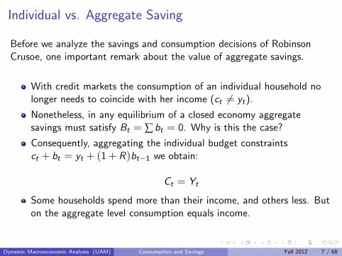
Individual vs. Aggregate Saving
Before we analyze the savings and consumption decisions of RobinsonCrusoe, one important remark about the value of aggregate savings.
With credit markets the consumption of an individual household nolonger needs to coincide with her income (ct 6= yt).
Nonetheless, in any equilibrium of a closed economy aggregatesavings must satisfy Bt = ∑ bt = 0. Why is this the case?
Consequently, aggregating the individual budget constraintsct + bt = yt + (1 + R)bt−1 we obtain:
Ct = Yt
Some households spend more than their income, and others less. Buton the aggregate level consumption equals income.
Dynamic Macroeconomic Analysis (UAM) Consumption and Savings Fall 2012 7 / 68

Robinson Crusoe in a Two-period Setting
In the rest of this theme, we analyze the case of an economy that lasts fortwo periods.
We start by analyzing the decisions of a single agent:
I Robinson receives an endowment (or fixed income) of y1 units in thefirst and y2 units in the second period.
I Robinson takes the interest rate as given and needs to choose hisconsumption and savings in both periods.
Dynamic Macroeconomic Analysis (UAM) Consumption and Savings Fall 2012 8 / 68

One-period budget constraints
Robinson faces the following pair of one-period budget constraints:
c1 + b1 = y1,
c2 + b2 = y2 + (1 + R)b1.
Robinson’s savings in the second period are necessarily equal to zero— He would like to borrow an infinite amount, but there are nolenders! Hence,
c2 = y2 + (1 + R)b1
Dynamic Macroeconomic Analysis (UAM) Consumption and Savings Fall 2012 9 / 68
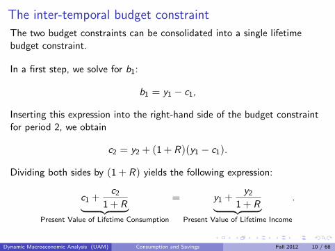
The inter-temporal budget constraint
The two budget constraints can be consolidated into a single lifetimebudget constraint.
In a first step, we solve for b1:
b1 = y1 − c1,
Inserting this expression into the right-hand side of the budget constraintfor period 2, we obtain
c2 = y2 + (1 + R)(y1 − c1).
Dividing both sides by (1 + R) yields the following expression:
c1 +c2
1 + R︸ ︷︷ ︸Present Value of Lifetime Consumption
= y1 +y2
1 + R︸ ︷︷ ︸Present Value of Lifetime Income
.
Dynamic Macroeconomic Analysis (UAM) Consumption and Savings Fall 2012 10 / 68
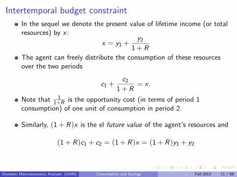
Intertemporal budget constraint
In the sequel we denote the present value of lifetime income (or totalresources) by x :
x = y1 +y2
1 + R
The agent can freely distribute the consumption of these resourcesover the two periods
c1 +c2
1 + R= x .
Note that 11+R is the opportunity cost (in terms of period 1
consumption) of one unit of consumption in period 2.
Similarly, (1 + R)x is the el future value of the agent’s resources and
(1 + R)c1 + c2 = (1 + R)x = (1 + R)y1 + y2
Dynamic Macroeconomic Analysis (UAM) Consumption and Savings Fall 2012 11 / 68
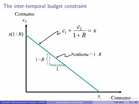
The inter-temporal budget constraint
Dynamic Macroeconomic Analysis (UAM) Consumption and Savings Fall 2012 12 / 68
Preferences
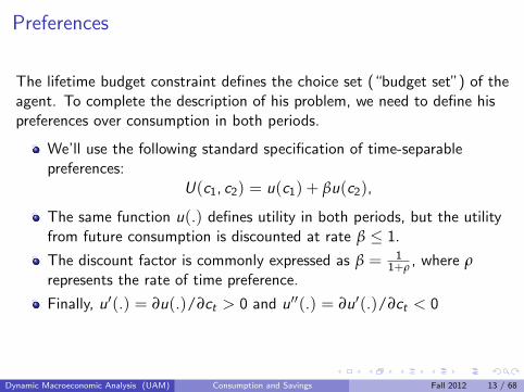
The lifetime budget constraint defines the choice set (“budget set”) of theagent. To complete the description of his problem, we need to define hispreferences over consumption in both periods.
We’ll use the following standard specification of time-separablepreferences:
U(c1, c2) = u(c1) + βu(c2),
The same function u(.) defines utility in both periods, but the utilityfrom future consumption is discounted at rate β ≤ 1.
The discount factor is commonly expressed as β = 11+ρ , where ρ
represents the rate of time preference.
Finally, u′(.) = ∂u(.)/∂ct > 0 and u′′(.) = ∂u′(.)/∂ct < 0
Dynamic Macroeconomic Analysis (UAM) Consumption and Savings Fall 2012 13 / 68
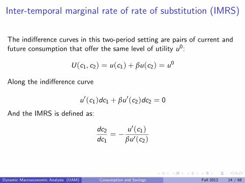
Inter-temporal marginal rate of rate of substitution (IMRS)
The indifference curves in this two-period setting are pairs of current andfuture consumption that offer the same level of utility u0:
U(c1, c2) = u(c1) + βu(c2) = u0
Along the indifference curve
u′(c1)dc1 + βu′(c2)dc2 = 0
And the IMRS is defined as:
dc2
dc1= − u′(c1)
βu′(c2)
Dynamic Macroeconomic Analysis (UAM) Consumption and Savings Fall 2012 14 / 68

Example
Throughout the course we will often use the example of logarithmicpreferences (“log-utility”):
u(c1, c2) = log(c1) + β log(c2).
These preferences satisfy our set of assumptions and often yield simpleclose-form solutions.
∂u(c1, c2)∂c1
=1
c1;
∂2u(c1, c2)∂c2
1
= − 1
c21
Dynamic Macroeconomic Analysis (UAM) Consumption and Savings Fall 2012 15 / 68
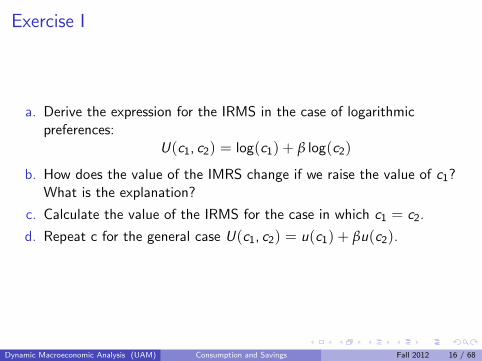
Exercise I
a. Derive the expression for the IRMS in the case of logarithmicpreferences:
U(c1, c2) = log(c1) + β log(c2)
b. How does the value of the IMRS change if we raise the value of c1?What is the explanation?
c. Calculate the value of the IRMS for the case in which c1 = c2.
d. Repeat c for the general case U(c1, c2) = u(c1) + βu(c2).
Dynamic Macroeconomic Analysis (UAM) Consumption and Savings Fall 2012 16 / 68

Answers
a. The total derivative is given by
1
c1dc1 +
β
c2dc2 = 0.
Hence,dc2
dc1= − c2
βc1
b. An increase in c1 causes a fall in the value of the IMRS. Marginalutility from consumption in the first period is decreasing in c1. Hence,an agent who consumes a large quantity of goods in the first periodand few goods in the second period, will be willing to sacrifice oneunit of first-period consumption in return for a small amount ofadditional consumption in the second period.
c. 1/β
d. Idem
Dynamic Macroeconomic Analysis (UAM) Consumption and Savings Fall 2012 17 / 68
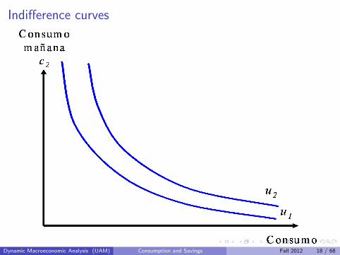
Indifference curves
Dynamic Macroeconomic Analysis (UAM) Consumption and Savings Fall 2012 18 / 68

The Optimization Problem of an Agent
In compact form the optimization problem can be written as
maxc1,c2
[u(c1) + βu(c2)] (1)
subject toc2
1 + R+ c1 = x . (2)
Like before there are two solution methods. Here we use thesubstitution method. Given that
c2 = (x − c1)(1 + R),
we can rewrite the maximand as
maxc1
[u(c1) + βu((x − c1)(1 + R))] (3)
Dynamic Macroeconomic Analysis (UAM) Consumption and Savings Fall 2012 19 / 68

The solution
The FOC associated with our optimization problem
maxc1
[u(c1) + βu((x − c1)(1 + R))]
is given by:
u′(c1) + βu′((x − c1)(1 + R)︸ ︷︷ ︸c2
)(−1)(1 + R) = 0.
Or alternatively,u′(c1)︸ ︷︷ ︸
MC
= u′(c2)β(1 + R)︸ ︷︷ ︸MB
u′(c1)βu′(c2)︸ ︷︷ ︸
IMRS
= 1 + R.
Dynamic Macroeconomic Analysis (UAM) Consumption and Savings Fall 2012 20 / 68

Graphical representation of solution
Dynamic Macroeconomic Analysis (UAM) Consumption and Savings Fall 2012 21 / 68
Consumption Euler equation
The optimality condition — known as the Consumption Euler equation —
u′(c1)βu′(c2)
= (1 + R)
is nothing else than the intertemporal variant of a well-known result inconsumption theory.
IMRS = price ratio of consumption in both periods
Dynamic Macroeconomic Analysis (UAM) Consumption and Savings Fall 2012 22 / 68
Optimal profile of consumption
According to the Euler equation
u′(c1) = β(1 + R)u′(c2)
there are two opposing forces that affect the inter-temporal choices of theagent
The stronger the degree of time preference — the lower is β —, theless attractive is c2;
The higher is the interest rate, the more attractive it is to save.
Dynamic Macroeconomic Analysis (UAM) Consumption and Savings Fall 2012 23 / 68

Perfect consumption smoothing
When β(1 + R) = 1, the Euler eqn. reduces to:
u′(c1) = u′(c2).
Given the strict concavity of u(.), this implies c1 = c2.
Intuition: Recall that β = 1/(1 + ρ). Hence, the necessary condition forperfect consumption smoothing can be written as:
β(1 + R) =1 + R
1 + ρ= 1,
which is only satisfied ifR = ρ.
Dynamic Macroeconomic Analysis (UAM) Consumption and Savings Fall 2012 24 / 68
Rising of falling consumption profiles
Using the same line of argument, one can easily demonstrate that theconsumption Euler eqn
u′(c1)βu′(c2)
= (1 + R)
implies the following three results
β(1 + R) < 1 =⇒ c1 > c2
β(1 + R) = 1 =⇒ c1 = c2
β(1 + R) > 1 =⇒ c1 < c2
The above conditions play a central role in any dynamic macro model withendogenous consumption choices.
Dynamic Macroeconomic Analysis (UAM) Consumption and Savings Fall 2012 25 / 68

Log utility
Suppose that the agent’s preferences satisfy
u(c1) + βu(c2) = log(c1) + β log(c2).
In this case, we can write the maximand as
maxc1
[log(c1) + β log((x − c1)(1 + R))]
and the associated FOC is:
1
c1+ β
1
c2(−1)(1 + R) = 0
1
c1=
1
c2β(1 + R) =⇒ c2 = β(1 + R)c1
c2
c1= β(1 + R).
Dynamic Macroeconomic Analysis (UAM) Consumption and Savings Fall 2012 26 / 68

Log Utility
In this particular case, it is straightforward to obtain closed-form solutionsfor the optimal consumption levels. Substituting c2 = β(1 + R)c1 into thelifetime budget constraint we get:
c1 +c1β(1 + R)
1 + R= x ,
And so,
(1 + β)c1 = x =⇒ c1 =x
1 + β.
c2 = c1β(1 + R) =β
1 + βx(1 + R).
b1 = y1 − c1 = y1 −x
1 + β=
1
1 + β
[βy1 −
y2
1 + R
]
Dynamic Macroeconomic Analysis (UAM) Consumption and Savings Fall 2012 27 / 68

Lagrange method
Let’s return to our original problem
maxc1,c2
[u(c1) + βu(c2)] (4)
subject toc2
1 + R+ c1 = x . (5)
The Lagrangian associated with the above maximization problem canbe written as:
L(c1, c2, λ) = u(c1) + βu(c2) + λ[x − c2
1 + R− c1]
Dynamic Macroeconomic Analysis (UAM) Consumption and Savings Fall 2012 28 / 68

Solution
L(c1, c2, λ) = u(c1) + βu(c2) + λ[x − c2
1 + R− c1]
The FOCs are given by:
∂L(c1, c2, λ)∂c1
= u′ (c1)− λ = 0
∂L(c1, c2, λ)∂c2
= βu′ (c2) + λ(− 1
1 + R) = 0
∂L(c1, c2, λ)∂λ
= x − c2
1 + R− c1 = 0
Using the fact that λ = u′ (c1), we obtain the same solution asbefore:
u′(c1)︸ ︷︷ ︸MC
= u′(c2)β(1 + R)︸ ︷︷ ︸MB
Dynamic Macroeconomic Analysis (UAM) Consumption and Savings Fall 2012 29 / 68
Comparative statics
Our next objective is to determine the response of the optimal solutions tochanges in x and R.
Let’s start with the case of an increase in x :
A rise in x represents a pure income effect that leads to an increase incurrent and future consumption;
The effect on borrowing or lending depends on the timing of the risein income;
Transitory and permanent changes produce different effects;
Dynamic Macroeconomic Analysis (UAM) Consumption and Savings Fall 2012 30 / 68
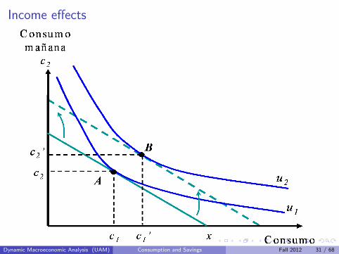
Income effects
Dynamic Macroeconomic Analysis (UAM) Consumption and Savings Fall 2012 31 / 68
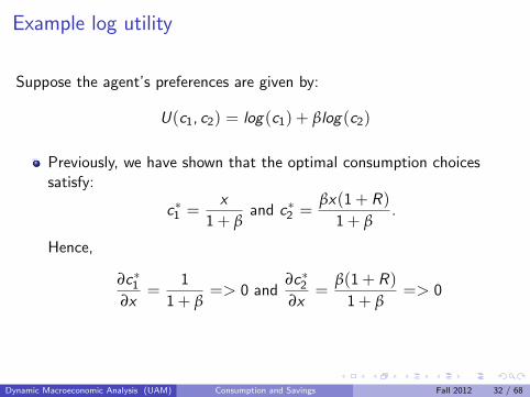
Example log utility
Suppose the agent’s preferences are given by:
U(c1, c2) = log(c1) + βlog(c2)
Previously, we have shown that the optimal consumption choicessatisfy:
c∗1 =x
1 + βand c∗2 =
βx(1 + R)1 + β
.
Hence,
∂c∗1∂x
=1
1 + β=> 0 and
∂c∗2∂x
=β(1 + R)
1 + β=> 0
Dynamic Macroeconomic Analysis (UAM) Consumption and Savings Fall 2012 32 / 68
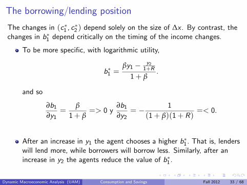
The borrowing/lending position
The changes in (c∗1 , c∗2 ) depend solely on the size of ∆x . By contrast, thechanges in b∗1 depend critically on the timing of the income changes.
To be more specific, with logarithmic utility,
b∗1 =βy1 − y2
1+R
1 + β.
and so
∂b1
∂y1=
β
1 + β=> 0 y
∂b1
∂y2= − 1
(1 + β)(1 + R)=< 0.
After an increase in y1 the agent chooses a higher b∗1 . That is, lenderswill lend more, while borrowers will borrow less. Similarly, after anincrease in y2 the agents reduce the value of b∗1 .
Dynamic Macroeconomic Analysis (UAM) Consumption and Savings Fall 2012 33 / 68
Interest rate changes
An increase in the interest rate provokes both an income and asubstitution effect:
substitution effect: The higher interest rate lowers the cost ofconsumption in the second period and makes saving more attractive.
Income effect: For given values of b1, the rise in R reduces thefeasible consumption levels for borrowers while it raises the wealth oflenders. The former need to pay higher interest payments, while thelatter receive higher interest payments.
Dynamic Macroeconomic Analysis (UAM) Consumption and Savings Fall 2012 34 / 68
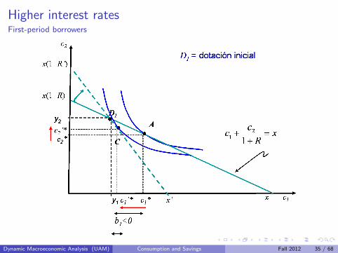
Higher interest ratesFirst-period borrowers
Dynamic Macroeconomic Analysis (UAM) Consumption and Savings Fall 2012 35 / 68
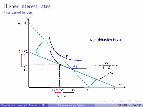
Higher interest ratesFirst-period lenders
Dynamic Macroeconomic Analysis (UAM) Consumption and Savings Fall 2012 36 / 68
The sum of income and substitution effectsThe combined effect of a higher interest rate on the consumption levelsdepends on the sign of b1.
First-period lenders (b∗1 > 0)Income effect: ∆c∗1 > 0 & ∆c∗2 > 0
Subst. effect: ∆c∗1 < 0 & ∆c∗2 > 0
Combined effect: ∆c∗1 ≷ 0 & ∆c∗2 > 0
∆c∗1 > 0 if the income effect dominates the substitution effect.
First-period borrowers (b∗1 < 0) :
Income effect: ∆c∗1 < 0 & ∆c∗2 < 0
Subst. effect: ∆c∗1 < 0 & ∆c∗2 > 0
Combined effect: ∆c∗1 < 0 & ∆c∗2 ≷ 0
∆c∗2 < 0 if income effect dominates the substitution effect.
Dynamic Macroeconomic Analysis (UAM) Consumption and Savings Fall 2012 37 / 68
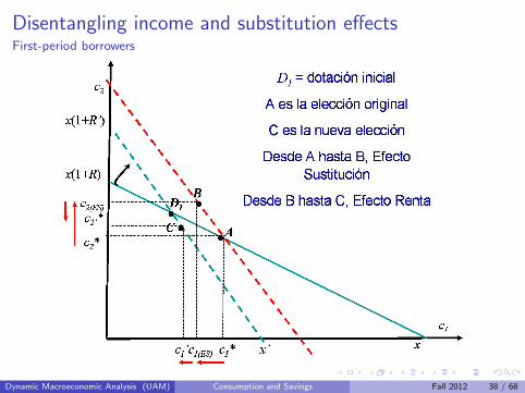
Disentangling income and substitution effectsFirst-period borrowers
Dynamic Macroeconomic Analysis (UAM) Consumption and Savings Fall 2012 38 / 68
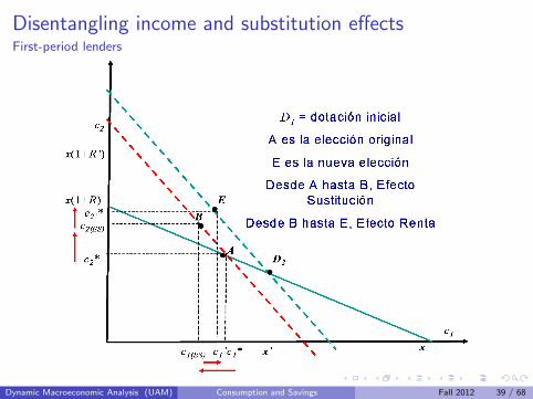
Disentangling income and substitution effectsFirst-period lenders
Dynamic Macroeconomic Analysis (UAM) Consumption and Savings Fall 2012 39 / 68
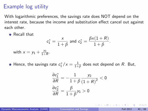
Example log utility
With logarithmic preferences, the savings rate does NOT depend on theinterest rate, because the income and substitution effect cancel out againsteach other.
Recall that
c∗1 =x
1 + βand c∗2 =
βx(1 + R)1 + β
.
with x = y1 + y21+R .
Hence, the savings rate c∗1 /x = 11+β does not depend on R. But,
∂c∗1∂R
= − 1
1 + β
y2
(1 + R)2< 0
∂c∗2∂R
=β
1 + βy1 > 0
Dynamic Macroeconomic Analysis (UAM) Consumption and Savings Fall 2012 40 / 68

Exercise II
Agents A and B have identical preferences over current and futureconsumption:
Ui = ln(c1,i ) + ln(c2,i ) con i = A, B
but they have different endowment patterns as (y1,A, y2,A) = (1, 0) y(y1,B , y2,B) = (0, 1), respectively.
a. Derive the solution for c∗1,i and c∗2,i and calculate the exact values ofthese variables for the case in which R = 0.
b. Analyze the effects of an increase in R.
c. Who benefits from the higher interest rate?
Dynamic Macroeconomic Analysis (UAM) Consumption and Savings Fall 2012 41 / 68
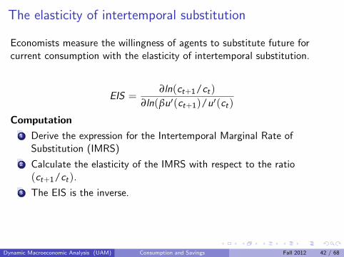
The elasticity of intertemporal substitution
Economists measure the willingness of agents to substitute future forcurrent consumption with the elasticity of intertemporal substitution.
EIS =∂ln(ct+1/ct)
∂ln(βu′(ct+1)/u′(ct)
Computation
1 Derive the expression for the Intertemporal Marginal Rate ofSubstitution (IMRS)
2 Calculate the elasticity of the IMRS with respect to the ratio(ct+1/ct).
3 The EIS is the inverse.
The EIS is important because it measures the elasticity of the optimalconsumption path to changes in the interest rate.
Dynamic Macroeconomic Analysis (UAM) Consumption and Savings Fall 2012 42 / 68
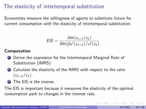

Example: Log Utility
For the case of logarithmic preferences U = log(c1) + βlog(c2) we have:
IMRS =dc2
dc1= − c2
βc1
The elasticity of the IMRS w.r.t. c2/c1 is given by
∂(− c2
βc1
)∂( c2
c1)∗
(c2c1
)(− c2
βc1
) = − 1
β∗ (−β) = 1
The EIS is the inverse of this number and so is 1.
Dynamic Macroeconomic Analysis (UAM) Consumption and Savings Fall 2012 43 / 68
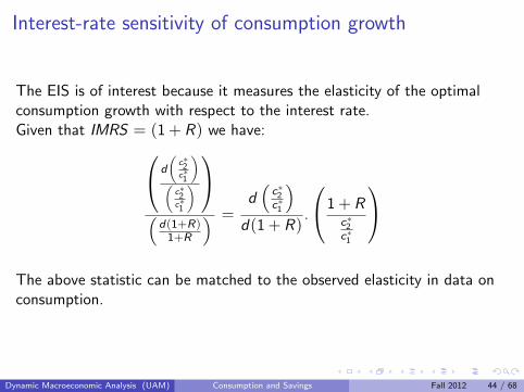
Interest-rate sensitivity of consumption growth
The EIS is of interest because it measures the elasticity of the optimalconsumption growth with respect to the interest rate.Given that IMRS = (1 + R) we have: d
(c∗2c∗1
)(
c∗2c∗1
)
(d(1+R)
1+R
) =d(
c∗2c∗1
)d(1 + R)
.
1 + Rc∗2c∗1
The above statistic can be matched to the observed elasticity in data onconsumption.
Dynamic Macroeconomic Analysis (UAM) Consumption and Savings Fall 2012 44 / 68
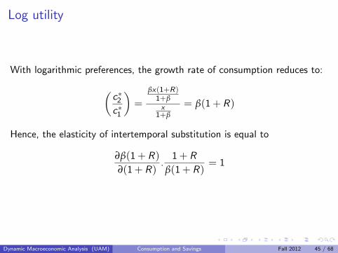
Log utility
With logarithmic preferences, the growth rate of consumption reduces to:
(c∗2c∗1
)=
βx(1+R)1+βx
1+β
= β(1 + R)
Hence, the elasticity of intertemporal substitution is equal to
∂β(1 + R)∂(1 + R)
.1 + R
β(1 + R)= 1
Dynamic Macroeconomic Analysis (UAM) Consumption and Savings Fall 2012 45 / 68
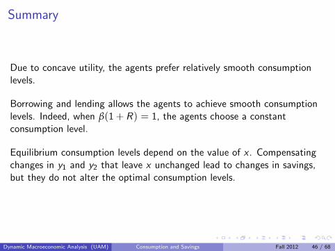
Summary
Due to concave utility, the agents prefer relatively smooth consumptionlevels.
Borrowing and lending allows the agents to achieve smooth consumptionlevels. Indeed, when β(1 + R) = 1, the agents choose a constantconsumption level.
Equilibrium consumption levels depend on the value of x . Compensatingchanges in y1 and y2 that leave x unchanged lead to changes in savings,but they do not alter the optimal consumption levels.
Dynamic Macroeconomic Analysis (UAM) Consumption and Savings Fall 2012 46 / 68
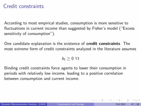
Credit constraints
According to most empirical studies, consumption is more sensitive tofluctuations in current income than suggested by Fisher’s model (“Excesssensitivity of consumption”).
One candidate explanation is the existence of credit constraints. Themost extreme form of credit constraints analyzed in the literature assumes
bt ≥ 0 ∀t
Binding credit constraints force agents to lower their consumption inperiods with relatively low income, leading to a positive correlationbetween consumption and current income.
Dynamic Macroeconomic Analysis (UAM) Consumption and Savings Fall 2012 47 / 68
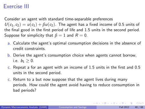
Exercise III
Consider an agent with standard time-separable preferencesU(c1, c2) = u(c1) + βu(c2). The agent has a fixed income of 0.5 units ofthe final good in the first period of life and 1.5 units in the second period.Suppose for simplicity that β = 1 and R = 0.
a. Calculate the agent’s optimal consumption decisions in the absence ofcredit constraints.
b. Derive the agent’s consumption choice when agents cannot borrow,i.e. b1 ≥ 0.
c. Repeat a for an agent with an income of 1.5 units in the first and 0.5units in the second period.
c. Return to a but now suppose that the agent lives during manyperiods. How could the agent avoid having to reduce consumption inbad periods?
Dynamic Macroeconomic Analysis (UAM) Consumption and Savings Fall 2012 48 / 68

N periods / Uncertainty
In real life, agents live for many agents and future income is uncertain. Inthese circumstances, agents need to solve
max{ct ,bt}
E0
N
∑t=0
βtu(ct)
subject to:ct + bt = yt + (1 + Rt)bt−1
Let λt denote the Lagrange multiplier associated with the period-t budgetconstraint. Case I: Without uncertainty and with Rt = R, the FOCs:
βtu′(ct) = λt
0 = −λt + (1 + R)λt+1 =⇒u′(ct) = β(1 + Rt)u′(ct+1)
Dynamic Macroeconomic Analysis (UAM) Consumption and Savings Fall 2012 49 / 68

Generalizing lifetime budget constraints
Consider the following sequence of budget constraints
c0 + b0 = y0
c1 + b1 = y1 + (1 + R)b0
.
.
cN + bN = yN + (1 + R)bN−1
Solving forwards, we obtain:
bN =N
∑t=0
yt
(1 + R)t−
N
∑t=0
ct
(1 + R)t
When life ends in N, bN = 0 and we obtain the standard expression.
Dynamic Macroeconomic Analysis (UAM) Consumption and Savings Fall 2012 50 / 68
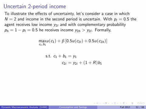
Uncertain 2-period incomeTo illustrate the effects of uncertainty, let’s consider a case in whichN = 2 and income in the second period is uncertain. With pl = 0.5 theagent receives low income y2l and with complementary probabilityph = 1− pl = 0.5 he receives income y2h > y2l . Formally,
maxc1,b1
u(c1) + β [0.5u(c2l ) + 0.5u(c2h)]
s.t. c1 + b1 = y1
c2i = y2i + (1 + R)b1
F.O.C:
u′(c1) = β(1 + R)[0.5u′(c2l ) + 0.5u′(c2h)]= β(1 + R)E1u′(y2i + (1 + R)b1)< β(1 + R)u′(E (y2i + (1 + R)b1))
Dynamic Macroeconomic Analysis (UAM) Consumption and Savings Fall 2012 51 / 68
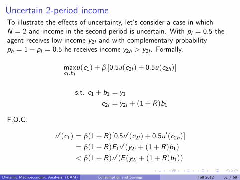
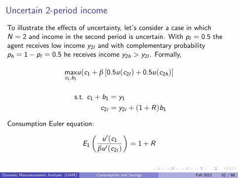
Uncertain 2-period income
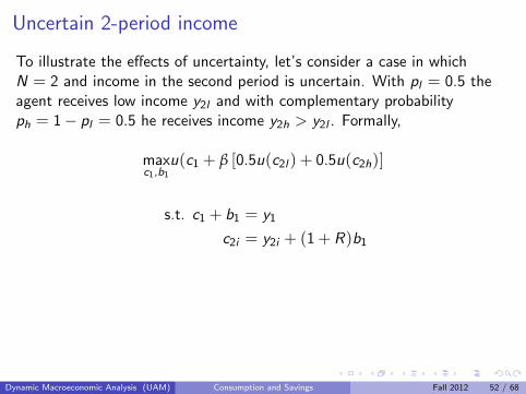
To illustrate the effects of uncertainty, let’s consider a case in whichN = 2 and income in the second period is uncertain. With pl = 0.5 theagent receives low income y2l and with complementary probabilityph = 1− pl = 0.5 he receives income y2h > y2l . Formally,
maxc1,b1
u(c1 + β [0.5u(c2l ) + 0.5u(c2h)]
s.t. c1 + b1 = y1
c2i = y2i + (1 + R)b1
Consumption Euler equation:
E1
(u′(c1
βu′(c2i )
)= 1 + R
Dynamic Macroeconomic Analysis (UAM) Consumption and Savings Fall 2012 52 / 68
Uncertain 2-period income
To illustrate the effects of uncertainty, let’s consider a case in whichN = 2 and income in the second period is uncertain. With pl = 0.5 theagent receives low income y2l and with complementary probabilityph = 1− pl = 0.5 he receives income y2h > y2l . Formally,
maxc1,b1
u(c1 + β [0.5u(c2l ) + 0.5u(c2h)]
s.t. c1 + b1 = y1
c2i = y2i + (1 + R)b1
Consumption Euler equation:
E1
(u′(c1
βu′(c2i )
)= 1 + R
Dynamic Macroeconomic Analysis (UAM) Consumption and Savings Fall 2012 52 / 68

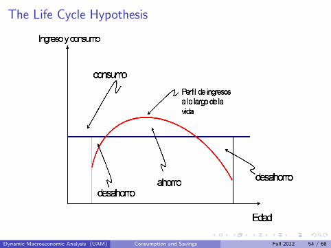
Life Cycle Hypothesis
Nobel prize winner Franco Modigliani considered an extension of thebasic model of Fisher to analyze decisions along the life cycle.
The basic insight: income varies in an almost deterministic manneralong the life cycle and agents use the credit market to insulateconsumption from these movements in income.
Agents typically borrow when they are young (education, housing),save during prime age and dissave during retirement.
At different stages of their life, agents or households therefore act atdifferent sides of the credit market.
Dynamic Macroeconomic Analysis (UAM) Consumption and Savings Fall 2012 53 / 68
The Life Cycle Hypothesis
Dynamic Macroeconomic Analysis (UAM) Consumption and Savings Fall 2012 54 / 68
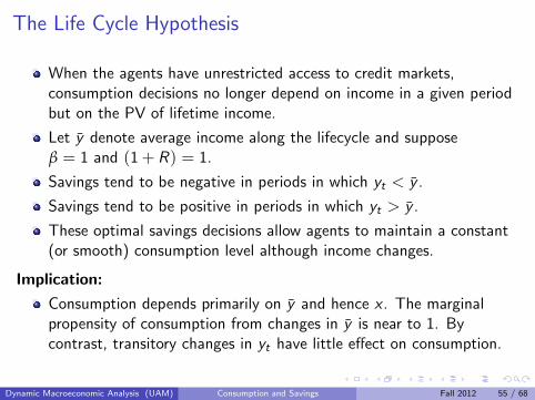
The Life Cycle Hypothesis
When the agents have unrestricted access to credit markets,consumption decisions no longer depend on income in a given periodbut on the PV of lifetime income.
Let y denote average income along the lifecycle and supposeβ = 1 and (1 + R) = 1.
Savings tend to be negative in periods in which yt < y .
Savings tend to be positive in periods in which yt > y .
These optimal savings decisions allow agents to maintain a constant(or smooth) consumption level although income changes.
Implication:
Consumption depends primarily on y and hence x . The marginalpropensity of consumption from changes in y is near to 1. Bycontrast, transitory changes in yt have little effect on consumption.
Dynamic Macroeconomic Analysis (UAM) Consumption and Savings Fall 2012 55 / 68
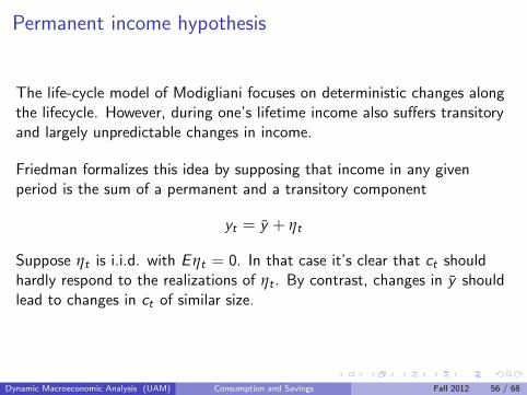
Permanent income hypothesis
The life-cycle model of Modigliani focuses on deterministic changes alongthe lifecycle. However, during one’s lifetime income also suffers transitoryand largely unpredictable changes in income.
Friedman formalizes this idea by supposing that income in any givenperiod is the sum of a permanent and a transitory component
yt = y + ηt
Suppose ηt is i.i.d. with E ηt = 0. In that case it’s clear that ct shouldhardly respond to the realizations of ηt . By contrast, changes in y shouldlead to changes in ct of similar size.
Dynamic Macroeconomic Analysis (UAM) Consumption and Savings Fall 2012 56 / 68
Random Walk Hypothesis
Bob Hall reconsidered the results of the permanent income hypothesis(PIH) assuming that agents have rational expectations — agents makeefficient use of all the available information.
Main prediction: If the PIH holds and agents have rational expectationsthen consumption changes should be unpredictable. That is, consumptionfollows a random walk and Etct+1 = ct .
In ordinary words: Agents only revise their consumption decisions if theyreceive new information that forces them to revise their expectations. Thisis intrinsically unpredictable.
Dynamic Macroeconomic Analysis (UAM) Consumption and Savings Fall 2012 57 / 68
Ejercicio III
Lucas vive durante dos periodos y su renta disponible en ambos periodoses y1 − τ1 y y2 − τ2, donde τt es un impuesto de cuantia fija en el perıodot. Suponga que Lucas tiene las siguientes preferencias:
U(c1, c2) = log(c1) + log(c2)
Suponga que el gobierno reduce el valor de τ1 en 1 unidad pero al mismomomento aumenta el impuesto en el segundo perıodo con (1 + R)unidades.
a. Analice como afectan los cambios en los impuestos al valor actual delos recursos totales de Lucas.
b. ¿Como afectan los cambias a las decisiones de consumo y ahorro deLucas?
Dynamic Macroeconomic Analysis (UAM) Consumption and Savings Fall 2012 58 / 68

Equilibrium with Many Agents
To end this second theme, we now proceed with an analysis of equilibriumconsumption and savings decisions in an economy with many agents.
Here we analyze the case of heterogenous agents with differentdegrees of impatience;
In the exercises we’ll consider the alternative case in which agentshave identical preferences but different income sequences.
In the latter case we are able to generate competitive equilibria in whichall agents end up with a constant consumption level during their lifetime.
Dynamic Macroeconomic Analysis (UAM) Consumption and Savings Fall 2012 59 / 68
Setup
Suppose the economy is populated by a large number of agents. Allagents have a constant income stream y1 = y2 = y . Hence,
x = y +y
1 + R.
There are two types of agents with different preferences. Ni agents oftype i with preferences
log(c1) + βi log(c2),
and Nj agents of type j with preferences
log(c1) + βj log(c2),
where βi < βj . In other words, the type-i agents are less patient thattheir type-j counterparts.
Dynamic Macroeconomic Analysis (UAM) Consumption and Savings Fall 2012 60 / 68
Individual problemRecall that the individual optimization problem of type-i agents can bewritten as:
maxc i
1
[u(c i1) + βiu((x − c i
1)(1 + R))]
Similarly, the Consumption Euler eqn. is:
c i2 = c i
1βi (1 + R).
Solutions:
c i1 =
x
1 + βi
c i2 =
β(1 + R)x
1 + βi
bi1 = y − c i
1 = y − x
1 + βi
=βiy − y
1+R
1 + βi.
Dynamic Macroeconomic Analysis (UAM) Consumption and Savings Fall 2012 61 / 68

Credit Market Equilibrium
In any equilibrium, the interest rate adjusts to ensure that the creditmarket clears. Formally,
Nibi1 + Njb
j1 = 0
Or equivalently,−Nib
i1︸ ︷︷ ︸
Creditdemand
= Njbj1︸︷︷︸
Creditsupply
Substituting the solutions for bi1 and bj
1 in the market clearing conditionyields:
Ni
βiy − y1+R
1 + βi+ Nj
βjy − y1+R
1 + βj= 0
Given the values for (y , βi , βj , Ni , Nj ) this equation can be solved for R.
Dynamic Macroeconomic Analysis (UAM) Consumption and Savings Fall 2012 62 / 68
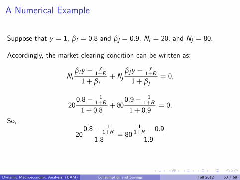
A Numerical Example
Suppose that y = 1, βi = 0.8 and βj = 0.9, Ni = 20, and Nj = 80.
Accordingly, the market clearing condition can be written as:
Ni
βiy − y1+R
1 + βi+ Nj
βjy − y1+R
1 + βj= 0,
200.8− 1
1+R
1 + 0.8+ 80
0.9− 11+R
1 + 0.9= 0,
So,
200.8− 1
1+R
1.8= 80
11+R − 0.9
1.9
Dynamic Macroeconomic Analysis (UAM) Consumption and Savings Fall 2012 63 / 68

Solution
200.8− 1
1+R
1.8= 80
11+R − 0.9
1.9
(0.8)20(1.9)− 1.9(20)1 + R
=80(1.8)1 + R
− (80)0.9(1.8),
30.4− 38
1 + R=
144
1 + R− 129.6.
30.4 + 129.6 =144
1 + R+
38
1 + R
160 =182
1 + R=⇒ 1 + R =
182
160=⇒ 1 + R = 1.1375
Dynamic Macroeconomic Analysis (UAM) Consumption and Savings Fall 2012 64 / 68
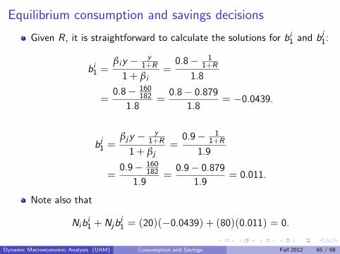
Equilibrium consumption and savings decisions
Given R, it is straightforward to calculate the solutions for bi1 and bj
1:
bi1 =
βiy − y1+R
1 + βi=
0.8− 11+R
1.8
=0.8− 160
182
1.8=
0.8− 0.879
1.8= −0.0439.
bj1 =
βjy − y1+R
1 + βj=
0.9− 11+R
1.9
=0.9− 160
182
1.9=
0.9− 0.879
1.9= 0.011.
Note also that
Nibi1 + Njb
j1 = (20)(−0.0439) + (80)(0.011) = 0.
Dynamic Macroeconomic Analysis (UAM) Consumption and Savings Fall 2012 65 / 68
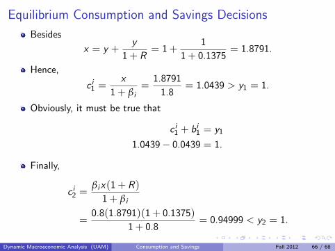
Equilibrium Consumption and Savings Decisions
Besides
x = y +y
1 + R= 1 +
1
1 + 0.1375= 1.8791.
Hence,
c i1 =
x
1 + βi=
1.8791
1.8= 1.0439 > y1 = 1.
Obviously, it must be true that
c i1 + bi
1 = y1
1.0439− 0.0439 = 1.
Finally,
c i2 =
βix(1 + R)1 + βi
=0.8(1.8791)(1 + 0.1375)
1 + 0.8= 0.94999 < y2 = 1.
Dynamic Macroeconomic Analysis (UAM) Consumption and Savings Fall 2012 66 / 68
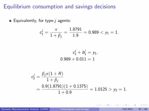
Equilibrium consumption and savings decisions
Equivalently, for type-j agents:
c j1 =
x
1 + βj=
1.8791
1.9= 0.989 < y1 = 1.
c j1 + bj
1 = y1,
0.989 + 0.011 = 1
c j2 =
βjx(1 + R)1 + βj
=0.9(1.8791)(1 + 0.1375)
1 + 0.9= 1.0125 > y2 = 1.
Dynamic Macroeconomic Analysis (UAM) Consumption and Savings Fall 2012 67 / 68

Summary
In this second part we have analyzed the competitive equilibrium inan economy of two periods;
All agents maximize their lifetime utility and can borrow or lend thedesired amount at the equilibrium interest rate;
All individuals enjoy a constant level of income. Nonetheless, inequilibrium
The impatient agents (type i) choose to borrow against their futureincome;
The impatient agents (type j) choose to lend part of their first-periodresources;
In the exercises you are invited to solve an example in which agentsuse the credit market to smooth their consumption;
Dynamic Macroeconomic Analysis (UAM) Consumption and Savings Fall 2012 68 / 68