Fiscal Policy, Consumption Home Bias and … of Applied Economics and Business Research JAEBR, 6(3): 194-217 (2016) Fiscal Policy, Consumption Home Bias and Macroeconomic Dynamics

Journal of Applied Economics and Business Research JAEBR, 6(3): 194-217 (2016)

Fiscal Policy, Consumption Home Bias and Macroeconomic

Dynamics

Chung-Fu Lai1 Fo Guang University, Taiwan, R.O.C Abstract In this paper we explore the dynamic adjustment process of fiscal expenditures shock on macroeconomic variables

(such as: consumption, output, prices, exchange rates, terms of trade) and the role of consumption home bias. A

New Open Economy Macroeconomics model with an imperfect competition setting and micro-foundation is used

as the analytical framework. Through theoretical derivations and simulation analysis, we find that in the long run,

increased government spending will cause domestic output, price and the exchange rate to rise, but crowd out

domestic private consumption. The relationship between government spending and terms of trade are not clear

and depends on the asymmetric consumption bias in two countries. In the short run, on the assumption that

consumers of both countries have a bias in favor of consuming home-produced goods, the volatility in domestic

consumption and output over the short run will be greater than that over the long run, thereby generating an

phenomenon of overshooting. Without the above assumption, the volatility in domestic consumption and output

over the short run will be smaller than that over the long run showing a undershooting phenomenon. In addition,

fiscal expenditure will not affect price, exchange rates and terms of trade, and the relationship between interest

rate and the government spending will be subject to asymmetric consumption bias.

Keywords: Fiscal policy, Consumption home bias, New Open Economy Macroeconomics

JEL Codes: E62, F41

Copyright © 2016 JAEBR

1. Introduction In the traditional Keynesian view, fiscal policy is an effective means to counter business cycle. In fact, when governmental role in economic regulation is highlighted, the operation of fiscal policy is also very positive. Various schools of thoughts have quite divided opinions about the

1 Correspondence to Chung-Fu Lai, E-mail: [email protected].

Copyright © 2016 JAEBR ISSN 1927-033X

mailto:[email protected]

Fiscal Policy, Consumption Home Bias and Macroeconomic Dynamics


195

effects of fiscal policy on output, consumption, interest rates and price.

In terms of public spending, Keynesian thought believes increased government spending will increase output and private investment, on the other hand, increased prices and interest rates will crowd out private sector investment which results in uncertain effects of private-sector investment. As for consumption of private sector, effects depend on size of the marginal propensity to consume and reaction to interest rate. The classical school believes fiscal policy only affects nominal variables and does not affect real variables. An Increase in government spending only cause price to rise. In addition, Neoclassical school emphasizes that temporary and permanent government spending have different effects on the macro economy. In addition, Supply-side economics prefer tax-cutting policy and believe it an incentive to increased amount of labor, increasing saving and investment, and can directly stimulate aggregate supply to increase reducing inflation and unemployment. The macroeconomic effects of fiscal policy on economic variables show great differences whether theoretical or empirical side. Besides, exchange rate is the relative price of domestic and foreign currencies which is charged with the important task of connecting domestic and international economics, regulating internal and external balance of the economy. Therefore, this paper explores effects of fiscal policy in a floating exchange rate system.

The initial development of analysis of open economy is Mundell-Fleming model (see Mundell, 1963; Fleming, 1962) and Dornbusch (1976) model which are derived from Keynesian theories. Although these early open economy models reveal and explain some of relationships among major economic variables, there is a common defect that is they lack micro-foundation. Lucas (1976) thinks that changes in macroeconomics variables can affect individual decisions in microeconomics, thereby causing changes in relationships among macroeconomic variables, resulting in bias in macro economy if the analysis lacks micro-foundation. Therefore, the birth of New Open Economy Macroeconomics (hereinafter referred to as NOEM) further opens a new stage of development of open macroeconomics. NOEM is a new-generation research method pertinent to open economy macroeconomics proposed by Obstfeld and Rogoff (1995). It has characteristics of micro-foundation and monopolistic competition market structure and is very suitable for analyzing impacts of exogenous shocks on macro economy. Therefore, this paper uses NOEM as basis for analysis.

There are four sections in this paper. Besides the introduction, the other sections are as follows: Section 2 convers a theoretical model, Section 3 includes the simulation analysis for exploring dynamic effects of fiscal expenditure shocks on macroeconomic variables as well as the role of consumption home bias plays, and section 4 are conclusions and recommendations.

C.-F. Lai


196

2. Literature Review

Theoretical and empirical literatures have inconsistent conclusions about effects of fiscal policy on economic activities, especially government expenditure shock on macroeconomic variables (such as private consumption, private investment, real wages, and employment). In theoretical literature, Real Business Cycle model proposed by Baxter and King (1993) assumed that consumer decision-making is subject to intertemporal budget constraints. When there is increased government spending financed with a fixed tax (lump-sum taxes), the present value of after-tax income will be reduced, resulting in a negative wealth effect that reduces consumption, and at a given wage level, labor supply will increase. In equilibrium, the real wages fall, employment and output increase. If the effect of employment continues, marginal productivity of capital will rise, resulting in increased investment (see Galí et al., 2007). In contrast, for traditional IS-LM model, its consumption is a function of disposable income rather than of lifetime earnings. Therefore, an increase in government spending will cause consumption to increase, and in the assumption that the money supply is fixed, nominal interest rates in the short-term will rise and private investment fall.

Moreover, studies about macroeconomic effects of fiscal policy concentrate on a closed economy (e.g. Barro, 1981; 1990, Futagami et al. 1993, Devereux and Love, 1995, Greiner, 1998, Greiner and Hanusch, 1998, Dasgupta, 1999, and Xie et al. 1999, etc.). Analysis of effects of fiscal policy in an open economy is relatively lacking. Until recently, with the rapid rise of NOEM such as Corsetti and Pesenti (2001); Ganelli (2003) and Pitterle and Steffen (2004a; 2004b), the studies on effects of fiscal policy now extend to open economic system. However, in the traditional NOEM model, exchange rate fluctuation is mainly caused by private consumption behavior. Therefore, in this paper we are interested to find out what will happen if we assume government behavior is included in consumer behavior and consumption home bias exist in both private and government purchasing behavior? So the purpose of this paper is to investigate the relationships among fiscal expenditure, consumption home bias and macroeconomic variables. Tervala (2008) analyzed the effects of fiscal policy under NOEM architecture, and it proved that the effect of government expenditure shock on welfare depend on the marginal rate of substitution of private and government consumption. However the paper ignores recent hot discussions about consumption home bias.

Although Obstfeld and Rogoff (2000) regards “home bias in consumption puzzle” as one of the six puzzles in international economics,2 but under NOEM architecture, there is a lack of complete research on the role of asymmetry in consumption home bias and this paper seeks

2 The six puzzles proposed by Obstfeld and Rogoff (2000) are consumption home bias puzzle, home bias in equity portfolios puzzle, purchasing power parity puzzle, exchange rate disconnect puzzle, the high investment-saving correlation puzzle, and the low international consumption correlation puzzle.



197

a breakthrough. The so-called consumption home bias puzzle means consumers have a tendency to prefer domestic goods in the real world, but this phenomenon cannot be explained by researchers. Early studies of consumption home bias mostly concentrate on the causes of it such as trade costs (Obstfeld and Rogoff, 2000; Ried, 2009), country size and openness (Sutherland, 2005; De Paoli, 2009), non-traded goods (Stockman and Dellas, 1989; Pesenti and Van Wincoop, 2002) as well as trade in intermediate input factors (Hillberry and Hummels, 2002). More recent researches focus on effects of consumption home bias. For example, Pierdzioch (2004) analyzed the effects of monetary shock in different degree of consumption home bias and capital mobility. Hau (2002), Pitterle and Steffen (2004a; 2004b), Kollmann (2004), Sutherland (2005), Leith and Lewis (2006) and Cooke (2010) investigated the effect of consumption home bias on exchange rate fluctuations. De Paoli (2009) discusses consumption home bias and welfare effects of monetary policy. Noting further that the effects of consumption home bias on monetary policy is quite a hot topic recently. Studies include Faia and Monacelli (2006), Jondeau and Sahuc (2008), Galí and Monacelli (2008) and Wang (2010). Obviously, there is abundant research related to topics about consumption home bias, but still there is no literature that can clearly explain the role of consumption home bias on the effect of fiscal expenditure shock, thus inducing the motivation of this paper.

3. Theoretical model

3.1 Model Setting

This paper follows NOEM proposed by Obstfeld and Rogoff (1995) as a theoretical basis; the main assumptions are stated as follows:

(1). There are two countries in the world, “home country” and “foreign country”, all of the following foreign economic variables are marked as “*” for identification.

(2). World population is distributed in the interval [0,1], where individuals of home country are distributed between [0, n ) and foreign individuals are distributed between [ n ,1].

(3). Each individual is both consumer and producer, and he operates a monopoly competitor factory uses labor for production.

(4). Consumption home bias behavior exists in economic system and government spending is the only exogenous shock.

(5). The price featured with stickiness and is not adjustable in the short term, but can be freely adjusted in the long term steady state.

C.-F. Lai


198

3.1.1 Household

Assuming that all individuals have the same preferences, utility (U ) and consumption ( C ) and real money balances ( PM / ) are in positive proportional, and is inversely proportional to the output ( y ), wherein, the lifetime utility function of representative individual is set as follows:

∑∞

=

−

−

−

−

+=ts

ss

ss

tst zy

PM

CU 21

)(21

log κε

χβε

, 0>ε (1)

Where β is the discount factor ( 10 << β ), ε is the elasticity of marginal utility of real money balance,3 χ and κ represent the degree of significance of real money balances and output on the utility function, z refers to a particular product.

In Eq. (1), define the consumption index of representative consumer as the constant elasticity of substitution (CES) function:

11

1

,

11

0 ,

1

)()1()(−

−−

−+= ∫∫

δδ

δδ

δδδ

δ ααn tf

n

tht dzzcdzzcC , 1>δ (2)

Where )(zch is the consumption of domestic consumer for domestic specific products

z , )(zc f is the consumption of domestic consumer for foreign specific product z , α is a

consumption home bias parameter measuring domestic consumers’ preference on domestic products, and δ is the elasticity of substitution of goods between two countries.

We can deduce domestic price index ( P ) from the definition of consumption index (Eq. (2)) by the problem of expenditure minimization as follows:

δδδ

αα−−

−

−+= ∫∫

11

1 1,

1

0 , )()1()(n tf

n

tht dzzpdzzpP

(3)

Likewise, the foreign price index (*P ) is as follows:

3 The elasticity of marginal utility of real money balance (ε ) is defined as the response of the change in the marginal utility of real money balances under a change of real money balances.



199

δδδ

αα−−

−

+−= ∫∫

11

1 1*,

*1

0

*,

** )()()1(n tf

n

tht dzzpdzzpP

(4)

In above two equations, )(zph represents the price of home commodity z expressed

in domestic currency, )(zp f represents domestic currency price of foreign goods z , )(* zph

represents the foreign currency price of domestic goods z , )(* zp f represents foreign

currency price of foreign goods z , *α stands for foreign consumers’ preference on foreign

products.

For any kind of goods, the law of one price is held as follows:

)()( *,, zpEzp thtth = (5)

)()( *,, zpEzp tfttf = (6)

where E represents the exchange rate.

From Eqs. (2) and (3), we can deduce the consumption of domestic representative consumer for specific home/foreign commodities as follows:

CP

zpzc th

th

δα −

=

)()( ,

,

(7)

CP

zpzc tf

tf

δα −

−=

)()1()( ,

,

(8)

Likewise, the consumption that foreign representative consumer for domestic specific commodity and foreign specific commodities as follows:

**

*,

**

,

)()1()( C

Pzp

zc thth

δα

−

−=

(9)

**

*,

**

,

)()( C

Pzp

zc tftf

δα

−

=

(10)

C.-F. Lai


200

In both formulas as above, )(* zch is the consumption of foreign consumer for specific

domestic products z , )(* zc f is the consumption of foreign consumer for specific foreign

products z .

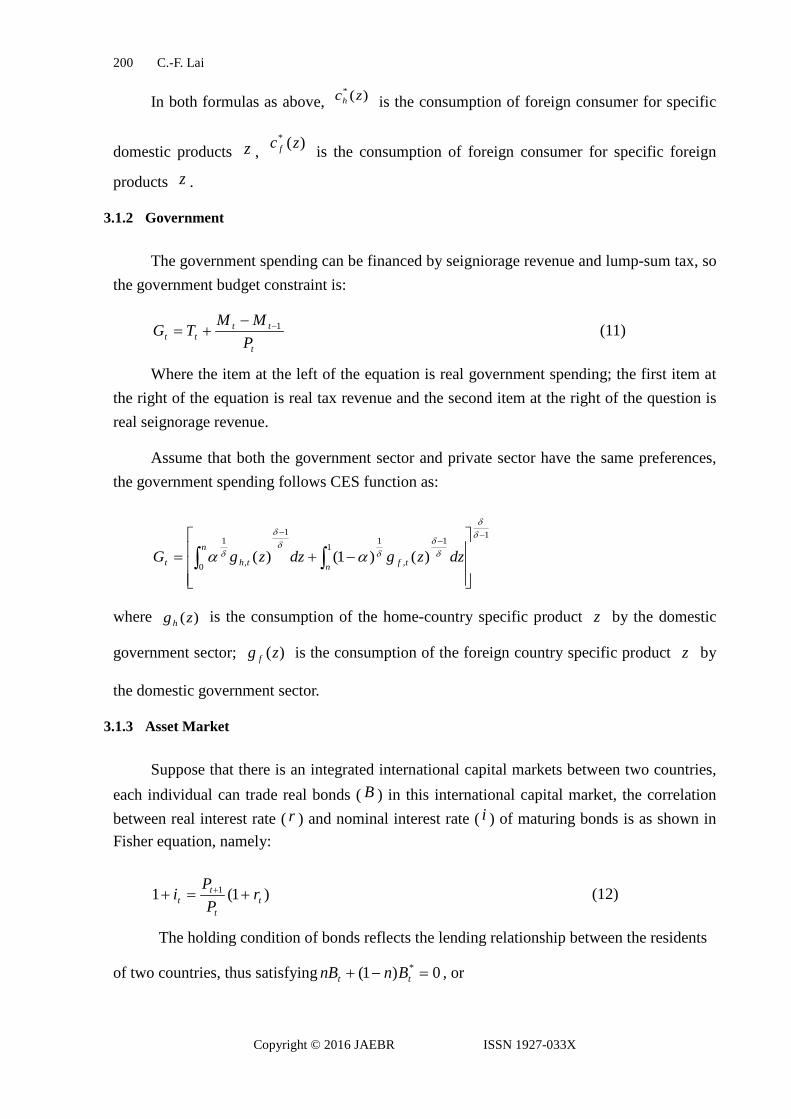
3.1.2 Government

The government spending can be financed by seigniorage revenue and lump-sum tax, so the government budget constraint is:

t

tttt P

MMTG 1−−+= (11)

Where the item at the left of the equation is real government spending; the first item at the right of the equation is real tax revenue and the second item at the right of the question is real seignorage revenue.

Assume that both the government sector and private sector have the same preferences, the government spending follows CES function as:

11

1

,

11

0 ,

1

)()1()(−

−−

−+= ∫∫

δδ

δδ

δδδ

δ ααn tf

n

tht dzzgdzzgG

where )(zgh is the consumption of the home-country specific product z by the domestic

government sector; )(zg f is the consumption of the foreign country specific product z by

the domestic government sector.

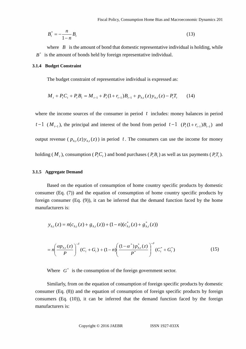
3.1.3 Asset Market

Suppose that there is an integrated international capital markets between two countries, each individual can trade real bonds ( B ) in this international capital market, the correlation between real interest rate ( r ) and nominal interest rate ( i ) of maturing bonds is as shown in Fisher equation, namely:

)1(1 1t

t

tt r

PP

i +=+ +

(12)

The holding condition of bonds reflects the lending relationship between the residents

of two countries, thus satisfying 0)1( * =−+ tt BnnB , or



201

tt Bn

nB−

−=1

*

(13)

where B is the amount of bond that domestic representative individual is holding, while *B is the amount of bonds held by foreign representative individual.

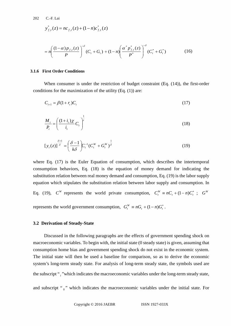
3.1.4 Budget Constraint

The budget constraint of representative individual is expressed as:

ttththttttttttt TPzyzpBrPMBPCPM −+++=++ −−− )()()1( ,,111 (14)

where the income sources of the consumer in period t includes: money balances in period

1−t ( 1−tM ), the principal and interest of the bond from period 1−t ))1(( 11 −−+ ttt BrP and

output revenue ( )()( ,, zyzp thth ) in period t . The consumers can use the income for money

holding ( tM ), consumption ( ttCP ) and bond purchases ( tt BP ) as well as tax payments ( ttTP ).

3.1.5 Aggregate Demand

Based on the equation of consumption of home country specific products by domestic consumer (Eq. (7)) and the equation of consumption of home country specific products by foreign consumer (Eq. (9)), it can be inferred that the demand function faced by the home manufacturers is:

))()()(1())()(()( *,

*,,,, zgzcnzgzcnzy ththththth +−++=

)()(,

ttth GC

Pzp

n +

=

−δα)(

)()1()1( **

*

*,

*

ttth GC

Pzp

n +

−−+

−δα (15)

Where *G is the consumption of the foreign government sector.

Similarly, from on the equation of consumption of foreign specific products by domestic consumer (Eq. (8)) and the equation of consumption of foreign specific products by foreign consumers (Eq. (10)), it can be inferred that the demand function faced by the foreign manufacturers is:

C.-F. Lai


202

)()1()()( *,,

*, zcnznczy tftftf −+=

)()()1( ,

tttf GC

Pzp

n +

−=

−δα)(

)()1( **

*

*,

*

tttf GC

Pzp

n +

−+

−δα

(16)

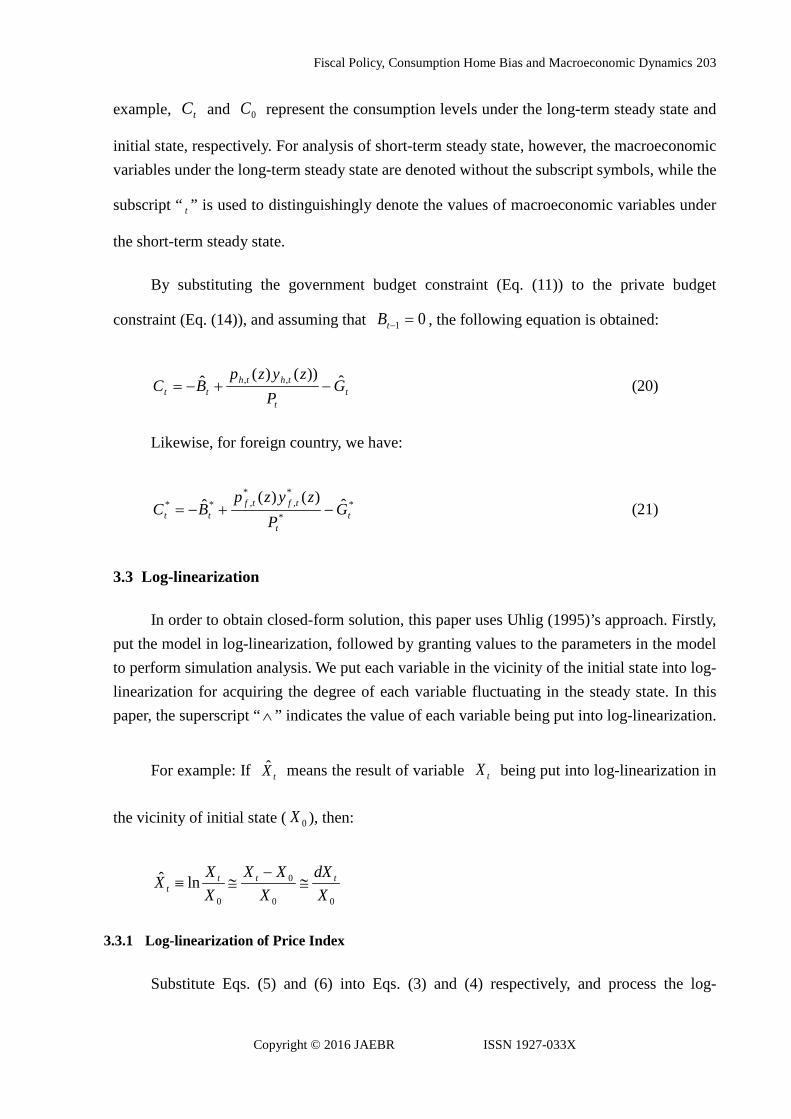
3.1.6 First Order Conditions

When consumer is under the restriction of budget constraint (Eq. (14)), the first-order conditions for the maximization of the utility (Eq. (1)) are:

ttt CrC )1(1 +=+ β (17)

εχ1

)1(

+= t

t

t

t

t Cii

PM

(18)

δδδ

δδ 1

11

)(1)]([ Wt

Wttt GCC

kzy +

−

= −+

(19)

where Eq. (17) is the Euler Equation of consumption, which describes the intertemporal consumption behaviors, Eq. (18) is the equation of money demand for indicating the substitution relation between real money demand and consumption, Eq. (19) is the labor supply equation which stipulates the substitution relation between labor supply and consumption. In

Eq. (19), WC represents the world private consumption, ∗−+≡ ttWt CnnCC )1( ; WG

represents the world government consumption, ∗−+≡ ttWt GnnGG )1( .

3.2 Derivation of Steady-State

Discussed in the following paragraphs are the effects of government spending shock on macroeconomic variables. To begin with, the initial state (0 steady state) is given, assuming that consumption home bias and government spending shock do not exist in the economic system. The initial state will then be used a baseline for comparison, so as to derive the economic system’s long-term steady state. For analysis of long-term steady state, the symbols used are

the subscript “ t ”which indicates the macroeconomic variables under the long-term steady state,

and subscript “ 0 ” which indicates the macroeconomic variables under the initial state. For



203

example, tC and 0C represent the consumption levels under the long-term steady state and

initial state, respectively. For analysis of short-term steady state, however, the macroeconomic variables under the long-term steady state are denoted without the subscript symbols, while the

subscript “ t ” is used to distinguishingly denote the values of macroeconomic variables under

the short-term steady state.

By substituting the government budget constraint (Eq. (11)) to the private budget

constraint (Eq. (14)), and assuming that 01 =−tB , the following equation is obtained:

tt

ththtt G

Pzyzp

BC ˆ))()(ˆ ,, −+−=

(20)

Likewise, for foreign country, we have:

**

*,

*,** ˆ)()(ˆ

tt

tftftt G

Pzyzp

BC −+−=

(21)

3.3 Log-linearization

In order to obtain closed-form solution, this paper uses Uhlig (1995)’s approach. Firstly, put the model in log-linearization, followed by granting values to the parameters in the model to perform simulation analysis. We put each variable in the vicinity of the initial state into log-linearization for acquiring the degree of each variable fluctuating in the steady state. In this paper, the superscript “∧ ” indicates the value of each variable being put into log-linearization.

For example: If tX means the result of variable tX being put into log-linearization in

the vicinity of initial state ( 0X ), then:

00

0

0

lnˆXdX

XXX

XXX ttt

t ≅−

≅≡

3.3.1 Log-linearization of Price Index

Substitute Eqs. (5) and (6) into Eqs. (3) and (4) respectively, and process the log-

C.-F. Lai


204

linearization to obtain:

))(ˆˆ)(1)(1()(ˆˆ *,, zpEnzpnP tfttht +−−+= αα (22)

)(ˆ)1()ˆ)(ˆ)(1(ˆ *,

*,

** zpnEzpnP tfttht αα −+−−= (23)

Subtract Eq. (23) from Eq. (22) to obtain the difference between fluctuations of price indices of two countries:

tthtt EnnzpnPP ˆ))1()1)(1(()())1((ˆˆ *,

** αααα −+−−+−−=−

)())1)((1( *,

* zpn tfαα −−−+ (24)

3.3.2 Log-linearization of the Law of One Price

Put Equation (5) and (6) into log-linearization to get:

)(ˆˆ)(ˆ *,, zpEzp thtth += (25)

)(ˆˆ)(ˆ *,, zpEzp tfttf += (26)

3.3.3 Log-linearization of World Budget Constraint

We may get the world budget constraints equation from Eqs. (20) and (21) as follows:

*)1( ttWt CnnCC −+=

+−=

t

ththt P

zyzpBn

)()( ,, Wt

t

tftft G

Pzyzp

Bn −

−−+ *

*,

*,* )()(ˆ)1(

(27)

Put Eq. (27) into log-linearization and use Eqs. (25) and (26) to get:

)ˆ)(ˆ)(ˆˆ(ˆ,, tththt

Wt PzyzpBnC −++−= W

tttftft GPzyzpBn ˆ)ˆ)(ˆ)(ˆ)(1( **,

*,

* −−++−−+ (28)

3.3.4 Log-linearization of Demand Function

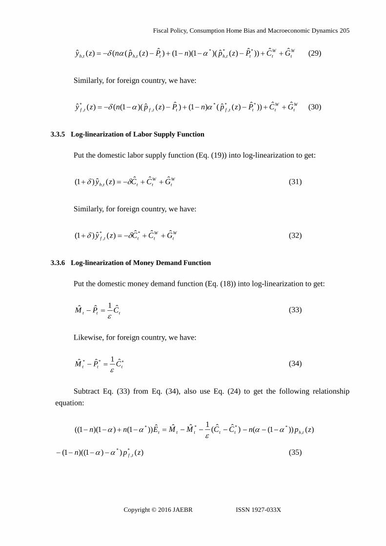
Put domestic and foreign demand functions (Eqs. (15) and (16)) into log-linearization to get:



205

Wt

Wttthtthth GCPzpnPzpnzy ˆˆ))ˆ)(ˆ)(1)(1()ˆ)(ˆ(()(ˆ **

,*

,, ++−−−+−−= ααδ (29)

Similarly, for foreign country, we have:

Wt

Wtttfttftf GCPzpnPzpnzy ˆˆ))ˆ)(ˆ()1()ˆ)(ˆ)(1(()(ˆ **

,*

,*

, ++−−+−−−= ααδ (30)

3.3.5 Log-linearization of Labor Supply Function

Put the domestic labor supply function (Eq. (19)) into log-linearization to get:

Wt

Wttth GCCzy ˆˆˆ)(ˆ)1( , ++−=+ δδ (31)

Similarly, for foreign country, we have:

Wt

Wtttf GCCzy ˆˆˆ)(ˆ)1( **

, ++−=+ δδ (32)

3.3.6 Log-linearization of Money Demand Function

Put the domestic money demand function (Eq. (18)) into log-linearization to get:

ttt CPM ˆ1ˆˆε

=−

(33)

Likewise, for foreign country, we have:

∗=− ttt CPM ˆ1ˆˆ **

ε (34)

Subtract Eq. (33) from Eq. (34), also use Eq. (24) to get the following relationship equation:

tEnn ˆ))1()1)(1(( *αα −+−− )ˆˆ(1ˆˆ **tttt CCMM −−−=

ε)())1(( ,

* zpn thαα −−−

)())1)((1( *,

* zpn tfαα −−−− (35)

C.-F. Lai


206

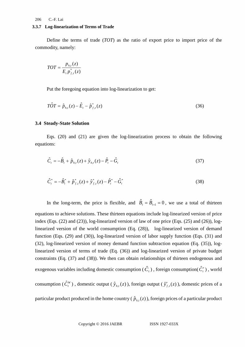
3.3.7 Log-linearization of Terms of Trade

Define the terms of trade (TOT) as the ratio of export price to import price of the commodity, namely:

)()(

*,

,

zpEzp

TOTtft

th=

Put the foregoing equation into log-linearization to get:

)(ˆˆ)(ˆˆ *,, zpEzpTOT tftth −−= (36)

3.4 Steady-State Solution

Eqs. (20) and (21) are given the log-linearization process to obtain the following equations:

ttththtt GPzyzpBC ˆˆ)(ˆ)(ˆˆˆ,, −−++−= (37)

***,

*,

** ˆˆ)(ˆ)(ˆˆˆtttftftt GPzyzpBC −−++−= (38)

In the long-term, the price is flexible, and 0ˆˆ1 == +tt BB , we use a total of thirteen

equations to achieve solutions. These thirteen equations include log-linearized version of price index (Eqs. (22) and (23)), log-linearized version of law of one price (Eqs. (25) and (26)), log-linearized version of the world consumption (Eq. (28)), log-linearized version of demand function (Eqs. (29) and (30)), log-linearized version of labor supply function (Eqs. (31) and (32), log-linearized version of money demand function subtraction equation (Eq. (35)), log-linearized version of terms of trade (Eq. (36)) and log-linearized version of private budget constraints (Eq. (37) and (38)). We then can obtain relationships of thirteen endogenous and

exogenous variables including domestic consumption ( tC ) , foreign consumption( ∗tC ) , world

consumption ( WtC ) , domestic output ( )(ˆ , zy th ), foreign output ( )(ˆ , zy tf

∗ ), domestic prices of a

particular product produced in the home country ( )(ˆ , zp th ), foreign prices of a particular product



207

produced in the home country ( )(ˆ *, zp th ), foreign price of a particular product produced in a

foreign country ( )(ˆ , zp tf∗ )), domestic price of a particular product produced in the foreign

country ( )(ˆ , zp tf )), exchange rate ( tE ), domestic price index ( tP ), foreign price index ( *tP ) as

well as the terms of trade ( tTOT ˆ ).

In the short-term, price is rigid ( 0)(ˆ , =zp th ； 0)(ˆ , =∗ zp tf ). Separately, with log-linearized

of consumption Euler equation (Eq. (17)) of the home country and Euler equation of foreign consumption, we can obtain the changes in world consumption of short-term as follows:

tWW

t rCC ˆ)1(ˆˆ β−−= (39)

We now can use a total of fourteen equations to achieve solutions in the short-term. These include log-linearized version of price index (Eqs. (22) and (23)), log -linearized version of law of one price (Eqs. (25) and (26)), log-linearized version of the world consumption (Eq. (28)), log-linearized version of demand function (Eqs. (29) and (30)), log-linearized version of labor supply function (Eqs. (31) and (32)), log-linearized version of money demand function subtraction formula (Eq. (35)), log-linearized version of terms of trade (Eq. (36)) and log-linearized version of private budget constraints (Eqs. (37) and (38)), and the equation of relationship of world consumption in the long-term and short-term equation (Eq. (39)). We then can obtain relationships of fourteen endogenous and exogenous variables ( G ) including

domestic consumption ( tC ) , foreign consumption( ∗tC ) , world consumption ( W

tC ) , domestic

output ( )(ˆ , zy th ), foreign output ( )(ˆ , zy tf∗ ), foreign prices of a particular product produced in the

home country ( )(ˆ *, zp th ), domestic price of a particular product produced in the foreign country

( )(ˆ , zp tf )), the exchange rate ( tE ), domestic price index ( tP ), foreign price index ( *tP ), the

domestic current account ( tB ), the foreign current account t( *ˆtB ) as well as the terms of trade

( tTOT ˆ ).

C.-F. Lai


208

4. The Effects of Government Spending Shocks on Macroeconomic Variables

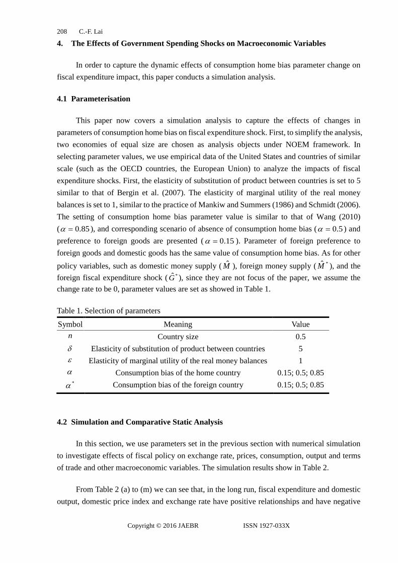
In order to capture the dynamic effects of consumption home bias parameter change on fiscal expenditure impact, this paper conducts a simulation analysis.

4.1 Parameterisation

This paper now covers a simulation analysis to capture the effects of changes in parameters of consumption home bias on fiscal expenditure shock. First, to simplify the analysis, two economies of equal size are chosen as analysis objects under NOEM framework. In selecting parameter values, we use empirical data of the United States and countries of similar scale (such as the OECD countries, the European Union) to analyze the impacts of fiscal expenditure shocks. First, the elasticity of substitution of product between countries is set to 5 similar to that of Bergin et al. (2007). The elasticity of marginal utility of the real money balances is set to 1, similar to the practice of Mankiw and Summers (1986) and Schmidt (2006). The setting of consumption home bias parameter value is similar to that of Wang (2010) ( 85.0=α ), and corresponding scenario of absence of consumption home bias ( 5.0=α ) and preference to foreign goods are presented ( 15.0=α ). Parameter of foreign preference to foreign goods and domestic goods has the same value of consumption home bias. As for other policy variables, such as domestic money supply ( M ), foreign money supply ( *M ), and the foreign fiscal expenditure shock ( *G ), since they are not focus of the paper, we assume the change rate to be 0, parameter values are set as showed in Table 1.

Table 1. Selection of parameters

Symbol Meaning Value n Country size 0.5 δ Elasticity of substitution of product between countries 5 ε Elasticity of marginal utility of the real money balances 1 α Consumption bias of the home country 0.15; 0.5; 0.85

*α Consumption bias of the foreign country 0.15; 0.5; 0.85

4.2 Simulation and Comparative Static Analysis

In this section, we use parameters set in the previous section with numerical simulation to investigate effects of fiscal policy on exchange rate, prices, consumption, output and terms of trade and other macroeconomic variables. The simulation results show in Table 2.

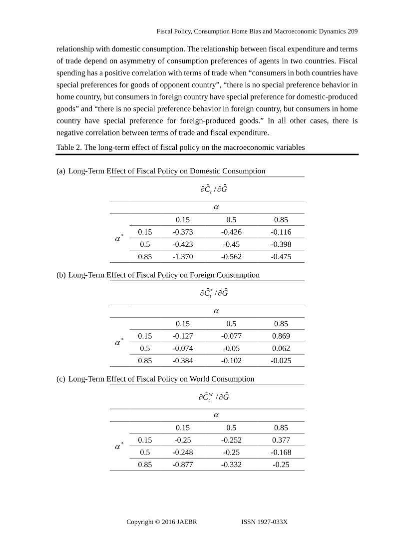
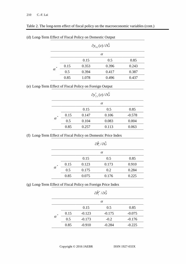
From Table 2 (a) to (m) we can see that, in the long run, fiscal expenditure and domestic output, domestic price index and exchange rate have positive relationships and have negative



209

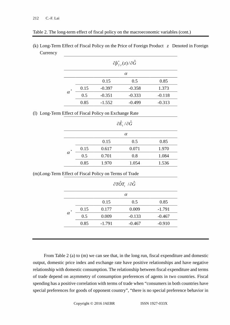
relationship with domestic consumption. The relationship between fiscal expenditure and terms of trade depend on asymmetry of consumption preferences of agents in two countries. Fiscal spending has a positive correlation with terms of trade when “consumers in both countries have special preferences for goods of opponent country”, “there is no special preference behavior in home country, but consumers in foreign country have special preference for domestic-produced goods” and “there is no special preference behavior in foreign country, but consumers in home country have special preference for foreign-produced goods.” In all other cases, there is negative correlation between terms of trade and fiscal expenditure.

Table 2. The long-term effect of fiscal policy on the macroeconomic variables

(a) Long-Term Effect of Fiscal Policy on Domestic Consumption

GCtˆ/ˆ ∂∂

α

*α

0.15 0.5 0.85 0.15 -0.373 -0.426 -0.116 0.5 -0.423 -0.45 -0.398 0.85 -1.370 -0.562 -0.475

(b) Long-Term Effect of Fiscal Policy on Foreign Consumption

GCtˆ/ˆ * ∂∂

α

*α

0.15 0.5 0.85 0.15 -0.127 -0.077 0.869 0.5 -0.074 -0.05 0.062 0.85 -0.384 -0.102 -0.025

(c) Long-Term Effect of Fiscal Policy on World Consumption

GCWt

ˆ/ˆ ∂∂

α

*α

0.15 0.5 0.85 0.15 -0.25 -0.252 0.377 0.5 -0.248 -0.25 -0.168 0.85 -0.877 -0.332 -0.25

C.-F. Lai


210

Table 2. The long-term effect of fiscal policy on the macroeconomic variables (cont.)

(d) Long-Term Effect of Fiscal Policy on Domestic Output

Gzy thˆ/)(, ∂∂

α

*α

0.15 0.5 0.85 0.15 0.353 0.396 0.243 0.5 0.394 0.417 0.387 0.85 1.078 0.496 0.437

(e) Long-Term Effect of Fiscal Policy on Foreign Output

Gzy tfˆ/)(*

, ∂∂

α

*α

0.15 0.5 0.85 0.15 0.147 0.106 -0.578 0.5 0.104 0.083 0.004 0.85 0.257 0.113 0.063

(f) Long-Term Effect of Fiscal Policy on Domestic Price Index

GPtˆ/ˆ ∂∂

α

*α

0.15 0.5 0.85 0.15 0.123 0.173 0.910 0.5 0.175 0.2 0.284 0.85 0.075 0.176 0.225

(g) Long-Term Effect of Fiscal Policy on Foreign Price Index

GPtˆ/ˆ * ∂∂

α

*α

0.15 0.5 0.85 0.15 -0.123 -0.175 -0.075 0.5 -0.173 -0.2 -0.176 0.85 -0.910 -0.284 -0.225



211


(h) Long-Term Effect of Fiscal Policy on the Price of Domestic Product z Denoted in Domestic Currency

Gzp thˆ/)(ˆ , ∂∂

α

*α

0.15 0.5 0.85 0.15 0.397 0.351 1.552 0.5 0.358 0.333 0.499 0.85 -1.373 0.118 0.313

(i) Long-Term Effect of Fiscal Policy on the Price of Domestic Product z Denoted in Foreign Currency

Gzp thˆ/)(ˆ *

, ∂∂

α

*α

0.15 0.5 0.85 0.15 -0.220 -0.350 -0.418 0.5 -0.342 -0.467 -0.585 0.85 -3.343 -0.966 -1.223

(j) Long-Term Effect of Fiscal Policy on the Price of Foreign Product z Denoted in Domestic Currency

Gzp tfˆ/)(ˆ , ∂∂

α

*α

0.15 0.5 0.85 0.15 0.220 0.342 3.343 0.5 0.350 -0.467 0.966 0.85 0.418 0.585 1.223

C.-F. Lai


212


(k) Long-Term Effect of Fiscal Policy on the Price of Foreign Product z Denoted in Foreign Currency

Gzp tfˆ/)(ˆ *

, ∂∂

α

*α

0.15 0.5 0.85 0.15 -0.397 -0.358 1.373 0.5 -0.351 -0.333 -0.118 0.85 -1.552 -0.499 -0.313

(l) Long-Term Effect of Fiscal Policy on Exchange Rate

GEtˆ/ˆ ∂∂

α

*α

0.15 0.5 0.85 0.15 0.617 0.071 1.970 0.5 0.701 0.8 1.084 0.85 1.970 1.054 1.536

(m) Long-Term Effect of Fiscal Policy on Terms of Trade

GTOT tˆ/ˆ ∂∂

α

*α

0.15 0.5 0.85 0.15 0.177 0.009 -1.791 0.5 0.009 -0.133 -0.467 0.85 -1.791 -0.467 -0.910

From Table 2 (a) to (m) we can see that, in the long run, fiscal expenditure and domestic output, domestic price index and exchange rate have positive relationships and have negative relationship with domestic consumption. The relationship between fiscal expenditure and terms of trade depend on asymmetry of consumption preferences of agents in two countries. Fiscal spending has a positive correlation with terms of trade when “consumers in both countries have special preferences for goods of opponent country”, “there is no special preference behavior in



213

home country, but consumers in foreign country have special preference for domestic-produced goods” and “there is no special preference behavior in foreign country, but consumers in home country have special preference for foreign-produced goods.” In all other cases, there is negative correlation between terms of trade and fiscal expenditure.

Economic intuitions behind these conclusions can be explained as follows: an increase in government spending increase demand for domestic goods, leading to increase domestic output and price. But because of the “crowding out effect”, there will be decline in private consumption and money demand, leading to depreciation of domestic currency (raise of exchange rate). As for the relationship between government spending and terms of trade, uncertainty arise because of mutual exclusive effects of increased prices and exchange rates, which is depend on asymmetry of consumption bias of agent in the two countries.

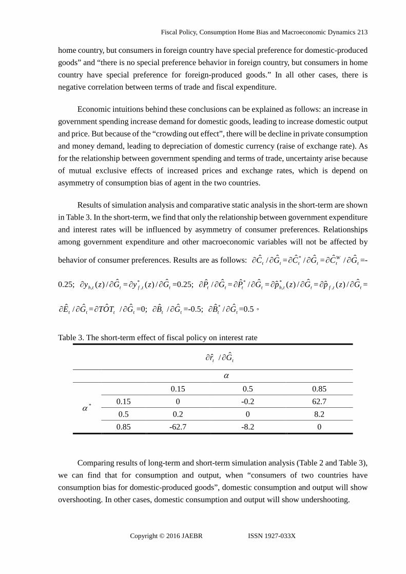
Results of simulation analysis and comparative static analysis in the short-term are shown in Table 3. In the short-term, we find that only the relationship between government expenditure and interest rates will be influenced by asymmetry of consumer preferences. Relationships among government expenditure and other macroeconomic variables will not be affected by

behavior of consumer preferences. Results are as follows: tt GC ˆ/ˆ ∂∂ = tt GC ˆ/ˆ * ∂∂ = tWt GC ˆ/ˆ ∂∂ =-

0.25; tth Gzy ˆ/)(, ∂∂ = ttf Gzy ˆ/)(*, ∂∂ =0.25; tt GP ˆ/ˆ ∂∂ = tt GP ˆ/ˆ * ∂∂ = tth Gzp ˆ/)(ˆ *

, ∂∂ = ttf Gzp ˆ/)(ˆ , ∂∂ =

tt GE ˆ/ˆ ∂∂ = tt GTOT ˆ/ˆ ∂∂ =0; tt GB ˆ/ˆ ∂∂ =-0.5; tt GB ˆ/ˆ * ∂∂ =0.5。

Table 3. The short-term effect of fiscal policy on interest rate

tt Gr ˆ/ˆ ∂∂

α

*α

0.15 0.5 0.85 0.15 0 -0.2 62.7 0.5 0.2 0 8.2 0.85 -62.7 -8.2 0

Comparing results of long-term and short-term simulation analysis (Table 2 and Table 3), we can find that for consumption and output, when “consumers of two countries have consumption bias for domestic-produced goods”, domestic consumption and output will show overshooting. In other cases, domestic consumption and output will show undershooting.

C.-F. Lai


214

As for short-term effects of fiscal expenditure on price, exchange rates and terms of trade, since the price is rigid, price, exchange rates and terms of trade are not affected by fiscal expenditure shock, relations between fiscal expenditure and interest rates will be subject to the asymmetry of consumption bias. In the cases of “domestic consumers have preferences for foreign goods, and foreign consumers do not have consumption bias”, “consumers of two countries prefer domestic-produced goods” and “domestic consumers prefer domestic products, and foreign consumers do not have consumption bias”, an increase in fiscal spending will result in decrease in public sector savings, monetary supply, leading to higher interest rates. In other cases of “consumers of two countries prefer foreign-produced products”, “domestic consumers have no consumption bias and foreign consumers prefer domestic-produced goods”, and “domestic consumers do not have consumption bias, and foreign consumers have preferences for foreign-produced goods”, an increase in fiscal spending will cause interest rates to fall.

5. Conclusion

It has been more than 20 years since the development of NOEM model. Compared to the popularity study of impacts of monetary policy, studies of the effects of fiscal policy are relatively lacking. Due to the above reason, this paper uses theoretical framework of NOEM proposed by Obstfeld and Rogoff (1995), integrated with consumption home bias to explore dynamic effects of macroeconomic variables when a country is faced with fiscal expenditure shocks. We hope results of this paper can be used as reference for policy-making by relevant authorities.

Through theoretical derivation and simulation results, we find out in the face of fiscal expenditure shock, except the case of “consumers of two countries have special preferences for domestically-produced goods,” fluctuations in domestic consumption and output in the short term will be bigger than those in the long term, showing an overshooting phenomenon. In other cases, fiscal expenditure shock does not affect price, exchange rates and terms of trade. Relationship between interest rate and fiscal expenditure shock will be subject to asymmetry of consumption bias, which can cause short-term interest rates to rise or fall.

Finally, one should notice that although NOEM framework plays an important role in various economic issues, many assumptions are required if one wants to easily achieve solutions. If one of the assumptions or settings no longer exists, the results may differ, we deem this deficiency as one of restrictions of this paper.

References

Barro, R. J. 1981. Output Effect of Government Purchases. Journal of Public Economy 89, 1086-1121.



215

Barro, R. J. 1990. Government Spending in a Simple Model of Endogenous Growth. Journal of Political Economy 98, S103-S125.

Baxter, M., and King R, G. 1993. Fiscal Policy in General Equilibrium. American Economic Review 83:3, 315-333.

Bergin, P. R., Shin, H. C., and Tchakarov, I. 2007. Does Exchange Rate Variability Matter for Welfare? A Quantitative Investigation of Stabilization Policies. European Economic Review 51:4, 1041-1058.

Cooke, D. 2010. Consumption Home Bias and Exchange Rate Behavior. Journal of Macroeconomics 32:1, 415-425.

Corsetti, G., and Pesenti, P. 2001. Welfare and Macroeconomic Interdependence. Quarterly Journal of Economics 116, 421-446.

Dasgupta, D. 1999. Growth versus Welfare in a Model of Nonrival Infrastructure. Journal of Development Economics 58, 359-385.

De Paoli, B. 2009. Monetary Policy and Welfare in a Small Open Economy. Journal of International Economics 77:1, 11-22.

Devereux M. B., and Love, D. R. F. 1995. The Dynamic Effects of Government Spending Policies in a Two-Sector Endogenous Growth Model. Journal of Money, Credit, and Banking 27, 232-256.

Dornbusch, R. 1976. Expectations and Exchange Rate Dynamics. Journal of Political Economy 84, 1161-1176.

Faia, E., and Monacelli, T. 2006. Optimal Monetary Policy in a Small Open Economy with Home Bias. CEPR Discussion Papers, No. 5522.

Fleming, J. M. 1962. Domestic Financial Policies Under Fixed and Under Floating Exchange Rates. IMF Staff Papers 9, 369-379.

Futagami, K., Morita, Y., and Shibata, A. 1993. Dynamic Analysis of an Endogenous Growth Model with Public Capital. Scandinavian Journal of Economics 95, 607-625.

Galí, J., and Monacelli, T. 2008. Optimal Monetary and Fiscal Policy in a Currency Union. Journal of International Economics 76:1, 116-132.

Galí, J., Lopez-Salido, D., and Valles, J. 2007. Understanding the Effects of Government Spending on Consumption. Journal of the European Economic Association 5:1, 227–270.

Ganelli, G. 2003. Useful Government Spending, Direct Crowding-out and Fiscal Policy Interdependence. Journal of International Money and Finance 22, 87-103.

Greiner, M. 1998. Fiscal Policy in an Endogenous-Growth Model with Public Investment: A Note. Journal of Economics 68, 193-198.

Greiner, M., and Hanusch, H. 1998. Growth and Welfare Effects of Fiscal Policy in an Endogenous Growth Model with Public Investment. International Tax and Public Finance 5, 249-261.

Hau, H. 2002. Real Exchange Rate Volatility and Economic Openness: Theory and Evidence.

C.-F. Lai


216

Journal of Money, Credit and Banking 34, 611-630. Hillberry, R. H., and Hummels, D. L. 2002. “Explaining Home Bias in Consumption: The Role

of Intermediate Input Trade,” NBER Working Paper, No. 9020. Jondeau, E., and Sahuc, J. G. 2008. Optimal Monetary Policy in an Estimated DSGE Model of

the Euro Area with Cross-Country Heterogeneity. International Journal of Central Banking 4, 23-72.

Kollmann, R. 2004. Welfare Effects of a Monetary Union: The Role of Trade Openness. Journal of the European Economic Association 2, 289-301.

Leith, C., and Lewis, S. W. 2006. The Optimal Monetary Policy Response to Exchange Rate Misalignment. Center for Dynamic Macroeconomic Analysis Conference Papers.

Lucas, R. E. 1976. Econometric Policy Evaluation: A Critique. Carnegie-Rochester Conference Series on Public Policy 1, 19-46.

Mankiw, N. G., and Summers, L. H. 1986. Money Demand and the Effects of Fiscal Policies. Journal of Money, Credit and Banking 18:4, 415-429.

Mundell, R. A. 1963. Capital Mobility and Stabilization Policy under Fixed and Flexible Exchange Rates. Canadian Journal of Economics and Political Science 29, 475-485.

Obstfeld, M., and Rogoff, K. 1995. Exchange Rate Dynamics Redux. Journal of Political Economy 103, 624-660.

Obstfeld, M., and Rogoff, K. 2000. The Six Major Puzzles in International Macroeconomics: Is There a Common Cause?. in B.S. Bernanke and K. Rogoff, eds., NBER Macroeconomics Annual 15, 339-390.

Pesenti, P., and Van Wincoop, E. 2002. Can Nontradables Generate Substantial Home Bias?. Journal of Money, Credit, and Banking 34:1, 25-50.

Pierdzioch, C. 2004. Home-Product Bias, Capital Mobility, and the Effects of Monetary Policy Shocks in Open Economies. Kiel Working Paper, No. 1141.

Pitterle, I., and Steffen, D. 2004a. Fiscal Policy in a Monetary Union Model with Home Bias in Consumption. Mimeo, University of Frankfurt.

Pitterle, I., and Steffen, D. 2004b. Spillover Effects of Fiscal Policy under Flexible Exchange Rate. Working Paper, University of Frankfurt.

Ried, S. 2009. Putting Up a Good Fight: The Galí-Monacelli Model versus “The Six Major Puzzles in International Macroeconomics”. SFB 649 Discussion Papers, Humboldt University, Berlin, Germany.

Schmidt, C. 2006. International Transmission Effects of Monetary Policy Shocks: Can Asymmetric Price Setting Explain the Stylized Facts?. International Journal of Finance and Economics 11, 205-218.

Stockman, A. C., and Dellas, H. 1989. International Portfolio Nondiversification and Exchange Rate Variability. Journal of International Economics 26, 271-289.

Sutherland, A. 2005. Incomplete Pass-Through and the Welfare Effects of Exchange Rate Variability. Journal of International Economics 65, 375-399.



217

Tervala, J. 2008. Productive Government Spending, Welfare and Exchange Rate Dynamics. Financial Theory and Practice 32, 97-114.

Uhlig, H. 1995. A Toolkit for Analyzing Nonlinear Dynamic Stochastic Models Easily. Center for Economic Research Discussion Paper, No. 97, Tilburg University.

Wang J. 2010. Home Bias, Exchange Rate Disconnect, and Optimal Exchange Rate Policy. Journal of International Money and Finance 29, 55-78.

Xie, D., Zou, H, F., and Davoodi, H. 1999. Fiscal Decentralization and Economic Growth in the United State. Journal of Urban Economics 45, 228-239.

Documents

Fiscal Policy, Consumption Home Bias and … of Applied Economics and Business Research JAEBR, 6(3): 194-217 (2016) Fiscal Policy, Consumption Home Bias and Macroeconomic Dynamics