Atmos. Meas. Tech., 11, 1937–1946, 2018https://doi.org/10.5194/amt-11-1937-2018© Author(s) 2018. This work is distributed underthe Creative Commons Attribution 4.0 License.

The BErkeley Atmospheric CO2 Observation Network: fieldcalibration and evaluation of low-cost air quality sensorsJinsol Kim1, Alexis A. Shusterman2, Kaitlyn J. Lieschke2, Catherine Newman2, and Ronald C. Cohen1,2

1Department of Earth and Planetary Science, University of California Berkeley, Berkeley, CA 94720, USA2Department of Chemistry, University of California Berkeley, Berkeley, CA 94720, USA

Correspondence: Ronald C. Cohen (rccohen@berkeley.edu)

Received: 18 September 2017 – Discussion started: 28 September 2017Revised: 8 February 2018 – Accepted: 3 March 2018 – Published: 6 April 2018

Abstract. The newest generation of air quality sensors issmall, low cost, and easy to deploy. These sensors are an at-tractive option for developing dense observation networks insupport of regulatory activities and scientific research. Theyare also of interest for use by individuals to characterizetheir home environment and for citizen science. However,these sensors are difficult to interpret. Although some havean approximately linear response to the target analyte, thatresponse may vary with time, temperature, and/or humidity,and the cross-sensitivity to non-target analytes can be largeenough to be confounding. Standard approaches to calibra-tion that are sufficient to account for these variations requirea quantity of equipment and labor that negates the attractive-ness of the sensors’ low cost. Here we describe a novel cali-bration strategy for a set of sensors, including CO, NO, NO2,and O3, that makes use of (1) multiple co-located sensors,(2) a priori knowledge about the chemistry of NO, NO2, andO3, (3) an estimate of mean emission factors for CO, and (4)the global background of CO. The strategy requires one ormore well calibrated anchor points within the network do-main, but it does not require direct calibration of any of theindividual low-cost sensors. The procedure nonetheless ac-counts for temperature and drift, in both the sensitivity andzero offset. We demonstrate this calibration on a subset ofthe sensors comprising BEACO2N, a distributed network ofapproximately 50 sensor “nodes”, each measuring CO2, CO,NO, NO2, O3 and particulate matter at 10 s time resolutionand approximately 2 km spacing within the San FranciscoBay Area.

1 Introduction

In urban environments, air quality has complex spatial andtemporal patterns. Diverse emission sources are present withlarge variations in emission rate and source type on scales ofhundreds of meters. In addition, dispersion of pollutants intothe urban environment is affected by the topography of theurban landscape and the associated wind flows, which alsovary on length scales of ∼ 100 m (Vardoulakis et al., 2003;Lateb et al., 2016). Conventional approaches to air qualitymonitoring rely on a limited number of relatively high-costinstruments that lack the spatial resolution needed to char-acterize these variations, opting instead to target spatial av-erages. This averaging hampers our attempts at source attri-bution and understanding of mixing, chemistry, and humanexposure in cities where emissions vary on spatial scales thatare small compared to typical observations or models.

One approach to obtaining higher spatial resolution obser-vations is passive sampling, which has been implemented us-ing inexpensive sampling devices that can be later analyzedin bulk. Passive samplers do not require electrical power tofunction properly and are collected and analyzed 1 to 2 weeksafter deployment. Such protocols provide high spatial reso-lution but also have significant drawbacks. Spatial resolutionis gained at the expense of temporal resolution, and analysisafter collection of the samplers is time consuming; thus pas-sive sampling has typically been used only in short-durationexperiments (e.g., Krupa and Legge, 2000; Cox, 2003). Fur-thermore, as a result of boundary layer dynamics, passivesampling in urban areas is likely dominated by the high con-centrations found at night and relatively insensitive to day-time variability.

Published by Copernicus Publications on behalf of the European Geosciences Union.

1938 J. Kim et al.: BErkeley Atmospheric CO2 Observation Network

30 km

10 km

Figure 1. Map of San Francisco Bay Area showing current BEACO2N node sites (red), BAAQMD reference sites with O3 measurements(blue), and the BAAQMD Bodega Bay regional greenhouse gas background site (orange). The sites used in this analysis are marked in yellowon the detailed panel.

(a) (b)

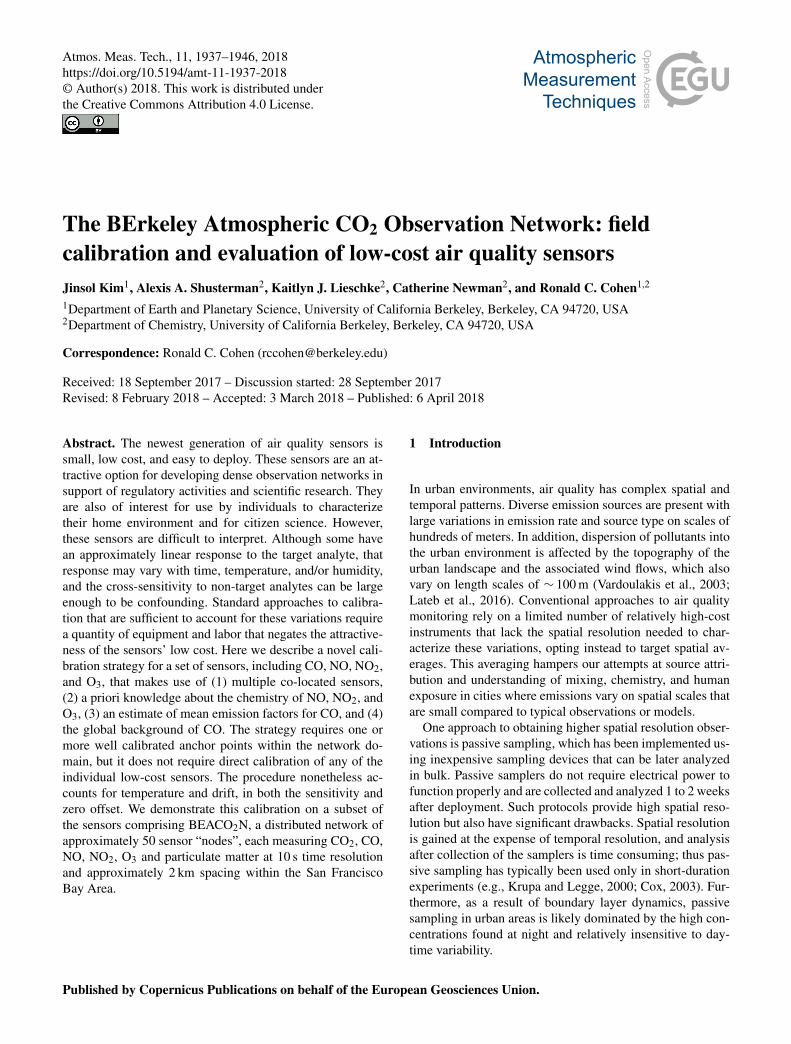
Figure 2. (a) Current BEACO2N node design and (b) a photo of anode deployed.

Recent developments in low-cost sensors for trace gasesand particulate matter, as well as advances in softwareand hardware enabling low-cost data communication, havemade high-density, high-time-resolution air quality monitor-ing networks possible. Devices and networks of devices areemerging that are low cost, report at a time resolution of sec-onds, and are capable of long-term deployment, providingpotential for improvement over the two major weaknessesof passive sampling. Examples include metal oxide sensorsused to measure O3, CO, NO2, and total volatile organiccompounds (e.g., Williams et al., 2013; Bart et al., 2014;Piedrahita et al., 2014; Moltchanov et al., 2015; Sadighi etal., 2017), and electrochemical sensors used to measure CO,NO, NO2, O3, and SO2 (e.g., Mead et al., 2013; Sun et al.,2015; Jiao et al., 2016; Hagan et al., 2017; Jerrett et al., 2017;Mueller et al., 2017). These different low-cost sensor systemshave been evaluated and compared (Borrego et al., 2016; Pa-papostolou et al., 2017). While these studies found low-costtrace gas sensors to be successful at qualitatively characteriz-ing the variability of air quality in an urban area, challenges

related to selectivity and stability remain, hindering morequantitative interpretation of the data.

The current generation of low-cost sensors is not as easilytied to a gravimetric calibration standard as many of the pas-sive samplers. Calibration is known to vary with sensor age,temperature, and in some cases humidity. In addition, manyof the sensors have responses to gases other than the targetanalyte (Mead et al., 2013; Spinelle et al., 2015, 2017; Crosset al., 2017; Mueller et al., 2017; Mijling et al., 2018; Zim-merman et al., 2018). One approach to addressing this chal-lenge is to combine periodic re-calibration and co-locationwith regulatory reference instruments in the lab or the field(Williams et al., 2013; Moltchanov et al., 2015; Jiao et al.,2016; Mijling et al., 2018). Field calibration is preferred asin-lab performance is often a poor approximation of sensorbehavior under ambient conditions (Piedrahita et al., 2014;Masson et al., 2015). However, either method requires con-siderable time investment by trained personnel, especially asthe number of sensors increases. The requirement of time-consuming and labor-intensive calibration then offsets thelow-cost advantage of the sensors.

In this paper, we explore an automated, in situ strategyfor the calibration of individual sensors embedded in anair quality sensor network that includes both low-cost sen-sors and anchor points of higher-grade, well-calibrated in-strumentation. The BErkeley Atmospheric CO2 ObservationNetwork (BEACO2N) is a low-cost, high-density greenhousegas (CO2) and air quality (CO, NO, NO2, O3, and partic-ulate matter) monitoring network located in San FranciscoBay Area, California (see Fig. 1 and Shusterman et al., 2016).As of this writing, BEACO2N consists of approximately 50sensor “nodes”, deployed with approximately 2 km horizon-tal spacing. Most of the nodes are mounted on the roofs ofschools and museums. In previous work, we described anapproach to CO2 sensing and calibration (Shusterman et al.,2016). Here, we focus on CO, NO, NO2, and O3.

Atmos. Meas. Tech., 11, 1937–1946, 2018 www.atmos-meas-tech.net/11/1937/2018/

J. Kim et al.: BErkeley Atmospheric CO2 Observation Network 1939

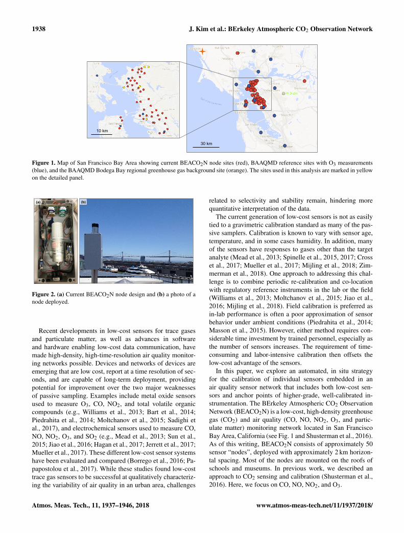
Figure 3. Representative temperature-dependent sensitivities (a)and zero offsets (b) of the Alphasense electrochemical sensors cal-culated by comparing hourly averaged measurements from LaneyCollege BEACO2N node to measurements from a co-located refer-ence instrument during February to April 2016.

We begin by describing laboratory experiments and in-field comparisons to co-located reference instruments thatgive an initial characterization of the sensors and provideinsight into the effects of temperature, humidity, and cross-sensitivity to non-target analytes. Then we describe an insitu calibration procedure that accounts for these variableswithout requiring co-location with a reference instrument.The calibration procedure is finally verified against regula-tory quality measurements not used in the procedure itself.

2 Instrument description

Details of the node design and deployment are described inShusterman et al. (2016). Briefly, each BEACO2N node con-tains a Vaisala CarboCap GMP343 non-dispersive infraredsensor for CO2, a Shinyei PPD42NS nephelometric particu-late matter sensor, and a suite of Alphasense electrochemicalsensors: CO-B4, NO-B4, either NO2-B42F or NO2-B43F,and either Ox-B421 or Ox-B431. All sensors are assembledinto compact, weatherproof enclosures as shown in Fig. 2.Two 30 mm fans are located on either side of the enclosureto facilitate airflow through the node. A Raspberry Pi micro-processor collects data via a serial-to-USB converter for CO2and an Adafruit Metro Mini microcontroller for all other sen-sors. Then, data collected every 5 or 10 s are transmitted to acentral server using a direct on-site Ethernet connection or alocal Wi-Fi network.

The Alphasense B4 electrochemical gas sensing series thatwe use employs a four-electrode approach. The electrodesare embedded in an electrolyte solution separated from theatmosphere by a semi-permeable membrane. The gas of in-terest diffuses through the membrane into the electrolyte,

where it contacts a “working” electrode and is either oxi-dized (in the case of NO and CO) or reduced (NO2 and O3).The potential at the working electrode is maintained at a con-stant value with respect to a “reference” electrode. Electriccharge produced at the working electrode is balanced by thecomplementary redox reaction at a “counter” electrode, gen-erating an electric current. The sensor also contains an “aux-iliary” electrode, which shares the working electrode’s cata-lyst structure, but is isolated from the ambient environment,accounting for fluctuations in the background current asso-ciated with other processes at the electrode and electrolyte.Subtracting the auxiliary current from the working currentgives a corrected current dependent on the gas concentration.

The working and auxiliary currents detected by the sen-sors are converted to working and auxiliary voltages usingamplifiers in the individual sensor boards (ISBs) providedby Alphasense. Over the mixing ratio range of interest, thesensors’ responses to the gases of interest are approximatelylinear. We derive mixing ratios from the observed voltages bysubtracting an offset and then scaling by a constant (Eqs. 1–4):

COambient = (VCO-zeroCO)/kCO, (1)NOambient = (VNO-zeroNO)/kNO, (2)

NO2ambient = (VNO2 -zeroNO2)/kNO2

− (rNO-NO2 ×NOambient), (3a)NO2ambient = (VNO2 -zeroNO2)/kNO2

+ (rCO2-NO2 ×CO2ambient), (3b)

O3ambient = (VO3 -zeroO3)/kO3 − (rNO2-O3 ×NO2ambient). (4)

Here, CO, NO, NO2, and O3 with the subscript “ambient” re-fer to the gas mixing ratios (ppb) in air; VCO, VNO, VNO2 andVO3 are the signals (mV) measured by each sensor, whichis the voltage of the auxiliary electrode subtracted from thevoltage of the working electrode; zeroCO, zeroNO, zeroNO2

and zeroO3 indicates the voltage measured in the absenceof analyte; and kCO, kNO, kNO2 and kO3 represent the linearsensitivity factor that converts mV to ppb. Additional termscorresponding to the cross-sensitivities of the NO2 and O3sensors appear in Eqs. (3a), (3b), and (4), where rNO-NO2

is the cross-sensitivity of the NO2-B42F sensor to NO gas,rCO2-NO2 is the cross-sensitivity of the NO2-B43F sensor toCO2 gas, and rNO2-O3 is the cross-sensitivity of both the O3-B421 and O3-B431 sensors to NO2 gas.

There are a total of eight sensitivities and zero offsets, aswell as two cross-sensitivity terms. All of these may also varywith time, temperature, and humidity. Thus we need a cali-bration strategy that constrains 10 parameters in a single in-stant as well as the variation of those 10 parameters in re-sponse to the environmental variables and time. We begin bycharacterizing the sensors in both laboratory and outdoor en-vironments.

www.atmos-meas-tech.net/11/1937/2018/ Atmos. Meas. Tech., 11, 1937–1946, 2018

1940 J. Kim et al.: BErkeley Atmospheric CO2 Observation Network

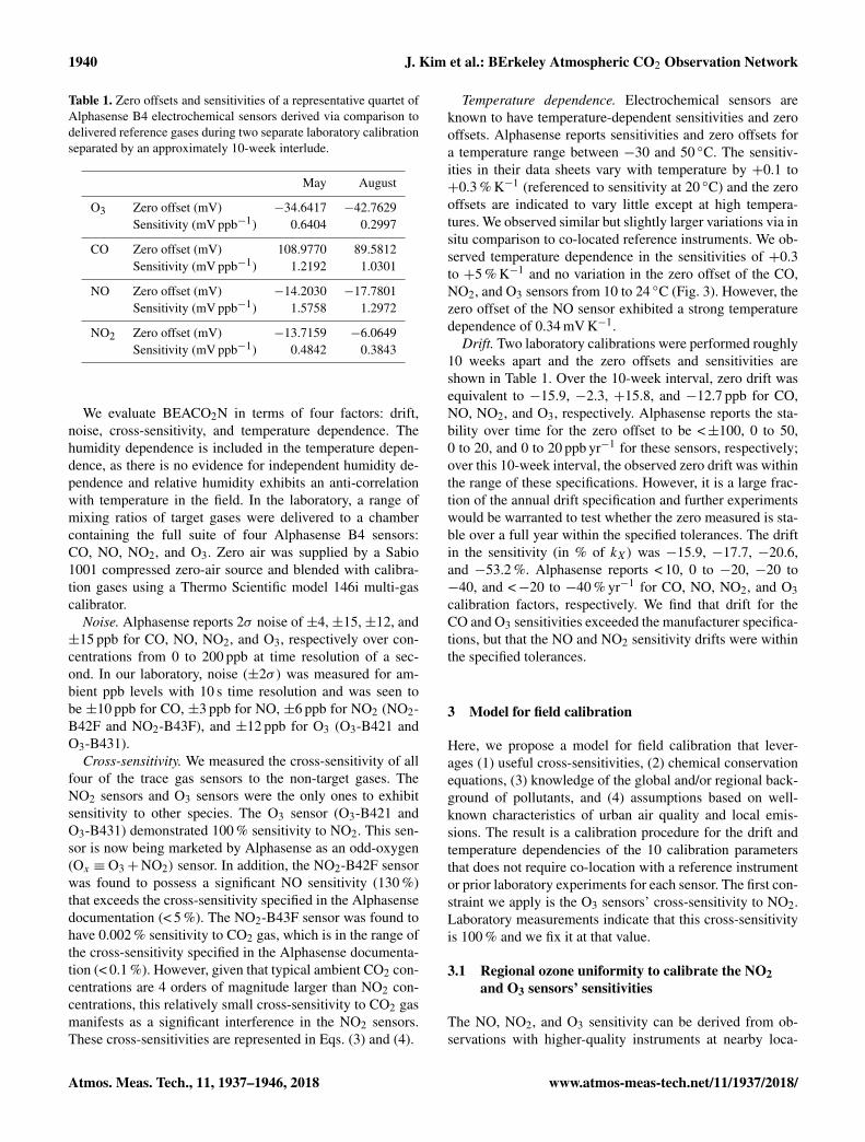
Table 1. Zero offsets and sensitivities of a representative quartet ofAlphasense B4 electrochemical sensors derived via comparison todelivered reference gases during two separate laboratory calibrationseparated by an approximately 10-week interlude.

May August

O3 Zero offset (mV) −34.6417 −42.7629Sensitivity (mV ppb−1) 0.6404 0.2997

CO Zero offset (mV) 108.9770 89.5812Sensitivity (mV ppb−1) 1.2192 1.0301

NO Zero offset (mV) −14.2030 −17.7801Sensitivity (mV ppb−1) 1.5758 1.2972

NO2 Zero offset (mV) −13.7159 −6.0649Sensitivity (mV ppb−1) 0.4842 0.3843

We evaluate BEACO2N in terms of four factors: drift,noise, cross-sensitivity, and temperature dependence. Thehumidity dependence is included in the temperature depen-dence, as there is no evidence for independent humidity de-pendence and relative humidity exhibits an anti-correlationwith temperature in the field. In the laboratory, a range ofmixing ratios of target gases were delivered to a chambercontaining the full suite of four Alphasense B4 sensors:CO, NO, NO2, and O3. Zero air was supplied by a Sabio1001 compressed zero-air source and blended with calibra-tion gases using a Thermo Scientific model 146i multi-gascalibrator.

Noise. Alphasense reports 2σ noise of ±4, ±15, ±12, and±15 ppb for CO, NO, NO2, and O3, respectively over con-centrations from 0 to 200 ppb at time resolution of a sec-ond. In our laboratory, noise (±2σ) was measured for am-bient ppb levels with 10 s time resolution and was seen tobe ±10 ppb for CO, ±3 ppb for NO, ±6 ppb for NO2 (NO2-B42F and NO2-B43F), and ±12 ppb for O3 (O3-B421 andO3-B431).

Cross-sensitivity. We measured the cross-sensitivity of allfour of the trace gas sensors to the non-target gases. TheNO2 sensors and O3 sensors were the only ones to exhibitsensitivity to other species. The O3 sensor (O3-B421 andO3-B431) demonstrated 100 % sensitivity to NO2. This sen-sor is now being marketed by Alphasense as an odd-oxygen(Ox ≡ O3+NO2) sensor. In addition, the NO2-B42F sensorwas found to possess a significant NO sensitivity (130 %)that exceeds the cross-sensitivity specified in the Alphasensedocumentation (< 5 %). The NO2-B43F sensor was found tohave 0.002 % sensitivity to CO2 gas, which is in the range ofthe cross-sensitivity specified in the Alphasense documenta-tion (< 0.1 %). However, given that typical ambient CO2 con-centrations are 4 orders of magnitude larger than NO2 con-centrations, this relatively small cross-sensitivity to CO2 gasmanifests as a significant interference in the NO2 sensors.These cross-sensitivities are represented in Eqs. (3) and (4).

Temperature dependence. Electrochemical sensors areknown to have temperature-dependent sensitivities and zerooffsets. Alphasense reports sensitivities and zero offsets fora temperature range between −30 and 50 ◦C. The sensitiv-ities in their data sheets vary with temperature by +0.1 to+0.3 % K−1 (referenced to sensitivity at 20 ◦C) and the zerooffsets are indicated to vary little except at high tempera-tures. We observed similar but slightly larger variations via insitu comparison to co-located reference instruments. We ob-served temperature dependence in the sensitivities of +0.3to +5 % K−1 and no variation in the zero offset of the CO,NO2, and O3 sensors from 10 to 24 ◦C (Fig. 3). However, thezero offset of the NO sensor exhibited a strong temperaturedependence of 0.34 mV K−1.

Drift. Two laboratory calibrations were performed roughly10 weeks apart and the zero offsets and sensitivities areshown in Table 1. Over the 10-week interval, zero drift wasequivalent to −15.9, −2.3, +15.8, and −12.7 ppb for CO,NO, NO2, and O3, respectively. Alphasense reports the sta-bility over time for the zero offset to be <±100, 0 to 50,0 to 20, and 0 to 20 ppb yr−1 for these sensors, respectively;over this 10-week interval, the observed zero drift was withinthe range of these specifications. However, it is a large frac-tion of the annual drift specification and further experimentswould be warranted to test whether the zero measured is sta-ble over a full year within the specified tolerances. The driftin the sensitivity (in % of kX) was −15.9, −17.7, −20.6,and −53.2 %. Alphasense reports < 10, 0 to −20, −20 to−40, and <−20 to −40 % yr−1 for CO, NO, NO2, and O3calibration factors, respectively. We find that drift for theCO and O3 sensitivities exceeded the manufacturer specifica-tions, but that the NO and NO2 sensitivity drifts were withinthe specified tolerances.

3 Model for field calibration

Here, we propose a model for field calibration that lever-ages (1) useful cross-sensitivities, (2) chemical conservationequations, (3) knowledge of the global and/or regional back-ground of pollutants, and (4) assumptions based on well-known characteristics of urban air quality and local emis-sions. The result is a calibration procedure for the drift andtemperature dependencies of the 10 calibration parametersthat does not require co-location with a reference instrumentor prior laboratory experiments for each sensor. The first con-straint we apply is the O3 sensors’ cross-sensitivity to NO2.Laboratory measurements indicate that this cross-sensitivityis 100 % and we fix it at that value.

3.1 Regional ozone uniformity to calibrate the NO2and O3 sensors’ sensitivities

The NO, NO2, and O3 sensitivity can be derived from ob-servations with higher-quality instruments at nearby loca-

Atmos. Meas. Tech., 11, 1937–1946, 2018 www.atmos-meas-tech.net/11/1937/2018/

J. Kim et al.: BErkeley Atmospheric CO2 Observation Network 1941

Table 2. Reported emission factors of diesel and gasoline vehicles (Dallmann et al., 2011, 2012, 2013). Emissions from medium-duty andheavy-duty diesel trucks, which account for < 1 % of all vehicles, were removed to give the value for light-duty gasoline vehicles.

Vehicle type CO emission factor NOX emission factor(g kg fuel−1) (g kg fuel−1)

Heavy-duty diesel trucks 8.0± 1.2 28.0± 1.5Light-duty gasoline vehicles 14.3± 0.7 1.90± 0.0899 % gasoline vehicles, 1 % diesel trucks 14.2± 0.7 2.29± 0.12

Table 3. Mean absolute error of comparison between regional O3 and hourly averaged BEACO2N O3 measurements derived from multiplelinear regression models of increasing complexity between February and April 2016.

Regression Models Mean absolute error(ppb)

O3true =VO3kO3− offset Linearity of observed voltages and gas concentration 14.4063

O3true =VO3kO3−VNO2kNO2− offset O3 sensor’s cross-sensitivity correction 10.6795

O3true =VO3kO3−VNO2kNO2+ rNO-NO2

VNOkNO− offset NO2 and O3 sensor’s cross-sensitivity correction 8.8172

O3true =VO3kO3−VNO2kNO2+ rNO-NO2

VNOkNO− offset Adding temperature correction 8.1360

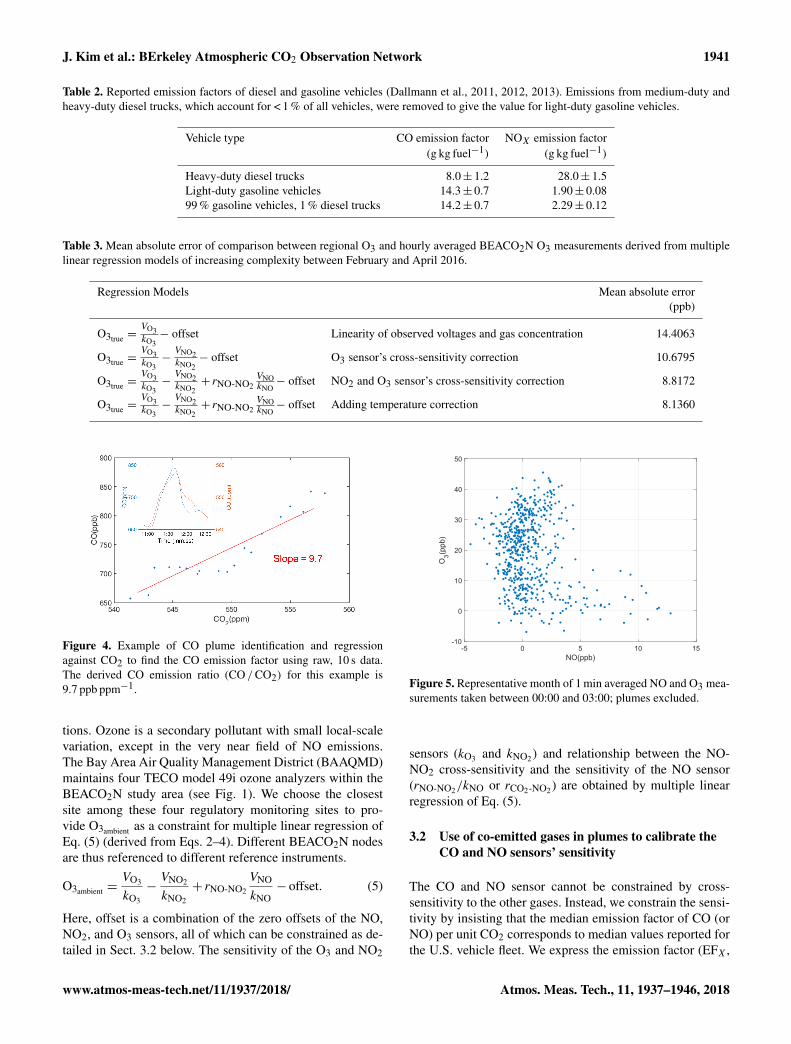
Figure 4. Example of CO plume identification and regressionagainst CO2 to find the CO emission factor using raw, 10 s data.The derived CO emission ratio (CO /CO2) for this example is9.7 ppb ppm−1.

tions. Ozone is a secondary pollutant with small local-scalevariation, except in the very near field of NO emissions.The Bay Area Air Quality Management District (BAAQMD)maintains four TECO model 49i ozone analyzers within theBEACO2N study area (see Fig. 1). We choose the closestsite among these four regulatory monitoring sites to pro-vide O3ambient as a constraint for multiple linear regression ofEq. (5) (derived from Eqs. 2–4). Different BEACO2N nodesare thus referenced to different reference instruments.

O3ambient =VO3

kO3

−VNO2

kNO2

+ rNO-NO2

VNO

kNO− offset. (5)

Here, offset is a combination of the zero offsets of the NO,NO2, and O3 sensors, all of which can be constrained as de-tailed in Sect. 3.2 below. The sensitivity of the O3 and NO2

-5 0 5 10 15NO(ppb)

-10

0

10

20

30

40

50

O3(p

pb)

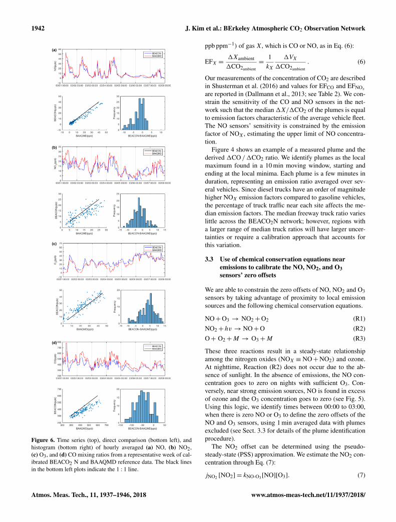
Figure 5. Representative month of 1 min averaged NO and O3 mea-surements taken between 00:00 and 03:00; plumes excluded.

sensors (kO3 and kNO2) and relationship between the NO-NO2 cross-sensitivity and the sensitivity of the NO sensor(rNO-NO2/kNO or rCO2-NO2 ) are obtained by multiple linearregression of Eq. (5).

3.2 Use of co-emitted gases in plumes to calibrate theCO and NO sensors’ sensitivity

The CO and NO sensor cannot be constrained by cross-sensitivity to the other gases. Instead, we constrain the sensi-tivity by insisting that the median emission factor of CO (orNO) per unit CO2 corresponds to median values reported forthe U.S. vehicle fleet. We express the emission factor (EFX,

www.atmos-meas-tech.net/11/1937/2018/ Atmos. Meas. Tech., 11, 1937–1946, 2018

1942 J. Kim et al.: BErkeley Atmospheric CO2 Observation Network

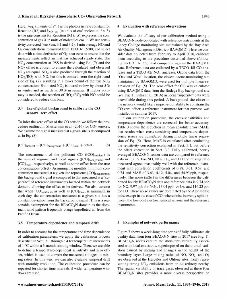
Figure 6. Time series (top), direct comparison (bottom left), andhistogram (bottom right) of hourly averaged (a) NO, (b) NO2,(c) O3, and (d) CO mixing ratios from a representative week of cal-ibrated BEACO2 N and BAAQMD reference data. The black linesin the bottom left plots indicate the 1 : 1 line.

ppb ppm−1) of gas X, which is CO or NO, as in Eq. (6):

EFX =1Xambient

1CO2ambient

=1kX

1VX

1CO2ambient

. (6)

Our measurements of the concentration of CO2 are describedin Shusterman et al. (2016) and values for EFCO and EFNOxare reported in (Dallmann et al., 2013; see Table 2). We con-strain the sensitivity of the CO and NO sensors in the net-work such that the median1X/1CO2 of the plumes is equalto emission factors characteristic of the average vehicle fleet.The NO sensors’ sensitivity is constrained by the emissionfactor of NOX, estimating the upper limit of NO concentra-tion.

Figure 4 shows an example of a measured plume and thederived 1CO /1CO2 ratio. We identify plumes as the localmaximum found in a 10 min moving window, starting andending at the local minima. Each plume is a few minutes induration, representing an emission ratio averaged over sev-eral vehicles. Since diesel trucks have an order of magnitudehigher NOX emission factors compared to gasoline vehicles,the percentage of truck traffic near each site affects the me-dian emission factors. The median freeway truck ratio varieslittle across the BEACO2N network; however, regions witha larger range of median truck ratios will have larger uncer-tainties or require a calibration approach that accounts forthis variation.

3.3 Use of chemical conservation equations nearemissions to calibrate the NO, NO2, and O3sensors’ zero offsets

We are able to constrain the zero offsets of NO, NO2 and O3sensors by taking advantage of proximity to local emissionsources and the following chemical conservation equations.

NO+O3 → NO2+O2 (R1)NO2+hv → NO+O (R2)O+ O2+M → O3+M (R3)

These three reactions result in a steady-state relationshipamong the nitrogen oxides (NOX ≡ NO+NO2) and ozone.At nighttime, Reaction (R2) does not occur due to the ab-sence of sunlight. In the absence of emissions, the NO con-centration goes to zero on nights with sufficient O3. Con-versely, near strong emission sources, NO is found in excessof ozone and the O3 concentration goes to zero (see Fig. 5).Using this logic, we identify times between 00:00 to 03:00,when there is zero NO or O3 to define the zero offsets of theNO and O3 sensors, using 1 min averaged data with plumesexcluded (see Sect. 3.3 for details of the plume identificationprocedure).

The NO2 offset can be determined using the pseudo-steady-state (PSS) approximation. We estimate the NO2 con-centration through Eq. (7):

jNO2 [NO2]= kNO-O3 [NO][O3]. (7)

Atmos. Meas. Tech., 11, 1937–1946, 2018 www.atmos-meas-tech.net/11/1937/2018/

J. Kim et al.: BErkeley Atmospheric CO2 Observation Network 1943

Here, jNO2 (in units of s−1) is the photolysis rate constant forReaction (R2) and kNO−O3 (in units of cm3 molecule−1 s−1)

is the rate constant for Reaction (R1). [X] expresses the con-centration of gasX in units of molecules cm−3. We use sensi-tivity corrected (see Sect. 3.1 and 3.2), 1 min average NO andO3 concentrations measured from 12:00 to 15:00, and selectdata with a time derivative of O3 near zero to ensure that themeasurements reflect air that has achieved steady state. TheNO2 concentration at PSS is derived using Eq. (7) and theNO2 offset is chosen to ensure the calculated and observedNO2 are equal. NO2 is also produced through the reaction ofHO2/RO2 with NO, but this is omitted from the right-handside of Eq. (7), resulting in a lower bound of the true NO2concentration. Estimated NO2 is therefore low by about 5 %in winter and as much as 30 % in summer. If higher accu-racy is needed, the reaction of HO2/RO2 with NO could beconsidered to reduce this bias.

3.4 Use of global background to calibrate the COsensors’ zero offset

To infer the zero offset of the CO sensor, we follow the pro-cedure outlined in Shusterman et al. (2016) for CO2 sensors.We assume the signal measured at a given site is decomposedas in Eq. (8):

[CO]ambient = [CO]background+ [CO]local+ offset. (8)

The measurement of the pollutant CO ([CO]ambient) isthe sum of regional and local signals ([CO]background and[CO]local, respectively), as well as some offset from the trueconcentration (offset). Assuming the monthly minimum con-centration measured at a given site represents [CO]background,this background signal is compared to that measured at a “su-persite” of reference instruments located within the networkdomain, allowing the offset to be derived. We also assumethat when [CO]ambient, as well as [CO]local, is minimum ineach day, the concentration measured at a given site has aconstant deviation from the background signal. This is a rea-sonable assumption for the BEACO2N domain as the dom-inant wind pattern frequently brings unpolluted air from thePacific Ocean.

3.5 Temperature dependence and temporal drift

In order to account for the temperature and time dependenceof calibration parameters, we apply the calibration processdescribed in Sect. 3.1 through 3.4 for temperature incrementsof 1 ◦C within a 3-month running window. Then, we are ableto define a temperature-dependent sensitivity and zero off-set, which is used to convert the measured voltages to mix-ing ratios. In this way, we can also evaluate temporal driftwith monthly resolution. The calibration procedure can berepeated for shorter time intervals if wider temperature win-dows are used.

4 Evaluation with reference observations

We evaluate the efficacy of our calibration method using aBEACO2N node co-located with reference instruments at theLaney College monitoring site maintained by the Bay AreaAir Quality Management District (BAAQMD). Here we con-sider data collected from February to April 2016, calibratethem according to the procedure described above (follow-ing Sect. 3.1 to 3.5), and compare it against the BAAQMDdata. Reference data are collected by a TECO 48i CO ana-lyzer and a TECO 42i NOx analyzer. Ozone data from the“Oakland West” location, the closest ozone-monitoring sitemaintained by BAAQMD, were used for multiple linear re-gression of Eq. (5). The zero offset for CO was calculatedusing BAAQMD data from the Bodega Bay background site(see Fig. 1; Guha et al., 2016) as local “supersite” data wereunavailable during this period. A background site closer tothe network would likely improve our ability to constrain theCO zero offset; a reference instrument for that purpose wasinstalled in summer 2017.

In our calibration procedure, the cross-sensitivities andtemperature dependence are corrected for better accuracy.Table 3 shows the reduction in mean absolute error (MAE)that results when cross-sensitivity and temperature depen-dence issues are considered during multiple linear regres-sion of Eq. (5). Here, MAE is calculated after conductingthe sensitivity correction explained in Sect. 3.1, but beforethe offset correction in Sect. 3.3. Fully calibrated, hourlyaveraged BEACO2N sensor data are compared to referencedata in Fig. 6. For NO, NO2, O3, and CO the mixing ratiomeasured agrees reasonably well with the reference instru-ment with correlation coefficients of 0.88, 0.61, 0.69, and0.74 and MAE of 3.63, 4.12, 5.04, and 54.93 ppb, respec-tively. The noise (±2σ) in the differences between the cali-brated hourly BEACO2N data and reference data is 9.74 ppbfor NO, 9.97 ppb for NO2, 13.04 ppb for O3, and 116.23 ppbfor CO. These noise values are dominated by the Alphasensenoise except in the case of CO, where noise is evenly split be-tween the low-cost electrochemical sensors and the referenceinstruments.

5 Examples of network performance

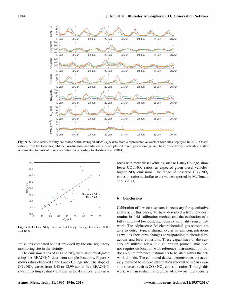
Figure 7 shows a week-long time series of fully calibrated airquality data from four BEACO2N sites in 2017 (see Fig. 1).BEACO2N nodes capture the short-term variability associ-ated with local emissions, superimposed on the diurnal vari-ation caused by mixing and changes in the height of theboundary layer. Large mixing ratios of NO, NO2, and O3are observed at the Hercules and Ohlone sites, likely repre-senting strong NOx emissions from an oil refinery nearby.The spatial variability of trace gases observed at these fourBEACO2N sites provides a more diverse perspective on

www.atmos-meas-tech.net/11/1937/2018/ Atmos. Meas. Tech., 11, 1937–1946, 2018

1944 J. Kim et al.: BErkeley Atmospheric CO2 Observation Network

19 Jun 20 Jun 21 Jun 22 Jun 23 Jun 24 Jun 25 Jun 26 Jun20304050

Tem

p(°C

) 19 Jun 20 Jun 21 Jun 22 Jun 23 Jun 24 Jun 25 Jun 26 Jun

400450500550

CO

2(ppm

)

19 Jun 20 Jun 21 Jun 22 Jun 23 Jun 24 Jun 25 Jun 26 Jun0

200400600

CO

(ppb

)

19 Jun 20 Jun 21 Jun 22 Jun 23 Jun 24 Jun 25 Jun 26 Jun0

204060

NO

(ppb

)

19 Jun 20 Jun 21 Jun 22 Jun 23 Jun 24 Jun 25 Jun 26 Jun0

50100150

NO

2(ppb

)

19 Jun 20 Jun 21 Jun 22 Jun 23 Jun 24 Jun 25 Jun 26 Jun0

306090

O3(p

pb)

19 Jun 20 Jun 21 Jun 22 Jun 23 Jun 24 Jun 25 Jun 26 Jun0

102030

PM(

g m

)-3

Figure 7. Time series of fully calibrated 5 min averaged BEACO2N data from a representative week at four sites deployed in 2017. Obser-vations from the Hercules, Ohlone, Washington, and Madera sites are plotted in red, green, orange, and blue, respectively. Particulate matteris converted to units of mass concentration according to Holstius et al. (2014).

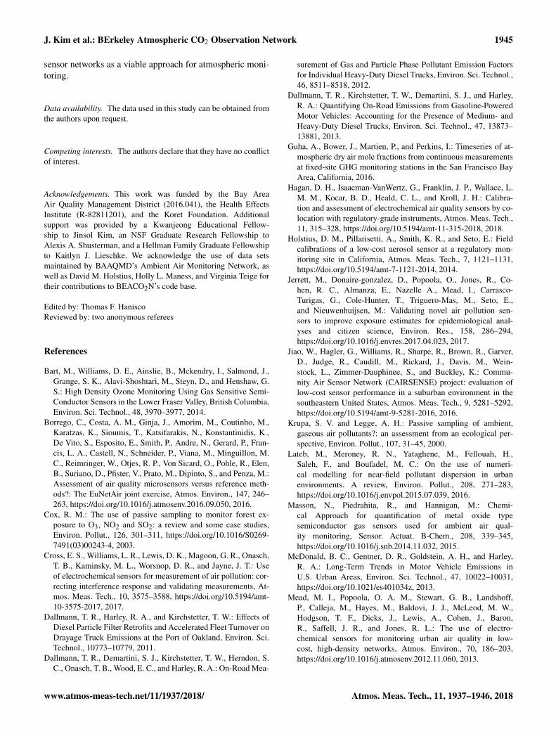
Slope = 4.34 R2 = 0.67

Figure 8. CO vs. NOx measured at Laney College between 08:00and 10:00.

emissions compared to that provided by the one regulatorymonitoring site in the vicinity.

The emission ratios of CO and NOx were also investigatedusing the BEACO2N data from sample locations. Figure 8shows ratios observed at the Laney College site. The slope ofCO /NOx varies from 4.43 to 12.99 across five BEACO2Nsites, reflecting spatial variations in local sources. Sites near

roads with more diesel vehicles, such as Laney College, showlower CO /NOx ratios, as expected given diesel vehicles’higher NOx emissions. The range of observed CO /NOxemission ratios is similar to the values reported by McDonaldet al. (2013).

6 Conclusions

Calibration of low-cost sensors is necessary for quantitativeanalysis. In this paper, we have described a truly low cost,routine in-field calibration method and the evaluation of afully calibrated low-cost, high-density air quality sensor net-work. The Alphasense B4 electrochemical gas sensors areable to detect typical diurnal cycles in gas concentrationsas well as short-term changes corresponding to chemical re-actions and local emissions. These capabilities of the sen-sors are utilized for a field calibration protocol that doesnot require co-location with reference instrumentation, butdoes require reference instruments to be sited within the net-work domain. The calibrated dataset demonstrates the accu-racy required to resolve information relevant to urban emis-sion sources, such as CO /NOx emission ratios. Through thiswork, we can realize the promise of low-cost, high-density

Atmos. Meas. Tech., 11, 1937–1946, 2018 www.atmos-meas-tech.net/11/1937/2018/

J. Kim et al.: BErkeley Atmospheric CO2 Observation Network 1945

sensor networks as a viable approach for atmospheric moni-toring.

Data availability. The data used in this study can be obtained fromthe authors upon request.

Competing interests. The authors declare that they have no conflictof interest.

Acknowledgements. This work was funded by the Bay AreaAir Quality Management District (2016.041), the Health EffectsInstitute (R-82811201), and the Koret Foundation. Additionalsupport was provided by a Kwanjeong Educational Fellow-ship to Jinsol Kim, an NSF Graduate Research Fellowship toAlexis A. Shusterman, and a Hellman Family Graduate Fellowshipto Kaitlyn J. Lieschke. We acknowledge the use of data setsmaintained by BAAQMD’s Ambient Air Monitoring Network, aswell as David M. Holstius, Holly L. Maness, and Virginia Teige fortheir contributions to BEACO2N’s code base.

Edited by: Thomas F. HaniscoReviewed by: two anonymous referees

References

Bart, M., Williams, D. E., Ainslie, B., Mckendry, I., Salmond, J.,Grange, S. K., Alavi-Shoshtari, M., Steyn, D., and Henshaw, G.S.: High Density Ozone Monitoring Using Gas Sensitive Semi-Conductor Sensors in the Lower Fraser Valley, British Columbia,Environ. Sci. Technol., 48, 3970–3977, 2014.

Borrego, C., Costa, A. M., Ginja, J., Amorim, M., Coutinho, M.,Karatzas, K., Sioumis, T., Katsifarakis, N., Konstantinidis, K.,De Vito, S., Esposito, E., Smith, P., Andre, N., Gerard, P., Fran-cis, L. A., Castell, N., Schneider, P., Viana, M., Minguillon, M.C., Reimringer, W., Otjes, R. P., Von Sicard, O., Pohle, R., Elen,B., Suriano, D., Pfister, V., Prato, M., Dipinto, S., and Penza, M.:Assessment of air quality microsensors versus reference meth-ods?: The EuNetAir joint exercise, Atmos. Environ., 147, 246–263, https://doi.org/10.1016/j.atmosenv.2016.09.050, 2016.

Cox, R. M.: The use of passive sampling to monitor forest ex-posure to O3, NO2 and SO2: a review and some case studies,Environ. Pollut., 126, 301–311, https://doi.org/10.1016/S0269-7491(03)00243-4, 2003.

Cross, E. S., Williams, L. R., Lewis, D. K., Magoon, G. R., Onasch,T. B., Kaminsky, M. L., Worsnop, D. R., and Jayne, J. T.: Useof electrochemical sensors for measurement of air pollution: cor-recting interference response and validating measurements, At-mos. Meas. Tech., 10, 3575–3588, https://doi.org/10.5194/amt-10-3575-2017, 2017.

Dallmann, T. R., Harley, R. A., and Kirchstetter, T. W.: Effects ofDiesel Particle Filter Retrofits and Accelerated Fleet Turnover onDrayage Truck Emissions at the Port of Oakland, Environ. Sci.Technol., 10773–10779, 2011.

Dallmann, T. R., Demartini, S. J., Kirchstetter, T. W., Herndon, S.C., Onasch, T. B., Wood, E. C., and Harley, R. A.: On-Road Mea-

surement of Gas and Particle Phase Pollutant Emission Factorsfor Individual Heavy-Duty Diesel Trucks, Environ. Sci. Technol.,46, 8511–8518, 2012.

Dallmann, T. R., Kirchstetter, T. W., Demartini, S. J., and Harley,R. A.: Quantifying On-Road Emissions from Gasoline-PoweredMotor Vehicles: Accounting for the Presence of Medium- andHeavy-Duty Diesel Trucks, Environ. Sci. Technol., 47, 13873–13881, 2013.

Guha, A., Bower, J., Martien, P., and Perkins, I.: Timeseries of at-mospheric dry air mole fractions from continuous measurementsat fixed-site GHG monitoring stations in the San Francisco BayArea, California, 2016.

Hagan, D. H., Isaacman-VanWertz, G., Franklin, J. P., Wallace, L.M. M., Kocar, B. D., Heald, C. L., and Kroll, J. H.: Calibra-tion and assessment of electrochemical air quality sensors by co-location with regulatory-grade instruments, Atmos. Meas. Tech.,11, 315–328, https://doi.org/10.5194/amt-11-315-2018, 2018.

Holstius, D. M., Pillarisetti, A., Smith, K. R., and Seto, E.: Fieldcalibrations of a low-cost aerosol sensor at a regulatory mon-itoring site in California, Atmos. Meas. Tech., 7, 1121–1131,https://doi.org/10.5194/amt-7-1121-2014, 2014.

Jerrett, M., Donaire-gonzalez, D., Popoola, O., Jones, R., Co-hen, R. C., Almanza, E., Nazelle A., Mead, I., Carrasco-Turigas, G., Cole-Hunter, T., Triguero-Mas, M., Seto, E.,and Nieuwenhuijsen, M.: Validating novel air pollution sen-sors to improve exposure estimates for epidemiological anal-yses and citizen science, Environ. Res., 158, 286–294,https://doi.org/10.1016/j.envres.2017.04.023, 2017.

Jiao, W., Hagler, G., Williams, R., Sharpe, R., Brown, R., Garver,D., Judge, R., Caudill, M., Rickard, J., Davis, M., Wein-stock, L., Zimmer-Dauphinee, S., and Buckley, K.: Commu-nity Air Sensor Network (CAIRSENSE) project: evaluation oflow-cost sensor performance in a suburban environment in thesoutheastern United States, Atmos. Meas. Tech., 9, 5281–5292,https://doi.org/10.5194/amt-9-5281-2016, 2016.

Krupa, S. V. and Legge, A. H.: Passive sampling of ambient,gaseous air pollutants?: an assessment from an ecological per-spective, Environ. Pollut., 107, 31–45, 2000.

Lateb, M., Meroney, R. N., Yataghene, M., Fellouah, H.,Saleh, F., and Boufadel, M. C.: On the use of numeri-cal modelling for near-field pollutant dispersion in urbanenvironments. A review, Environ. Pollut., 208, 271–283,https://doi.org/10.1016/j.envpol.2015.07.039, 2016.

Masson, N., Piedrahita, R., and Hannigan, M.: Chemi-cal Approach for quantification of metal oxide typesemiconductor gas sensors used for ambient air qual-ity monitoring, Sensor. Actuat. B-Chem., 208, 339–345,https://doi.org/10.1016/j.snb.2014.11.032, 2015.

McDonald, B. C., Gentner, D. R., Goldstein, A. H., and Harley,R. A.: Long-Term Trends in Motor Vehicle Emissions inU.S. Urban Areas, Environ. Sci. Technol., 47, 10022–10031,https://doi.org/10.1021/es401034z, 2013.

Mead, M. I., Popoola, O. A. M., Stewart, G. B., Landshoff,P., Calleja, M., Hayes, M., Baldovi, J. J., McLeod, M. W.,Hodgson, T. F., Dicks, J., Lewis, A., Cohen, J., Baron,R., Saffell, J. R., and Jones, R. L.: The use of electro-chemical sensors for monitoring urban air quality in low-cost, high-density networks, Atmos. Environ., 70, 186–203,https://doi.org/10.1016/j.atmosenv.2012.11.060, 2013.

www.atmos-meas-tech.net/11/1937/2018/ Atmos. Meas. Tech., 11, 1937–1946, 2018

1946 J. Kim et al.: BErkeley Atmospheric CO2 Observation Network

Mijling, B., Jiang, Q., de Jonge, D., and Bocconi, S.:Field calibration of electrochemical NO2 sensors in a cit-izen science context, Atmos. Meas. Tech., 11, 1297–1312,https://doi.org/10.5194/amt-11-1297-2018, 2018.

Moltchanov, S., Levy, I., Etzion, Y., Lerner, U., Broday, D. M., andFishbain, B.: On the feasibility of measuring urban air pollutionby wireless distributed sensor networks, Sci. Total Environ., 502,537–547, https://doi.org/10.1016/j.scitotenv.2014.09.059, 2015.

Mueller, M., Meyer, J., and Hueglin, C.: Design of an ozone andnitrogen dioxide sensor unit and its long-term operation withina sensor network in the city of Zurich, Atmos. Meas. Tech., 10,3783–3799, https://doi.org/10.5194/amt-10-3783-2017, 2017.

Papapostolou, V., Zhang, H., Feenstra, B. J., and Polidori,A.: Development of an environmental chamber for evalu-ating the performance of low-cost air quality sensors un-der controlled conditions, Atmos. Environ., 171, 82–90,https://doi.org/10.1016/j.atmosenv.2017.10.003, 2017.

Piedrahita, R., Xiang, Y., Masson, N., Ortega, J., Collier, A., Jiang,Y., Li, K., Dick, R. P., Lv, Q., Hannigan, M., and Shang, L.: Thenext generation of low-cost personal air quality sensors for quan-titative exposure monitoring, Atmos. Meas. Tech., 7, 3325–3336,https://doi.org/10.5194/amt-7-3325-2014, 2014.

Sadighi, K., Coffey, E., Polidori, A., Feenstra, B., Lv, Q., Henze,D. K., and Hannigan, M.: Intra-urban spatial variability of sur-face ozone and carbon dioxide in Riverside, CA: viability andvalidation of low-cost sensors, Atmos. Meas. Tech. Discuss.,https://doi.org/10.5194/amt-2017-183, in review, 2017.

Shusterman, A. A., Teige, V. E., Turner, A. J., Newman, C., Kim, J.,and Cohen, R. C.: The BErkeley Atmospheric CO2 ObservationNetwork: initial evaluation, Atmos. Chem. Phys., 16, 13449–13463, https://doi.org/10.5194/acp-16-13449-2016, 2016.

Spinelle, L., Gerboles, M., Gabriella, M., and Aleixandre, M.:Field calibration of a cluster of low-cost available sen-sors for air quality monitoring. Part A: Ozone and ni-trogen dioxide, Sensor. Actuat. B-Chem., 215, 249–257,https://doi.org/10.1016/j.snb.2015.03.031, 2015.

Spinelle, L., Gerboles, M., Gabriella, M., and Aleixandre,M.: Field calibration of a cluster of low-cost commer-cially available sensors for air quality monitoring. Part B:NO, CO and CO2, Sensor. Actuat. B-Chem., 238, 706–715,https://doi.org/10.1016/j.snb.2016.07.036, 2017.

Sun, L., Wong, K. C., Wei, P., Ye, S., Huang, H., and Yang, F.: De-velopment and Application of a Next Generation Air Sensor Net-work for the Hong Kong Marathon 2015 Air Quality Monitoring,Sensors, 16, 211, https://doi.org/10.3390/s16020211, 2015.

Vardoulakis, S., Fisher, B. E. A., Pericleous, K., and Gonzalez-flesca, N.: Modelling air quality in street canyons?: a review, At-mos. Environ., 37, 155–182, 2003.

Williams, D. E., Henshaw, G. S., Bart, M., Laing, G., Wag-ner, J., Naisbitt, S., and Salmond, J. A.: Validation of low-cost ozone measurement instruments suitable for use in an air-quality monitoring network, Meas. Sci. Technol., 24, 065803,https://doi.org/10.1088/0957-0233/24/6/065803, 2013.

Zimmerman, N., Presto, A. A., Kumar, S. P. N., Gu, J., Hauryliuk,A., Robinson, E. S., Robinson, A. L., and R. Subramanian: Amachine learning calibration model using random forests to im-prove sensor performance for lower-cost air quality monitoring,Atmos. Meas. Tech., 11, 291–313, https://doi.org/10.5194/amt-11-291-2018, 2018.

Atmos. Meas. Tech., 11, 1937–1946, 2018 www.atmos-meas-tech.net/11/1937/2018/