Embed Size (px)
Citation preview
The application of CALPHAD based tools to the Materials Genome
Initiative and ICME
Paul Mason
Thermo-Calc Software Inc.4160 Washington Road, Suite 230
McMurray, PA 15317
The 2008 National Academies report on Integrated Computational Materials Engineering (ICME) and President Obama's announcement of the Materials Genome Initiative (MGI) in June 2011 highlights the growing interest in using computational methods to aid materials design and process improvement.
For more than 30 years CALPHAD (CALculation of PHAse Diagrams) based tools have been used to accelerate alloy design and improve processes. CALPHAD is based on relating the underlying thermodynamics of a system to predict the phases that can form and the amounts and compositions of those phases in multicomponent systems of industrial relevance.
During this lecture, you will: - Discover how CALPHAD relates to ICME and MGI - Learn about the underlying concepts of the CALPHAD approach - See how CALPHAD-based computational tools may be applied in the materials life cycle for a range of different materials.
Goals of this lecture
There are three main sections to this lecture:
1. Describing what ICME, MGI and CALPHAD are and how CALPHAD fits into the larger ICME and MGI framework
2. A more detailed description of CALPHAD, CALPHAD based software tools and databases that underpin them.
3. Some practical examples of applications to the materials life cycle.
Outline
The National Academies Press, 2008
Integrated Computational Materials Engineering: A Transformational Discipline for Improved Competitiveness and National Security
What is ICME?
ICME: an approach to design products, the materials that comprise them, and their associated materials processing methods by linking materials models at multiple length scales. Key words are "Integrated", involving integrating models at multiple length scales, and "Engineering", signifying industrial utility.
Focus is on the materials, i.e. understanding how processes produce material structures, how those structures give rise to material properties, and how to select materials for a given application. This report describes the need for using multiscale materials modeling to capture the process-structures-properties-performance of a material.
What is MGI?
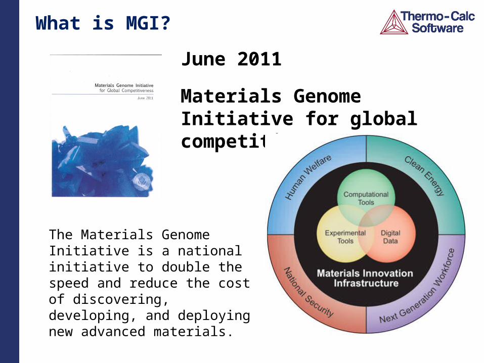
The Materials Genome Initiative is a national initiative to double the speed and reduce the cost of discovering, developing, and deploying new advanced materials.
June 2011
Materials Genome Initiative for global competitiveness
The influence of chemistry on microstructure and properties
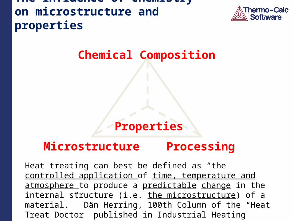
Heat treating can best be defined as “the controlled application of time, temperature and atmosphere to produce a predictable change in the internal structure (i.e. the microstructure) of a material.” Dan Herring, 100th Column of the “Heat Treat Doctor” published in Industrial Heating magazine
Chemical Composition
ProcessingMicrostructure
Properties
The analogy of a materials genome to a human genome implies that something of the nature of the material is encoded in the the chemical composition of a material and that we should be able to read this.
But nurture is important, as well as nature, and to extend the analogy further, nurture is the equivalent of processing the material.
In ICME/MGI we are striving to model how the structure and properties of a material are affected by its composition, synthesis, processing and usage.
Modelling of structure evolution and kinetic processes thus depends on what models are available for structure-property relations.
What should be modeled in the ICME and MGI?
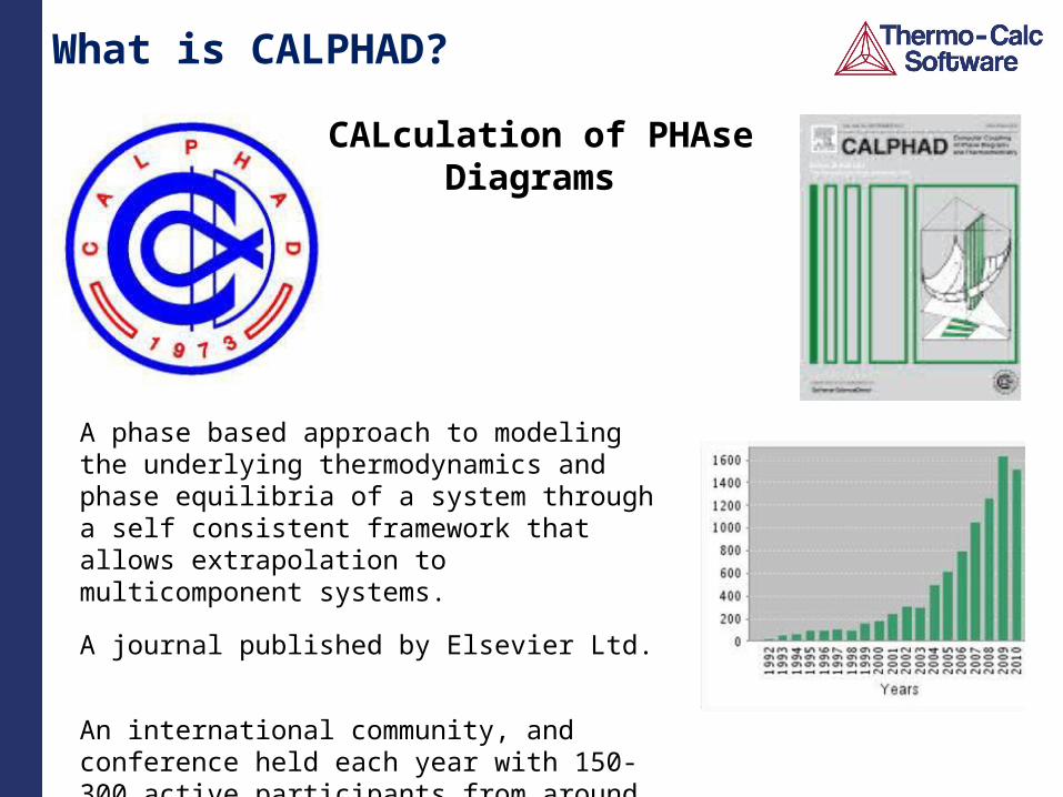
A phase based approach to modeling the underlying thermodynamics and phase equilibria of a system through a self consistent framework that allows extrapolation to multicomponent systems.
A journal published by Elsevier Ltd.
An international community, and conference held each year with 150-300 active participants from around the world.
What is CALPHAD?
CALculation of PHAse Diagrams
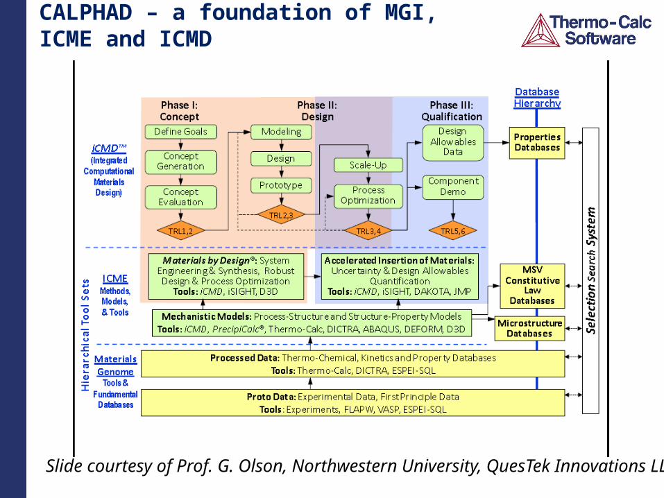
CALPHAD – a foundation of MGI, ICME and ICMD
Slide courtesy of Prof. G. Olson, Northwestern University, QuesTek Innovations LLC
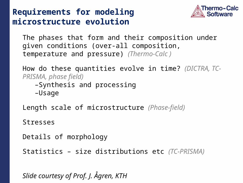
Requirements for modeling microstructure evolution
The phases that form and their composition under given conditions (over-all composition, temperature and pressure) (Thermo-Calc )
How do these quantities evolve in time? (DICTRA, TC-PRISMA, phase field)–Synthesis and processing –Usage
Length scale of microstructure (Phase-field)
Stresses
Details of morphology
Statistics – size distributions etc (TC-PRISMA)
Slide courtesy of Prof. J. Ågren, KTH
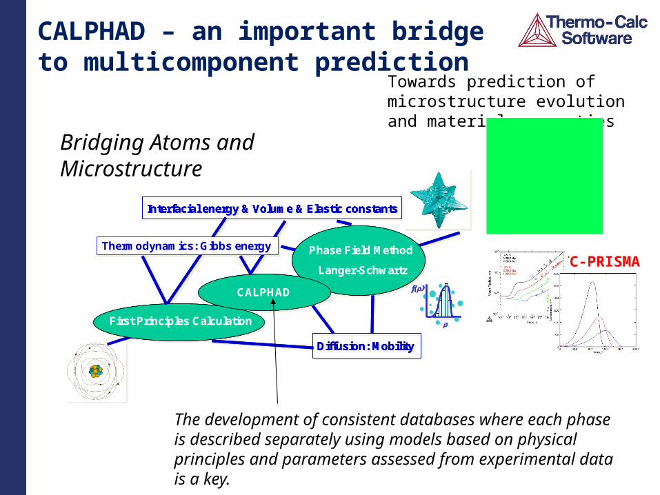
The development of consistent databases where each phase is described separately using models based on physical principles and parameters assessed from experimental data is a key.
CALPHAD – an important bridge to multicomponent prediction
Towards prediction of microstructure evolution and material properties
Bridging Atoms and Microstructure
Thermodynamics: Gibbs energy
Diffusion: Mobility
Phase Field Method
Langer-Schwartz
First Principles Calculation
CALPHAD f(
Interfacial energy & Volume & Elastic constants
Thermodynamics: Gibbs energy
Diffusion: MobilityDiffusion: Mobility
Phase Field Method
Langer-Schwartz
Phase Field Method
Langer-Schwartz
First Principles CalculationFirst Principles Calculation
CALPHADCALPHAD f(
f(
Interfacial energy & Volume & Elastic constantsInterfacial energy & Volume & Elastic constants
Thermodynamics: Gibbs energy
Diffusion: Mobility
Phase Field Method
Langer-Schwartz
First Principles Calculation
CALPHAD f(
Interfacial energy & Volume & Elastic constants
Thermodynamics: Gibbs energy
Diffusion: MobilityDiffusion: Mobility
Phase Field Method
Langer-Schwartz
Phase Field Method
Langer-Schwartz
First Principles CalculationFirst Principles Calculation
CALPHADCALPHAD f(
f(
Interfacial energy & Volume & Elastic constantsInterfacial energy & Volume & Elastic constants
TC-PRISMA
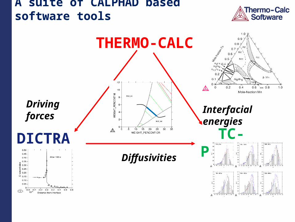
A suite of CALPHAD based software tools
THERMO-CALC
Diffusivities
x
x
DICTRA
Driving forces
TC-PRISMA
Interfacial energies
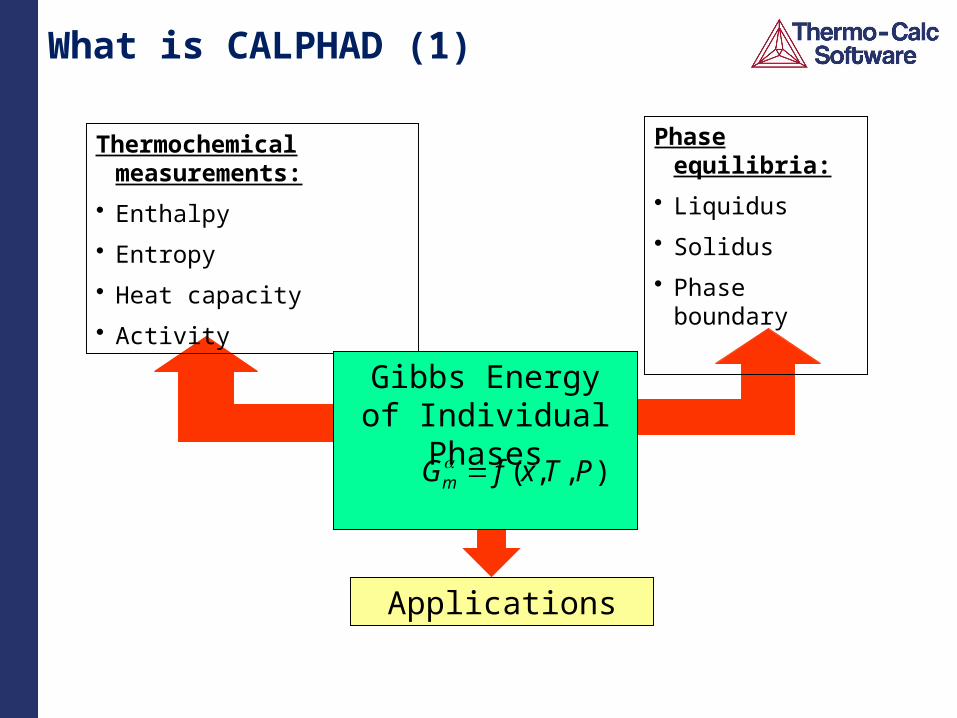
What is CALPHAD (1)
Thermochemical measurements:
• Enthalpy
• Entropy
• Heat capacity
• Activity
Phase equilibria:
• Liquidus
• Solidus
• Phase boundary
Gibbs Energy of Individual Phases
Applications
),,( PTxfGm
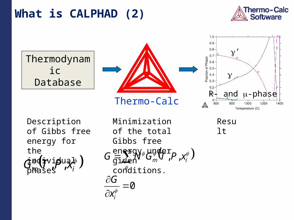
What is CALPHAD (2)
im xPTG ,,
Thermodynamic Database
Thermo-Calc
0
,,
i
im
x
G
xPTGNG
Description of Gibbs free energy for the individual phases
Minimization of the total Gibbs free energy under given conditions.
g’
g
R- and m-phase
Result
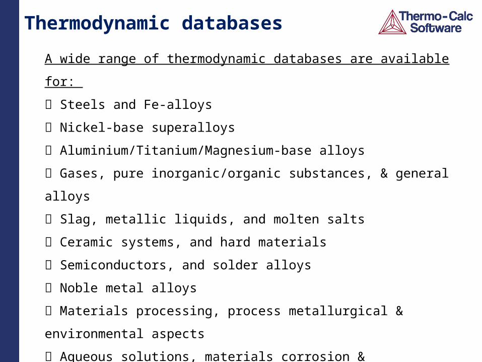
Thermodynamic databases
A wide range of thermodynamic databases are available for:
Steels and Fe-alloys
Nickel-base superalloys
Aluminium/Titanium/Magnesium-base alloys
Gases, pure inorganic/organic substances, & general alloys
Slag, metallic liquids, and molten salts
Ceramic systems, and hard materials
Semiconductors, and solder alloys
Noble metal alloys
Materials processing, process metallurgical & environmental aspects
Aqueous solutions, materials corrosion & hydrometallurgical systems
Minerals, and geochemical/environmental processes
Nuclear materials, and nuclear fuel/waste processing
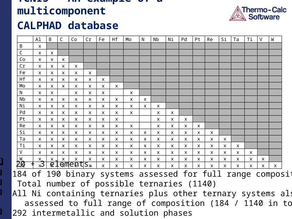
TCNI5 – An example of a multicomponent CALPHAD database
Al B C Co Cr Fe Hf Mo N Nb Ni Pd Pt Re Si Ta Ti V WB xC x xCo x x xCr x x x xFe x x x x xHf x x x x x xMo x x x x x x xN x x x x x xNb x x x x x x x x xNi x x x x x x x x x xPd x x x x x x x x x xPt x x x x x x x x x xRe x x x x x x x x x x x xSi x x x x x x x x x x x x x xTa x x x x x x x x x x x x x x xTi x x x x x x x x x x x x x x x xV x x x x x x x x x x x x x x x x xW x x x x x x x x x x x x x x x x x xZr x x x x x x x x x x x x x x x x x x x
20 + 3 elements. 184 of 190 binary systems assessed for full range composition Total number of possible ternaries (1140) All Ni containing ternaries plus other ternary systems also assessed to full range of composition (184 / 1140 in total) 292 intermetallic and solution phases
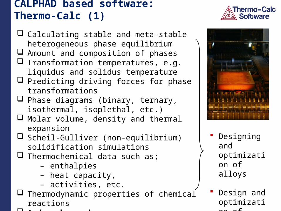
CALPHAD based software: Thermo-Calc (1)
Calculating stable and meta-stable heterogeneous phase equilibrium
Amount and composition of phases Transformation temperatures, e.g. liquidus and
solidus temperature Predicting driving forces for phase transformations Phase diagrams (binary, ternary, isothermal,
isoplethal, etc.) Molar volume, density and thermal expansion Scheil-Gulliver (non-equilibrium) solidification
simulations Thermochemical data such as;
– enthalpies – heat capacity, – activities, etc.
Thermodynamic properties of chemical reactions And much, much more….
Designing and optimization of alloys
Design and
optimization of processes
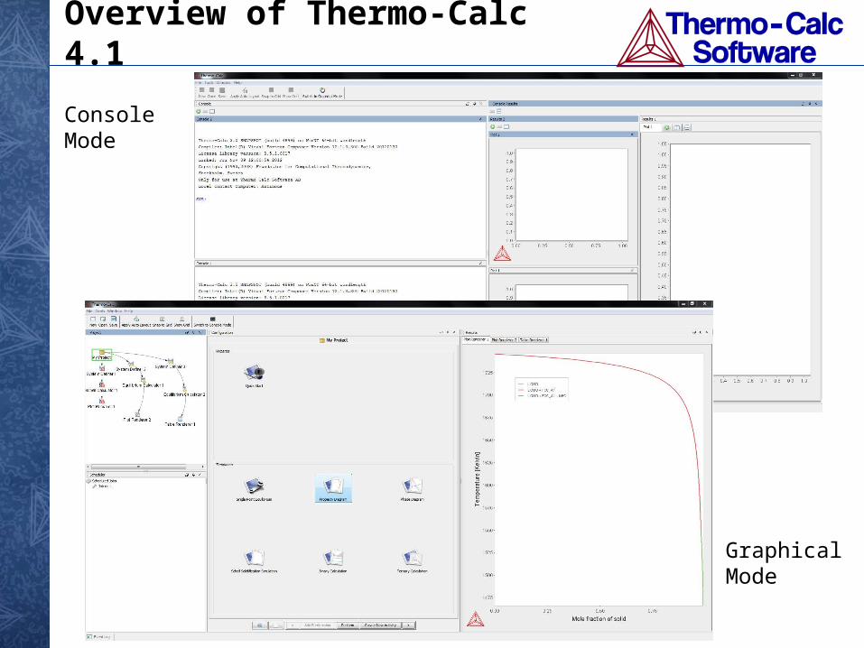
Overview of Thermo-Calc 4.1
Console Mode
Graphical Mode
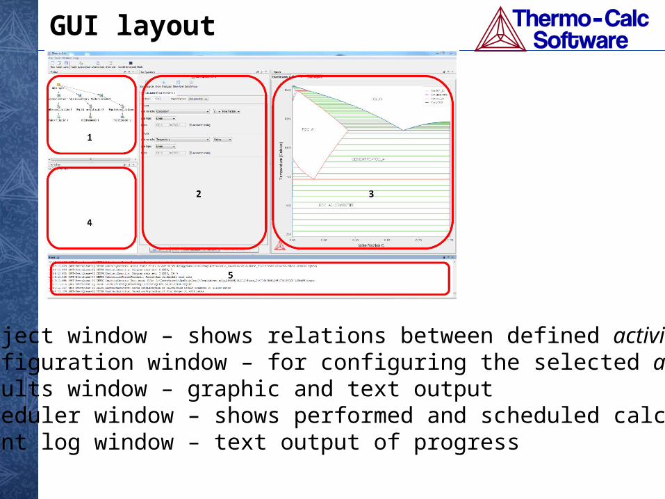
GUI layout
1. Project window – shows relations between defined activities2. Configuration window – for configuring the selected activity3. Results window – graphic and text output4. Scheduler window – shows performed and scheduled calculations5. Event log window – text output of progress
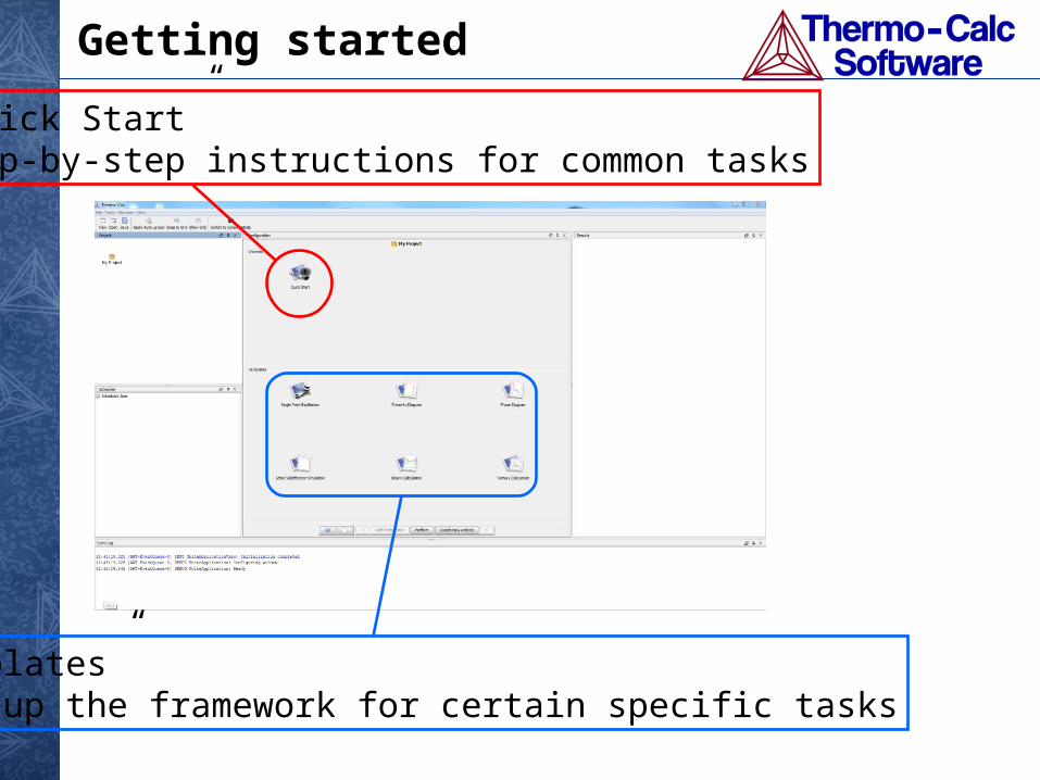
Getting started
”Quick Start”Step-by-step instructions for common tasks
”Templates”Sets up the framework for certain specific tasks
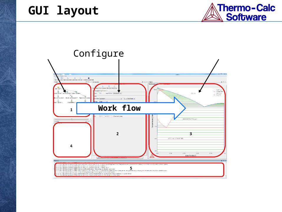
GUI layout
Work flow
Set-up Configure Results
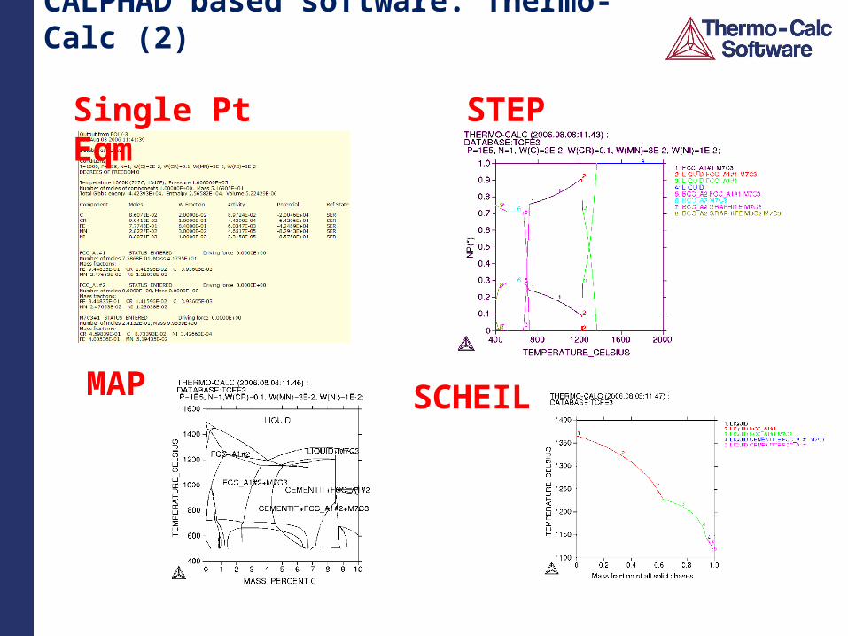
CALPHAD based software: Thermo-Calc (2)
Single Pt Eqm STEP
MAP SCHEIL
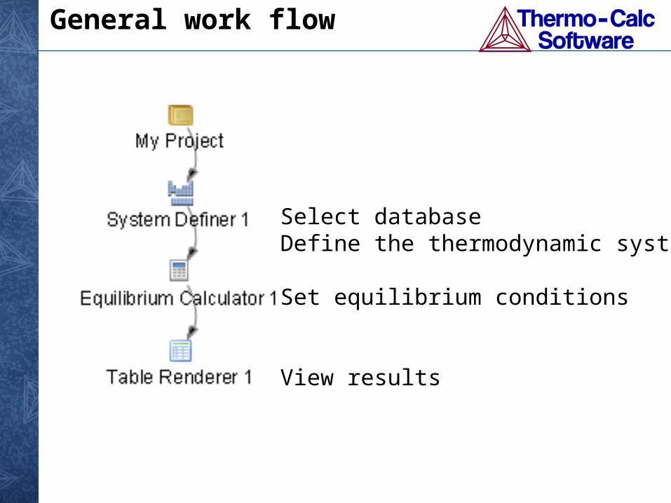
General work flow
Select databaseDefine the thermodynamic system
Set equilibrium conditions
View results
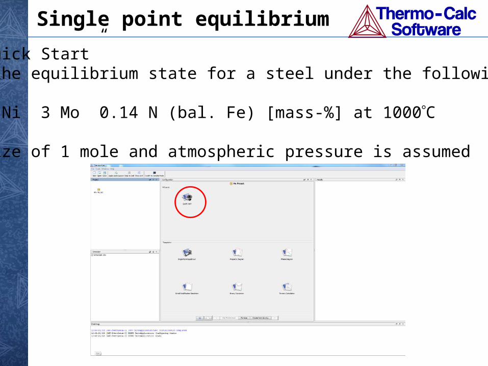
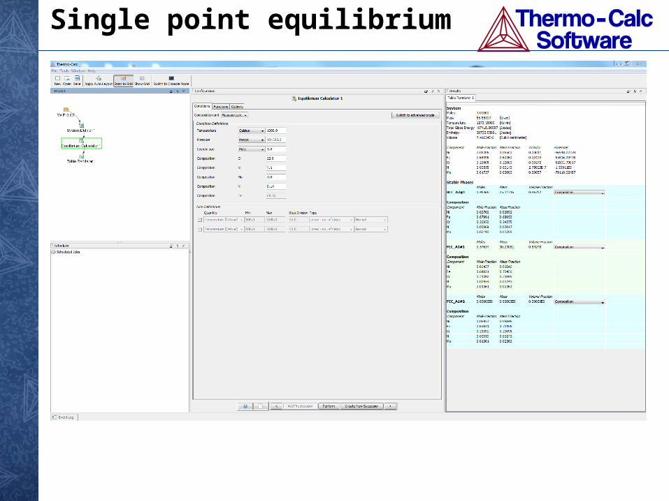
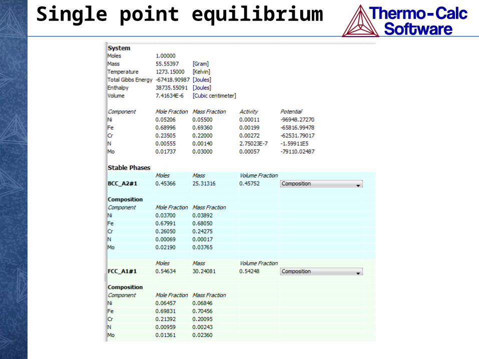
Single point equilibrium
Use the ”Quick Start”Calculate the equilibrium state for a steel under the following conditions:
22 Cr 5.5 Ni 3 Mo 0.14 N (bal. Fe) [mass-%] at 1000C
A system size of 1 mole and atmospheric pressure is assumed
Single point equilibrium
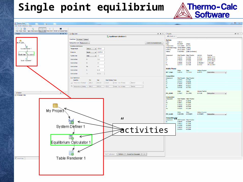
Single point equilibrium
”activities”
Single point equilibrium
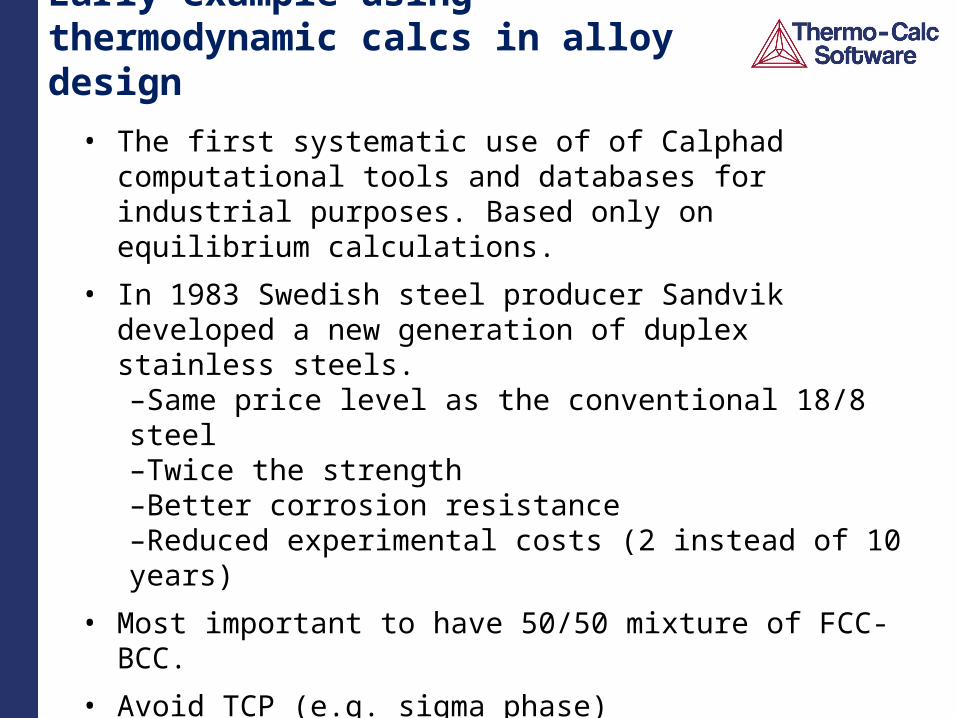
Early example using thermodynamic calcs in alloy design
• The first systematic use of of Calphad computational tools and databases for industrial purposes. Based only on equilibrium calculations.
• In 1983 Swedish steel producer Sandvik developed a new generation of duplex stainless steels. –Same price level as the conventional 18/8 steel –Twice the strength –Better corrosion resistance –Reduced experimental costs (2 instead of 10 years)
• Most important to have 50/50 mixture of FCC-BCC.
• Avoid TCP (e.g. sigma phase)
• Same PRE-number in both phases. PRE (Pitting Resistance Equivalent) calculated empirically from phase composition.
Slide courtesy of Prof. J. Ågren, KTH
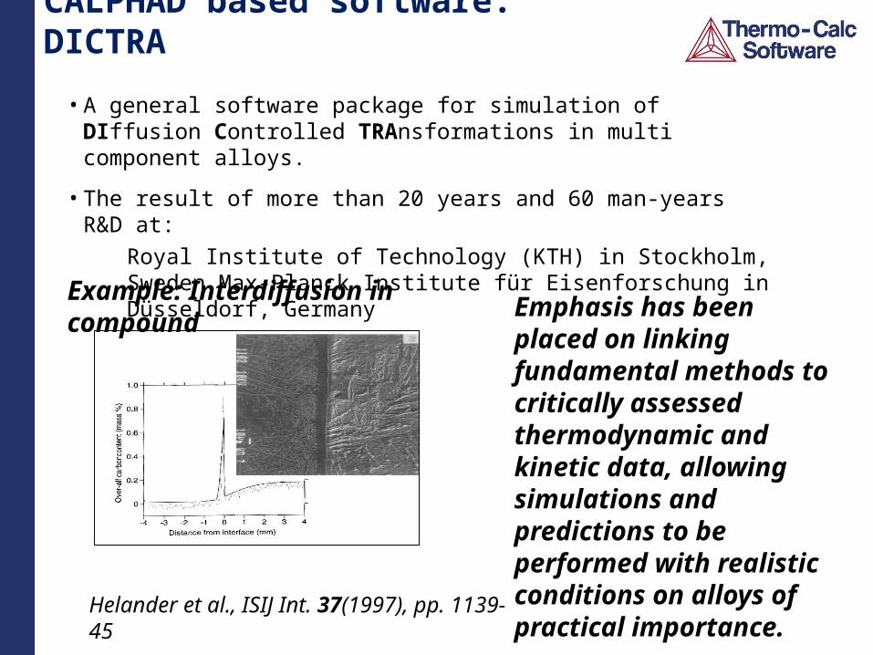
CALPHAD based software: DICTRA
• A general software package for simulation of DIffusion Controlled TRAnsformations in multi component alloys.
• The result of more than 20 years and 60 man-years R&D at: Royal Institute of Technology (KTH) in Stockholm, Sweden Max-Planck Institute für Eisenforschung in Düsseldorf, Germany
Emphasis has been placed on linking fundamental methods to critically assessed thermodynamic and kinetic data, allowing simulations and predictions to be performed with realistic conditions on alloys of practical importance.
Helander et al., ISIJ Int. 37(1997), pp. 1139-45
Example: Interdiffusion in compound
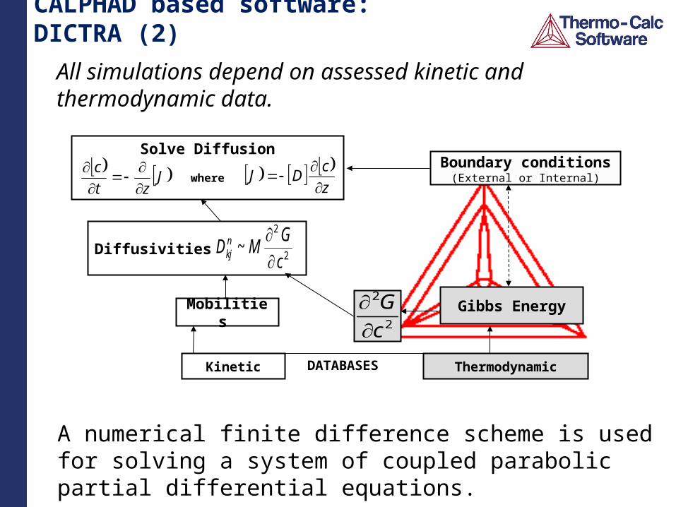
CALPHAD based software: DICTRA (2)
A numerical finite difference scheme is used for solving a system of coupled parabolic partial differential equations.
All simulations depend on assessed kinetic and thermodynamic data.
Jzt
c
DATABASESKinetic Thermodynamic
Mobilities Gibbs Energy
Diffusivities
Solve Diffusion
where
2
2
c
G
Boundary conditions(External or Internal)
z
cDJ
2
2
~c
GMDn
kj
Diffusion rates are needed
• Modelling must apply in multicomponent systems because the real alloys are multicomponent. Many diffusion coefficients!
• Various type of coupling effects may make it more complicated than Fick’s law.
• Details of geometry not of primary importance.
• An approach in the Calphad spirit was suggested for information on diffusion kinetics (Andersson-Ågren 1992)
– Allowed systematic representatation of the kinetic behaviour of multicomponent alloy systems.
• DICTRA was developed in the 1990s for numerical solution of multicomponent diffusion problems in simple geomtries.
Slide courtesy of Prof. J. Ågren, KTH
Available Kinetic Databases
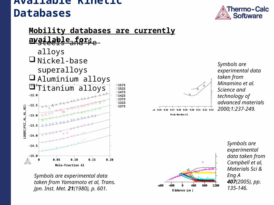
Mobility databases are currently available for: Steels and Fe-alloys Nickel-base superalloys Aluminium alloys Titanium alloys
Symbols are experimental data taken from Yamamoto et al, Trans. Jpn. Inst. Met. 21(1980), p. 601.
-15.0
-14.5
-14.0
-13.5
-13.0
-12.5
-12.0
-11.5
LO
GD
C(F
CC
,AL
,AL
,NI)
0 0.05 0.10 0.15 0.20
Mole-Fraction Al
1573 1523 1473 1423 1373 1323 1273 10
-16
10-15
10-14
10-13
10-12
D*
(B2,
Pt)
0.43 0.44 0.45 0.46 0.47 0.48 0.49 0.50 0.51 0.52 0.53
Mole fraction Al
Minamimo et al. 1423 K 1473 K 1523 K 1573 K 1623 K
1423K
1473K
1523K
1573K
1623K
Symbols are experimental data taken from Minamino et al. Science and technology of advanced materials 2000;1:237-249.
0
0.02
0.04
0.06
0.08
0.10
0.12
0.14
0.16
0.18
0.20
Mas
s F
ract
ion
-1200 -800 -400 0 400 800 1200
Distance (m)
DICTRA (2006-05-09:20.57.50) :TIME = 3600000
Al Co Cr Fe Mo Nb Ti
2006-05-09 20:57:50.12 output by user anders from NEMO
Symbols are experimental data taken from Campbell et al, Materials Sci & Eng A 407(2005), pp. 135-146.
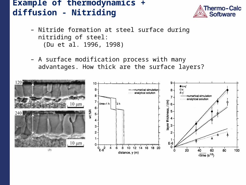
Example of thermodynamics + diffusion - Nitriding
– Nitride formation at steel surface during nitriding of steel: (Du et al. 1996, 1998)
– A surface modification process with many advantages. How thick are the surface layers?
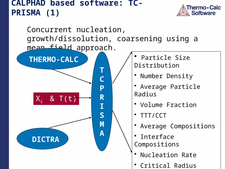
CALPHAD based software: TC-PRISMA (1)
Concurrent nucleation, growth/dissolution, coarsening using a mean field approach.
THERMO-CALC
DICTRA
TCPRISMA
• Particle Size Distribution
• Number Density
• Average Particle Radius
• Volume Fraction
• TTT/CCT
• Average Compositions
• Interface Compositions
• Nucleation Rate
• Critical Radius
Xi & T(t)
The need for interfacial energies
The length scale is typically determined by a combination of thermodynamic driving forces, interfacial energy, diffusion and the dynamic nature of the process.
Modelling and databases for interfacial energy needed.
In the simplest case interfacial energy is just a number (which may be difficult to determine experimentally but could be obtained from e.g. coarsening studies). Because of uncertainty could be treated as a calibration factor.
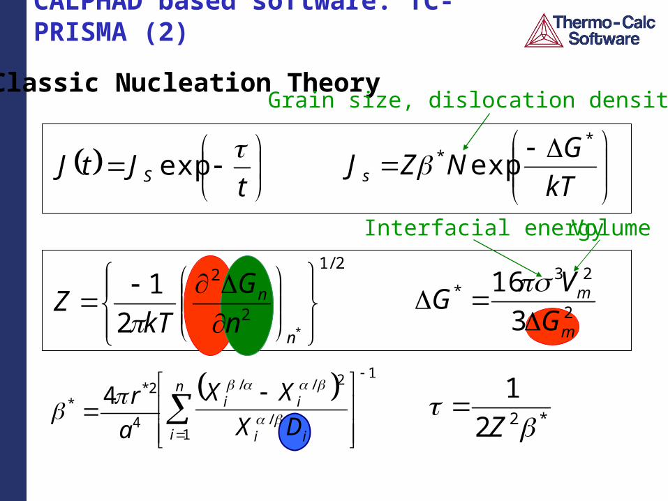
CALPHAD based software: TC-PRISMA (2)
Classic Nucleation TheoryGrain size, dislocation density, etc
kT
GNZJ s
** exp
tJtJ S
exp
2/1
2
2
*2
1
n
n
n
G
kTZ
*22
1
Z
*2*
4
4 r
a
1
1/
2//
n
i ii
ii
DX
XX
2
23*
3
16
m
m
G
VG
Interfacial energy Volume
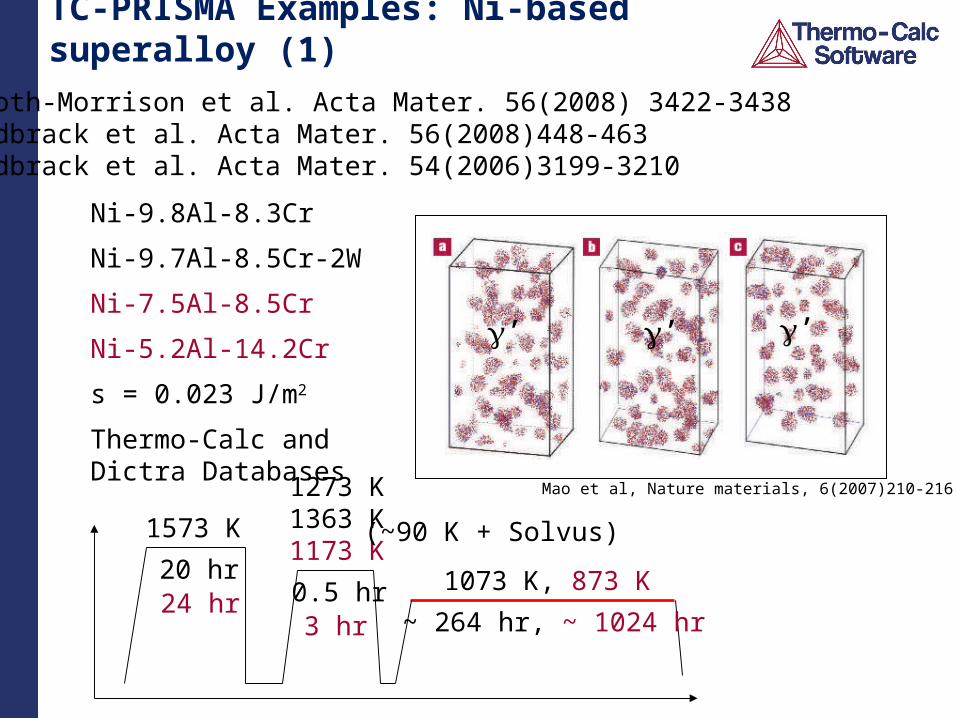
TC-PRISMA Examples: Ni-based superalloy (1)
1573 K
20 hr
1273 K1363 K1173 K
1073 K, 873 K0.5 hr~ 264 hr, ~ 1024 hr
Ni-9.8Al-8.3Cr
Ni-9.7Al-8.5Cr-2W
Ni-7.5Al-8.5Cr
Ni-5.2Al-14.2Cr
s = 0.023 J/m2
Thermo-Calc and Dictra Databases
Booth-Morrison et al. Acta Mater. 56(2008) 3422-3438Sudbrack et al. Acta Mater. 56(2008)448-463Sudbrack et al. Acta Mater. 54(2006)3199-3210
Mao et al, Nature materials, 6(2007)210-216
(~90 K + Solvus)
g’ g’ g’
24 hr3 hr
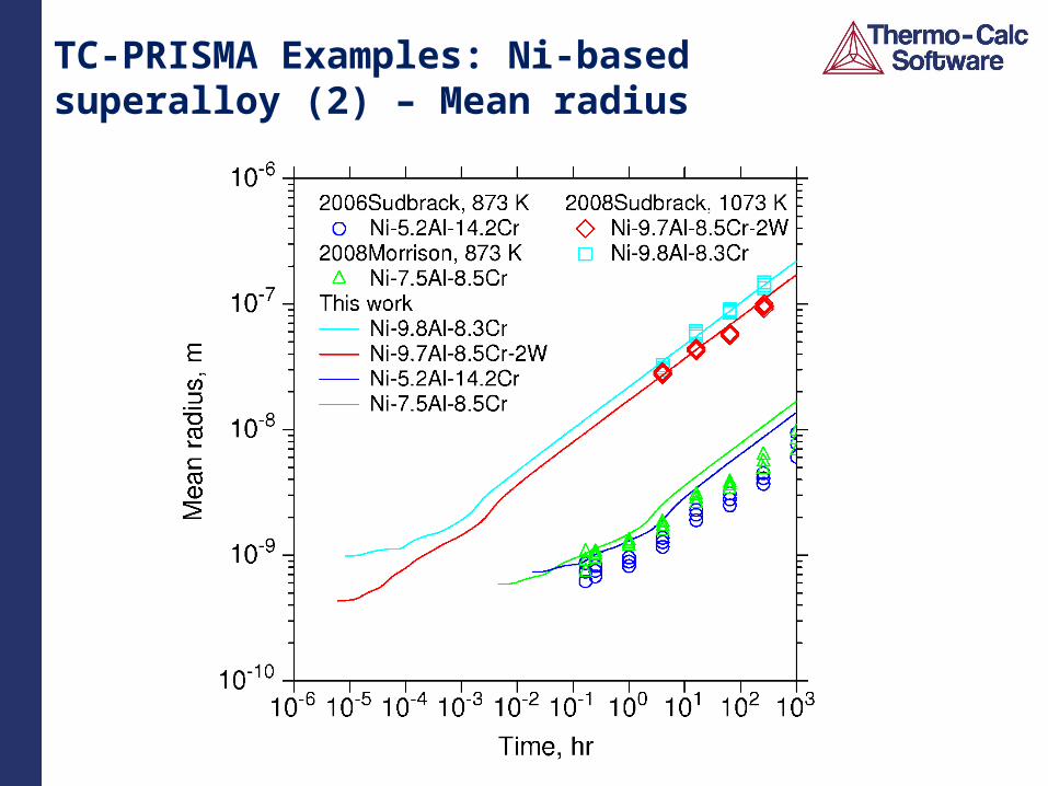
TC-PRISMA Examples: Ni-based superalloy (2) – Mean radius
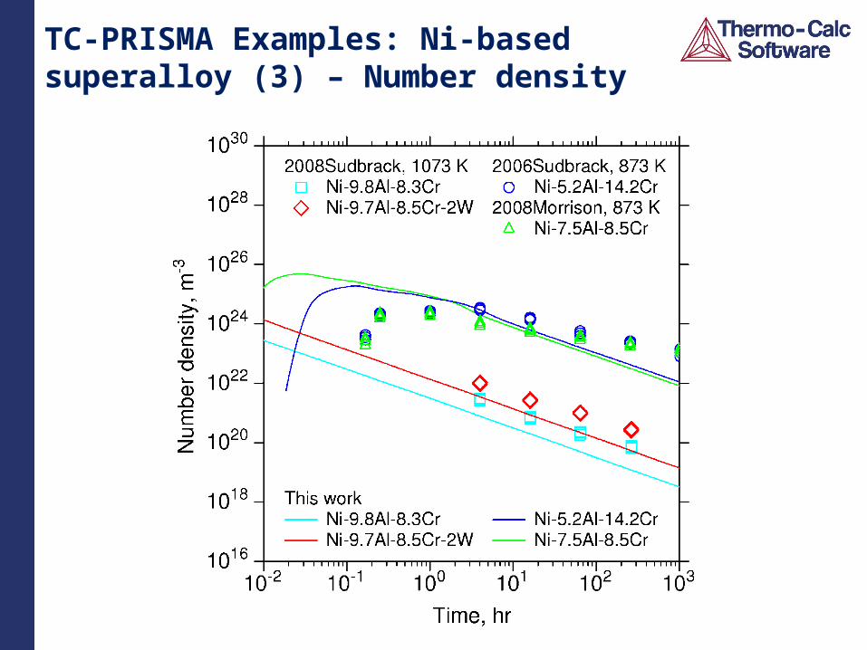
TC-PRISMA Examples: Ni-based superalloy (3) – Number density
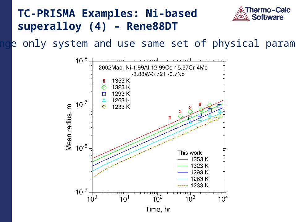
TC-PRISMA Examples: Ni-based superalloy (4) – Rene88DT
Change only system and use same set of physical parameters
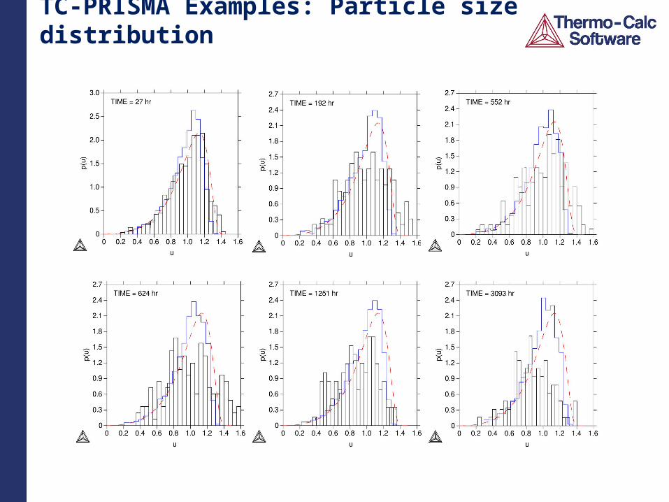
TC-PRISMA Examples: Particle size distribution
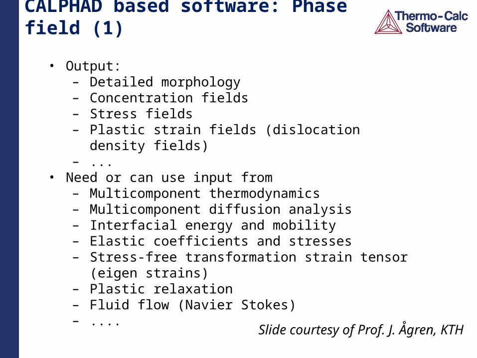
CALPHAD based software: Phase field (1)
• Output:– Detailed morphology– Concentration fields– Stress fields– Plastic strain fields (dislocation density fields)– ...
• Need or can use input from– Multicomponent thermodynamics– Multicomponent diffusion analysis– Interfacial energy and mobility– Elastic coefficients and stresses– Stress-free transformation strain tensor (eigen strains)– Plastic relaxation– Fluid flow (Navier Stokes)– ....
Slide courtesy of Prof. J. Ågren, KTH
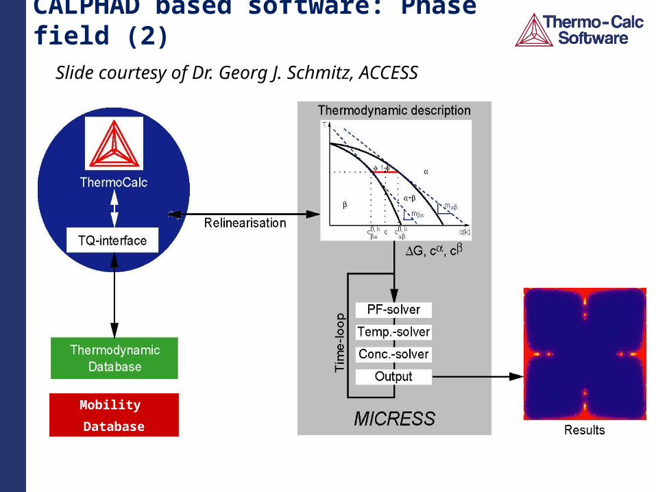
CALPHAD based software: Phase field (2)
Mobility
Database
Slide courtesy of Dr. Georg J. Schmitz, ACCESS
The underlying principles Of CALPHAD and
Thermo-Calc
Thermodynamics
ISBN 978-0-521-85351-4
Assessment guide
ISBN 978-0-521-86811
Behind Thermo-Calc
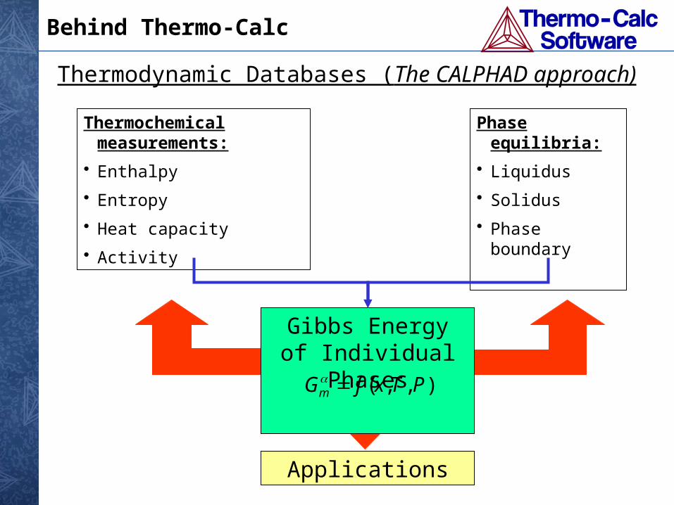
Thermodynamic Databases (The CALPHAD approach)
Thermochemical measurements:
• Enthalpy
• Entropy
• Heat capacity
• Activity
Phase equilibria:
• Liquidus
• Solidus
• Phase boundary
Gibbs Energy of Individual Phases
Applications
),,( PTxfGm
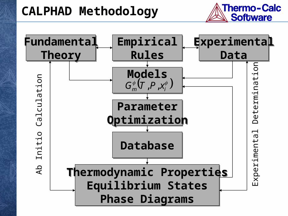
CALPHAD Methodology
FundamentalTheory
FundamentalTheory
EmpiricalRules
EmpiricalRules
ExperimentalData
ExperimentalData
ModelsModels
ParameterOptimizationParameter
Optimization
DatabaseDatabase
Thermodynamic PropertiesEquilibrium States
Phase Diagrams
Thermodynamic PropertiesEquilibrium States
Phase Diagrams
Ab
Initi
o C
alcu
latio
n
Exp
erim
enta
l Det
erm
inat
ion
im xPTG ,,
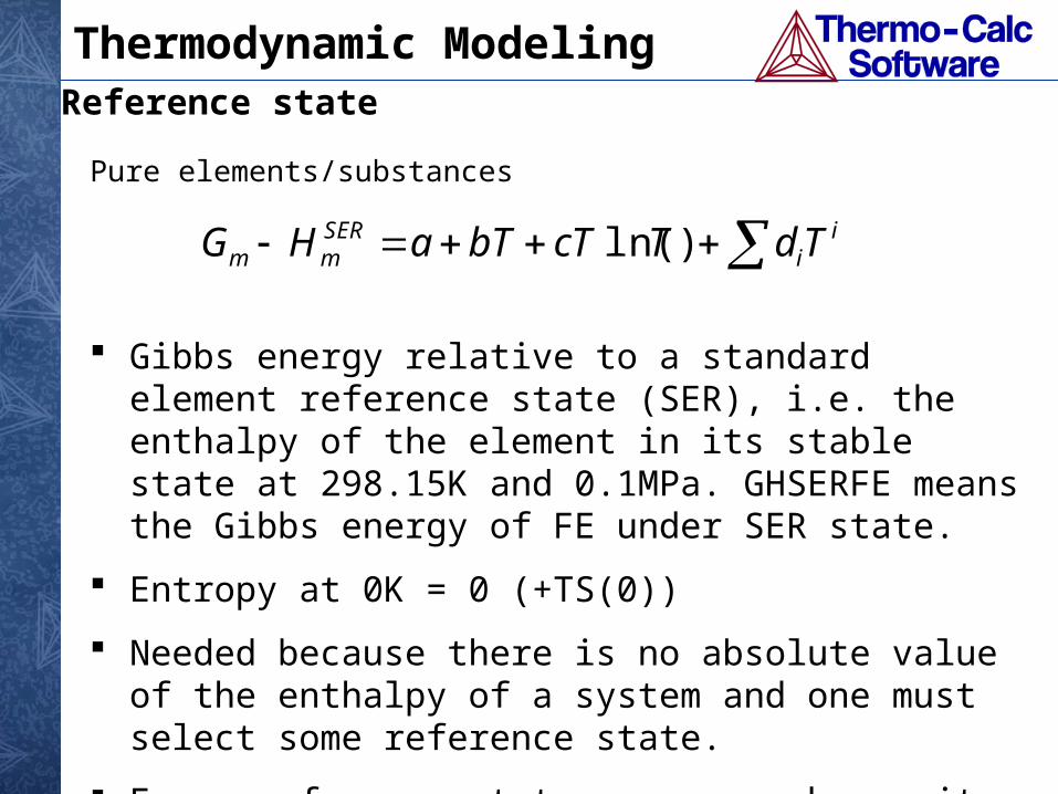
Thermodynamic Modeling
Pure elements/substances
ii
SERmm TdTcTbTaHG )ln(
Gibbs energy relative to a standard element reference state (SER), i.e. the enthalpy of the element in its stable state at 298.15K and 0.1MPa. GHSERFE means the Gibbs energy of FE under SER state.
Entropy at 0K = 0 (+TS(0))
Needed because there is no absolute value of the enthalpy of a system and one must select some reference state.
For a reference state, one can change its phase structure, temperature, and pressure.
Reference state
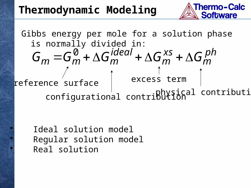
Thermodynamic Modeling
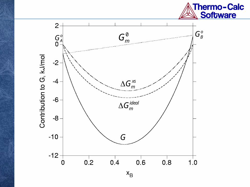
Gibbs energy per mole for a solution phase is normally divided in:
phm
xsm
idealmmm GGGGG 0
• Ideal solution model• Regular solution model• Real solution
reference surface
configurational contribution physical contribution
excess term
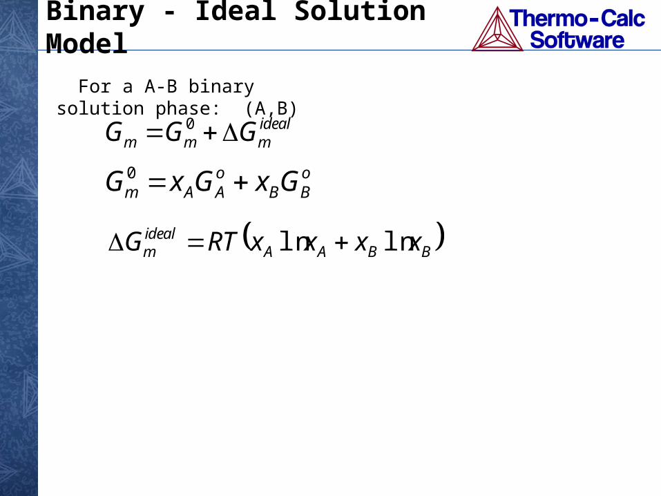
Binary - Ideal Solution Model
For a A-B binary solution phase: (A,B)
oBB
oAAm GxGxG 0
BBAAidealm xxxxRTG lnln
idealmmm GGG 0
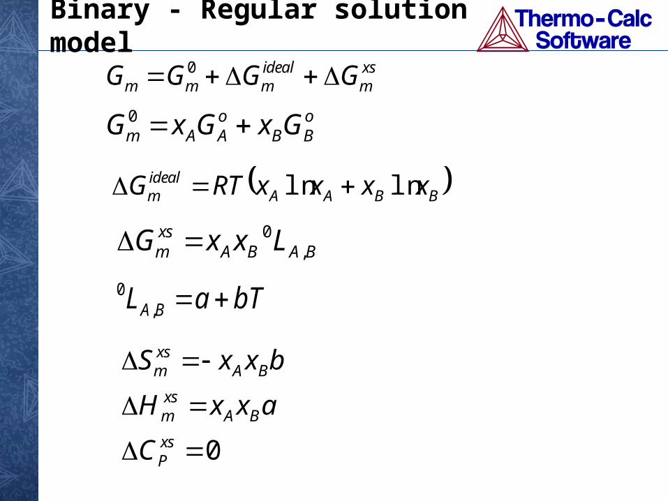
Binary - Regular solution model
bTaL BA ,0
0
xsP
BAxsm
BAxsm
C
axxH
bxxS
oBB
oAAm GxGxG 0
BBAAidealm xxxxRTG lnln
xsm
idealmmm GGGG 0
BABAxsm LxxG ,
0
oAG
oBG0
mG
idealmG
xsmG
G
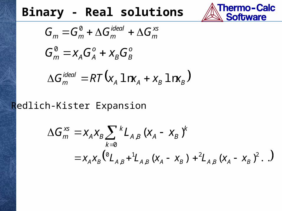
Binary - Real solutions
oBB
oAAm GxGxG 0
BBAAidealm xxxxRTG lnln
xsm
idealmmm GGGG 0
0
, )(k
kBABA
kBA
xsm xxLxxG
....)()( 2,
2,
1,
0BABABABABABA xxLxxLLxx
Redlich-Kister Expansion
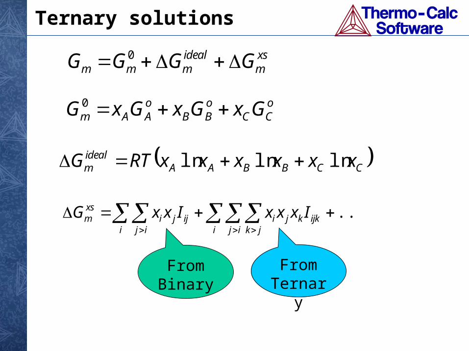
Ternary solutions
oCC
oBB
oAAm GxGxGxG 0
CCBBAAidealm xxxxxxRTG lnlnln
.... i ij jk
ijkkjii ij
ijjixsm IxxxIxxG
From Binary
From Ternary
xsm
idealmmm GGGG 0
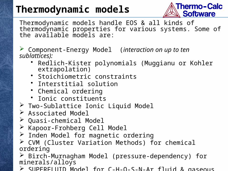
Thermodynamic models handle EOS & all kinds of thermodynamic properties for various systems. Some of the available models are:
Component-Energy Model (interaction on up to ten sublattices): • Redlich-Kister polynomials (Muggianu or Kohler extrapolation)• Stoichiometric constraints• Interstitial solution• Chemical ordering• Ionic constituents
Two-Sublattice Ionic Liquid Model Associated Model Quasi-chemical Model Kapoor-Frohberg Cell Model Inden Model for magnetic ordering CVM (Cluster Variation Methods) for chemical ordering Birch-Murnagham Model (pressure-dependency) for minerals/alloys SUPERFLUID Model for C-H-O-S-N-Ar fluid & gaseous mixtures DHLL, SIT, HKF and PITZ Models for aqueous solutions Flory-Huggins Model for polymers
Thermodynamic models
The sublattice model has been used extensively to describe interstitial solutions, carbides, oxides, intermetallic phases etc.
It is often called the compound energy formalism (CEF) as one of its features is the assumption that the compound energies are independent of composition. It includes several models as special cases.
Note that the Gm for sublattice phases is usually expressed in moles for formula units, not moles of atoms as vacancies may be constituents.
Compound Energy Formalism (CEF)
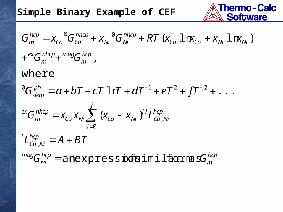
Simple Binary Example of CEF
hcpm
hcpm
mag
hcpNiCo
i
hcpNiCo
iiNi
j
iCoNiCo
nhcpm
ex
phelem
hcpm
magnhcpm
ex
NiNiCoConhcpNiNi
nhcpCoCo
hcpm
GG
BTAL
LxxxxG
fTeTdTTcTbTaG
GG
xxxxRTGxGxG
as formsimilar of expressionan
)(
...ln
where
,
)lnln(
,
,0
2210
00
Simple Binary Example of CEF
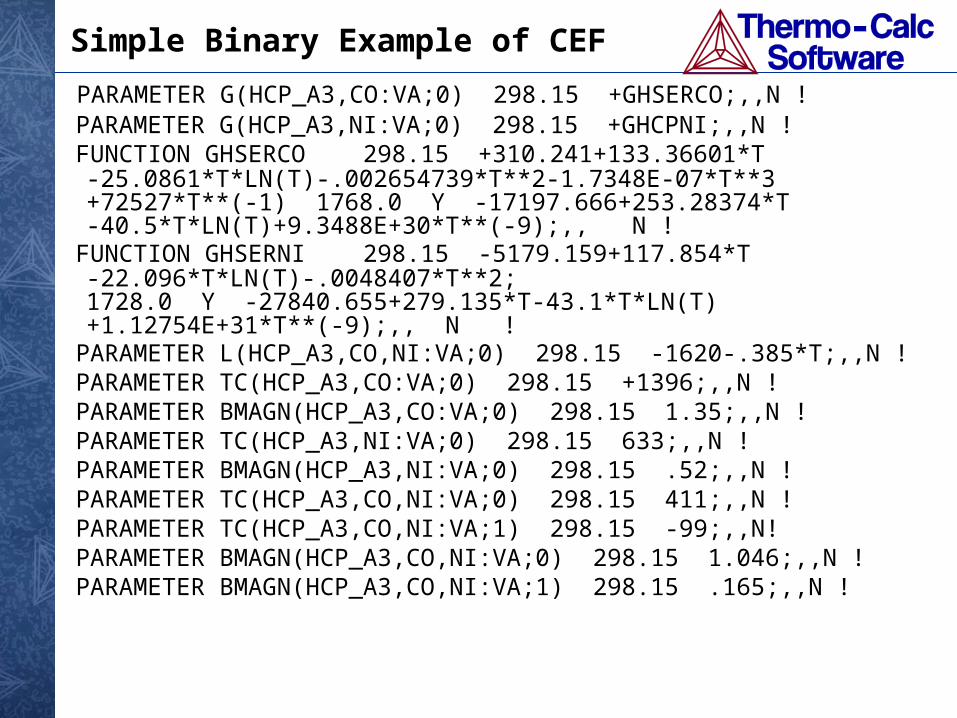
PARAMETER G(HCP_A3,CO:VA;0) 298.15 +GHSERCO;,,N ! PARAMETER G(HCP_A3,NI:VA;0) 298.15 +GHCPNI;,,N ! FUNCTION GHSERCO 298.15 +310.241+133.36601*T -25.0861*T*LN(T)-.002654739*T**2-1.7348E-07*T**3 +72527*T**(-1) 1768.0 Y -17197.666+253.28374*T -40.5*T*LN(T)+9.3488E+30*T**(-9);,, N ! FUNCTION GHSERNI 298.15 -5179.159+117.854*T -22.096*T*LN(T)-.0048407*T**2; 1728.0 Y -27840.655+279.135*T-43.1*T*LN(T) +1.12754E+31*T**(-9);,, N ! PARAMETER L(HCP_A3,CO,NI:VA;0) 298.15 -1620-.385*T;,,N ! PARAMETER TC(HCP_A3,CO:VA;0) 298.15 +1396;,,N ! PARAMETER BMAGN(HCP_A3,CO:VA;0) 298.15 1.35;,,N ! PARAMETER TC(HCP_A3,NI:VA;0) 298.15 633;,,N ! PARAMETER BMAGN(HCP_A3,NI:VA;0) 298.15 .52;,,N ! PARAMETER TC(HCP_A3,CO,NI:VA;0) 298.15 411;,,N ! PARAMETER TC(HCP_A3,CO,NI:VA;1) 298.15 -99;,,N! PARAMETER BMAGN(HCP_A3,CO,NI:VA;0) 298.15 1.046;,,N ! PARAMETER BMAGN(HCP_A3,CO,NI:VA;1) 298.15 .165;,,N !
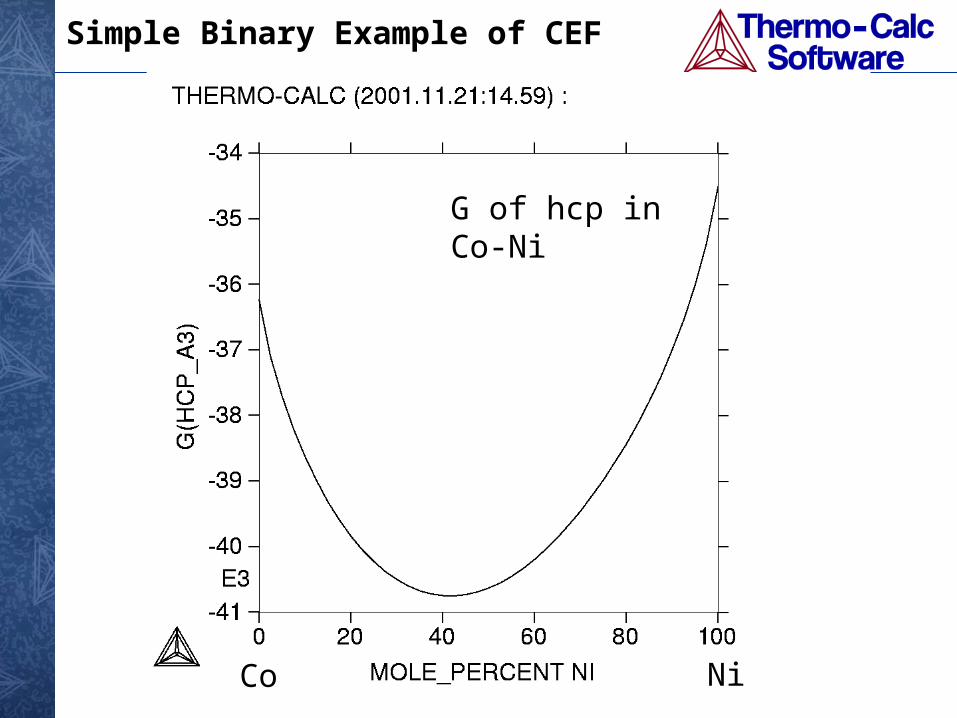
Simple Binary Example of CEF
Co Ni
G of hcp in Co-Ni
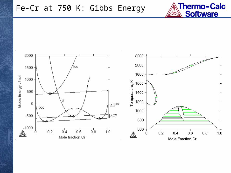
Fe-Cr at 750 K: Gibbs Energy
Thermodynamic Databases
Databases are produced by critical assessment of experimental data and optimization of model parameters (the CALPHAD method).
PARROT in Thermo-Calc Classic can be used as a tool in this process.
Description of the Gibbs energy for each phase G=G(x,T,P) is stored in the database
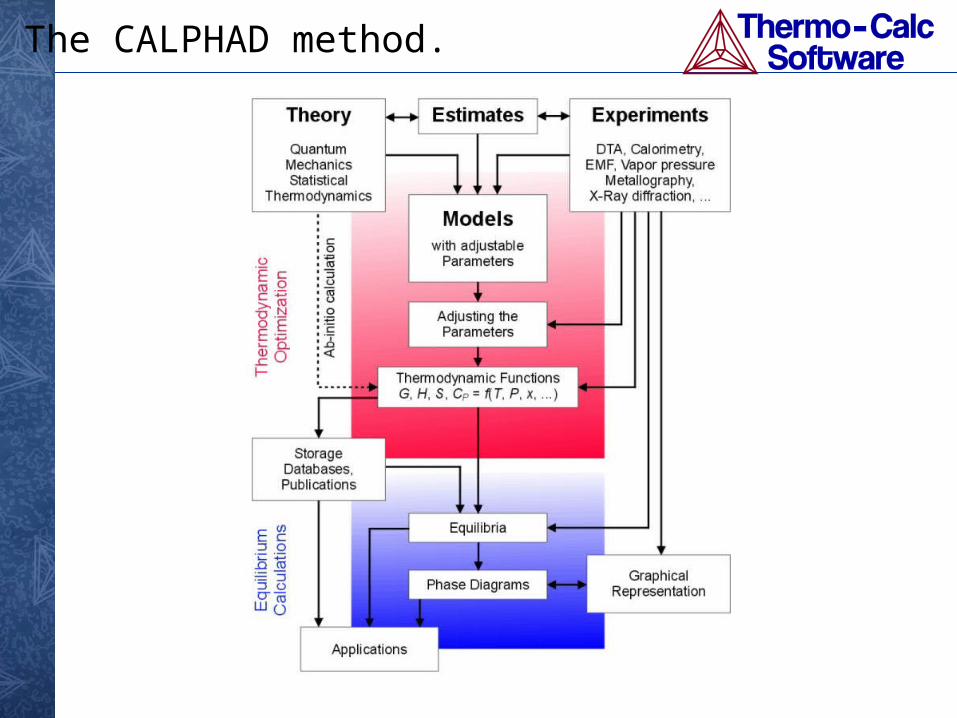
The CALPHAD method.
CALPHAD Method
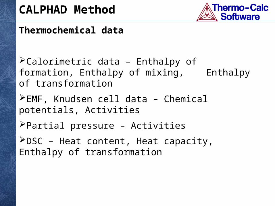
Thermochemical data
Calorimetric data – Enthalpy of formation, Enthalpy of mixing, Enthalpy of transformation
EMF, Knudsen cell data – Chemical potentials, Activities
Partial pressure – Activities
DSC – Heat content, Heat capacity, Enthalpy of transformation
CALPHAD Method
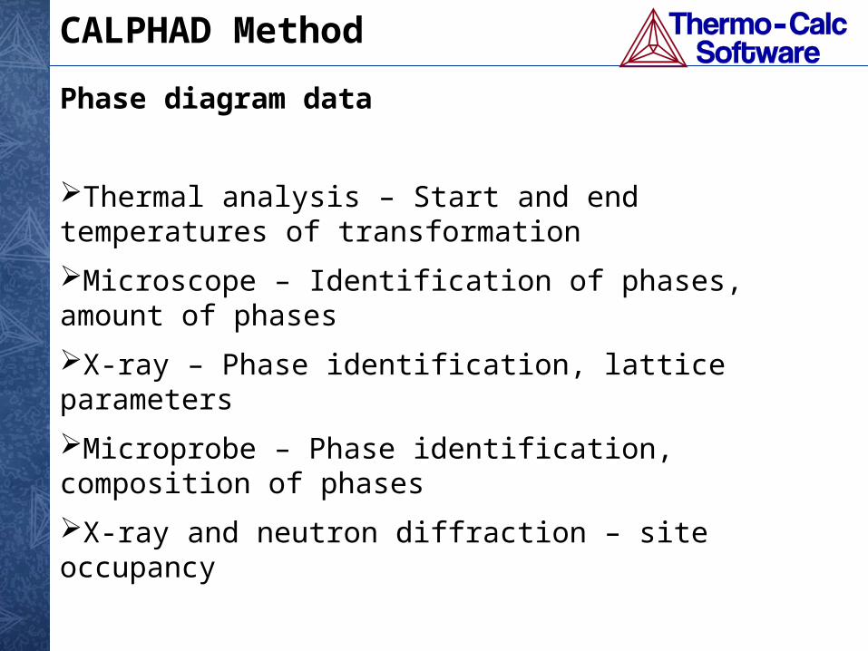
Phase diagram data
Thermal analysis – Start and end temperatures of transformation
Microscope – Identification of phases, amount of phases
X-ray – Phase identification, lattice parameters
Microprobe – Phase identification, composition of phases
X-ray and neutron diffraction – site occupancy
Sources of thermodynamic data
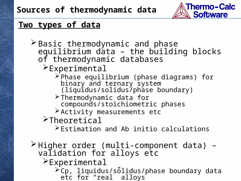
Two types of data
Basic thermodynamic and phase equilibrium data – the building blocks of thermodynamic databasesExperimental
Phase equilibrium (phase diagrams) for binary and ternary system (liquidus/solidus/phase boundary)
Thermodynamic data for compounds/stoichiometric phasesActivity measurements etc
TheoreticalEstimation and Ab initio calculations
Higher order (multi-component data) – validation for alloys etcExperimental
Cp, liquidus/solidus/phase boundary data etc for “real” alloysVolume fraction of carbides etc
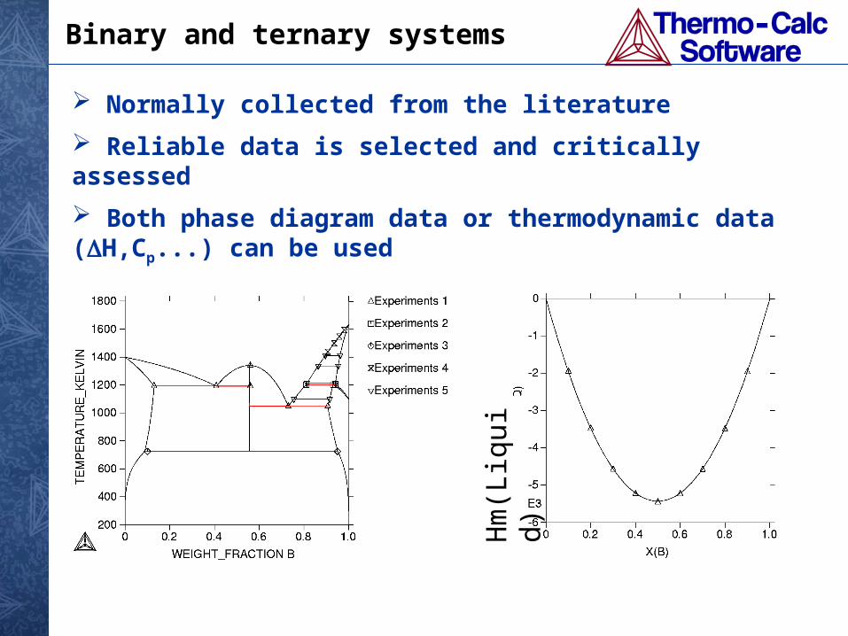
Normally collected from the literature
Reliable data is selected and critically assessed
Both phase diagram data or thermodynamic data (DH,Cp...) can be used
Hm
(Liq
uid)
Binary and ternary systems
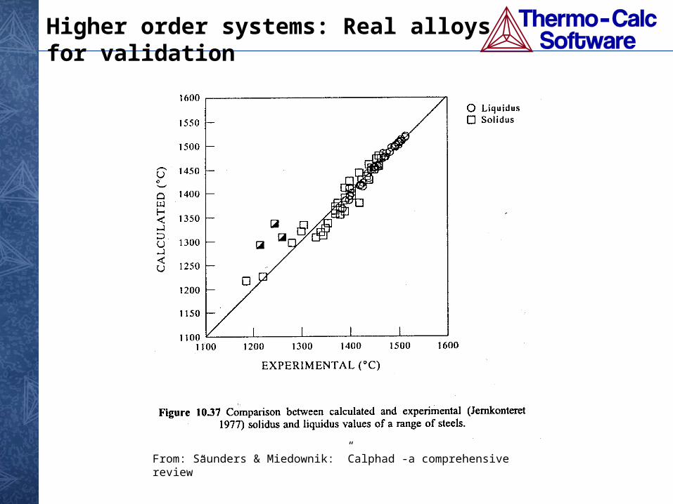
From: Saunders & Miedownik: ”Calphad -a comprehensive review”
Higher order systems: Real alloys for validation
3.50
3.52
3.54
3.56
3.58
3.60
3.62
3.64
3.66
3.68
3.70
C
alcu
late
d l
atti
ce p
aram
eter
3.50 3.55 3.60 3.65 3.70 Experimental lattice parameter
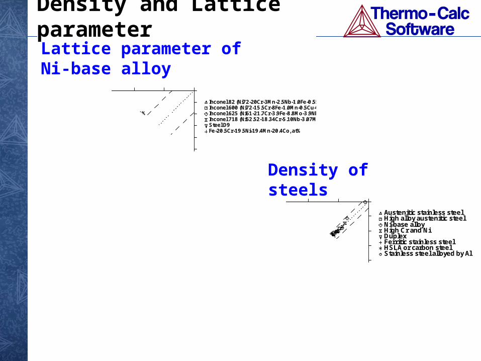
Inconel 82 (Ni72-20Cr-3Mn-2.5Nb-1.0Fe-0.55Ti-0.2Si) Inconel 600 (Ni72-15.5Cr-8Fe-1.0Mn-0.5Cu-0.5Si) Inconel 625 (Ni61-21.7Cr-3.9Fe-8.8Mo-3.9Nb-0.23Ti-0.15Si) Inconel 718 (Ni52.52-18.34Cr-5.10Nb-3.07Mo-1.0Ti-0.5Al) Steel D9 Fe-20.5Cr-19.5Ni-19.4Mn-20.4Co, at%
+1%
-1%
Lattice parameter of Ni-base alloy
6800
7000
7200
7400
7600
7800
8000
8200
8400
C
alcu
late
d d
ensi
ty (
kg/m
3)
6800 7200 7600 8000 8400 Experimental density (kg/m3)
Austenitic stainless steel High alloy austenitic steel Ni-base alloy High Cr and Ni Duplex Ferritic stainless steel HSLA or carbon steel Stainless steel alloyed by Al
-1%
+1%
Density of steels
Density and Lattice parameter
6800
6900
7000
7100
7200
7300
7400
7500
7600
7700
7800D
ensi
ty (
Kg
/m3)
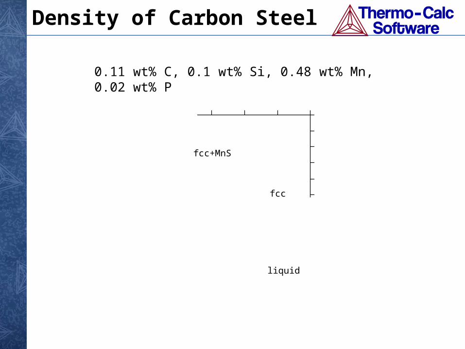
1000 1200 1400 1600 1800 2000TEMPERATURE_KELVIN
02Mizukami
0.11 wt% C, 0.1 wt% Si, 0.48 wt% Mn, 0.02 wt% P
fcc+MnS
liquid
fcc
Density of Carbon Steel
Examples of applications related to
the materials life cycle
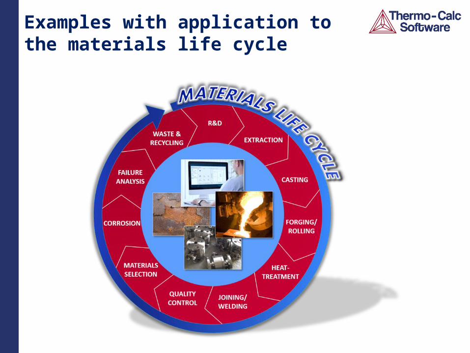
Examples with application to the materials life cycle
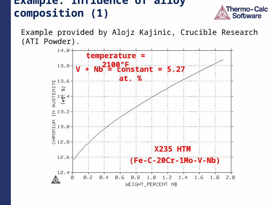
Example: Influence of alloy composition (1)
temperature = 2100°F
V + Nb = constant = 5.27 at. %(w
t. %
)
(Fe-C-20Cr-1Mo-V-Nb)
X235 HTM
Example provided by Alojz Kajinic, Crucible Research (ATI Powder).
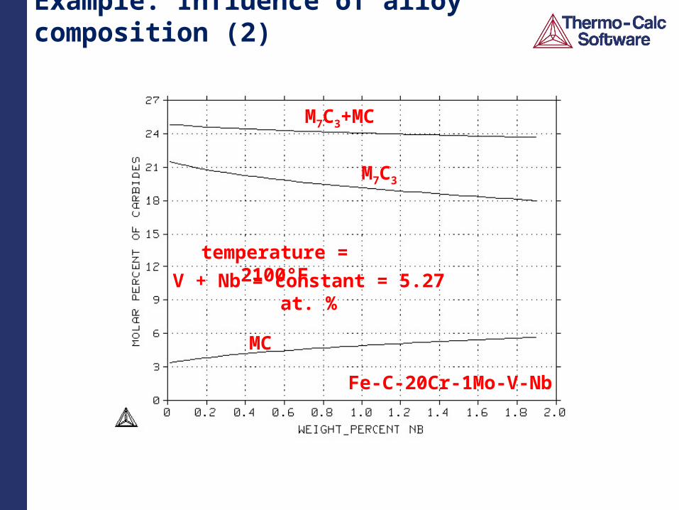
Example: Influence of alloy composition (2)
temperature = 2100°F
V + Nb = constant = 5.27 at. %
MC
M7C3
M7C3+MC
Fe-C-20Cr-1Mo-V-Nb
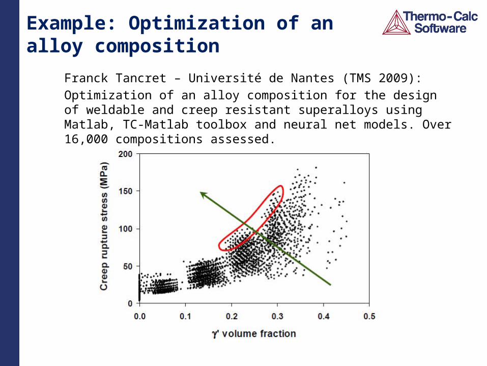
Example: Optimization of an alloy composition
Franck Tancret – Université de Nantes (TMS 2009):Optimization of an alloy composition for the design of weldable and creep resistant superalloys using Matlab, TC-Matlab toolbox and neural net models. Over 16,000 compositions assessed.
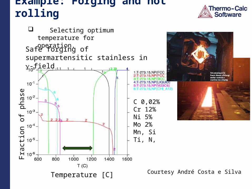
Example: Forging and hot rolling Selecting optimum
temperature for operation.
C 0,02%Cr 12%Ni 5%Mo 2%Mn, Si Ti, N,
Frac
tion
of p
hase
Temperature [C] Courtesy André Costa e Silva
Safe forging of supermartensitic stainless in -field
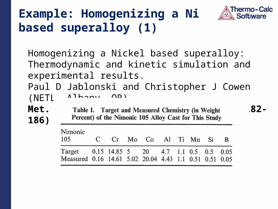
Example: Homogenizing a Ni based superalloy (1)
Homogenizing a Nickel based superalloy: Thermodynamic and kinetic simulation and experimental results. Paul D Jablonski and Christopher J Cowen (NETL, Albany, OR)Met. Trans. B. Vol 40B, April 2009 (pp 182-186)
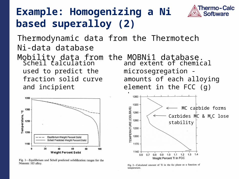
Example: Homogenizing a Ni based superalloy (2)Thermodynamic data from the Thermotech Ni-data databaseMobility data from the MOBNi1 database.
Scheil calculationused to predict the fraction solid curve and incipient melting temp -1142C.
and extent of chemical microsegregation - amounts of each alloying element in the FCC (g) phase
MC carbide forms
Carbides MC & M6C lose stability
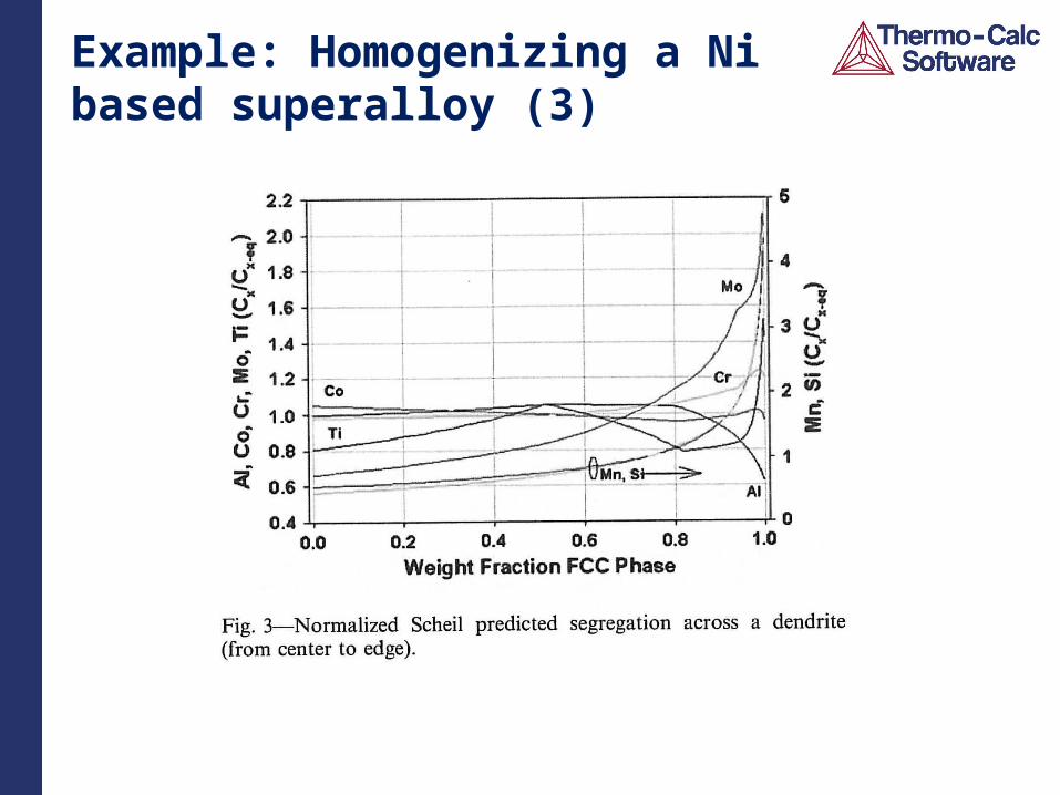
Example: Homogenizing a Ni based superalloy (3)
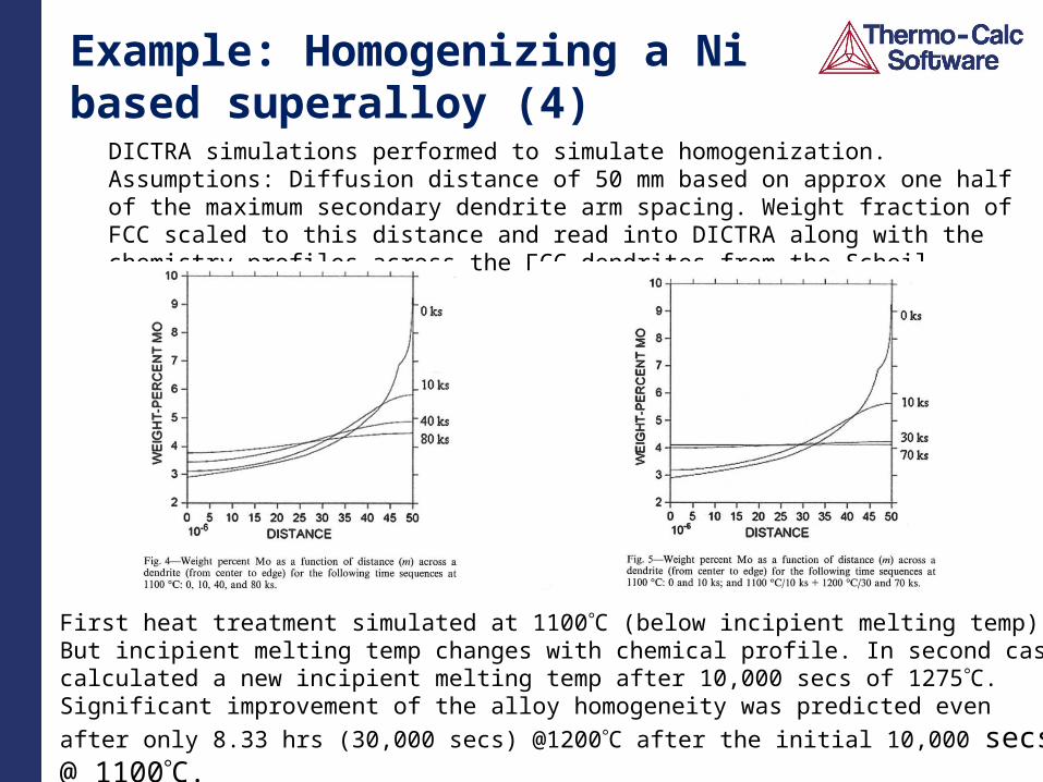
Example: Homogenizing a Ni based superalloy (4)
DICTRA simulations performed to simulate homogenization.Assumptions: Diffusion distance of 50 mm based on approx one half of the maximum secondary dendrite arm spacing. Weight fraction of FCC scaled to this distance and read into DICTRA along with the chemistry profiles across the FCC dendrites from the Scheil simulations.
First heat treatment simulated at 1100C (below incipient melting temp).But incipient melting temp changes with chemical profile. In second case calculated a new incipient melting temp after 10,000 secs of 1275C. Significant improvement of the alloy homogeneity was predicted even after only 8.33 hrs (30,000 secs) @1200C after the initial 10,000 secs @ 1100C.
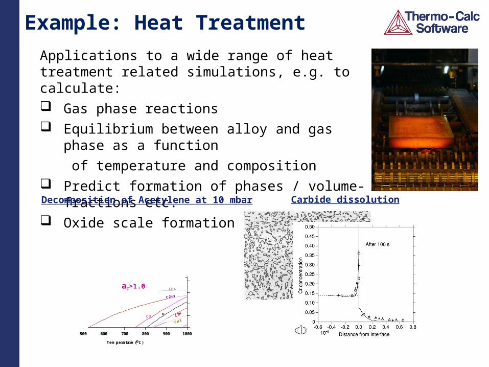
Example: Heat TreatmentApplications to a wide range of heat treatment related simulations, e.g. to calculate: Gas phase reactions Equilibrium between alloy and gas phase as a function
of temperature and composition Predict formation of phases / volume-fractions etc. Oxide scale formation
Decomposition of Acetylene at 10 mbar
10-8
10-7
10-6
10-5
10-4
.001
.01
.1
1
10
100
Part
ial
Pre
ssu
re o
f Im
po
rtan
t G
aso
ues S
pecie
s (
mb
ar)
400 500 600 700 800 900 1000
Temperature (oC)
THERMO-CALC (2006.09.15:17.53) :
H
H2
C3
CH4
C2H2
C2H4C5
Graphite suspended
Decomposition of Acetylene at 10 mbar and various temperatures
2006-09-15 17:58:52.13 output by user pingfang from PIFF
aC>1.0
Carbide dissolution
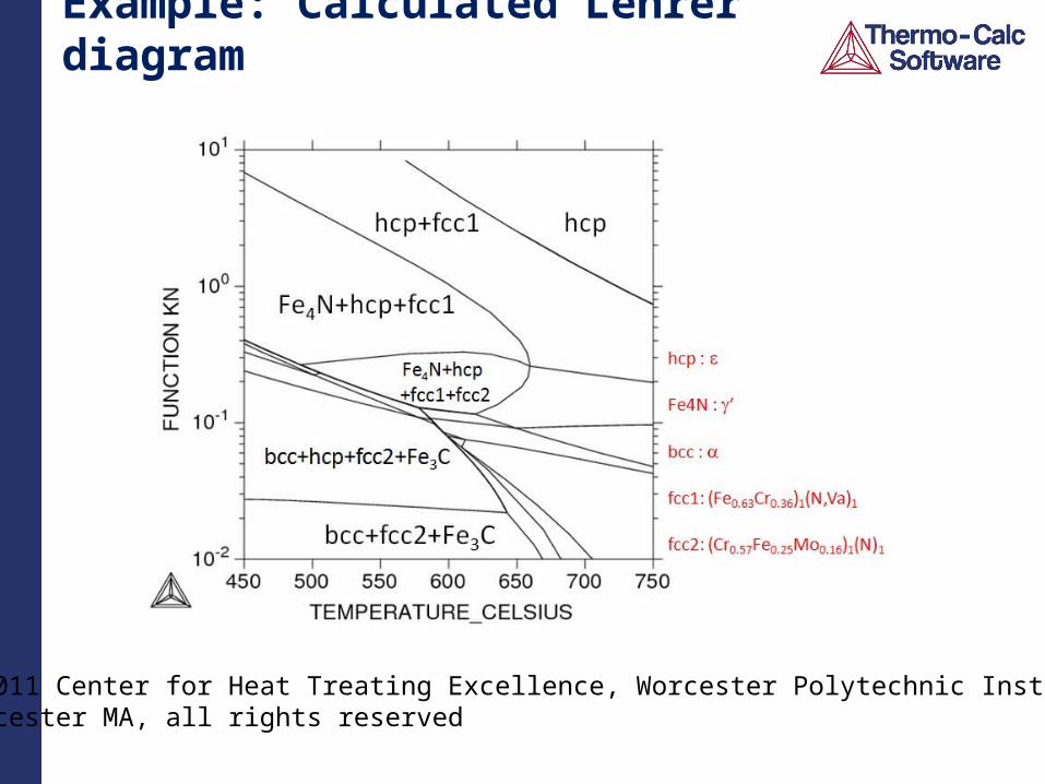
Example: Calculated Lehrer diagram
© 2011 Center for Heat Treating Excellence, Worcester Polytechnic Institute, Worcester MA, all rights reserved
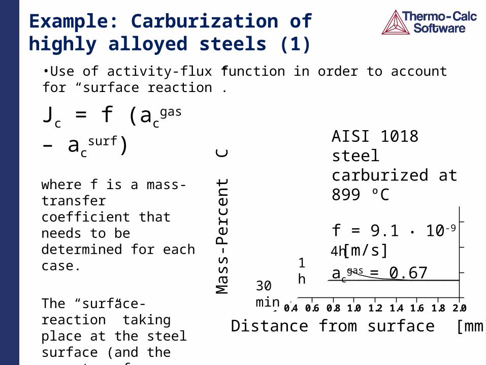
Example: Carburization of highly alloyed steels (1)
•Use of activity-flux function in order to account for “surface reaction”.
0.1
0.2
0.3
0.4
0.5
0.6
0.7
0.8
0.9
WE
IGH
T-P
ER
CE
NT
C
0.0 0.2 0.4 0.6 0.8 1.0 1.2 1.4 1.6 1.8 2.0
DISTANCE
DICTRA (2006-05-21:16.34.57) :TIME = 1800,3600,14400
CELL #1
2006-05-21 16:34:57.62 output by user anders from NEMO
Distance from surface [mm]
Mas
s-Pe
rcen
t C
4h1h
30 min
Jc = f (acgas – ac
surf)
where f is a mass-transfer coefficient that needs to be determined for each case.
The “surface-reaction” taking place at the steel surface (and the mass-transfer coefficient) is believed to be strongly affected by pressure.
AISI 1018 steel carburized at 899 ºC
f = 9.1 • 10-9 [m/s]ac
gas = 0.67
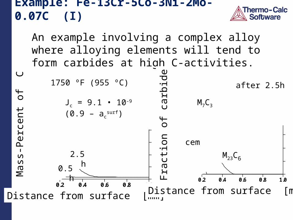
Example: Fe-13Cr-5Co-3Ni-2Mo-0.07C (I)
0
0.5
1.0
1.5
2.0
2.5
3.0
3.5
4.0
4.5
WE
IGH
T-P
ER
CE
NT
C
0.0 0.2 0.4 0.6 0.8 1.0
DISTANCE
DICTRA (2006-05-22:04.55.31) :TIME = 1800,9000
CELL #1
2006-05-22 04:55:31.57 output by user anders from NEMO
Distance from surface [mm]
Mas
s-Pe
rcen
t of
C
2.5h
0.5h
1750 ºF (955 ºC)
Jc = 9.1 • 10-9 (0.9 – acsurf)
An example involving a complex alloy where alloying elements will tend to form carbides at high C-activities.
0
0.05
0.10
0.15
0.20
0.25
0.30
0.35
0.40
TA
BL
E F
OO
0.0 0.2 0.4 0.6 0.8 1.0
DISTANCE
DICTRA (2006-05-22:05.09.17) :TIME = 9000
CELL #1
2006-05-22 05:09:17.54 output by user anders from NEMO
Distance from surface [mm]
Frac
tion
of c
arbi
deM23C6
M7C3
cem
after 2.5h
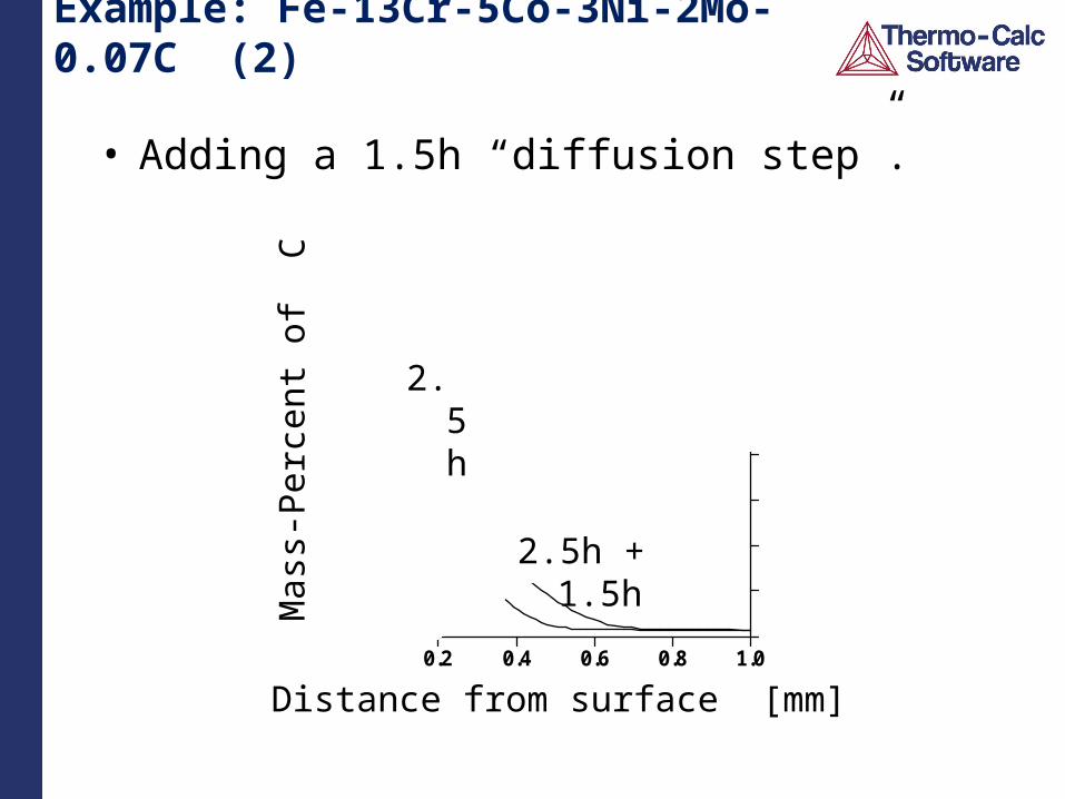
Example: Fe-13Cr-5Co-3Ni-2Mo-0.07C (2)
• Adding a 1.5h “diffusion step”.
0
0.5
1.0
1.5
2.0
2.5
3.0
3.5
4.0
4.5
WE
IGH
T-P
ER
CE
NT
C
0.0 0.2 0.4 0.6 0.8 1.0
DISTANCE
DICTRA (2006-05-22:05.16.35) :TIME = 9000,16200
CELL #1
2006-05-22 05:16:35.40 output by user anders from NEMO
Distance from surface [mm]
Mas
s-Pe
rcen
t of
C
2.5h
2.5h + 1.5h
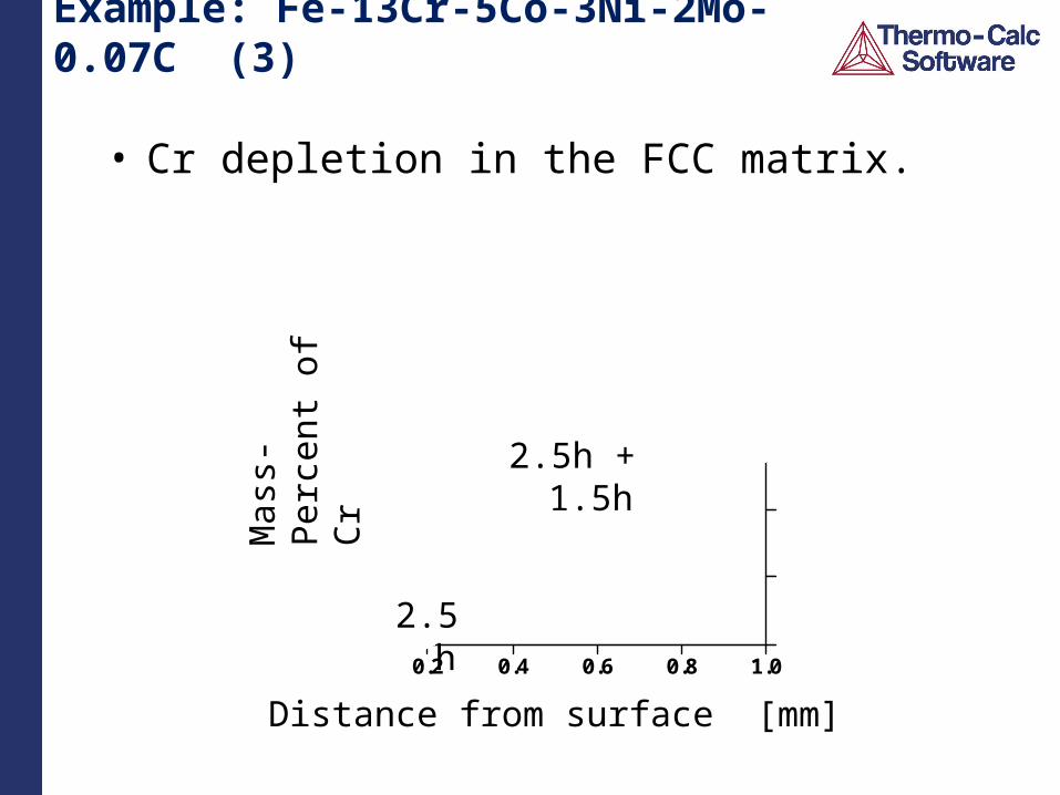
Example: Fe-13Cr-5Co-3Ni-2Mo-0.07C (3)
• Cr depletion in the FCC matrix.
0.02
0.04
0.06
0.08
0.10
0.12
0.14
W(F
CC
,CR
)
0.0 0.2 0.4 0.6 0.8 1.0
DISTANCE
DICTRA (2006-05-22:05.16.09) :TIME = 9000,16200
CELL #1
2006-05-22 05:16:09.01 output by user anders from NEMO
Distance from surface [mm]
Mas
s-Pe
rcen
t of
Cr
2.5h
2.5h + 1.5h
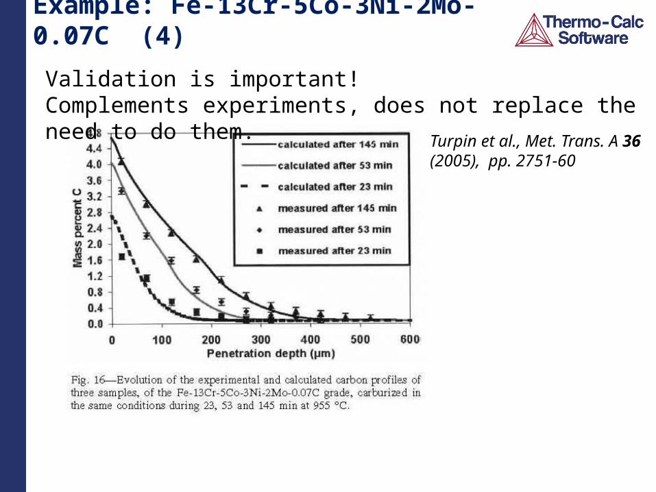
Example: Fe-13Cr-5Co-3Ni-2Mo-0.07C (4)
Turpin et al., Met. Trans. A 36 (2005), pp. 2751-60
Validation is important! Complements experiments, does not replace the need to do them.
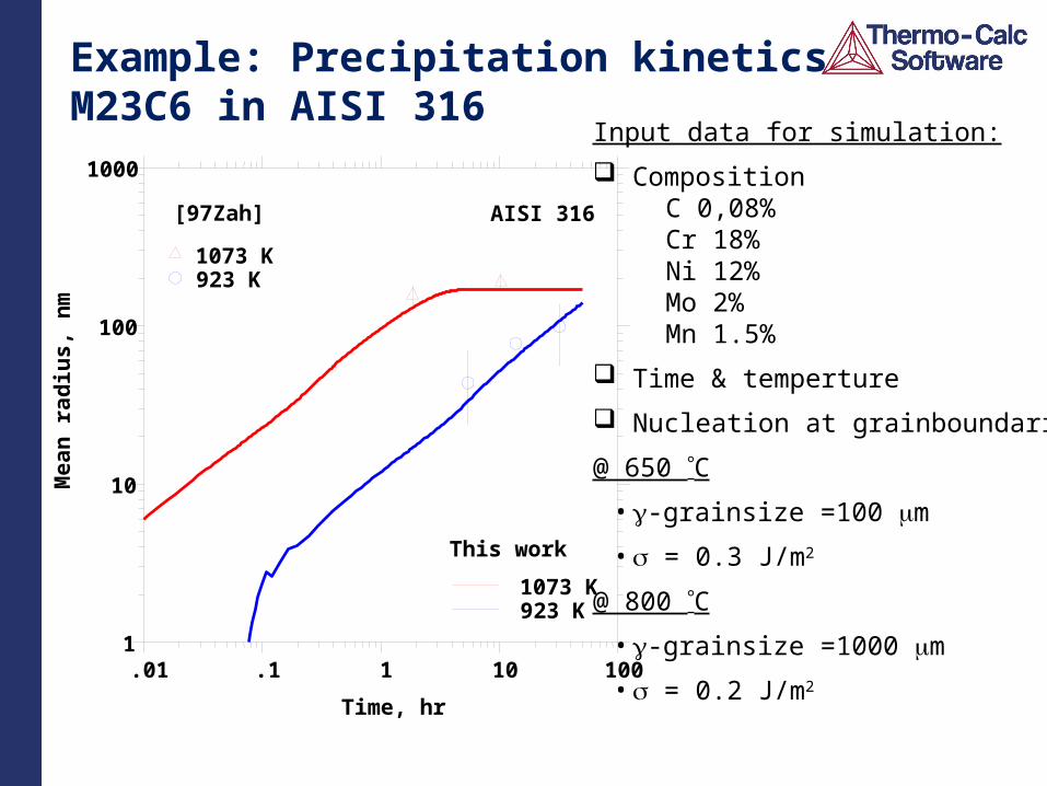
Example: Precipitation kinetics M23C6 in AISI 316
1
10
100
1000
Me
an
ra
diu
s,
nm
.01 .1 1 10 100
Time, hr
AISI 316[97Zah]
1073 K 923 K
This work
1073 K 923 K
Input data for simulation:
CompositionC 0,08%Cr 18%Ni 12%Mo 2%Mn 1.5%
Time & temperture
Nucleation at grainboundaries
@ 650 C
• -grainsize =100 m
• s = 0.3 J/m2
@ 800 C
• -grainsize =1000 m
• s = 0.2 J/m2
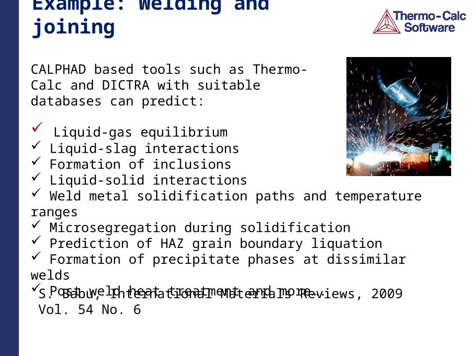
Example: Welding and joining
Liquid-gas equilibrium Liquid-slag interactions Formation of inclusions Liquid-solid interactions Weld metal solidification paths and temperature ranges Microsegregation during solidification Prediction of HAZ grain boundary liquation Formation of precipitate phases at dissimilar welds Post weld heat treatment and more….
CALPHAD based tools such as Thermo-Calc and DICTRA with suitable databases can predict:
S. Babu, International Materials Reviews, 2009 Vol. 54 No. 6
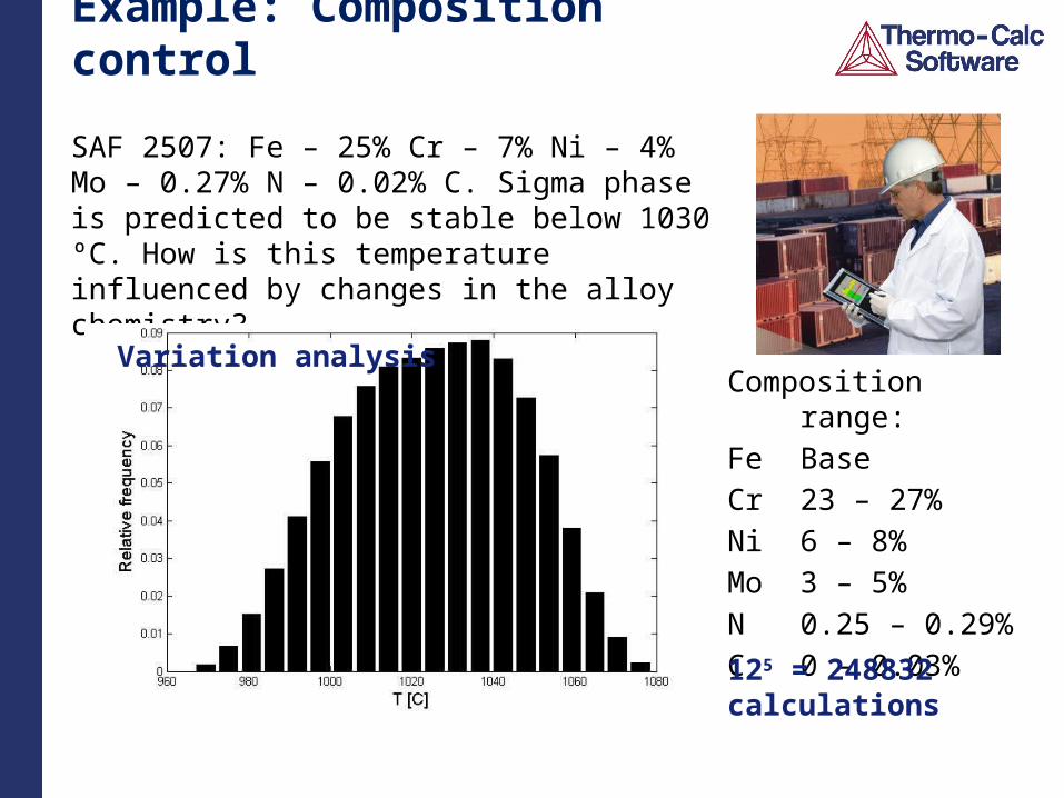
Example: Composition control
Composition range:Fe BaseCr 23 – 27%Ni 6 – 8%Mo 3 – 5%N 0.25 – 0.29%C 0 – 0.03%
SAF 2507: Fe – 25% Cr – 7% Ni – 4% Mo – 0.27% N – 0.02% C. Sigma phase is predicted to be stable below 1030 ºC. How is this temperature influenced by changes in the alloy chemistry?
125 = 248832 calculations
Variation analysis
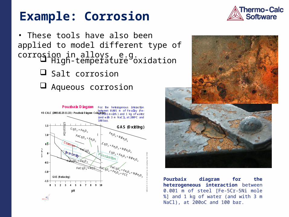
Example: Corrosion• These tools have also been applied to model different type of corrosion in alloys, e.g.
High-temperature oxidation Salt corrosion Aqueous corrosion
-1.5
-1.0
-0.5
0
0.5
1.0
1.5
Eh
(V)
0 1 2 3 4 5 6 7 8 9 10
pH
THERMO-CALC (2003.02.25:11.33) : Pourbaix Diagram Calculation
GAS (Reducing)
2003
-02-
25 1
1:57
:41.
56 o
utpu
t by
use
r pi
ngfa
ng f
rom
VITA
NI
FeCr2O4
GAS (Oxiding)
AQ
UE
OU
S
Cr2O3 + Fe2O3
Cr2O3 + Fe2O3 + NiFe
2O4Cr2O3 + Fe2O3 + NiFe
2O4
Fe2O
3 + NiFe2O
4
FeCr2O4 + Fe
3O4 + NiFe2O4
FeCr2O4 + Fe
3O4 + FCC
FeCr2O4 + FCC
FeCr2O4 + Fe2O3
FeCr2O4 + Fe3O4
Corrosion
Immunity Passivation
Pourbaix Diagram For the heterogenous interaction between 0.001 m of Fe-alloy (Fe-5Cr-5Ni mole%) and 1 kg of water (and with 3 m NaCl), at 200oC and 100 bar.
-1.2
-0.9
-0.6
-0.3
0
0.3
0.6
0.9
1.2
Eh (V
)
0 2 4 6 8 10 12 14
pH
THERMO-CALC (2003.11.26): Pourbaix Diagram Calculation
T=358.15 K, P=1 bar, B(H2O)=1000 g, N(H2SO4)=0.537 mN(Fe)=1.2266E-3, N(Cr)=3.2695E-4, N(M o)=2.6058E-5, N(Ni)=2.0446E-4
1:*CR2O3 2:*HEMATITE
3:*MOO2 4:*FECR2O4
5:*MOS2
5
3
2
51
6:*MAGNETITE
6
2
7
7:*PYRITE
4
8:*NIS2
8
8
71
9:*GAS
4
4
9
10:*AQUEOUS
11:*PYRRHOTITE_FE_877S
11
1110
12:*NI3S2
12
7
13:*NIS
1211
1112
13
1
8
8
8
7 1
9
9
8
3
1
7
6
22
6
5
5
9
1
3
314
14:*MOO2_75 15:*MOO2_87515
16
16:*MOO2_889 17:*MOO3
17
17
2
9
91
4
13 9
13
1
4
1
2003
-11-
26 1
2:29
:31.
64 o
utpu
t by
use
r pi
ngfa
ng f
rom
PIFF
Steel: Fe- 17.00Cr-12.00Ni-2.5Mo (wt% )Aqueous Solution: 1 kg of water with 0.537 m H2SO4T=85oC, P=1 bar
-1.5
-1.0
-0.5
0
0.5
1.0
1.5
Eh
(V)
0 1 2 3 4 5 6 7 8 9 10
pH
THERMO-CALC (2003.02.25:11.33) : Pourbaix Diagram Calculation
GAS (Reducing)
2003
-02-
25 1
1:57
:41.
56 o
utpu
t by
use
r pi
ngfa
ng f
rom
VITA
NI
FeCr2O4
GAS (Oxiding)
AQ
UE
OU
S
Cr2O3 + Fe2O3
Cr2O3 + Fe2O3 + NiFe
2O4Cr2O3 + Fe2O3 + NiFe
2O4
Fe2O
3 + NiFe2O
4
FeCr2O4 + Fe
3O4 + NiFe2O4
FeCr2O4 + Fe
3O4 + FCC
FeCr2O4 + FCC
FeCr2O4 + Fe2O3
FeCr2O4 + Fe3O4
Corrosion
Immunity Passivation
Pourbaix Diagram For the heterogenous interaction between 0.001 m of Fe-alloy (Fe-5Cr-5Ni mole%) and 1 kg of water (and with 3 m NaCl), at 200oC and 100 bar.
-1.5
-1.0
-0.5
0
0.5
1.0
1.5
Eh
(V)
0 1 2 3 4 5 6 7 8 9 10
pH
THERMO-CALC (2003.02.25:11.33) : Pourbaix Diagram Calculation
GAS (Reducing)
2003
-02-
25 1
1:57
:41.
56 o
utpu
t by
use
r pi
ngfa
ng f
rom
VITA
NI
-1.5
-1.0
-0.5
0
0.5
1.0
1.5
Eh
(V)
0 1 2 3 4 5 6 7 8 9 10
pH
THERMO-CALC (2003.02.25:11.33) : Pourbaix Diagram Calculation
GAS (Reducing)
2003
-02-
25 1
1:57
:41.
56 o
utpu
t by
use
r pi
ngfa
ng f
rom
VITA
NI
FeCr2O4
GAS (Oxiding)
AQ
UE
OU
S
Cr2O3 + Fe2O3
Cr2O3 + Fe2O3 + NiFe
2O4Cr2O3 + Fe2O3 + NiFe
2O4
Fe2O
3 + NiFe2O
4
FeCr2O4 + Fe
3O4 + NiFe2O4
FeCr2O4 + Fe
3O4 + FCC
FeCr2O4 + FCC
FeCr2O4 + Fe2O3
FeCr2O4 + Fe3O4
Corrosion
Immunity Passivation
Pourbaix Diagram For the heterogenous interaction between 0.001 m of Fe-alloy (Fe-5Cr-5Ni mole%) and 1 kg of water (and with 3 m NaCl), at 200oC and 100 bar.
-1.2
-0.9
-0.6
-0.3
0
0.3
0.6
0.9
1.2
Eh (V
)
0 2 4 6 8 10 12 14
pH
THERMO-CALC (2003.11.26): Pourbaix Diagram Calculation
T=358.15 K, P=1 bar, B(H2O)=1000 g, N(H2SO4)=0.537 mN(Fe)=1.2266E-3, N(Cr)=3.2695E-4, N(M o)=2.6058E-5, N(Ni)=2.0446E-4
1:*CR2O3 2:*HEMATITE
3:*MOO2 4:*FECR2O4
5:*MOS2
5
3
2
51
6:*MAGNETITE
6
2
7
7:*PYRITE
4
8:*NIS2
8
8
71
9:*GAS
4
4
9
10:*AQUEOUS
11:*PYRRHOTITE_FE_877S
11
1110
12:*NI3S2
12
7
13:*NIS
1211
1112
13
1
8
8
8
7 1
9
9
8
3
1
7
6
22
6
5
5
9
1
3
314
14:*MOO2_75 15:*MOO2_87515
16
16:*MOO2_889 17:*MOO3
17
17
2
9
91
4
13 9
13
1
4
1
2003
-11-
26 1
2:29
:31.
64 o
utpu
t by
use
r pi
ngfa
ng f
rom
PIFF
Steel: Fe- 17.00Cr-12.00Ni-2.5Mo (wt% )Aqueous Solution: 1 kg of water with 0.537 m H2SO4T=85oC, P=1 bar
Pourbaix diagram for the heterogeneous interaction between 0.001 m of steel [Fe-5Cr-5Ni mole%] and 1 kg of water (and with 3 m NaCl), at 200oC and 100 bar.
SummaryAn important part of ICME and the MGI is aimed at improving our ability to model how processes produce material structures, how those structures give rise to material properties, and how to select materials for a given application in order to design and make better materials cheaper and faster. This requires multiscale materials models to capture the process-structures-properties-performance of a material.
CALPHAD is a phase based approach to modeling the underlying thermodynamics and phase equilibria of a system through a self consistent framework that allows extrapolation to multicomponent systems. The approach has also been extended to consider multicomponent diffusion as well. CALPHAD provides an important foundation to ICME and the MGI in a framework that is scalable to multicomponent systems of interest to industry.
For more than 20 years CALPHAD based tools have been used to accelerate alloy design and improve processes with applications throughout the materials life cycle.

Questions?


![Catalog Icme Ecab[1]](https://img.pdfslide.us/doc/110x75/544c3a1caf7959a4438b59fd/catalog-icme-ecab1.jpg)