Embed Size (px)
Citation preview
i
The ABARES/NCAP agristaples CGE model
Illustrative results for India Sally Thorpe, Caroline Gunning-Trant, Edwina Heyhoe, Patrick
Hamshere and Jammie Penm
Research by the Australian Bureau of Agricultural
and Resource Economics and Sciences
Report to client prepared for DFAT Public Sector Linkages Program
April 2014

ii
© Commonwealth of Australia Ownership of intellectual property rights Unless otherwise noted, copyright (and any other intellectual property rights, if any) in this publication is owned by the Commonwealth of Australia (referred to as the Commonwealth). Creative Commons licence All material in this publication is licensed under a Creative Commons Attribution 3.0 Australia Licence, save for content supplied by third parties, logos and the Commonwealth Coat of Arms.
Creative Commons Attribution 3.0 Australia Licence is a standard form licence agreement that allows you to copy, distribute, transmit and adapt this publication provided you attribute the work. A summary of the licence terms is available from creativecommons.org/licenses/by/3.0/au/deed.en. The full licence terms are available from creativecommons.org/licenses/by/3.0/au/legalcode. This publication (and any material sourced from it) should be attributed as: Thorpe, S, Gunning-Trant, C, Heyhoe, E, Hamshere, P & Penm, J 2014, The ABARES/NCAP agristaples CGE model–Illustrative results for India, ABARES (Report to client prepared for the DFAT Public Sector Linkages Program, Canberra, April. CC BY 3.0. Cataloguing data Thorpe, S, Gunning-Trant, C, Heyhoe, E, Hamshere, P & Penm, J 2014, The ABARES/NCAP agristaples CGE model–Illustrative results for India, ABARES (Report to client prepared for DFAT Public Sector Linkages Program), Canberra, April. ABARES project: 43215 Internet The ABARES/NCAP agristaples CGE model–Illustrative results for India is available at: daff.gov.au/abares/publications. Department of Agriculture Australian Bureau of Agricultural and Resource Economics and Sciences (ABARES) Postal address GPO Box 1563 Canberra ACT 2601 Switchboard +61 2 6272 2010| Facsimile +61 2 6272 2001 Email [email protected] Web daff.gov.au/abares Inquiries regarding the licence and any use of this document should be sent to: [email protected]. The Australian Government acting through the Department of Agriculture has exercised due care and skill in the preparation and compilation of the information and data in this publication. Notwithstanding, the Department of Agriculture, its employees and advisers disclaim all liability, including liability for negligence, for any loss, damage, injury, expense or cost incurred by any person as a result of accessing, using or relying upon any of the information or data in this publication to the maximum extent permitted by law. Acknowledgements This project was funded by the DFAT Public Sector Linkages Program. Apart from the authors of this report, many people contributed to this project whose efforts are gratefully acknowledged. Formerly of ABARES, these include Neil Andrews, Verity Linehan and Daniel Pambudi. From NCAP, these include Professor Ramesh Chand, Dr. Rajni Jain, Dr. Raka Saxena and Dr. Shivendra Srivastava. ABARES also extends its thanks to Nicola Hinder at the Australian High Commission in New Delhi, India.

iii
Contents
Summary ............................................................................................................................................................ 1
1 Introduction .......................................................................................................................................... 3
Characteristics of the ABARES/NCAP model ........................................................................... 3
2 Key features of the model ................................................................................................................ 5
Literature perspective on modelling method .......................................................................... 5
Key features of the ABARES/NCAP model ................................................................................ 5
3 Simulation design ................................................................................................................................ 7
Agristaples policies ............................................................................................................................. 7
Policy environments .......................................................................................................................... 7
Normal conditions and agristaple cost shocks ........................................................................ 9
4 Simulation results ............................................................................................................................ 10
Comparison of policy environments under normal conditions ..................................... 10
Agristaple cost shocks .................................................................................................................... 17
Inter-sectoral outputs, real GDP by sector and mobile factor use ................................ 28
Other real welfare indicators ....................................................................................................... 39
5 Conclusion ........................................................................................................................................... 49
6 References ........................................................................................................................................... 51
Tables
Table 12 Consumer subsidy with quota ration outcomesa ......................................................... 44
Table 1 Agristaple markets under normal policy and market shocks in year 20............... 52
Table 2 Agristaple markets, impacts of cost shocks ...................................................................... 53
Table 3 Agristaple markets, comparison of normal policy environments in year 20 ...... 54
Table 4 Sectoral output ($US 2004–05 billion) ............................................................................... 55
Table 5 Sectoral real GDPa ($US 2004–05 billion) .......................................................................... 56
Table 6 Change in sectoral contribution to total GDP a ................................................................ 57
Table 7 Unskilled labour use ($US 2004–05 billion) ..................................................................... 58
Table 8 Skilled labour use ($US 2004–05 billion) .......................................................................... 59
Table 9 General capital use ($US 2004–05 billion) ........................................................................ 60
Table 10 Real GDP ($US 2004–05 billion) ......................................................................................... 61
Table 11 Other real welfare indicators ($US 2004–05 billion) ................................................. 62
Table 12 Consumer subsidy with quota ration outcomesa ......................................................... 46
Figures
Figure 1 Wheat, real price index ............................................................................................................ 10
Figure 2 Wheat exports ............................................................................................................................. 11

iv
Figure 3 Wheat stocks ............................................................................................................................... 11
Figure 4 Export subsidy/import tariff wheat, ad valorem fraction ......................................... 12
Figure 5 Wheat production...................................................................................................................... 12
Figure 6 Wheat imports ............................................................................................................................ 13
Figure 7 Rice, real price index ................................................................................................................ 14
Figure 8 Rice production .......................................................................................................................... 14
Figure 9 Rice stocks .................................................................................................................................... 15
Figure 10 Rice exports ............................................................................................................................... 16
Figure 11 Rice export subsidy/import tariff, ad valorem ............................................................ 16
Figure 12 Wheat, real price index under shocked conditions ................................................... 18
Figure 13 Wheat output under shocked conditions ...................................................................... 19
Figure 14 Theoretical effects of costs shocks on wheat under FLIB policy conditions ... 21
Figure 15 Rice, real price index under shocked conditions ........................................................ 24
Figure 16 Rice output under shocked conditions ........................................................................... 25
Figure 17 Theoretical effects of costs shocks on rice under BAU policy conditions ......... 27
Figure 18 Real GDP ..................................................................................................................................... 38
Figure 19 Agristaple land rents ............................................................................................................. 41
Figure 20 Real income, low income households ............................................................................. 43
Figure 21 Consumer subsidy with quota ration .............................................................................. 44
Figure 22 Agristaples consumption, low income households ................................................... 47
Figure 23 Consumer subsidy rents, low income households ..................................................... 48

1
Summary India is a large developing country undergoing sustained economic growth. Part of that growth
is being supported by the movement of labour away from the agricultural sector toward the
services sector. Despite significant structural changes, poverty and hunger remain challenges
with which India contends. One key concern for India through this rapid growth period is to
ensure food security for all its people. To that end, numerous agristaples policies exist which
reduce the adverse effects on producers and consumers from significant changes in the price of
agristaples. Agristaples are staple food products essential for the nutritional wellbeing of a
population. In India, the principal agristaples are wheat and rice.
This report is part of a larger collaborative project between the Australian Bureau of
Agricultural and Resource Economics and Sciences (ABARES) and the National Centre of
Agricultural Economics and Policy Research (NCAP) and was supported under the DFAT Public
Sector Linkages Program. The objective of the ABARES/NCAP project is to develop a model to
undertake analysis of Indian agristaples policies which have been designed to address
agricultural price risk. To that end, this report presents simulation analysis arising from the
development of the ABARES/NCAP agristaples computable general equilibrium (CGE) model.
The objective of this report is to compare the potential welfare changes results from existing
Indian agristaples policies against two alternative policy environments. In all, three policy
environments are considered, including
1) the existing policy environment in India (“business as usual”)
2) an environment that has undergone general tariff reform in both the agristaple and food processing sectors, and
3) an environment where both agristaples tariff reform and domestic policy reform have taken place.
The ABARES/NCAP agristaples CGE model was developed to undertake analysis of the effects of
a change in agristaples prices over the long term. The model is a dynamic CGE model of an
economy which includes key representative Indian agristaples policies. Four agristaples cost
shocks are considered for the analysis, each of which is applied to the three policy environments.
These shocks include a 50 per cent increase and decrease in domestic agristaples costs and a 50
per cent increase and decrease in foreign costs. Each of the shocks is permanent. The long-term
effects of the shocks on key economic indicators, such agristaples prices, trade, production,
labour use and gross domestic product (GDP), are assessed and compared across the three
policy environments. Particular attention is paid to the effect on low income welfare indicators,
including household incomes and agristaple consumption.
The results from the ABARES/NCAP model are consistent with basic economic principles. For an
economy as a whole, fully liberalised agristaples markets lead to higher aggregate welfare (in
the form of aggregate GDP), compared with policy environments that have only experienced
tariff reform of the agristaples and food processing sectors or no reform at all. This result is
repeated under each scenario, regardless of the type of agristaples cost shock. Conversely,
aggregate welfare is lowest under a business as usual policy environment because of the
distortions created by the simulated use of a domestic price band policy and tariff policy.
For low income households, a fully liberalised policy environment leads to higher incomes and
higher agristaples consumption over the long term compared with the other two policy

2
environments considered. This result arises under normal policy conditions and when there is
either a foreign or domestic agristaples cost decrease. When foreign agristaples costs increase,
there is less consumption in the medium term but structural adjustment, in the form of higher
agristaples production, ultimately leads to higher income in the long term compared with the
other policy environments. However, only when domestic agristaple costs increase is there a
reduction in consumption compared with other policy environments on account of the absence
of domestic support (consumption subsidies).
3
1 Introduction India is undergoing a period of rapid structural change. With a population that surpassed a
billion people in 2000, its labour force is increasingly moving away from the agricultural sector
toward the services sector. This shift has been one factor contributing to India’s strong economic
growth which has averaged over 6 per cent a year since 2000.
A key concern for India is to ensure that its economic growth is inclusive; that it supports the
welfare of low income as well as high income household groups. Part of that achievement will be
marked by ensuring food security for all its citizens, a key policy objective. A nation’s economy is
food secure when the whole population has effective access to the foods required to support a
healthy life.
Food security concerns underpin India’s key domestic agristaples policies. Agristaples are staple
food products, typically grains or cereals, essential for the nutritional wellbeing of a population.
In India, the principal agristaples are wheat and rice. Because of their fundamental importance
to household food consumption choices, agristaples policies are of national and international
interest.
Agristaples policy is not a new concept. The evolution of agristaples policy in developed
countries includes lessons learned from the policy failures caused by distorted agristaples price
support (see McCalla & Josling 1985). The existing agristaples policies in India aim to reduce the
adverse effects on producers and consumers from significant changes in the price of agristaples.
They do so by either constraining a steep rise or fall in the price or by compensating for any
adverse effects a significant change in price might have on vulnerable groups.
The objective of this report is to compare the welfare changes resulting from existing Indian
agristaples policies against two alternative policy environments. In all there are three policy
environments, which include the existing policy environment in India (“business as usual”), an
environment with general tariff reform in both the agristaple and food processing sectors, and
an environment that has experienced both tariff reform and domestic policy reform.
To undertake the analysis, the ABARES/NCAP agristaples CGE model was developed (see Thorpe
(2014) for the technical appendix). Simulation analysis compares the economic effect on Indian
producers, consumers and the wider economy of domestic agristaple policies when they are
subject to agristaple cost shocks in each of the three policy environments. The effects of the cost
shocks are considered in a dynamic setting as the economy experiences structural change which
leads to strong growth with sectoral diversity.
Characteristics of the ABARES/NCAP model
The core information required for application of the ABARES/NCAP agristaples CGE model is a
summary data base for India. It was readily created from the GTAP 7 data base (see GTAP 7 Data
Base Summary Matrices and related material available through www.gtap.agecon.purdue.edu).
In particular, McDonald & Thierfelder (2004) present programs that may be modified to
manipulate the data to a form useful for the agristaples CGE model. Disaggregated household
group data on income and expenditure is sourced mainly from Ohja et al. (2009) who in turn
source India’s National Household Consumer Expenditure and Employment – Unemployment
Reports.

4
The ABARES/NCAP agristaples CGE model, with representation of key types of agristaples
policies, is used in this paper to illustrate the effects of a change in agristaples prices over the
long term. Changes affect both producers and consumers. Producers are positively affected by an
increase in real prices as both production and incomes rise. Consumers are most vulnerable to
an increase in real prices given the dependence on agristaples to support a healthy life.
However, the degree to which consumers are affected is dependent on how their income is
generated. Namely, the effect of a rise in real agristaples prices on households whose income is
generated from the production of those agristaples will be affected less than other households.
Other households will be negatively affected by such a price rise and poorer households may
benefit from support measures designed to address shortfalls in purchasing power. Overall, the
impact across all consumer groups in agristaples markets will depend on all income sources,
including spillover effects on the rest of the economy.
In the model, income is earned from the activities of production which are aggregated to a
measure of GDP. The production sector can be disaggregated into value added components
representing agristaples and other agricultural and non-agricultural production activities. In
total, there are ten sectors of production in the model: five agricultural and five non-agricultural
(see Thorpe (2014)).
Real GDP from the income side represents payments from producers to the household factor
owners for the use of land, labour and capital. The impact on real GDP from a change in the
wheat and rice markets (the main agristaples in India) is reported for only two income groups in
this report: low income households and other household income groups. In total, there are nine
household groups in the model, distinguished by rural and urban employment type (see Thorpe
(2014)). The low income group aggregates over rural agricultural and urban casual labour types.
Section 2 of this report presents a description of the structure of the ABARES/NCAP modelling,
providing historical context for some of its key structural features. It follows with a description
of some of the model’s key economic features and definitions, the GAMS code for which can be
found in Thorpe (2014). Section 3 sets out the simulation design, which includes the
presentation of key baseline values and a brief description of the Indian agristaples policies (a
longer discourse of which can be found in Mobsby 2014). The three policy environments in
which the simulations are carried out are also described, as are the cost shocks considered.
Section 4 provides a discussion of the simulation results, first comparing key economic
indicators across the three policy environments for both rice and wheat without any agristaples
cost shocks. This is followed by a discussion of the effect of the agristaples cost shocks on key
economic variables, with particular attention to inter-sectoral outputs and low income
households. Section 5 summarises some of the main findings of the analysis more generally.
This report is the principal outcome from a collaborative project between the Australian Bureau
of Agricultural and Resource Economics and Sciences (ABARES) and the National Centre of
Agricultural Economics and Policy Research (NCAP). Two additional reports were also produced
in support of this simulation report. The first, Indian agricultural policy–A brief summary
(Mobsby 2014), provides a brief overview of the key agristaples policies modelled in the
ABARES/NCAP agristaples CGE model. The second, Appendix: Documentation of the
ABARES/NCAP agristaples CGE model for India (Thorpe 2014), is the technical appendix for the
ABARES/NCAP model. This project was funded under the DFAT Public Sector Linkages Program.

5
2 Key features of the model
Literature perspective on modelling method
Various techniques are used in the CGE modelling exercise undertaken for this report.
The ABARES/NCAP agristaples CGE model adopts discrete time optimal control methods. An
introduction to intertemporal modelling using this and related continuous time methods in
general equilibrium is available in Dixon et al. (1992). Lau et al. (2000) provide a primer on the
subject with applications in the General Algebraic Modeling System (GAMS) (see below for
explanation). Conrad (1999) reviews the basic concepts in a range of partial equilibrium
applications using MS Excel.
The ABARES/NCAP agristaples CGE model is formulated using Kuhn-Tucker conditions in a
mixed complementarity programming (MCP) framework. The strength of this type of model is
that it allows for key agristaples policies to be turned on or off according to endogenous
economic conditions, just as they would in reality. This framework is solved in GAMS using the
Path solver for MCP problems.
The MCP method is also required to cater for on-off switches of a range of activities in the model,
such as exporting, importing, producing and investing. Key concepts and methods used in
solving MCP problems with several partial equilibrium economic applications are explained in
Rutherford (1999). Ginsburgh & Keyzer (1997) describe the alternative structural forms that
cover the theoretical frameworks and applied use of Kuhn-Tucker conditions in general
equilibrium modelling. Their work is particularly relevant to systematically modelling a range of
price and non-price policies used in an attempt to manage agristaples markets in developing
countries. However, relevant GAMS applications are comparative static in Ginsburgh & Keyzer
(1997), not dynamic.
The standard comparative static CGE model developed by the International Food Policy
Research Institute (Lofgren et al. 2002) is a useful starting point to understand the basic
structure of CGE models with a data base expressed in the form of a social accounting matrix.
This is the starting point for the construction of the ABARES/NCAP agristaples CGE model used
in this report. One key difference is that the agristaples CGE model is dynamic, and includes
forward-looking investment choices in physical capital stock additions. In addition, products
from domestic and rest-of-world sources are treated as homogeneous in the agristaples CGE
model, which allows price distortions to be modelled consistently with basic trade theorems.
This ‘perfect substitutes’ assumption means that trade outcomes are most appropriately
modelled using a mixed complementarity framework.
One of the first comparative static applications of the mixed complementarity method to analyse
price ceiling and floors for agristaples is Robinson et al. (1998). However, in that model products
by source and destination are heterogeneous. Landes et al. (2007) examine Indian wheat and
rice policies using a homogeneous product comparative static partial equilibrium model that
adopts the MCP method in GAMS. These last two authors make reference to further
sophisticated and extensive partial equilibrium research.
Key features of the ABARES/NCAP model
The ABARES/NCAP model is a dynamic CGE model of an economy which includes representative
key agristaples policies. Some of the key features of the model include the following:

6
Product is made domestically or in the rest of the world or both. Domestic markets are modelled using general equilibrium linkages. Model-determined input costs and incomes earned link the supply and demand sides of the goods and primary factor markets in the model. Rest-of-world markets are modelled partially. For agristaples, rest-of-world demand and supply curves are specified, and world and domestic prices are determined in the model (endogenous). For all other products, world prices are determined outside the model (exogenous) while domestic prices are endogenous.
Domestic and rest-of-world products are perfect substitutes (i.e. products are homogeneous). A single product made at the same place and time receives a single price. The price of an identical product at other domestic or world market locations can differ by no more than twice the unit transport cost between the locations, in the absence of price distortions. The domestic price can be no lower than the export parity price and no higher than the import parity price in this situation. The product will be traded with the rest of the world depending on which decision is profitable.
Goods are produced by single product industries. Primary, secondary and tertiary sectors of production are distinguished. The primary sectors are agriculture and other primary industries. The latter covers mining, forestry and fishing industries. The secondary and tertiary sectors are manufacturing and services, respectively. Secondary and tertiary sectors are footloose, that is, they are not tied to the domestic economy but can be moved offshore under shocks that sufficiently reduce cost competitiveness. Primary sectors have a sector specific factor of production, a natural resource. This is land for each agricultural activity and the production stocks of mineral, timber or fishery resources in the case of other primary activities. Primary sectors are less cost sensitive as the resource rent from the primary factor of production acts as a buffer.
The primary factors of production in the model are capital, labour and natural resources. Physical capital stocks and private agristaple inventories (where applicable) are endogenously modelled over time. Capital in the model does not depreciate. It is preserved by regular maintenance. Decisions to invest are made according to future profit conditions under perfect foresight. When future profit opportunities improve, this signals the need for new investment. All other decisions by producers, consumers and the government use current conditions to guide optimizing behaviour.
The sector that creates capital uses goods to make general and sector-specific capital. General capital and unskilled labour are mobile resources throughout the economy, moving to industries where factor returns are highest. Sector-specific capital is like putty in the making but becomes sector-specific clay once it is installed. Each secondary or tertiary industry has its own sector-specific capital. Skilled labour moves between non-agricultural activities in search of the highest return. The supplies of labour grow at the exogenous population growth rate. Effective input supplies can differ from actual input use on account of exogenous changes in factor productivity (technical advance or regress).
Low and high income household groups can be distinguished. Consumption decisions are determined for each group based on relative prices and subject to a budget constraint. The consumption expenditure budget is income remaining after saving. Each group has a fixed saving rate out of disposable (after tax) income, where income is a fixed share in factor payments and the tax rate is fixed and common to all households. The endogenous parts of the total funds available from aggregate savings (by domestic households, the government and savings by the rest of the world) and investment expenditure use decisions are brought into line by an endogenous technical advance in capital creation. The fact that capital does not depreciate and that there exists a form of general mobile capital make it potentially possible for a short term shock to have longer consequences.

7
3 Simulation design
Agristaples policies
The agristaples policies modelled for this report include a domestic market price stabilization
band and a targeted consumer subsidy for both wheat and rice. Prices are kept within the
exogenous price band through government stock purchases to support a price floor, and by sales
to support a price ceiling. In addition, when the upper or lower stock limits are reached, rather
than abandoning the price band, the band is made feasible by triggering a trade policy. To
support the price floor, the trade policy applied is either an export subsidy or an import tariff. To
support the price ceiling, an export tax or import subsidy is used.
In the model, floor and ceiling values for the price and stock levels are chosen so that typically
either limit of the price band (and the related variable trade measure) is active in the relevant
simulation. The agristaples policies are in effect from year 2 to ease model calibration to base
year conditions.
Prices and stock limits
The model’s base year data is for 2004–05 and the data base is expressed in 2004–05
US$ billions. All prices in the simulations are real, expressed in constant 2004–05 US dollars.
Within and across time periods, all prices are expressed relative to the purchase of a common
basket of consumer goods (the numeraire good).
From the base year real index value of 1, the minimum real price for an agristaple is set to 1.149
and the maximum real price is set to 1.350. Lower and upper stockpile limits are set at 10 and
80 per cent of base year domestic production. The base-year stock is at the lower limit.
In practice, low income households receive a targeted and quota rationed subsidy on agristaples
consumption. For illustrative purposes, consumer use is rationed to 50 per cent of base year
consumption, increasing over time by the population growth rate of 1.3 per cent as the
aggregate household group expands. The subsidized real price is kept constant over time at half
the market price in the base year. This low income support represents US$1.5 billion (2004–05
values) in year 2 and US$2.1 billion in year 20. The efficiency impact of the consumer subsidy is
discussed in the results below.
Trade policies
Rice and the food processing industry are protected by a fixed ad valorem tariff. Initial ad
valorem tariff rates are highest for the food processing subsector of manufacturing at a rate of
around 80 per cent. The ad valorem tariff on rice imports is around 40 per cent. Most of the
'other agriculture' sector faces tariffs ranging between about 10 and 30 per cent. The tariff on
wheat is negligible in the database used. There are no tariffs in the service sector. 'Other
manufacturing' and the 'other primary sector' are protected by tariffs of around 10 per cent.
Policy environments
The purpose of the simulations is to illustrate the impacts of agristaple cost shocks, and hence
price shocks, on Indian aggregate economic welfare and producer and consumer agristaple
welfare. Welfare is measured by real GDP.

8
The simulations are conducted under three policy environments:
1) BAU – Business as usual
2) TLIB – Trade liberalisation of agristaples and food processing only
3) FLIB – Full liberalisation of domestic agristaples policies and trade policies affecting agristaples and downstream food processing.
1. BAU
The BAU scenario is used to approximate the long-run economic outlook for the Indian economy
over a period of twenty years. It is simulated annually under existing agristaples policies and
trade policy conditions.
2. TLIB
In the TLIB scenario, trade policy reform is imposed gradually to rice and food processing. No
trade policy reform is applied to wheat in this model because, as explained earlier, the database
supporting this analysis does not have a tariff for wheat. The tariff on rice is 30 per cent. Tariffs
on the rice and food processing sectors (for rice, principally) are reduced to zero starting in year
6 and ending in year 15. Domestic agristaples policies are maintained.
Given the forward-looking nature of investment decisions in the model, there may be
announcement effects as early as year 2 which stem from the anticipated tariff reform in year 6.
The five-year delay in implementing tariff reform also aids in solving the model from the base
year calibration point.
The phased reduction in tariffs is typical of real world conditions to minimise adjustment costs.
For this reason, examination of the time path of results is also of interest to examine adjustment
path impacts as the structure of the economy adjusts over time.
3. FLIB
The FLIB scenario is used as a benchmark to illustrate what might happen to the economy if
domestic agristaples policies were removed starting in year 2, and related trade policies
affecting agristaples and downstream food processing were gradually reformed as described
above. It is important to account for policies affecting agristaples use along the supply chain to
households to avoid a ‘second-best’ policy failure.
How does a second-best policy failure occur? In the model, markets are assumed to be efficient.
Consequently, maximum aggregate welfare and real GDP may be realized when all policy
distortions in the economy are removed. However, typically the real world policy setting is such
that a range of distorting policies exist and reform is incremental. In this context, it is important
to move toward first best outcomes by avoiding policies whose outcomes are not as positive as
the first-best policy reform path. For example, a second-best outcome occurs if adding a
distorting policy reduces the impact of an existing more-distorting policy. In this case, although
the overall impact on aggregate economic welfare is positive, it would be significantly higher if
the original policy was removed altogether and the additionally distorting policy not added.
A second example specific to the ABARES/NCAP model is as follows. In the model’s data base on
India, households consume a significant proportion of agristaples directly as well as indirectly as
processed food. That means a significant proportion of agristaples is consumed as an
intermediate input by the food processing sector, the output from which is bought by
households. The food processing sector, as part of the manufacturing sector, is heavily protected

9
by a large import tariff. This tariff must be taken into account when assessing the net economic
benefit of agristaples reform or else the result would be a second-best policy failure.
Normal conditions and agristaple cost shocks
The simulation results first compare the three policy environments—BAU, FLIB and TLIB—
under normal conditions; that is, in the absence of agristaples shocks. Following this, the three
policy environments are compared when each is subject to the following shocks to the
agristaples markets:
1) a permanent 50 per cent increase in the domestic cost of wheat or rice (dcost+)
2) a permanent 50 per cent decrease in the domestic cost of wheat or rice (dcost-)
3) a permanent 50 per cent increase in the foreign cost of wheat or rice (fcost+)
4) a permanent 50 per cent decrease in the foreign cost of wheat or rice (fcost-).
Shocks are applied to domestic or foreign agristaple real costs of production. These real unit
costs are made to increase or decrease by 50 per cent through an exogenous technical change.
The size of the shock (50 per cent in this report) is chosen to typically trigger a relevant policy
response. All shocks are imposed from year 6.
In interpreting model results, it should be noted that the same long-run results in year 20 would
be derived if the cost shock was ramped up gradually over time to 50 per cent. The results of a
permanent domestic cost increase can be interpreted in this case as a gradual deterioration in
productivity from natural resource degradation, including to groundwater and land resources. A
large permanent decrease could reflect a new green revolution.
The time path of results in the first few years of a permanent shock is the same as for a
temporary shock of the same magnitude. Interpreting the short-run results of a cost shock in this
light is also of interest. A short-run cost shock could result, for example, from a failure in normal
rain conditions.
Foreign cost shocks, and hence world price shocks, are of interest from both short and long-run
perspectives.
For ease of understanding, the following definitions apply to variables important to the
discussion of results. Real output is a value series expressed in constant US dollars of the 2004–
05 base year. Real GDP ‘value added’ is calculated from real factor incomes. It is nominal value
added, which is the price of value added times the real output volume, deflated by the CPI. It
excludes the consumer subsidy rent. Household real GDP is the total of real factor incomes (real
GDP value added) plus any consumer subsidy rent.

10
4 Simulation results As previously noted, agristaples policies are imposed from year 2 to aid calibration of the model
simulations to pass through the base year. The shocks, however, are imposed from year 6. The
discussion of the results below excludes the base year unless stipulated otherwise.
The results are discussed first for each of the policy environments under normal, or unshocked,
conditions. They focus on those markets in which the shocks occur to highlight the most
significant direct impacts. Inter-sectoral impacts are then presented, followed by a discussion of
the welfare impacts.
Comparison of policy environments under normal conditions
Wheat
i. BAU
Under the BAU policy environment, the real price of wheat increases from its base year value to
the price floor in year 2 (Figure 1). The real wheat price stays at this floor throughout the
simulation. A small amount of wheat is exported (Figure 2). The government buys wheat for
stocks (Figure 3) to support the price floor up until the point that stocks hit a storage capacity
limit, after which an export subsidy (Figure 4) is required to keep the price from falling below
the price floor to the export parity price. Wheat production increases by 2.55 per cent a year
(Figure 5), as calibrated using a Hicks neutral technical change shifter to industry output.
Figure 1 Wheat, real price index
0.9
1
1.1
1.2
1.3
1 4 7 10 13 16 19
BAU
TLIB
FLIB
Index 2004–05=1
Year

11
Figure 2 Wheat exports
Figure 3 Wheat stocks
0
0.5
1
1.5
2
2.5
1 4 7 10 13 16 19
BAU
TLIB
FLIB
Billion 2004–05 US$
Year
0
5
10
15
20
1 4 7 10 13 16 19
BAU
TLIB
Year
Billion 2004–05 US$

12
Figure 4 Export subsidy/import tariff wheat, ad valorem fraction
Figure 5 Wheat production
ii. FLIB
Under the FLIB scenario, the price floor and ceiling are removed from year 2 and agristaples and
food processing tariffs are phased out between years 6 and 14. In particular, the export subsidy
supporting the price floor is eliminated from year 2. Since there is no wheat tariff in the data
base, there is no tariff to phase out in the trade reform scenarios. As a consequence, the wheat
results reflect mainly the direct impact of removing the wheat price floor and the indirect
spillover effects (on real income and input costs) from removing the tariffs on rice and food
processing.
Under normal conditions, it is neither profitable to export nor import wheat in this policy
environment because the domestic price falls within the parity band. The parity band is bounded
below by the export price and above by the import price, given the existence of international
transport costs to and from the world market. For that reason, during the period of gradual tariff
reform between years 6 and 14, domestic wheat conditions are in “economic” autarky (that is,
wheat is not traded) (Figure 2 and Figure 6). Only once all tariffs are phased out in year 15 does
%
5
10
15
20
1 4 7 10 13 16 19
BAU
TLIB
Year
15
20
25
30
35
1 4 7 10 13 16 19
BAU
TLIB
FLIB
Year
Billion 2004–05 US$

13
it become profitable to import a very small amount (an insignificant volume) of wheat (Figure
6).
Figure 6 Wheat imports
Recall that tariff reform eliminates the very significant protection of the food processing sector
as well as the tariff on rice. As a result, competition for scarce factors of production intensifies.
This leads to a slight inward shift in the supply curve of wheat, which moves the domestic
market to import parity pricing in the long run.
Under normal FLIB policy conditions, the real price of wheat is lower than for BAU prior to year
12 and higher thereafter (Figure 1). This is because the price floor has a dominant effect on the
price. After year 12, trade policy reform has the dominant effect on price, leading to higher real
prices compared with BAU. Overall, under FLIB conditions, the wheat supply curve contracts
inward slightly and the production path shifts down slightly relative to BAU (Figure 5).
However, what does not change is the long run growth rate of wheat production.
iii. TLIB
Under the normal TLIB policy environment, the price floor and ceiling remain in place and rice
and food processing tariffs are gradually reformed. The real price of wheat is the same as under
BAU policy until year 12, after which it follows the same path as FLIB policy conditions (Figure
1). Wheat production in the TLIB scenario is the same as BAU until year 8 when it adjusts to that
of the FLIB policy environment from around year 12 (Figure 5). Related trade and stock paths
reflect the same patterns (Figure 2 and Figure 3). Wheat ceases to be exported from year 13 and
is in economic autarky thereafter. The inward shift in supply induced by factor market
competition is slightly less in this case than in the FLIB policy environment, so conditions do not
warrant importing (Figure 6).
Rice
i. BAU
Given a BAU policy environment under normal conditions, the rice market is in economic
autarky. This occurs because the domestic price of rice is situated within the parity band.
The underlying situation under BAU conditions is that the real price of rice is rising from below
the price floor initially, to the price ceiling at the end of the period. As a consequence, the rice
real price floor binds from year 2 to 11 under normal BAU policy conditions (Figure 7). Rice
0
2
4
6
8
1 4 7 10 13 16 19
BAU
TLIB
FLIB
Billion 2004–05 US$
Year

14
production exhibits gradual real cost pressures because of factor price pressures on mobile
factors (such as unskilled labour), the efficiency of inputs used and land scarcity. Like wheat, the
real rice production path is calibrated to grow at 2.55 per cent a year under normal BAU
conditions (Figure 8). The price floor in the first part of the simulation period is able to be
supported alone by government rice purchases for the stockpile (Figure 9).
Figure 7 Rice, real price index
Figure 8 Rice production
0.9
1
1.1
1.2
1.3
1.4
1 4 7 10 13 16 19
BAU
TLIB
FLIB
Index 2004–05=1
Year
10
12
14
16
18
20
1 4 7 10 13 16 19
BAU
TLIB
FLIB
Year
Billion 2004–05 US$

15
Figure 9 Rice stocks
i. FLIB
Under an FLIB policy environment, the main effect on agristaples markets occurs in the domestic
rice market. This occurs principally as a result of eliminating the very large import tariff on food
processing.
When the tariff on food processing is removed, food processing contracts sharply. The food
processing sector is a major source of domestic demand for rice. In the database, the food
processing sector consumes about 50 per cent of rice production as an intermediate input. This
large inward shift of the rice demand curve makes it profitable to export rice (Figure 10). At the
same time, increased competition for scarce factors of production leads to a slight contraction in
the supply of rice (inward shift of the supply curve). However, this supply shift is dominated by
the demand shift. Overall, the long run growth rate of rice production is lower under the FLIB
policy environment than under the BAU environment (Figure 8).
When the price floor under the BAU policy environment is removed, the real price path for rice
is consistently lower under the normal FLIB policy environment (Figure 7). Export parity pricing
applies as rice starts being exported from the starting year of gradual tariff reform (year 6)
(Figure 10).
%
2
4
6
8
10
1 4 7 10 13 16 19
BAU
TLIB
Year
Billion 2004–05 US$

16
Figure 10 Rice exports
iii. TLIB
Under the TLIB policy environment, maintaining the price floor while the tariff for food
processing is gradually phased out results in a higher rice production path than under the FLIB
policy environment (Figure 8). However, in the long run, both the real price and production
levels are lower than under the normal BAU policy environment (Figure 7 and Figure 8).
Moreover, under normal conditions, maintaining the price floor requires use of an export
subsidy (Figure 11).
Figure 11 Rice export subsidy/import tariff, ad valorem
%
2
4
6
8
1 4 7 10 13 16 19
BAU
TLIB
FLIB
Year
Billion 2004–05 US$
%
5
10
15
20
1 4 7 10 13 16 19
BAU
TLIB
Year

17
Agristaple cost shocks
When the domestic and foreign costs of wheat and rice change (as described in chapter 3), there
are impacts within each of the three policy environments—BAU, FLIB and TLIB. To most simply
report these impacts, the next section will be organised differently to that above. It will consider
impacts for both wheat and rice within the FLIB policy environment first, then note differences
under the BAU and TLIB policy environments. Representative figures of the results are included
in the text and results tables are located at the end of the document.
FLIB
Wheat
Under the FLIB policy environment, each of the agristaples cost shocks causes the real domestic
market price of wheat to differ from that prevailing under normal policy conditions (Figure 12i).
The highest price path occurs when foreign agristaples costs rise rather than when domestic
costs rise. The lowest price path occurs when domestic agristaples costs fall rather than when
foreign costs fall. For the real value of production, the highest production path occurs when
domestic costs fall rather than when foreign costs rise. The lowest production path occurs when
domestic costs rise rather than when foreign costs fall (Figure 13i).

18
Figure 12 Wheat, real price index under shocked conditions
i. FLIB and shocks
ii. BAU and shocks
iii. TLIB and shocks
1
1.2
1.4
1.6
1 4 7 10 13 16 19
FLIB
dcost+
dcost-
fcost+
fcost-
Index 2004–05=1
Year
1
1.2
1.4
1.6
1 4 7 10 13 16 19
BAU
dcost+
dcost-
fcost+
fcost-
Index 2004–05=1
Year
1
1.2
1.4
1.6
1 4 7 10 13 16 19
TLIB
dcost+
dcost-
fcost+
fcost-
Index 2004–05=1
Year

19
Figure 13 Wheat output under shocked conditions
i. FLIB and shocks
ii. BAU and shocks
iii. TLIB and shocks
%
20
40
60
80
100
1 4 7 10 13 16 19
FLIB
dcost+
dcost-
fcost+
fcost-
Year
Billion 2004–05 US$
%
20
40
60
80
100
1 4 7 10 13 16 19
BAU
dcost+
dcost-
fcost+
fcost-
Year
Billion 2004–05 US$
%
20
40
60
80
100
1 4 7 10 13 16 19
TLIB
dcost+
dcost-
fcost+
fcost-
Year
Billion 2004–05 US$

20
The basic single market mechanisms at play are illustrated in Figure 14. The initial equilibrium is and . With the shock, the new equilibrium
and
, where F
stands for FLIB, 1 denotes the initial equilibrium and 2 denotes the final equilibrium. For
simplicity, assume the normal condition is economic autarky where the domestic price falls
within the parity band. Autarky applies up until year 14, after which a very small amount of
wheat is imported following the tariff reforms on agristaples and food processing. Also assume
that shocks are sufficiently large that world parity pricing comes into play. Given these
assumptions, the following situations may arise from the agristaples cost shocks under FLIB
conditions, as illustrated in Figure 14.
1) Domestic costs rise (dcost+). The domestic supply curve shifts in markedly. The domestic price rises to the import parity price. Production and consumption fall. Imports occur.
2) Domestic costs fall (dcost-). Opposite to the above, the domestic supply curve shifts out markedly. The domestic price falls to the export parity price. Production and consumption rise. Exports occur.
3) Foreign costs rise (fcost+). The foreign (i.e. rest of world) horizontal supply curve shifts in markedly, leading to an increase of the world price. Exporting becomes profitable and the domestic price rises to the export parity price. Production rises and consumption falls. Exports occur.
4) Foreign costs fall (fcost-). Opposite to the above, the foreign horizontal supply curve shifts out markedly, leading to a fall in the world price. Importing becomes profitable and the domestic price falls to the import parity price. Production falls and consumption rises. Imports occur.
The detailed results of the above shocks to wheat are reflected in Table 1, with the
corresponding changes from normal policy environments recorded in Table 2. The shocks cause
the expected qualitative deviations from the long-run outcome under normal conditions. To
anchor the magnitudes, note that the initial effect of a 50 per cent increase (decrease) in
domestic costs is a 50 per cent decrease (increase) in domestic production, all else constant. This
occurs because the shock is effectively a 50 per cent technical regress (advance) on all inputs. If
relative prices do not change then production decreases (increases) by 50 per cent. Under FLIB
policy conditions for wheat, for example, the long-run effect on production in year 20 of an
increase in domestic costs is a decline in production of 69 per cent relative to normal conditions
(Table 2). The real price increases by 4.29 per cent in the long run. Imports represent a
significant share in consumption (US$18.92 billion of US$28.32 billion) (Table 1), and
consumption declines by around 6.98 per cent (Table 2).
The long-run production response to a domestic cost reduction of 50 per cent is a 166.57 per
cent increase, with much of that destined for exports to the world market (US$48.36 billion of
US$81.06 billion). The rest of world export demand is more price responsive than domestic
consumption, which increases by 7.42 per cent despite a fall in the domestic price of 20.76 per
cent.
The long-run domestic response to a 50 per cent increase in foreign costs of wheat production is
an 18.26 per cent expansion in domestic production. The effects of a foreign cost decrease on
production are broadly symmetric (Table 2).
Over the simulation period, the real price for wheat under the FLIB policy and agristaples shocks
broadly ranges 25 percentage points above or 21 percentage points below the real price path
under normal conditions (Figure 12i and Table 2).

21
P
D1
0
Q
S1
Import parity
S2
Export parity
P
D1
0
Q
S2
Import parity
S1
Export parity
P
D1
0
Q
Import parity 2
S
Export parity 2
Export parity 1
Import parity 1
S1
P
D1
0
Q
Import parity 1
S1
Import parity 2
Export parity 2
Export parity 1
Figure 14 Theoretical effects of costs shocks on wheat under FLIB policy conditions
i. Domestic costs rise ii. Domestic costs fall
iii. Foreign costs rise iv. Foreign costs fall
22
Rice
Given the nature of the cost shocks, it is not surprising that the output paths for rice exhibit the
same trends to wheat when the same shocks are applied (Figure 15 and Figure 16).
Results under the FLIB policy environment for the effect of the four cost shocks on the domestic
rice market are generally qualitatively similar to those described for wheat (Table 2). However,
there are some significant differences, some of which reflect the significant exports of rice under
normal FLIB policy conditions, at least from year 6 (Figure 10). In particular, the foreign cost
reduction that is simulated for rice is not sufficient to switch the domestic market from export to
import parity pricing. The domestic price falls with the drop in the export parity price, leading to
a fall in production and a rise in consumption.
It is also apparent that an increase in domestic costs for rice produces the single greatest real
domestic price peak in the initial year of the shock and, for several years, domestic prices are
higher under this shock compared with the foreign cost equivalent shock (Figure 15i). With the
agristaple cost shocks, the real price of rice mainly ranges around 38 percentage points above or
18 percentage points below the path under normal FLIB policy condition.
BAU
Wheat
Recall, under a normal BAU policy environment the domestic price is at the floor price and is
typically supported by a significant export subsidy (Figure 1 and Figure 4). There is adjusted
export parity pricing but the export volume is small (Figure 2). As a consequence, downward
cost pressure has no impact on the domestic price since it is already at the floor (Figure 12 and
Table 2). The proportionately largest production response occurs if domestic costs fall (Figure
13). Much of this production is exported and the export subsidy more than doubles, from 17 per
cent to 37 per cent. The fall in the foreign cost has little direct impact on the domestic wheat
market since the price floor remains above the now lower export parity price. The rate of export
subsidy increases.
When the wheat market in the normal BAU policy environment is affected by a domestic cost
increase, there is a positive, albeit insignificant, effect on the domestic price (Table 2). For this to
occur, the price floor must be slightly below (but almost coincident) with the import parity price.
The domestic cost rise causes production to contract sharply (-72.23 per cent) making wheat
importing profitable. Imports increase by 55.60 per cent, becoming the major source of
consumption, similar to the corresponding shock on rice (Table 1).
The effect of a foreign cost increase for wheat causes the price to rise to the ceiling (Figure 12ii)
but no longer because of an export tax. Production increases and consumption decreases
(Table 2). A fall in foreign costs does not affect the domestic market significantly.
Rice
Under normal BAU policy conditions rice is in economic autarky. The effects of the four
agristaples cost shocks are depicted in Figure 17, which extends the conceptual graphs for wheat
under FLIB policy conditions to rice under BAU conditions. The supply curves shown, S2, are the
end supply curves from Figure 14. The end equilibrium positions under B AU are
,
. For each cost shock depicted in Figure 17, it is assumed the relevant price
ceiling or floor becomes binding and that world parity pricing comes into play. In the foreign
cost diagrams (iii and iv) the parity prices are the end positions of Figure 14.

23
1) Domestic costs rise (dcost+). The supply curve shifts in, which would increase the domestic price to the import parity price, except for the price ceiling. Initially the government sells from its stock to the open domestic market to stop the price rising above the ceiling. Once stocks hit the lower operating limit, the only way the government can maintain the price ceiling is by introducing and maintaining an import subsidy. An import subsidy generates an efficiency loss in consumption (because consumption is above the efficient level) and an efficiency loss in production (because production is lower than the efficient level). Production and consumption both fall because of the increase in domestic costs. Imports occur at a higher volume than the domestically efficient level because of the existing import subsidy.
2) Domestic costs fall (dcost-). This response is opposite to that of the domestic cost rise. The supply curve shifts out, which would lead to a fall in the domestic price to the export parity price, except for the price floor. Initially the government buys from the domestic market to stop the price falling below the floor. Once stocks hit the storage capacity limit, the only way the government can maintain the price floor is by introducing and maintaining an export subsidy. The subsidy generates a domestic efficiency loss in consumption (because consumption is lower than the efficient level) and an efficiency loss in production (because production is higher than the efficient level). Production and consumption both rise because of the fall in domestic costs. However, exports occur at a higher volume than the domestically efficient level on account of the export subsidy.
3) Foreign costs rise (fcost+). The world export and import parity prices increase when foreign costs rise. If not for the price ceiling, the domestic price would increase to the export parity price from the autarky level. To support the price ceiling, the government initially sells product domestically from the stockpile. Once this strategy is no longer viable because stocks are limited, an export tax is required to prevent the price rising from the ceiling, which generates domestic efficiency losses in consumption and production. Production rises and consumption falls on account of the world price rise, but the changes in production and consumption are smaller than the domestically efficient levels because of the export tax.
4) Foreign costs fall (fcost-). The response is opposite to that of the foreign cost rise. If not for the price floor, the domestic price would decrease to the import parity price. Production falls and consumption increases because of the shock. However, if the price floor binds, an import tariff is eventually required to support the floor once stock build-up possibilities are exhausted. An import tariff generates an efficiency loss because of the drop in consumption below the efficient level and because of excess production above the efficient import parity level.
The shock values, positions of the ceiling and floor prices and the unit international transport
costs are sufficient to typically generate the long-run conceptual results described above and
reported in Table 1 and Table 2. Generally, for rice, an import (export) subsidy is levied under
the domestic cost increase (decrease). An export tax is levied if foreign costs increase. If foreign
costs fall there is no need for a new import tariff because the price floor is below the effective
import parity price in the later years when importing becomes profitable. This occurs because
there is already an import tariff of around 30 per cent in place from year 1 in the model’s data
base. This tariff is larger than that needed to support the price floor. As a consequence, when
foreign costs fall the switch to import pricing pushes prices above the BAU policy conditions
over the adjustment period (years 6–15) before the normal conditions path overtakes it in the
long run (Figure 15ii).

24
Figure 15 Rice, real price index under shocked conditions
i. FLIB and shocks
ii. BAU and shocks
iii. TLIB and shocks
1
1.2
1.4
1.6
1 4 7 10 13 16 19
FLIB
dcost+
dcost-
fcost+
fcost-
Index 2004–05=1
Year
1
1.2
1.4
1.6
1 4 7 10 13 16 19
BAU
dcost+
dcost-
fcost+
fcost-
Index 2004–05=1
Year
1
1.2
1.4
1.6
1 4 7 10 13 16 19
TLIB
dcost+
dcost-
fcost+
fcost-
Index 2004–05=1
Year

25
Figure 16 Rice output under shocked conditions
i. FLIB and shocks
ii. BAU and shocks
iii. TLIB and shocks
%
10
20
30
40
50
1 4 7 10 13 16 19
FLIB
dcost+
dcost-
fcost+
fcost-
Year
Billion 2004–05 US$
%
10
20
30
40
50
1 4 7 10 13 16 19
BAU
dcost+
dcost-
fcost+
fcost-
Year
Billion 2004–05 US$
%
10
20
30
40
50
1 4 7 10 13 16 19
TLIB
dcost+
dcost-
fcost+
fcost-
Year
Billion 2004–05 US$

26
More generally, in the case of rice, while there is autarky under normal BAU policy conditions,
the price floor is binding over the first decade, after which the price rises to the ceiling at the end
of the period (Figure 15ii). Under a domestic or foreign cost increase, there is upward pressure
on the real domestic price over most of the adjustment period, as it is able to rise from the floor
to the ceiling once the cost shock occurs. However, in year 20 there is no scope for the price to
rise further and so variable trade measures are used to maintain the price ceiling in the long run
(Table 1).
Production responses to domestic cost movements are as expected. A domestic cost increase of
50 per cent leads to a significant drop in production of 51.01 per cent (Table 2 and Figure 16ii)
and a domestic cost fall leads to a 151.27 per cent increase in rice production. However, when
there are changes to foreign costs, the adjustment process for production is more complex, as is
depicted in Figure 16ii. When foreign costs increase by 50 per cent, there is a significant and
positive production response over the adjustment period (years 6–15) but in the end years the
production response is lower than under normal conditions (although statistically insignificant)
(Table 2). The production response to a foreign cost decrease is positive (but statistically
insignificant) over the adjustment period and negative (and statistically insignificant) in the end
years.
Consumption responses to the cost shocks are all significant and as expected (Table 2). When
domestic and foreign costs rise, consumption falls and when domestic and foreign consumption
falls, consumption increases. The consumption responses are proportionately larger in a BAU
policy environment as a result of the multi-market interactions since rice is an important input
to food processing and hence to the manufacturing sector.

27
P
D1
0
Q
S2
Price floor
Export parity
Export subsidy
Efficiency loss in
production
Efficiency loss in
consumption
P
D1
0
Q
S1
Price ceiling
Export parity2
Export tax
Efficiency loss in
consumption
Efficiency loss
in production
P
D1
0
Q
S1
Price floor
Import parity2
Efficiency loss
in production
Efficiency loss
in consumption
Import tariff
P
D1
0
Q
S2
Import parity
Price ceiling
Import subsidy
Efficiency loss
in production
Efficiency loss
in consumption
Figure 17 Theoretical effects of costs shocks on rice under BAU policy conditions
i. Domestic costs rise ii. Domestic costs fall
iii. Foreign costs rise iv. Foreign costs fall

28
TLIB
Rice
The TLIB policy environment keeps the real price of agristaples within the price bands (Figure
12iii and Figure 15iii). For rice, the short run effect of a domestic cost increase and both the
short and long-run effects of a foreign price increase on the domestic price are the same as for
BAU policy. However, the long-run effect of a domestic cost increase on price is lower than under
BAU policy conditions. In this case it is equivalent to the outcome under normal FLIB policy
conditions (Table 1). The effect on production, consumption and imports are also similar to FLIB
policy environment. Under TLIB policy conditions, the domestic price does not move from the
floor price when the domestic or foreign cost falls. The growth in production under a domestic
cost fall or a foreign cost increase, relative to normal conditions, is higher than under BAU policy
conditions; it aligns more closely with the result under FLIB policy conditions (Table 2).
There is a negligible long-run effect of a fall in foreign costs. Exports are profitable since the
domestic price is already at the floor and the rate of the export subsidy can only increase from
there.
Wheat
For wheat the real price paths under all the cost shocks in the TLIB policy environment are
identical to those in the BAU policy environment (Figure 12). The exception is when there is an
increase to domestic costs. In this case, the price outcome is higher because there is no import
subsidy. The result approximates the price path under normal FLIB policy conditions. As a
result, production, consumption and imports are also effectively the same as under normal FLIB
policy conditions (Table 2).
Under TLIB policy conditions, the production growth following a drop in domestic costs is
higher than under FLIB policy conditions and similar to BAU policy conditions (Table 2).
Proportionate responses to a fall in foreign costs are more similar to those under FLIB policy,
albeit smaller in absolute magnitude. Proportionate responses to a foreign cost rise are smallest
under TLIB policy conditions.
Inter-sectoral outputs, real GDP by sector and mobile factor use
The shocks to trade policy and to the domestic agristaple markets may produce inter-sectoral
spillover effects as relative prices change and as aggregate real purchasing power (real GDP)
changes. Modelling results for inter-sectoral outputs, real GDP by sector and mobile factor use
are provided in Table 4 through Table 10. The discussion and comparison of the three policy
environments (BAU, TLIB and FLIB) under normal conditions are presented first, similar to the
previous section. This is followed by a discussion of the results under the four agristaple cost
shocks.
Policy environments under normal conditions
BAU
By endogenising a technical change shifter in the BAU policy environment, sectoral output levels
are calibrated to grow at the following assumed annual average rates (Table 2):
agristaples output at 2.55 per cent

29
other agriculture output at 4.10 per cent
other primary sector output at 5.05 per cent
manufacturing sector output at 4.22 per cent
services sector output at 6.32 per cent.
In general, the calibration finds the time path of technical change. In some periods the time path
of technical change may be positive (representing a technological advance) or negative
(representing technological regress) that fits the constant rate of growth of each of the output
series above. The technical change is Hicks neutral in primary inputs. Sub-sectoral output data is
also calibrated where modelled, however, the growth rate of the transport subsector within the
services sector is left flexible (endogenous with zero technical change assumed) to facilitate the
calibration.
Results for sectoral real value added (real GDP) are given in Table 5. Real GDP is the product of
real value added price and output movements. For simplicity, outside the agristaple industries,
world prices are taken as given and are assumed constant in real terms. In these cases, the real
price of value added will be roughly constant if the share of intermediate use in production costs
is small for commodity inputs with a changing real price.
Outside the agristaples industries, real GDP growth is approximately equal to real output growth
in all sectors except for manufacturing, where it is lower at 3.80 per cent. To see this, compare
average annual growth rates under BAU in Table 4 and Table 5. There is a fall in the price of real
value added for manufacturing because of significant intermediate use of rice in this sector
whose real price has increased. For agristaples, real GDP growth is higher than output growth
(4.09 per cent compared with 2.5 per cent) reflecting the rise in the domestic price.
Overall, under normal BAU policy conditions, real GDP increases at an annual average rate of
5.41 per cent over the 20 year simulation period. As previously noted, real GDP is the sum of the
sectoral value added components. The services sector has the strongest growth in sectoral real
GDP (6.34 per cent) and the weakest is for manufacturing (3.80 per cent). Real GDP for
agristaples and other agriculture increases by 4.09 and 4.12 per cent, respectively, and by 4.98
per cent in the other primary sector. Only the services sector expands its real GDP market share,
from 54 to 64 per cent over 20 years (equal to the quotient of sectoral GDP and total, Table 5).
The share of the manufacturing sector in aggregate GDP decreases from 21 to 16 per cent. The
agristaples sector is small as a share of real GDP, decreasing from 4 to 3 per cent, while other
agriculture decreases from 16 to 13 per cent and other primary industries represent around 5
per cent of real GDP at the start and at the end of the simulation period.
Under normal BAU conditions, the unskilled labour force increases by 1.3 per cent a year over
the period, or by US$56 billion (labour use is valued in 2004–05 prices). Almost all of the change
in the unskilled labour force (US$52.71 billion) is absorbed by the services sector (Table 7).
There is a marginal contraction in manufacturing employment (-US$1.54 billion), marginal
increases in other agriculture (US$2.59 billion) and other primary sectors (US$2.16 billion) and
an insignificant fall in the agristaples sector (-US$0.24 billion).
In tandem with population growth, the skilled labour force is also increases by 1.3 per cent a
year over the period, or by US$17.49 billion (Table 8). Services is by far the largest employer of
skilled labour in the economy (US$53.98 billion in year 1) and, aside from manufacturing which
is the next largest user (US$8.28 billion), the other primary sector (which includes the mineral

30
industries) is the only other employer of skilled labour in the model’s data base (US$0.67
billion). Under normal BAU conditions, growth of the skilled labour force is absorbed by the
service sector which also takes some of the increase that would otherwise be absorbed by
manufacturing, where growth is relatively weak.
As discussed, aggregate real GDP increases by 5.4 per cent a year. General capital, which is used
by all industries, increases with general expected profit opportunities (held with perfect
foresight), almost in lock step, by 5.2 per cent a year (from US$322.58 in year 1 to US$845.37 in
year 20) (Table 9). Other primary factors are immobile across sectors. Sector-specific capital in
the manufacturing and services sectors expands with expected profit opportunities in these
specific sectors. Also as previously discussed, an all-encompassing and generic natural resource
that is specific to each of the primary industries, including suitable land, mineral, timber or a
fishery resource, is held constant over time. Its effective sector specific supply increases with a
small exogenous technical advance, before adjusting for the general all-input technical change
necessary to calibrate sectoral output to the growth rate assumed under normal BAU policy
conditions.
FLIB and TLIB
There is relatively little difference in the results between the normal FLIB and TLIB policy
environments in year 20 (Table 5). However, these results are significantly different from the
BAU policy environment, reflecting the effect of trade liberalization following the phasing out of
import tariffs on agristaples and food processing. The following discussion therefore focuses on
comparing results under the FLIB and BAU policy environments only.
FLIB
In year 20, real GDP is 7.74 per cent higher in FLIB compared with BAU (Table 5) as a
consequence of removing import tariffs along the agristaple supply chain and removing
distorting domestic agristaples policies:
Using basic decomposition analysis (Table 6), the main driver of this strong GDP improvement
under FLIB policy is what happens in manufacturing and services sectors. Specifically, given the
BAU sectoral shares in year 20 and the sectoral GDP results, an increase in services real GDP by
13.33 per cent (Table 5) leads to 8.53 per cent growth in aggregate real GDP under FLIB policy
conditions (Table 6), other things equal. This occurs because of 16.43 per cent fall in
manufacturing real GDP (Table 5) which lowers aggregate real GDP by 2.55 per cent (Table 6).
The reason for the decline in manufacturing output is the phase-out of the very large food
processing import tariff. With its removal, the real import parity price of the food processing
part of the manufacturing sector declines sharply. The manufacturing sector has significant
imports under BAU policy conditions, so the import parity price is the domestic price faced. As a
consequence of these policy changes, manufacturing real output and the real price of sectoral
value added fall. In particular, in year 20 manufacturing output contracts by 12.72 per cent and
the real price of value added contracts by around 5 per cent, so manufacturing real GDP
contracts by 16.43 per cent.
The increase in real GDP from the agristaples supply chain in FLIB reform may seem large but, as
previously noted, this reflects the sharp contraction in food processing. Compared with the
normal BAU policy conditions, less general capital needs to be created to support the economy
under FLIB policy (Table 9) when resources are allocated more efficiently, including through the
use of cheaper processed food imports.

31
The contraction in agristaples is as previously described. The contraction of the manufacturing
sector leads to a drop in demand for agristaples (mainly rice). The real price and production
decline by around 10 percent respectively, so agristaples real GDP value added contracts by
19.01 per cent.
The real price decreases in food processing and agristaples are matched by real price increases
in the rest of the economy, as only relative prices matter in a general equilibrium. The relative
price changes are needed to signal a reallocation of resources to the most rewarding uses, that
is, where real prices of value added have increased.
The mobile resources, particularly labour, released by the contraction of manufacturing are
taken up mainly by the services sector (Table 7 and Table 8). While most of the released
unskilled labour is taken up by the services sector, some goes to other agriculture, where
production is expanding. In all the results, even after accounting for labour force growth under
normal conditions, competition for skilled labour between manufacturing and services is so
intense that movements in the skilled labour force for the services sector are entirely offset by
changes in manufacturing.
In year 20, output from the services sector is 2.21 per cent higher under FLIB policy conditions
than under BAU conditions. Real GDP in services is 13.33 per cent higher, with the real price of
services increasing by around 10 per cent. The price increase, as previously noted, is the result
of the decline in the relative price of manufacturing, which amounts to an increase in the relative
price of services and hence the real price of services value added. This allows mobile factors to
be drawn to the sector with the highest real wage, where output increases accordingly. This
accords with the basic principle that an import tax on a trade-exposed import sector amounts to
an export tax on a trade exposed export sector (when world prices are exogenous). Removing
this tax promotes the sector with the comparative advantage in exporting. See, for example, the
discussion of Lerner’s symmetry theorem in Mikic (1998).
Aside from services, other agriculture is a sector where output expands as a consequence of
agristaples and food processing trade policy reform under normal conditions (Table 4). The
proportionate expansion of 3.02 per cent is larger than for the services sector (2.21 per cent).
The real price of some significant intermediate inputs has declined, allowing the sector to bid for
mobile primary factors with higher real price.
In other primary production, output is virtually unaffected by the increase in the real value
added price. This can happen when the increase is fully internalized in the sector’s land resource
real rental price.
TLIB
A comparison of the sectoral output and sectoral real GDP results in year 20 (Table 4 and Table
5) between the TLIB and FLIB policy environments highlights the following:
The contraction in agristaples is weaker and the contraction in manufacturing output is stronger if domestic agristaple policies are kept intact when there is general import tariff reform along the agristaples supply chain.
Keeping agristaple goods at distorted higher prices effectively acts as a tax on the manufacturing sector.

32
While long run real GDP is 6.81 per cent higher than under BAU conditions, it is merely 1 percentage point lower than it could have been under full liberalisation on account of the continued use of distorted agristaples policy under normal conditions.
Agristaple cost shocks
The simplest way to filter and interpret the inter-sectoral impacts of the four agristaples cost
shocks on total real GDP is by referring to the basic decomposition analysis presented in Table 6.
In this table, the percentage impact on real GDP in each sector is weighted by the sector’s share
in real GDP to derive the sector’s contribution to the impact on aggregate real GDP. Summing
over the sectoral results gives the total impact on aggregate real GDP. In this way the importance
of the sector to the general economy filters through in the year 20 share weight used under
normal conditions. The main features of the decomposition analysis for each of the cost shocks
in each of the policy environments are described below. They are presented in a different order
than the analysis of normal policy conditions since it is easier to understand the pure effect of
shock on an economy undistorted by domestic and trade measures (FLIB). From there, the
effects of the shocks on the BAU and TLIB environments are discussed, with reference to the
FLIB results.
FLIB
As expected, for both domestic agristaple cost shocks under FLIB policy, the sign of the impact
on real GDP in year 20 is the same as the direct impacts on the agristaples sector itself. This
indicates the dominance of the direct effect over any indirect effects on real GDP arising from the
shocks.
For both domestic agristaples cost shocks, the relative price-induced inter-sectoral spillover
effects are relatively small. The overall impact is that the real price of agristaples value added
declines by a small amount in each case. Returns to the intensively used agristaples specific land
resource best indicate, and tend to absorb, changes in economic conditions beyond specific
agristaples output.
In principle, a domestic cost increase (decrease) reduces (increases) the economy’s productive
capacity, and hence aggregate real income, from an undistorted starting point. The results under
FLIB policy conditions are consistent with this intuition. Under FLIB policy, the main long-run
effect of a significant domestic agristaples cost increase on aggregate real GDP is from the direct
impact of the shock on the agristaples sector itself. Other things equal, a domestic cost increase
(decrease) on agristaples of 50 per cent reduces (increases) sectoral output by at least 50 per
cent and aggregate real GDP will rise (fall) by significantly less under FLIB conditions (Table 6).
The impact on aggregate real GDP from each sector is much smaller in magnitude to the direct
sectoral impact of the shock, because of the relative size of the agristaples sector in the economy.
Domestic cost increase
From the simulation results, in year 20 under FLIB policy conditions:
A real cost increase of 50 per cent to domestic agristaples reduces agristaples real GDP by 65.27 per cent, which alone reduces total real GDP alone by 1.48 per cent, given the sector’s size in the economy (Table 6). Overall, total real GDP falls by 1.62 per cent.
Unskilled labour and general capital resources released from agristaples are mainly taken up by the manufacturing sector which, as an intensive employer of these factors, is able to expand output (Table 4, Table 7 and Table 9).

33
Because the manufacturing sector under FLIB conditions has negligible domestic food
processing, increases or decreases in real agristaple costs to manufacturing are not offsetting
influences. There is a small contraction of 0.66 per cent in sectoral output in the services sector
which releases US$0.28 billion of skilled labour to the manufacturing sector.
The resources released from the agristaples and the services sectors lead to an increase in
manufacturing real GDP of 5.23 per cent, which alone increases total aggregate GDP by 0.63 per
cent (Table 6). This almost offsets a decrease in services real GDP of 1.11 per cent, which alone
leads to a decrease of aggregate real GDP of 0.75 per cent.
Domestic cost decrease
The decrease in domestic costs increase the productive capacity and hence aggregate real
income under normal FLIB policy conditions. As simulated, in year 20 under FLIB policy
conditions:
A real cost decrease of 50 per cent to domestic agristaples increases agristaples real GDP by 167.52 per cent, which alone increases aggregate real GDP by 3.81 per cent (Table 6).
Overall, aggregate real GDP increases by 5.79 per cent (Table 5). This increase is higher than by just agristaples’ contribution because of the simultaneous growth in the services sector. Following the domestic cost decrease, the services sector gains from an output rise of 1.58 per cent which raises the sector’s real GDP by 2.59 per cent. This sectoral growth adds 1.74 percentage points to aggregate GDP.
More general capital is created and used productively in this economy (Table 9), which experiences higher real income and aggregate output growth.
Foreign cost shocks
For foreign agristaple cost shocks, from the starting point of an FLIB policy environment, the
signs of the long-run impact on real GDP are again the same as for the direct impact on the
agristaple sector itself, however, the magnitudes are slightly smaller. Foreign agristaple cost
shocks involve direct terms of trade or price changes. If the world price of an exported good
increases (decreases) this creates an immediate balance of trade surplus (deficit), requiring a
real appreciation (depreciation) of the exchange rate to restore balance. This leads to a
contraction (expansion) in output in other export and import-competing sectors which opposes
the output expansion (contraction) for the good with the terms of trade gain (loss).
Changes to foreign agristaple cost directly affect foreign supplies and hence lead to world price
changes. However, world real price changes do not directly shift the domestic demand and
supply curves for the agristaples. As a consequence, these kinds of shocks are expected to have a
smaller economic impact on real GDP given the small size of the agristaples sector in the
productive economy.
In the simulations under FLIB policy, the real price of agristaple value added increases by
around 50 per cent in response to a 50 per cent real increase in foreign costs (from Table 4 and
Table 5). Specifically, since sectoral GDP increases by 70.82 per cent and sectoral output
increases by 20.18 per cent, there is an imputed percentage change in the real price of
agristaples value added of the difference, equivalent to an increase of 50.64 percentage points.
In the case of a 50 per cent fall in the foreign cost, the real price of agristaples value added
decreases by around 20 per cent. Again, this result is achieved given the decreases in sectoral
34
GDP of 37.06 per cent and in sectoral output by 18.07 per cent, leading to an imputed change in
the real price of agristaples valued added of the difference, equal to 18.99 percentage points.
All else constant, in year 20 under FLIB policy conditions:
A real cost increase of 50 per cent to foreign agristaples increases agristaple sectoral real GDP by 70.82 per cent and real GDP in aggregate by 1.61 per cent alone. Marginal losses in services and other agriculture sectoral real GDP subdue the expansion in real GDP back to 0.64 per cent overall (Table 5 and Table 6).
A real cost decrease of 50 per cent to foreign agristaples reduces agristaple sectoral real GDP by
37.06 per cent and real GDP in aggregate by 0.84 per cent alone. Marginal gains in services and
other agriculture sectoral real GDP mitigate the contraction in real GDP to a negligible 0.10 per
cent overall (Table 5 and Table 6).For other agriculture, sectoral output increases (decreases)
with a fall (rise) in the real price of agristaples (Table 5), reflecting the importance of
intermediate agristaples use. For services the reverse is true, reflecting the dominance of
competition with the agristaples sector for mobile factors of production, like labour.
BAU
A key difference in the inter-sectoral effects of the agristaples cost shocks under BAU policy
compared with FLIB policy is that food processing is an important but highly protected sector of
the economy under both normal and shocked BAU conditions. Under FLIB and TLIB conditions,
food processing all but ceases to exist as its production is replaced by cheaper imports.
Domestic cost shocks
In principle, it might be expected that the overall effect on aggregate real GDP of domestic
agristaple shocks could be weaker under BAU conditions than under FLIB conditions, reflecting
the greater constraints on the economy under BAU conditions. From this simple first-best
intuition, it might be hypothesised that gains (losses) when domestic costs decrease (increase)
could be smaller (larger) under BAU policy. However, while the price floor and ceiling
arrangements are one set of distortions, another is the existence of the significant tariffs along
the agristaples supply chain to local households, which further complicates this comparison. The
outcome remains ambiguous.
The simplest first-best comparison is to consider real GDP results in each policy environment
with each cost shock or no shock in place. A policy which delivers the highest GDP results overall
is, in an economy-wide sense, relatively robust to agristaple shocks.
The simulation results are consistent with the above “first best” priors in the following sense.
Based on Table 5, the long run percentage gain in aggregate real GDP is indeed lower under a
BAU policy environment compared to normal conditions when there is a domestic cost decrease.
On the other hand, under BAU policy conditions, when there is a domestic cost increase, there is
no long-run percentage loss in aggregate real GDP. This last result is a second-best result. The
long-run level of real GDP is higher in an FLIB policy environment under each of the domestic or
foreign agristaples cost shocks simulated in this report.
The bulk of the inter-sectoral impact of the domestic cost shocks to agristaples is on the
manufacturing sector (Table 5). When domestic agristaples costs increase, unskilled labour
moves from agristaples to manufacturing, and vice versa (Table 7). Manufacturing output
changes accordingly (Table 2).

35
Agristaple sectoral output results are broadly the same between BAU and FLIB policy
simulations under domestic cost shocks (Table 4). However, under BAU policy conditions the
effect on agristaples real GDP (Table 5) is significantly higher under a domestic cost decrease,
implying that the real price of value added is 30 per cent higher in this environment on account
of the domestic agristaples floor. This result is calculated as the difference between the change
in real GDP of 202.84 per cent and the percentage change in sectoral output of 178.52 per cent
from Table 4 and Table 5).The distorting real price support is even higher under TLIB policy at
57 per cent relative to normal conditions.
All else constant, in year 20 under BAU policy conditions:
A real domestic agristaples cost increase of 50 per cent reduces agristaple sectoral real GDP by 67.22 per cent (Table 5), which alone decreases aggregate real GDP by 2.03 per cent. This releases resources to allow an expansion in manufacturing that more than offsets the GDP loss from agristaples because of the fall in agristaple input costs. So real GDP increases marginally by 0.45 per cent (Table 6).
A real domestic agristaples cost decrease of 50 per cent increases sectoral real GDP by 202.84 per cent, which alone increases aggregate real GDP by 6.13 per cent, all else constant. The positive impact on real aggregate GDP is larger than the adverse impacts on manufacturing (-24.38 per cent). Aggregate real GDP increases by 2.13 per cent (Table 6).
While marginal, the positive aggregate effect on real GDP of a domestic cost increase under BAU
policy conditions is opposite in sign to that under FLIB policy conditions. It may be a second-best
result to the extent that there is reduced cost of protection to the food processing part of
manufacturing that accompanies this shock (Table 5). (Also see discussion below about time
path of aggregate real GDP results.) In contrast, the aggregate effect on real GDP of a domestic
cost decrease has the same sign in both the BAU and FLIB policy environments (Table 5).
However, the impact on real GDP in aggregate is lower in a BAU policy environment because of
the previously discussed distorting effect of the price floor, which constrains the fall in the real
price of agristaples. As a result, the decrease in the effective real price of agristaples value added
associated with the domestic cost decrease is exaggerated.
Foreign cost shocks
As previously discussed, real GDP is higher under FLIB policy conditions than under BAU policy
conditions in year 20 under any domestic or foreign agristaple shock (Table 5). Under a TLIB
policy environment, real GDP is higher than BAU but lower than FLIB policy (Table 5).
The long run percentage gain in real GDP under BAU policy conditions is larger than under FLIB
conditions when there is an increase in foreign costs (4.12 per cent).The percentage loss is
largest when there is a foreign cost decrease (Table 5). This is converse to the comparison above
where there is a domestic gain or loss under domestic cost shocks.
All else constant, in year 20 under BAU policy conditions:
A real cost increase of 50 per cent to foreign agristaples raises sectoral real GDP by 19.41 per cent, which alone increases aggregate real GDP by0.59 per cent (Table 6). The positive effect on real aggregate GDP is accentuated in manufacturing, where output expands markedly (31.06 per cent) and aggregate real GDP increases by 4.12 per cent (Table 5 and Table 6).
A real cost decrease of 50 per cent to foreign agristaples reduces agristaple sectoral real GDP by 2.24 per cent (Table 5), which alone reduces aggregate real GDP by 0.07 per cent (Table

36
6). The negative effect is reinforced by a fall in output, particularly in manufacturing (-10.65 per cent) but also in the services sector (-1.38 per cent) which is important given its size. Aggregate real GDP decreases marginally by 1.17 per cent (Table 5 and Table 6).
In general, in the presence of a significant, highly protected and import competitive
manufacturing sector (both domestically and internationally) under BAU policy conditions, the
impact on manufacturing output of an increase (decrease) in the foreign cost of agristaples is
positive (negative). Unskilled labour use in the services and other agriculture sectors decrease in
response to a real appreciation (depreciation) of the exchange rate and higher (lower) input
costs. Manufacturing is protected from cheaper imports by a large tariff and therefore is able to
increase (decrease) output in response to the factor market changes occurring outside
agristaples. Sectors outside other agriculture expand (contract) because of higher consumer
spending associated with higher (lower) real income.
TLIB
It is useful to keep in mind that under all TLIB and FLIB policy conditions, the inefficient food
processing part of the manufacturing sector is eliminated under import tariff reform of the
agristaples supply chain.
All else constant, in year 20 under TLIB policy conditions:
A real cost increase of 50 per cent to domestic agristaples reduces agristaple sectoral real GDP by 66.64 per cent, which alone reduces real GDP by 1.61 per cent. Sectoral real GDP in manufacturing increases by 6.85 per cent, while that for the services sector falls by 1.11 per cent (Table 5). These opposing results offset the respective contributions of each sector to aggregate real GDP (Table 6). Overall it is the direct effect of the domestic cost shock which dominates.
A real cost decrease of 50 per cent to domestic agristaples increases sectoral real GDP by 243.22 per cent, which alone increases real GDP by 5.86 per cent. Aggregate real GDP increases by 3.66 per cent despite the loss in the manufacturing sector which suffers a decrease in real sectoral GDP of 27.77 per cent and negatively affects aggregate GDP by -0.18 per cent (Table 6). Overall it is the direct effect of the domestic cost shock which dominates.
A real cost increase of 50 per cent to foreign agristaples increases agristaple sectoral real GDP by 32.31 per cent, which alone increases real GDP by 0.79 per cent (Table 5 and Table 6). The positive effect on real aggregate GDP is augmented by a 0.79 per cent contribution from manufacturing. Aggregate real GDP increases overall by 1.02 per cent after accounting for some small offsetting negative influences from the other sectors.
A real cost decrease of 50 per cent to foreign agristaples reduces agristaple sectoral real GDP by 6.17 per cent, which alone decreases real GDP by 0.15 per cent (Table 5 and Table 6). The negative effect is compounded by similar a contribution to real GDP from manufacturing (-0.16 per cent). Overall, it is the direct effect of the foreign cost shock which dominates.
In general, given a domestic cost increase to agristaples within a TLIB environment, the effects
across sectors and for aggregate real GDP are more similar to the FLIB than to the BAU policy
environment (Table 5). Aggregate real GDP falls relative to normal conditions, unlike the
response in the BAU policy environment. However, real GDP is still higher overall in the TLIB
environment than in the BAU policy environment, indicating the importance of agristaples
supply chain tariff reform to economic growth.

37
Under a domestic cost decrease to agristaples, the effects across sectors and aggregate real GDP
are more similar to those in a BAU rather than an FLIB policy environment (Table 5). When
domestic costs increase, the percentage increase in agristaple real GDP is highest (243.22 per
cent) when compared to normal conditions. However, the direct contribution of this growth to
real GDP (5.86 per cent) is lower than under BAU conditions (6.13 per cent) because the size of
the agristaples sector in the economy in year 20 is smaller and more similar to that under
normal FLIB conditions (derived from Table 5 and used in Table 6). As a consequence, the
percentage change in aggregate real GDP falls between the FLIB and BAU outcomes.
Under foreign agristaple cost shocks, long run percentage changes to the agristaples real GDP
fall between the BAU and FLIB policy impacts. The percentage changes to aggregate real GDP are
more similar to FLIB policy (Table 5)
Results for real GDP over time
For completeness, results for aggregate real GDP over time are provided in Table 6 and
presented in full in Table 10. Figure 18i shows the FLIB path is strictly higher than the BAU path
under normal conditions from year 7, following the start of agristaples supply chain trade
liberalization in year 6. Reform is completed in year 14. Prior to the reform, an announcement
effect sees a marginal reduction relative to BAU in the early years. The TLIB path is
indistinguishable from the FLIB path under normal conditions in the graph.
Based on Table 11, it may be concluded that by year 20, aggregate real GDP is highest under
FLIB conditions compared with other policy environments for any given agristaple shock. Recall
that the permanent agristaple shocks are imposed in year 6. After the relevant shock hits,
aggregate real GDP is highest under FLIB policy conditions
from year 7 in three out of five shock environments: normal conditions, an increase in agristaples domestic costs and a decrease in foreign costs
from year 8 when there is an increase in agristaples foreign costs
from year 11 when there is a fall in agristaples domestic costs.

38
Figure 18 Real GDP
i. BAU, FLIB and TLIB, normal policy conditions ii. BAU–Percentage deviation from normal BAU conditions
iii. FLIB–Percentage deviation from normal BAU conditions iv. TLIB–Percentage deviation from normal BAU conditions
%
500
1000
1500
2000
1 4 7 10 13 16 19
BAU
TLIB
FLIB
Year
Billion 2004–05 US$ -4
%
4
8
1 4 7 10 13 16 19
dcost+
dcost-
fcost+
fcost-
Year
-4
%
4
8
12
16
1 4 7 10 13 16 19
dcost+
dcost-
fcost+
fcost-
Year
-4
%
4
8
12
16
1 4 7 10 13 16 19
dcost+
dcost-
fcost+
fcost-
Year
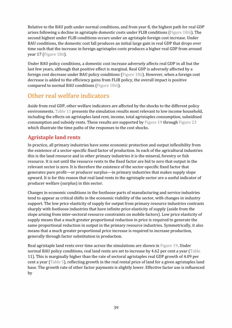
39
Relative to the BAU path under normal conditions, and from year 8, the highest path for real GDP
arises following a decline in agristaple domestic costs under FLIB conditions (Figure 18iii). The
second highest under FLIB conditions occurs under an agristaple foreign cost increase. Under
BAU conditions, the domestic cost fall produces an initial large gain in real GDP that drops over
time such that the increase in foreign agristaples costs produces a higher real GDP from around
year 17 (Figure 18ii).
Under BAU policy conditions, a domestic cost increase adversely affects real GDP in all but the
last few years, although that positive effect is marginal. Real GDP is adversely affected by a
foreign cost decrease under BAU policy conditions (Figure 18ii). However, when a foreign cost
decrease is added to the efficiency gains from FLIB policy, the overall impact is positive
compared to normal BAU conditions (Figure 18iii).
Other real welfare indicators
Aside from real GDP, other welfare indicators are affected by the shocks to the different policy
environments. Table 11 presents the simulation results most relevant to low income household,
including the effects on agristaples land rent, income, total agristaples consumption, subsidised
consumption and subsidy rents. These results are supported by Figure 19 through Figure 23
which illustrate the time paths of the responses to the cost shocks.
Agristaple land rents
In practice, all primary industries have some economic protection and output inflexibility from
the existence of a sector-specific fixed factor of production. In each of the agricultural industries
this is the land resource and in other primary industries it is the mineral, forestry or fish
resource. It is not until the resource rents to the fixed factor are bid to zero that output in the
relevant sector is zero. It is therefore the existence of the sector-specific fixed factor that
generates pure profit—or producer surplus—in primary industries that makes supply slope
upward. It is for this reason that real land rents in the agristaple sector are a useful indicator of
producer welfare (surplus) in this sector.
Changes in economic conditions in the footloose parts of manufacturing and service industries
tend to appear as critical shifts in the economic viability of the sector, with changes in industry
support. The low price elasticity of supply for output from primary resource industries contrasts
sharply with footloose industries that have infinite price elasticity of supply (aside from the
slope arising from inter-sectoral resource constraints on mobile factors). Low price elasticity of
supply means that a much greater proportional reduction in price is required to generate the
same proportional reduction in output in the primary resource industries. Symmetrically, it also
means that a much greater proportional price increase is required to increase production,
generally through factor substitution in production.
Real agristaple land rents over time across the simulations are shown in Figure 19. Under
normal BAU policy conditions, real land rents are set to increase by 4.62 per cent a year (Table
11). This is marginally higher than the rate of sectoral agristaples real GDP growth of 4.09 per
cent a year (Table 5), reflecting growth in the real rental price of land for a given agristaples land
base. The growth rate of other factor payments is slightly lower. Effective factor use is influenced
by

40
1) the neutral technical change assumption across factor inputs used to calibrate the model to a sector specific, constant, annual output growth rate, and
2) a land-specific technical change assumption that augments supply by the sector-specific output growth.
Across simulations, results for land rents are very similar to those for sectoral real GDP. Under
normal BAU conditions, land accounts for around 40 per cent of factor returns in year 1 and
around 50 per cent in year 20. Land rents also increase by 135.71 per cent over the 20 years
(Table 11). However, under FLIB and TLIB policy conditions, in year 20 land rents are 26.37 per
cent and 21.12 per cent lower than under BAU conditions, increasing more slowly from the base
year by 73.54 per cent and 85.93 per cent, respectively, relative to the base year (Table 11).
Other things being equal, reductions in land rents occur under domestic cost increases across all
three of the policy settings (Table 11 and Figure 8), between 78.45 per cent and 79.61 per cent.
Under BAU conditions, the significant fall in land rents in year 20 leaves rents at 49.2 per cent
below the base year value ending at US$4.87 billion (Table 11).
By design, foreign cost decreases that operate on the domestic economy as a world price
decrease, have small negative effects on land rents under BAU policy conditions in year 20.
Under FLIB conditions, they have large negative proportionate impacts (a fall of almost 50 per
cent), while the effects under TLIB conditions are in between. The efficient price signal involves
a marked decline in land rents and contraction in output. Under FLIB policy, the decline in real
agristaple land rents when there is a decline in foreign agristaple costs is 10.72 per cent in year
20 on account of the shock. While rents are higher in the base year, overall rents are 48.55 per
cent lower than otherwise in year 20 on account of the permanent decline in foreign agristaple
costs.
While the downside risk for land rents from a foreign cost decrease is higher under FLIB
conditions, the upside risk is also noteworthy. If foreign costs increase by 50 per cent, then the
FLIB policy environment gives the largest land rental gain relative to the base year at 105.36 per
cent. TLIB lies between the two policy extremes.
The largest overall increase in real land rents occurs under BAU policy conditions under a
domestic cost fall of 50 per cent. Real agristaples land rents increase by 870.13 per cent on the
base year or by 311.58 per cent on the value in year 20 without the permanent shock.

41
Figure 19 Agristaple land rents
i. BAU, FLIB and TLIB, normal policy conditions ii. BAU–Percentage deviation from normal BAU conditions
iii. FLIB–Percentage deviation from normal BAU conditions iv. TLIB–Percentage deviation from normal BAU conditions
%
5
10
15
20
25
1 4 7 10 13 16 19
BAU
TLIB
FLIB
Year
Billion 2004–05 US$ -100
%
100
200
300
400
1 4 7 10 13 16 19
dcost+
dcost-
fcost+
fcost-
Year
-100
%
100
200
300
400
1 4 7 10 13 16 19
dcost+
dcost-
fcost+
fcost-
Year
-100
%
100
200
300
400
1 4 7 10 13 16 19
dcost+
dcost-
fcost+
fcost-
Year
42
Low income households
The real income of low income households is a useful indicator of the purchasing power of this
group. In the ABARES/NCAP model it is measured as real GDP and is equivalent to factor income
payments plus any consumer subsidy rent. The factor income payments are principally wages
paid to unskilled labour.
A comparison of Figure 20 and Figure 22 for aggregate real GDP and real income for low income
households shows that the two series are generally moving together under normal BAU policy
conditions. Given the assumed mobility of unskilled labour throughout the economy (including
implicitly from rural to urban locations), and the relatively general growth pressures in the
economy, the increase in the real wage to unskilled labour results in real income growth of
5.19 per cent a year for low income households. It is apparent from this result that low income
households benefit closely from the economic growth in the general economy of 5.4 per cent a
year under normal BAU conditions.
There is one key difference between the impacts on aggregate GDP and real income for low
income households following agristaple cost shocks under BAU policy. This is the negative long
run effect of an agristaples domestic cost drop on low incomes (Figure 22ii). This result suggests
that the unskilled labour intensity of agristaples is higher than other sectors and that the real
wage needs to drop to ensure full employment in the long run. Interestingly, the domestic cost
drop has a significantly positive impact on low incomes in the medium run (years 6 to 15).
Under normal policy conditions, low income households experience higher real income in the
long run under FLIB and TLIB policy environments because of the efficiency implications of
agristaples tariff reform compared with the BAU policy environment (Figure 22i). However, in
the case of an increase in domestic or foreign costs, FLIB policy delivers an overall lower long-
run outcome for real income to low income households than under BAU. Overall, this suggests
that returns to unskilled labour are higher with a larger manufacturing sector in these instances.
Conversely, low income households receive higher long-run real income under FLIB and TLIB
policies than BAU policy under a domestic or foreign cost reduction (Table 11). This suggests
returns to unskilled labour are larger with a smaller manufacturing sector and a
correspondingly larger services sector.
Low income agristaples consumption and subsidy rents
As previously noted, under the BAU and TLIB policy environments in the model a targeted
consumer subsidy on agristaples is given to low income households from year 2 and this is quota
rationed. The ration quota is 50 per cent of base year consumption increasing over time by
1.3 per cent a year (the population growth rate). This level is assumed to be the minimum level
needed to support basic health needs for life. The low income consumer price—the subsidized
price—is held constant over time at half the market price in the base year. The discussion that
follows presents the simulation results in the context of Figure 21, which depicts the theoretical
welfare outcomes from varying consumption levels under a quota ration. These results are
summarised in Table 12.
Where the ration is less than the amount a consumer initially desires (as represented by the
ordinary demand curve), the ration does not have any direct efficiency effects and the level of
consumption is unchanged (see Table 12 case i and Figure 21).

43
Figure 20 Real income, low income households
i. BAU, FLIB and TLIB, normal policy conditions ii. BAU–Percentage deviation from normal BAU conditions
ii. FLIB–Percentage deviation from normal BAU conditions iv. TLIB–Percentage deviation from normal BAU conditions
50
100
150
200
250
1 4 7 10 13 16 19
BAU
TLIB
FLIB
Year
Billion 2004–05
US$
-10
-5
%
5
10
1 4 7 10 13 16 19
dcost+
dcost-
fcost+
fcost-
Year
-10
-5
%
5
10
1 4 7 10 13 16 19
dcost+
dcost-
fcost+
fcost-
Year
-10
-5
%
5
10
1 4 7 10 13 16 19
dcost+
dcost-
fcost+
fcost-
Year

44
Table 12 Consumer subsidy with quota ration outcomesa
Initial consumption is at QA (in absence of the regime). Final consumption is at QA, QB or QC where QA<QC<QB.
Final consumption
Consumer cost
Consumer rent
Government cost
Efficiency loss
Case depending on Quota location: (i) QA> Quota
QA PSUB*Quota+ (PMKT-PSUB)* (PMKT-PSUB)* Nil
PMKT* Quota Quota
(QA-Quota)
(ii) QB<Quota
QB PSUB*QB Nil (PMKT-PSUB)* AXB
QB
(iii) QC=Quota
QC PSUB*QC Nil (PMKT-PSUB)* AYC
QC a See Figure 21
Figure 21 Consumer subsidy with quota ration
Note: Quota is positioned for case (i). See Table 12.
Price
Demand
0 Quantity
(Market price)
(Subsidised price)
A
Quota
rent
B
C
X
Y

45
In this case, the economic impact of the subsidy on low income households occurs through the
real cash transfer from the government that the ration represents. This is the consumer subsidy
rent, which is equal to the net price subsidy times the quota ration. It is also the government
budget cost. Over-ration consumption is charged the market price. Since decisions are made at
the margin, the consumption outcome is unaffected directly by the subsidy.
Under normal BAU policy conditions, the low income support represents US$1.5 billion in year 2
and US$2.1 billion in year 20. This represents 2 per cent of low income household group income,
which declines to 1 per cent by year 20. In principle, this quota rationed subsidy would work
effectively as an income support. It would only be distorting in the extreme circumstance of a
shock that would cause consumption to fall below the quota in the absence of the income
support. However, with the support the shock consumption would move to the quota level
needed to support life. In the case that quota rents do not arise, the subsidy is only sufficient to
support life if the quota level is reached.
In the case that quota rents do arise, this is no different to a direct real cash transfer as a form of
social welfare. As modelled in this report, there is no direct government intervention involved in
buying or selling products for low income consumers. In an annual model, buying and selling to
meet the needs of low income consumers tends to coincide, negating the requirement of
modelling this behaviour
Consumption of agristaples by low income households exceeds the minimum quota ration
across all four simulation shocks. As a consequence, the consumer subsidy in the BAU and TLIB
simulations has no direct distorting effect on agristaples markets. Also under BAU and TLIB
policy conditions, there are real price ceilings that mitigate upward cost pressures. However,
price ceilings are distorting partly because they reduce the output response of producers and
the incomes of unskilled labour that produce agristaples and other goods. Raising the real
incomes of low income households through structural adjustment that draws unskilled labour to
the areas with the highest paying real wage is an inclusive growth strategy.
Under normal BAU policy conditions, agristaples consumption increases by 2.41 per cent
annually, reflecting low but assumed positive income elasticity (Table 11). Under normal FLIB
and TLIB conditions, higher income yields a 5.53 per cent and 4.87 per cent rise in consumption,
respectively.
From the direction of impacts in year 20 under BAU policy conditions, given the ceiling is in
place and income support from the consumer subsidy are both in place, the long-run impact on
agristaples cost shocks occurs through the real income impact. Under a foreign or a domestic
cost rise under BAU conditions in year 20, real income rises so the consumption impact is
positive (Table 11). This is the reverse of the short to medium-run impact that occurs when
consumption falls until the structural adjustment is completed, and reflects the initial
dominance of the real price impact rationing consumption (Figure 22ii).
Under FLIB policy conditions, a domestic or foreign cost fall has a positive effect on low income
household consumption of agristaples. This response augments the impact of liberalised
agristaples supply chain trade conditions and the removal of agristaples policies (Figure 22iii).
On the other hand, under FLIB policy conditions, an increase in foreign or domestic agristaple
costs leads to reductions in consumption relative to normal BAU policy conditions. These
reductions are largest in the short to medium term (Figure 22ii). In the case of a domestic cost
increase, the rate at which consumption declines slows before turning. When foreign costs
increase, there is structural adjustment which reduces the negative effect on consumption until
it is negligible in the long run.

46
Under TLIB policy, the spread of results from the normal policy environment is narrower
relative to FLIB policy outcomes under the agristaple cost shocks (Figure 22iv).
Consumer subsidy rents vary over time with economic conditions. In general, relative to normal
BAU conditions, the greater the market price faced by low income consumers, the greater the
rental support. This effect is seen in the results reported in Figure 23. As was reported in Table
2, the real price increases most under a foreign cost increase (Table 11 and Figure 23ii). As a
result, the subsidy rent is also highest under this shock, increasing by 20.53 per cent and 23.60
per cent relative to normal BAU and TLIB policy conditions, respectively. The same pattern is
observed for a domestic cost increase but at a lesser magnitude.
Under normal TLIB policy conditions, the real price of agristaples on the domestic market is
constant until year 11, after which it peaks in year 15 before declining to a higher overall level
relative to normal BAU conditions. Movements in the real rents of low income consumers are
similar to BAU policy conditions under upward cost pressure from domestic or foreign sources
(Figure 23ii and iii). The floor price binds when there is either a foreign or domestic cost
decrease in a TLIB environment, or when there is a domestic cost fall in a BAU policy
environment.

47
Figure 22 Agristaples consumption, low income households
i. BAU, FLIB and TLIB, normal conditions ii. BAU–Percentage deviation from BAU normal conditions
iii. FLIB–Percentage deviation from BAU normal conditions iv. TLIB–Percentage deviation from BAU normal conditions
%
2
4
6
8
10
1 4 7 10 13 16 19
BAU-total
FLIB
TLIB-total
Rationed part-BAU & TLIB
Year
Billion 2004–05 US$ -8
-6
-4
-2
%
2
4
1 4 7 10 13 16 19
dcost+
dcost-
fcost+
fcost-
Year
-15
-10
-5
%
5
10
15
20
1 4 7 10 13 16 19
dcost+
dcost-
fcost+
fcost-
Year
-15
-10
-5
%
5
10
15
20
1 4 7 10 13 16 19
dcost+
dcost-
fcost+
fcost-
Year
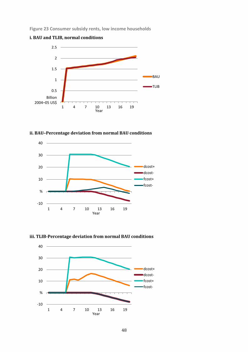
48
Figure 23 Consumer subsidy rents, low income households
i. BAU and TLIB, normal conditions
ii. BAU–Percentage deviation from normal BAU conditions
iii. TLIB-Percentage deviation from normal BAU conditions
%
0.5
1
1.5
2
2.5
1 4 7 10 13 16 19
BAU
TLIB
Year
Billion 2004–05 US$
-10
%
10
20
30
40
1 4 7 10 13 16 19
dcost+
dcost-
fcost+
fcost-
Year
-10
%
10
20
30
40
1 4 7 10 13 16 19
dcost+
dcost-
fcost+
fcost-
Year
49
5 Conclusion The objective of this project is to develop a model that can be used to assess the welfare effects
of Indian agristaples policies under different scenarios. To that end, the ABARES/NCAP
agristaples CGE model was developed. Using the model, analysis of three possible Indian
agristaples policy environments was carried out to estimate welfare changes—as measured by
GDP—as well as changes to key economic indicators across sectors and households. The analysis
provides an opportunity to demonstrate the effectiveness of the model at producing results that
are not only consistent with economic theory but also with existing Indian agristaples policies.
Where aggregate welfare is concerned, the simulation results demonstrate clearly that, for an
economy as a whole, fully liberalised agristaples markets (FLIB) lead to higher aggregate welfare
compared with policy environments that have experienced only tariff reform of the agristaples
and food processing sectors or no reform at all. This result is consistent across each scenario,
regardless of the type of agristaples cost shock. Conversely, aggregate welfare is lowest when no
policy reform has taken place (BAU) because of the distortions created by the simulated use of a
domestic price band policy and tariff policy.
For low income households, a fully liberalised policy environment (FLIB) also leads to higher
incomes and higher agristaples consumption over the long term compared with the other two
policy environments considered (BAU and TLIB). This result arises under normal policy
conditions and when there is either a foreign or domestic agristaples cost decrease (which
lowers the domestic price of agristaples). When there is a permanent increase in the foreign
agristaples costs (and hence in the market price of agristaples), there is less consumption in the
medium term by low income households. In the longer term, however, structural adjustment in
the form of higher agristaples production leads to higher income than in the other two policy
environments considered. Only when domestic agristaple costs increase is there a reduction in
consumption and income compared with the other two policy environment. This occurs because
of the absence of domestic support (consumption subsidies).
Removal of the tariffs which support the agristaples and food processing sector increases
aggregate welfare by stopping the under-consumption and over-production of domestic
agristaples when cheaper imports are available. Low income households benefit through an
increase in real incomes which is sufficient to offset any potentially deleterious effect on
minimum agristaples consumption following an increase in domestic or foreign agristaples
costs.
Agristaple price ceilings and floors are implemented to avoid undesirable effects on consumers
and producers of agristaples price hikes and cuts. However, they have costly unintended, market
distorting consequences. The simulation results demonstrate how government open market
interventions through an agristaples stockpile are unsustainable and require active trade
measures to maintain the price band. However, these trade measures are also distorting. For
example, following a domestic cost increase, imposing a fixed agristaples price ceiling causes
production to be substantially lower than it otherwise would be. The ceiling is supported using a
variable export tax or import subsidy, depending on economic conditions. In the face of a
domestic cost increase, a government agristaples stockpile can run out as product is moved from
the stockpile onto the open market in an attempt to constrain the price to no more than the price
ceiling. Once this occurs, variable trade measures are required to support the price ceiling. If
foreign costs increase, then the existence of a price ceiling can prevent domestic producers from
increasing production to fill the gap. In contrast to government stockpiling, private stockpiling

50
harnesses rather than suppresses economic price signals and, in so doing, could increase
aggregate economic wellbeing.
The illustrative results of this report are consistent with the different vested interests from the
consumption and production sides of the Indian agristaples market. An increase in foreign
agristaples costs affects world prices through their impact on world prices, and hence domestic
prices. As a result, the economic welfare of domestic producers increases (through higher land
rents) and that of consumers falls (through the loss in consumer surplus) in the market
considered. Conversely, a decrease in foreign agristaples costs lowers the economic welfare of
producers and increases the economic welfare of consumers. Addressing these gains and losses
with a market-distorting measure is sub-optimal for aggregate welfare when a first-best
measure is available, such as a direct income transfer to support a minimum quality of life.
The benefit of unsupported markets is that prices send a signal about how, where and when
scarce resources may be used to maximize aggregate economic welfare. As demonstrated in the
simulation analysis, direct income support or consumer subsidies may be used to protect the
incomes of low income households from agristaples shocks. Direct income support is not price
distorting because it assumes the development of a well-functioning taxation system and
associated social welfare system. Consumer subsidies for agristaples which target low income
households are also not price distorting provided the quota ration is less than the actual
consumption level.
The simulation analysis undertaken for this report has demonstrated the usefulness of the
economic framework underlying the ABARES/NCAP agristaples CGE model. The dynamics of the
results and the long-term results themselves are consistent with economic theory and with
expectations given existing Indian agristaples policies. The model’s framework has also been
shown to be effective at analysing market failures and potential market measures to address
them. Given these strengths, the ABARES/NCAP agristaples CGE model’s use for analysing a
range of alternative scenarios is implicit.
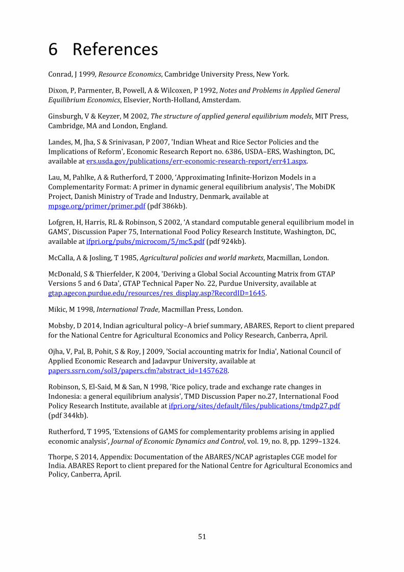
51
6 References Conrad, J 1999, Resource Economics, Cambridge University Press, New York.
Dixon, P, Parmenter, B, Powell, A & Wilcoxen, P 1992, Notes and Problems in Applied General
Equilibrium Economics, Elsevier, North-Holland, Amsterdam.
Ginsburgh, V & Keyzer, M 2002, The structure of applied general equilibrium models, MIT Press,
Cambridge, MA and London, England.
Landes, M, Jha, S & Srinivasan, P 2007, 'Indian Wheat and Rice Sector Policies and the
Implications of Reform', Economic Research Report no. 6386, USDA–ERS, Washington, DC,
available at ers.usda.gov/publications/err-economic-research-report/err41.aspx.
Lau, M, Pahlke, A & Rutherford, T 2000, ‘Approximating Infinite-Horizon Models in a
Complementarity Format: A primer in dynamic general equilibrium analysis', The MobiDK
Project, Danish Ministry of Trade and Industry, Denmark, available at
mpsge.org/primer/primer.pdf (pdf 386kb).
Lofgren, H, Harris, RL & Robinson, S 2002, ‘A standard computable general equilibrium model in
GAMS’, Discussion Paper 75, International Food Policy Research Institute, Washington, DC,
available at ifpri.org/pubs/microcom/5/mc5.pdf (pdf 924kb).
McCalla, A & Josling, T 1985, Agricultural policies and world markets, Macmillan, London.
McDonald, S & Thierfelder, K 2004, 'Deriving a Global Social Accounting Matrix from GTAP
Versions 5 and 6 Data', GTAP Technical Paper No. 22, Purdue University, available at
gtap.agecon.purdue.edu/resources/res_display.asp?RecordID=1645.
Mikic, M 1998, International Trade, Macmillan Press, London.
Mobsby, D 2014, Indian agricultural policy–A brief summary, ABARES, Report to client prepared
for the National Centre for Agricultural Economics and Policy Research, Canberra, April.
Ojha, V, Pal, B, Pohit, S & Roy, J 2009, 'Social accounting matrix for India', National Council of
Applied Economic Research and Jadavpur University, available at
papers.ssrn.com/sol3/papers.cfm?abstract_id=1457628.
Robinson, S, El-Said, M & San, N 1998, 'Rice policy, trade and exchange rate changes in
Indonesia: a general equilibrium analysis', TMD Discussion Paper no.27, International Food
Policy Research Institute, available at ifpri.org/sites/default/files/publications/tmdp27.pdf
(pdf 344kb).
Rutherford, T 1995, ‘Extensions of GAMS for complementarity problems arising in applied
economic analysis’, Journal of Economic Dynamics and Control, vol. 19, no. 8, pp. 1299–1324.
Thorpe, S 2014, Appendix: Documentation of the ABARES/NCAP agristaples CGE model for India. ABARES Report to client prepared for the National Centre for Agricultural Economics and Policy, Canberra, April.

52
Table 1 Agristaple markets under normal policy and market shocks in year 20
Policy environment Shock
Real price
Produc-tion
Consump-tion Exports Imports
Export tax/
Import subsidy
Export subsidy/
Import tariff
(index) ($US 2004-05 billion) (%) (%)
Wheat FLIB normal 1.19 30.41 30.45 0.00 0.04 na na
dcost+ 1.24 9.40 28.32 0.00 18.92 na na
dcost- 0.94 81.06 32.71 48.36 0.00 na na
fcost+ 1.49 35.96 29.66 6.31 0.00 na na
fcost- 1.00 24.81 30.51 0.00 5.70 na na
BAU normal 1.13 31.10 30.46 0.65 0.00 0.00 16.20
dcost+ 1.13 8.64 28.12 0.00 19.48 0.00 0.00
dcost- 1.13 89.19 32.94 56.25 0.00 0.00 36.50
fcost+ 1.33 34.55 29.86 4.68 0.00 2.90 0.00
fcost- 1.13 31.18 31.06 0.12 0.00 0.00 43.70
TLIB normal 1.18 30.39 30.39 0.00 0.00 0.00 0.00
dcost+ 1.24 9.53 28.27 0.00 18.75 0.00 0.00
dcost- 1.13 87.40 32.42 54.98 0.00 0.00 23.60
fcost+ 1.33 33.37 30.15 3.22 0.00 12.40 0.00
fcost- 1.13 29.11 30.44 0.00 1.33 0.00 14.70
Rice FLIB normal 1.06 15.12 11.63 3.49 0.00 na na
dcost+ 1.20 7.61 11.35 0.00 3.74 na na
dcost- 0.94 41.67 11.94 29.73 0.00 na na
fcost+ 1.45 18.75 11.02 7.74 0.00 na na
fcost- 0.87 12.49 11.69 0.80 0.00 na na
BAU normal 1.33 18.48 18.48 0.00 0.00 0.00 0.00
dcost+ 1.33 9.05 15.78 0.00 6.73 22.80 0.00
dcost- 1.13 46.43 23.04 23.39 0.00 0.00 29.40
fcost+ 1.33 18.19 15.36 2.83 0.00 2.70 0.00
fcost- 1.29 18.22 22.22 0.00 4.00 0.00 0.00
TLIB normal 1.13 16.04 11.53 4.52 0.00 0.00 7.60
dcost+ 1.20 7.68 11.33 0.00 3.65 0.00 0.00
dcost- 1.13 45.44 11.73 33.70 0.00 0.00 24.20
fcost+ 1.33 17.81 11.25 6.56 0.00 10.00 0.00
fcost- 1.13 16.05 11.53 4.53 0.00 0.00 32.80

53
Table 2 Agristaple markets, impacts of cost shocks
Policy environment
Shock Real price
Produc-tion
Consump-tion
Exports Imports Export tax/
import subsidy
Export subsidy/
Import tariff
(%) a (%) a (%) a (diff) a (diff) a (diff) a (diff) a
Wheat FLIB normal 0.00 0.00 0.00 0.00 0.00 na na
dcost+ 4.29 -69.08 -6.98 0.00 18.88 na na
dcost- -20.76 166.57 7.42 48.36 -0.04 na na
fcost+ 25.13 18.26 -2.59 6.31 -0.04 na na
fcost- -15.63 -18.41 0.22 0.00 5.67 na na
BAU normal 0.00 0.00 0.00 0.00 0.00 0.00 0.00
dcost+ 0.18 -72.23 -7.67 -0.65 19.48 0.00 -16.20
dcost- 0.00 186.73 8.14 55.60 0.00 0.00 20.30
fcost+ 17.42 11.06 -1.96 4.04 0.00 2.90 -16.20
fcost- 0.00 0.24 1.96 -0.52 0.00 0.00 27.50
TLIB normal 0.00 0.00 0.00 0.00 0.00 0.00 0.00
dcost+ 4.99 -68.65 -6.97 0.00 18.75 0.00 0.00
dcost- -4.31 187.61 6.68 54.98 0.00 0.00 23.60
fcost+ 12.35 9.81 -0.77 3.22 0.00 12.40 0.00
fcost- -4.31 -4.21 0.16 0.00 1.33 0.00 14.70
Rice FLIB normal 0.00 0.00 0.00 0.00 0.00 na na
dcost+ 13.62 -49.66 -2.40 -3.49 3.74 na na
dcost- -11.26 175.62 2.66 26.24 0.00 na na
fcost+ 37.56 24.04 -5.26 4.25 0.00 na na
fcost- -17.50 -17.40 0.52 -2.69 0.00 na na
BAU normal 0.00 0.00 0.00 0.00 0.00 0.00 0.00
dcost+ 0.00 -51.01 -14.58 0.00 6.73 22.80 0.00
dcost- -14.83 151.27 24.67 23.39 0.00 0.00 29.40
fcost+ 0.00 -1.59 -16.89 2.83 0.00 2.70 0.00
fcost- -2.94 -1.41 20.25 0.00 4.00 0.00 0.00
TLIB normal 0.00 0.00 0.00 0.00 0.00 0.00 0.00
dcost+ 6.19 -52.15 -1.72 -4.52 3.65 0.00 -7.60
dcost- 0.00 183.21 1.77 29.19 0.00 0.00 16.60
fcost+ 17.42 11.00 -2.44 2.05 0.00 10.00 -7.60
fcost- 0.00 0.06 0.00 0.01 0.00 0.00 25.20
a Expressed relative to normal conditions of the same policy environment (FLIB, BAU, TLIB).

54
Table 3 Agristaple markets, comparison of normal policy environments in year 20
Policy environment
Real price
Produc-tion
Consump-tion
Exports Imports Export tax/
Import subsidy
Export subsidy/
Import tariff
(% chg)a (% chg)a (% chg)a (diff)a (diff)a (diff) a (diff)a Wheat
BAU
0.00 0.00 0.00 0.00 0.00 0.00 0.00 FLIB
5.22 -2.23 -0.04 -0.65 0.04 na na
TLIB
4.51 -2.30 -0.23 -0.65 0.00 0.00 -0.16 Rice
BAU
0 0 0 0.00 0.00 0.00 0.00 FLIB
-20.41 -18.18 -37.07 3.49 0.00 na na
TLIB -14.83 -13.18 -37.61 4.52 0.00 0.00 0.08 a Relative to BAU.

55
Table 4 Sectoral output ($US 2004–05 billion)
Policy Environment Shock Agristaples
Other agriculture
Other primary Manuf. Services
year 1- BAU 30.71 127.72 37.67 465.09 537.33
year 20 BAU normal 49.58 274.23 96.11 1020.73 1721.02
dcost+ 17.69 273.01 96.33 1281.72 1721.80
dcost- 135.62 275.94 94.94 644.94 1696.46
fcost+ 52.73 266.71 97.22 1337.74 1763.09
fcost- 49.40 275.40 95.70 912.01 1697.20
FLIB normal 45.53 282.52 95.76 890.85 1759.11
dcost+ 17.01 283.92 95.68 940.28 1747.45
dcost- 122.73 278.29 96.19 898.41 1786.96
fcost+ 54.72 278.58 96.01 925.21 1771.79
fcost- 37.30 284.49 95.65 887.31 1752.40
TLIB normal 46.43 283.85 95.60 823.88 1756.04
dcost+ 17.20 285.33 95.51 882.33 1743.36
dcost- 132.84 283.10 95.39 594.29 1772.88
fcost+ 51.18 280.68 95.87 890.47 1765.86
fcost- 45.16 284.48 95.55 810.17 1754.06
year 20 Comparison of sectoral growth under normal conditions
avg ann growth
avg ann growth
avg ann growth
avg ann growth
avg ann growth
BAU
2.55 4.10 5.05 4.22 6.32
(%)a (%)a (%)a (%)a (%)a
BAU
0.00 0.00 0.00 0.00 0.00
FLIB
-8.18 3.02 -0.37 -12.72 2.21
TLIB
-6.35 3.51 -0.53 -19.29 2.03
year 20 Comparison of shocked relative to normal environment
(%)b (%)b (%)b (%)b (%)b
BAU normal 0.00 0.00 0.00 0.00 0.00
dcost+ -64.32 -0.45 0.22 25.57 0.04
dcost- 173.52 0.62 -1.22 -36.82 -1.43
fcost+ 6.35 -2.74 1.15 31.06 2.44
fcost- -0.37 0.43 -0.43 -10.65 -1.38
FLIB normal 0.00 0.00 0.00 0.00 0.00
dcost+ -62.63 0.49 -0.09 5.55 -0.66
dcost- 169.57 -1.50 0.45 0.85 1.58
fcost+ 20.18 -1.40 0.26 3.86 0.72
fcost- -18.07 0.70 -0.11 -0.40 -0.38
TLIB normal 0.00 0.00 0.00 0.00 0.00
dcost+ -62.95 0.52 -0.10 7.10 -0.72
dcost- 186.09 -0.27 -0.22 -27.87 0.96
fcost+ 10.22 -1.12 0.28 8.08 0.56
fcost- -2.74 0.22 -0.06 -1.66 -0.11
a Percentage change from normal BAU. b Percentage change from the same normal policy environment.

56
Table 5 Sectoral real GDPa ($US 2004–05 billion)
Policy environ-ment Shock Agristaples
Other ag
Other primary Manuf. Services Totalb
year 1- BAU 21.78 90.50 29.79 118.08 306.93 567.08
year 20 BAU normal 46.66 194.97 75.03 239.92 987.49 1544.06
dcost+ 15.30 194.05 75.17 281.78 984.77 1551.07
dcost- 141.31 197.58 74.50 181.44 982.08 1576.89
fcost+ 55.72 187.74 75.28 287.16 1001.81 1607.71
fcost- 45.62 196.10 74.79 233.42 976.00 1525.92
FLIB normal 37.79 223.63 82.56 200.50 1119.15 1663.63
dcost+ 13.12 223.59 82.19 210.99 1106.73 1636.63
dcost- 101.10 223.40 83.70 203.67 1148.13 1759.99
fcost+ 64.55 215.67 81.36 204.44 1108.28 1674.29
fcost- 23.79 227.99 83.26 201.73 1125.24 1662.01
TLIB normal 39.74 224.46 82.38 185.43 1117.23 1649.24
dcost+ 13.26 224.77 82.07 198.14 1104.87 1623.09
dcost- 136.39 224.42 82.33 133.93 1132.60 1709.67
fcost+ 52.58 219.51 81.90 198.49 1113.59 1666.07
fcost- 37.29 225.49 82.50 182.74 1118.22 1646.23
year 20 Comparison of normal policy environments to BAU
avg ann growth
(%)
avg ann growth
(%)
avg ann growth
(%)
avg ann growth
(%)
avg ann growth
(%)
avg ann growth
(%)
BAU
4.09 4.12 4.98 3.80 6.34 5.41
(%)c (%)c (%)c (%)c (%)c (%)c
BAU
0.00 0.00 0.00 0.00 0.00 0.00
FLIB
-19.01 14.70 10.04 -16.43 13.33 7.74
TLIB
-14.84 15.12 9.81 -22.71 13.14 6.81
year 20 Comparison of shocked relative to normal environment
(% chg) (% chg) (% chg) (% chg) (% chg) (% chg)
BAU normal 0.00 0.00 0.00 0.00 0.00 0.00
dcost+ -67.22 -0.47 0.20 17.45 -0.28 0.45
dcost- 202.84 1.34 -0.70 -24.38 -0.55 2.13
fcost+ 19.41 -3.71 0.33 19.69 1.45 4.12
fcost- -2.24 0.58 -0.31 -2.71 -1.16 -1.17
FLIB normal 0.00 0.00 0.00 0.00 0.00 0.00
dcost+ -65.27 -0.02 -0.45 5.23 -1.11 -1.62
dcost- 167.52 -0.10 1.38 1.58 2.59 5.79
fcost+ 70.82 -3.56 -1.45 1.97 -0.97 0.64
fcost- -37.06 1.95 0.85 0.62 0.54 -0.10
TLIB normal 0.00 0.00 0.00 0.00 0.00 0.00
dcost+ -66.64 0.14 -0.39 6.85 -1.11 -1.59
dcost- 243.22 -0.02 -0.06 -27.77 1.38 3.66
fcost+ 32.31 -2.21 -0.58 7.05 -0.33 1.02
fcost- -6.17 0.46 0.14 -1.45 0.09 -0.18 a Real GDP as value added factor incomes deflated by the CPI b This is real GDP excluding the consumer subsidy rent. c Percentage change from normal BAU.

57
Table 6 Change in sectoral contribution to total GDP a
Policy Environment Shock Agristaples
Other agriculture
Other primary Manuf. Services Totalb
(%) (%) (%) (%) (%) (%)
Normal conditions
BAU
0 0 0 0 0 0
FLIB
-0.57 1.86 0.49 -2.55 8.53 7.74
TLIB
-0.45 1.91 0.48 -3.53 8.40 6.81
Shocked conditions BAU
dcost+ -2.03 -0.06 0.01 2.71 -0.18 0.45
dcost- 6.13 0.17 -0.03 -3.79 -0.35 2.13
fcost+ 0.59 -0.47 0.02 3.06 0.93 4.12
fcost- -0.07 0.07 -0.02 -0.42 -0.74 -1.17
FLIB
dcost+ -1.48 0.00 -0.02 0.63 -0.75 -1.62
dcost- 3.81 -0.01 0.07 0.19 1.74 5.79
fcost+ 1.61 -0.48 -0.07 0.24 -0.65 0.64
fcost- -0.84 0.26 0.04 0.07 0.37 -0.10
TLIB
dcost+ -1.61 0.02 -0.02 0.77 -0.75 -1.59
dcost- 5.86 0.00 0.00 -3.12 0.93 3.66
fcost+ 0.78 -0.30 -0.03 0.79 -0.22 1.02
fcost- -0.15 0.06 0.01 -0.16 0.06 -0.18
a Using sectoral value share in real GDP under normal conditions as weights. b This is real GDP excluding the subsidy rent.

58
Table 7 Unskilled labour use ($US 2004–05 billion)
Policy environment Shock Agristaples
Other agriculture
Other primary Manuf. Services Total
year 1- BAU 8.41 34.96 9.00 47.54 100.30 200.21
year 20
BAU normal 8.17 37.55 11.16 46.01 153.01 255.90
dcost+ 3.50 37.07 11.10 52.17 152.05 255.90
dcost- 16.61 38.31 11.17 37.26 152.55 255.90
fcost+ 8.75 34.82 10.78 51.44 150.12 255.90
fcost- 8.12 38.03 11.21 46.49 152.04 255.90
FLIB normal 6.90 40.45 11.59 34.02 162.93 255.90
dcost+ 3.18 41.08 11.71 36.31 163.61 255.90
dcost- 12.62 38.62 11.26 33.13 160.27 255.90
fcost+ 9.81 39.02 11.40 34.62 161.05 255.90
fcost- 4.99 41.18 11.69 34.22 163.82 255.90
TLIB normal 7.25 41.04 11.69 31.78 164.15 255.90
dcost+ 3.24 41.69 11.80 34.42 164.74 255.90
dcost- 15.92 40.74 11.60 22.81 164.83 255.90
fcost+ 8.64 39.80 11.51 33.71 162.24 255.90
fcost- 6.97 41.29 11.72 31.37 164.55 255.90
year 20
(diff) (diff) (diff) (diff) (diff) (diff)
BAU
-0.24 2.59 2.16 -1.54 52.71 55.69
(diff)a (diff)a (diff)a (diff)a (diff)a
BAU
0.00 0.00 0.00 0.00 0.00
FLIB
-1.27 2.91 0.43 -11.99 9.92
TLIB
-0.92 3.49 0.52 -14.23 11.14
(diff)b (diff)b (diff)b (diff)b (diff)b (diff)b
BAU normal 0.00 0.00 0.00 0.00 0.00 na
dcost+ -4.67 -0.48 -0.07 6.17 -0.96 na
dcost- 8.43 0.77 0.01 -8.75 -0.46 na
fcost+ 0.58 -2.73 -0.39 5.43 -2.89 na
fcost- -0.05 0.48 0.05 0.49 -0.97 na
FLIB normal 0.00 0.00 0.00 0.00 0.00 na
dcost+ -3.72 0.63 0.12 2.30 0.68 na
dcost- 5.72 -1.84 -0.33 -0.88 -2.67 na
fcost+ 2.91 -1.43 -0.20 0.60 -1.88 na
fcost- -1.91 0.73 0.10 0.20 0.88 na
TLIB normal 0.00 0.00 0.00 0.00 0.00 na
dcost+ -4.01 0.66 0.12 2.64 0.59 na
dcost- 8.66 -0.29 -0.08 -8.97 0.68 na
fcost+ 1.39 -1.24 -0.18 1.93 -1.91 na
fcost- -0.28 0.25 0.04 -0.41 0.40 na
a Change from normal BAU.
b Change from the same normal policy environment.
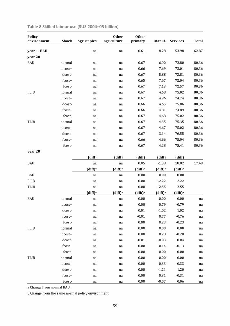
59
Table 8 Skilled labour use ($US 2004–05 billion)
Policy environment Shock Agristaples
Other agriculture
Other primary Manuf. Services Total
year 1- BAU na na 0.61 8.28 53.98 62.87
year 20
BAU normal na na 0.67 6.90 72.80 80.36
dcost+ na na 0.66 7.69 72.01 80.36
dcost- na na 0.67 5.88 73.81 80.36
fcost+ na na 0.65 7.67 72.04 80.36
fcost- na na 0.67 7.13 72.57 80.36
FLIB normal na na 0.67 4.68 75.02 80.36
dcost+ na na 0.67 4.96 74.74 80.36
dcost- na na 0.66 4.65 75.06 80.36
fcost+ na na 0.66 4.81 74.89 80.36
fcost- na na 0.67 4.68 75.02 80.36
TLIB normal na na 0.67 4.35 75.35 80.36
dcost+ na na 0.67 4.67 75.02 80.36
dcost- na na 0.67 3.14 76.55 80.36
fcost+ na na 0.66 4.66 75.04 80.36
fcost- na na 0.67 4.28 75.41 80.36
year 20
(diff) (diff) (diff) (diff) (diff)
BAU
na na 0.05 -1.38 18.82 17.49
(diff)a (diff)a (diff)a (diff)a (diff)a
BAU
na na 0.00 0.00 0.00
FLIB
na na 0.00 -2.22 2.22
TLIB
na na 0.00 -2.55 2.55
(diff)a (diff)a (diff)a (diff)a (diff)a
BAU normal na na 0.00 0.00 0.00 na
dcost+ na na 0.00 0.79 -0.79 na
dcost- na na 0.01 -1.02 1.02 na
fcost+ na na -0.01 0.77 -0.76 na
fcost- na na 0.00 0.23 -0.23 na
FLIB normal na na 0.00 0.00 0.00 na
dcost+ na na 0.00 0.28 -0.28 na
dcost- na na -0.01 -0.03 0.04 na
fcost+ na na 0.00 0.14 -0.13 na
fcost- na na 0.00 0.00 0.00 na
TLIB normal na na 0.00 0.00 0.00 na
dcost+ na na 0.00 0.33 -0.33 na
dcost- na na 0.00 -1.21 1.20 na
fcost+ na na 0.00 0.31 -0.31 na
fcost- na na 0.00 -0.07 0.06 na
a Change from normal BAU.
b Change from the same normal policy environment.

60
Table 9 General capital use ($US 2004–05 billion)
Policy environment Shock Agristaples
Other agriculture
Other primary Manuf. Services Total
year 1- BAU 6.39 26.54 21.81 77.49 190.35 322.58
year 20 BAU normal 12.11 55.63 52.80 151.69 573.15 845.37
dcost+ 5.27 55.76 53.27 183.94 574.41 872.64
dcost- 23.91 55.17 51.35 105.77 559.67 795.87
fcost+ 14.12 56.19 55.51 196.40 607.11 929.33
fcost- 11.84 55.44 52.15 141.92 561.91 823.26
FLIB normal 9.55 55.94 51.16 117.88 572.11 806.64
dcost+ 4.32 55.77 50.75 123.56 563.78 798.17
dcost- 18.49 56.57 52.63 121.63 594.80 844.11
fcost+ 14.03 55.79 52.01 124.05 583.96 829.84
fcost- 6.79 56.04 50.77 116.68 566.19 796.47
TLIB normal 9.87 55.81 50.73 108.30 567.90 792.60
dcost+ 4.33 55.67 50.32 115.19 559.22 784.73
dcost- 21.79 55.78 50.70 78.25 576.36 782.88
fcost+ 12.13 55.82 51.52 118.49 577.73 815.69
fcost- 9.42 55.80 50.57 106.24 565.94 787.96
Year 20 Comparison of normal policy environments to BAU
(diff) (diff) (diff) (diff) (diff) (diff)
BAU
5.72 29.09 30.99 74.19 382.80 522.79
(diff)a (diff)a (diff)a (diff)a (diff)a (diff)a
BAU
0.00 0.00 0.00 0.00 0.00 0.00
FLIB
-2.56 0.31 -1.63 -33.81 -1.04 -38.74
TLIB
-2.24 0.18 -2.07 -43.39 -5.25 -52.77
Year 20 Comparison of shocked relative to normal environment
(diff)b (diff)b (diff)b (diff)b (diff)b (diff)b
BAU normal 0.00 0.00 0.00 0.00 0.00 0.00
dcost+ -6.84 0.13 0.48 32.25 1.26 27.27
dcost- 11.80 -0.46 -1.44 -45.92 -13.48 -49.50
fcost+ 2.02 0.56 2.72 44.71 33.96 83.96
fcost- -0.27 -0.19 -0.64 -9.77 -11.24 -22.11
FLIB normal 0.00 0.00 0.00 0.00 0.00 0.00
dcost+ -5.23 -0.17 -0.41 5.68 -8.34 -8.46
dcost- 8.94 0.63 1.47 3.75 22.69 37.47
fcost+ 4.48 -0.15 0.84 6.17 11.84 23.20
fcost- -2.76 0.10 -0.39 -1.20 -5.92 -10.16
TLIB normal 0.00 0.00 0.00 0.00 0.00 0.00
dcost+ -5.53 -0.14 -0.41 6.89 -8.68 -7.88
dcost- 11.93 -0.03 -0.02 -30.05 8.45 -9.73
fcost+ 2.26 0.02 0.79 10.19 9.83 23.09
fcost- -0.45 -0.01 -0.16 -2.06 -1.96 -4.64
a Difference from normal BAU. b Difference from the same normal policy environment.
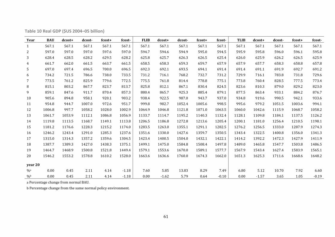
61
Table 10 Real GDP ($US 2004–05 billion)
Year BAU dcost+ dcost- fcost+ fcost- FLIB dcost+ dcost- fcost+ fcost- TLIB dcost+ dcost- fcost+ fcost-
1 567.1 567.1 567.1 567.1 567.1 567.1 567.1 567.1 567.1 567.1 567.1 567.1 567.1 567.1 567.1
2 597.0 597.0 597.0 597.6 597.0 594.7 594.6 594.9 595.0 594.5 595.9 595.8 596.0 596.1 595.8
3 628.4 628.5 628.2 629.5 628.2 625.8 625.7 626.3 626.5 625.4 626.0 625.9 626.2 626.5 625.9
4 661.7 662.0 661.5 663.7 661.5 658.5 658.3 659.3 659.7 657.9 657.9 657.7 658.3 658.8 657.8
5 697.0 697.4 696.5 700.0 696.5 692.3 692.1 693.5 694.1 691.4 691.4 691.1 691.9 692.7 691.2
6 734.2 721.5 786.6 738.0 733.5 731.2 716.1 768.2 732.7 731.2 729.9 716.1 783.8 731.8 729.6
7 773.5 761.2 825.9 779.6 772.5 775.5 761.8 814.4 778.8 775.1 773.8 760.4 828.5 777.5 773.4
8 815.1 803.2 867.7 823.7 813.7 825.8 812.1 867.1 830.4 824.5 823.6 810.3 879.0 829.2 823.0
9 859.1 847.6 911.7 870.4 857.3 880.4 865.7 925.3 885.4 879.1 877.5 863.4 933.1 884.2 876.7
10 905.6 894.8 958.1 920.1 903.2 938.4 922.5 987.0 943.7 937.0 934.8 919.6 990.5 942.1 933.6
11 954.8 944.7 1007.0 972.6 951.7 999.8 982.7 1052.4 1005.6 998.5 995.6 979.2 1051.5 1003.6 994.1
12 1006.8 997.7 1058.2 1028.0 1002.9 1064.9 1046.8 1121.8 1071.0 1063.5 1060.0 1042.6 1115.9 1068.7 1058.2
13 1061.7 1053.9 1112.1 1086.8 1056.9 1133.7 1114.7 1195.2 1140.3 1132.4 1128.1 1109.8 1184.1 1137.5 1126.2
14 1119.8 1113.5 1168.7 1149.1 1113.8 1206.5 1186.8 1272.8 1213.6 1205.4 1200.1 1181.0 1256.4 1210.5 1198.1
15 1181.2 1176.6 1228.3 1215.2 1174.0 1283.5 1263.0 1355.1 1291.1 1282.5 1276.2 1256.5 1333.0 1287.9 1274.3
16 1246.2 1243.4 1291.0 1285.3 1237.6 1351.6 1330.0 1427.6 1359.7 1350.5 1343.4 1322.5 1400.8 1356.0 1341.3
17 1315.0 1314.3 1357.2 1359.6 1304.5 1423.4 1400.5 1504.0 1432.1 1422.1 1414.2 1392.2 1472.3 1427.9 1411.9
18 1387.7 1389.3 1427.0 1438.3 1375.1 1499.1 1475.0 1584.8 1508.4 1497.8 1489.0 1465.8 1547.7 1503.8 1486.5
19 1464.7 1468.9 1500.8 1521.8 1449.4 1579.1 1553.6 1670.0 1589.1 1577.7 1567.9 1543.4 1627.4 1583.9 1565.1
20 1546.2 1553.2 1578.8 1610.2 1528.0 1663.6 1636.6 1760.0 1674.3 1662.0 1651.3 1625.3 1711.6 1668.6 1648.2 year 20
%a 0.00 0.45 2.11 4.14 -1.18 7.60 5.85 13.83 8.29 7.49 6.80 5.12 10.70 7.92 6.60
%b 0.00 0.45 2.11 4.14 -1.18 0.00 -1.62 5.79 0.64 -0.10 0.00 -1.57 3.65 1.05 -0.19
a Percentage change from normal BAU. b Percentage change from the same normal policy environment.

62
Table 11 Other real welfare indicators ($US 2004–05 billion)
Policy
Low income households environment
Agristaples
Shock Agristaples
land rent Income Total
consumption Subsidised
consumption Subsidy
rent
year 1- BAU 9.58 75.46 4.72 0.00 0.00
year 20 BAU normal 22.58 197.38 7.43 3.02 2.09
dcost+ 4.87 200.59 7.48 3.02 2.10
dcost- 92.95 193.12 7.43 3.02 1.93
fcost+ 28.39 214.39 7.55 3.02 2.52
fcost- 21.94 194.38 7.40 3.02 2.06
FLIB normal 16.63 199.61 7.84 0.00 0.00
dcost+ 3.56 194.81 7.64 0.00 0.00
dcost- 60.12 214.67 8.28 0.00 0.00
fcost+ 34.15 203.62 7.43 0.00 0.00
fcost- 8.55 197.92 8.01 0.00 0.00
TLIB normal 17.81 197.86 7.79 3.02 2.04
dcost+ 3.63 193.50 7.62 3.02 2.23
dcost- 87.84 199.70 7.88 3.02 1.93
fcost+ 26.00 203.47 7.66 3.02 2.52
fcost- 16.29 196.74 7.82 3.02 1.93
year 20
avg ann growth
(%)
avg ann growth
(%)
avg ann growth
(%)
avg ann growth
(%)
avg ann growth
(%)
BAU
4.62 5.19 2.41 na na
(%)a (%)a (%)a (%)a (%)a
BAU
0.00 0.00 0.00 0.00 0.00
FLIB
-26.37 1.13 5.53 -100.00 -100.00
TLIB
-21.12 0.24 4.87 0.00 -2.48
(%)b (%)b (%)b (%)b (%)b
BAU normal 0.00 0.00 0.00 0.00 0.00
dcost+ -78.45 1.63 0.70 0.00 0.14
dcost- 311.58 -2.16 0.03 0.00 -7.83
fcost+ 25.71 8.62 1.64 0.00 20.53
fcost- -2.86 -1.52 -0.47 0.00 -1.53
FLIB normal 0.00 0.00 0.00 na na
dcost+ -78.58 -2.40 -2.56 na na
dcost- 261.56 7.55 5.55 na na
fcost+ 105.36 2.01 -5.28 na na
fcost- -48.55 -0.84 2.14 na na
TLIB normal 0.00 0.00 0.00 0.00 0.00
dcost+ -79.61 -2.20 -2.27 0.00 9.11
dcost- 393.12 0.93 1.10 0.00 -5.48
fcost+ 45.94 2.84 -1.67 0.00 23.60
fcost- -8.57 -0.57 0.39 0.00 -5.48
a Percentage change from normal BAU. b Percentage change from the same normal policy environment.