Embed Size (px)
Citation preview

UNIVERSITY OF LIÈGE FACULTY OF APPLIED SCIENCES
AEROSPACE AND MECHANICAL ENGINEERING DEPARTMENT THERMODYNAMICS LABORATORY
STUDY, MODELLING AND ANALYSIS OF HEAT PUMPING SOLUTIONS IN A COMMERCIAL BUILDING
Stéphane Bertagnolio
Thesis Submitted in Partial Fulfilment of the Requirements for the Degree of Electromechanical Civil Engineer
(Energetic Engineering)
June 2007

ACKNOWLEDGEMENTS
I am grateful to Professor J.Lebrun who oversaw this work and
enabled me to follow this great project. I thank him for his trust
and supervision.
I also thank Jules Hannay and Cleide Aparecida Silva for their
suggestions and their help.
Special thank to Bernard Georges for his permanent availability
to reply to any question, and to Vincent Lemort for his advises.
I also thank Philippe Ngendakumana, Philippe André and
Georges Heyen for their corrections.
A great thank to Pierre Gustin, Sylvain Quoilin, Laurie Detroux
and Ludovic Buckinx for their support, their friendship and the
great environment of work.
Lastly, I want to thank all the people who were a real support for
me during the five last years.

ABSTRACT
This work is carried out in the frame of the IEA-ECBCS (International Energy Agency –
Energy Conservation in Buildings and Community Systems) Annex48: “Heat Pumping and
Reversible Air Conditioning”. The aim of this work is to study the possibility of integration of
a reversible heat pumping system into the existing HVAC system of a “commercial” building
(which includes laboratories).
A pre-audit of the actual HVAC installation is carried out and presented. Numerical models of
the building and of the coupled HVAC installation are developed and implemented on EES
(Engineering Equation Solver, ©F-Chart Software) to run yearly simulations. The main
retrofit opportunity is the use of reversible heat pumping, with the extracted air as heat source,
to heat the building. Other retrofit possibilities, as “change over” technique or cool thermal
energy storage, are also modelled, simulated and analysed. The environmental and
economical aspects of each retrofit opportunity are approached.
The reversible heat pumping coupled with a change over technique is generally able to satisfy
the heating demand of the building. However some interventions of the existing natural gas
condensing boilers, as back boosting devices, are sometimes necessary during winter. The
economical and environmental studies reveal a quite short payback time and a significant
reduction of CO2 emissions. The advantages of the cool thermal storage solution are not
obvious and have not been highlighted in the present case.

RÉSUMÉ
Ce travail est réalisé dans le cadre du projet IEA-ECBCS (International Energy Agency –
Energy Conservation in Buildings and Community Systems) Annex48 : « Heat Pumping and
Reversible Air Conditioning ». Le but de ce travail est l’étude de la possibilité d’intégration
d’un système de pompe à chaleur réversible dans l’actuelle installation de conditionnement
d’air d’un bâtiment commercial comprenant des laboratoires.
Un pre-audit de l’actuelle installation est réalisé et présenté. Plusieurs modèles numériques du
bâtiment et de l’installation HVAC sont développés et compilés au moyen du programme
EES (Engineering Equation Solver, ©F-Chart Software) en vue de réaliser une simulation
annuelle. La principale possibilité de modification de l’installation actuelle est l’utilisation
d’un système de pompe à chaleur réversible, utilisant l’air extrait comme source de chaleur,
pour répondre à la demande de chaud du bâtiment. D’autres opportunités, comme l’utilisation
d’une technique de « change over » ou d’un système de stockage de froid, sont aussi
modélisées, simulées et analysées. Les aspects environnementaux et économiques sont
également abordés.
L’utilisation d’un système de pompe à chaleur, couplé à une technique de « change over »,
est, en général, capable de satisfaire la demande de chaud du bâtiment. Toutefois,
l’intervention des chaudières au gaz naturel, comme dispositif de chauffage auxiliaire, est
parfois nécessaire pendant la période hivernale. Les études économiques et environnementales
donnent un temps de retour sur investissement relativement court et une réduction
significative des émissions de CO2. Les avantages du système de stockage de froid ne sont
pas évidents et n’ont pas pu être mis en avant dans le cas présent.
INTRODUCTION.................................................................................................................... 1
PART I : DESCRIPTION & PRE-AUDIT OF THE EXISTING SYSTEM...................... 2
I.1. BUILDING.......................................................................................................................... 3
I.1.1. Dividing the building in zones .................................................................................. 3
I.1.2. Orientations and exposure ........................................................................................ 4
I.1.3. Building thermal characteristics............................................................................... 5
I.2. AIR CONDITIONING SYSTEM ............................................................................................. 6
I.2.1. Offices Floor ............................................................................................................. 6
I.2.2. Laboratories Floor.................................................................................................... 8
I.2.3. Fourth & Fifth Zone.................................................................................................. 9
I.3. REFRIGERATION & HEATING PLANT ............................................................................... 10
I.3.1. Heat Production...................................................................................................... 10
I.3.2. Cold Production...................................................................................................... 10
I.4. WATER DISTRIBUTION NETWORK................................................................................... 11
I.5. PRE-AUDIT OF THE INSTALLATION .................................................................................. 13
I.5.1. Electricity & Gas Consumptions ............................................................................ 13
I.5.2. Thermal Signature .................................................................................................. 17
I.6. CONCLUSIONS ................................................................................................................. 19
I.7. RETROFIT OPPORTUNITIES .............................................................................................. 20
PART II : MODELLING OF THE INSTALLATION....................................................... 22
II.1. AIM & PHILOSOPHY OF THE MODELLING PHASE........................................................... 23
II.2. BUILDING MODEL.......................................................................................................... 24
II.2.1. Zone Sensible Heat Balance .................................................................................. 25
II.2.2. Structure Energy Balance...................................................................................... 25
II.2.3. Fabric Heat Transmission ..................................................................................... 26
II.2.4. Ventilation Enthalpy Flow rate ............................................................................. 27
II.2.5. Sensible Heat Gains............................................................................................... 27
II.2.6. Zone Water Balance .............................................................................................. 29
II.2.7. Building Model Parameters................................................................................... 30
II.3. HVAC SYSTEM MODEL ................................................................................................ 32
II.3.1. Air Handling Unit Model....................................................................................... 32
II.3.1.1. Heating Coil Model ........................................................................................ 33
II.3.1.2. Cooling Coil Model ........................................................................................ 36
II.3.1.3. Recovery Loop Model .................................................................................... 41
II.3.1.4. Steam Humidifier Model ................................................................................ 44
II.3.1.5. Fan Model....................................................................................................... 45
II.3.1.6. Duct Model ..................................................................................................... 45
II.3.1.7. Air Handling Unit Global Model Parameters................................................. 46
II.3.2. Terminal Unit Model ............................................................................................. 47
II.3.3. Cooling Plant Model ............................................................................................. 48
II.3.3.1. Air Cooled Chiller .......................................................................................... 48
II.3.3.2. Chilled Water Network................................................................................... 51
II.3.4. Heating Plant Model ............................................................................................. 51
II.3.4.1. Condensing Boiler .......................................................................................... 51
II.3.4.2. Hot Water Network ........................................................................................ 51
II.4. INPUTS OF THE MODEL ................................................................................................. 52
II.4.1. Weather Data......................................................................................................... 52
II.4.2. Occupancy Rates ................................................................................................... 53

II.4.2.1. Offices ............................................................................................................ 53
II.4.2.2. Laboratories .................................................................................................... 53
II.4.3. Control Laws ......................................................................................................... 54
II.4.3.1. Offices ............................................................................................................ 54
II.4.3.2. Laboratories .................................................................................................... 56
II.5. OUTPUTS OF THE MODEL.............................................................................................. 56
PART III : SIMULATION RESULTS AND ANALYSIS.................................................. 57
III.1. INTRODUCTION............................................................................................................. 58
III.2. PRESENT SITUATION – SIMULATION RESULTS.............................................................. 58
III.2.1. Temperature Profiles............................................................................................ 58
III.2.1.1. Laboratories................................................................................................... 58
III.2.1.2. Offices ........................................................................................................... 60
III.2.1.3. Air Handling Units ........................................................................................ 62
III.2.2. Heating & Cooling Power Demands ................................................................... 63
III.2.2.1. Laboratories................................................................................................... 63
III.2.2.2. Offices ........................................................................................................... 64
III.2.2.3. Global demands............................................................................................. 64
III.2.3. Electricity & Gas Consumptions.......................................................................... 65
III.3. CONCLUSIONS .............................................................................................................. 67
PART IV : RETROFIT & IMPROVEMENT OPPORTUNITIES................................... 68
IV.1. PLANT MODIFICATION ................................................................................................. 69
IV.1.1. Recovery Strategy ................................................................................................. 69
IV.1.2. Reversible Heat Pumping ..................................................................................... 69
IV.1.3. Change Over Technique & Re-starting................................................................ 71
IV.1.4. Thermal Energy Storage....................................................................................... 73
IV.2. MODELLING & CONTROL............................................................................................. 75
IV.2.1. Heat Pump Model................................................................................................. 75
IV.2.2. Heat Source Model ............................................................................................... 76
IV.2.3. Change Over Modelling ....................................................................................... 77
IV.2.3.1. Parallel Assembly ......................................................................................... 78
IV.2.3.2. Series Assembly............................................................................................ 79
IV.2.3.3. Choice and globalisation work...................................................................... 81
IV.2.4. New Re-starting Strategy...................................................................................... 83
IV.2.5. Thermal Energy Storage Model ........................................................................... 83
IV.2.6. Control Strategy ................................................................................................... 85
PART V : MODIFIED PLANT - SIMULATION RESULTS............................................ 87
V.1. INTRODUCTION .............................................................................................................. 88
V.2. SIMULATION RESULTS ................................................................................................... 89
V.2.1. System n°1 – Actual Installation............................................................................ 89
V.2.2. System n°2 – Recovery Strategy............................................................................. 90
V.2.2.1. Temperature & Power Profiles....................................................................... 90
V.2.2.2. Economical Aspect & Conclusion ................................................................. 92
V.2.3. System n°3 – Heat Pumping................................................................................... 94
V.2.3.1. Temperature Profiles ...................................................................................... 94
V.2.3.2. Conclusion...................................................................................................... 97
V.2.4. System n°4 – Heat Pumping & Installation Adaptation ........................................ 98
V.2.4.1. Temperature Profiles ...................................................................................... 98
V.2.4.2. Power Profiles .............................................................................................. 100
V.2.4.3. Consumptions & Performances.................................................................... 101
V.2.4.4. Conclusion.................................................................................................... 103
V.2.5. System n°5 – Thermal Energy Storage ................................................................ 104
V.2.5.1. Power Profiles .............................................................................................. 105
V.2.5.2. Consumptions............................................................................................... 107
V.2.5.3. Conclusion.................................................................................................... 108
V.4. ECONOMICAL ASPECT ................................................................................................. 109
V.4.1. Initial Investment and costs definition ................................................................. 109
V.4.2. Evaluation Methods ............................................................................................. 109
V.4.2.1. Payback Time Method.................................................................................. 109
V.4.2.2. Net Present Value Method ........................................................................... 110
V.4.2.3. Internal Rate of Return Method.................................................................... 110
V.4.3. Economic Evaluation of System n°4 .................................................................... 111
V.4.4. Economic Evaluation of System n°5 .................................................................... 112
V.4.5. Conclusion ........................................................................................................... 113
V.5. ENVIRONMENTAL ASPECT ........................................................................................... 114
V.6. CONCLUSIONS ............................................................................................................. 116
CONCLUSION..................................................................................................................... 117
REFERENCES ..................................................................................................................... 119
Introduction
1
INTRODUCTION
In 2006, the IEA ECBCS executive committee decided to launch the three-year work phase of
the Annex48 on “Heat Pumping and Reversible Air Conditioning”. This work is made in the
frame of this project and concerns the first Belgian case study.
Substituting a heat pump to a boiler may save more than 50% of primary energy, if electricity
is produced by a modern gas-steam power plant (even more if a part of that electricity is
produced from a renewable source). “Heat pumping” is probably today one of the quickest
and safest solutions to save energy and to reduce CO2 emissions
Most of air-conditioned commercial buildings offer attractive retrofit opportunities, because:
1) When a chiller is used, the condenser heat can cover (at least a part of) the heating
demand (condenser heat recovery method);
2) When a chiller is not (fully) used for cooling, it can be (at least partially) re-converted
into heat pump (reversible heat pumping method).
Nowadays, the retrofit work of an existing building should take all possibilities of heat
pumping into consideration, in such a way to make air conditioning as “reversible” as
possible.
In the present work, a detailed study of the first Belgian case study is realized. First, a
description of the building and a pre-audit of the HVAC installation is presented. This phase
is useful to determine the main retrofit and improvement opportunities.
The second part of the report concerns the modelling phase of the work. Several numerical
models are developed and implemented on EES (Engineering Equation Solver, © F-Chart
Software). First, the building is divided in zones and each zone is modelled using a dynamic
mono-zone building model. This first model is coupled to a complete HVAC system model,
based on independent reference and simplified models.
The third part of this report presents the first results obtained, thanks to the simulations of the
actual installation, with previously presented models. The computed values of the
consumptions are compared with the measured consumptions.
The fourth part concerns the explanation of the main retrofit opportunities which are
envisaged. Practical information and models are be presented in this chapter.
In the fifth part, the results related to the studied retrofit opportunities are shown, detailed and
compared. Economical and environmental evaluations of these possible improvements is
presented.

Part I – Description & Pre-audit of the existing system
2
PART I : Description & Pre-audit of the Existing System

Part I – Description & Pre-audit of the existing system
3
I.1. Building
I.1.1. Dividing the building in zones
The case study building considered in the present report is a laboratory building erected in
2003 in the region of Liège (Belgium). To allow an easier understanding of the layout of the
building, we can divide it in five distinct zones (Figure I-1).
The first considered zone (noted “zone I”) corresponds to the offices (2nd
floor, about 1602
m²). This zone is totally surrounded by classical double-glazing on its entire perimeter. The
frontages are partially shadowed by the cornice of the roof. The offices are disposed on the
perimeter of the zone, in the centre, three small meeting rooms and one copy room are closed
using very light walls (as light panels and simple glazing).
The second zone (“zone II”) corresponds to the technical room, where all the air handling
units (AHU), chillers, boilers, pipes and air ducts are installed (about 1852 m² with the stair-
well). The frontages of this stage are totally opaque and insulated from the outside (concrete
and insulated wall covered with aluminium facing). This zone is characterized by a quite
constant and high temperature (generally oscillating between 21-24 °C).
The third zone (“zone III”, on ground floor) contains the laboratories of the building. In fact,
the laboratories’ stage includes two main zones: one large opened laboratory and a smaller
insulated and slightly pressurized laboratory zone. In the frame of this work, we will consider
these two “sub-zones” as a large one. The laboratory is glazed on its two lengths of frontage
and totally closed on its width (concrete walls and aluminium facing). The last side of the
zone is the limit between zones III and IV. Supposing that zones III and IV have close
temperatures (which is really close to the reality), we can neglect the heat transfer between the
two zones.
Figure I - 1 : the five building zones

Part I – Description & Pre-audit of the existing system
4
The fourth zone (zone IV) corresponds to several sanitary facilities (showers,
bathrooms…etc), cloakrooms dedicated to the laboratory’s employees and the main stairwell
of the building (about 585 m²). The external frontages of this zone are totally closed and
opaque (concrete wall and aluminium facing).
The fifth zone (zone V) regroups the “logistic” rooms as cold rooms, warehouse and
storeroom (about 585 m²) and is closed on its perimeter by concrete walls and a large door.
An open parking space is allowed to the employees under the laboratory zone (zone III).
The whole building counts another smaller part which includes three meeting rooms, one
dining room and a cellar disposed on three stages. This appendix is connected to the main
building by the reception hall.
I.1.2. Orientations and exposure
As it is shown on Figure I-3, the large frontages of the building are oriented North and South.
Figure I-2 shows the south frontage of the building.
Figure I - 2 : South Frontage
W E
N
S
Figure I - 3 : Cross Section of the Ground and 2nd
floors
Part I – Description & Pre-audit of the existing system
5
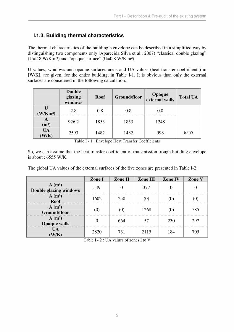
I.1.3. Building thermal characteristics
The thermal characteristics of the building’s envelope can be described in a simplified way by
distinguishing two components only (Aparecida Silva et al., 2007) “classical double glazing”
(U=2.8 W/K.m²) and “opaque surface” (U=0.8 W/K.m²).
U values, windows and opaque surfaces areas and UA values (heat transfer coefficients) in
[W/K], are given, for the entire building, in Table I-1. It is obvious than only the external
surfaces are considered in the following calculation.
Double
glazing
windows
Roof Ground/floor Opaque
external walls Total UA
U
(W/Km²) 2.8 0.8 0.8 0.8
A
(m²) 926.2 1853 1853 1248
UA
(W/K) 2593 1482 1482 998
6555
Table I - 1 : Envelope Heat Transfer Coefficients
So, we can assume that the heat transfer coefficient of transmission trough building envelope
is about : 6555 W/K.
The global UA values of the external surfaces of the five zones are presented in Table I-2:
Zone I Zone II Zone III Zone IV Zone V
A (m²)
Double glazing windows 549 0 377 0 0
A (m²)
Roof 1602 250 (0) (0) (0)
A (m²)
Ground/floor (0) (0) 1268 (0) 585
A (m²)
Opaque walls 0 664 57 230 297
UA
(W/K) 2820 731 2115 184 705
Table I - 2 : UA values of zones I to V
Part I – Description & Pre-audit of the existing system
6
I.2. Air Conditioning System
I.2.1. Offices Floor
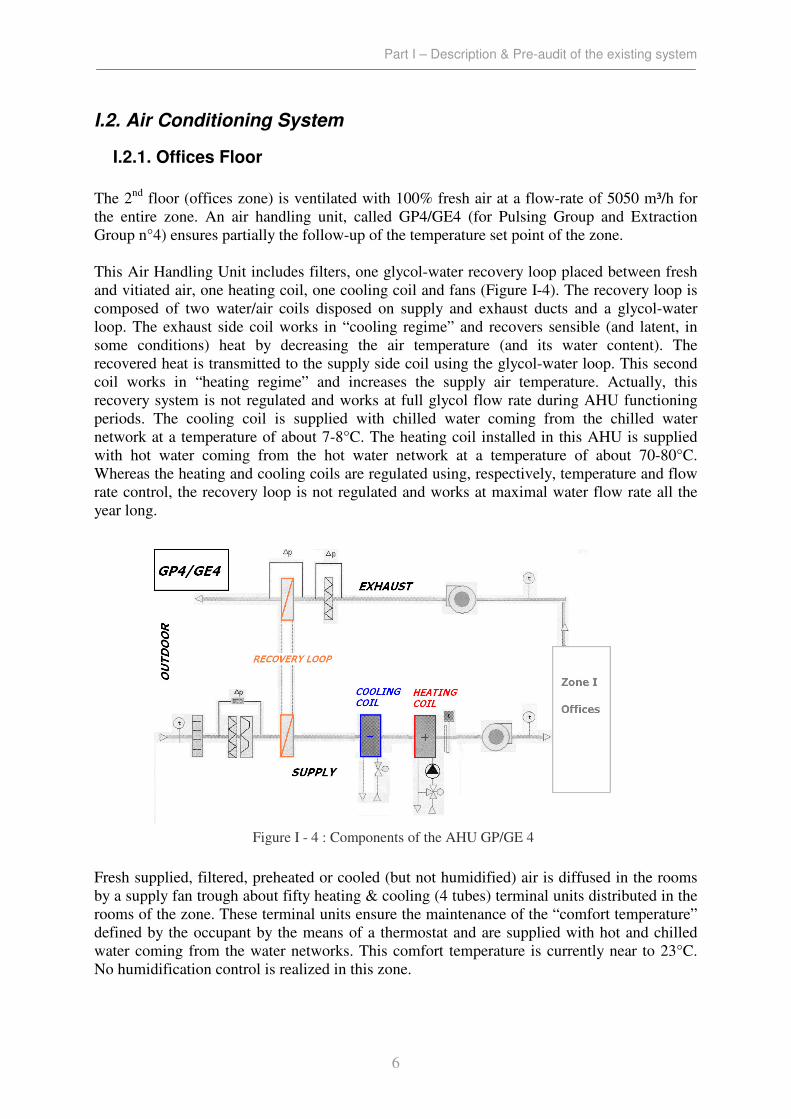
The 2nd
floor (offices zone) is ventilated with 100% fresh air at a flow-rate of 5050 m³/h for
the entire zone. An air handling unit, called GP4/GE4 (for Pulsing Group and Extraction
Group n°4) ensures partially the follow-up of the temperature set point of the zone.
This Air Handling Unit includes filters, one glycol-water recovery loop placed between fresh
and vitiated air, one heating coil, one cooling coil and fans (Figure I-4). The recovery loop is
composed of two water/air coils disposed on supply and exhaust ducts and a glycol-water
loop. The exhaust side coil works in “cooling regime” and recovers sensible (and latent, in
some conditions) heat by decreasing the air temperature (and its water content). The
recovered heat is transmitted to the supply side coil using the glycol-water loop. This second
coil works in “heating regime” and increases the supply air temperature. Actually, this
recovery system is not regulated and works at full glycol flow rate during AHU functioning
periods. The cooling coil is supplied with chilled water coming from the chilled water
network at a temperature of about 7-8°C. The heating coil installed in this AHU is supplied
with hot water coming from the hot water network at a temperature of about 70-80°C.
Whereas the heating and cooling coils are regulated using, respectively, temperature and flow
rate control, the recovery loop is not regulated and works at maximal water flow rate all the
year long.
Fresh supplied, filtered, preheated or cooled (but not humidified) air is diffused in the rooms
by a supply fan trough about fifty heating & cooling (4 tubes) terminal units distributed in the
rooms of the zone. These terminal units ensure the maintenance of the “comfort temperature”
defined by the occupant by the means of a thermostat and are supplied with hot and chilled
water coming from the water networks. This comfort temperature is currently near to 23°C.
No humidification control is realized in this zone.
Figure I - 4 : Components of the AHU GP/GE 4

Part I – Description & Pre-audit of the existing system
7
In small rooms, like offices, supplied air is diffused only trough the terminal units at a flow
rate of about 60 m³/h and extracted by an unique extraction orifice at a flow rate of 60m³/h.
Larger rooms, like small meeting rooms, are fed in fresh air trough the terminal unit and
trough additional air supply diffusers. The global extraction of vitiated air is made at a flow
rate of 3800 m³/h for the entire zone. The overpressure in the zone prevents any air
infiltration.
An additional AHU, called GP5, works in closed loop (with 100% recirculated air) and
ensures the conditioning of the large central open space. This group works at a flow rate of
about 5000 m³/h and includes a filter, a heating coil, a cooling coil and a fan.
The control strategy is similar to the other AHU (GP/GE4) and is charged to maintain the set-
point temperature in the zone.
Several types of terminal units are installed. Each device has five different working speeds
(characterized by 5 different air flow rates) but are similar in their structure (As built File,
2003). Installed Terminal Units (TU) characteristics are presented in Table I-3
Terminal Unit model TU size 3 TU size 5 TU size 6
Type Cooling&Heating
4 pipes
Cooling&Heating
4 pipes
Cooling&Heating
4 pipes
number 40 6 2
location offices Meeting rooms Meeting rooms
Air flow rates (m³/h) 180-280-410-575-750 210-320-465-670-960 210-325-475-675-975
Heating Power (kW) 1.9-2.6-3.4-4.1-4.6 2.3-3.1-4.0-5.0-6.0 2.4-3.4-4.4-5.5-6.7
Cooling Power (kW) 1.5-2.1-2.7-3.3-3.9 1.5-2.2-3.0-3.7-4.5 1.9-2.7-3.6-4.5-5.7
Table I – 3 : Terminal Units Characteristics
Heating and cooling powers are given in nominal conditions but correction factors are also
given by the manufacturer to allow the calculation of actual heating and cooling powers, as
function of working conditions.
The offices are occupied by about 70 people between 8:00 and 17:00, five days per week. The
zone is ventilated using the air handling unit between 6:00 and 20:00 five days per week too.
Terminal units ensure the set point temperature follow-up during the same period but are used
for a “re-starting” on Sunday evening between 15:00 and 20:00.
Figure I - 5 : Typical Terminal Unit Figure I - 6 : Components of the AHU GP5
Part I – Description & Pre-audit of the existing system
8
The first floor (technical room) is occupied only by a little maintenance team between 8:00
and 17:00 and is not conditioned. The high and constant temperature of the zone is only due
to the heat loss of the different components of the HVAC installation (Air Handling Units,
ducts, pipes…etc).
I.2.2. Laboratories Floor
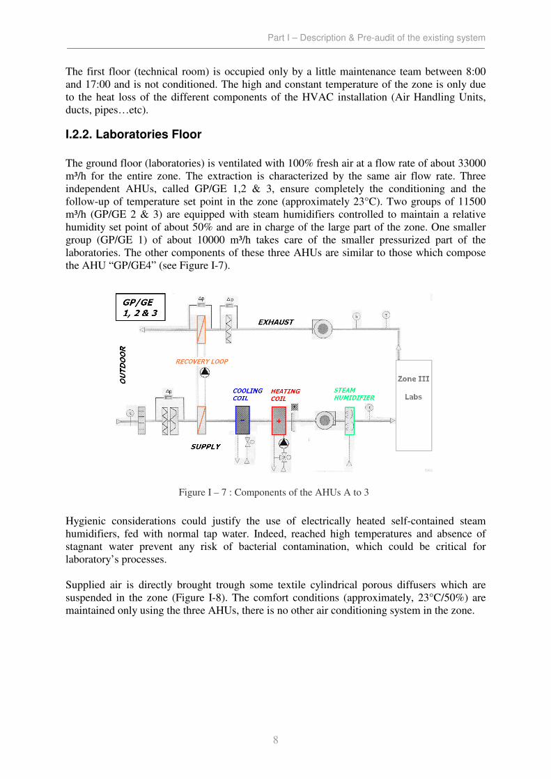
The ground floor (laboratories) is ventilated with 100% fresh air at a flow rate of about 33000
m³/h for the entire zone. The extraction is characterized by the same air flow rate. Three
independent AHUs, called GP/GE 1,2 & 3, ensure completely the conditioning and the
follow-up of temperature set point in the zone (approximately 23°C). Two groups of 11500
m³/h (GP/GE 2 & 3) are equipped with steam humidifiers controlled to maintain a relative
humidity set point of about 50% and are in charge of the large part of the zone. One smaller
group (GP/GE 1) of about 10000 m³/h takes care of the smaller pressurized part of the
laboratories. The other components of these three AHUs are similar to those which compose
the AHU “GP/GE4” (see Figure I-7).
Hygienic considerations could justify the use of electrically heated self-contained steam
humidifiers, fed with normal tap water. Indeed, reached high temperatures and absence of
stagnant water prevent any risk of bacterial contamination, which could be critical for
laboratory’s processes.
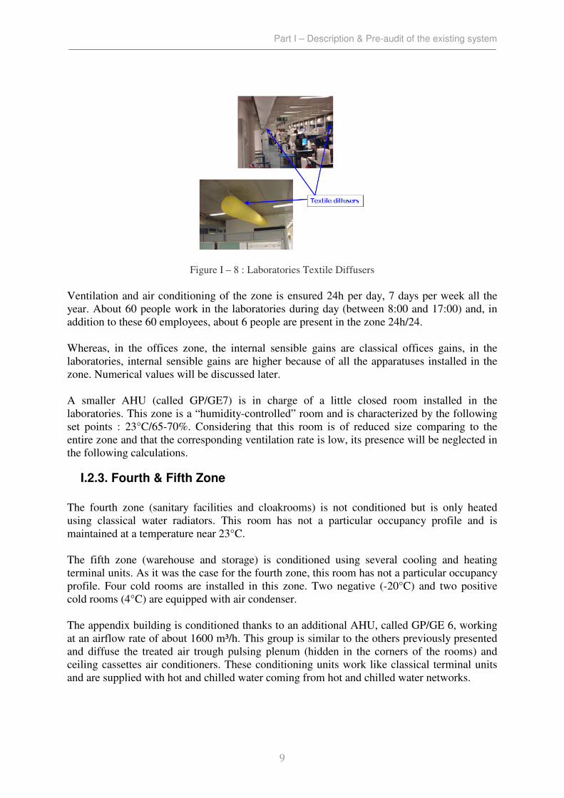
Supplied air is directly brought trough some textile cylindrical porous diffusers which are
suspended in the zone (Figure I-8). The comfort conditions (approximately, 23°C/50%) are
maintained only using the three AHUs, there is no other air conditioning system in the zone.
Figure I – 7 : Components of the AHUs A to 3
Part I – Description & Pre-audit of the existing system
9
Ventilation and air conditioning of the zone is ensured 24h per day, 7 days per week all the
year. About 60 people work in the laboratories during day (between 8:00 and 17:00) and, in
addition to these 60 employees, about 6 people are present in the zone 24h/24.
Whereas, in the offices zone, the internal sensible gains are classical offices gains, in the
laboratories, internal sensible gains are higher because of all the apparatuses installed in the
zone. Numerical values will be discussed later.
A smaller AHU (called GP/GE7) is in charge of a little closed room installed in the
laboratories. This zone is a “humidity-controlled” room and is characterized by the following
set points : 23°C/65-70%. Considering that this room is of reduced size comparing to the
entire zone and that the corresponding ventilation rate is low, its presence will be neglected in
the following calculations.
I.2.3. Fourth & Fifth Zone
The fourth zone (sanitary facilities and cloakrooms) is not conditioned but is only heated
using classical water radiators. This room has not a particular occupancy profile and is
maintained at a temperature near 23°C.
The fifth zone (warehouse and storage) is conditioned using several cooling and heating
terminal units. As it was the case for the fourth zone, this room has not a particular occupancy
profile. Four cold rooms are installed in this zone. Two negative (-20°C) and two positive
cold rooms (4°C) are equipped with air condenser.
The appendix building is conditioned thanks to an additional AHU, called GP/GE 6, working
at an airflow rate of about 1600 m³/h. This group is similar to the others previously presented
and diffuse the treated air trough pulsing plenum (hidden in the corners of the rooms) and
ceiling cassettes air conditioners. These conditioning units work like classical terminal units
and are supplied with hot and chilled water coming from hot and chilled water networks.
Figure I – 8 : Laboratories Textile Diffusers

Part I – Description & Pre-audit of the existing system
10
I.3. Refrigeration & Heating Plant
The installed power plant is composed of two recent condensing boilers and one air-cooled
chiller. Theses elements are installed in the central equipment room of the building (1st floor).
I.3.1. Heat Production
The heat production is ensured by two high efficiency gas condensing boilers of 300 kW each
(Figure I-9). These boilers supply the hot water network with water at a temperature of about
70-80°C and an efficiency of about 90% (based on HHV) in full load conditions. Of course, at
this temperature regime, the boilers do not function in condensing mode.
I.3.2. Cold Production
An air condenser chiller (Figure I-10) ensures the production of chilled water at a temperature
of 7-8°C for the whole building. The chilled water is used to supply the different cooling coils
of the HVAC system (AHU’s cooling coils and TU’s cooling coils).
This chiller is characterized by a nominal (12/7°C entering/leaving evaporator temperatures;
35°c ambient temperature) cooling capacity of about 399,1 kW. The corresponding power
demand (compressors only) is about 139,3 kW. The cooling of the condenser is ensured by
eight fans of about 780W each (electrical power) which brew about 99000 m³/h in nominal
conditions. The global nominal EER (eq. I.3.1) is about 2,75. The used refrigerant is
HFC407C.
fansWscompressorW
evaporatorQglobalERE
&&
&
+
= (I.3.1)
Figure I – 9 : Gas Condensing Boiler
Figure I – 10 : Air Cooled Chiller

Part I – Description & Pre-audit of the existing system
11
I.4. Water Distribution Network
As it has been said, hot water production is ensured by two condensing boilers disposed in
parallel. Four main pumps ensure the circulation of the hot water in the hot water network
(Table I-4). The first pump (C1) fed the heating coils of the air handling units and the second
(C2), the heating coils of the terminal units. The third pump (C3) ensures the supplying of
radiators. The fourth pump ensures the circulation in the (sanitary) hot water tank. The third
pump is not taken into account in our calculation because the radiators that they supply are
not in the modelled zones (but in zone IV). Not knowing the rate of demand for sanitary hot
water, hot water tank and its pump are not integrated in the calculations. So, only the pumps
C1 and C2 will be taken into account in the calculations. A simplified scheme of the hot water
networks is presented in Figure I-11.
Circuit Number Flow Rate
[m³/h]
Manometric Height
[m]
Efficiency
[%]
Electrical
Power [W]
C1 1 16.9 2.3 22 500
C2 1 7.7 5 31 350
C3 1 2.95 3.8 17 180
C4 1 2.5 1.8 13 100 Table I - 4 : Hot Water Network Pumps
Figure I – 11 : Hot Water Network Scheme

Part I – Description & Pre-audit of the existing system
12
Three pumps are used for the distribution of chilled water (Table I-5). The first pump (F1) fed
the cooling coils of the air handling units and the second (F2), the cooling coils of the
terminal units. The third pump (PRIM) is in charge of the primary chilled water network and
ensures the water circulation in the evaporator. These pumps are not equipped with inverters,
so, we can suppose that they work in nominal conditions as soon as there is a cooling demand
in the building. Vanes ensure regulation of the chilled water network.
A simplified scheme of the hot water networks is presented in Figure I-12 .
Circuit Number Flow Rate
[m³/h]
Manometric
Height [m]
Efficiency
[%]
Electrical
Power [W]
F1 1 49 7 56 1700
F2 1 25.4 6 42 1000
PRIM 1 70 5.5 36 3300 Table I - 5 : Chilled Water Network Pumps
Figure I – 12 : Chiller Water Network Scheme

Part I – Description & Pre-audit of the existing system
13
I.5. Pre-audit of the Installation
I.5.1. Electricity & Gas Consumptions
The audit of an existing HVAC system consists in analysing the available information about
actual energy consumptions and global performances. In the following pre-audit, only directly
available information (visual verifications, as-built records analysis, operating costs and
consumptions, short and limited measurements) and very simple calculation will be used to
analyse the installation and identify the most attractive retrofit opportunities (Lebrun et al.,
2006a; Aparecida Silva et al.,2007).
After having regarded the building’s design and the HVAC system’s functioning, it’s time to
consider the available data as electrical and gas consumptions. As usually, monthly records of
electricity and gas energy consumptions are available. The electrical consumption between
January 2005 and July 2006 is plotted in Figure I-13. It appears that the average electricity
consumption for this period is floating around 130000 kWh/month. It seems difficult to
highlight a possible seasonal effect but the effect of steam humidification can be noted.
Indeed, winter month’s consumptions are greater than summer month’s consumptions. This
observation can be explained by the fact that (winter) steam humidification is more
consuming than (summer) cooling and will be better highlighted in the following figures.
Figure I – 13 : Electrical Consumption – Jan05 to July06
Part I – Description & Pre-audit of the existing system
14
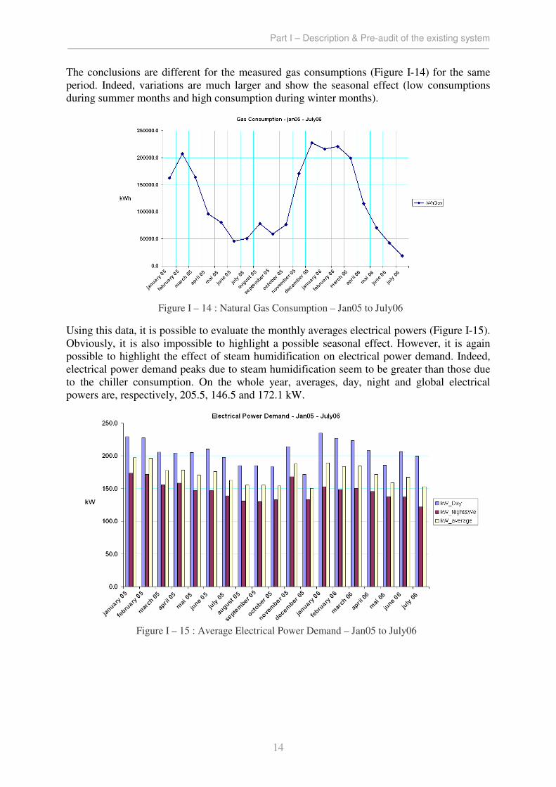
The conclusions are different for the measured gas consumptions (Figure I-14) for the same
period. Indeed, variations are much larger and show the seasonal effect (low consumptions
during summer months and high consumption during winter months).
Using this data, it is possible to evaluate the monthly averages electrical powers (Figure I-15).
Obviously, it is also impossible to highlight a possible seasonal effect. However, it is again
possible to highlight the effect of steam humidification on electrical power demand. Indeed,
electrical power demand peaks due to steam humidification seem to be greater than those due
to the chiller consumption. On the whole year, averages, day, night and global electrical
powers are, respectively, 205.5, 146.5 and 172.1 kW.
Figure I – 14 : Natural Gas Consumption – Jan05 to July06
Figure I – 15 : Average Electrical Power Demand – Jan05 to July06
Part I – Description & Pre-audit of the existing system
15
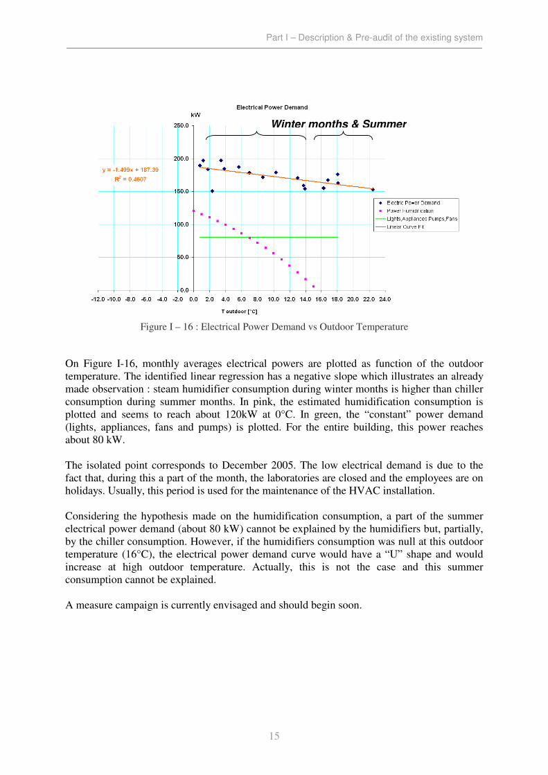
On Figure I-16, monthly averages electrical powers are plotted as function of the outdoor
temperature. The identified linear regression has a negative slope which illustrates an already
made observation : steam humidifier consumption during winter months is higher than chiller
consumption during summer months. In pink, the estimated humidification consumption is
plotted and seems to reach about 120kW at 0°C. In green, the “constant” power demand
(lights, appliances, fans and pumps) is plotted. For the entire building, this power reaches
about 80 kW.
The isolated point corresponds to December 2005. The low electrical demand is due to the
fact that, during this a part of the month, the laboratories are closed and the employees are on
holidays. Usually, this period is used for the maintenance of the HVAC installation.
Considering the hypothesis made on the humidification consumption, a part of the summer
electrical power demand (about 80 kW) cannot be explained by the humidifiers but, partially,
by the chiller consumption. However, if the humidifiers consumption was null at this outdoor
temperature (16°C), the electrical power demand curve would have a “U” shape and would
increase at high outdoor temperature. Actually, this is not the case and this summer
consumption cannot be explained.
A measure campaign is currently envisaged and should begin soon.
Winter months & Summer
Figure I – 16 : Electrical Power Demand vs Outdoor Temperature

Part I – Description & Pre-audit of the existing system
16
Figure I-17 shows the measured electrical power demand due to the coldrooms chillers. Two
average values can be computed : a “week average value” corresponding to the occupancy
periods during which the coldrooms are opened a few times per day and a “weekend average
value” during which the coldrooms stay closed all the time.
Figure I – 17 : Coldrooms Electrical Power Demand

Part I – Description & Pre-audit of the existing system
17
I.5.2. Thermal Signature
In the frame of an auditing project, the thermal signature is the distribution of the fuel/gas
power defined in monthly average (between January 2005 and July 2006 in our case), as
function of the external dry bulb temperature (Lebrun et al., 2006a; Aparecida Silva et
al.,2007). Figure I-18 gives this thermal signature for the concerned building. It gives a good
correlation factor (0.94) and allows a meaningful linear regression to be identified. Its
equation is given on Figure I-18. The slope of this law (-14.05 kW/K) should correspond to
the global average heat transfer coefficient of the building.
Using the building thermal characteristics and the building envelope’s heat transfer coefficient
(UA = K = 6.555 [kW/K]), it is possible to retrieve the “average heat transfer coefficient”
given by thermal signature correlation (Aparecida Silva et al., 2007).
Considering a ventilation air flow rate of about 38000 m³/h for the whole building (10000
m³/h for GP1, 11500 m³/h for GP2 & GP3 and about 5000 m³/h for GP5, see HVAC system
description), the mechanical ventilation heat transfer coefficient (or thermal capacity flow
rate) is calculated as follows :
Figure I – 18 : Building’s Thermal Signature

Part I – Description & Pre-audit of the existing system
18
The calculation gives :
Considering that, in nominal conditions, recovery loops have an efficiency of about 42%
(given in manufacturer data), we can compute the “heat recovery potential” :
This means that the net ventilation heating demand is about : 12.73 – 5.7 = 7.03 kW/K
The global heating demand of the building can be estimated by adding transmission (trough
building’s envelope) and ventilation terms :
Then, the total heating demand heat transfer coefficient is about : 13.585 [kW/K]. Note that
this value has not been modified to take ventilation intermittency into account. Indeed, the
greatest part of the total ventilation flow rate (39600 m³/h) is due to the ventilation of the
laboratories (33000 m³/h, 24h/day, 7d/week).
The value obtained thanks to this rough calculation is in fair agreement with the slope (14.05
[kW/K]) of the building “thermal signature” as shown in Figure I-18. This result is very
important and allows us to affirm that the gas consumption can be explained by the building’s
heating demand. Moreover, these results are encouraging and confirm the hypotheses made
on the heat transfer coefficients.
Part I – Description & Pre-audit of the existing system
19
I.6. Conclusions
In spite of recent character of the installation and its potential high efficiency, gas and
electrical consumptions are important and the source of high costs (and CO2 emissions).
An important part of these costs is due to the steam humidification systems. Indeed, these
apparatuses are very hygienic and characterized by their simplicity and facility of use but are
also great consumer of electrical energy. However, in the case of laboratories, the use of
steam humidification instead of adiabatic humidification can be justified. A first proposal
could be to verify if the needs for humidification and these high temperature and humidity set
points (23°C/50%) are justified.
Whereas the winter electrical consumption is quite well explained (by constant consumptions
and steam humidifiers consumptions), at the moment, it is not possible to affirm that the
summer electrical consumption is totally due to the chiller. The modelling of the installation
will be useful to clear up this specific point.
As the thermal signature shown it, the gas consumption can be explained by the heating
demand of the building. Indeed, the thermal signature coefficient corresponds to the heat
transfer coefficient of the building’s envelope.
Part I – Description & Pre-audit of the existing system
20
I.7. Retrofit Opportunities
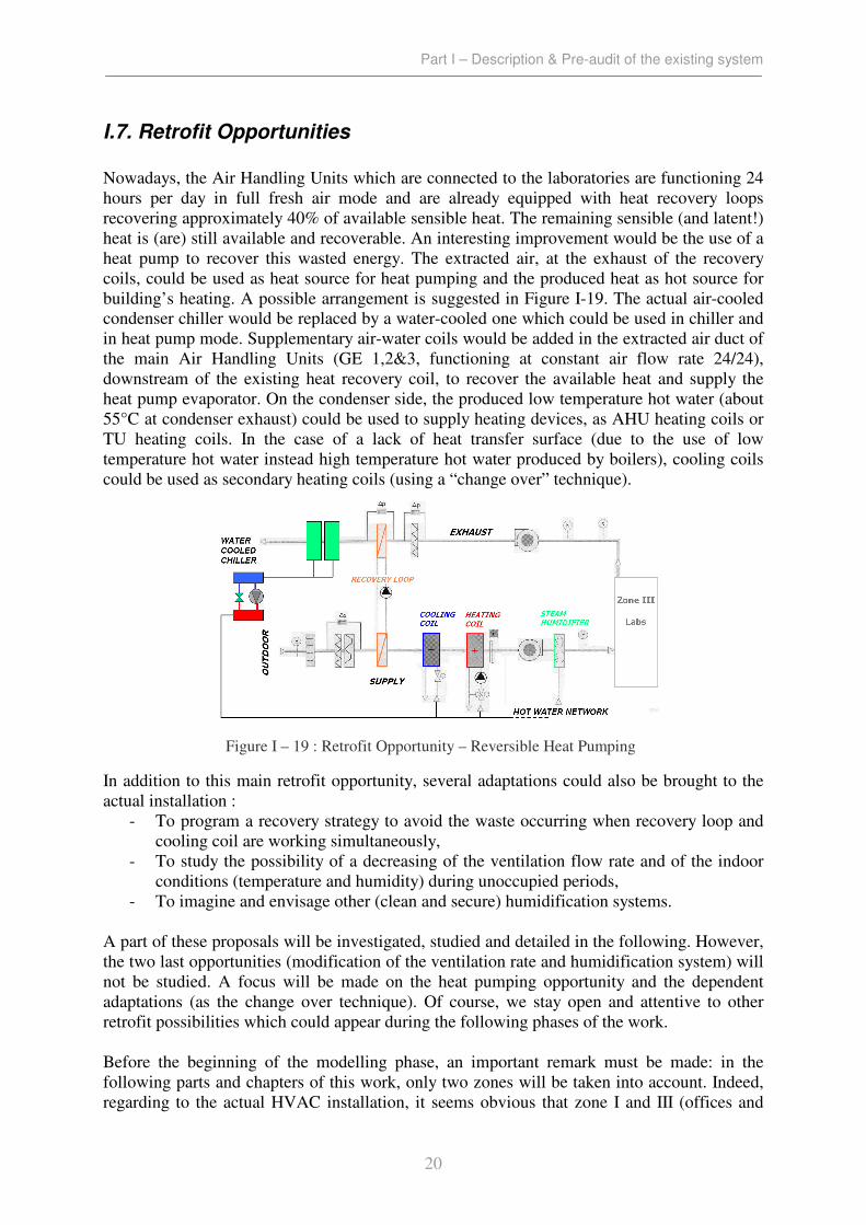
Nowadays, the Air Handling Units which are connected to the laboratories are functioning 24
hours per day in full fresh air mode and are already equipped with heat recovery loops
recovering approximately 40% of available sensible heat. The remaining sensible (and latent!)
heat is (are) still available and recoverable. An interesting improvement would be the use of a
heat pump to recover this wasted energy. The extracted air, at the exhaust of the recovery
coils, could be used as heat source for heat pumping and the produced heat as hot source for
building’s heating. A possible arrangement is suggested in Figure I-19. The actual air-cooled
condenser chiller would be replaced by a water-cooled one which could be used in chiller and
in heat pump mode. Supplementary air-water coils would be added in the extracted air duct of
the main Air Handling Units (GE 1,2&3, functioning at constant air flow rate 24/24),
downstream of the existing heat recovery coil, to recover the available heat and supply the
heat pump evaporator. On the condenser side, the produced low temperature hot water (about
55°C at condenser exhaust) could be used to supply heating devices, as AHU heating coils or
TU heating coils. In the case of a lack of heat transfer surface (due to the use of low
temperature hot water instead high temperature hot water produced by boilers), cooling coils
could be used as secondary heating coils (using a “change over” technique).
In addition to this main retrofit opportunity, several adaptations could also be brought to the
actual installation :
- To program a recovery strategy to avoid the waste occurring when recovery loop and
cooling coil are working simultaneously,
- To study the possibility of a decreasing of the ventilation flow rate and of the indoor
conditions (temperature and humidity) during unoccupied periods,
- To imagine and envisage other (clean and secure) humidification systems.
A part of these proposals will be investigated, studied and detailed in the following. However,
the two last opportunities (modification of the ventilation rate and humidification system) will
not be studied. A focus will be made on the heat pumping opportunity and the dependent
adaptations (as the change over technique). Of course, we stay open and attentive to other
retrofit possibilities which could appear during the following phases of the work.
Before the beginning of the modelling phase, an important remark must be made: in the
following parts and chapters of this work, only two zones will be taken into account. Indeed,
regarding to the actual HVAC installation, it seems obvious that zone I and III (offices and
Figure I – 19 : Retrofit Opportunity – Reversible Heat Pumping

Part I – Description & Pre-audit of the existing system
21
laboratories) are the zones in charge of the main part of the consumptions due to the HVAC
system. On one hand, laboratories and offices are characterized by an important HVAC
system, composed of large air handling units and a high number of terminal units. On the
other hand, the remaining zones are equipped with only some radiators (about 6) and a small
air handling unit (GP/GE 6). Moreover, the whole building is ventilated (with full fresh air) at
a rate of about 39600 m³/h when zones I and III totalise 38000 m³/h. All theses observations
justify the fact that, in the following work, only zones I and III will be taken into account. The
other zones will be studied later, in the frame of the IEA Annex48 project. Of course, only the
equipments corresponding to the studied zones will be taken into account in the calculations.

Part II – Modelling of the installation
22
PART II : MODELLING OF THE INSTALLATION

Part II – Modelling of the installation
23
II.1. Aim & Philosophy of The Modelling Phase
While, in a pre-audit procedure, the identification of the building heating & cooling demands
is not envisaged (heat/cool counters are not often installed in buildings), the calculation of
theoretical demands and corresponding energy consumptions appears logically at the start of a
feasibility calculation and detailed study of retrofit opportunities.
Considering the number of parameters and influences which are involved in this type of
calculation, it seems rational to run simulation model rather than very global and hypothetical
weather indexes (similar to heating degree-days). For this targeted work, simulation models
are required that are sufficiently reliable, accurate and robust.
The level of detail required for each calculation can be very different. For heating
calculations, the major issues are a correct description of the building envelope and an
accurate evaluation of the air renewal. For cooling calculations, the fenestration area and
orientation, the level and distribution of the internal gains, the ventilation rates, and the
geographical location appear as critical issues. Most of these issues are explicitly taken into
account in the developed models.
The presented model could be divided in two main parts :
- a dynamic building model,
- a static HVAC system model.
The first part of the global model ensures the calculation of the heating and cooling loads
whereas the second part (HVAC system model) involves moving from building demands to
system energy consumptions.
In both situations, the issue is to define the optimal level of detail of the model in relationship
to the amount of information collected during the pre-auditing phase and the required qualities
of the model. To this end, only one building model will be used in the following work but
three types of models will be developed for the HVAC system components:
- complete, validated, detailed and accurate models (called “mother models”), used to
compute components characteristics and properties (basing on manufacturer data)
- simplified, robust and more easy-to-use models (called “daughter models”), using the
previously defined characteristics to run simulations,
- Simplified, robust and easy to tune models (called “orphan models”), directly tuned
using manufacturer data.
Most of these models have already been developed, validated and used in University of Liège
(André et al., 2006a; André et al., 2006b) in the frame of the following research projects :
- IEA ECBCS Annex 10
- ASHRAE Primary Toolkit
- IEA ECBCS Annex 40
- IEA ECBCS Annex 43
- AUDITAC
- IEA ECBCS Annex 48
Part II – Modelling of the installation
24
II.2. Building Model
The following building model has been developed as a “benchmarking – auditing” tool in
University of Liège (André, Lebrun et al., 2006a) and implemented on “EES” (Engineering
Equation Software, © F-Chart Software).
Obviously, the simulation model includes realistic and physical considerations, as :
- building (static and dynamic) behaviour,
- weather and occupancy loads,
- solar exposure and orientations,
- characteristics of materials composing the building’s envelope.
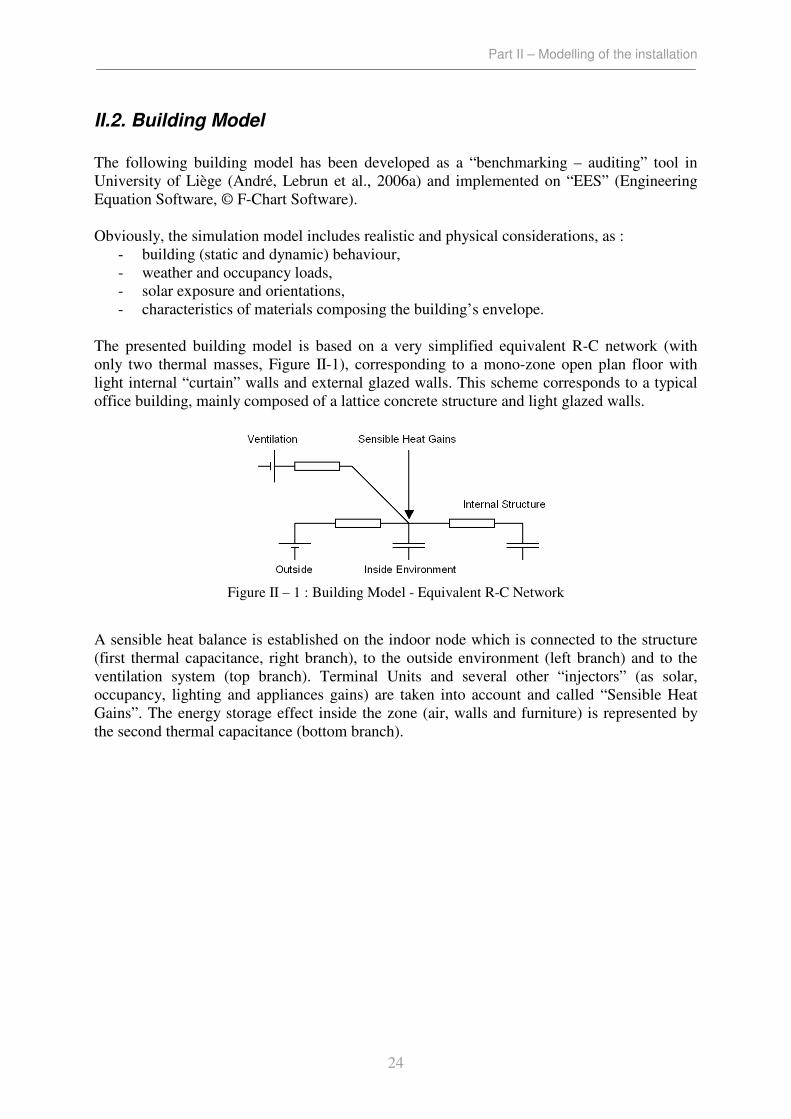
The presented building model is based on a very simplified equivalent R-C network (with
only two thermal masses, Figure II-1), corresponding to a mono-zone open plan floor with
light internal “curtain” walls and external glazed walls. This scheme corresponds to a typical
office building, mainly composed of a lattice concrete structure and light glazed walls.
A sensible heat balance is established on the indoor node which is connected to the structure
(first thermal capacitance, right branch), to the outside environment (left branch) and to the
ventilation system (top branch). Terminal Units and several other “injectors” (as solar,
occupancy, lighting and appliances gains) are taken into account and called “Sensible Heat
Gains”. The energy storage effect inside the zone (air, walls and furniture) is represented by
the second thermal capacitance (bottom branch).
Figure II – 1 : Building Model - Equivalent R-C Network
Part II – Modelling of the installation
25
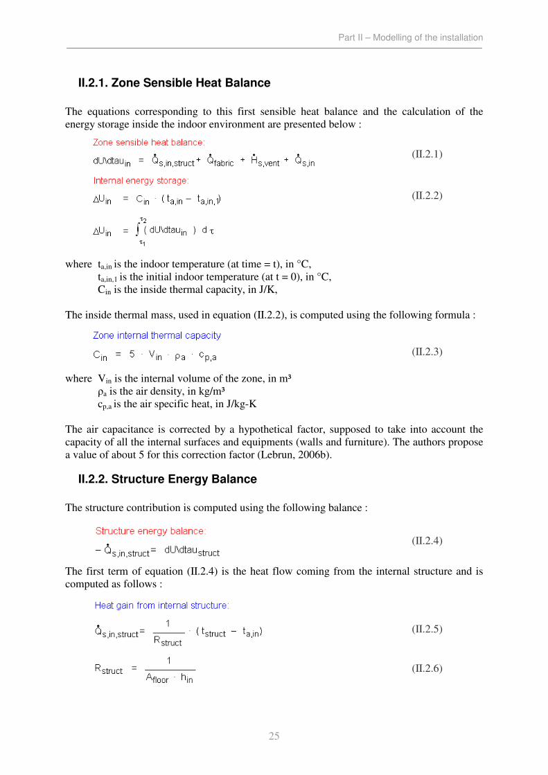
II.2.1. Zone Sensible Heat Balance
The equations corresponding to this first sensible heat balance and the calculation of the
energy storage inside the indoor environment are presented below :
where ta,in is the indoor temperature (at time = t), in °C,
ta,in,1 is the initial indoor temperature (at t = 0), in °C,
Cin is the inside thermal capacity, in J/K,
The inside thermal mass, used in equation (II.2.2), is computed using the following formula :
where Vin is the internal volume of the zone, in m³
ρa is the air density, in kg/m³
cp,a is the air specific heat, in J/kg-K
The air capacitance is corrected by a hypothetical factor, supposed to take into account the
capacity of all the internal surfaces and equipments (walls and furniture). The authors propose
a value of about 5 for this correction factor (Lebrun, 2006b).
II.2.2. Structure Energy Balance
The structure contribution is computed using the following balance :
The first term of equation (II.2.4) is the heat flow coming from the internal structure and is
computed as follows :
(II.2.1)
(II.2.2)
(II.2.3)
(II.2.4)
(II.2.5)
(II.2.6)
Part II – Modelling of the installation
26
where Rstruct is the thermal resistance corresponding to the global exchange (convective and
radiative) between the ambiance and the structure, in K/W,
tstruct is the structure temperature (at time = t), in °C,
Afloor is the floor surface, in m²,
hin is the inside global exchange coefficient, in W/m²-K.
The second term appearing in equation (II.2.4) is the energy stored in the structure :
where Cstruct is the structure thermal capacity, in J/K,
tstruct,1 is the initial structure temperature (at t = 0), in °C,
efloor is the floor thickness, in m,
rhofloor is the floor density, in kg/m³,
cfloor is the floor specific heat, in J/kg-K.
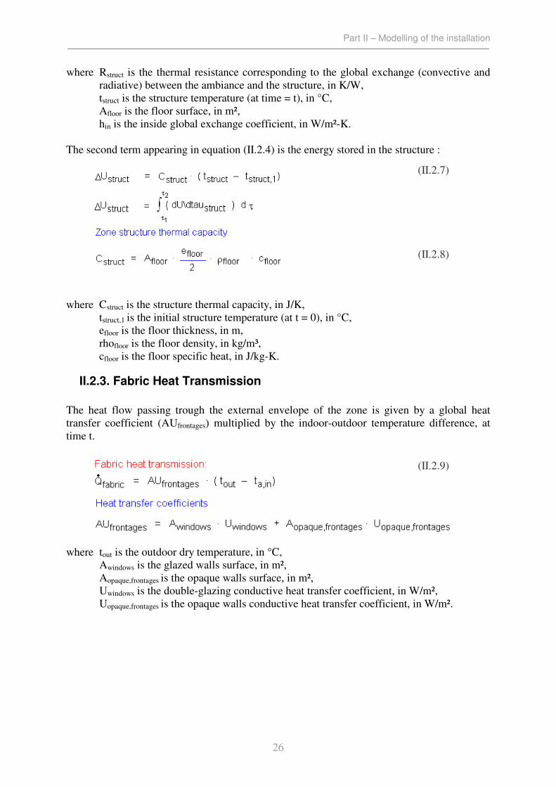
II.2.3. Fabric Heat Transmission
The heat flow passing trough the external envelope of the zone is given by a global heat
transfer coefficient (AUfrontages) multiplied by the indoor-outdoor temperature difference, at
time t.
where tout is the outdoor dry temperature, in °C,
Awindows is the glazed walls surface, in m²,
Aopaque,frontages is the opaque walls surface, in m²,
Uwindows is the double-glazing conductive heat transfer coefficient, in W/m²,
Uopaque,frontages is the opaque walls conductive heat transfer coefficient, in W/m².
(II.2.7)
(II.2.8)
(II.2.9)

Part II – Modelling of the installation
27
II.2.4. Ventilation Enthalpy Flow rate
The enthalpy flow rate brought by pulsed and infiltrated airflow rates is given by :
where M& a,ex,supplyduct is the pulsed air mass flow rate, in kg/s,
cp,a is the air specific heat, in J/kg-K,
C& ex,supplyduct is the pulsed air specific heat flow rate, in J/K-s,
M& a,infiltr is the infiltrated air mass flow rate, in kg/s,
C& infiltr is the infiltrated air specific heat flow rate, in J/K-s.
II.2.5. Sensible Heat Gains
The equation (II.2.11) summarizes the different sensible heat gains (or “injectors”) which
have not been taken into account till now :
where Q& s,in is the global sensible heat gain in the zone, in W,
Q& s,occ is the sensible heat gain due to the occupancy, in W,
W& light is the heat gain due to the lighting, in W,
W& appl is the heat gain due to the appliances, in W,
Q& sun is the solar gain, in W,
Q& s,heating is the heating load provided by terminal units, in W,
Q& s,cooling is the cooling load provided by terminal units, in W.
These two last contributions are calculated using the terminal unit model described below.
The occupancy load is given by :
where Q& sensible\occupant is the sensible heat gain per occupant due to a moderately active office
work (ASHRAE, 2005), in W,
nocc is the number of occupants in the zone.
(II.2.10)
(II.2.11)

Part II – Modelling of the installation
28
Lighting and Appliances gains are computed as follows :
where W& light,max is the maximal heat gain due to the lighting, in W,
W& light,max\A,floor is the maximal heat gain due to the lighting per square meter of
surface, in W/m²,
W& appl,max is the maximal heat gain due to the installed appliances, in W,
W& appl,max\A,floor is the maximal heat gain due to the installed appliances per square
meter of surface, in W/m².
The solar gain, directly injected in the zone trough windows, is composed of three main
contributions :
- the direct radiation,
- the diffused radiation,
- the reflected radiation.
These three contributions are included in the following equation which enables the calculation
of a global radiation, called Isun, in W/m². A solar factor (SFwindows) globalises the reflection,
absorption and transmission factors of the double-glazing windows in one value.
Considering theses values, the solar heat gain is easily obtained :
The global radiation is obtained by adding the three contributions :
where Isun is the global radiation, in W/m²,
Idirect is the direct radiation reaching the vertical glazed surfaces, in W/m²,
Iglob is the global radiation reaching a horizontal surface of 1m², in W/m²,
Albedo is the reflective factor of the ground,
Idiff is the diffused radiation on a horizontal surface of 1m², in W/m².
The factors ½ are added because a vertical wall faces only half of the sky. The global and
diffuse radiations come directly from the meteorological data. The direct radiation is
calculated as follows :
Part II – Modelling of the installation
29
where Fwindows,South is the proportion of glazed surface South oriented, in m²/m²,
Fwindows,West is the proportion of glazed surface West oriented, in m²/m²,
Fwindows,East is the proportion of glazed surface East oriented, in m²/m²,
Fwindows,North is the proportion of glazed surface North oriented, in m²/m²,
Fwindows,shadow is the proportion of shadowed glazed surface, in m²/m²,
SIGMAFwindows is the sum of the previous factors, equal to 1, in m²/m²,
FSouth is the projection factor for a vertical south-facing wall,
FWest is the projection factor for a vertical west-facing wall,
FEast is the projection factor for a vertical east-facing wall,
FNorth is the projection factor for a vertical north-facing wall,
Projection factors are used to transform the radiation reaching a horizontal surface into the
radiation reaching a vertical wall. The F factor is a global projection factor which takes into
account the corresponding orientations (North, West, South and East). Glazed surfaces are
known and computed using the plans. Projection factors are available in the climate data file.
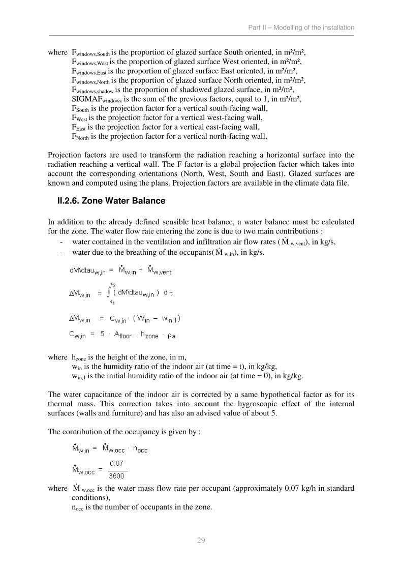
II.2.6. Zone Water Balance
In addition to the already defined sensible heat balance, a water balance must be calculated
for the zone. The water flow rate entering the zone is due to two main contributions :
- water contained in the ventilation and infiltration air flow rates ( M& w,vent), in kg/s,
- water due to the breathing of the occupants( M& w,in), in kg/s.
where hzone is the height of the zone, in m,
win is the humidity ratio of the indoor air (at time = t), in kg/kg,
win,1 is the initial humidity ratio of the indoor air (at time = 0), in kg/kg.
The water capacitance of the indoor air is corrected by a same hypothetical factor as for its
thermal mass. This correction takes into account the hygroscopic effect of the internal
surfaces (walls and furniture) and has also an advised value of about 5.
The contribution of the occupancy is given by :
where M& w,occ is the water mass flow rate per occupant (approximately 0.07 kg/h in standard
conditions),
nocc is the number of occupants in the zone.

Part II – Modelling of the installation
30
The contributions of the ventilation and the infiltration are given by :
where wex,supplyduct is the humidity ratio of the pulsed air, in kg/kg,
wout is the humidity ratio of the outdoor air, in kg/kg.
II.2.7. Building Model Parameters
The present model will be used to simulate the heating and cooling demands of the offices
and laboratories floors. The reason why only zones I and III will be taken into account in this
work has already been explained in the conclusion of the first part of this report.
To facilitate the modelling and computing work, the previously presented mono-zone building
model has been used as it is and has not been transformed in a multi-zone model. So, each
considered zone will be modelled and simulated independently. This fair and convenient
approximation could be justified by the fact that the two studied zone are quite independent
one of the other (Figure II-2). Indeed, the technical room (zone II, characterized by a quite
constant temperature) play the role of a “buffer zone” which prevents any influence between
the zones I and III.
The laboratories are also directly “in contact” with zone IV. However, considering the facts
that this fourth zone is characterized by a close temperature and that the air circulation
between these two zones is very low, the zone IV is taken into account as an isothermal
adjoining zone in the simulation of the laboratories.
.
Figure II – 2 : Cross Section of the Building

Part II – Modelling of the installation
31
The simulation parameters for the both zones are presented in Table II-1.
Units Laboratories Offices
Zone
Length m 65 82
Width m 19.5 19.5
height m 2.9 2.7
Structure
Floor thickness m 0.2 0.2
Floor Density kg/m³ 2000 2000
Floor Spec. Heat J/kg-K 850 850
Materials
Uwindows W/K-m² 2.8 2.8
SFwindows - 0.25 0.25
Uopaque W/K-m² 0.8 0.8
Exposure
albedo - 0.2 0.2
Fwin,South % 44 20
Fwin,West % 0 10
Fwin,North % 44 20
Fwin,East % 0 10
Fwin,shadow - 0 40
Equipments
Lighting W/m² 5 5
Appliances W/m² 25 5 Table II – 1 : Parameters of the Building Model
U values correspond to the values used in the pre-audit. The thermal signature previously
made has confirmed these hypotheses. Windows solar factor and albedo values are classical
mean values (Lebrun, 2006b). Exposure factors and equipments loads have been estimated
according to the actual geometry and installed appliances (As built File, 2003).
Once the studied zones are modelled, a simulation model must also be developed for the
complete HVAC system.
Part II – Modelling of the installation
32
II.3. HVAC System Model
As already said in the first part of this work, installed CAV (constant air volume) air handlers
generally include air-to-air direct recovery loops, hot water heating coils, chilled water
cooling coils, steam humidifiers and fans. In one zone (offices), classical heating & cooling
terminal units are installed to ensure a permanent comfort temperature. All of these
components will be now described and modelled.
Considering that the building model is a mono-zone model, all the models of the equipments
of a given type (air handling units, terminal units…etc) can be gathered in a “global” model.
Indeed, the different locations of the terminal units or of the air diffusers cannot be taken into
account in a simplified mono-zone building model, it is so totally useless to differentiate the
similar units. The global model is so composed of a mono-zone building model, a global air
handling unit model (gathering the characteristics of the different AHU which are in charge of
the zone) and a global terminal unit model (for the offices floor only). A last part of the model
concerns the calculation of electrical and gas consumptions (using chiller and boiler models)
and is only provided with cooling and heating demand previously calculated. These models
will be presented below.
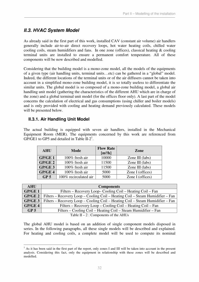
II.3.1. Air Handling Unit Model
The actual building is equipped with seven air handlers, installed in the Mechanical
Equipment Room (MER). The equipments concerned by this work are referenced from
GP/GE1 to GP5 and detailed in Table II-21.
AHU Mode Flow Rate
[m³/h] Zone
GP/GE 1 100% fresh air 10000 Zone III (labs)
GP/GE 2 100% fresh air 11500 Zone III (labs)
GP/GE 3 100% fresh air 11500 Zone III (labs)
GP/GE 4 100% fresh air 5000 Zone I (offices)
GP 5 100% recirculated air 5000 Zone I (offices)
AHU Components
GP/GE 1 Filters – Recovery Loop– Cooling Coil – Heating Coil – Fan
GP/GE 2 Filters – Recovery Loop – Cooling Coil – Heating Coil – Steam Humidifier – Fan
GP/GE 3 Filters – Recovery Loop – Cooling Coil – Heating Coil – Steam Humidifier – Fan
GP/GE 4 Filters – Recovery Loop – Cooling Coil – Heating Coil – Fan
GP 5 Filters – Cooling Coil – Heating Coil – Steam Humidifier – Fan Table II – 2 : Components of the AHUs
The global AHU model is based on an addition of single component models disposed in
series. In the following paragraphs, all these single models will be described and explained.
For heating and cooling coils, a complete model will be used to compute its nominal
1 As it has been said in the first part of the report, only zones I and III will be taken into account in the present
analysis. Considering this fact, only the equipment in relationship with these zones will be described and
modelled.
Part II – Modelling of the installation
33
characteristics. These characteristics will be used during simulations by a simplified (more
robust) model. The other models are “orphan”, but simple models.
II.3.1.1. Heating Coil Model
In the considered installation, aluminium fin&tube coils, fed with hot water coming from the
hot water network, are used to heat the air at the exhaust of the recovery coils. These devices
are regulated thanks to the supply hot water temperature (controlled using a mixing three-way
vane and a pump).
Complete “Mother” Model
Currently, (pre)heating coils are characterized by their heat transfer surface, composed of a
primary (tubes external surface) and a secondary (fins external surface) heat transfer surface.
The global heat transfer surface can be numerically represented by a global AU value of the
coil. The aim of this first mother model is to determine the nominal AU value of the coil,
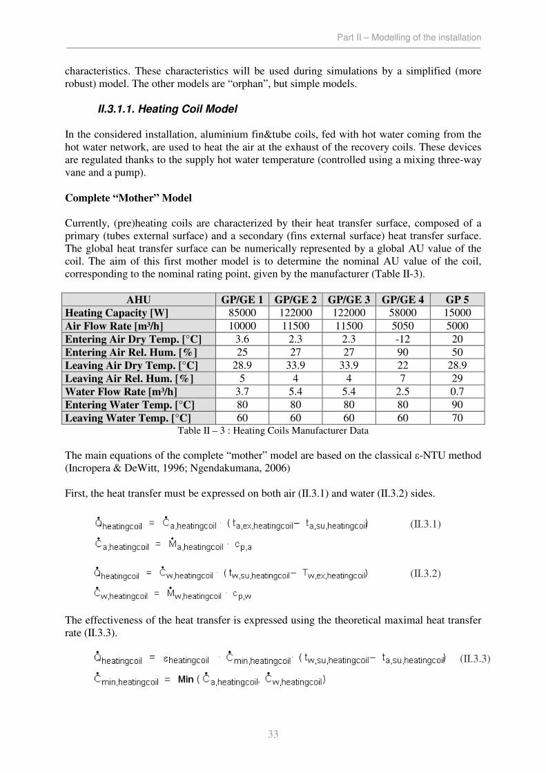
corresponding to the nominal rating point, given by the manufacturer (Table II-3).
AHU GP/GE 1 GP/GE 2 GP/GE 3 GP/GE 4 GP 5
Heating Capacity [W] 85000 122000 122000 58000 15000
Air Flow Rate [m³/h] 10000 11500 11500 5050 5000
Entering Air Dry Temp. [°C] 3.6 2.3 2.3 -12 20
Entering Air Rel. Hum. [%] 25 27 27 90 50
Leaving Air Dry Temp. [°C] 28.9 33.9 33.9 22 28.9
Leaving Air Rel. Hum. [%] 5 4 4 7 29
Water Flow Rate [m³/h] 3.7 5.4 5.4 2.5 0.7
Entering Water Temp. [°C] 80 80 80 80 90
Leaving Water Temp. [°C] 60 60 60 60 70 Table II – 3 : Heating Coils Manufacturer Data
The main equations of the complete “mother” model are based on the classical ε-NTU method
(Incropera & DeWitt, 1996; Ngendakumana, 2006)
First, the heat transfer must be expressed on both air (II.3.1) and water (II.3.2) sides.
The effectiveness of the heat transfer is expressed using the theoretical maximal heat transfer
rate (II.3.3).
(II.3.1)
(II.3.2)
(II.3.3)

Part II – Modelling of the installation
34
This effectiveness can be expressed as a function of the heat transfer coefficient AUheatingcoil,
using the following formula (II.3.4).
The formula (II.3.4) corresponds to a counter-flow heat exchanger. In spite of the particular
conception of heating coils, this approximation can be made for coils with more than 3 rows
of tubes.
The obtained AU value also corresponds to the reverse of the total thermal resistance which
exists between the air and the water flow rates. This total thermal resistance is also equivalent
to three resistances disposed in series : the convective resistance on the airside, the conduction
resistance of the metal and the convective resistance on the waterside.
The present model is implemented on “EES” and used for the five considered coils (Figure II-
3). Specific heat and densities are computed using the property functions implemented in
“EES” with air and water mean temperatures and at a standard atmospheric pressure of about
101325 Pa. Results obtained for the five runs are presented in Table II-4.
(II.3.4)
Figure II – 3 : Block Diagram Representation of the
Heating Coil Model

Part II – Modelling of the installation
35
AHU Coil AU value
[W/K] Coil Effectiveness
Heating
Capacity [W]
Leaving Air
Temperature [°C]
GP/GE 1 1557 0.3225 84149 28.24
GP/GE 2 2374 0.4054 122813 33.8
GP/GE 3 2374 0.4054 122813 33.8
GP/GE 4 861 0.3434 56858 19.59
GP/GE 5 287.9 0.2857 15851 29.55 Table II – 4 : Heating Coils Computed Characteristics
By comparing these results to the values given by the manufacturer (Table II-3), absolute and
relative errors can be computed. Thus, leaving air temperature is calculated with an average
absolute accuracy of about 0.7 °C. The heating capacity is computed with an average absolute
accuracy of about 2%. Considering the simplicity and the fact that this model is currently
used, no validation work will be realized for this model.
Simplified “Daughter” Model
To avoid difficult calculations and convergence problems, a simplified and robust model is
extracted from the reference model. Two fair approximations are made in this secondary
model :
1. the minimal capacity flow rate (eq. II.3.3) is supposed to be always the air capacity
flow rate (which is currently the case),
2. the effectiveness of the heat exchanger is supposed to stay constant and equal to the
previously computed value (Table II-4) during simulations.
The first approximation enables to avoid the use of the “min/max” functions and the
calculation of the effectiveness using equation II.3.4, which could be problematic during
simulations. Knowing that the air flow rate is maintained at constant level and that water flow
rate stay equal to the nominal flow rate during functioning periods (CAV system with water
temperature regulation), this hypothesis do not generate any errors. In the case of the air
handler “GP 5”, the minimal capacity flow rate corresponds to the waterside and the
approximation cannot be made. However, the functioning mode of this air handling unit (full
recirculated air) allows us to consider it as a large terminal units. Its case will be treated in a
following paragraph.
The second approximation does not induce any error if the both flow rates do not vary
during simulation, what is the case in reality.
In this derived model, the heat transfer on waterside is not taken into account. Only two inputs
are asked by the new model to calculate the exhaust air temperature (ta,ex,heatingcoil) : the supply
hot water temperature (tw,su,heatingcoil, computed using regulation laws, allowing the follow-up
of the set-point) and the supply air temperature.
The “daughter” model can be resumed by these four equations :
Part II – Modelling of the installation
36
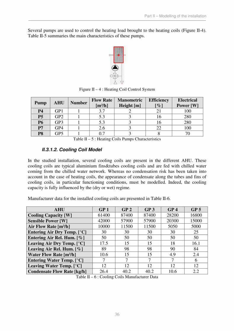
Several pumps are used to control the heating load brought to the heating coils (Figure II-4).
Table II-5 summaries the main characteristics of these pumps.
Pump AHU Number Flow Rate
[m³/h]
Manometric
Height [m]
Efficiency
[%]
Electrical
Power [W]
P4 GP1 1 3.7 2 21 100
P5 GP2 1 5.3 3 16 280
P6 GP3 1 5.3 3 16 280
P7 GP4 1 2.6 3 22 100
P8 GP5 1 0.7 3 8 70 Table II – 5 : Heating Coils Pumps Characteristics
II.3.1.2. Cooling Coil Model
In the studied installation, several cooling coils are present in the different AHU. These
cooling coils are typical aluminium fins&tubes cooling coils and are fed with chilled water
coming from the chilled water network. Whereas no condensation risk has been taken into
account in the case of heating coils, the appearance of condensate along the tubes and fins of
cooling coils, in particular functioning conditions, must be modelled. Indeed, the cooling
capacity is fully influenced by the (dry or wet) regime.
Manufacturer data for the installed cooling coils are presented in Table II-6.
AHU GP 1 GP 2 GP 3 GP 4 GP 5
Cooling Capacity [W] 61400 87400 87400 28200 16800
Sensible Power [W] 42000 57900 57900 20300 15000
Air Flow Rate [m³/h] 10000 11500 11500 5050 5000
Entering Air Dry Temp. [°C] 30 30 30 30 25
Entering Air Rel. Hum. [%] 50 50 50 50 50
Leaving Air Dry Temp. [°C] 17.5 15 15 18 16.1
Leaving Air Rel. Hum. [%] 89 98 98 90 84
Water Flow Rate [m³/h] 10.6 15 15 4.9 2.4
Entering Water Temp. [°C] 7 7 7 7 6
Leaving Water Temp. [°C] 12 12 12 12 12
Condensate Flow Rate [kg/h] 26.4 40.2 40.2 10.6 2.2 Table II – 6 : Cooling Coils Manufacturer Data
Figure II – 4 : Heating Coil Control System

Part II – Modelling of the installation
37
Complete “Mother” Model
This reference (“mother”) model threats the cooling coil as a counterflow heat exchanger by
using the model proposed by Lebrun & al. (1990), based on Merkel’s theory (F.Merkel,
1925). In this model, fully dry and fully wet regimes are described and computed
simultaneously. According to Braun’s hypothesis (Braun, J.E., Klein, S.A., Mitchell, J.W.,
1989), the regime to be considered is the one leading to the maximal cooling capacity.
According to this model, the cooling coil is finally characterized by three resistances disposed
in series : the convective resistance on the airside, the conduction resistance of the metal and
the convective resistance on the waterside.
In dry regime, the classical ε-NTU method is used to define the cooling capacity and the (dry)
effectiveness. The overall heat transfer coefficient is calculated by considering the three
thermal resistances previously quoted (equation II.3.5).
In wet regime, the air is replaced by a fictitious perfect gas, whose enthalpy is fully defined by
the actual wet bulb temperature. The corresponding cooling power and (fictitious) thermal
resistance are defined by equations (II.3.6) and (II.3.7).
(II.3.6)
(II.3.7)
(II.3.5)
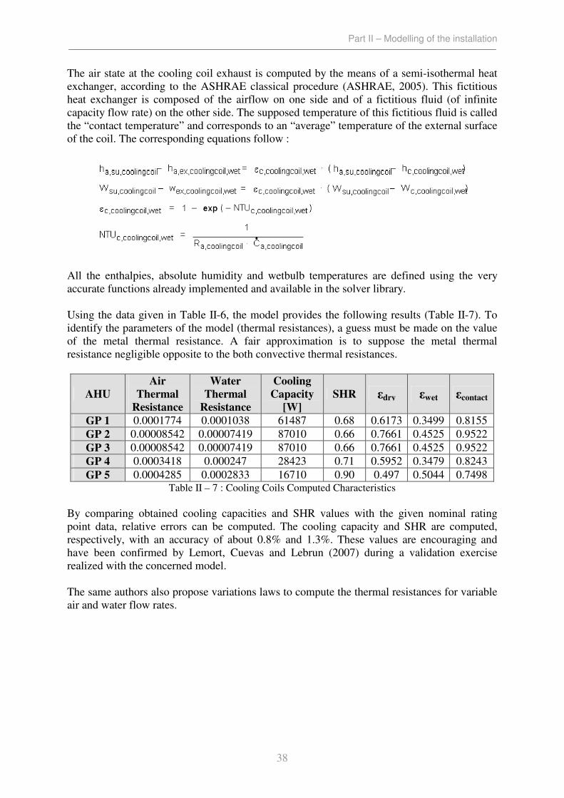
Part II – Modelling of the installation
38
The air state at the cooling coil exhaust is computed by the means of a semi-isothermal heat
exchanger, according to the ASHRAE classical procedure (ASHRAE, 2005). This fictitious
heat exchanger is composed of the airflow on one side and of a fictitious fluid (of infinite
capacity flow rate) on the other side. The supposed temperature of this fictitious fluid is called
the “contact temperature” and corresponds to an “average” temperature of the external surface
of the coil. The corresponding equations follow :
All the enthalpies, absolute humidity and wetbulb temperatures are defined using the very
accurate functions already implemented and available in the solver library.
Using the data given in Table II-6, the model provides the following results (Table II-7). To
identify the parameters of the model (thermal resistances), a guess must be made on the value
of the metal thermal resistance. A fair approximation is to suppose the metal thermal
resistance negligible opposite to the both convective thermal resistances.
AHU
Air
Thermal
Resistance
Water
Thermal
Resistance
Cooling
Capacity
[W]
SHR εdry εwet εcontact
GP 1 0.0001774 0.0001038 61487 0.68 0.6173 0.3499 0.8155
GP 2 0.00008542 0.00007419 87010 0.66 0.7661 0.4525 0.9522
GP 3 0.00008542 0.00007419 87010 0.66 0.7661 0.4525 0.9522
GP 4 0.0003418 0.000247 28423 0.71 0.5952 0.3479 0.8243
GP 5 0.0004285 0.0002833 16710 0.90 0.497 0.5044 0.7498 Table II – 7 : Cooling Coils Computed Characteristics
By comparing obtained cooling capacities and SHR values with the given nominal rating
point data, relative errors can be computed. The cooling capacity and SHR are computed,
respectively, with an accuracy of about 0.8% and 1.3%. These values are encouraging and
have been confirmed by Lemort, Cuevas and Lebrun (2007) during a validation exercise
realized with the concerned model.
The same authors also propose variations laws to compute the thermal resistances for variable
air and water flow rates.
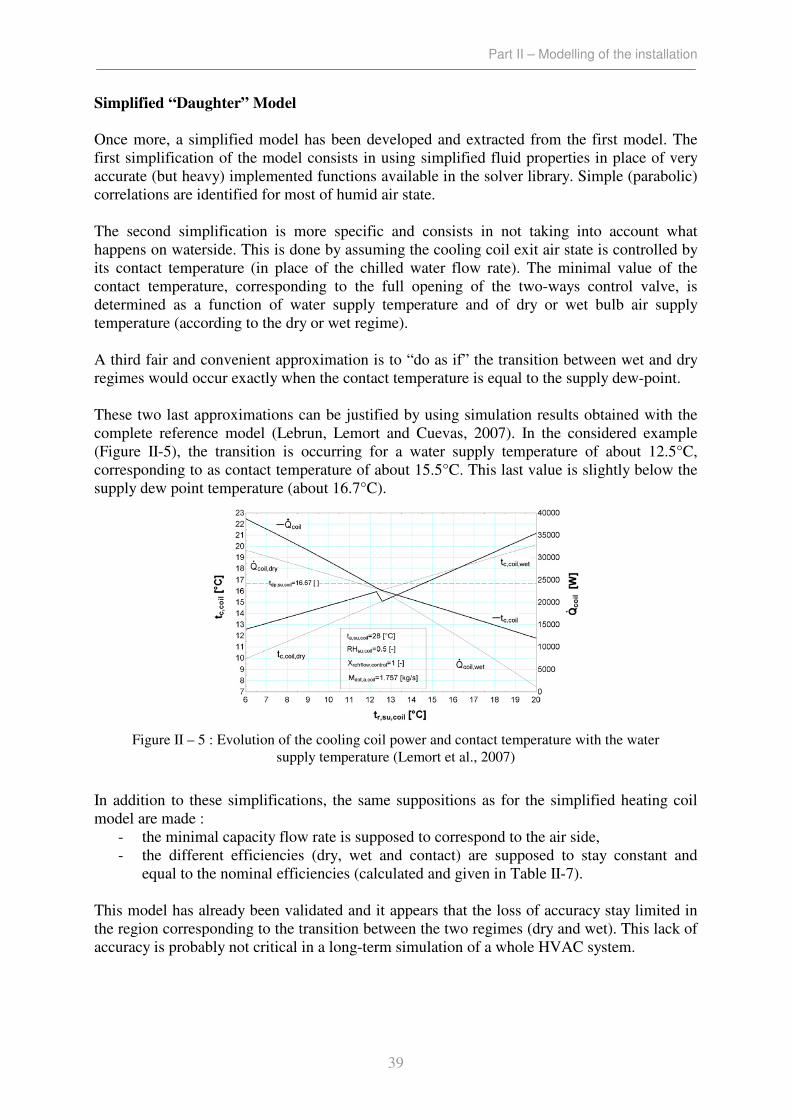
Part II – Modelling of the installation
39
Simplified “Daughter” Model
Once more, a simplified model has been developed and extracted from the first model. The
first simplification of the model consists in using simplified fluid properties in place of very
accurate (but heavy) implemented functions available in the solver library. Simple (parabolic)
correlations are identified for most of humid air state.
The second simplification is more specific and consists in not taking into account what
happens on waterside. This is done by assuming the cooling coil exit air state is controlled by
its contact temperature (in place of the chilled water flow rate). The minimal value of the
contact temperature, corresponding to the full opening of the two-ways control valve, is
determined as a function of water supply temperature and of dry or wet bulb air supply
temperature (according to the dry or wet regime).
A third fair and convenient approximation is to “do as if” the transition between wet and dry
regimes would occur exactly when the contact temperature is equal to the supply dew-point.
These two last approximations can be justified by using simulation results obtained with the
complete reference model (Lebrun, Lemort and Cuevas, 2007). In the considered example
(Figure II-5), the transition is occurring for a water supply temperature of about 12.5°C,
corresponding to as contact temperature of about 15.5°C. This last value is slightly below the
supply dew point temperature (about 16.7°C).
In addition to these simplifications, the same suppositions as for the simplified heating coil
model are made :
- the minimal capacity flow rate is supposed to correspond to the air side,
- the different efficiencies (dry, wet and contact) are supposed to stay constant and
equal to the nominal efficiencies (calculated and given in Table II-7).
This model has already been validated and it appears that the loss of accuracy stay limited in
the region corresponding to the transition between the two regimes (dry and wet). This lack of
accuracy is probably not critical in a long-term simulation of a whole HVAC system.
Figure II – 5 : Evolution of the cooling coil power and contact temperature with the water
supply temperature (Lemort et al., 2007)
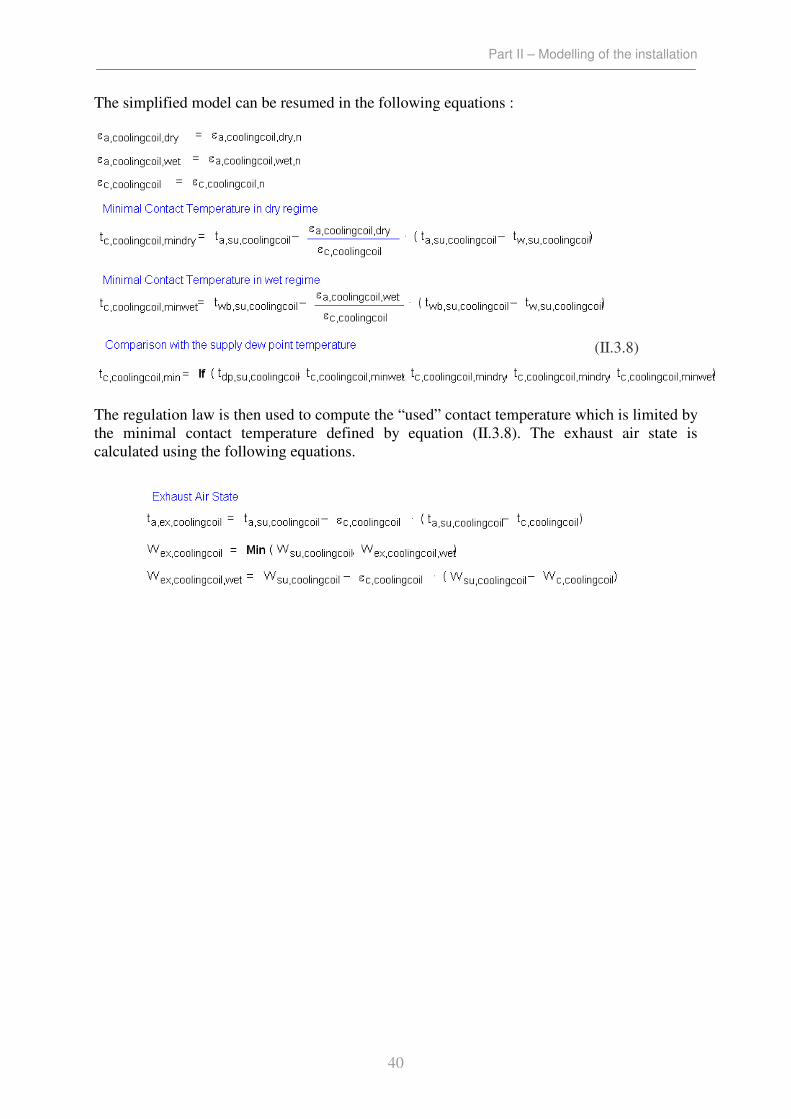
Part II – Modelling of the installation
40
The simplified model can be resumed in the following equations :
The regulation law is then used to compute the “used” contact temperature which is limited by
the minimal contact temperature defined by equation (II.3.8). The exhaust air state is
calculated using the following equations.
(II.3.8)

Part II – Modelling of the installation
41
II.3.1.3. Recovery Loop Model
Classical recovery loops include three main components : one exhaust air coil, one supply air
coil and a water (or glycol water) loop equipped with a pump (Figure II-6, left). These loops
are surely the simplest way to recover the exhaust air energy and use it to heat the fresh air
(“winter functioning mode”). According to the functioning conditions (outdoor and indoor
temperature and humidity), two regimes are possible. The heat transfer can be fully sensible
(red and blue evolutions) or partially sensible and latent (red and green evolutions) (Figure II-
6, right). In this last case, condensation occurs at the exhaust air coil. Of course, recovery
loops can be used in “summer mode” and cool the fresh air by re-heating the extracted air.
This last functioning mode is quite rare in our moderated climates.
In the present, the recovery loops are placed at the entrance of the air handling units. To avoid
the freezing risks and the related damages, recovery loops work with 25% (mass percentage)
glycol water.
Detailed “Mother” Model
The complete model is based on the principle of an air-to-air heat exchanger (Figure II-7).
The supply airside is modelled as cooling coil (working in dry or wet regime, see II.3.1.2.). Of
course the fluids are not water and air but air on the both sides. The extracted air is cooled
(primary fluid) and the fresh air is heated (secondary fluid). Knowing the nominal rating point
of the loop, this complete model is used to define the effectiveness’s (the same three
effectiveness’s as in the classical cooling coil model) of the air/air equivalent coil. The
equations will not be detailed here because of their redundant character. The results given by
this model are presented in Table II-8.
Figure II – 6 : Scheme of a Direct Recovery Loop – Typical Evolutions on Psychrometric
Diagram
Figure II – 7 : Equivalent Air to Air Heat Exchanger
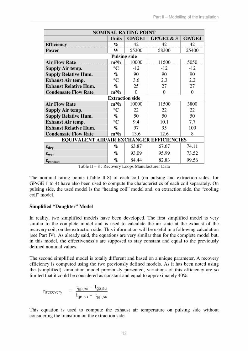
Part II – Modelling of the installation
42
NOMINAL RATING POINT
Units GP/GE1 GP/GE2 & 3 GP/GE4
Efficiency % 42 42 42
Power W 55300 58300 25400
Pulsing side
Air Flow Rate m³/h 10000 11500 5050
Supply Air temp. °C -12 -12 -12
Supply Relative Hum. % 90 90 90
Exhaust Air temp. °C 3.6 2.3 2.2
Exhaust Relative Hum. % 25 27 27
Condensate Flow Rate m³/h 0 0 0
Extraction side
Air Flow Rate m³/h 10000 11500 3800
Supply Air temp. °C 22 22 22
Supply Relative Hum. % 50 50 50
Exhaust Air temp. °C 9.4 10.1 7.7
Exhaust Relative Hum. % 97 95 100
Condensate Flow Rate m³/h 13.6 12.6 8
EQUIVALENT AIR/AIR EXCHANGER EFFICIENCIES
εdry % 63.87 67.67 74.11
εwet % 93.09 95.99 73.52
εcontact % 84.44 82.83 99.56
Table II – 8 : Recovery Loops Manufacturer Data
The nominal rating points (Table II-8) of each coil (on pulsing and extraction sides, for
GP/GE 1 to 4) have also been used to compute the characteristics of each coil separately. On
pulsing side, the used model is the “heating coil” model and, on extraction side, the “cooling
coil” model.
Simplified “Daughter” Model
In reality, two simplified models have been developed. The first simplified model is very
similar to the complete model and is used to calculate the air state at the exhaust of the
recovery coil, on the extraction side. This information will be useful in a following calculation
(see Part IV). As already said, the equations are very similar than for the complete model but,
in this model, the effectiveness’s are supposed to stay constant and equal to the previously
defined nominal values.
The second simplified model is totally different and based on a unique parameter. A recovery
efficiency is computed using the two previously defined models. As it has been noted using
the (simplified) simulation model previously presented, variations of this efficiency are so
limited that it could be considered as constant and equal to approximately 40%.
This equation is used to compute the exhaust air temperature on pulsing side without
considering the transition on the extraction side.

Part II – Modelling of the installation
43
The circulation of the glycol water in the recovery loops is ensured by several pumps. The
main characteristics of these pumps are summaries in Table II-9 .
Circuit AHU Number Flow Rate
[m³/h]
Manometric
Height [m]
Efficiency
[%]
Electrical
Power [W]
P9 GP4 1 1.6 2.5 22 50
P10 GP1 1 3.2 8 22 320
P11 GP2 1 3.2 8 22 320
P12 GP3 1 3.2 8 22 320 Table II – 9 : Recovery Loops Pumps
As already said, these recovery loops are supposed to be not regulated and to work all the year
long.

Part II – Modelling of the installation
44
II.3.1.4. Steam Humidifier Model
Only three air handlers are equipped with humidification devices (GP 2, 3 & 7). These two
first air handling units are in charge of the conditioning of the laboratories. The last air
handler (GP 7) is in charge of the “humidity-controlled room” of which the presence is not
taken into account in this analysis.
The considered steam humidifiers are able to deliver about 90kg/h of steam each. The
electrical nominal power is about 136 kWe for both (As built file, 2003).
Considering the small quantity of available information and the simplicity of theses devices,
only a simplified model will be presented and used.
Knowing the supply humidity ratio (corresponding to the humidity ratio at the cooling coil
exhaust), the exhaust desired humidity ratio (required to maintain the humidity set point in the
zone) and the air mass flow rate, it is easy to compute the steam mass flow rate (eq II.3.9).
Using an enthalpy balance to express the mixing between the air flow and the steam flow, it is
easy to calculate the air exhaust temperature (eq II.3.10).
Making supposition on water temperature at the inlet of the steam cylinder, it is possible to
compute the thermal power required to produce the wanted steam flow rate (eq II.3.11 ). A
fair supposition on the efficiency of the device enables to compute the electrical power
demand (eq II.3.12).
During simulation, the tap water temperature and the produced steam temperature are
supposed to be about, respectively, 15°C and 110°C. The efficiency of the device is supposed
to be about 95%.
This “orphan” model is not issued from a reference model but is easy to tune using
manufacturer data and several assumptions.
(II.3.9)
(II.3.10)
(II.3.11)
(II.3.12)

Part II – Modelling of the installation
45
II.3.1.5. Fan Model
Generally, air handling units are equipped with two fans, one “main fan” (pulsing side) and
one “return fan” (extraction side). Knowing the “nominal” rating points (given in as-built
documentation, Table II-10) and considering that the fans work at (“nominal”) constant air
flow rates during functioning periods (CAV system), the fan model can be resumed in a very
simple couple of equation (eq II.3.13)2.
GP1 GP2 GP3 GP4 GP5
Air Flow Rate [m³/h] 10000 11500 11500 5050 5000
Pressure Var. [Pa] 1151 1367 1367 1017 564
Efficiency [%] 78 78 78 77 74
GE1 GE2 GE3 GE4
Air Flow Rate [m³/h] 10000 11500 11500 3800
Pressure Var. [Pa] 798 1068 1068 651
Efficiency [%] 75 75 75 74
Table II – 10 : Fans Manufacturer Data
The used equations are presented below :
Equation II.3.13 is used to compute the electrical power demand of the fan. The three
remaining equations are used to calculate the air state at the exhaust of the fan (corresponding
to the entry of the distribution duct).
This “orphan” model is not issued from a reference model but is easy to tune using
manufacturer data.
II.3.1.6. Duct Model
At this moment, no duct model has been developed. Distribution duct are supposed to stay dry
(no condensation) and adiabatic (heat exchange neglected along ducts).
2 Note that the air handler GP/GE 5 (100% recirculated air mode) is equipped with a unique fan.
(II.3.13)

Part II – Modelling of the installation
46
II.3.1.7. Air Handling Unit Global Model Parameters
By adding all the components of the AHU, the global AHU model is obtained and can be
represented in the way showed in Figure II-8.
The role played and the intervention of each component is controlled by the regulation laws.
The exhaust air conditions (pulsed air conditions) can be very different according to the
functioning mode and the ambient conditions. With an aim of globalisation of the AHU
model, global parameters and characteristics are calculated using the components calculated
characteristics (efficiencies, heat transfer coefficients…etc). The characteristics of the global
AHU model are presented in Table II-11.
Units Laboratories
Global AHU model
Offices
Global AHU model
Corresponding to… GP/GE 1,2 & 3 GP/GE 4
Main fan
Flow rate m³/h 33000 5050
Pressure variation Pa 3885 1017
Efficiency % 78 77
Return fan
Flow rate m³/h 33000 3800
Pressure variation Pa 2934 651
Efficiency % 75 74
Recovery Loop
Efficiency % 40 40
Heating Coil
εheatingcoil % 38 34
Hot Water Flow rate m³/h 14.5 2.5
Cooling Coil
εcoolingcoil,dry % 73 60
εcoolingcoil,wet % 42 35
εc,coolingcoil % 90 82
Chilled Water Flow rate m³/h 40.6 4.9
Chilled Water Supply Temp. °C 7 7
Steam Humidifier
Efficiency % 90
Steam Supply Temp. °C 110
Water Supply Temp. °C 15 Table II – 11 : Parameters of the Global AHU Model
Figure II – 8 : Diagram of AHU model

Part II – Modelling of the installation
47
II.3.2. Terminal Unit Model
In this model, heating/cooling terminal units are seen as semi-isothermal heat exchangers (the
isothermal side is the indoor environment). Only one output is required : the heating/cooling
load provided by the devices. These terms intervene directly in the sensible heat gains
calculation (cf. eq. II.2.11).
In heating mode (eq II.3.14), the heating load is computed using the indoor temperature and
the supplied hot water temperature. This variable is fixed thanks to the control laws (detailed
below).
In cooling mode (eq. II.3.15), the cooling load is computed using the indoor temperature, the
constant supply chilled water temperature (corresponding to the chilled water network
temperature). The control variable X is used to modulate directly the cooling load provided to
the zone.
In the previous equations, K values correspond approximately to “heat transfer coefficients”.
These K values are determined using the given manufacturer data and supposing constant and
maximal air and water flow rates. This choice is due to the fact that terminal units control
laws are too sophisticated to be easily modelled and simulated. Further, the choice of the
maximal nominal capacity allows us to investigate many retrofit possibilities (decreasing of
the hot water temperature level for example), while knowing that technical considerations
would still be taken into account in a more detailed analysis (regulation on air and water flow
rates).Of course this approximation moves us away from reality but, the aim of this simplified
model is only the calculation of the heating and cooling loads (Figure II-9). Temperature
variations and flow rates are not taken into account here. Of course, the consumptions of the
terminal units fans are considered in the total electrical consumption.
As it has been done for the AHU model, a “globalisation work” has also been realized for the
terminal unit model. The 48 terminal units are considered as one global terminal unit, heating
or cooling the zone (offices).
This orphan model is not issued from a reference model but is easy to tune, using
manufacturer data. Indeed, only one parameter must be defined to tune this model (K value).
(II.3.14)
(II.3.15)
Figure II – 9 : Diagram of Terminal Unit Model
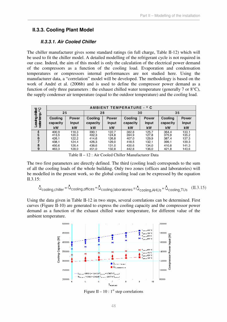
Part II – Modelling of the installation
48
II.3.3. Cooling Plant Model
II.3.3.1. Air Cooled Chiller
The chiller manufacturer gives some standard ratings (in full charge, Table II-12) which will
be used to fit the chiller model. A detailed modelling of the refrigerant cycle is not required in
our case. Indeed, the aim of this model is only the calculation of the electrical power demand
of the compressors as a function of the cooling load. Evaporation and condensation
temperatures or compressors internal performances are not studied here. Using the
manufacturer data, a “correlation” model will be developed. The methodology is based on the
work of André et al. (2006b) and is used to define the compressor power demand as a
function of only three parameters : the exhaust chilled water temperature (generally 7 or 8°C),
the supply condenser air temperature (equal to the outdoor temperature) and the cooling load.
The two first parameters are directly defined. The third (cooling load) corresponds to the sum
of all the cooling loads of the whole building. Only two zones (offices and laboratories) will
be modelled in the present work, so the global cooling load can be expressed by the equation
II.3.15:
Using the data given in Table II-12 in two steps, several correlations can be determined. First
curves (Figure II-10) are generated to express the cooling capacity and the compressor power
demand as a function of the exhaust chilled water temperature, for different value of the
ambient temperature.
(II.3.15)
Table II – 12 : Air Cooled Chiller Manufacturer Data
Figure II – 10 : 1st step correlations

Part II – Modelling of the installation
49
Basing on these curves, polynomial laws (eq II.3.16) are obtained for each series of points
(Figure II-10).
The second step is the plotting of the coefficients of the identified polynomial laws
(eq.II.3.16) as functions of the condenser supply air temperature (Figure II-11). New
polynomial laws are identified to obtain usable mathematical expressions.
The final model could be resumed in the following set of equations (eq. II.3.17)
This methodology has already been validated using a complete detailed model of air cooled
chiller. This mother model has also been validated by André & al. (2006b). Note that rating
points are re-computed with an accuracy of about 1.2%.
(II.3.16)
(II.3.17)
Figure II – 11 : 2nd
step correlations

Part II – Modelling of the installation
50
Unfortunately, these data correspond to fixed water temperature variations of 5°C on the
evaporator side and so, correspond to a variable water flow rate. In spite of this constraint the
model will be used to evaluate the performances and the electrical consumption of the chiller.
To take into account the partial-load functioning modes, a additional curve is used to convert
the full-load power already computed thank to the model previously showed. Using the
manufacturer data in part load, a curve is generated (Figure II-12). This curve plots the
Electrical Load Factor (ELF, eq II.3.19) as a function of the Cooling Load Factor (CLF, eq
II.3.18).
where evQ& is the actual cooling power demand at the evaporator, in W,
MAX,evQ& is the full-load cooling capacity in the considered conditions, in W,
cpW& is the actual electrical power demand at the compressors, in W,
MAX,cpW& is the full-load electrical power demand in the considered conditions, in W,
A polynomial law (eq II.3.20) can be extracted from this curve (Figure II-12) and can be used
in the model to establish the connection between the known CLF and the ELF which will be
used to calculate the actual compressor power demand.
(II.3.18)
(II.3.19)
Figure II – 12 : Part Load Data
(II.3.20)

Part II – Modelling of the installation
51
An additional easy calculation is realized to estimate the consumption of the condenser fans.
The consumption is supposed to be proportional to the evacuated power.
II.3.3.2. Chilled Water Network
Three pumps are used for the distribution of the chilled water (Table II-13) The first pump
(F1) fed the cooling coils of the air handling units and the second (F2), the cooling coils of the
terminal units. The third pump (PRIM) is in charge of the primary chilled water network and
ensures the water circulation in the evaporator. These pumps are not equipped with inverters,
so, we can suppose that they work in nominal conditions as soon as there is a cooling demand
in the building. Vanes ensure regulation of the chilled water network.
Circuit Number Flow Rate
[m³/h]
Manometric
Height [m]
Efficiency
[%]
Electrical
Power [W]
F1 1 49 7 56 1700
F2 1 25.4 6 42 1000
PRIM 1 70 5.5 36 3000 Table II – 13 : Chilled Water Network Pumps
II.3.4. Heating Plant Model
II.3.4.1. Condensing Boiler
Like it was the case for the chiller, the aim of the condensing boiler model is just to provide a
approximate value of the gas consumption corresponding to the energy demand of the
building. To achieve this goal, the condensing boiler is modelled by a simple constant
efficiency of about 90 % (HHV based efficiency).
II.3.4.2. Hot Water Network
Two pumps are considered in the modelling (Table II-14). The first pump (C1) fed the heating
coils of the air handling units and the second (C2), the heating coils of the terminal units. The
pumps C1 and C2 are not equipped with inverters, so, we can suppose that they work in
nominal conditions as soon as there is a heating demand in the building. Vanes ensure
regulation of these two pumps.
Circuit Number Flow Rate
[m³/h]
Manometric Height
[m]
Efficiency
[%]
Electrical
Power [W]
C1 1 16.9 2.3 22 500
C2 1 7.7 5 31 350 Table II – 14 : Hot Water Network Pumps

Part II – Modelling of the installation
52
II.4. Inputs Of The Model
In addition to the previously defined parameters (for the building and the HVAC installation),
three main types of inputs are required to perform hourly simulations : weather data,
occupancy rates and control strategies (regulation laws and set points).
II.4.1. Weather Data
To obtain usable and interesting simulation results, realistic weather data must be used as an
input of the model. In the developed model, only outdoor temperature, relative humidity (or
corresponding humidity ratio or wet bulb temperature), solar radiations on horizontal surfaces
and projection factors are applied to the building and the HVAC system. Wind contribution is
not taken into account in the concerned model.
In the present use of the model, a typical set of weather data has been used. This set of
weather data, provided in a “lookup” Table (Figure II-13), is based on averages carried out
over thirty years of measurements, realized in Uccle (Belgium). These data seems to
correspond to a “soft” year without any summer or winter peaks (as an illustration, seasonal
average dry bulb temperatures are presented in Table II-15). Some slight adaptations will be
done to test the model in more extreme conditions. Of course, if they were available, current
or more recent weather data could be used in the same way.
The given weather data is supposed to begin on 1st January, at midnight. Note that, to make
calculation easier, the hour change (occurring between summer and winter periods) is not
taken into account. The model works using “summer hours” all the year long.
Winter Spring Summer Autumn
Period 21stDec.–20
th Mar. 21
st Mar.–20
th Jun. 21
st Jun.–20
th Sept. 21
st Sept–20
th Dec.
Av. Temp.
[°C] 5.08 10.82 16.04 8.12
Table II – 15 : Typical Weather Data – Seasonal Average Outdoors Temperatures
Figure II – 13 : Weather Data (“Lookup Table”)

Part II – Modelling of the installation
53
II.4.2. Occupancy Rates
Occupancy factors are also provided in “lookup” Tables. These factors influence the
occupancy (sensible and latent) loads. In addition to these occupancy factors (appearing in
equations presented above), functioning factors are defined to take into account the starting
and the stop of the HVAC components. As already said in part I of this work, occupancy and
functioning rates are very different according to the considered zone.
II.4.2.1. Offices
Occupancy and HVAC functioning rates are plotted for a typical week in Figure II-14. From
Monday to Friday, terminal units work from 6:00 to 20:00. The AHU works also from 6:00 to
20:00. On Sunday, a re-starting is programmed using terminal units between 17:00 and 20:00.
II.4.2.2. Laboratories
Laboratories are ventilated and conditioned at maximal flow rate 24 hours per day, 7 days per
week. The occupancy varies between 6 people (during night) and 70 people between 8:00 and
17:00. Appliances function 24 hours per day too.
Figure II – 14 : Occupancy and Ventilation Rates in Offices

Part II – Modelling of the installation
54
II.4.3. Control Laws
In HVAC, control devices are very important and sophisticated. The modelling of these
equipments is quite difficult and would require to know the actual control laws.
Unfortunately, these control laws are seldom accessible for the used or the auditor. To
perform robust and accurate simulations, “home made” control laws must be built to regulate
the HVAC installation model.
To keep the calculations robust and easy to understand, only proportional control laws will be
developed.
II.4.3.1. Offices
Heating
For heating, two types of control laws have been used : “Power Control Laws” and
“Temperature Control Laws”. Initially, the model was used with “Power Control Laws”. In
this functioning mode, maximal available heating power was calculated (as a function of
different parameters) and the regulation variable (varying between 0 and 1) was used to
modulate the actual heating power. This control variable X, was calculated as a function of
the difference observed between the set point temperature and the controlled variable. The
proportionality gains used to define the control variable value are arbitrarily fixed as a
realistic compromise between control accuracy and computation stability.
“Temperature Control Laws” are based on the same principle but do not proceed on the
heating power but on the hot water temperature. Supposing that the heating devices are
working at constant flow rate (with constant efficiencies and heat transfer coefficients),
required hot water temperature is computed. This hot water temperature is obviously limited
by a maximal value, corresponding to the maximal available hot water temperature (about
80°C if hot water is produced by gas boilers). This type of regulation provides useful
information about a potential rationalization of hot water temperature levels.

Part II – Modelling of the installation
55
The heating of the zone is mainly ensured by the terminal units and the “closed-loop AHU’
(GP5, considered as a large terminal unit). The AHU (GP/GE4) is supposed to function as a
“air treatment” device. So, terminal units ensure the follow-up of the set point (ta,in,heatingTU,set is
about 23°C) and the AHU’s heating coil intervene only to bring the fresh pulsed air at a given
temperature (ta,pulsion,set is about 18°C for example). Control laws are presented below (eq.
II.4.1).
Cooling
As it has been said during the description of the cooling coil model, this component is
controlled using the contact temperature. The minimal available contact temperature is
computed and used to define the actual required contact temperature, as a function of the
control variable (eq. II.4.2). The principle is the same as for heating mode, cooling is mainly
ensured by terminal units (ta,in,coolingTU,set is about 24°C); AHU cooling coil intervene in “back
up” if indoor temperature pass over a given temperature (ta,in,heatingGP,set = 25°C for example).
Terminal units cooling coils are controlled using a “Power Control Law”.
(II.4.2)
(II.4.1)

Part II – Modelling of the installation
56
II.4.3.2. Laboratories
The situation is a bit different in the laboratories. Indeed, air conditioning is fully ensured by
the three AHU (GP/GE 1 to 3). Control laws are similar to the AHU control strategies
presented for the offices. Lower and higher temperature limits are, respectively, 22.5 and 23.5
°C. Humidity is regulated using the same type of control laws.
II.5. Outputs Of The Model
The outputs expected are mainly :
- the indoor air conditions, hour by hour and the variations of these conditions
compared to the defined temperature and humidity set points,
- the heating, cooling, electrical power demands and energy consumptions for each
component of the installation, hour by hour, all along the simulation period,
- the power and primary energy consumptions (gas and electricity) for each component
and for the whole installation (per zone or not), hour by hour, all along the simulation
period,
- information about actual performances of the different components (efficiencies,
COP) and about the way they are used (flow rates, temperatures,…etc).
In addition to these outputs (corresponding to the actual installation), retrofit opportunities
will be modelled and simulated on a similar year. These results will be used to realize a
economical comparison between the different solutions.

Part III – Simulation Results & Analysis
57
PART III : SIMULATION RESULTS AND ANALYSIS

Part III – Simulation Results & Analysis
58
III.1. Introduction
The aim of this part is to present the first simulation results. At the moment, only the present
installation (described in the first part of this work) is considered. These results have already
been presented in the frame of the IEA Annex48 project (Lebrun, J., Bertagnolio, S., 2007a
and 2007b).
III.2. Present Situation – Simulation Results
A first simulation of the two considered zones (offices and laboratories) is made, using the
previously defined model. As it has been said in the second part of this work, as-built data
have been used to define the parameters and inputs of the model. This first run is supposed to
estimate the thermal behaviour of the two zones during a “typical” year. Only a few results
will be presented here. More interesting results will be presented and detailed during the
analysis and the study of retrofit possibilities (Part IV).
III.2.1. Temperature Profiles
The temperature profiles of the both zone are quite different and vary as a function of the
occupancy loads, set points, ventilation rates and solar exposures.
III.2.1.1. Laboratories
Figure III-1 shows the indoor-outdoor January temperature profile for the zone III
(laboratories). This month has been chosen because of its low average temperature and its
cold peak (outdoor temperature reaching –10°C).
Figure III – 1 : January Temperature Profile - Laboratories

Part III – Simulation Results & Analysis
59
The red curve shows the asked hot water temperature, used to heat the fresh air passing trough
the AHU heating coils. In spite of the high air flow rate and the low outdoor temperature (at
time ~ 200h), the asked temperature does not exceed 60°C. This fact can be explained by the
high internal sensible loads (occupancy, appliances and lights) decreasing the heating demand
of the zone. Even with this “low” hot water temperature, the indoor set point (23°C) is well,
but not perfectly, maintained. Indeed, the indoor temperature curve is quite horizontal and
near to 22°C but is not exactly equal to the winter set-point (23°C) because of the used of
proportional control laws. A dynamic (PI) control would permit a more efficient respect of the
set point and could need a higher hot water temperature. The pulsed air temperature (blue
curve) is rather near to the indoor temperature and generally varies between 20 and 26°C.
The relative humidity set point is also well maintained and near to the set point value (50%).
The remaining off-set is still due to the limitations of proportional control laws.
Figure III-2 shows the August temperature profile. Because of the 24/24 ventilation, heating
and cooling demands follow each other. Generally, heating and cooling demands appear
during night and day respectively. Of course, during this summer month (characterized by an
average temperature of about 17°C), hot water asked temperature is lower. The pulsed air
temperature is now lower and can reach 19°C. The indoor temperature floats between 23 and
25°C and the summer set-point (24°C) is quite well maintained in spite of the remaining off-
set. These quite high temperatures have been observed during several visits of the building.
The relative humidity is quite well maintained during “dry” hours (hours requiring
humidification) but reaches 60 and 70% during “wet” hours (hours requiring de-
humidification). This high relative humidity values are due to the fact that de-humidification
is not controlled in the building and intervenes only if the fresh air cooling reaches a given
level. This quite high relative humidity has been observed in reality.
Figure III – 2 : August Temperature Profile - Laboratories

Part III – Simulation Results & Analysis
60
A “thermal comfort” index has been computed and takes into account the variations of more
than 2°C compared to the set point (23°C). For the whole year, no “cold hour” (characterized
by an indoor temperature lower than 21°C) has been counted and only 9 “hot hours”
(characterized by an indoor temperature higher than 26°C) have been counted. These quite
good results confirm the fact that simple proportional control laws are able to ensure a good
following of the set points. The same “thermal comfort” indices will be used to quantify the
quality of the set-points follow-up.
III.2.1.2. Offices
The same temperature profile has been generated for the offices. Considering the variable
occupancy rate, daily and weekly variations are easily observable. Considering that two
heating devices (AHU heating coil and terminal units heating coils) ensure the heating of the
zone, two hot water temperature curves are plotted on Figure III-3. The red one corresponds
to the terminal units heating coils and the blue one, to the AHU heating coil. Because of the
variable occupancy (and functioning) rate(s), the indoor temperature decreases a lot during
unoccupied (and non-conditioned) periods. This fact is due to the low thermal capacity of the
zone (light walls, large open plan floor with no important thermal mass). These important
variations cause important heating demands (and so, important hot water temperature levels),
on very short periods, at the re-starting of the installation (each day at 6:00 and on Sunday).
The rest of the time (majority of time), the asked hot water temperature stay quite limited and
varies between 30 and 50°C. This time, the heating water asked temperature reaches the
maximal hot water temperature (85°C). However, the temperature set-point is well maintained
during occupied periods and the control strategy seems to be efficient, even if it causes high
peaks of heating demand.
Figure III – 3 : January Temperature Profile - Offices
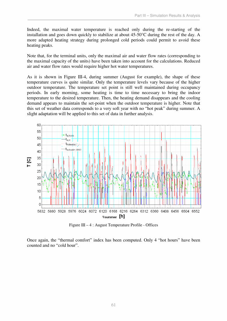
Part III – Simulation Results & Analysis
61
Indeed, the maximal water temperature is reached only during the re-starting of the
installation and goes down quickly to stabilize at about 45-50°C during the rest of the day. A
more adapted heating strategy during prolonged cold periods could permit to avoid these
heating peaks.
Note that, for the terminal units, only the maximal air and water flow rates (corresponding to
the maximal capacity of the units) have been taken into account for the calculations. Reduced
air and water flow rates would require higher hot water temperatures.
As it is shown in Figure III-4, during summer (August for example), the shape of these
temperature curves is quite similar. Only the temperature levels vary because of the higher
outdoor temperature. The temperature set point is still well maintained during occupancy
periods. In early morning, some heating is time to time necessary to bring the indoor
temperature to the desired temperature. Then, the heating demand disappears and the cooling
demand appears to maintain the set-point when the outdoor temperature is higher. Note that
this set of weather data corresponds to a very soft year with no “hot peak” during summer. A
slight adaptation will be applied to this set of data in further analysis.
Once again, the “thermal comfort” index has been computed. Only 4 “hot hours” have been
counted and no “cold hour”.
Figure III – 4 : August Temperature Profile - Offices
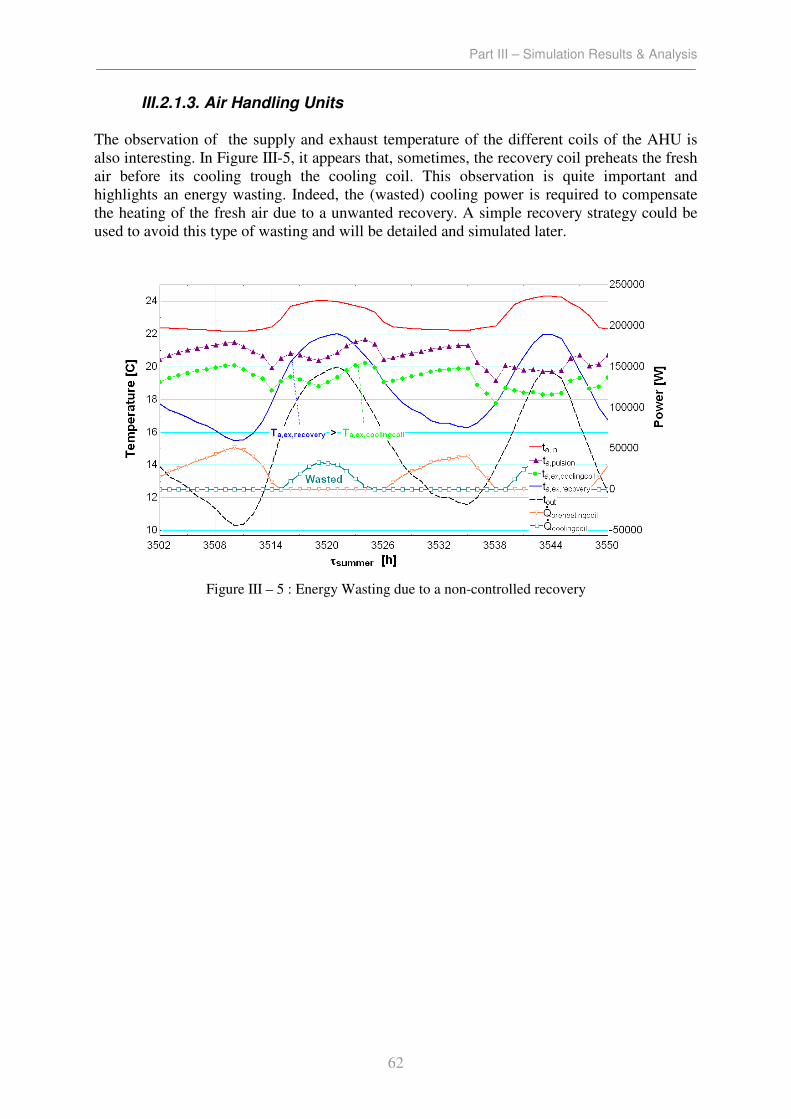
Part III – Simulation Results & Analysis
62
III.2.1.3. Air Handling Units
The observation of the supply and exhaust temperature of the different coils of the AHU is
also interesting. In Figure III-5, it appears that, sometimes, the recovery coil preheats the fresh
air before its cooling trough the cooling coil. This observation is quite important and
highlights an energy wasting. Indeed, the (wasted) cooling power is required to compensate
the heating of the fresh air due to a unwanted recovery. A simple recovery strategy could be
used to avoid this type of wasting and will be detailed and simulated later.
Figure III – 5 : Energy Wasting due to a non-controlled recovery
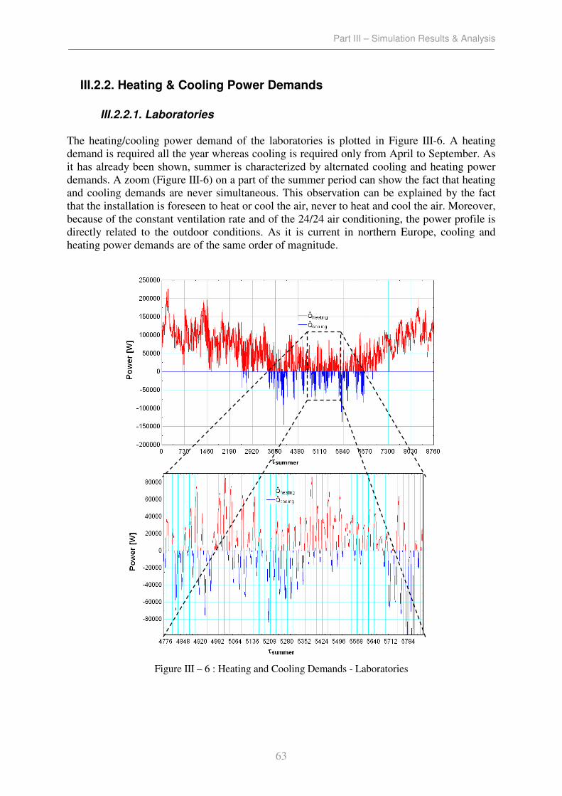
Part III – Simulation Results & Analysis
63
III.2.2. Heating & Cooling Power Demands
III.2.2.1. Laboratories
The heating/cooling power demand of the laboratories is plotted in Figure III-6. A heating
demand is required all the year whereas cooling is required only from April to September. As
it has already been shown, summer is characterized by alternated cooling and heating power
demands. A zoom (Figure III-6) on a part of the summer period can show the fact that heating
and cooling demands are never simultaneous. This observation can be explained by the fact
that the installation is foreseen to heat or cool the air, never to heat and cool the air. Moreover,
because of the constant ventilation rate and of the 24/24 air conditioning, the power profile is
directly related to the outdoor conditions. As it is current in northern Europe, cooling and
heating power demands are of the same order of magnitude.
Figure III – 6 : Heating and Cooling Demands - Laboratories
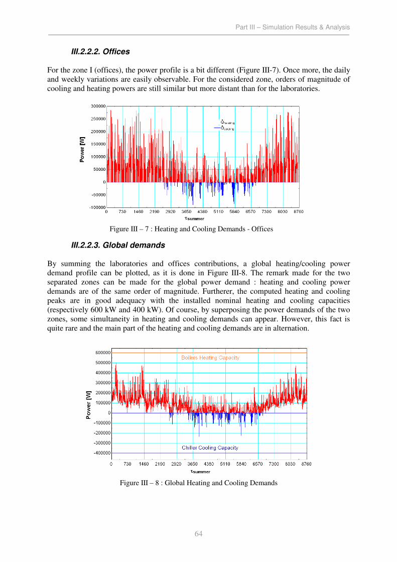
Part III – Simulation Results & Analysis
64
III.2.2.2. Offices
For the zone I (offices), the power profile is a bit different (Figure III-7). Once more, the daily
and weekly variations are easily observable. For the considered zone, orders of magnitude of
cooling and heating powers are still similar but more distant than for the laboratories.
III.2.2.3. Global demands
By summing the laboratories and offices contributions, a global heating/cooling power
demand profile can be plotted, as it is done in Figure III-8. The remark made for the two
separated zones can be made for the global power demand : heating and cooling power
demands are of the same order of magnitude. Furtherer, the computed heating and cooling
peaks are in good adequacy with the installed nominal heating and cooling capacities
(respectively 600 kW and 400 kW). Of course, by superposing the power demands of the two
zones, some simultaneity in heating and cooling demands can appear. However, this fact is
quite rare and the main part of the heating and cooling demands are in alternation.
Figure III – 7 : Heating and Cooling Demands - Offices
Figure III – 8 : Global Heating and Cooling Demands
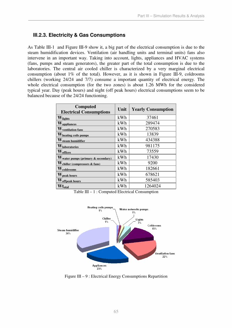
Part III – Simulation Results & Analysis
65
III.2.3. Electricity & Gas Consumptions
As Table III-1 and Figure III-9 show it, a big part of the electrical consumption is due to the
steam humidification devices. Ventilation (air handling units and terminal units) fans also
intervene in an important way. Taking into account, lights, appliances and HVAC systems
(fans, pumps and steam generators), the greater part of the total consumption is due to the
laboratories. The central air cooled chiller is characterized by a very marginal electrical
consumption (about 1% of the total). However, as it is shown in Figure III-9, coldrooms
chillers (working 24/24 and 7/7) consume a important quantity of electrical energy. The
whole electrical consumption (for the two zones) is about 1.26 MWh for the considered
typical year. Day (peak hours) and night (off peak hours) electrical consumptions seem to be
balanced because of the 24/24 functioning.
Computed
Electrical Consumptions Unit Yearly Consumption
Wlights kWh 37461
Wappliances kWh 289474
Wventilation fans kWh 270583
Wheating coils pumps kWh 13839
Wsteam humidifier kWh 434388
Wlaboratories kWh 981175
Woffices kWh 73559
Wwater pumps (primary & secondary) kWh 17430
Wchiller (compressors & fans) kWh 9200
Wcoldrooms kWh 182661
Wpeak hours kWh 678621
Woffpeak hours kWh 585403
Wtotal kWh 1264024
Table III – 1 : Computed Electrical Consumption
Figure III – 9 : Electrical Energy Consumptions Repartition
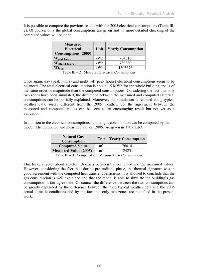
Part III – Simulation Results & Analysis
66
It is possible to compare the previous results with the 2005 electrical consumptions (Table III-
2). Of course, only the global consumptions are given and no more detailed checking of the
computed values will be done.
Measured
Electrical
Consumptions (2005)
Unit Yearly Consumption
Wpeak hours kWh 764316
Woffpeak hours kWh 739360
Wtotal kWh 1503676 Table III – 2 : Measured Electrical Consumptions
Once again, day (peak hours) and night (off peak hours) electrical consumptions seem to be
balanced. The total electrical consumption is about 1.5 MWh for the whole building and is of
the same order of magnitude than the computed consumptions. Considering the fact that only
two zones have been simulated, the difference between the measured and computed electrical
consumptions can be partially explained. Moreover, the simulation is realized using typical
weather data, surely different from the 2005 weather. So, the agreement between the
measured and computed values can be seen as an encouraging result but not yet as a
validation.
In addition to the electrical consumptions, natural gas consumption can be computed by the
model. The computed and measured values (2005) are given in Table III-3.
Natural Gas
Consumption Unit Yearly Consumption
Computed Value m³ 76814
Measured Value (2005) m³ 124231 Table III – 3 : Computed and Measured Gas Consumptions
This time, a factor about a factor 1.6 exists between the computed and the measured values.
However, considering the fact that, during pre-auditing phase, the thermal signature was in
good agreement with the computed heat transfer coefficients, it is allowed to conclude that the
gas consumption is well explained and that the model is able to simulate the building’s gas
consumption in fair agreement. Of course, the difference between the two consumptions can
be greatly explained by the difference between the used typical weather data and the 2005
actual climatic conditions and by the fact that only two zones are modelled in the present
work.

Part III – Simulation Results & Analysis
67
III.3. Conclusions
The presented results seem in quite good adequacy with the reality. However, because of the
model limitations and of the assumptions, the results have to be considered as qualitative
better than as quantitative information. The numeric values are obtained using simplified
models and artificial typical weather data and are more a slightly fuzzy reflection than a
photograph of the reality. But the computed numeric values of gas and electricity
consumptions have been, quite successfully, compared to the 2005 actual consumptions.
Considering the different contributions into the global electrical consumption, the main effort
must be done on the steam humidifiers. Moreover, a specific study would have to be made on
to rationalize the consumptions of fans and appliances. The comfort and working
requirements (fresh air rate, humidity and temperature set points) would have to be studied
and, if possible, rationalized. For example, in laboratories, the rate of fresh air could be
decreased during non-working time (night). The reason of using expensive steam
humidification instead of full new water adiabatic humidification (for example) could be
discussed too. These adaptations and improvements, valid in most cases, are not the aim of
this work and are left in care of the company’s management.
More specific conclusions can be made and will be useful in the following :
- The water supply temperatures asked by the AHUs heating coils are quite low (for the
considered set of weather data); they do not exceed 60°C,
- The water supply temperatures asked by the TU heating coils stay limited during
prolonged heating periods (30-50°C), but reach high levels during re-starting of the
installation.
- Inside a same zone, heating and cooling demands are never simultaneous,
- Among the two zones considered, heating and cooling demands are sometimes
simultaneous, but such superposition stay quite rare and limited in amplitude.
Electrical consumptions and performances of the installation will be more detailed later and
compared to the simulation results obtained during the study of the retrofit possibilities.

Part IV – Retrofit & Improvement Opportunities
68
PART IV : RETROFIT & IMPROVEMENT OPPORTUNITIES

Part IV – Retrofit & Improvement Opportunities
69
IV.1. Plant Modification
IV.1.1. Recovery Strategy
Nowadays, the recovery loops are functioning at maximal glycol water flow rate when the
ventilation is switched on. Even if the building (or the zone) is not in heating demand,
recovery loops ensure the heat exchange between the supply and exhaust air flows. During
cold periods, the recovery loops ensure the pre-heating of the air with a quite good efficiency.
During very hot periods (the outdoor temperature is higher than the indoor temperature), the
recovery loops can be used to cool partially the fresh air. During average temperature periods
(between 18 and 21°C for example), recovery loops can heat the fresh air (to 21-22°C) before
its cooling in the cooling coil (to be pulsed at 18-19°C). The idea of a recovery strategy is to
stop the circulation of the glycol water in the loops to avoid a pre-heating of the air if a
cooling is required. So, the cooling demand would decrease and an economy could be made
on the chiller consumption. The simpler strategy is to stop the recovery between 18 and 26°C
(outdoor temperature).
IV.1.2. Reversible Heat Pumping
Generally, two heat pumping modes are envisaged (IEA Annex48) :
- the condenser heat recovery (simultaneous cooling and heating demands),
- the reversible heat pumping (non-simultaneous cooling and heating demands).
In spite of this distinction, the principle is unique : a water/water chiller (also called heat
pump) can be connected on its evaporator and condenser sides to, the chilled water and hot
water networks, respectively.
In the case of condenser heat recovery, the evaporator is connected to a cooling demand (and,
if necessary, to an additional heat source). At the same time, the condenser of the chiller/heat
pump is connected to a heating demand (and, if necessary, to an additional cooling device, as
cooling tower) and covers (partially or totally) the heating demand.
In the case of reversible heat pumping, cooling and heating demands are rarely simultaneous.
So, the two functioning modes of the machine (chiller and heat pump) are distinct and not
simultaneous. This strategy requires more powerful heat source (on evaporator side) and heat
sink (on condenser side). Indeed, in chiller mode, the condenser rejected heat is not used and
must be evacuated, for example, with the help of a (direct or indirect contact) cooling tower.
In heat pump mode, the evaporator must be connected to a reliable heat source.
As previously explained, the building considered is characterized by comparable
(simultaneous or not) heating and cooling demands, according to the period of the year. The
winter is mainly characterized by its heating demand. During this season, the cooling demand
is almost or completely null. During summer, the building heating and cooling demands are
alternated according to the day/night cycle. However, cooling and heating demands could be
sometimes simultaneous in different rooms or parts of the building.
So, in the present case, according to the period of the year and to simultaneity of the heating
and cooling demands, both reversible heat pumping and condenser heat recovery strategies
could be used to satisfy the building cooling and heating demands.
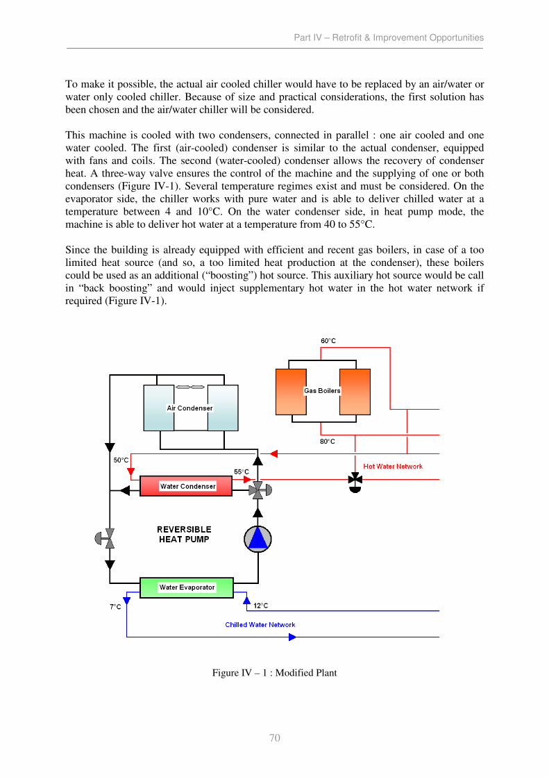
Part IV – Retrofit & Improvement Opportunities
70
To make it possible, the actual air cooled chiller would have to be replaced by an air/water or
water only cooled chiller. Because of size and practical considerations, the first solution has
been chosen and the air/water chiller will be considered.
This machine is cooled with two condensers, connected in parallel : one air cooled and one
water cooled. The first (air-cooled) condenser is similar to the actual condenser, equipped
with fans and coils. The second (water-cooled) condenser allows the recovery of condenser
heat. A three-way valve ensures the control of the machine and the supplying of one or both
condensers (Figure IV-1). Several temperature regimes exist and must be considered. On the
evaporator side, the chiller works with pure water and is able to deliver chilled water at a
temperature between 4 and 10°C. On the water condenser side, in heat pump mode, the
machine is able to deliver hot water at a temperature from 40 to 55°C.
Since the building is already equipped with efficient and recent gas boilers, in case of a too
limited heat source (and so, a too limited heat production at the condenser), these boilers
could be used as an additional (“boosting”) hot source. This auxiliary hot source would be call
in “back boosting” and would inject supplementary hot water in the hot water network if
required (Figure IV-1).
Figure IV – 1 : Modified Plant

Part IV – Retrofit & Improvement Opportunities
71
Whenever the heating of the zones considered can be ensured by hot water at 55°C or less, the
boilers could be used in condensing (high efficiency) mode. In some cases, hot water at 75-
80°C could be required and the boilers would work in non-condensing mode. Note that the
boilers stay also installed to satisfy the heating demands of the other zones and floors of the
building.
On the heat source side, the available heat must be recovered using additional water/air coils.
These auxiliary heat transfer surfaces must be installed in the extraction duct, downstream of
the recovery coils already installed. To recover the largest part of the heat available, the heat
pump is supposed to be able to work if necessary at the regime 9/4°C (entering and leaving
evaporator water temperatures).
The indoor air is extracted at conditions 23°C/50% (laboratories set-points) and at a global
flow rate of 33000m³/h. Downstream of the direct recovery coil, the air temperature varies
between 12°C (cold day with direct recovery in heating mode) and 26°C (hot day with direct
recovery in cooling mode). The additional air/water coils will be designed to allow an optimal
heat recovery to supply the heat pump evaporator. Practical considerations, as available space
in extraction ducts and pumping consumption, will be taken into account and discussed later.
IV.1.3. Change Over Technique & Re-starting
Heating the building with hot water at 55°C could be problematic. Indeed, the actual heat
exchangers (AHU and TU heating coils) are designed to be supplied with hot water at 75-
80°C. The lowering of water supply temperature from 75-80°C to 55°C could make problems
in the follow-up of the set-points. Two adaptations will be made to ensure the satisfaction of
the demands : the use of a change over technique and the programming of new re-starting
strategies.
The laboratories are only heated by the air handling units GP1,2 & 3. Additional heating
surfaces must be found to ensure the heating of the zone. Hopefully, heating and cooling
demands are never simultaneous in a same zone. So, during heating periods, the cooling coil
constitutes a un-used heat transfer surface. The idea of the change over technique is to use this
available heat transfer surface to post-heat the air. For a given air handler and for a parallel
supplying of the two coils the change over technique is illustrated in Figure IV-2. The
possibility of series supplying (to increase the counter-flow effect) has also to be considered.
The change over technique has another advantage and would allow, by using an extended heat
transfer surface, a decreasing of the hot water temperature, and so, an increasing of the heat
pump performances.
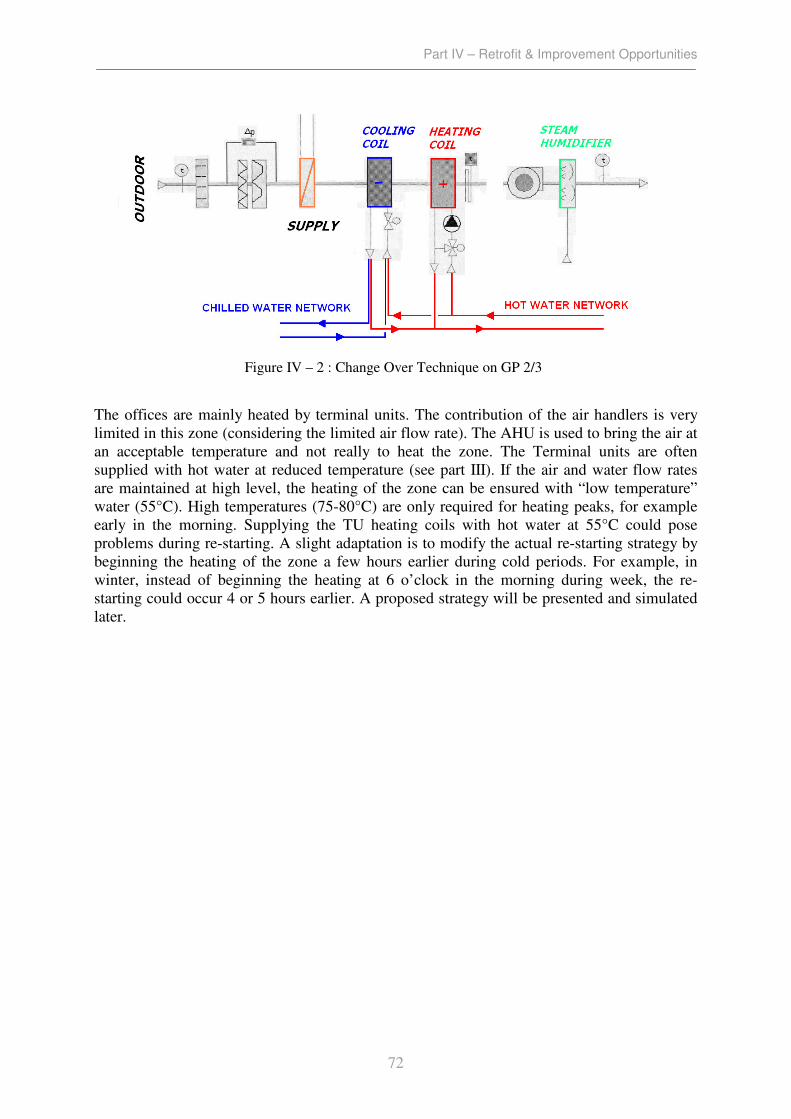
Part IV – Retrofit & Improvement Opportunities
72
The offices are mainly heated by terminal units. The contribution of the air handlers is very
limited in this zone (considering the limited air flow rate). The AHU is used to bring the air at
an acceptable temperature and not really to heat the zone. The Terminal units are often
supplied with hot water at reduced temperature (see part III). If the air and water flow rates
are maintained at high level, the heating of the zone can be ensured with “low temperature”
water (55°C). High temperatures (75-80°C) are only required for heating peaks, for example
early in the morning. Supplying the TU heating coils with hot water at 55°C could pose
problems during re-starting. A slight adaptation is to modify the actual re-starting strategy by
beginning the heating of the zone a few hours earlier during cold periods. For example, in
winter, instead of beginning the heating at 6 o’clock in the morning during week, the re-
starting could occur 4 or 5 hours earlier. A proposed strategy will be presented and simulated
later.
Figure IV – 2 : Change Over Technique on GP 2/3

Part IV – Retrofit & Improvement Opportunities
73
IV.1.4. Thermal Energy Storage
The idea of a thermal energy storage appears during the analysis of the heating and cooling
power demands (see Part III). The alternations between these two demands hide a real
potential for thermal energy storage. Indeed, supposing that, during summer, the heat
production is totally ensured by the heat pump (what will be probably the case), the produced
cool at the heat pump evaporator could be stored and used during the following cooling
demand period. So , the use of cool storage allows heat recovery chillers to meet night time
heating loads directly, while storing chilled water to meet the next day’s cooling load (Dorgan
et al., 1999; Roth et al., 2006)
A brief (static) example is detailed in Figure IV-3. between 22:00 and 10:00, the heat
production (about 610kWh) is ensured by the heat pump. At the same time, on the evaporator
side, the produced cold energy (about 457.5 kWh, supposing a COP of about 4 for the heat
pump) is stored in a storage tank of about 80m³ (corresponding to 465 kWh, for a pure water
storage with a ∆T of 5°C). From 10:00 until the drain of the storage, the cooling demand is
ensured by the stored cold energy. This part of the cooling demand is totally free ! The
production of the remaining cooling demand (372.5 kWh) is ensured by the chiller.
Even if the heating demand is not sufficient to satisfy the following cooling demand,
considering the electricity costs, it is more interesting to produce the cold energy by night. In
fact, the use of this storage allows to move the chiller consumption from day to night. This
technique is called the “load shifting”.
In addition to these two advantages, a thermal energy storage system is able to takes
advantage of lower outdoor temperatures (allowing better performances of the air condenser).
Moreover, the TES system can be used to increase the number of hours that chiller operates at
high efficiency by controlling the TES discharge rate to coincide with the chiller’s most
efficient operational regime. This energy impact varies with the part-load characteristics of
the chiller (Roth et al., 2006).
Figure IV – 3 : Cool Thermal Energy Storage Use
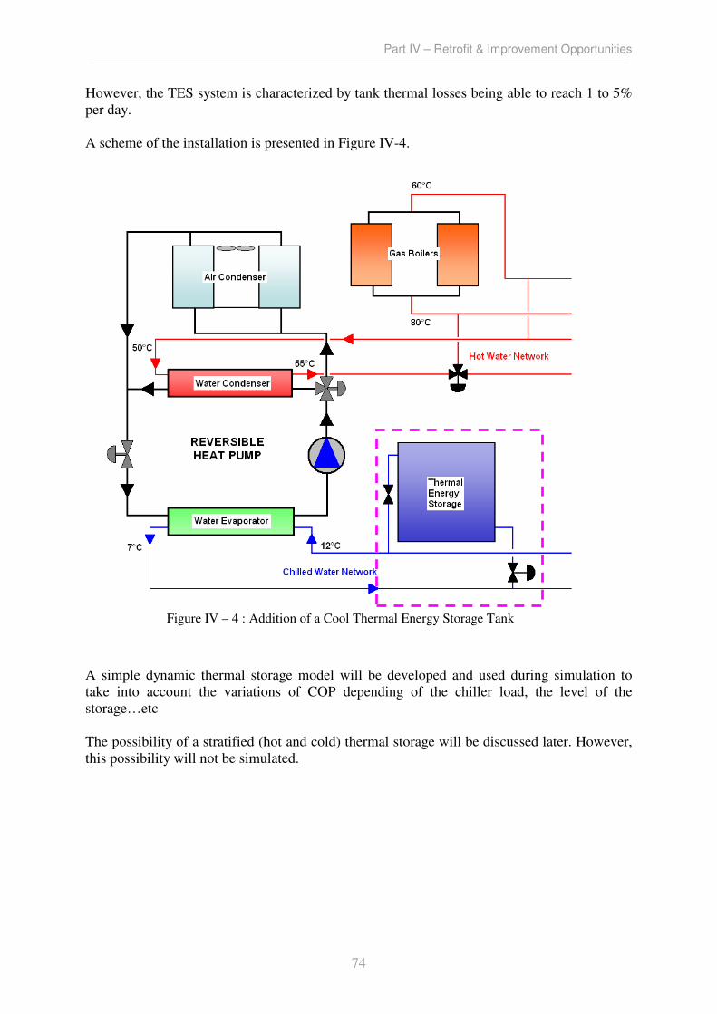
Part IV – Retrofit & Improvement Opportunities
74
However, the TES system is characterized by tank thermal losses being able to reach 1 to 5%
per day.
A scheme of the installation is presented in Figure IV-4.
A simple dynamic thermal storage model will be developed and used during simulation to
take into account the variations of COP depending of the chiller load, the level of the
storage…etc
The possibility of a stratified (hot and cold) thermal storage will be discussed later. However,
this possibility will not be simulated.
Figure IV – 4 : Addition of a Cool Thermal Energy Storage Tank
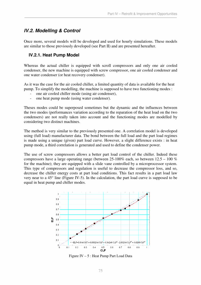
Part IV – Retrofit & Improvement Opportunities
75
IV.2. Modelling & Control
Once more, several models will be developed and used for hourly simulations. These models
are similar to those previously developed (see Part II) and are presented hereafter.
IV.2.1. Heat Pump Model
Whereas the actual chiller is equipped with scroll compressors and only one air cooled
condenser, the new machine is equipped with screw compressor, one air cooled condenser and
one water condenser (or heat recovery condenser).
As it was the case for the air cooled chiller, a limited quantity of data is available for the heat
pump. To simplify the modelling, the machine is supposed to have two functioning modes :
- one air cooled chiller mode (using air condenser),
- one heat pump mode (using water condenser).
Theses modes could be superposed sometimes but the dynamic and the influences between
the two modes (performances variation according to the reparation of the heat load on the two
condensers) are not really taken into account and the functioning modes are modelled by
considering two distinct machines.
The method is very similar to the previously presented one. A correlation model is developed
using (full load) manufacturer data. The bond between the full load and the part load regimes
is made using a unique (given) part load curve. However, a slight difference exists : in heat
pump mode, a third correlation is generated and used to define the condenser power.
The use of screw compressors allows a better part load control of the chiller. Indeed these
compressors have a large operating range (between 25-100% each, so between 12.5 – 100 %
for the machine); they are equipped with a slide vane controlled by a microprocessor system.
This type of compressors and regulation is useful to decrease the compressor loss, and so,
decrease the chiller energy costs at part load conditions. This fact results in a part load law
very near to a 45° line (Figure IV-5). In the calculation, the part load curve is supposed to be
equal in heat pump and chiller modes.
Figure IV – 5 : Heat Pump Part Load Data

Part IV – Retrofit & Improvement Opportunities
76
IV.2.2. Heat Source Model
The aim of the is model is not the accurate calculation of the recovered heat at the heat source
of the heat pump but only the estimation of the available (or recoverable) power by installing
an additional water/air coil in the extraction duct and by connecting it to the heat pump
evaporator (Figure IV-6).
Of course, the heat source available power will not always be totally used but is only
computed to know the limitations of the heat source and the rate of intervention of the boilers
(as back boosting heating devices).
First, using the recovery loop model presented in the second part of this work, the extracted
air state (temperature and humidity) is computed at the exhaust of the recovery coil. This
calculation is made on GP/GE 1,2 & 3.
Then, heating source available is computed using the extraction air state at the exhaust of the
static recovery loops as an input and using a classical cooling coil model. Of course, the
needed heat transfer surface would have to be designed and optimised. For more easiness, the
additional recovery coils are supposed to be the as the existing ones. This choice is justified
because by the dimensions of the duct. The efficiencies of these coils are used to compute the
maximal recoverable power. These coils are supplied with chilled water coming from the heat
pump evaporator at 4°C (minimal evaporator exhaust temperature). The choice of this
temperature is arbitrary but justified to calculate the maximal power recoverable. The water
flow rate is also fixed at a value corresponding approximately to a temperature variation of
5°C on the water side.
The over cost due to pumping and ventilation (additional head loss) will be estimated later.
Note that, to protect this new coil from freezing, the use of glycol water instead of pure water
could be required. To avoid the overcost caused by the transformation of the current chilled
(pure) water network by a chiller glycol water network, a plate heat exchanger could be
designed and installed between the chilled water network and the glycol loop circulating in
Figure IV – 6 : Heat Source Scheme
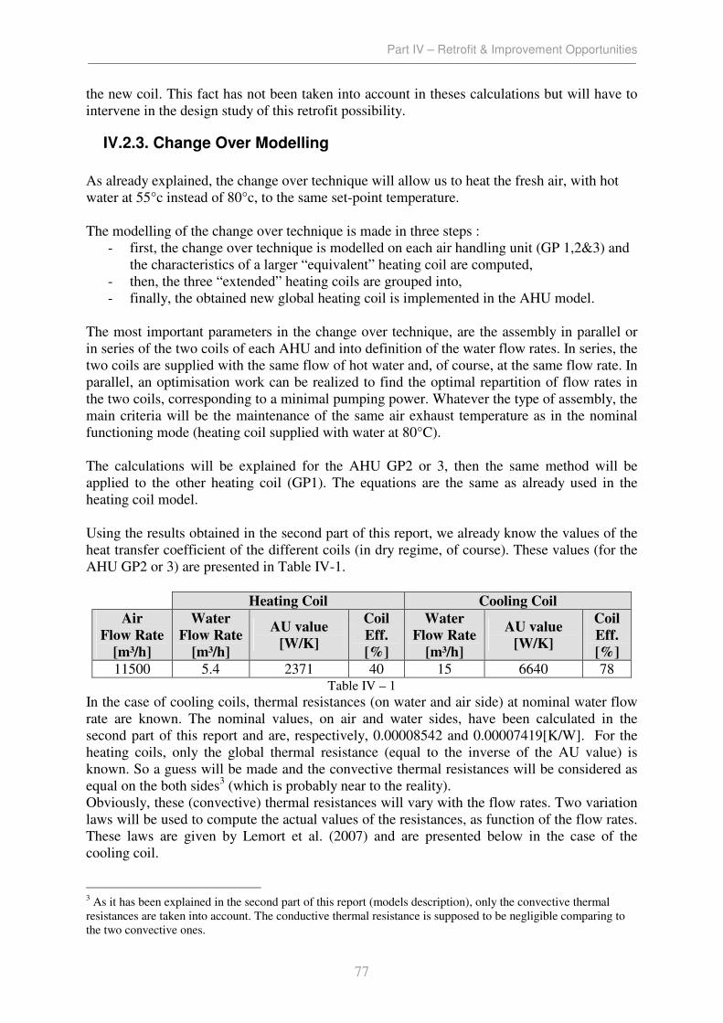
Part IV – Retrofit & Improvement Opportunities
77
the new coil. This fact has not been taken into account in theses calculations but will have to
intervene in the design study of this retrofit possibility.
IV.2.3. Change Over Modelling
As already explained, the change over technique will allow us to heat the fresh air, with hot
water at 55°c instead of 80°c, to the same set-point temperature.
The modelling of the change over technique is made in three steps :
- first, the change over technique is modelled on each air handling unit (GP 1,2&3) and
the characteristics of a larger “equivalent” heating coil are computed,
- then, the three “extended” heating coils are grouped into,
- finally, the obtained new global heating coil is implemented in the AHU model.
The most important parameters in the change over technique, are the assembly in parallel or
in series of the two coils of each AHU and into definition of the water flow rates. In series, the
two coils are supplied with the same flow of hot water and, of course, at the same flow rate. In
parallel, an optimisation work can be realized to find the optimal repartition of flow rates in
the two coils, corresponding to a minimal pumping power. Whatever the type of assembly, the
main criteria will be the maintenance of the same air exhaust temperature as in the nominal
functioning mode (heating coil supplied with water at 80°C).
The calculations will be explained for the AHU GP2 or 3, then the same method will be
applied to the other heating coil (GP1). The equations are the same as already used in the
heating coil model.
Using the results obtained in the second part of this report, we already know the values of the
heat transfer coefficient of the different coils (in dry regime, of course). These values (for the
AHU GP2 or 3) are presented in Table IV-1.
Heating Coil Cooling Coil
Air
Flow Rate
[m³/h]
Water
Flow Rate
[m³/h]
AU value
[W/K]
Coil
Eff.
[%]
Water
Flow Rate
[m³/h]
AU value
[W/K]
Coil
Eff.
[%]
11500 5.4 2371 40 15 6640 78 Table IV – 1
In the case of cooling coils, thermal resistances (on water and air side) at nominal water flow
rate are known. The nominal values, on air and water sides, have been calculated in the
second part of this report and are, respectively, 0.00008542 and 0.00007419[K/W]. For the
heating coils, only the global thermal resistance (equal to the inverse of the AU value) is
known. So a guess will be made and the convective thermal resistances will be considered as
equal on the both sides3 (which is probably near to the reality).
Obviously, these (convective) thermal resistances will vary with the flow rates. Two variation
laws will be used to compute the actual values of the resistances, as function of the flow rates.
These laws are given by Lemort et al. (2007) and are presented below in the case of the
cooling coil.
3 As it has been explained in the second part of this report (models description), only the convective thermal
resistances are taken into account. The conductive thermal resistance is supposed to be negligible comparing to
the two convective ones.

Part IV – Retrofit & Improvement Opportunities
78
Considering that only the water flow rate will vary, the first equation won’t be used in the
calculations.
IV.2.3.1. Parallel Assembly
The situation is a bit different in this second assembly. The two coils are supplied with hot
water coming directly from the hot water network. This time, the idea is to optimise the flow
rates repartition in the two coils to minimize the “pumping cost”. Of course, the constrain of
the exhaust air temperature stay the main design criteria.
Figure IV-7 shows the principle of the calculations and the main results.
Imposing the exhaust air temperature, and using the water flow rate in the heating coil as the
parameter, the model gives the required cooling coil water flow rate. The values presented in
Figure IV-7 correspond to the optimal values.
As already said, the optimum has been computed to minimize the pumping consumption.
Considering a pump efficiency of 20%, the results are presented in Figure IV-8. Electrical
pump powers are plotted as function of the flow rates ratio (flow rate in heating coil / flow
Figure IV – 7 : Change Over – Parallel Assembly Model

Part IV – Retrofit & Improvement Opportunities
79
rate in cooling coil). The both flow rate can vary between 0 and the nominal value of the coil
(5.4m³/h for the heating coil and 15m³/h for the cooling coil).
The optimum (minimal total pumping power) point (green point) is plotted on Figure IV-8
and corresponds to a flow rate ratio of about 95% (the water flow rate is a bit more important
in the cooling coil than in the heating coil). The corresponding pumping power is about 9W.
However, in spite of this lower pumping power, the total flow rate coming from the hot water
network is greater than before. The nominal water flow rate (5.4m³/h) is now multiplied by a
factor 1.2 (total water flow rate = 3.129 + 3.287 = 6.416 m³/h).
Of course, this optimisation exercise is presented as an illustration and would have to be
completed by a more global study of the head loss in the water networks.
IV.2.3.2. Series Assembly
In this mode, the counter-flow effect is maximized by supplying the two coils in series. First,
the heating coil is supplied with hot water coming from the hot water network. Then, the
cooling coil is supplied with the hot water coming from the heating coil. Of course, the hot
water flow rate is the same in the two coils.
The calculation principle is presented in Figure IV-9. Supply and exhaust air conditions and
flow rate are known and imposed by the heating coil nominal values. Knowing the supply hot
water temperature, the water flow rate (4.026 m³/h) is computed to obtain the wanted exhaust
air temperature (33.9°C).
Figure IV – 8 : Pumping Cost Minimization
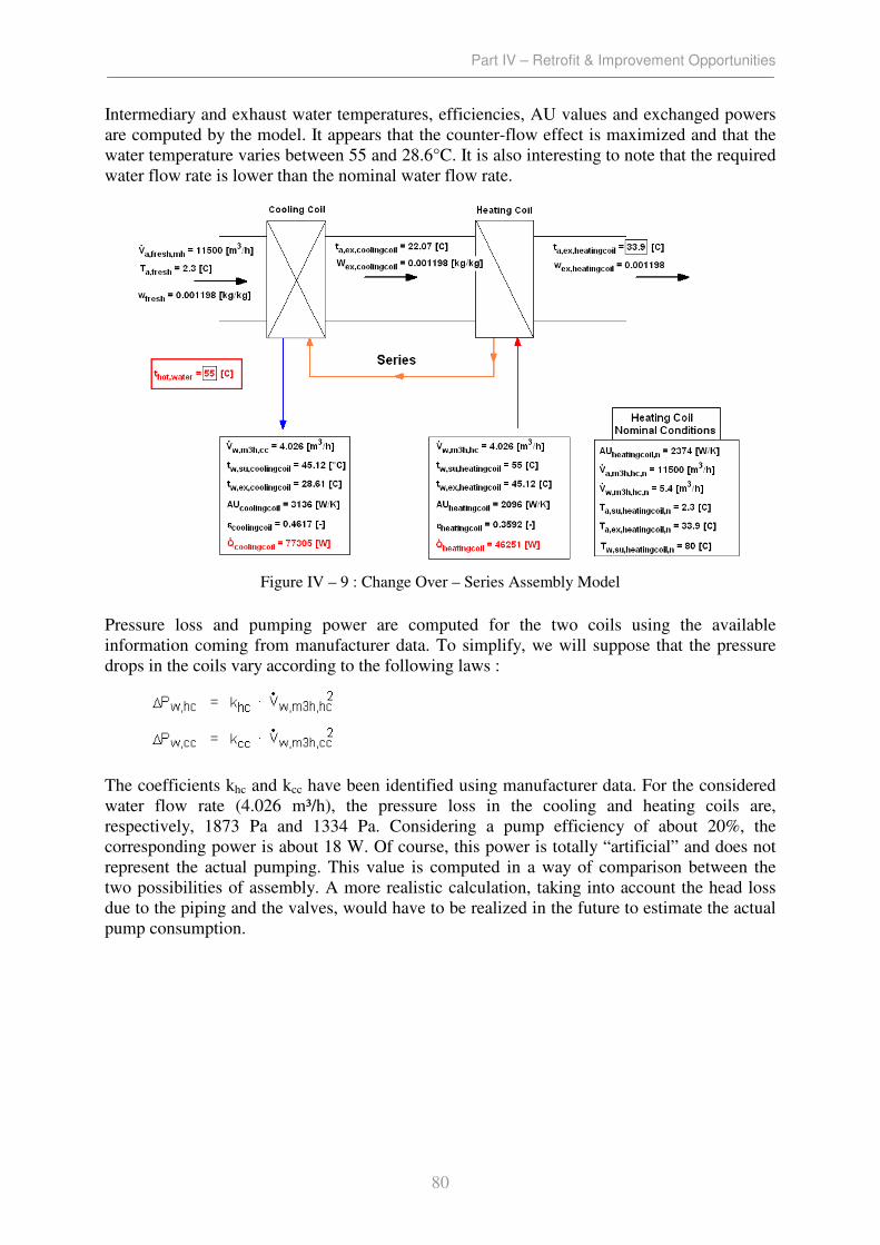
Part IV – Retrofit & Improvement Opportunities
80
Intermediary and exhaust water temperatures, efficiencies, AU values and exchanged powers
are computed by the model. It appears that the counter-flow effect is maximized and that the
water temperature varies between 55 and 28.6°C. It is also interesting to note that the required
water flow rate is lower than the nominal water flow rate.
Pressure loss and pumping power are computed for the two coils using the available
information coming from manufacturer data. To simplify, we will suppose that the pressure
drops in the coils vary according to the following laws :
The coefficients khc and kcc have been identified using manufacturer data. For the considered
water flow rate (4.026 m³/h), the pressure loss in the cooling and heating coils are,
respectively, 1873 Pa and 1334 Pa. Considering a pump efficiency of about 20%, the
corresponding power is about 18 W. Of course, this power is totally “artificial” and does not
represent the actual pumping. This value is computed in a way of comparison between the
two possibilities of assembly. A more realistic calculation, taking into account the head loss
due to the piping and the valves, would have to be realized in the future to estimate the actual
pump consumption.
Figure IV – 9 : Change Over – Series Assembly Model
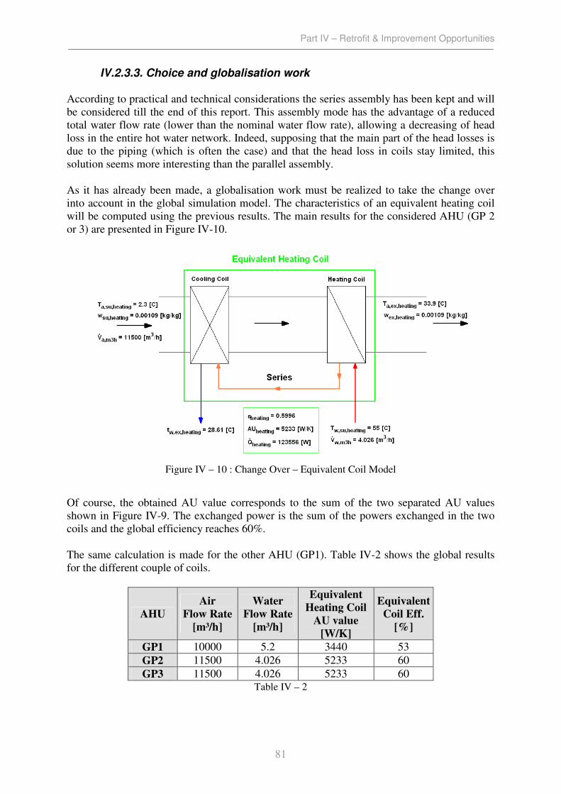
Part IV – Retrofit & Improvement Opportunities
81
IV.2.3.3. Choice and globalisation work
According to practical and technical considerations the series assembly has been kept and will
be considered till the end of this report. This assembly mode has the advantage of a reduced
total water flow rate (lower than the nominal water flow rate), allowing a decreasing of head
loss in the entire hot water network. Indeed, supposing that the main part of the head losses is
due to the piping (which is often the case) and that the head loss in coils stay limited, this
solution seems more interesting than the parallel assembly.
As it has already been made, a globalisation work must be realized to take the change over
into account in the global simulation model. The characteristics of an equivalent heating coil
will be computed using the previous results. The main results for the considered AHU (GP 2
or 3) are presented in Figure IV-10.
Of course, the obtained AU value corresponds to the sum of the two separated AU values
shown in Figure IV-9. The exchanged power is the sum of the powers exchanged in the two
coils and the global efficiency reaches 60%.
The same calculation is made for the other AHU (GP1). Table IV-2 shows the global results
for the different couple of coils.
AHU
Air
Flow Rate
[m³/h]
Water
Flow Rate
[m³/h]
Equivalent
Heating Coil
AU value
[W/K]
Equivalent
Coil Eff.
[%]
GP1 10000 5.2 3440 53
GP2 11500 4.026 5233 60
GP3 11500 4.026 5233 60 Table IV – 2
Figure IV – 10 : Change Over – Equivalent Coil Model

Part IV – Retrofit & Improvement Opportunities
82
Then the second step consists to use these values to define the characteristics (Table IV-3) of
a global heating coil (implemented in the global Air Handling Unit model).
Global Air
Flow Rate
[m³/h]
Global Water
Flow Rate
[m³/h]
Global Heating Coil
AU value
[W/K]
Global Eff.
[%]
33000 13.252 13906 58 Table IV – 3
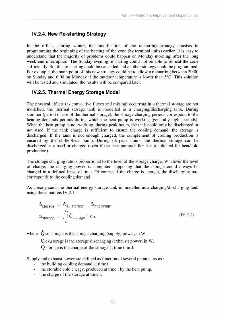
Part IV – Retrofit & Improvement Opportunities
83
IV.2.4. New Re-starting Strategy
In the offices, during winter, the modification of the re-starting strategy consists in
programming the beginning of the heating of the zone (by terminal units) earlier. It is easy to
understand that the majority of problems could happen on Monday morning, after the long
week-end interruption. The Sunday evening re-starting could not be able to re-heat the zone
sufficiently. So, this re-starting could be cancelled and another strategy could be programmed.
For example, the main point of this new strategy could be to allow a re-starting between 20:00
on Sunday and 6:00 on Monday if the outdoor temperature is lower than 5°C. This solution
will be tested and simulated, the results will be compared later.
IV.2.5. Thermal Energy Storage Model
The physical effects (as convective fluxes and mixing) occurring in a thermal storage are not
modelled, the thermal storage tank is modelled as a charging/discharging tank. During
summer (period of use of the thermal storage), the storage charging periods correspond to the
heating demands periods during which the heat pump is working (generally night periods).
When the heat pump is not working, during peak hours, the tank could only be discharged or
not used. If the tank charge is sufficient to ensure the cooling demand, the storage is
discharged. If the tank is not enough charged, the complement of cooling production is
ensured by the chiller/heat pump. During off-peak hours, the thermal storage can be
discharged, not used or charged (even if the heat pump/chiller is not solicited for heat/cold
production).
The storage charging rate is proportional to the level of the storage charge. Whatever the level
of charge, the charging power is computed supposing that the storage could always be
charged in a defined lapse of time. Of course, if the charge is enough, the discharging rate
corresponds to the cooling demand.
As already said, the thermal energy storage tank is modelled as a charging/discharging tank
using the equations IV.2.1.
where Q& su,storage is the storage charging (supply) power, in W,
Q& ex,storage is the storage discharging (exhaust) power, in W,
Q storage is the charge of the storage at time t, in J,
Supply and exhaust power are defined as function of several parameters as :
- the building cooling demand at time t,
- the storable cold energy, produced at time t by the heat pump,
- the charge of the storage at time t.
(IV.2.1)
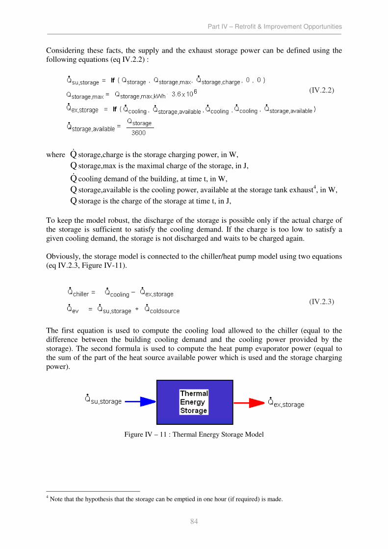
Part IV – Retrofit & Improvement Opportunities
84
Considering these facts, the supply and the exhaust storage power can be defined using the
following equations (eq IV.2.2) :
where Q& storage,charge is the storage charging power, in W,
Q storage,max is the maximal charge of the storage, in J,
Q& cooling demand of the building, at time t, in W,
Q storage,available is the cooling power, available at the storage tank exhaust4, in W,
Q storage is the charge of the storage at time t, in J,
To keep the model robust, the discharge of the storage is possible only if the actual charge of
the storage is sufficient to satisfy the cooling demand. If the charge is too low to satisfy a
given cooling demand, the storage is not discharged and waits to be charged again.
Obviously, the storage model is connected to the chiller/heat pump model using two equations
(eq IV.2.3, Figure IV-11).
The first equation is used to compute the cooling load allowed to the chiller (equal to the
difference between the building cooling demand and the cooling power provided by the
storage). The second formula is used to compute the heat pump evaporator power (equal to
the sum of the part of the heat source available power which is used and the storage charging
power).
4 Note that the hypothesis that the storage can be emptied in one hour (if required) is made.
(IV.2.2)
(IV.2.3)
Figure IV – 11 : Thermal Energy Storage Model

Part IV – Retrofit & Improvement Opportunities
85
IV.2.6. Control Strategy
First, each hour, the functioning of the installation can be classified in one of these two
categories :
- If there is NO heating demand, the possible cooling production is ensured by the cool
thermal storage or by the chiller. In this case, the chiller works as a air cooled chiller
and the water condenser is not used.
- If there is heating demand, the possible simultaneous cooling demand is added to the
heat pump evaporator cold power. This time, the heat is sent to the hot water network
trough the water condenser but can also be partially evacuated trough the air cooled
condenser.
For this second category, a control strategy has been imagined. It is presented hereafter in the
shape of an algorithm and has been also implemented on EES.
The variables used are :
- Q& ev,available = maximal available power on evaporator side (heat source power,
possible cooling demand power and possible storage charging power).
- Q& cd,available = maximal available power on condenser side, function of
Q& ev,available and of temperatures.
- Q& ev,min = minimal cooling power which have to be produced on the evaporator side
(possible cooling demand power and storage charging power) < Q& ev,available
- Q& cd,min = corresponding heating power on the condenser side
- Q& heating = heating demand of the two zones
- Q& boiler = heating power produced by the boilers (working in “back boosting” mode)
- Q& cd,HP = the actual hot power produced at the water condenser
- Q& ev,HP = corresponding cooling power produced at the evaporator
- Q& used,heatsource = part of the heat source power which has been used to produce the
asked heating power.

Part IV – Retrofit & Improvement Opportunities
86
Control Strategy :
IF Q& cd,available < Q& heating
Q& boiler = Q& heating - Q& cd,available
Q& cd,HP = Q& cd,available
Q& ev,HP = Q& ev,available
In this first case, the heating demand could not be fully satisfied by the heat pump (the heat
source on evaporator side is too limited). The boilers work in “back boosting”.
ELSE IF Q& cd,available > Q& heating
Q& boiler = 0
Q& cd,HP = Q& heating
In this second case, the heat pump is able to satisfy the whole heating demand but two
possibilities must still be envisaged.
IF Q& cd,min < Q& heating
Q& AirCondenser = 0
Q& ev,HP = Q& ev,min + Q& used,heatsource
In this first “sub-case”, the minimal cooling power to produce on the evaporator side does not
cause a sufficient heating load on water condenser side to satisfy the heating demand. The
heat source (extracted air) is partially used. The exact heating demand is produced on water
condenser side. The air condenser does not work.
ELSE IF Q& cd,min > Q& heating
Q& AirCondenser = Q& cd,min - Q& heating
Q& ev,HP =Q& ev,min
Q& used,heatsource = 0
In this last “sub-case”, the minimal cooling power to produce on evaporator side cause the
production of a too important heating load on condenser side. The water condenser ensures
the providing of the heating power to the hot water network. The remaining heat is evacuated
trough the air cooled condenser. This sub-case occurs generally when low heating demands
occur simultaneously with important cooling demand.
END
END
This control strategy is supposed to be near to reality and will be used to calculate the
consumptions of the new installation.

Part V – Modified Plant – Simulation Results
87
PART V : MODIFIED PLANT - SIMULATION RESULTS

Part V – Modified Plant – Simulation Results
88
V.1. Introduction
Using the models described in the fourth part of this report, some simulations are made to
compare the different retrofit possibilities. Five installations (called systems n°1,2,3,4 and 5)
are to be considered :
1) Actual Installation : Heating by gas boilers, Cooling by Air-cooled chiller, no recovery
strategy,
2) Addition of a simple recovery strategy : the brine circulation in recovery loops is
stopped for an outdoor temperature between 18 and 26°C,
3) Replacement of the Air-cooled chiller by a dual-condenser chiller and heating by
using it in heat pump mode with the extracted air as heat source,
4) Use of a change over technique in AHUs and programming of an adapted re-starting
strategy,
5) Addition of a cool thermal energy storage to allow “load shifting”.
The first case has already been presented in the third part of this report. The simulation results
for the others cases will be detailed and presented hereafter. To allow comparison, the
simulations have been realized using the same set of weather data.
A second (fictitious) set of weather data (Figure V-1) has been generated and used for some
additional simulations. This weather data set has been obtained by superposing the original
temperature curve and a sinusoid (black curve). The relative humidity and solar radiations are
not modified.
This superposition gives a more severe annual temperature profile, characterized by a colder
winter and a hotter summer.
Figure V - 1 : Temperature Data Modification

Part V – Modified Plant – Simulation Results
89
V.2. Simulation Results
V.2.1. System n°1 – Actual Installation
The simulation results (based on original weather data set) obtained thanks to the modelling
of the actual installation (building and HVAC system) have been presented in the third part of
this report. They are now more detailed in Table V-1.
Table V - 1
The conversions of the heating and cooling demands in gas and electrical consumptions are
realized using the boiler and chiller models, respectively.
The cooling demand (Qcooling demand) is the cooling power consumed by the cooling coils of the
HVAC installation (AHU and TU). The low value of this demand is due to the used weather
data set and its “soft” summer. The corresponding chiller electrical consumption is also quite
low and give a yearly global COP (Coefficient of Performances : cooling energy demand/
electrical compressors consumption) of about 5. By taking into account the auxiliary
consumptions (as primary pumps and condenser fans), the EER (Energy Efficiency Ratio :
cooling energy demand/ [electrical compressors, condenser fans and evaporator pumps
consumptions]) can be computed and is about 3.1. These values might be a bit optimistic. The
used model could be improved by using more accurate and complete part load data.
5 Primary Hot water network pumps (C1,C2,C3 & C4)
6 Primary Cold water network pumps (F1 & F2)
7 sum of 2 & 3
8 Evaporator Pumps (PRIM)
Electrical
Consumptions Unit Yearly Consumption
Wlights kWh 37461
Wappliances kWh 289474
Wventilation fans kWh 270583
Wheating coils pumps kWh 13839
Wsteam humidifier kWh 434388
Whot water network pumps5 kWh 8311
Wcold water network pumps6 kWh 4350
Wwater networks pumps (secondary)7 kWh 12661
Wchiller (compressors only) kWh 8592
Wcondenser fans kWh 608
Wevaporator pump (primary)8 kWh 4769
Qcooling demand kWh 43082
Wcoldrooms kWh 182661
Wpeak hours kWh 678621
Woffpeak hours kWh 585403
Wtotal kWh 1264024
Computed
Consumption Unit Yearly Consumption
Qheating demand kWh 765862
Qgas kWh 850958
Vgas m³ 76814
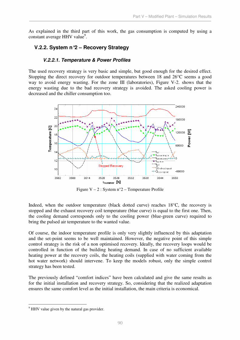
Part V – Modified Plant – Simulation Results
90
As explained in the third part of this work, the gas consumption is computed by using a
constant average HHV value9.
V.2.2. System n°2 – Recovery Strategy
V.2.2.1. Temperature & Power Profiles
The used recovery strategy is very basic and simple, but good enough for the desired effect.
Stopping the direct recovery for outdoor temperatures between 18 and 26°C seems a good
way to avoid energy wasting. For the zone III (laboratories), Figure V-2. shows that the
energy wasting due to the bad recovery strategy is avoided. The asked cooling power is
decreased and the chiller consumption too.
Indeed, when the outdoor temperature (black dotted curve) reaches 18°C, the recovery is
stopped and the exhaust recovery coil temperature (blue curve) is equal to the first one. Then,
the cooling demand corresponds only to the cooling power (blue-green curve) required to
bring the pulsed air temperature to the wanted value.
Of course, the indoor temperature profile is only very slightly influenced by this adaptation
and the set-point seems to be well maintained. However, the negative point of this simple
control strategy is the risk of a non optimised recovery. Ideally, the recovery loops would be
controlled in function of the building heating demand. In case of no sufficient available
heating power at the recovery coils, the heating coils (supplied with water coming from the
hot water network) should intervene. To keep the models robust, only the simple control
strategy has been tested.
The previously defined “comfort indices” have been calculated and give the same results as
for the initial installation and recovery strategy. So, considering that the realized adaptation
ensures the same comfort level as the initial installation, the main criteria is economical.
9 HHV value given by the natural gas provider.
Figure V – 2 : System n°2 – Temperature Profile

Part V – Modified Plant – Simulation Results
91
Figure V-3 shows the difference between the two cooling demand profiles. The first
(n°1,black curve) corresponds to the initial situation whereas the second (n°2, blue curve)
corresponds to the new recovery strategy. The absolute difference is plotted in red and vary
between 0 and 25kW.
Figure V – 3 : System n°2 - Cooling Demand Profiles

Part V – Modified Plant – Simulation Results
92
V.2.2.2. Economical Aspect & Conclusion
To quantify the influence of this slight adaptation on the performances of the installation, the
detailed consumptions are shown in Table V-2.
Table V - 2
As it has been said, the simple and arbitrary characters of the new recovery strategy could
cause an increasing of the gas consumption in addition to the decreasing of the electrical
consumption (because of the removal of the energy wasting). Unfortunately, this fact has not
been avoided and the gas consumptions increases slightly.
The variations of the electrical and gas consumptions are presented in Table V-3.
Unit System n°1 System n°2
Qcooling demand kWh 43082 30788
Wchiller kWh 13969 11229
Wtotal kWh 1264024 1258382
Elec. Cost € 119125 118578
Vgas m³ 76814 77249
Gas Cost € 33051 33238 Table V - 3
Electrical
Consumptions Unit Yearly Consumption
Wlights kWh 37461
Wappliances kWh 289474
Wventilation fans kWh 270583
Wheating coils pumps kWh 13056
Wsteam humidifier kWh 432497
Wlaboratories kWh 978529
Woffices kWh 73531
Whot water network pumps kWh 8485
Wcold water network pumps kWh 3948
Wwater networks pumps (secondary) kWh 12433
Wchiller (compressors only) kWh 6463
Wcondenser fans kWh 438
Wevaporator pump (primary) kWh 4328
Qcooling demand kWh 30788
Wcoldrooms kWh 182661
Wpeak hours kWh 675258
Woffpeak hours kWh 583124
Wtotal kWh 1258382
Heat Consumption Unit Yearly Consumption
Qheating demand kWh 770197
Qgas kWh 855774
Vgas m³ 77249

Part V – Modified Plant – Simulation Results
93
The chiller electrical consumption (compressors, fans and evaporator pumps) decreases of
about 2719 kWh. The decreasing of the total electrical consumption is a bit greater due to the
variation of the distribution pumps consumption (function of the cooling/heating coils
functioning rate). The global saving is of about 547€ / year (for the considered typical year)10
.
The gas consumption increases from 76784 m³ to 77224m³. This increasing is due to the
simplicity of the control strategy and corresponds to an overcost of about 187€ / year. So, the
net saving is of about 360€ / year. The investment is supposed to be null because, no more
equipments have to be installed. In fact, the cost is limited to the definition of an additional
control law in the BEM (Building & Energy Management) software. Even if this
improvement seems quite marginal and has reduced consequences, it must be taken into
account, because of its simplicity and because the aim of this work is the improvement of the
global performances of the installation.
This improvement seems to be successful and is kept for the following simulations. These
numerical results will be considered as reference for the future comparisons.
10
Electricity costs are computed by using actual and recent tariffs. The prices are : 0.1155 €/kWh,peak and
0.0696 €/kWh,offpeak. The gas tariff (HHV) is 0.0348€/kWhgas.
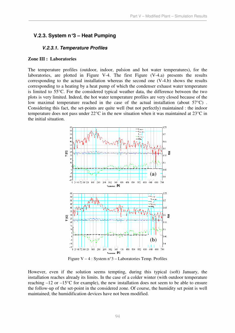
Part V – Modified Plant – Simulation Results
94
V.2.3. System n°3 – Heat Pumping
V.2.3.1. Temperature Profiles
Zone III : Laboratories
The temperature profiles (outdoor, indoor, pulsion and hot water temperatures), for the
laboratories, are plotted in Figure V-4. The first Figure (V-4.a) presents the results
corresponding to the actual installation whereas the second one (V-4.b) shows the results
corresponding to a heating by a heat pump of which the condenser exhaust water temperature
is limited to 55°C. For the considered typical weather data, the difference between the two
plots is very limited. Indeed, the hot water temperature profiles are very closed because of the
low maximal temperature reached in the case of the actual installation (about 57°C) .
Considering this fact, the set-points are quite well (but not perfectly) maintained : the indoor
temperature does not pass under 22°C in the new situation when it was maintained at 23°C in
the initial situation.
However, even if the solution seems tempting, during this typical (soft) January, the
installation reaches already its limits. In the case of a colder winter (with outdoor temperature
reaching –12 or –15°C for example), the new installation does not seem to be able to ensure
the follow-up of the set-point in the considered zone. Of course, the humidity set point is well
maintained; the humidification devices have not been modified.
(a)
(b)
Figure V – 4 : System n°3 – Laboratories Temp. Profiles

Part V – Modified Plant – Simulation Results
95
To illustrate this fact, the previously presented modified weather data set is used. The results
for the both systems (n°1 and n°3) are shown in Figure V-5 (a and b, respectively).
This time, the difference is marked and obvious. In the initial situation, the hot water
temperature reaches 60°C to maintain the set point. Obviously, in the new situation the hot
water temperature is limited to 55°C. So, the follow-up of the set-point is not guaranteed and
the indoor temperature reaches 20.5°C. The chosen solution is the change over technique; it
will be discussed in the following paragraph.
(b)
(a)
Figure V – 5 : System n°3 – Laboratories Temp. Profiles (modified weather data)
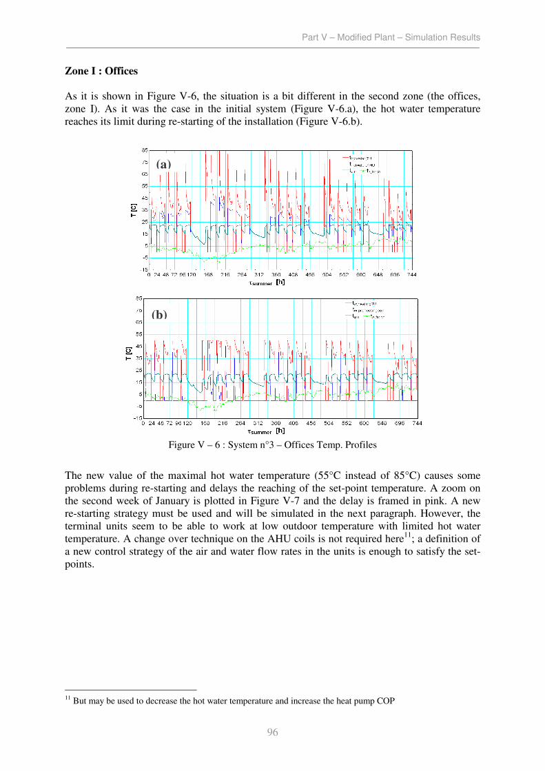
Part V – Modified Plant – Simulation Results
96
Zone I : Offices
As it is shown in Figure V-6, the situation is a bit different in the second zone (the offices,
zone I). As it was the case in the initial system (Figure V-6.a), the hot water temperature
reaches its limit during re-starting of the installation (Figure V-6.b).
The new value of the maximal hot water temperature (55°C instead of 85°C) causes some
problems during re-starting and delays the reaching of the set-point temperature. A zoom on
the second week of January is plotted in Figure V-7 and the delay is framed in pink. A new
re-starting strategy must be used and will be simulated in the next paragraph. However, the
terminal units seem to be able to work at low outdoor temperature with limited hot water
temperature. A change over technique on the AHU coils is not required here11
; a definition of
a new control strategy of the air and water flow rates in the units is enough to satisfy the set-
points.
11
But may be used to decrease the hot water temperature and increase the heat pump COP
(b)
(a)
Figure V – 6 : System n°3 – Offices Temp. Profiles

Part V – Modified Plant – Simulation Results
97
The same conclusion can be made by realizing simulations using the modified set of weather
data.
The summer temperature profiles are not modified; the cooling devices are still supplied with
chilled water at 7°C and are not influenced by the replacement of the air cooled chiller by a
dual condenser chiller.
V.2.3.2. Conclusion
As already supposed, the use of low temperature water (55°C) for heating may cause
problems during winter. The indoor temperature deviates from the set-point temperature and
the room can become too cold for occupants. To ensure the respect of comfort conditions and
to improve the heatpump COP, several adaptations have to be made. These modifications
have been detailed and presented before and are :
- use of change over technique to increase the heat transfer surface (and decrease the
asked hot water temperature),
- envisage adapted re-starting strategies to obtain the wanted temperature during
occupancy periods.
Figure V – 7 : System n°3 – Offices Temp. Profiles (zoom)

Part V – Modified Plant – Simulation Results
98
V.2.4. System n°4 – Heat Pumping & Installation Adaptation
In this case, the both considered adaptations (change over in laboratories AHU and re-starting
strategy in offices) are implemented in the model.
V.2.4.1. Temperature Profiles
Zone III : Laboratories
The January temperature profile is plotted in Figure V-8. Using the change over technique,
the indoor temperature is easily maintained to the set-point (23°C). Indeed, the asked hot
water temperature reaches only 39°C. Knowing that the maximal water temperature is 55°C,
the security margin should be sufficient to ensure the follow-up of the set point in any outdoor
conditions.
Even during cold periods (cf. modified weather data), the set point and the comfort conditions
can be maintained. Moreover, the use of the change over and the functioning at reduced hot
water temperature allows to increase the heat pump performances by decreasing the
condenser exhaust water temperature. Note that, the change over technique has been used
only during heating period. During summer, the installation works in classical mode.
Figure V – 8 : System n°4 – Laboratories Temp. Profiles

Part V – Modified Plant – Simulation Results
99
Zone I : Offices
The January temperature profiles of the offices has been plotted in Figure V-9. The new re-
starting strategy concerns only the terminal units and allows to heat the zone from 20:00 on
Sunday evening till 6:00 on Monday morning (current starting of the installation) and during
cold periods (outdoor temperature below 5°C). To minimize the energy consumption, the
initial ventilation control strategy has been kept and the AHU works only from 6:00 to 20:00
during week. The use of this new control strategy increases slightly the heating demand of the
zone but ensures the follow-up of the set-point since the beginning of the occupancy period.
Of course, the initial re-starting strategy (on Sunday evening, from 17:00 to 20:00) has been
removed and replaced by the new one.
The adaptation seems to be successful : the indoor comfort conditions are guaranteed during
occupancy periods (from 8:00 to 17:00). In Figure V-9, this fact is expressed by the
simultaneity of the decreasing of the asked hot water temperature (corresponding to the
relaxation of the control law) and the beginning of the occupancy periods. The comfort
indices can be computed and give no cold hours (indoor temperature 2°C below the set-point).
The same sort of strategy could be used in the case of very cold periods (cf. modified weather
data). Indeed, in this case, the heating could be maintained 24/24 to avoid the peaks during the
re-starting of the installation12
. The limited number of cold days in our regions should not
make this strategy too expensive.
12
During summer, the same sort of strategy could be used (pre-cooling) and would be cheaper due to the low
price of off-peak electricity.
Figure V – 9 : System n°4 – Offices Temp. Profiles

Part V – Modified Plant – Simulation Results
100
V.2.4.2. Power Profiles
The heating demand, plotted in Figure V-10 (red curve), is mainly satisfied by the heat pump
production (blue-green curve). The interventions of the boilers (as back-boosting devices,
black curve) are limited in amplitude and in frequency. Indeed, the functioning of the boilers
is required when the heat source is unable to provide the sufficient power to allow the heat
pump to produce enough heat on condenser side. At the bottom of the plot, the available
power at the cold source (orange curve) and the really used part of this power (purple curve)
are plotted in negative values.
A zoom of the previous curve is plotted in Figure V-11.
As already said, the boilers intervene only when the cold source power is not sufficient to
allow the satisfaction of the heating demand (red curve) by the Heat Pump. This situation
corresponds to a non null boiler’s power and a used power on heat source side (extracted air)
equal to the maximal available power. The intervention of these “back boosting boilers”
seems limited and quite rare. So, the yearly gas consumption should largely decrease.
Figure V – 10 – System n°4 – Power Profiles
Figure V – 11 : System n°4 – Power Profiles (zoom)

Part V – Modified Plant – Simulation Results
101
V.2.4.3. Consumptions & Performances
The electrical and gas consumptions are detailed in Table V-4.
Table V - 4
Considering these results, the first observation concerns the gas consumption. As expected,
the gas consumption is strongly reduced and passes from 77249 m³ (system n°2) to 1702 m³
(system n°4), which corresponds approximately to a division by 45. Indeed, as shown in
Figure V-12, the larger part (97.7 %) of the heating demand is ensured by the heat pump and
only a small part (2.3 %) is ensure by the gas boilers. Of course, the use of the heat pump as
heating system causes an over-consumption of electrical energy. The global electrical
consumption passes from 1.258 MWh (system n°2) to 1.448 MWh (system n°4). This
increasing is also partially due to the over consumption of the extraction fan caused by the
head loss in the additional recovery coils (about 22053 kWh).
The chosen type of modelling allows us to compute the consumptions in chiller and heatpump
mode separately14
. The heat pump mode consumption is about 148197 kWh without taking
13
Over consumption due to the head loss caused by the installation of additional recovery coils in the extraction
duct.
Electrical
Consumptions Unit Yearly Consumption
Wlights kWh 37461
Wappliances kWh 289474
Wventilation fans kWh 270583
Wheating coils pumps kWh 13110
Wsteam humidifier kWh 428057
Wlaboratories kWh 974330
Woffices kWh 73546
Whot water network pumps kWh 8506
Wcold water network pumps kWh 3837
Wwater networks pumps (secondary) kWh 12343
Wcondenser fans kWh 494
Wcoldrooms kWh 182661
Qcooling demand heatpump kWh 30011
Qheating demand heatpump kWh 732411
Wevaporator pump (primary) kWh 26868
Wcondenser pump (primary) kWh ???
Wheatpump/chiller (compressors) kWh 155839
Wextraction fan over consumption13
kWh 22053
Wpeak hours kWh 775758
Woffpeak hours kWh 672345
Wtotal kWh 1448103
Computed
Consumption Unit Yearly Consumption
Qheating demand boiler kWh 16973
Qgas kWh 18859
Vgas m³ 1702
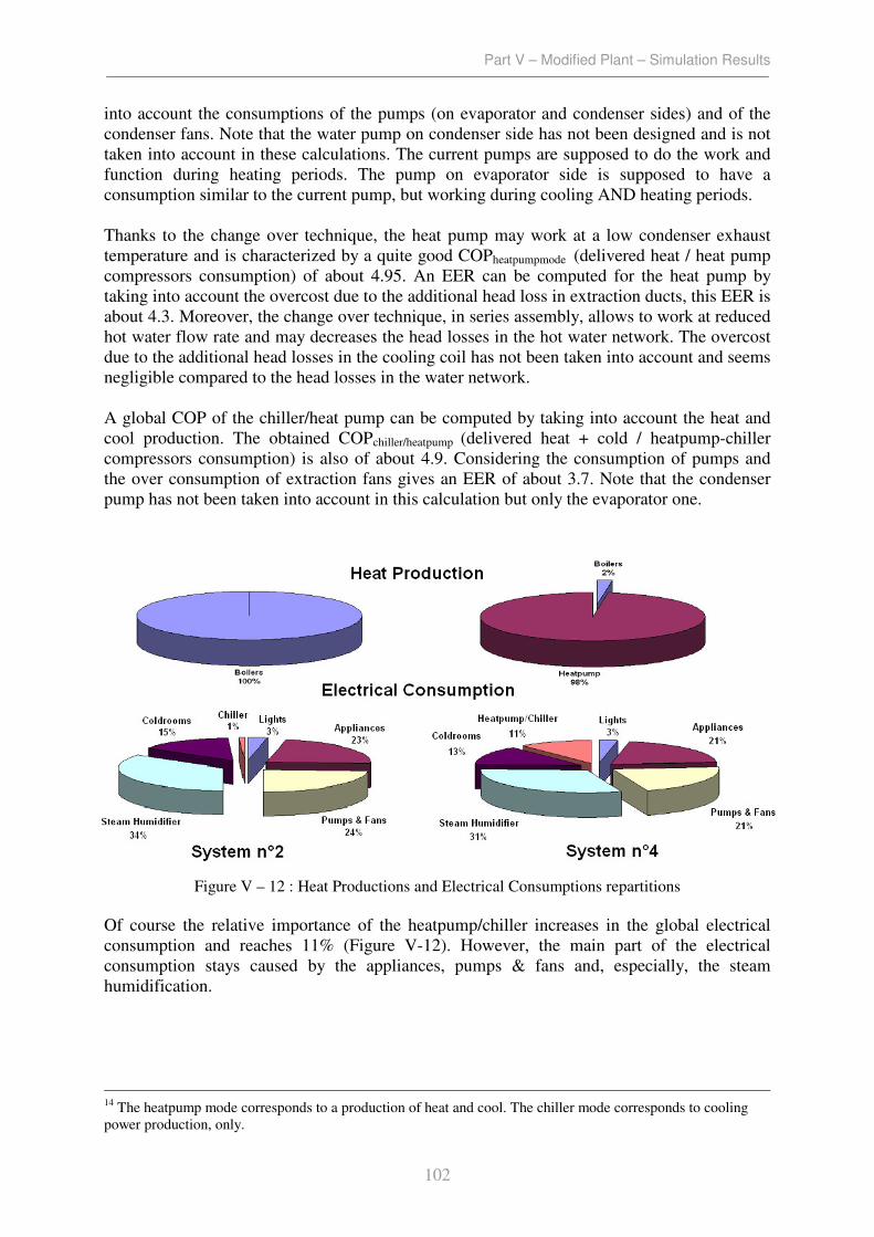
Part V – Modified Plant – Simulation Results
102
into account the consumptions of the pumps (on evaporator and condenser sides) and of the
condenser fans. Note that the water pump on condenser side has not been designed and is not
taken into account in these calculations. The current pumps are supposed to do the work and
function during heating periods. The pump on evaporator side is supposed to have a
consumption similar to the current pump, but working during cooling AND heating periods.
Thanks to the change over technique, the heat pump may work at a low condenser exhaust
temperature and is characterized by a quite good COPheatpumpmode (delivered heat / heat pump
compressors consumption) of about 4.95. An EER can be computed for the heat pump by
taking into account the overcost due to the additional head loss in extraction ducts, this EER is
about 4.3. Moreover, the change over technique, in series assembly, allows to work at reduced
hot water flow rate and may decreases the head losses in the hot water network. The overcost
due to the additional head losses in the cooling coil has not been taken into account and seems
negligible compared to the head losses in the water network.
A global COP of the chiller/heat pump can be computed by taking into account the heat and
cool production. The obtained COPchiller/heatpump (delivered heat + cold / heatpump-chiller
compressors consumption) is also of about 4.9. Considering the consumption of pumps and
the over consumption of extraction fans gives an EER of about 3.7. Note that the condenser
pump has not been taken into account in this calculation but only the evaporator one.
Of course the relative importance of the heatpump/chiller increases in the global electrical
consumption and reaches 11% (Figure V-12). However, the main part of the electrical
consumption stays caused by the appliances, pumps & fans and, especially, the steam
humidification.
14
The heatpump mode corresponds to a production of heat and cool. The chiller mode corresponds to cooling
power production, only.
Figure V – 12 : Heat Productions and Electrical Consumptions repartitions

Part V – Modified Plant – Simulation Results
103
The costs corresponding to the calculated consumptions are presented in Table V-5.
Unit System n°2 System n°4
Wtotal kWh 1258382 1448103
Elec. Cost € 118578 136395
Vgas m³ 77249 1702
Gas Cost € 33238 733
Total Cost € 151816 137128
Saving / year € 14688 Table V - 5
V.2.4.4. Conclusion
The use of a change over technique coupled with reversible heat pumping seems able to
provide good results and performances. Indeed, the use of available heat transfer surface by
using this technique allows to ensure the heating of the considered zones by low temperature
hot water without using expensive adaptations and particular heating devices (as heating
ceiling or walls).
The coupling of the change over technique with the definition of efficient and intelligent re-
starting and control strategies ensures good performances and allows the follow-up of the
comfort conditions.
The natural gas consumption has been largely reduced but not totally cancelled because of the
limitations of the available heat source. The current condensing boilers are used as “back
boosting” devices, when required.
The gas and detailed electrical consumptions have been computed and compared with a
previous scenario (system n°2). Energy and money savings have been quantified. Even if
these adaptations seem to be successful, a detailed economical evaluation of these
money/energy saving measures will be presented hereafter.
Part V – Modified Plant – Simulation Results
104
V.2.5. System n°5 – Thermal Energy Storage
As already said, the installation of a thermal energy storage in the considered system has four
objectives :
1) the storage of the “free” cold energy produced at the evaporator during the functioning
of the heat pump
2) the shifting of the load from day (high outdoor temperature, high electricity price) to
night (lower outdoor temperature, low electricity price), allowing to improve air
condenser performances and money saving,
3) the increasing of the number of hours that chiller operates at high load (and so, high
efficiency)15
,
4) The shifting of the load in heat pump mode also (using the same system to store
heat)16
.
Of course, this thermal storage will be used during summer, when cooling and heating
demands are in alternation.
The design of a cool thermal energy storage system can be based on several criteria :
- average and maximal cooling/heating demands,
- costs of peak and offpeak electrical kWh,
- the cooling/heating capacity of the chiller and the charging power of the storage.
Six tank capacities have been tested : 25,50,75,100,150,200 m³. These volume capacities
correspond to 145,291,436,581,872 and 1163 kWh of “cold energy” by supposing a constant
water temperature variation of 5 K between the supply and the exhaust of the evaporator and a
constant water specific heat of about 4187 J/kg-K.
The tank charging rate is defined as a function of the current level of charge of the storage to
allow a full charging of the tank in 6 hours. Of course, this charging rate can not exceed the
chiller capacity. The choice of a 6 hours period is arbitrary but constitutes a fair and realistic
approximation.
15
The required control system to allow this type of energy saving has not been implemented in the model used. 16
This possibility has not been taken into account in the present work.
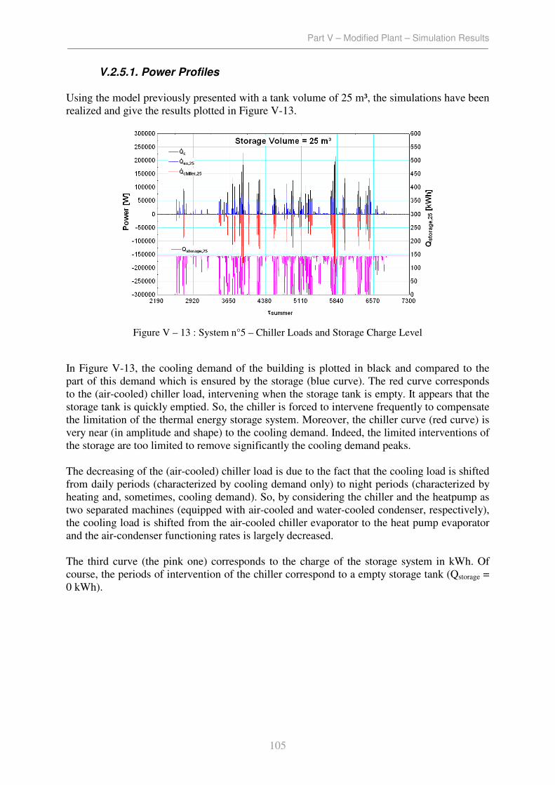
Part V – Modified Plant – Simulation Results
105
V.2.5.1. Power Profiles
Using the model previously presented with a tank volume of 25 m³, the simulations have been
realized and give the results plotted in Figure V-13.
In Figure V-13, the cooling demand of the building is plotted in black and compared to the
part of this demand which is ensured by the storage (blue curve). The red curve corresponds
to the (air-cooled) chiller load, intervening when the storage tank is empty. It appears that the
storage tank is quickly emptied. So, the chiller is forced to intervene frequently to compensate
the limitation of the thermal energy storage system. Moreover, the chiller curve (red curve) is
very near (in amplitude and shape) to the cooling demand. Indeed, the limited interventions of
the storage are too limited to remove significantly the cooling demand peaks.
The decreasing of the (air-cooled) chiller load is due to the fact that the cooling load is shifted
from daily periods (characterized by cooling demand only) to night periods (characterized by
heating and, sometimes, cooling demand). So, by considering the chiller and the heatpump as
two separated machines (equipped with air-cooled and water-cooled condenser, respectively),
the cooling load is shifted from the air-cooled chiller evaporator to the heat pump evaporator
and the air-condenser functioning rates is largely decreased.
The third curve (the pink one) corresponds to the charge of the storage system in kWh. Of
course, the periods of intervention of the chiller correspond to a empty storage tank (Qstorage =
0 kWh).
Figure V – 13 : System n°5 – Chiller Loads and Storage Charge Level

Part V – Modified Plant – Simulation Results
106
The same plots are realized using a thermal storage tank of 75 and 200 m³ (Figure V-14.a and
V-14.b). The others results (for tanks of 50,100 and 150m³) will not be presented but used in
the economical study.
Using a TES system of 75 m³, the chiller load is more largely decreased and the storage
system seems able to reduce the amplitude of peaks. In the case of a 200 m³ storage, the TES
system is able to cover all the cooling demand peaks and allows the shifting of almost the
whole chiller consumption from peak periods to offpeak periods.
Of course, using a TES system, the rate of use of the heat source (extracted air) of the heat
pump is decreased. Indeed, the evaporator load due to the storage charging rate is often
enough to allow the production of the required heat on condenser side. However, this
observation has no real advantage because occurring during summer, when the heat source is
largely sufficient to ensure the heating of the building.
(a)
(b)
Figure V – 14 : System n°5 – Storage Tank Capacity Comparison
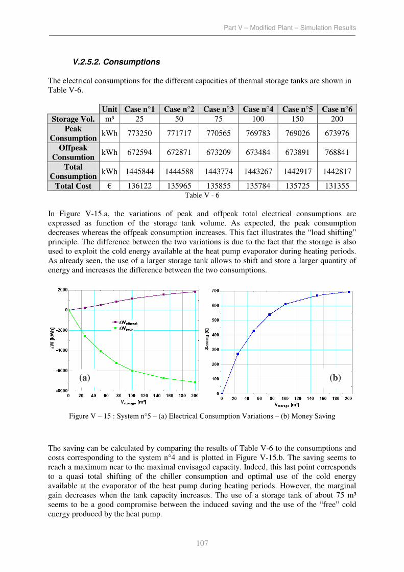
Part V – Modified Plant – Simulation Results
107
V.2.5.2. Consumptions
The electrical consumptions for the different capacities of thermal storage tanks are shown in
Table V-6.
Unit Case n°1 Case n°2 Case n°3 Case n°4 Case n°5 Case n°6
Storage Vol. m³ 25 50 75 100 150 200
Peak
Consumption kWh 773250 771717 770565 769783 769026 673976
Offpeak
Consumtion kWh 672594 672871 673209 673484 673891 768841
Total
Consumption kWh 1445844 1444588 1443774 1443267 1442917 1442817
Total Cost € 136122 135965 135855 135784 135725 131355 Table V - 6
In Figure V-15.a, the variations of peak and offpeak total electrical consumptions are
expressed as function of the storage tank volume. As expected, the peak consumption
decreases whereas the offpeak consumption increases. This fact illustrates the “load shifting”
principle. The difference between the two variations is due to the fact that the storage is also
used to exploit the cold energy available at the heat pump evaporator during heating periods.
As already seen, the use of a larger storage tank allows to shift and store a larger quantity of
energy and increases the difference between the two consumptions.
The saving can be calculated by comparing the results of Table V-6 to the consumptions and
costs corresponding to the system n°4 and is plotted in Figure V-15.b. The saving seems to
reach a maximum near to the maximal envisaged capacity. Indeed, this last point corresponds
to a quasi total shifting of the chiller consumption and optimal use of the cold energy
available at the evaporator of the heat pump during heating periods. However, the marginal
gain decreases when the tank capacity increases. The use of a storage tank of about 75 m³
seems to be a good compromise between the induced saving and the use of the “free” cold
energy produced by the heat pump.
Figure V – 15 : System n°5 – (a) Electrical Consumption Variations – (b) Money Saving
(b) (a)

Part V – Modified Plant – Simulation Results
108
V.2.5.3. Conclusion
The advantages of Thermal Energy Storage system in the considered installation have been
highlighted in the different simulation results. The energy and money savings have been also
quantified. However, even if this last adaptation seems able to provide good results ,an
economic evaluation of this energy/money saving measure must be realized and is presented
below.
It must be noted that the reference weather data is characterized by a quite fresh summer and
that potential of a TES system could increase in the case of a warmer summer. So, it is
allowed to suppose a better use of the TES potential in reality and the capacity of the tank
cannot be designed by only considering the presented results. However, a capacity of 75m³ is
conserved in the economical calculation.

Part V – Modified Plant – Simulation Results
109
V.4. Economical Aspect
V.4.1. Initial Investment and costs definition
As already said, the two last improvements (systems n°4 and n°5) will be now compared to
the second system in a economical way. First, the values of the different investments have to
be estimated. These values are presented in Table V-7.
System n°4
Dual Condenser Chiller/HeatPump [€] 50000
Piping and pumps 10000
Re-starting strategy Adaptation [€] 0
Additional Recovery Coils [€] 10000
Installation [€] 20000
Total Investment [€] 90000
System n°5
Thermal Energy Storage System [€/kWh
storage]17
6 – 21
Table V - 7
Excepted the electricity and gas costs, no operation cost is taken into account. The Thermal
Energy Storage system price is given by Roth et al. ([19], 2006).
V.4.2. Evaluation Methods
Considering these estimated costs, three methods can be used to evaluate the potential money
saving :
- the Payback Time method (PBT),
- the Net Present Value Method (NPV),
- the Internal Rate of Return method (IRR).
The first method is used to compute the payback time without taking into account the
variations of the costs, and values of cash flows with the time. The second method is used to
compute the evolution of the cash outflows and inflows and their influence on the payback
time. The third method gives an information on the quality of the investment and allows to
compare it with other investment (for example).
These economical calculations are often realized in the case of economic evaluation of energy
saving measures (Pilavachi et al., 2007).
V.4.2.1. Payback Time Method
The payback time method is a little bit more basic but can give easily an estimation of the
return on investment time and is expressed by the report between the initial investment and
the yearly estimated cash flow.
17
For a temperature variation of 5K

Part V – Modified Plant – Simulation Results
110
V.4.2.2. Net Present Value Method
The Net Present Value (or NPV) approach describes a method to value a project using the
concepts of the time value of money. All future cash flows are estimated and discounted to
give them a present value (the Discounted Present Value, DPV).
The equation V4.1. express the value of the discounted present value.
Where DPV is the discounted present value of the cash flow CF
CFn is the net cash flow of year n (inflows – outflows)
k is the discount rate, function of the interest rate, the risk of the investment and the
current market
T is the number of years for which the economic evaluation is asked (generally equal
to the investment’s economic lifetime).
The net present value is computed by comparing the discounted present value to the initial
investment (INV, Eq. V.4.2.). The considered investment should be realised only if NPV > 0
after an acceptable number of years. This number of years correspond to the return on
investment time (also called “payback time”).
In our case, the net cash flow is the difference between the saving due to the decreasing of the
gas consumption and the overcost due to the increasing of the electrical consumption. These
two terms vary as a function of time because of the variations of the cost of energy. The
electricity cost is supposed to increase of 1 to 3% per year. The natural gas cost is supposed to
increased of 3 to 6% per year.
V.4.2.3. Internal Rate of Return Method
The IRR evaluation method aims at the determination of the discount rate p that renders the
present value of future discounted net cash flows of an investment equal with the initial cash
outflow (initial investment). The IRR is this discount rate, rendering the examined investment
marginal and constituting the higher interest that can be paid by an investor for finding the
capital that is required for an investment. So, a project is a good investment if its IRR is
greater than the rate of return that could be earned by alternative investments. The discount
rate (IRR) can be determined from the equation V.4.3.
Where INV is the initial investment
p is the Internal Rate of Return
∑=
+=
T
1nn
n
)k1(CFDPV (V.4.1.)
DPVINVNPV +−= (V.4.2.)
∑=
++−=
T
1nn
n
)p1(CFINV0 (V.4.3.)

Part V – Modified Plant – Simulation Results
111
V.4.3. Economic Evaluation of System n°4
Using the simple PBT method, the calculation of the payback time gives, approximately, a
duration of about 6.1 years.
In the Net Present Value Method, three cases have been envisaged : an optimistic one, a
pessimist one and an average one. These cases are characterized by different values of the
discount rate, the variation rate of energy cost, etc (Martin, 2006). These values are shown in
Table V-8.
Optimistic case Average case Pessimist case
igas 6 % 4.5 % 3 %
ielectricity 1 % 2 % 3 %
kdiscount 6 % 8 % 10 % Table V - 8
Obviously, the optimistic case corresponds to an important increasing of the natural gas cost
and a reduced increasing of the electricity cost. These rates give an important increasing of
the saving years by years. The pessimist case corresponds to similar variations rates of
energies costs. The discount rate is very hard to determine. However the current average
values varies around 8%.
The evolutions of cash inflows and outflows are plotted in Figure V-16.a. These evolutions
bring to the results shown in Figure V-16.b.
As shown in Figure V-16.b, the payback time is included between 5 and 8 years. The average
hypotheses correspond to a payback time of about 6 years. These values seems to be
reasonable and the investment could be quickly profitable.
The IRR has been computed and varies between 4 and 9%. The average hypotheses
correspond to a IRR of about 6.5%. This result is quite good comparing to the current rate of
interest.
Figure V – 16 : System n°4 – (a) Cash Inflows and Outflows – (b) Net Present Value
(a)
(b)

Part V – Modified Plant – Simulation Results
112
V.4.4. Economic Evaluation of System n°5
For this calculation, a TES tank of 75m³ has been chosen and corresponds to an initial
investment varying between 2616 and 9159 €. An average initial investment of about 5900 €
has been chosen for the calculations.
This time, using the PBT method, the calculation of the payback time gives about 11 years.
The NPV calculation is also made and, using the three sets of parameters (optimistic,
pessimist and average), gives the results plotted in Figure V-17 (a and b).
As shown in Figure V-17.a, the increasing of the inflow is quite important due to the
increasing of the electrical energy cost. This variation can reach 80 % in the optimistic case.
However, considering the high initial investment and the reduced yearly inflow (due to
electrical energy saving), the payback time is very long and reaches the economic lifetime of
the system (about 20 years). This is due to the fact that the increasing rate of the electricity
price and the inflation rate are comparable. The method gives payback times included
between 16 and 20 years.
Obviously the IRR is very bad and varies between 0.4 and 1.1 %.
Considering the obtained values for PBT and IRR, this last retrofit opportunity does not seem
to be profitable in the considered hypotheses.
Figure V – 17 : System n°5 – (a) Cash Inflows and Outflows – (b) Net Present Value
(a) (b)
Part V – Modified Plant – Simulation Results
113
V.4.5. Conclusion
A classical and complete economic calculation has been realized. The main retrofit
opportunity (system n°4) has been compared to the system n°2 in terms of money saving. The
last system envisaged (use of thermal energy storage) has been compared to the system n°4.
The main retrofit opportunity (reversible heat pumping), giving already good energetic
results, gives good economic results and seems to be profitable after a short number of years
(between 5 and 8 years).
The last retrofit opportunity allows a limited reduction of electrical consumption. This poor
performance is partially due to the fact that the cooling demand of the building is already
limited (using the considered weather data set). Moreover, the importance of the initial
investment and the limited possibility of money saving does not allow to make the
improvement quickly profitable. Indeed, the return on investment is very slow and a real
money saving appears only after an important number of years (in the considered hypotheses).
However, the results presented here must be moderated. The real energy/money saving caused
by the use of the one or the both systems depends directly on the weather. Indeed, a very cold
winter could be characterized by a more important intervention of gas boilers as back
boosting device because of the limitations of the heat source of the heat pump. In the other
hand, the saving due to load shifting during a warmer summer could be more important and
could make this retrofit opportunity more profitable.

Part V – Modified Plant – Simulation Results
114
V.5. Environmental Aspect
In study of the development and the implementation of sustainable technologies, the
calculation of CO2 emissions must be realized. Indeed, in addition to the potential money
saving due to the use of a heat pump instead of gas boilers, the aims of the project are also the
realization of a more sustainable and clean HVAC installation and a better use of primary
energy. Knowing the emissions of CO2 per kWh of primary energy consumed, the calculation
of yearly CO2 emissions is easy.
The following values (Table V-9) are based on averages, function of the quality and the
characteristics of the Belgian power plants and are given by the Walloon region government
(Energie Plus, 2006). These emissions are function of the period (day/night) and the months.
An average value is given for the emissions due to the gas consumption but could vary as a
function of the quality of the combustion or of the burned natural gas.
Emissions due to the Electrical Consumption (kgCO2/kWh)
Period n°1 (November to February)
Peak hours 0.335
Offpeak hours 0.269
Period n°2 (July and August)
Peak hours 0.342
Offpeak hours 0.273
Period n°3 (September to October and March to June)
Peak hours 0.328
Offpeak hours 0.264
Emissions due to the gas consumption (kgCO2/kWh)
0.198 Table V - 9
The emissions due to the electrical consumption must be corrected using a coefficient (Low
Voltage Consumer Factor) of about 1.109. The results are presented in Table V-10.
Unit System
n°1
System
n°2
System
n°4
System
n°5
Peak Cons. kWh 1264024 1258382 1448103 1443267
CO2 Emissions kg CO2 424121 422198 478792 477181
Gas Cons. m³ 76814 77249 1702 1702
Gas Energy Cons. kWh 850958 855774 18859 18859
CO2 Emissions kg CO2 168490 169443 3734 3734
Total CO2 Emissions kg CO2 592611 591641 482526 480915
Table V - 10
As shown in Table V-10, the first modification (modification of the recovery strategy) causes
a small reduction of CO2 emissions (0.97 T CO2/year) in addition to the small benefit
(360€/year). However, this adaptation does not require many investment except the
implementation of an additional control law in the BEM software.
The second modification (use of a reversible heat pump for cooling & heating) causes a larger
reduction of yearly CO2 emissions (116.5 T CO2/year) for the considered weather data set.

Part V – Modified Plant – Simulation Results
115
This decreasing is significant and important. As it was the case for the economical aspect, the
increasing of the electrical consumption is more than balanced by the (quasi) cancellation of
the natural gas consumption. Indeed, the increasing of the electrical consumption causes an
over-production of CO2 of about 56.6 T CO2 / year, but, these emissions are totally balanced
by the reduction of CO2 emissions due to the gas consumption (165.7 T CO2/year) and the
global yearly emissions are reduced of about 109 T CO2/year.
However, the yearly CO2 emissions stay quite high. These emissions are mainly due to the
electrical consumption of the steam humidifiers and of the appliances. These consumptions
bring other retrofit opportunities and should be reduced to by a rationalization work of the
consumptions and, maybe, by the installation of a cheaper (and cleaner) humidification
system.
As already seen, the addition of a thermal energy storage system does not cause significant
electrical consumption (and so emission) reduction but, mainly, a load shifting from peak to
offpeak periods (from day to night).
The same observations can be made by looking to Figure V-18.
Figure V – 18 : CO2 emissions comparison
Part V – Modified Plant – Simulation Results
116
V.6. Conclusions
Five HVAC system configurations have been presented and compared. The first one
corresponds to the actual installation. The four others correspond to the proposed adaptations
and modifications.
The first retrofit opportunity (system n°2), concerning the recovery strategy, seems
successful; it allows a significant energy saving thanks to the removal of a energy wasting.
This adaptations is supposed free: it only requires a modification of the control laws
implemented in the BEM software.
The second retrofit opportunity (system n°3) is based on the use of reversible heat pumping to
satisfy the heating and cooling demands of the building. The large quantity of extracted air is
used as heat source for heat pumping. The actual air cooled chiller is replaced by a new
machine equipped with air cooled and water cooled condensers. This new installation, is still
able to provide chilled water at 7°C, but also ensures the hot water (at 55°C) production. The
use of this low temperature hot water may cause problems in the follow up of the set points
during winter.
The third retrofit opportunity (system n°4) is based on the previous one but used several
adaptations to make the installation able to satisfy the heating demand and to ensure the
follow up of the set points during winter. In the offices, an adaptation of the re-starting
techniques is sufficient to satisfy to the comfort conditions during occupied periods. In the
laboratories, a “change over” technique is used to allow the functioning of the heating coils
(installed in Air Handling Units) with low temperature hot water. This technique benefits of
the already installed and available heat transfer surfaces (as cooling coils) and uses them as
additional heating coils. The series assembly of the two coils is chosen. The coupling of these
two adaptations (modification of re-starting strategy and change over technique) allows the
installation to function with low temperature hot water and to ensure the respect of comfort
conditions.
The fourth retrofit opportunity (system n°5) is based on the previous one, but with addition of
a cool thermal energy storage tank. This storage tank is used to allow a shifting of the heating
or cooling load from peak to offpeak hours and also to recover cool energy during heating
periods.
An economical evaluation of the two last retrofit opportunities (systems n°4 and 5) has been
realized and shows the money saving and the payback time of the two systems. The first one,
seems to be successful and gives a payback time of about 6 years. The second one does not
give such good results and is not profitable in the considered hypotheses.
The environmental aspect has also been approached. The replacement of the classical heating
systems (natural gas condensing boilers) by a heat pumping system allows a significant
reduction of CO2 emissions.

Conclusion
117
CONCLUSION
First, a pre-audit of the actual installation has been made. Basing on measured natural gas and
electrical consumptions, several hypotheses have been made about potential energy wasting
and possible retrofit opportunities. By defining heat transfer coefficients of the building’s
envelope, natural gas consumption has been explained thanks to the thermal signature. Actual
Electrical consumption has also been detailed and partially explained.
Simulation models, implemented on EES (Engineering Equation Solver, © F-Chart Software),
have been developed and used to simulate the thermal behaviour of the studied building and
the coupled HVAC system. The dynamic building model is based on a simplified R-C
network, specially conceived to correspond to commercial buildings’ structure. The global
static HVAC model is composed of distinct models of Air Handling Units, Terminal Units,
chillers, heat pumps, boilers, etc. During the modelling phase, some assumptions have been
made on the building’s envelope and the HVAC system’s components. A typical weather data
set has been used for simulations.
The results given by the developed models have been compared and are in good accordance
with the measured electricity and gas consumptions.
The main retrofit opportunity is the use of reversible heat pumping, with extracted air as heat
source and hot water network or air cooled condenser as heat sink, to satisfy the heating and
cooling demands of the building. Other smaller adaptations, as defining a new recovery
strategy to avoid energy wasting or using a cool thermal energy storage system to allow load
shifting, have also been modelled and simulated.
The advantages of a heat pump system coupled to a change over technique have been
highlighted. Indeed, these two techniques allow to use low temperature hot water produced by
a classical heat pump to heat a building using classical heating devices as air handling units or
terminal units heating coils. No specific heating device (as heating ceiling/floor) is required,
thanks to the change over technique. Moreover, this type of adaptation is not always required
and a simple modification of the ventilation strategy may allow to use a heat pump instead of
boilers to produce hot water.
An economical evaluation of these retrofit opportunities has been made. Payback times and
profitability coefficients have been computed. The installation of the heat pump and the
required adaptations (change over technique and modified re-starting strategies) are
successful and characterized by a quite short payback time. The use of cool thermal storage
did not give such good economical results.
The environmental aspect has also been approached and CO2 emissions have been computed
for each possibility. The reduction of yearly CO2 emissions due to the use of heat pumping
instead natural gas combustion is significant (about 18% of the initial emissions). This
calculation is based on the average emissions characterizing the Belgian electrical power
plant.

Conclusion
118
Other retrofit opportunities should be discussed in the future :
1) the replacement of electrical steam humidifiers by cheaper and cleaner humidification
devices as clean water pulverization, for example,
2) the decreasing of ventilation rate during unoccupied periods,
3) the use of extraction duct’s coils as heat sink to avoid the fans consumptions of the air
cooled condenser,
4) the use of an additional heat source (as the ground) for heat pumping to remove
completely the natural gas consumption,
the use of stratified thermal energy storage to maximize the benefits brought by the use of a
reversible heat pumping system and to minimize primary energy consumption.
References
119
REFERENCES
André, Ph., Lebrun, J., Adam, C., Aparecida Silva, C., Hannay, J., Lemort, V. et al. (2006a) A
contribution to the audit of an air-conditioning system : modelling, simulation and
benchmarking. Proceedings of the 7th
International Conference on System Simulation
in Buildings, Liège, Belgium. Liège : Les Editions de l’Université de Liège.
André, Ph., Lebrun, J., Adam, C., Georges, B., Lemort, V., Teodorese, V. (2006b) From
model validation to production of reference simulations : how to increase reliability
and applicability of building and HVAC simulation models. Proceedings of the 7th
International Conference on System Simulation in Buildings, Liège, Belgium. Liège :
Les Editions de l’Université de Liège.
Aparecida Silva, C., Hannay J., Lebrun, J. (2007) Example of pre-audit of an air conditioning
system. IEA-ECBCS Annex 48 – Work Report. University of Liège.
Architecture and Climate Department – Catholic University of Louvain (2006) Energie Plus :
Conception et rénovation énergétique des bâtiments tertiaires. [Software]. Louvain-la-
Neuve : Architecture et Climat. Tiré de http://mrw.wallonie.be/energieplus/script.htm
As built file. Internal Company Document (2003).
ASHRAE (2004) 2004 ASHRAE Handbook-HVAC Systems and Equipment. Atlanta:
American Society of Heating Refrigerating and Air-Conditioning Engineers, Inc.
ASHRAE (2005) 2005 ASHRAE Handbook-Fundamentals. Atlanta: American Society of
Heating Refrigerating and Air-Conditioning Engineers, Inc.
Braun, J.E., Klein, S.A., Mitchell, J.W. (1989) Effectiveness Models for Cooling Towers and
Cooling Coils. ASHRAE Transactions, (95), 164-174.
Dorgan, C.B., Linder, R.J., Dorgan, C.E. (1999) Chiller Heat Recovery Application Guide.
Atlanta : American Society of Heating, Refrigerating and Air-Conditioning Engineers,
Inc.
Incropera, F.P., DeWitt, D.P. (1996, 4th
ed.) Fundamentals of Heat and Mass Transfer. John
Wiley & Sons. ISBN 0-471-30460-3
Lebrun, J., Ding, Xin, Eppe, J.-P., Wasacz, M. (1990) Cooling Coil Models to be used in
Transient and/or wet regimes. Theoretical Analysis and Experimental Validation.
Proceedings of the 3rd
International Conference on System Simulation in Buildings,
Liège, Belgium. Liège : Les Editions de l’Université de Liège
Lebrun, J.(2005) Machines et systèmes thermiques : notes de cours : cours MECA0006-1.
University of Liège.
References
120
Lebrun, J., André, Ph., Hannay, J., Aparecida Silva, C. (2006a) Example of audit of an air
conditioning system. Proceedings of the Klimaforum Conference, Godovic, Slovenia.
Lebrun, J.(2006b) Utilisation rationnelle de l’énergie, Climatisation des bâtiments et des
véhicules : notes de cours : cours MECA0034-1. University of Liège.
Lebrun, J., André, Ph., Aparecida Silva, C., Hannay, J., Lemort, V., Teodorese, V. (2006c)
Simulation of HVAC systems : development and validation of simulation models and
examples of practical applications. Proceedings of the Mercofrio 2006 Conference,
Porto Alegre, Brazil.
Lebrun, J., Bertagnolio, S., Aparecida Silva, C., Hannay, J. (2007a) Heat pumping and
reversible : air conditioning first case study results. Proceedings of the Heat Transfer
in Components and Systems for Sustainable Energy Technologies, Heat SET 2007
Conference, Chambery, France.
Lebrun, J., Bertagnolio, S., Aparecida Silva, C., Hannay, J. (2007b) Retrofitting proposals
and modelling : First Belgian Case Study. IEA – ECBCS Annex48 Work Report,
University of Liège.
Lemort, V., Cuevas, V., Lebrun, J. (2007) Towards a more easy-to-use cooling coil model.
Paper submitted to be presented and published as an ASHRAE Transaction.
Martin, C. (2006) Evaluation de la rentabilité d’un projet d’investissement : notes de cours :
Formations Responsables Energie. Institut Bruxellois pour la Gestion de
l’Environnement. Tiré de http://www.ibgebim.be.
Ngendakumana, Ph. (2006) Echangeurs de chaleur, aspects fondamentaux et constructifs :
notes de cours : cours MECA 0447-1. University of Liège.
Pilavachi, P., Chletsis, A., Nikolaidis, Y. (2007) Economic Evaluation Of Energy Saving
Measures In Buildings. Proceedings of the Heat Transfer in Components and Systems
for Sustainable Energy Technologies, Heat SET 2007 Conference, Chambery, France.
Roth, K. , Zogg, R., Brodrick, J. (2006) Cool Thermal Energy Storage. ASHRAE Journal, 48,
94-96.