Embed Size (px)
Citation preview
Text-Independent Voice Conversion
David Sundermann
Der Fakultat fur Elektrotechnik und Informationstechnikder Universitat der Bundeswehr Munchen
zur Erlangung des akademischen Grades eines
Doktor-Ingenieur(Dr.-Ing.)
vorgelegte Dissertation

Abstract
This thesis deals with text-independent solutions for voice conversion. It first introducesthe use of vocal tract length normalization (VTLN) for voice conversion. The presentedvariants of VTLN allow for easily changing speaker characteristics by means of a few trainableparameters. Furthermore, it is shown how VTLN can be expressed in time domain stronglyreducing the computational costs while keeping a high speech quality.
The second text-independent voice conversion paradigm is residual prediction. In par-ticular, two proposed techniques, residual smoothing and the application of unit selection,result in essential improvement of both speech quality and voice similarity.
In order to apply the well-studied linear transformation paradigm to text-independentvoice conversion, two text-independent speech alignment techniques are introduced. One isbased on automatic segmentation and mapping of artificial phonetic classes and the otheris a completely data-driven approach with unit selection. The latter achieves a performancevery similar to the conventional text-dependent approach in terms of speech quality andsimilarity. It is also successfully applied to cross-language voice conversion.
The investigations of this thesis are based on several corpora of three different languages,i.e., English, Spanish, and German. Results are also presented from the multilingual voiceconversion evaluation in the framework of the international speech-to-speech translationproject TC-Star.

Acknowledgments
My entire and perfect appreciation is due Prof. Dr. Harald Hoge. Over the four years ofthis project and before, he played the outstanding roles of my teacher, my supervisor, mycolleague, my financial backer, my patron, and my friend. Without him, most of the lastyears’ exciting work would not have been possible.
This thesis brought me and my blessed family around the world: We lived in the Nether-lands, in Barcelona, Munich, Los Angeles, and New York City, calling for a lifestyle thatwas only possible due to the extraordinary flexibility and absolute endorsement of my wifeChristiane Sundermann-Oeft and the enthusiasm for aviation and foreign languages of mydaughters Nele Theophanu, Hannah Eulalia, and Kara-Lailach Igone.
Many researchers supported this dissertation scientifically, financially, and ideally – I amwholeheartedly indebted to Profs. Drs. Antonio Bonafonte, Julia Hirschberg, Shri Narayanan,and Hermann Ney for giving me the opportunity to work in their distinguished researchlaboratories. Further services for the successful completion of this work were rendered bymy former teacher Prof. Dr. Rudiger Hoffmann kindly serving as reviewer of this work, byDr. Jaka Smrekar who provided valuable mathematical assistance, by Dr. Renko Geffarthproofreading the manuscript, and by my parents Sabine and Dr. Uwe Sundermann.
New York City, October the 28th, 2007

Contents
1 Introduction 1
1.1 Text-Independent and Cross-Language Voice Conversion . . . . . . . . . . . 21.2 Application Areas of Voice Conversion . . . . . . . . . . . . . . . . . . . . . 21.3 Objectives and Contributions . . . . . . . . . . . . . . . . . . . . . . . . . . 3
2 State of the Art 5
2.1 Text-Independent Voice Conversion . . . . . . . . . . . . . . . . . . . . . . . 52.2 Cross-Language Voice Conversion . . . . . . . . . . . . . . . . . . . . . . . . 72.3 The Speech Production Model . . . . . . . . . . . . . . . . . . . . . . . . . . 82.4 Changing Voice Quality: VTLN, Linear Transformation, and Residual Pre-
diction . . . . . . . . . . . . . . . . . . . . . . . . . . . . . . . . . . . . . . . 152.5 Evaluation Metrics for Voice Conversion . . . . . . . . . . . . . . . . . . . . 23
3 VTLN-Based Voice Conversion 27
3.1 Parameter Training . . . . . . . . . . . . . . . . . . . . . . . . . . . . . . . . 273.2 A Piece-Wise Linear Warping Function with Several Segments . . . . . . . . 283.3 Frequency Domain vs. Time Domain VTLN . . . . . . . . . . . . . . . . . . 303.4 On Generating Several Well-Distinguishable Voices . . . . . . . . . . . . . . 40
4 Residual Prediction 49
4.1 Residual Smoothing . . . . . . . . . . . . . . . . . . . . . . . . . . . . . . . . 494.2 Unit Selection . . . . . . . . . . . . . . . . . . . . . . . . . . . . . . . . . . . 554.3 Applying VTLN to Residuals . . . . . . . . . . . . . . . . . . . . . . . . . . 59
5 Text-Independent and Cross-Language Voice Conversion 63
5.1 Automatic Segmentation and Mapping of Artificial Phonetic Classes . . . . . 645.2 Text-Independent Voice Conversion Based on Unit Selection . . . . . . . . . 685.3 From Text-Independent to Cross-Language Voice Conversion . . . . . . . . . 725.4 The Speech Alignment Paradox . . . . . . . . . . . . . . . . . . . . . . . . . 77
6 Achievements and Conclusions 93
A Appendix 95
A.1 TC-Star . . . . . . . . . . . . . . . . . . . . . . . . . . . . . . . . . . . . . . 95A.2 Corpora . . . . . . . . . . . . . . . . . . . . . . . . . . . . . . . . . . . . . . 95A.3 Proofs . . . . . . . . . . . . . . . . . . . . . . . . . . . . . . . . . . . . . . . 97

1 Introduction
Voice conversion is a technology that transforms characteristics of a source voice to those of atarget voice. This means, we are given a source voice (in terms of recorded speech) and wantit to be converted to another voice, the target voice whose characteristics are given either byrecorded speech as well or by more general descriptors as the gender or age of the speaker,parameters as mean fundamental frequency or speaking rate, or just by the requirement ofbeing sufficiently different from the source.
In addition to this vague definition of the target, we face vagueness in what we refer toas voice characteristics. Here we have two different levels:
• voice quality (or timbre, the set of segmental cues) describes the voice’s sound influ-enced by formant locations and bandwidths, spectral tilt, and the contribution of thevoice excitation by the vocal folds [Childers & Lee 91],
• prosody (or the set of supra-segmental cues) is related to the style of speaking and in-cludes phoneme duration, evolution of fundamental frequency (intonation) and energy(stress) over the utterance [Horne 00].
This dissertation deals with two specific tasks out of the set of possibilities introduced above:
1. A source voice given by recorded speech is to be transformed so that the convertedvoice sounds different from the source in a specific way (e.g. change of gender).
2. A source voice given by recorded speech is to be transformed so that the convertedvoice sounds similar to a target voice given by recorded speech as well.
As will be discussed below, the voice conversion technology described in this disser-tation is applied to both the intra-lingual and the cross-language task where sourceand target voice use different languages. Since prosody is highly language-dependent[Dutoit 93, Boudelaa & Meftah 96, Barbosa 97, Zhu & Zhang+ 02], it is a very hard taskto convert a speaker’s prosodical characteristics across languages1. This is the reason foromitting prosodical conversion in this work. The only prosodical property to be transformedis the mean fundamental frequency having strong influence on the perception of a voice asshown in Section 3.4. Since voice quality seems to be much more independent of the languagethan prosody, this dissertation focuses on the transformation of voice quality2.
Approaches presented in this thesis are evaluated using state-of-the-art error measuresas discussed in Section 2.5. They deal with the success of voice conversion, i.e. with the
1Recent investigations in the framework of speech-to-speech translation use prosodical features of the sourceto produce a more natural target prosody across languages [Aguero & Adell+ 06]. However, here, thetarget is synthetic speech produced by a text-to-speech system, and the proposed approach cannot beapplied to natural speech, since it does not aim at detecting parallelisms between source and target.
2There is evidence that also certain voice quality aspects vary between languages [Braun & Masthoff 02],but this effect is much weaker than the language dependence of prosody.
1 Introduction
similarity of converted and target voice, as well as with the overall quality of the convertedvoice. The present work reports on both types of measures, those based on human listeningtests and also automatic ones.
1.1 Text-Independent and Cross-Language Voice
Conversion
Looking at task 2 introduced above, there is no statement about the properties of therecorded speech being required. Obviously, characteristics as how much speech is available,whether it is based on phonetically balanced text, whether the recording is of high quality(in terms of signal-to-noise ratio, sampling frequency, and quantization), and whether thespeakers are professional, are of vital importance for a successful voice conversion. However,as we will learn in Section 2.1, the most crucial point is that both source and target speech aretime-aligned. Such an alignment can be produced by means of well-investigated techniqueswhen both speech samples involved are based on the same text. This case is referred toas text-dependent as opposed to the case of the texts being different; this is called text-
independent.The task becomes even more complicated if the involved speech samples’ languages
differ. Here, we mostly face different phoneme sets, thus we are unable to find an appropriatetime alignment to phonemes that are missing in the other phoneme set. Therefore, one alsodistinguishes between intra-lingual and cross-language voice conversion.
1.2 Application Areas of Voice Conversion
In literature, a vast number of applications for voice conversion is given. Obviously, only afew of them were ever carried out. Therefore, the author restricts his considerations to themost popular ones:
A. Definitely, the most important application of voice conversion is the use as a mod-ule in text-to-speech synthesis where we want to change the standard speaker’svoice characteristics towards a well-defined target speaker [Kain 01]. This is usedto rapidly adapt, personalize, or corporatize synthesized voices, e.g. in dialog systems[Fischer & Kunzmann 06].
B. Moreover, voice conversion has been applied to normalizing high quality speechdatabases to enlarge the amount of available speech data to build a concatenativespeech synthesis system [Eide & Picheny 06].
C. In embedded environments, voice conversion can serve to manipulate voices in sucha way that the original speaker cannot be recognized or the speaker’s gender or ageis changed. Due to computational limitations, conversion algorithms of embeddedsystems focus on manipulating only a few parameters as fundamental frequency andvocal tract length [Sundermann & Ney+ 03b].
D. Cross-language voice conversion has been applied to dubbing tasks in the film andmusic industry [Turk & Arslan 02].
2
1.3 Objectives and Contributions
E. In the framework of speech-to-speech translation, a translated sentence is to be utteredwith the source speaker’s voice [Hoge 02]. Here, in addition to speech recognition,machine translation, and speech synthesis, a text-independent cross-language voiceconversion module is necessary.
F. For people who are speech-impaired or -disabled voice conversion can be a meansleading to more natural and intelligible speech as for persons suffering dysarthria[Hosom & Kain+ 03] or laryngectomy [Nakamura & Toda+ 06].
G. Recently, voice conversion has been applied to speaker normalization for speech recog-nition. In particular, it was used for reducing the Lombard effect describing avoice’s change in noisy environments, in order to improve the recognition performance[Boril & Fousek+ 06].
1.3 Objectives and Contributions
The main objectives of this work are
• to develop a technique for producing a target voice that is sufficiently different fromthe source voice and can be easily controlled by means of few parameters. It is tobe investigated how many well-distinguishable voices can be created from a singlesource voice without affecting the naturalness of the resulting voice. Furthermore, thetechnique is to be optimized in terms of time and memory complexity to be applied inan embedded environment (application C),
• to improve the state of the art of the converted voice’s naturalness and similarity tothe target by investigating residual prediction techniques (applications A, B, D, E),
• to produce solutions to voice conversion that are text-independent which is mandatoryfor its application to speech-to-speech translation (E) and convenient for most of theaforementioned applications (A, B, D, F, G),
• to investigate solutions to cross-language portability that is crucial for applying voiceconversion to speech-to-speech translation (E) and other tasks (D).
The main contributions of this work are
• the application of vocal tract length normalization (VTLN) to voice conversion,
• the generalization of VTLN warping functions by means of a piece-wise linear functionwith several segments which allows for applying dynamic programming to estimate itsparameters,
• to prove that VTLN which is normally applied in frequency domain can be applieddirectly in time domain omitting two Fourier transformations and, hence, may stronglyaccelerate the voice conversion – the author refers to this concept as time domain
VTLN,
• to show that VTLN-based voice conversion is able to produce several well-distinguishable voices (five or more) based on one source voice by varying two pa-rameters (warping factor and mean fundamental frequency),
3

1 Introduction
• two residual prediction techniques (one based on residual smoothing, the other basedon unit selection) that outperform the state of the art in terms of overall speech qualityand similarity to the target,
• a text-independent speech alignment technique based on unit selection that can beused as a preprocessor of conventional (text-dependent) voice conversion techniques,
• to show that the aforementioned text-independent speech alignment technique is ro-bust with respect to the cross-language task and produces higher speech quality thanconventional text-dependent alignment (dynamic time warping).
4
2 State of the Art
Having a look at an excerpt of the call for papers of the world’s largest speech processingconference, Interspeech, held August 2007 in Antwerp, Belgium, one finds, among others,the following research fields:
a. speech coding,
b. speech synthesis,
c. speech recognition,
d. cross-lingual processing,
e. speaker recognition,
f. evaluation and standardization.
This dissertation deals with text-independent voice conversion, a topic positioned betweenall of these fields, borrowing and joining knowledge from all of them and making voiceconversion an interdisciplinary research area. In particular, it loans
• the source-filter model, linear prediction, and residual processing from a,
• acoustic synthesis, the unit selection paradigm, and the approach of pitch-synchronousprocessing from b,
• vocal tract length normalization and the Gaussian mixture model from c,
• the concepts of text-independence and cross-language portability from d,
• linear transformation, vector quantization, and clustering from e,
• the concepts of objective and subjective evaluation as well as several standardized errormeasures from f.
This chapter is to introduce the aforementioned concepts building a bridge to their applica-tion to voice conversion. Furthermore, the respective application’s state of the art in voiceconversion research is briefly presented.
2.1 Text-Independent Voice Conversion
Speech is the human being’s original communication medium. It carries threefold informa-tion:
• segmental information (related to voice quality),
2 State of the Art
• supra-segmental information (related to prosody),
• linguistic information (expressed by the series of phonemes uttered).
The first two of these, segmental and supra-segmental information, are related to voicecharacteristics introduced in Chapter 1, whereas the third is not to be covered under thescope of voice characteristics in this dissertation3. Although linguistic information is notfocus of this work, its presence plays an important role for the following investigations.Most of the state-of-the-art voice conversion techniques which aim at converting a sourcetowards a given target speaker (task 2 of Chapter 1) work in two phases, the training and theconversion phase. In training, speech of both the source and target voices is processed, anduseful information (parameters) is extracted. These parameters are used in the conversionphase to change the voice characteristics of a new source utterance to sound similar to thetarget voice.
When introducing the speech production model in Section 2.3 it will be argued that thevocal tract shape is responsible for both
• the individual sounds (phonemes) produced by the speaker and
• an essential part of the speaker’s voice characteristics related to voice quality.
Voice-quality-related information is extracted by comparing speech data of source and targetspeaker. In doing so, one has to compensate for variations which are due to the phonemesuttered. This compensation can be done by using time-aligned speech, i.e., where bothspeakers produced the same phonemes at exactly the same time.
The easiest way to achieve such an alignment is the text-dependent approach. Here,one uses speech of both involved voices based on the same text (also referred to as par-
allel speech). To produce an exact time alignment, there are standard techniques asdynamic time warping [Rabiner & Rosenberg+ 78], or hidden-Markov-model-based forcedalignment [Young & Woodland+ 93] (which tends to be more exact than dynamic time warp-ing [Inanoglu 03]), or a combination of both [Duxans & Bonafonte 03]. Forced alignmentrequires the underlying text as well as acoustic and language models, i.e., it is language-dependent, as opposed to dynamic time warping which is language-independent.
As argued in Section 1.3, several applications require a text-independent alignment,i.e., the speakers’ utterances are based on different texts (i.e. non-parallel data). Interest-ingly, when the author started his investigations on text independence for voice conversion,to the best of his knowledge, there were no publications dealing with this issue yet. Toclearly distinguish between his work and that of other researchers, he decided to discusshis first contribution, the automatic segmentation and mapping of artificial phonetic classes[Sundermann & Ney 03a], in Section 5.1 and dedicated the current section to another recentwork on text independence of voice conversion.
The automatic segmentation and mapping does not require any phonetic knowledgeabout the considered language, i.e., it is language-independent. This fact is advantageous onthe one hand, since the technique can be applied to arbitrary languages without additionaldata. On the other hand, more information about the phonetic structure of the processedspeech could lead to a more reliable mapping between source and target speech.
3There are indeed opinions partially relating linguistic information (as the speaker’s accent) to voice char-acteristics [Kain 01].
6
2.2 Cross-Language Voice Conversion
Consequently, [Ye & Young 04b] proposed to use a speaker-independent hidden-Markov-model-based speech recognizer to label each frame4 with a state index such thateach source or target speaker utterance is represented by a state index sequence. If the textof these utterances is known, this can be done by means of forced alignment resulting inmore reliable state sequences.
In a second step, subsequences are extracted from the set of target sequences to matchthe given source state index sequences using a simple selection algorithm. This algorithmfavors longer matching sequences to ensure a continuous spectral evolution of the selectedtarget speech frames. The latter are derived from the state indices considering the frame–state mapping delivered by the speech recognizer. The result is two sequences of parallelspeech frames.
2.2 Cross-Language Voice Conversion
The very first investigations on cross-language voice conversion in the beginning of the 1990sfocused on the speech-to-speech translation task [Abe & Shikano+ 90]. At that time, ATR(Advanced Telecommunications Research Institute International in Kyoto, Japan) wherethe authors of the latter paper were working was developing a so-called interpreting tele-
phone. This was the name of a speech-to-speech translation system applied to telephoneconversations. It integrated a cross-language voice conversion module to preserve speakerrecognizability across languages.
This first attempt was based on a codebook mapping that used a discrete representationof the acoustic feature space. To the best of the author’s knowledge, there were no inves-tigations carried out dealing with the technique’s speech quality. [Stylianou & Cappe+ 95]claimed that there were considerable artifacts due to the discreteness of the codebook map-ping approach in order to promote their linear transformation technique, see Section 2.4.2.
Besides, it was not sufficiently shown whether the codebook mapping approach is able tosuccessfully convert voice characteristics. The results reported were based on objective errormetrics that are not standardized and sometimes hardly correlate with the perceptive similar-ity, cf. Section 2.5. Subjective experiments using the described codebook mapping techniquereported successful gender transformation from male to female and 61% successfully trans-formed examples for male-to-male conversion using an ABX5 test [Abe & Nakamura+ 88].Although this approach was text-independent, it did not produce an alignment betweensource and target speech. This is the reason for not considering this technique in Section 2.1.
More than a decade later, Japanese researchers (some of them also at ATR) continuedthe investigations on cross-language voice conversion and applied the linear transformationparadigm introduced in Section 2.4.2 [Mashimo & Toda+ 01]. They avoided the text inde-pendence problem by using bilingual (Japanese/English) speakers as source speakers. Theconversion function was trained on parallel Japanese utterances of source and target speak-ers and applied to English source speech in conversion phase. The only difference to text-dependent intra-lingual voice conversion are the different phoneme sets of source and targetlanguage. The corresponding intra-lingual baseline system described in [Toda & Lu+ 00]achieved a fair speech quality (mean opinion score 2.9) and a conversion performance ofabout 90% on an ABX scale (for these evaluation metrics, see Section 2.5).
4For a definition of the term speech frame, see Section 2.3.1.5For the definition of an ABX test, see Section 2.5.2.
7
2 State of the Art
For projects like the interpreting telephone, TC-Star6, or Minnesang7, the text-dependent solution to cross-language voice conversion is hardly applicable for the followingreasons:
• At least one of the involved speakers would have to speak both source and targetlanguage to apply the text-dependent training.
• However, this would not be the source speaker, since otherwise there were no need forspeech-to-speech translation.
• The target speaker is a synthetic voice generally based on a unit selection concatenativetext-to-speech system involving a large speech corpus (≥ 10h) of a professional andcarefully selected speaker [Black & Lenzo 01]. It would be a severe restriction to thespeaker selection to demand bilingual speakers. If the speech-to-speech translationsystem is used in several languages, one would require either a professional speakingall languages to be converted, or one would have to build a new bilingual voice for alllanguage combinations to be considered.
• The introduction of a new language would mean to build a new text-to-speech voicefrom scratch.
• Since the system is text-dependent, a set of utterances based on a predefined textwould be required by each source speaker who wants to use the system.
All of these drawbacks are to be overcome by the text-independent and cross-language solu-tions discussed in Chapter 5.
2.3 The Speech Production Model
2.3.1 Speech as a Sequence of Frames
Once again, the three types of information carried by human speech are to be consulted:
• segmental information (related to voice quality),
• supra-segmental information (related to prosody),
• linguistic information (expressed by the series of phonemes uttered).
Looking at a single utterance, voice quality can be regarded as constant or, at least, slowlychanging, whereas phonemes change rapidly over time8. To capture all necessary informationof a time-varying speech signal, it is therefore necessary to split the signal into small portions(frames) which themselves can be regarded as stationary. The smaller such a frame is, themore stationary are its contents.
Still, there is a natural lower limit to the frame size coming from the third speechinformation type, the prosody. Prosody covers the evolution of fundamental frequency for a
6See Section A.1.7In the Minnesang project [Spelmezan & Borchers 06], an exhibition’s visitor listens to his voice speaking
a medieval German poem after having uttered a short verse in his mother tongue.8As an example, [Hain 01] reports around 10 phonemes per second for British English spontaneous speech.
8
2.3 The Speech Production Model
typical adult female reaching from 165 to 255Hz and for a typical adult male from 85 to 155Hz[Dolson 94]. Using smaller frames than those given by the signal’s periodicity would meanto lose not only the fundamental frequency but also to reduce the amount of informationcontained in a frame to such a degree that feature extraction methods as linear predictionwould fail, cf. Section 2.3.3. Typically, in speech coding and recognition, frame lengthsbetween 10 and 30ms are used, e.g. 20ms for the GSM and UMTS codecs [Hillebrand 02], and25ms for many speech recognizers, see e.g. [Ney & Welling+ 98] or [Furui & Nakamura+ 06].
For both mentioned fields, speech coding and recognition, state-of-the-art techniquesare based on constant frame lengths [Dharanipragada & Gopinath+ 98], whereas in speechsynthesis, the frame lengths are usually linked to the fundamental frequency (pitch). Thatis, they make use of the pitch-synchronous paradigm which allows for applying standardpitch and duration modification techniques as pitch-synchronous overlap and add (PSOLA)[Charpentier & Stella 86]; for details refer to Section 2.3.4.
Due to the excitation of the voice by the periodically vibrating vocal fold duringvoiced sounds (see Section 2.3.2 for the source-filter model), speech can be regarded apseudo-periodic signal in voiced regions. The pitch-synchronous paradigm is to cut thesignal into frames each of which contains such a period. The automatic detection of thecutting points is referred to as pitch marking [Cheng & O’Shaughnessy 89] which turnsout to be a rather difficult task keeping a number of researchers busy even nowadays[Bernadin & Foo 06, Germann 06, Kotnik & Hoge+ 06, Mattheyses & Verhelst+ 06]. In un-voiced regions, the pitch marks are interpolated between neighbored voiced regions, or con-stant frame durations (e.g. 10ms) are assumed [Black & Lenzo 03].
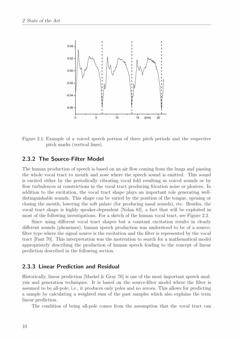
Frequently discussed is the question which cutting point within the pseudo-periodicsignal is the most reliable one while, at the same time, it maximally correlates with theperiodicity of the laryngeal excitation. [Hoge & Kotnik+ 06] found that “the time instantat which the lower margins of the vocal folds are touching each other can be uniquely andconsistently determined on the basis of the speech signal itself. Therefore, [...] the mostnegative peak of the speech signal will be defined as the [...] starting point of each new pitchperiod”. Figure 2.1 shows three periods of a speech signal and the respective cutting pointsaccording to this definition.
At the beginning of his work on voice conversion, the author made use of the algorithmfor “accurately marking pitch pulses in speech signals” by [Goncharoff & Gries 98] which isbased on dynamic programming. In a recent evaluation [Kotnik 06], it was shown that thisalgorithm was clearly outperformed by the Praat algorithm working in the lag (autocorre-lation) domain. Praat was claimed “to be several orders of magnitude more accurate thanthe methods commonly used” according to the algorithm’s creator [Boersma 01].
The Praat software comes along with a voicing detector and only produces pitch marksin voiced signal parts. In unvoiced regions, pitch marks have to be padded as explained above,whereas the Goncharoff/Gries algorithm automatically produces pitch marks for the wholesignal including unvoiced portions. However, for several investigations in this work (as forinstance on PSOLA, cf. Section 2.3.4), it is necessary to be explicitly provided with voicinginformation. Thus, in connection with the Goncharoff/Gries pitch marking algorithm, thevoicing detector used for the Adaptive Multi-Rate speech codec [ETSI 99] was used. Thisalgorithm does not only detect but it also provides a continuous level of voicing 0 ≤ v ≤ 1where v = 0 is completely unvoiced and v = 1 is completely voiced. Such a continuous levelof voicing will be of particular interest for the residual smoothing technique discussed inSection 4.1.
9
2 State of the Art
0 5 10 15 20
-0.06
-0.04
-0.02
0.00
0.02
0.04
t[ms]
Figure 2.1: Example of a voiced speech portion of three pitch periods and the respectivepitch marks (vertical lines).
2.3.2 The Source-Filter Model
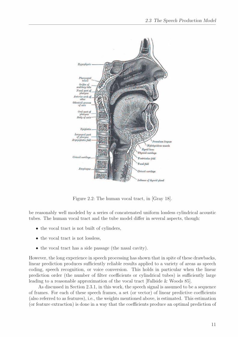
The human production of speech is based on an air flow coming from the lungs and passingthe whole vocal tract to mouth and nose where the speech sound is emitted. This soundis excited either by the periodically vibrating vocal fold resulting in voiced sounds or byflow turbulences at constrictions in the vocal tract producing frication noise or plosives. Inaddition to the excitation, the vocal tract shape plays an important role generating well-distinguishable sounds. This shape can be varied by the position of the tongue, opening orclosing the mouth, lowering the soft palate (for producing nasal sounds), etc. Besides, thevocal tract shape is highly speaker-dependent [Nolan 83], a fact that will be exploited inmost of the following investigations. For a sketch of the human vocal tract, see Figure 2.2.
Since using different vocal tract shapes but a constant excitation results in clearlydifferent sounds (phonemes), human speech production was understood to be of a source-filter type where the signal source is the excitation and the filter is represented by the vocaltract [Fant 70]. This interpretation was the motivation to search for a mathematical modelappropriately describing the production of human speech leading to the concept of linearprediction described in the following section.
2.3.3 Linear Prediction and Residual
Historically, linear prediction [Markel & Gray 76] is one of the most important speech anal-ysis and generation techniques. It is based on the source-filter model where the filter isassumed to be all-pole, i.e., it produces only poles and no zeroes. This allows for predictinga sample by calculating a weighted sum of the past samples which also explains the termlinear prediction.
The condition of being all-pole comes from the assumption that the vocal tract can
10
2.3 The Speech Production Model
Figure 2.2: The human vocal tract, in [Gray 18].
be reasonably well modeled by a series of concatenated uniform lossless cylindrical acoustictubes. The human vocal tract and the tube model differ in several aspects, though:
• the vocal tract is not built of cylinders,
• the vocal tract is not lossless,
• the vocal tract has a side passage (the nasal cavity).
However, the long experience in speech processing has shown that in spite of these drawbacks,linear prediction produces sufficiently reliable results applied to a variety of areas as speechcoding, speech recognition, or voice conversion. This holds in particular when the linearprediction order (the number of filter coefficients or cylindrical tubes) is sufficiently largeleading to a reasonable approximation of the vocal tract [Fallside & Woods 85].
As discussed in Section 2.3.1, in this work, the speech signal is assumed to be a sequenceof frames. For each of these speech frames, a set (or vector) of linear predictive coefficients(also referred to as features), i.e., the weights mentioned above, is estimated. This estimation(or feature extraction) is done in a way that the coefficients produce an optimal prediction of
11
2 State of the Art
the respective frame’s samples. Here, optimality is defined as the minimization of the error,i.e. the differences between the predicted and the actual signal, also referred to as residual.Feeding the residual to the linear prediction model, i.e. filtering the residual by means of theabove coefficients, always gives back the original signal [Smith 07]. Therefore, the residualstands for the excitation and the linear predictive filter for the vocal tract of the source-filtermodel of Section 2.3.2.
The error minimization for estimating the linear predictive coefficients is carried outusing the ancient least squares approach [Gauss 09], according to which the minimization isapplied to the sum of the squared sample differences. [Makhoul 75] shows that this mini-mization can be performed by applying the Levinson-Durbin algorithm [Durbin 60] to theautocorrelation sequence of the frame’s power spectrum.
In addition to linear predictive coefficients, a number of other feature types has beenwidely used for speech processing:
• Line spectral frequencies [Itakura 75]. When being applied to linear-transformation-based voice conversion linear predictive coefficients as defined abovetend to produce artifacts that can be effectively suppressed by converting the coeffi-cients to line spectral frequencies. This is due to their superior interpolation propertiesas compared to other linear prediction representations [Paliwal 95], a fact that is ex-ploited in the linear transformation introduced in Section 2.4.2. An algorithm forconverting linear predictive coefficients to line spectral frequencies and vice versa isgiven e.g. in [Deller & Proakis+ 93].
• Mel frequency cepstral coefficients [Picone 93]. This type of feature provides acompact representation of the speech amplitude spectrum in a form which is anatomi-cally and perceptually motivated. Like in the cochlea, the amplitude spectrum is scaledaccording to the mel scale [Stevens & Volkman+ 37] and filtered by means of a numberof (triangular) overlapping bandpass filters. Now, the discrete cosine transformation isapplied to the list of mel amplitudes finally producing the features which are the ampli-tudes of the resulting spectrum. According to [Ye & Young 04a], mel frequency coeffi-cients, formerly used in the linear transformation framework [Stylianou & Cappe+ 95],are outperformed by line spectral frequencies in terms of speech quality.
• Cubic-spline-interpolated cepstrum [Ye & Young 03]. Here, the logarith-mized spectral amplitudes are resampled to a certain number of frequency pointswhich then are transformed to the cepstral domain. A similar feature typewas used by the author in an investigation on text-independent voice conversion[Sundermann & Bonafonte+ 04a], but [Ye & Young 04a] themselves worked out thatthese features produce a lower speech quality than line spectral frequencies.
For these reasons, line spectral frequencies will be used as features in this work unlessotherwise noted.
2.3.4 Pitch-Synchronous Overlap and Add
Now, having introduced linear prediction as a principal feature extraction method, the farend of frame-based speech processing, the acoustic synthesis, is to be discussed. Purposeof the acoustic synthesis is to concatenate a sequence of speech frames and potentially
12
2.3 The Speech Production Model
change the underlying fundamental frequency or duration maintaining a good speech quality.At this point, it shall be mentioned that pitch modification is mostly limited to voicedspeech portions, since its application to unvoiced portions may produce a certain level ofvoicing coming from the windowing and, in case of raising the pitch, repetition of frames[Ceyssens & Verhelst+ 02]. Consequently, in unvoiced regions, the signal is simply copied.
Above all, the following acoustic synthesis techniques are discussed in literature:
• Harmonic sinusoidal model [Macon 96]. This model represents a short segmentof speech (a pitch-synchronous frame) by adding up a number of sinusoids (sine waves)with certain amplitudes and phases whose frequencies are integer multiples of thefundamental frequency. Extending the model by the assumption that every speechframe can be composed of a voiced and unvoiced spectral component separated by avoicing-dependent cutoff frequency, it is said to be capable of high-quality time andpitch modifications [Stylianou 01].
• Multi-band re-synthesis overlap and add [Dutoit & Pagel+ 96]. This algo-rithm is based on the multi-band excitation [Griffin 87] model allowing for spectralinterpolation between voiced signal parts, though it is performed in time domain.However, unlike the harmonic sinusoidal model and PSOLA (described below), it doesnot require a preliminary marking of pitch periods. Due to a PSOLA-related patent ofFrance Telecom, multi-band re-synthesis overlap and add is not a free algorithm; therespective software is only available as binary code of a complete speech synthesizerback-end, making it difficult to be applied to this work.
• Pitch-synchronous overlap and add (PSOLA) [Charpentier & Stella 86].The PSOLA algorithm is based on the pitch-synchronous paradigm introduced inSection 2.3.1. It is still probably the most popular acoustic synthesis technique inthe speech processing community and will also be used in this work. Below, thefundamentals of PSOLA will be briefly introduced, and three different types will bepresented.
For the following considerations, a frame is to be composed of two pitch periods, the frames’overlap is one period. I.e., when pM+1
1 = p1, p2, . . . , pM+1 is the sequence of considered pitchperiods then
xM1 =
(
p1
p2
)
,
(
p2
p3
)
, . . . ,
(
pM
pM+1
)
(2.1)
is the sequence of frames9. This avoids signal discontinuities in the overlap-and-add con-catenation, see [Kain 01].
• Time domain PSOLA [Hamon & Moulines+ 89]. Given the time waveform ofthe frames to be processed, a Hanning window [Oppenheim & Schafer 89] is applied
x′(t) =x(t)
2
(
1 − cos(
2πt
T
))
, 0 ≤ t ≤ T, (2.2)
9Here, the notation x =
(
p
q
)
means that vectors p and q, consisting of the speech samples of the respective
frames, are concatenated yielding vector x.
13
2 State of the Art
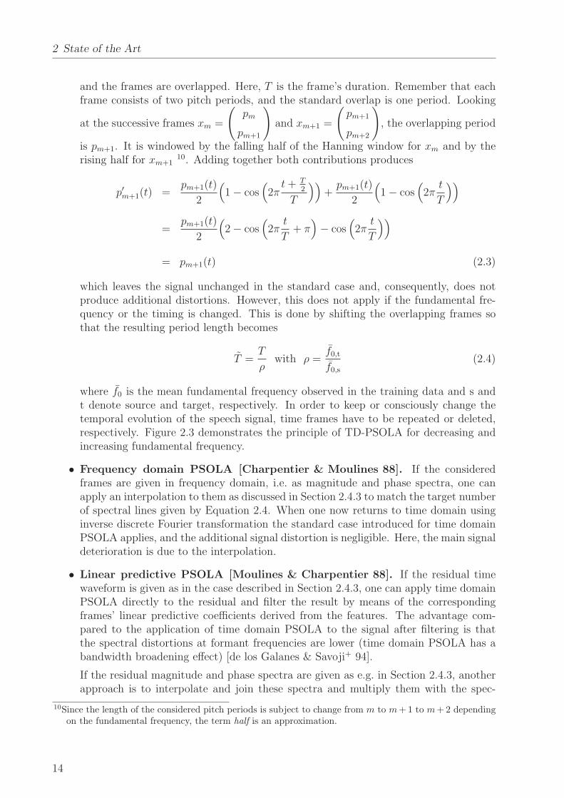
and the frames are overlapped. Here, T is the frame’s duration. Remember that eachframe consists of two pitch periods, and the standard overlap is one period. Looking
at the successive frames xm =
(
pm
pm+1
)
and xm+1 =
(
pm+1
pm+2
)
, the overlapping period
is pm+1. It is windowed by the falling half of the Hanning window for xm and by therising half for xm+1
10. Adding together both contributions produces
p′m+1(t) =pm+1(t)
2
(
1 − cos(
2πt+ T
2
T
))
+pm+1(t)
2
(
1 − cos(
2πt
T
))
=pm+1(t)
2
(
2 − cos(
2πt
T+ π)
− cos(
2πt
T
))
= pm+1(t) (2.3)
which leaves the signal unchanged in the standard case and, consequently, does notproduce additional distortions. However, this does not apply if the fundamental fre-quency or the timing is changed. This is done by shifting the overlapping frames sothat the resulting period length becomes
T =T
ρwith ρ =
f0,t
f0,s
(2.4)
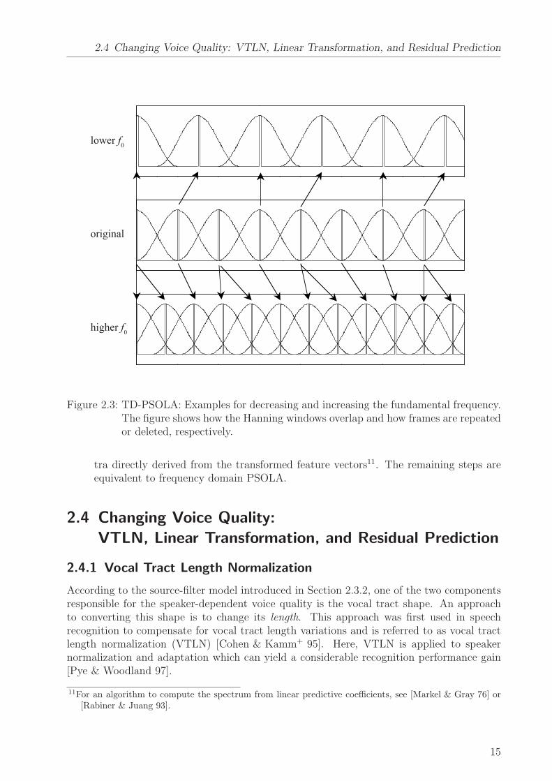
where f0 is the mean fundamental frequency observed in the training data and s andt denote source and target, respectively. In order to keep or consciously change thetemporal evolution of the speech signal, time frames have to be repeated or deleted,respectively. Figure 2.3 demonstrates the principle of TD-PSOLA for decreasing andincreasing fundamental frequency.
• Frequency domain PSOLA [Charpentier & Moulines 88]. If the consideredframes are given in frequency domain, i.e. as magnitude and phase spectra, one canapply an interpolation to them as discussed in Section 2.4.3 to match the target numberof spectral lines given by Equation 2.4. When one now returns to time domain usinginverse discrete Fourier transformation the standard case introduced for time domainPSOLA applies, and the additional signal distortion is negligible. Here, the main signaldeterioration is due to the interpolation.
• Linear predictive PSOLA [Moulines & Charpentier 88]. If the residual timewaveform is given as in the case described in Section 2.4.3, one can apply time domainPSOLA directly to the residual and filter the result by means of the correspondingframes’ linear predictive coefficients derived from the features. The advantage com-pared to the application of time domain PSOLA to the signal after filtering is thatthe spectral distortions at formant frequencies are lower (time domain PSOLA has abandwidth broadening effect) [de los Galanes & Savoji+ 94].
If the residual magnitude and phase spectra are given as e.g. in Section 2.4.3, anotherapproach is to interpolate and join these spectra and multiply them with the spec-
10Since the length of the considered pitch periods is subject to change from m to m + 1 to m + 2 dependingon the fundamental frequency, the term half is an approximation.
14
2.4 Changing Voice Quality: VTLN, Linear Transformation, and Residual Prediction
original
lower f0
higher f0
Figure 2.3: TD-PSOLA: Examples for decreasing and increasing the fundamental frequency.The figure shows how the Hanning windows overlap and how frames are repeatedor deleted, respectively.
tra directly derived from the transformed feature vectors11. The remaining steps areequivalent to frequency domain PSOLA.
2.4 Changing Voice Quality: ...................................
VTLN, Linear Transformation, and Residual Prediction
2.4.1 Vocal Tract Length Normalization
According to the source-filter model introduced in Section 2.3.2, one of the two componentsresponsible for the speaker-dependent voice quality is the vocal tract shape. An approachto converting this shape is to change its length. This approach was first used in speechrecognition to compensate for vocal tract length variations and is referred to as vocal tractlength normalization (VTLN) [Cohen & Kamm+ 95]. Here, VTLN is applied to speakernormalization and adaptation which can yield a considerable recognition performance gain[Pye & Woodland 97].
11For an algorithm to compute the spectrum from linear predictive coefficients, see [Markel & Gray 76] or[Rabiner & Juang 93].
15
2 State of the Art
[Eide & Gish 96] investigated the change of the vocal tract length based on the tubemodel described in Section 2.3.2. They showed that a division of the vocal tract length (thatof the tube sequence) l by a factor α such that l = l
αmeans that the frequency axis of a
sound’s spectrum generated by such a vocal tract is warped reciprocally according to ω = αω.α is usually referred to as warping factor. Consequently, VTLN is performed by applyinga linear warping function to the spectrum of the speech frames. Further investigations intoVTLN have shown that there are more powerful warping functions than the purely linearone. Some of them are discussed in the following.
In speech recognition, only the magnitude spectrum is processed, since the later featur-ization (into mel frequency cepstral coefficients or perceptual linear predictive coefficients[Hermansky 90, Hermansky & Morgan 94]) neglects the phase spectrum which does not seemto be significant for recognition. For its use in voice conversion, however, the phase spectrumalso plays an important role to produce natural speech and, hence, should also be subjectto warping12.
Let 0 ≤ ω ≤ π be the normalized, continuous frequency, then an arbitrary warpingfunction g that depends on a set of parameters {ξ1, ξ2, . . .} is applied to ω yielding the scaledfrequency
ω = g(ω|ξ1, ξ2, . . .) with 0 ≤ ω ≤ π. (2.5)
Accordingly, when a given frame’s (magnitude) spectrum as a function of ω is referred toas X(ω) 13 and the warped counterpart is X then one obtains the following equality takinginto account that the magnitude of the warped spectrum at the warped frequency ω is toequal the source magnitude at the original frequency ω:
X(ω) = X(ω). (2.6)
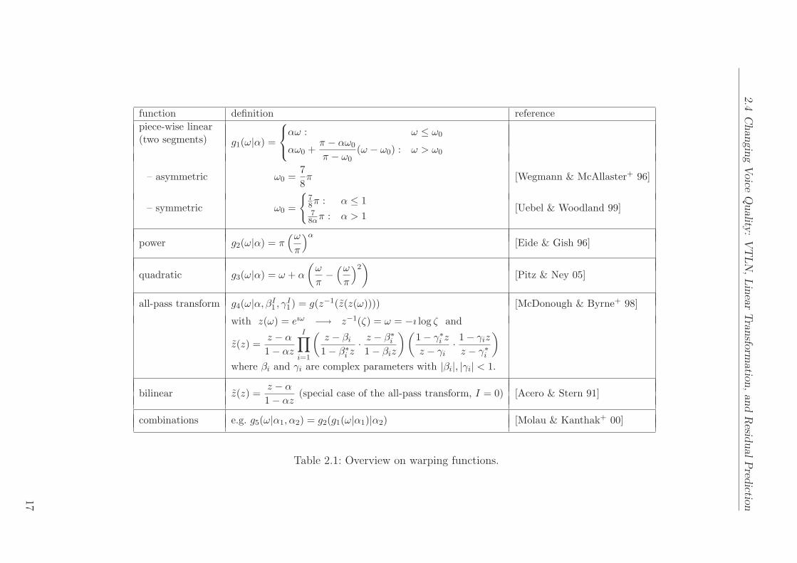
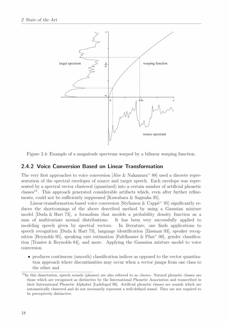
In literature on speech recognition, there is a variety of warping functions, most ofthem based on just one parameter, the warping factor α. Table 2.1 gives an overview oncommonly used functions. Figure 2.4 shows an example frame’s magnitude spectrum warpedby a bilinear warping function.
In speech recognition, the determination of the parameters (mostly the warping factorα), requires the execution of a forced Viterbi alignment on the whole training data involvedfor each parameter candidate [Lee & Rose 96]. The candidate minimizing the score is se-lected.
Referring to candidates suggests that the considered warping factors are taken from adiscrete set, in relevant literature ([Welling & Ney+ 02, Molau 02]) given by14
α ∈ {0.88, 0.9, . . . , 1.12}. (2.7)
Restricting the set to these 13 candidates is supposed to reduce the computational effortfor the parameter estimation and turns out to be a reasonable setting for the use in speechrecognition. In Section 3.1, we will see that when applying VTLN to voice conversion upperand lower limit of the warping factor have to be altered.
12For details on phase interpolation, see Section 2.4.2.13In digital speech processing, we do not have continuous spectra but, due to discrete time sampling and
application of the discrete Fourier transformation, discrete spectra. However, for the current consider-ations and to simplify matters, we assume ω and X(ω) to be continuous. Discrete counterparts of thefollowing derivations can be computed using interpolation methods, e.g. cubic splines [de Boor 78].
14This holds for the piece-wise linear warping function with two segments.
16
2.4
Changin
gV
oice
Quality
:V
TLN
,Lin
ear
Tra
nsfo
rmatio
n,and
Resid
ualP
redictio
n
function definition reference
piece-wise linear(two segments) g1(ω|α) =
αω : ω ≤ ω0
αω0 +π − αω0
π − ω0(ω − ω0) : ω > ω0
– asymmetric ω0 =7
8π [Wegmann & McAllaster+ 96]
– symmetric ω0 =
{
78π : α ≤ 178απ : α > 1
[Uebel & Woodland 99]
power g2(ω|α) = π(ω
π
)α[Eide & Gish 96]
quadratic g3(ω|α) = ω + α
(
ω
π−(ω
π
)2)
[Pitz & Ney 05]
all-pass transform g4(ω|α, βI1 , γI
1) = g(z−1(z(z(ω)))) [McDonough & Byrne+ 98]
with z(ω) = eıω −→ z−1(ζ) = ω = −ı log ζ and
z(z) =z − α
1 − αz
I∏
i=1
(
z − βi
1 − β∗i z
· z − β∗i
1 − βiz
)(
1 − γ∗i z
z − γi· 1 − γiz
z − γ∗i
)
where βi and γi are complex parameters with |βi|, |γi| < 1.
bilinear z(z) =z − α
1 − αz(special case of the all-pass transform, I = 0) [Acero & Stern 91]
combinations e.g. g5(ω|α1, α2) = g2(g1(ω|α1)|α2) [Molau & Kanthak+ 00]
Table 2.1: Overview on warping functions.
17
2 State of the Art
0
0.5π
π
0 0.5π π
source spectrum
target spectrum warping function
Figure 2.4: Example of a magnitude spectrum warped by a bilinear warping function.
2.4.2 Voice Conversion Based on Linear Transformation
The very first approaches to voice conversion [Abe & Nakamura+ 88] used a discrete repre-sentation of the spectral envelopes of source and target speech. Each envelope was repre-sented by a spectral vector clustered (quantized) into a certain number of artificial phoneticclasses15. This approach generated considerable artifacts which, even after further refine-ments, could not be sufficiently suppressed [Kuwabara & Sagisaka 95].
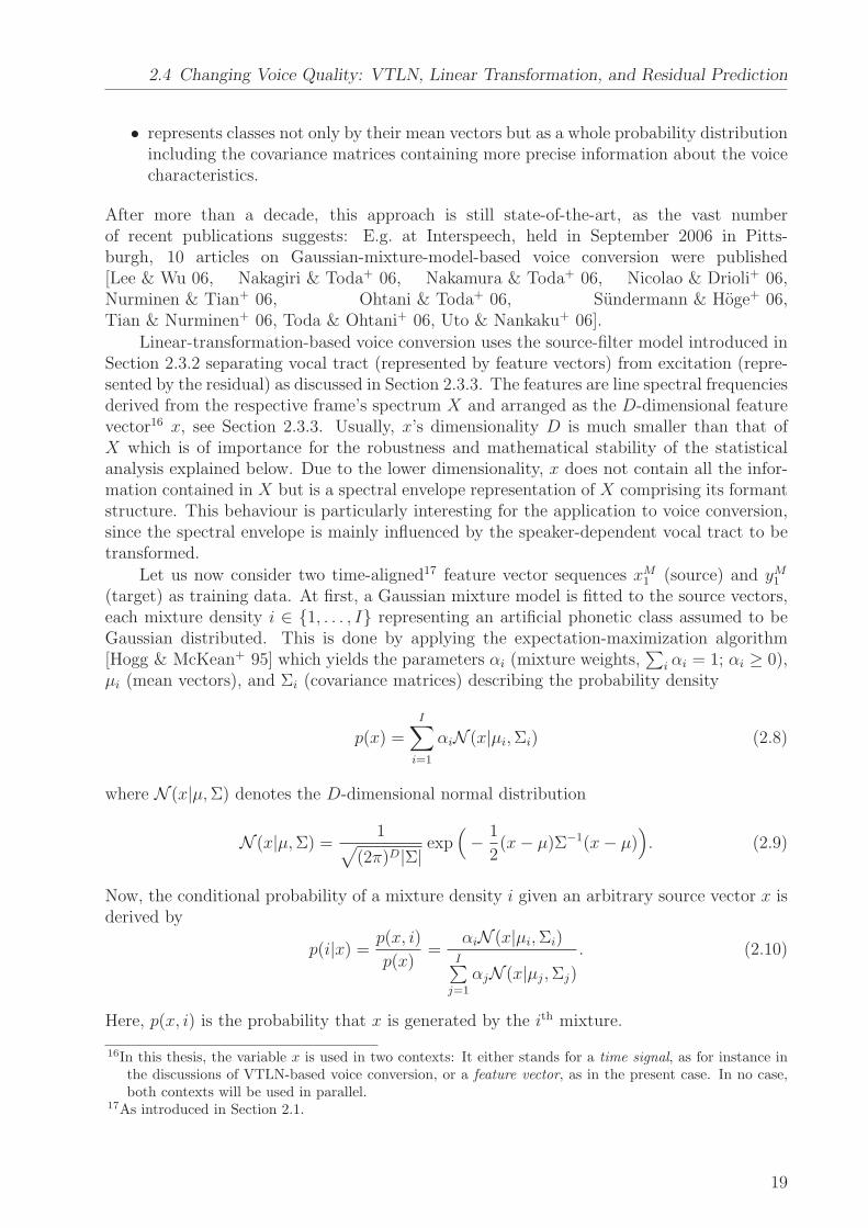
Linear-transformation-based voice conversion [Stylianou & Cappe+ 95] significantly re-duces the shortcomings of the above described method by using a Gaussian mixturemodel [Duda & Hart 73], a formalism that models a probability density function as asum of multivariate normal distributions. It has been very successfully applied tomodeling speech given by spectral vectors. In literature, one finds applications tospeech recognition [Duda & Hart 73], language identification [Zissman 93], speaker recog-nition [Reynolds 95], speaking rate estimation [Faltlhauser & Pfau+ 00], gender classifica-tion [Tranter & Reynolds 04], and more. Applying the Gaussian mixture model to voiceconversion
• produces continuous (smooth) classification indices as opposed to the vector quantiza-tion approach where discontinuities may occur when a vector jumps from one class tothe other and
15In this dissertation, speech sounds (phones) are also referred to as classes. Natural phonetic classes arethose which are recognized as distinctive by the International Phonetic Association and transcribed intheir International Phonetic Alphabet [Ladefoged 90]. Artificial phonetic classes are sounds which areautomatically clustered and do not necessarily represent a well-defined sound. They are not required tobe perceptively distinctive.
18
2.4 Changing Voice Quality: VTLN, Linear Transformation, and Residual Prediction
• represents classes not only by their mean vectors but as a whole probability distributionincluding the covariance matrices containing more precise information about the voicecharacteristics.
After more than a decade, this approach is still state-of-the-art, as the vast numberof recent publications suggests: E.g. at Interspeech, held in September 2006 in Pitts-burgh, 10 articles on Gaussian-mixture-model-based voice conversion were published[Lee & Wu 06, Nakagiri & Toda+ 06, Nakamura & Toda+ 06, Nicolao & Drioli+ 06,Nurminen & Tian+ 06, Ohtani & Toda+ 06, Sundermann & Hoge+ 06,Tian & Nurminen+ 06, Toda & Ohtani+ 06, Uto & Nankaku+ 06].
Linear-transformation-based voice conversion uses the source-filter model introduced inSection 2.3.2 separating vocal tract (represented by feature vectors) from excitation (repre-sented by the residual) as discussed in Section 2.3.3. The features are line spectral frequenciesderived from the respective frame’s spectrum X and arranged as the D-dimensional featurevector16 x, see Section 2.3.3. Usually, x’s dimensionality D is much smaller than that ofX which is of importance for the robustness and mathematical stability of the statisticalanalysis explained below. Due to the lower dimensionality, x does not contain all the infor-mation contained in X but is a spectral envelope representation of X comprising its formantstructure. This behaviour is particularly interesting for the application to voice conversion,since the spectral envelope is mainly influenced by the speaker-dependent vocal tract to betransformed.
Let us now consider two time-aligned17 feature vector sequences xM1 (source) and yM
1
(target) as training data. At first, a Gaussian mixture model is fitted to the source vectors,each mixture density i ∈ {1, . . . , I} representing an artificial phonetic class assumed to beGaussian distributed. This is done by applying the expectation-maximization algorithm[Hogg & McKean+ 95] which yields the parameters αi (mixture weights,
∑
i αi = 1; αi ≥ 0),µi (mean vectors), and Σi (covariance matrices) describing the probability density
p(x) =I∑
i=1
αiN (x|µi,Σi) (2.8)
where N (x|µ,Σ) denotes the D-dimensional normal distribution
N (x|µ,Σ) =1
√
(2π)D|Σ|exp
(
− 1
2(x− µ)Σ−1(x− µ)
)
. (2.9)
Now, the conditional probability of a mixture density i given an arbitrary source vector x isderived by
p(i|x) =p(x, i)
p(x)=
αiN (x|µi,Σi)I∑
j=1
αjN (x|µj,Σj)
. (2.10)
Here, p(x, i) is the probability that x is generated by the ith mixture.
16In this thesis, the variable x is used in two contexts: It either stands for a time signal, as for instance inthe discussions of VTLN-based voice conversion, or a feature vector, as in the present case. In no case,both contexts will be used in parallel.
17As introduced in Section 2.1.
19
2 State of the Art
The voice transformation function F that converts a given source vector x to a vectorx supposed to represent spectral contents similar to the target voice is expressed by a lineartransformation
x = F (x) = Ax+ b (2.11)
or, considering mixture-dependent transformations18,
F (x) = F (x|AI1, b
I1) =
I∑
i=1
p(i|x)(Aix+ bi). (2.12)
Finally, the unknown parameters Ai, matrices of size D×D, and bi, vectors of dimensionalityD are to be estimated based on the least squares technique where the sum of the squareddistances between the transformed vectors xm = F (xm|AI
1, bI1) and the aligned target vectors
ym for m ∈ {1, . . . ,M} is minimized19:
M∑
m=1
|ym − F (xm|AI1, b
I1)|2 = min! (2.13)
In [Stylianou & Cappe+ 98], a solution to this least square problem is carried out showingthat AI
1 and bI1 can be expressed as a linear combination of αI1, µ
I1, and ΣI
1.In conversion phase, a new source speaker utterance is featurized, the resulting feature
vector sequence is converted using the voice transformation function F . Section 2.4.3 isdedicated to how to transform the resulting feature vectors to time domain.
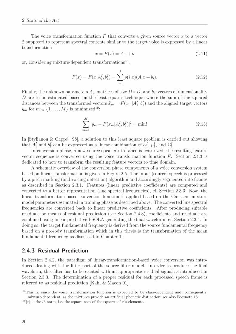
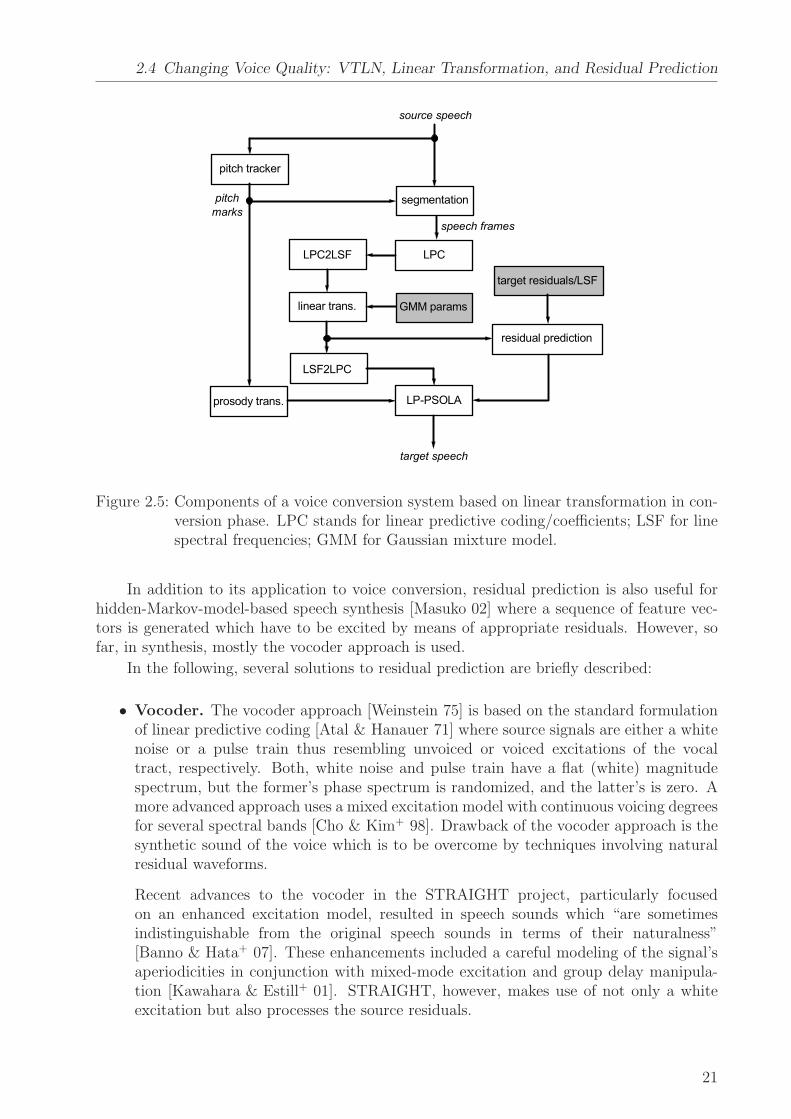
A schematic overview of the conversion phase components of a voice conversion systembased on linear transformation is given in Figure 2.5. The input (source) speech is processedby a pitch marking (and voicing detection) algorithm and accordingly segmented into framesas described in Section 2.3.1. Features (linear predictive coefficients) are computed andconverted to a better representation (line spectral frequencies), cf. Section 2.3.3. Now, thelinear-transformation-based conversion function is applied based on the Gaussian mixturemodel parameters estimated in training phase as described above. The converted line spectralfrequencies are converted back to linear predictive coefficients. After producing suitableresiduals by means of residual prediction (see Section 2.4.3), coefficients and residuals arecombined using linear predictive PSOLA generating the final waveform, cf. Section 2.3.4. Indoing so, the target fundamental frequency is derived from the source fundamental frequencybased on a prosody transformation which in this thesis is the transformation of the meanfundamental frequency as discussed in Chapter 1.
2.4.3 Residual Prediction
In Section 2.4.2, the paradigm of linear-transformation-based voice conversion was intro-duced dealing with the filter part of the source-filter model. In order to produce the finalwaveform, this filter has to be excited with an appropriate residual signal as introduced inSection 2.3.3. The determination of a proper residual for each processed speech frame isreferred to as residual prediction [Kain & Macon 01].
18This is, since the voice transformation function is expected to be class-dependent and, consequently,mixture-dependent, as the mixtures provide an artificial phonetic distinction; see also Footnote 15.
19|x| is the l2-norm, i.e. the square root of the squares of x’s elements.
20
2.4 Changing Voice Quality: VTLN, Linear Transformation, and Residual Prediction
Figure 2.5: Components of a voice conversion system based on linear transformation in con-version phase. LPC stands for linear predictive coding/coefficients; LSF for linespectral frequencies; GMM for Gaussian mixture model.
In addition to its application to voice conversion, residual prediction is also useful forhidden-Markov-model-based speech synthesis [Masuko 02] where a sequence of feature vec-tors is generated which have to be excited by means of appropriate residuals. However, sofar, in synthesis, mostly the vocoder approach is used.
In the following, several solutions to residual prediction are briefly described:
• Vocoder. The vocoder approach [Weinstein 75] is based on the standard formulationof linear predictive coding [Atal & Hanauer 71] where source signals are either a whitenoise or a pulse train thus resembling unvoiced or voiced excitations of the vocaltract, respectively. Both, white noise and pulse train have a flat (white) magnitudespectrum, but the former’s phase spectrum is randomized, and the latter’s is zero. Amore advanced approach uses a mixed excitation model with continuous voicing degreesfor several spectral bands [Cho & Kim+ 98]. Drawback of the vocoder approach is thesynthetic sound of the voice which is to be overcome by techniques involving naturalresidual waveforms.
Recent advances to the vocoder in the STRAIGHT project, particularly focusedon an enhanced excitation model, resulted in speech sounds which “are sometimesindistinguishable from the original speech sounds in terms of their naturalness”[Banno & Hata+ 07]. These enhancements included a careful modeling of the signal’saperiodicities in conjunction with mixed-mode excitation and group delay manipula-tion [Kawahara & Estill+ 01]. STRAIGHT, however, makes use of not only a whiteexcitation but also processes the source residuals.
21
2 State of the Art
• Copying source residuals. When considering residual prediction for its applicationto voice conversion we are given natural speech as input whose time-alignment to theoutput speech is well known. Hence, for every output frame, at least the correspondinginput residual is known. According to the ideal source-filter model, one might expectmost of the speaker-dependent information to be represented by the vocal tract and,consequently, by the features. The excitation and, consequently, the residuals, might beexpected to be less crucial for the voice characteristics, thus, finally, a simple solutionwould be to directly use the source as target residuals and apply the transformedfeatures. This technique was used by [Kain & Macon 98], but they stated that “merelychanging the [spectral envelope] is not sufficient for changing the speaker identity”.Most of the listeners “had the impression that a ‘third’ speaker was created”.
• Residual codebook method. In addition to the observation that the residual signalalso contains speaker-dependent information, it turns out that spectral features andcorresponding residuals are correlated [Kain 01]. This insight led to the idea that theresiduals of the converted speech could be predicted based on the converted featurevectors and resulted in the following residual prediction technique.
In training phase, similar to Section 2.4.2, the probability distribution of the targetfeature vectors yM
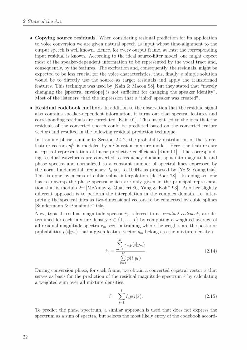
1 is modeled by a Gaussian mixture model. Here, the features area cepstral representation of linear predictive coefficients [Kain 01]. The correspond-ing residual waveforms are converted to frequency domain, split into magnitude andphase spectra and normalized to a constant number of spectral lines expressed bythe norm fundamental frequency fn set to 100Hz as proposed by [Ye & Young 04a].This is done by means of cubic spline interpolation [de Boor 78]. In doing so, onehas to unwrap the phase spectra which are only given in the principal representa-tion that is modulo 2π [McAulay & Quatieri 86, Yang & Koh+ 93]. Another slightlydifferent approach is to perform the interpolation in the complex domain, i.e. inter-preting the spectral lines as two-dimensional vectors to be connected by cubic splines[Sundermann & Bonafonte+ 04a].
Now, typical residual magnitude spectra ri, referred to as residual codebook, are de-termined for each mixture density i ∈ {1, . . . , I} by computing a weighted average ofall residual magnitude spectra rm seen in training where the weights are the posteriorprobabilities p(i|ym) that a given feature vector ym belongs to the mixture density i:
ri =
M∑
m=1
rmp(i|ym)
M∑
k=1
p(i|yk)
. (2.14)
During conversion phase, for each frame, we obtain a converted cepstral vector x thatserves as basis for the prediction of the residual magnitude spectrum r by calculatinga weighted sum over all mixture densities:
r =I∑
i=1
rip(i|x). (2.15)
To predict the phase spectrum, a similar approach is used that does not express thespectrum as a sum of spectra, but selects the most likely entry of the codebook accord-
22
2.5 Evaluation Metrics for Voice Conversion
ing to the posterior probability p(i|x) and finally applies a smoothing to avoid phasediscontinuities.
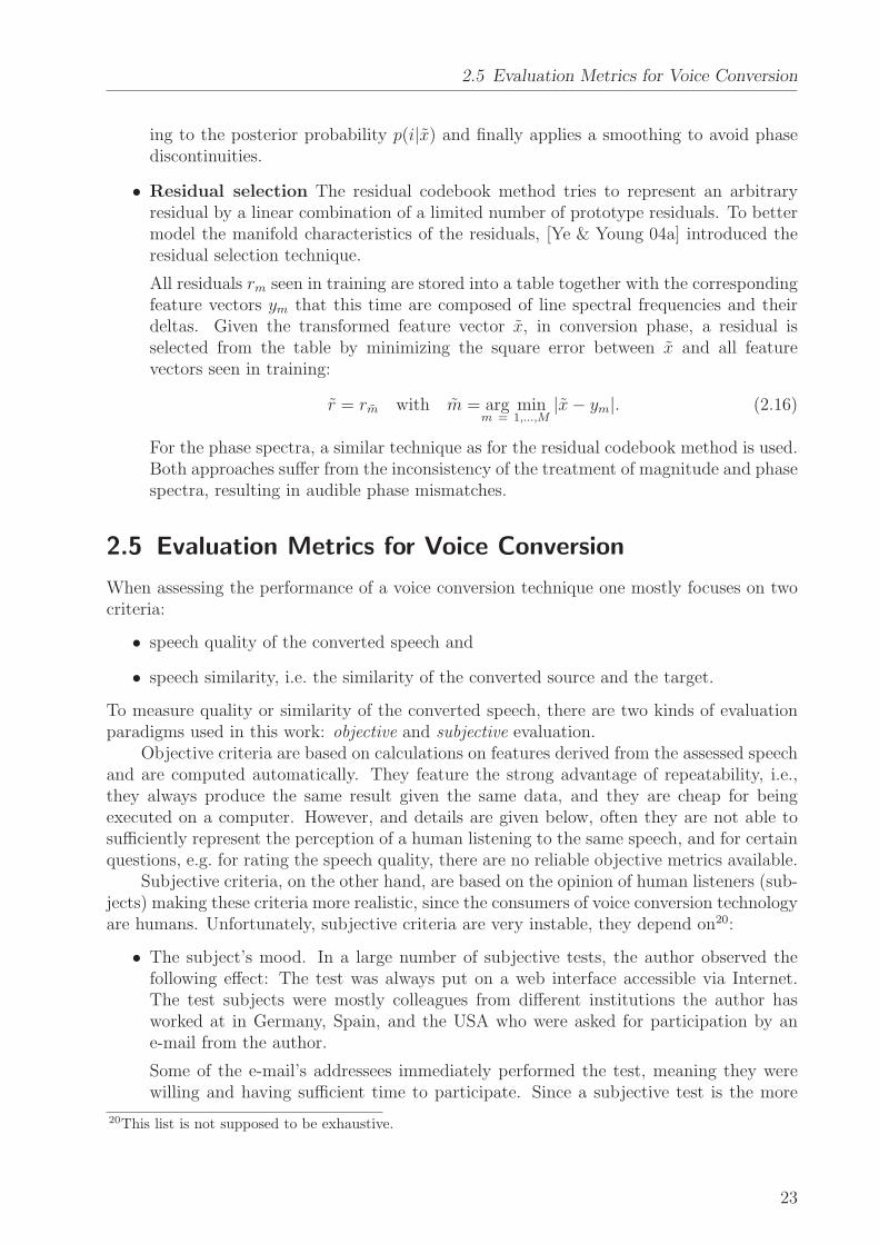
• Residual selection The residual codebook method tries to represent an arbitraryresidual by a linear combination of a limited number of prototype residuals. To bettermodel the manifold characteristics of the residuals, [Ye & Young 04a] introduced theresidual selection technique.
All residuals rm seen in training are stored into a table together with the correspondingfeature vectors ym that this time are composed of line spectral frequencies and theirdeltas. Given the transformed feature vector x, in conversion phase, a residual isselected from the table by minimizing the square error between x and all featurevectors seen in training:
r = rm with m = arg minm = 1,...,M
|x− ym|. (2.16)
For the phase spectra, a similar technique as for the residual codebook method is used.Both approaches suffer from the inconsistency of the treatment of magnitude and phasespectra, resulting in audible phase mismatches.
2.5 Evaluation Metrics for Voice Conversion
When assessing the performance of a voice conversion technique one mostly focuses on twocriteria:
• speech quality of the converted speech and
• speech similarity, i.e. the similarity of the converted source and the target.
To measure quality or similarity of the converted speech, there are two kinds of evaluationparadigms used in this work: objective and subjective evaluation.
Objective criteria are based on calculations on features derived from the assessed speechand are computed automatically. They feature the strong advantage of repeatability, i.e.,they always produce the same result given the same data, and they are cheap for beingexecuted on a computer. However, and details are given below, often they are not able tosufficiently represent the perception of a human listening to the same speech, and for certainquestions, e.g. for rating the speech quality, there are no reliable objective metrics available.
Subjective criteria, on the other hand, are based on the opinion of human listeners (sub-jects) making these criteria more realistic, since the consumers of voice conversion technologyare humans. Unfortunately, subjective criteria are very instable, they depend on20:
• The subject’s mood. In a large number of subjective tests, the author observed thefollowing effect: The test was always put on a web interface accessible via Internet.The test subjects were mostly colleagues from different institutions the author hasworked at in Germany, Spain, and the USA who were asked for participation by ane-mail from the author.
Some of the e-mail’s addressees immediately performed the test, meaning they werewilling and having sufficient time to participate. Since a subjective test is the more
20This list is not supposed to be exhaustive.
23
2 State of the Art
16 18 20 22 24 26 28 30
2.5
2.6
2.7
2.8
MOS Q
# subjects
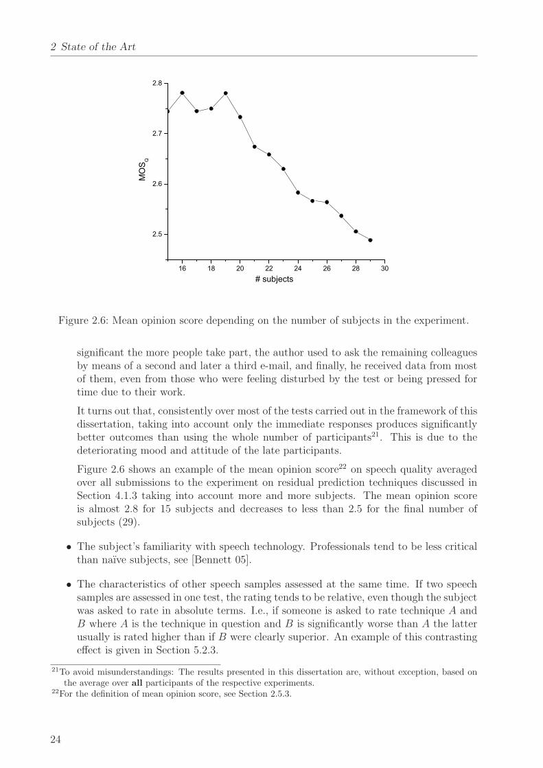
Figure 2.6: Mean opinion score depending on the number of subjects in the experiment.
significant the more people take part, the author used to ask the remaining colleaguesby means of a second and later a third e-mail, and finally, he received data from mostof them, even from those who were feeling disturbed by the test or being pressed fortime due to their work.
It turns out that, consistently over most of the tests carried out in the framework of thisdissertation, taking into account only the immediate responses produces significantlybetter outcomes than using the whole number of participants21. This is due to thedeteriorating mood and attitude of the late participants.
Figure 2.6 shows an example of the mean opinion score22 on speech quality averagedover all submissions to the experiment on residual prediction techniques discussed inSection 4.1.3 taking into account more and more subjects. The mean opinion scoreis almost 2.8 for 15 subjects and decreases to less than 2.5 for the final number ofsubjects (29).
• The subject’s familiarity with speech technology. Professionals tend to be less criticalthan naıve subjects, see [Bennett 05].
• The characteristics of other speech samples assessed at the same time. If two speechsamples are assessed in one test, the rating tends to be relative, even though the subjectwas asked to rate in absolute terms. I.e., if someone is asked to rate technique A andB where A is the technique in question and B is significantly worse than A the latterusually is rated higher than if B were clearly superior. An example of this contrastingeffect is given in Section 5.2.3.
21To avoid misunderstandings: The results presented in this dissertation are, without exception, based onthe average over all participants of the respective experiments.
22For the definition of mean opinion score, see Section 2.5.3.
24
2.5 Evaluation Metrics for Voice Conversion
quality similarity
objective – log-spectral distortion
subjective mean opinion score extended ABX,mean opinion score
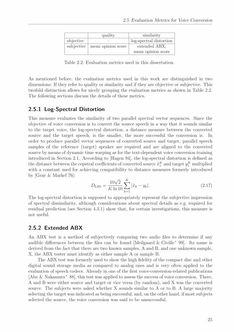
Table 2.2: Evaluation metrics used in this dissertation.
As mentioned before, the evaluation metrics used in this work are distinguished in twodimensions: If they refer to quality or similarity and if they are objective or subjective. Thistwofold distinction allows for nicely grouping the evaluation metrics as shown in Table 2.2.The following sections discuss the details of these metrics.
2.5.1 Log-Spectral Distortion
This measure evaluates the similarity of two parallel spectral vector sequences. Since theobjective of voice conversion is to convert the source speech in a way that it sounds similarto the target voice, the log-spectral distortion, a distance measure between the convertedsource and the target speech, is the smaller, the more successful the conversion is. Inorder to produce parallel vector sequences of converted source and target, parallel speechsamples of the reference (target) speaker are required and are aligned to the convertedsource by means of dynamic time warping as for the text-dependent voice conversion trainingintroduced in Section 2.1. According to [Hagen 94], the log-spectral distortion is defined asthe distance between the cepstral coefficients of converted source xK
1 and target yK1 multiplied
with a constant used for achieving compatibility to distance measures formerly introducedby [Gray & Markel 76]:
DLSD =10√
2
K ln 10
K∑
k=1
|xk − yk|. (2.17)
The log-spectral distortion is supposed to appropriately represent the subjective impressionof spectral dissimilarity, although considerations about spectral details as e.g. required forresidual prediction (see Section 4.3.1) show that, for certain investigations, this measure isnot useful.
2.5.2 Extended ABX
An ABX test is a method of subjectively comparing two audio files to determine if anyaudible differences between the files can be found [Meilgaard & Civille+ 99]. Its name isderived from the fact that there are two known samples, A and B, and one unknown sample,X, the ABX tester must identify as either sample A or sample B.
The ABX test was formerly used to show the high fidelity of the compact disc and otherdigital sound storage media as compared to analog ones and is very often applied to theevaluation of speech codecs. Already in one of the first voice-conversion-related publications[Abe & Nakamura+ 88], this test was applied to assess the success of voice conversion. There,A and B were either source and target or vice versa (by random), and X was the convertedsource. The subjects were asked whether X sounds similar to A or to B. A large majorityselecting the target was indicated as being successful, and, on the other hand, if most subjectsselected the source, the voice conversion was said to be unsuccessful.
25
2 State of the Art
MOS quality similarity
5 excellent identical4 good similar3 fair uncertain2 poor dissimilar1 bad different
Table 2.3: Mean opinion score rating scheme.
This paradigm was used over a decade until [Kain & Macon 98] observed that severalof their experiments showed an almost uniformal distribution among source and target voicewhich could have been interpreted as being fairly successful. However, when interview-ing the subjects they found “that many had the impression that a third [...] speaker wascreated” and, therefore, tended to decide by chance. In order to identify this category,this dissertation’s author introduced a third choice to the test and called it extended ABX[Sundermann & Bonafonte+ 04b]. Here, the subject is asked whether voice X sounded like
(1) voice A,
(2) voice B, or
(3) neither of them.
2.5.3 Mean Opinion Score
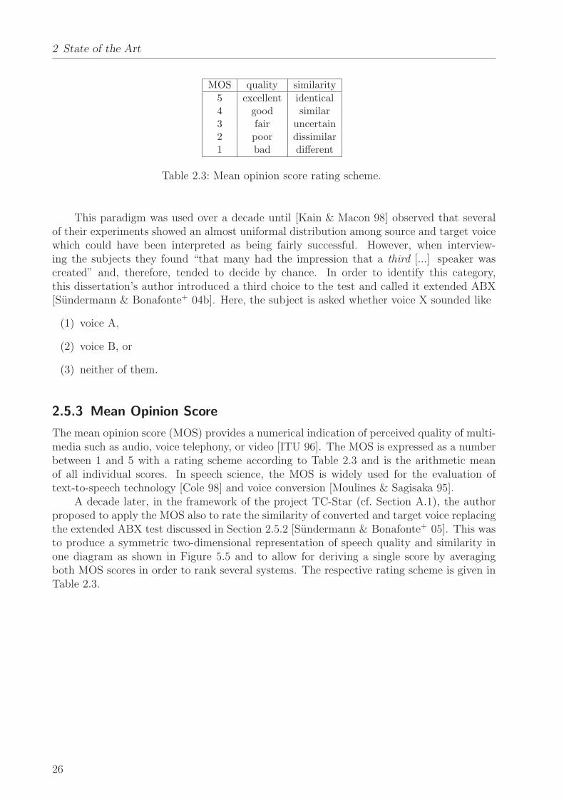
The mean opinion score (MOS) provides a numerical indication of perceived quality of multi-media such as audio, voice telephony, or video [ITU 96]. The MOS is expressed as a numberbetween 1 and 5 with a rating scheme according to Table 2.3 and is the arithmetic meanof all individual scores. In speech science, the MOS is widely used for the evaluation oftext-to-speech technology [Cole 98] and voice conversion [Moulines & Sagisaka 95].
A decade later, in the framework of the project TC-Star (cf. Section A.1), the authorproposed to apply the MOS also to rate the similarity of converted and target voice replacingthe extended ABX test discussed in Section 2.5.2 [Sundermann & Bonafonte+ 05]. This wasto produce a symmetric two-dimensional representation of speech quality and similarity inone diagram as shown in Figure 5.5 and to allow for deriving a single score by averagingboth MOS scores in order to rank several systems. The respective rating scheme is given inTable 2.3.
26
3 VTLN-Based Voice Conversion
The considerable performance gain achieved when applying VTLN to speech recognitionmentioned in Section 2.4.1 suggested that the proposed frequency warping changed an im-portant part of the voice characteristics towards a given target (the norm voice). Since afterwarping, the spectra can be easily transformed back to an audible time signal by means offrequency domain PSOLA (see Section 2.3.4), its use for voice conversion seems promising.
3.1 Parameter Training
In Section 2.4.1, it was mentioned that the parameters of the considered warping functionsare determined by performing a forced alignment on the whole training data for each pa-rameter candidate and searching for the parameter resulting in the maximum score. Sincein the case of voice conversion, we are given parallel speech of source and target (cf. Sec-tion 2.1), the optimal parameter candidate can be estimated by comparing converted sourceand target speech frame by frame, accumulating the distances between corresponding framesand choosing the candidate with the lowest result. In doing so, voiced frames are to be pre-ferred, as, generally, they contain much more vocal-tract-related information than unvoicedframes23. Consequently the accumulation of the aforementioned distances is performed byweighting the respective frames’ contributions by their voicing degree vm as introduced inSection 2.3.4:
ξI1 = arg min
ξ′I′1
M∑
m=1
vm|Ym − Xm(ξ′I′1)|2 (3.1)
where |X| is the continuous equivalent to the definition of the l2-norm according to Foot-note 19:
|X| =
√
1
π
∫ π
0
|X(ω)|2 dω. (3.2)
Compared to the very time-consuming estimation of the warping factor in speech recognition,this procedure is rather fast, particularly when taking into account that the amount of speechconsidered in the voice conversion task rarely exceeds 15 minutes (cf. corpora descriptions inSection A.2), whereas in speech recognition, sometimes databases of several thousand hoursof speech are employed [Evermann & Chan+ 05]. At least this holds when the search spaceis kept as limited as mentioned earlier for applications to speech recognition in Equation 2.7:
ξ′I′1 = α′ ∈ {0.88, 0.9, . . . , 1.12}. (3.3)
For two reasons, however, the search space has to be enlarged when being applied to voiceconversion:
23[Ye & Young 04a] observed that “unvoiced sounds contain very little vocal tract information [...]. Hence,in common with other [voice conversion] systems, unvoiced frames [...] are simply copied to the target.”
3 VTLN-Based Voice Conversion
• According to the definition of VTLN (see Section 2.4.1), this technique aims at compen-sating for variations in the vocal tract length and normalizing it to a norm value whichis located symmetrically between the extrema α = 0.88 and α = 1.12. When appliedto voice conversion the objective is slightly different. Here, one aims at transformingthe vocal tract length from a given voice to an arbitrary other voice. If the sourcevoice is already an extreme voice (e.g. a child featuring a very short vocal tract), andthe target voice is the other extremum (a bass voice with large vocal tract), the rangeof warping is about double of that expected in the normalization case of speech recog-nition24. Consequently, for the piece-wise linear warping function with two segments,the final range would be
α′ ∈ {0.76, 0.78, . . . , 1.24}. (3.4)
• In Table 2.1, two warping functions depending on several parameters were introduced.They give more flexibility for changing the voice characteristics in the voice conversionframework on the one hand, but raise the problem of how to estimate these parameterson the other hand.
For the case of combining k warping functions with one parameter each (see last rowof Table 2.1) whose cardinality25 is c, one obtains ck different combinations of warpingfactors to be searched. This search is only tractable if k is small.
In the case of the all-pass transform and given a considerable number of parameters,the estimation using a full search is not tractable anymore. [Sundermann & Ney+ 03b]presented a parameter estimation algorithm based on the gradient descend method[Avriel 76]. Since this method delivers a local optimum in the neighborhood of a giveninitial parameter setting, a large number of Gaussian distributed initial parametersettings were applied in order to find the global optimum.
3.2 A Piece-Wise Linear Warping Function with Several
Segments
The variety of mostly non-linear warping functions featuring different parameter ranges andcharacteristics as well as the computational effort to estimate the warping parameters calls fora generalized warping function with several parameters that can be computed fast and easily.For that purpose, the author defines a function composed of I + 1 linear segments fulfillingthe following constraints common with the conventional warping functions of Table 2.1:
• The function is continuous.
• The function is monotonous.
• The function is bounded in domain as well as in co-domain to values between 0 and πalso serving as starting and ending points.
24This suggests that the term vocal tract length normalization is not completely adequate to its applicationto voice conversion. Words like adaptation, transformation, or conversion seem to better represent thedescribed technique. However, for the considerable popularity of the acronym VTLN in the speechcommunity, the author decided to ignore this slight imprecision.
25The number of members of the set of parameters. E.g., the cardinality of the set of all possible α′ inEquation 3.4 is 25.
28
3.2 A Piece-Wise Linear Warping Function with Several Segments
0.0 0.2 0.4 0.6 0.8 1.00.0
0.2
0.4
0.6
0.8
1.0
ωπ
. ωπ
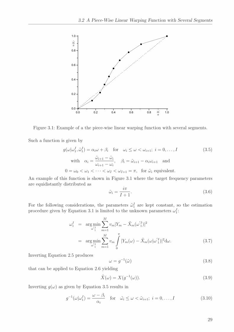
Figure 3.1: Example of a the piece-wise linear warping function with several segments.
Such a function is given by
g(ω|ωI1 , ω
I1) = αiω + βi for ωi ≤ ω < ωi+1; i = 0, . . . , I (3.5)
with αi =ωi+1 − ωi
ωi+1 − ωi
, βi = ωi+1 − αiωi+1 and
0 = ω0 < ω1 < · · · < ωI < ωI+1 = π, for ωi equivalent.
An example of this function is shown in Figure 3.1 where the target frequency parametersare equidistantly distributed as
ωi =iπ
I + 1. (3.6)
For the following considerations, the parameters ωI1 are kept constant, so the estimation
procedure given by Equation 3.1 is limited to the unknown parameters ωI1 :
ωI1 = arg min
ω′I′1
M∑
m=1
vm|Ym − Xm(ω′I′1)|2
= arg minω′I′1
M∑
m=1
vm
π∫
0
|Ym(ω) − Xm(ω|ω′I′1)|2dω. (3.7)
Inverting Equation 2.5 producesω = g−1(ω) (3.8)
that can be applied to Equation 2.6 yielding
X(ω) = X(g−1(ω)). (3.9)
Inverting g(ω) as given by Equation 3.5 results in
g−1(ω|ωI1) =
ω − βi
αi
for ωi ≤ ω < ωi+1; i = 0, . . . , I (3.10)
29
3 VTLN-Based Voice Conversion
which is inserted into Equation 3.9:
X(ω|ωI1) = X
(
ω − βi
αi
)
for ωi ≤ ω < ωi+1; i = 0, . . . , I. (3.11)
This allows for breaking the integral of Equation 3.7 down into a sum of partial integrals:
ωI1 = arg min
ω′I′1
M∑
m=1
vm
I∑
i=0
ωi+1∫
ωi
∣
∣
∣Ym(ω) −Xm
(ω − βi
αi
|ω′I′1
)∣
∣
∣
2
dω. (3.12)
Exploiting the fact that αi and βi only depend on the unknown variables ωi and ωi+1 yields
ωI1 = arg min
ω′I′1
I∑
i=0
M∑
m=1
vm
ωi+1∫
ωi
∣
∣
∣Ym(ω) −Xm
(ω − βi
αi
|ω′i, ω
′i+1
)∣
∣
∣
2
dω
= arg minω′I′1
I∑
i=0
G(ω′i, ω
′i+1). (3.13)
Now, the auxiliary quantity Q is introduced as
Q(i, ν) = minνi1;
νi=ν
i∑
j=1
G(νj−1, νj)
= minνi
i−1
[
G(νi−1, νi) + minν′i−1′1
;
ν′i−1=νi−1
i−1∑
j=1
G(νj−1, νj)
]
= minνi
i−1
[
G(νi−1, νi) +Q(i− 1, νi−1)]
. (3.14)
Inserting this recursion formula into Equation 3.13 and setting the initial quantityQ(0, 0) = 0produces
ωI1 = argQ(I + 1, π). (3.15)
This shows that the problem can be broken down into simpler subproblems that require aminimization of two rather than I parameters, i.e., it is a typical dynamic programmingproblem [Cormen & Leiserson+ 90]. The complexity of a straightforward search over allparameter combinations of ω
′I′1 is O(cI), whereas solving the subproblems corresponds to
only O(Ic2). For c cf. Footnote 25.
3.3 Frequency Domain vs. Time Domain VTLN
So far, this chapter’s considerations dealt with parameter estimation of VTLN-based voiceconversion that takes place in the training phase. Often, the training can be performedoffline so that there are no strong restrictions with respect to real-time ability and memory
30
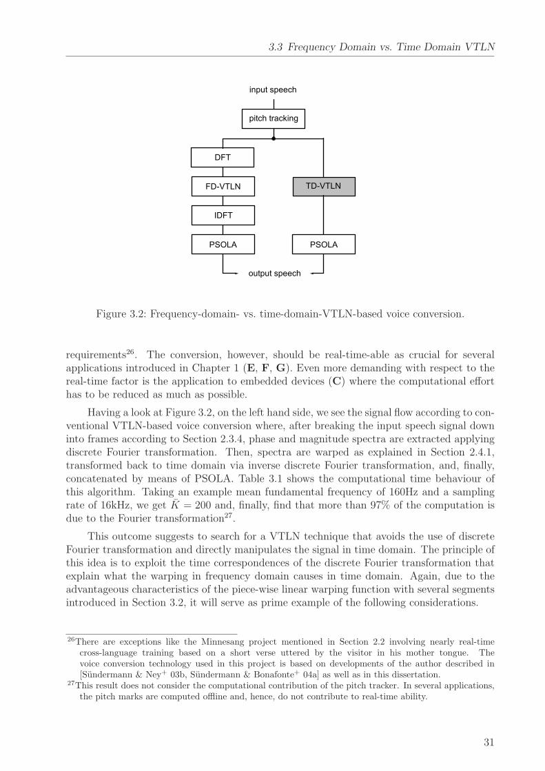
3.3 Frequency Domain vs. Time Domain VTLN
.................
TD-VTLN
input speech
output speech
PSOLAPSOLA
IDFT
FD-VTLN
DFT
pitch tracking
Figure 3.2: Frequency-domain- vs. time-domain-VTLN-based voice conversion.
requirements26. The conversion, however, should be real-time-able as crucial for severalapplications introduced in Chapter 1 (E, F, G). Even more demanding with respect to thereal-time factor is the application to embedded devices (C) where the computational efforthas to be reduced as much as possible.
Having a look at Figure 3.2, on the left hand side, we see the signal flow according to con-ventional VTLN-based voice conversion where, after breaking the input speech signal downinto frames according to Section 2.3.4, phase and magnitude spectra are extracted applyingdiscrete Fourier transformation. Then, spectra are warped as explained in Section 2.4.1,transformed back to time domain via inverse discrete Fourier transformation, and, finally,concatenated by means of PSOLA. Table 3.1 shows the computational time behaviour ofthis algorithm. Taking an example mean fundamental frequency of 160Hz and a samplingrate of 16kHz, we get K = 200 and, finally, find that more than 97% of the computation isdue to the Fourier transformation27.
This outcome suggests to search for a VTLN technique that avoids the use of discreteFourier transformation and directly manipulates the signal in time domain. The principle ofthis idea is to exploit the time correspondences of the discrete Fourier transformation thatexplain what the warping in frequency domain causes in time domain. Again, due to theadvantageous characteristics of the piece-wise linear warping function with several segmentsintroduced in Section 3.2, it will serve as prime example of the following considerations.
26There are exceptions like the Minnesang project mentioned in Section 2.2 involving nearly real-timecross-language training based on a short verse uttered by the visitor in his mother tongue. Thevoice conversion technology used in this project is based on developments of the author described in[Sundermann & Ney+ 03b, Sundermann & Bonafonte+ 04a] as well as in this dissertation.
27This result does not consider the computational contribution of the pitch tracker. In several applications,the pitch marks are computed offline and, hence, do not contribute to real-time ability.
31
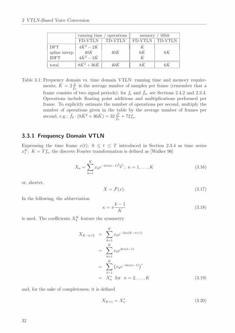
3 VTLN-Based Voice Conversion
running time / operations memory / 16bitFD-VTLN TD-VTLN FD-VTLN TD-VTLN
DFT 4K2 − 2K K
spline interp. 40K 40K 6K 6K
IDFT 4K2 − 2K K
total 8K2 + 36K 40K 8K 6K
Table 3.1: Frequency domain vs. time domain VTLN: running time and memory require-ments; K = 2 fs
¯f0is the average number of samples per frame (remember that a
frame consists of two signal periods); for fs and f0, see Sections 2.4.2 and 2.3.4.Operations include floating point additions and multiplications performed perframe. To explicitly estimate the number of operations per second, multiply thenumber of operations given in the table by the average number of frames per
second, e.g.: f0 · (8K2 + 36K) = 32 f2s
¯f0+ 72fs.
3.3.1 Frequency Domain VTLN
Expressing the time frame x(t); 0 ≤ t ≤ T introduced in Section 2.3.4 as time seriesxK
1 ; K = Tfs, the discrete Fourier transformation is defined as [Walker 96]
Xn =K∑
k=1
xke−2πı(n−1) k−1
K ; n = 1, . . . , K (3.16)
or, shorter,
X = F(x). (3.17)
In the following, the abbreviation
κ = πk − 1
K(3.18)
is used. The coefficients XK2 feature the symmetry
XK−n+2 =K∑
k=1
xke−2κı(K−n+1)
=K∑
k=1
xke2κı(n−1)
=K∑
k=1
(
xke−2κı(n−1)
)∗
= X∗n for n = 2, . . . , K (3.19)
and, for the sake of completeness, it is defined
XK+1 = X∗1 . (3.20)
32
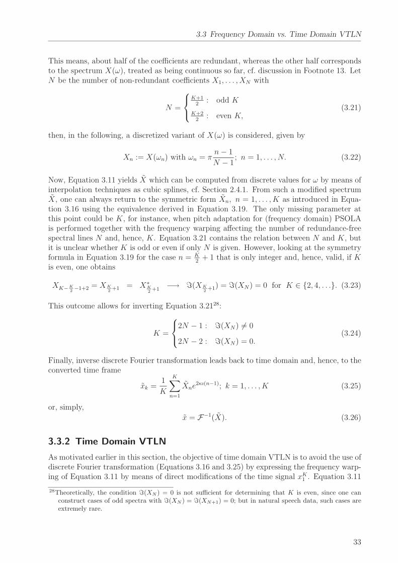
3.3 Frequency Domain vs. Time Domain VTLN
This means, about half of the coefficients are redundant, whereas the other half correspondsto the spectrum X(ω), treated as being continuous so far, cf. discussion in Footnote 13. LetN be the number of non-redundant coefficients X1, . . . , XN with
N =
K+12
: odd K
K+22
: even K,(3.21)
then, in the following, a discretized variant of X(ω) is considered, given by
Xn := X(ωn) with ωn = πn− 1
N − 1; n = 1, . . . , N. (3.22)
Now, Equation 3.11 yields X which can be computed from discrete values for ω by means ofinterpolation techniques as cubic splines, cf. Section 2.4.1. From such a modified spectrumX, one can always return to the symmetric form Xn, n = 1, . . . , K as introduced in Equa-tion 3.16 using the equivalence derived in Equation 3.19. The only missing parameter atthis point could be K, for instance, when pitch adaptation for (frequency domain) PSOLAis performed together with the frequency warping affecting the number of redundance-freespectral lines N and, hence, K. Equation 3.21 contains the relation between N and K, butit is unclear whether K is odd or even if only N is given. However, looking at the symmetryformula in Equation 3.19 for the case n = K
2+ 1 that is only integer and, hence, valid, if K
is even, one obtains
XK−K2−1+2 = XK
2+1 = X∗
K2
+1−→ ℑ(XK
2+1) = ℑ(XN) = 0 for K ∈ {2, 4, . . .}. (3.23)
This outcome allows for inverting Equation 3.2128:
K =
2N − 1 : ℑ(XN) 6= 0
2N − 2 : ℑ(XN) = 0.(3.24)
Finally, inverse discrete Fourier transformation leads back to time domain and, hence, to theconverted time frame
xk =1
K
K∑
n=1
Xne2κı(n−1); k = 1, . . . , K (3.25)
or, simply,
x = F−1(X). (3.26)
3.3.2 Time Domain VTLN
As motivated earlier in this section, the objective of time domain VTLN is to avoid the use ofdiscrete Fourier transformation (Equations 3.16 and 3.25) by expressing the frequency warp-ing of Equation 3.11 by means of direct modifications of the time signal xK
1 . Equation 3.11
28Theoretically, the condition ℑ(XN ) = 0 is not sufficient for determining that K is even, since one canconstruct cases of odd spectra with ℑ(XN ) = ℑ(XN+1) = 0; but in natural speech data, such cases areextremely rare.
33
3 VTLN-Based Voice Conversion
can be rewritten as a sum of linearly warped spectra windowed by rectangular windows:
X(ω|ωI1 , ω
I1) =
I∑
i=0
X
(
ω − βi
αi
)
R(ω|ωi, ωi+1).
=:I∑
i=0
X(i)(ω)R(i)(ω) (3.27)
with R(ω|ωi, ωi+1) =
1 : ωi < ω < ωi+1
12
: ω = ωi ∨ ω = ωi+1
0 : otherwise.
(3.28)
Interpreting X and R as discrete spectra, the time waveform x is derived as29
x = F−1(
I∑
i=0
X(i)R(i))
=I∑
i=0
F−1(X(i)R(i)) (3.29)
exploiting the linearity of the discrete Fourier transformation. Furthermore, by means ofthe convolution theorem [Smith 03], the multiplication of X and R in frequency domain canbe expressed as a convolution in time domain where x and r refer to the respective inversetransforms:
x =I∑
i=0
x(i) ∗ r(i) (3.30)
with the following definition of the convolution operator:
(a ∗ b)k =k∑
n=1
anbk−n+1 +K∑
n=k+1
anbk−n+1+K for k = 1, . . . , K. (3.31)
The subsequent considerations apply some foundations of the (continuous) Fourier transfor-mation, that is why, in the following paragraph, x(i) is treated as a function of the continuoustime t:
x(i)(t) = F−1
{
X
(
ω − βi
αi
)}
(t). (3.32)
Section A.3.1 provides a derivation of the equality
x(i)(t) = αieıβitx(αit). (3.33)
There are some interesting aspects about this result:
• A scaling in time domain is uncomplicated as long as the continuous Fourier transfor-mation is considered that is defined for −∞ < t < ∞. However, when returning tothe discrete case where the source frame consisted of K samples a time scaling by αi
means that
29Here, XR refers to the element-wise multiplication of the spectra X and R.
34
3.3 Frequency Domain vs. Time Domain VTLN
– the time waveform consists of the sample values xαik with αik being integer and,hence, has to be derived by interpolation.
– For the same reason, the number of time samples K has to be changed to theinteger next to K
αi, in the following referred to as K(i), to make sure that no part
of the waveform is missing30:
K(i) =
⌊
K
αi
⌋
. (3.34)
– Since for each addend in Equation 3.29, the value K(i) can be different due to dif-ferent values of αi, it is not clear how the summation is to be performed properly.This problem is overcome by waiting with the summation until the final wave-form concatenation in the time domain PSOLA framework where each of the Icontributions is treated separately yielding a continuous waveform featuring thetarget pitch. Ultimately, these contributions are summed up resulting in the finalspeech signal.
• The term eıβit is complex, and therefore x(i) becomes complex. This is due to the sym-metry characteristics of the discrete Fourier transformation discussed in Section 3.3.1which, so far, have not been taken into account. Later in this section when joining thecontributions of X and R this issue will be addressed in detail.
• These considerations lead to the discrete representation
x(i∗)k = αie
2κ(i)ıβixαik for k = 1, . . . , K(i). (3.35)
The superscript (∗) is to denote that this time series is complex-valued. To becomereal-valued, it first will be convolved with the time correspondence r(i∗) of that partof the rectangular window R representing the spectral segment where ωi ≤ ω ≤ ωi+1
(in discrete terms expressed by ni ≤ n ≤ ni+1, cf. below). Then, it is summed upwith its symmetric counterpart x(i∗−) convolved with R’s analogon r(i∗−). Such acounterpart x− to a given (complex-valued) waveform x is calculated by applying theinverse discrete Fourier transformation (Equation 3.25) to the spectrum X∗
K−n+2, n =1, . . . , K that is motivated by the symmetry assumption derived in Equation 3.19:
x−k =1
K
K∑
n=1
X∗K−n+2 e
2κı(n−1). (3.36)
Substituting n = K − n′ + 2 and using Equation 3.20 yields
x−k =1
K
K∑
n′=1
X∗n′ e2κı(K−n′+1)
=1
K
K∑
n′=1
X∗n′
(
e2κı(n′−1))∗. (3.37)
By means of the relationa∗b∗ = (ab)∗, (3.38)
30The symbol ⌊a⌋ refers to the arithmetic rounding of a.
35
3 VTLN-Based Voice Conversion
one ultimately obtains
x−k =1
K
K∑
n′=1
(
Xn′ e2κı(n′−1))∗
= x∗k. (3.39)
Section A.3.2 provides the contribution of R(i) to Equation 3.29:
r(i∗)k =
1
K(i)
[
sin(
κ(i)(ni+1 − 1))
sin(κ(i))eκ(i)ı(ni+1−2) − sin(κ(i)ni)
sin(κ(i))eκ(i)ı(ni−1)
+1
2e2κ(i)ı(ni−1) +
1
2e2κ(i)ı(ni+1−1)
]
(3.40)
Having derived the complex-valued time correspondences x(i∗) and r(i∗), the convolutionaccording to Equation 3.30 is to be carried out, likewise, the symmetric counterparts x(i∗−)
and r(i∗−) derived using Equation 3.39 are convolved, and both contributions are summedup:
x =I∑
i=0
[
x(i∗) ∗ r(i∗) + x(i∗−) ∗ r(i∗−)]
=I∑
i=0
[
x(i∗) ∗ r(i∗) +(
x(i∗))∗ ∗(
r(i∗))∗]
. (3.41)
Referring to Equation 3.31, the convolution of two conjugated numbers a∗ and b∗ can becomputed (also using Equation 3.38) by
(a∗ ∗ b∗)k =k∑
n=1
a∗nb∗k−n+1 +
K∑
n=k+1
a∗nb∗k−n+1+K
=k∑
n=1
(anbk−n+1)∗ +
K∑
n=k+1
(anbk−n+1+K)∗
= (a ∗ b)∗k (3.42)
finally yielding
x =I∑
i=0
[
x(i∗) ∗ r(i∗) +(
x(i∗) ∗ r(i∗))∗]
= 2I∑
i=0
ℜ(
x(i∗) ∗ r(i∗)) . (3.43)
3.3.3 Time Behaviour
In the beginning of Section 3.3, the derivation of time domain VTLN was motivated by itssupposedly superior computation time behaviour compared with the conventional frequency
36
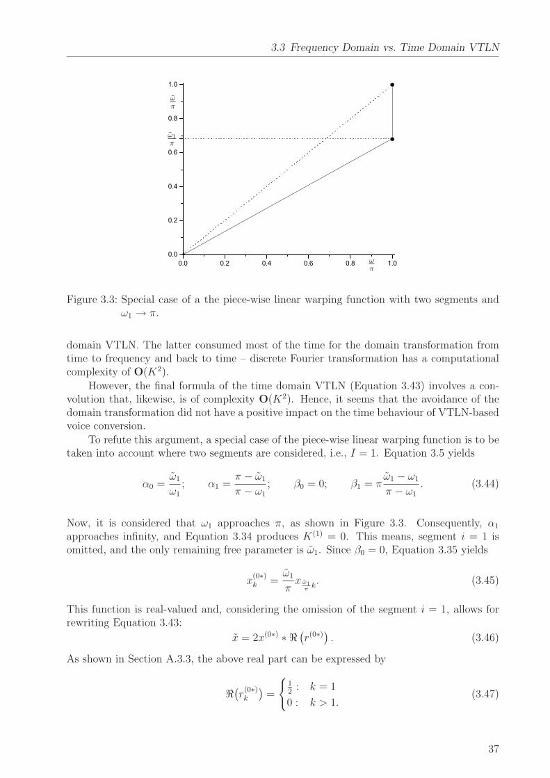
3.3 Frequency Domain vs. Time Domain VTLN
0.0 0.2 0.4 0.6 0.8 1.00.0
0.2
0.4
0.6
0.8
1.0
ωπ
. ωπ
. ω1
π
Figure 3.3: Special case of a the piece-wise linear warping function with two segments andω1 → π.
domain VTLN. The latter consumed most of the time for the domain transformation fromtime to frequency and back to time – discrete Fourier transformation has a computationalcomplexity of O(K2).
However, the final formula of the time domain VTLN (Equation 3.43) involves a con-volution that, likewise, is of complexity O(K2). Hence, it seems that the avoidance of thedomain transformation did not have a positive impact on the time behaviour of VTLN-basedvoice conversion.
To refute this argument, a special case of the piece-wise linear warping function is to betaken into account where two segments are considered, i.e., I = 1. Equation 3.5 yields
α0 =ω1
ω1
; α1 =π − ω1
π − ω1
; β0 = 0; β1 = πω1 − ω1
π − ω1
. (3.44)
Now, it is considered that ω1 approaches π, as shown in Figure 3.3. Consequently, α1
approaches infinity, and Equation 3.34 produces K(1) = 0. This means, segment i = 1 isomitted, and the only remaining free parameter is ω1. Since β0 = 0, Equation 3.35 yields
x(0∗)k =
ω1
πx ω1
πk. (3.45)
This function is real-valued and, considering the omission of the segment i = 1, allows forrewriting Equation 3.43:
x = 2x(0∗) ∗ ℜ(
r(0∗)) . (3.46)
As shown in Section A.3.3, the above real part can be expressed by
ℜ(
r(0∗)k
)
=
{
12
: k = 1
0 : k > 1.(3.47)
37
3 VTLN-Based Voice Conversion
Now, the convolution operator’s definition given by Equation 3.31 is inserted into Equa-tion 3.46 yielding the final result
xk = 2
[
k∑
n=1
x(0∗)n ℜ(r
(0∗)k−n+1) +
K∑
n=k+1
x(0∗)n ℜ(r
(0∗)k−n+1+K)
]
= 2x(0∗)k · 1
2=
ω1
πx ω1
πk. (3.48)
This means, for the special case considered in the above derivations, the convolution isomitted, and the computational complexity is reduced to O(K). An exact breakdown of thenumber of operations for this special case compared with frequency domain VTLN is givenin Table 3.1. Taking into account the example at the very beginning of Section 3.3, i.e.,K = 200, the proposed time domain VTLN accelerates computation by a factor of about40. In absolute terms, this corresponds to 1.28Mops/s.
3.3.4 Experiments
In the last section, it was shown that, for a special case, time domain VTLN significantlyaccelerates the computation. Now, it was important to investigate if this paradigm changewould perceptually affect the speech output. Therefore, both frequency- and time-domain-VTLN-based voice conversion were compared in terms of speech quality and performanceto change the voice identity. This was done using the MOS and the extended ABX testdescribed in Sections 2.5.2 and 2.5.3. For these subjective tests, 14 subjects, 12 of whomspecialists in speech processing, were invited.
From the Spanish synthesis corpus described in Section A.2.1, ten parallel utterances(about 40s) were randomly selected and aligned by means of dynamic time warping. For bothgender combinations, the parameter training according to Section 3.1 was performed. Then,frequency and time domain VTLN were applied to a random selection of 8 parallel utterancesof both genders (about 30s) which were different from those in the training data obtaininga total of 32 converted utterances. From these, 8 sentences were randomly selected in a waythat each gender/VTLN-type combination was represented by exactly two sentences. Thisrandomization was carried out again for each of the 14 participants. An overview about thetraining and testing data as well as the compared systems’ properties is given in Table 3.2.Table 3.3 reports the results of the MOS test and Table 3.4 those of the extended ABX testdepending on the VTLN technique and the gender combination.
3.3.5 Conclusion
The outcomes of the MOS test on speech quality in Table 3.3 certify a fair speech qualityfor both frequency- as well as time-domain-VTLN-based voice conversion. The conversionfrom the female to the male voice performs significantly better than the other way around.An analysis of the distortions and artifacts produced by the conversion algorithm showedthat most of them could be attributed to errors of the pitch tracker that achieved a higherperformance for female than for male speech confirming results of [Hoge & Kotnik+ 06].
This outcome, however, does not allow for the general conclusion that male-to-femaleconversion is the harder task, since comparing with experiments on databases involving othervoices suggests that the conversion has a stronger dependence on the particular processed
38
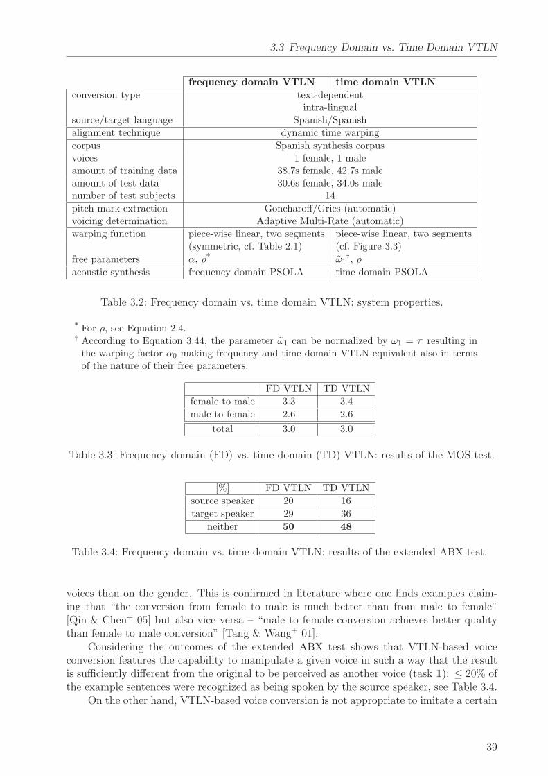
3.3 Frequency Domain vs. Time Domain VTLN
frequency domain VTLN time domain VTLN
conversion type text-dependentintra-lingual
source/target language Spanish/Spanish
alignment technique dynamic time warping
corpus Spanish synthesis corpusvoices 1 female, 1 maleamount of training data 38.7s female, 42.7s maleamount of test data 30.6s female, 34.0s malenumber of test subjects 14
pitch mark extraction Goncharoff/Gries (automatic)voicing determination Adaptive Multi-Rate (automatic)
warping function piece-wise linear, two segments piece-wise linear, two segments(symmetric, cf. Table 2.1) (cf. Figure 3.3)
free parameters α, ρ* ω1†, ρ
acoustic synthesis frequency domain PSOLA time domain PSOLA
Table 3.2: Frequency domain vs. time domain VTLN: system properties.
* For ρ, see Equation 2.4.† According to Equation 3.44, the parameter ω1 can be normalized by ω1 = π resulting in
the warping factor α0 making frequency and time domain VTLN equivalent also in termsof the nature of their free parameters.
FD VTLN TD VTLN
female to male 3.3 3.4
male to female 2.6 2.6
total 3.0 3.0
Table 3.3: Frequency domain (FD) vs. time domain (TD) VTLN: results of the MOS test.
[%] FD VTLN TD VTLN
source speaker 20 16
target speaker 29 36
neither 50 48
Table 3.4: Frequency domain vs. time domain VTLN: results of the extended ABX test.
voices than on the gender. This is confirmed in literature where one finds examples claim-ing that “the conversion from female to male is much better than from male to female”[Qin & Chen+ 05] but also vice versa – “male to female conversion achieves better qualitythan female to male conversion” [Tang & Wang+ 01].
Considering the outcomes of the extended ABX test shows that VTLN-based voiceconversion features the capability to manipulate a given voice in such a way that the resultis sufficiently different from the original to be perceived as another voice (task 1): ≤ 20% ofthe example sentences were recognized as being spoken by the source speaker, see Table 3.4.
On the other hand, VTLN-based voice conversion is not appropriate to imitate a certain
39
3 VTLN-Based Voice Conversion
speaker’s voice (task 2): The results report that only around a third of the examples wereperceived to be uttered by the target speaker.
Finally, the experimental results show that the two compared conversion techniquesbased on frequency and time domain VTLN perform very similarly in terms of both speechquality and voice identity. The time-domain-VTLN-based technique, however, is consider-ably faster (in the example discussed above by a factor of about 40).
3.4 On Generating Several Well-Distinguishable Voices
The results of the last section showed that VTLN-based voice conversion is able to changea source speaker’s voice such that it is perceived to be another voice. However, would itbe possible to produce two voices that are perceived to be different from the source voiceand also from each other, or even more? This capability could play a role for scenarios likein speech-to-speech translation for parliamentary speeches as in the project TC-Star (cf.Section A.1) where several politicians have to be clearly distinguished.
Consequently, this section is to investigate the characteristics of VTLN-based voiceconversion with respect to the production of well-distinguishable voices. In doing so, thespecial case discussed in the last section is to be used, i.e., the number of parameters is limitedto two, the warping factor α and the ratio ρ between the mean fundamental frequencies afterand before the conversion. To simplify matters, they are combined in the vector v = (α, ρ).
3.4.1 On the Naturalness of Converted Voices
It is obvious that only parameter values inside a certain range result in reasonable, i.e.naturally sounding voices. E.g., setting v = (1, 1) does not change the voice at all andshould result in the maximum naturalness when distortions by the analysis-synthesis systemcan be neglected. On the other hand, extreme values as r → ∞ produce artificial or evenirrecognizable voices.
Hence, at the beginning, the relation between the parameter settings and the voices’naturalness was to be investigated. This was done by performing a subjective test on thenaturalness of the converted speech. The corpus used in the following experiments is theGerman synthesis corpus described in Section A.2.2. From both the female and the malespeaker, 25 utterances were randomly selected and converted based on the parameters dis-played in Figure 3.4 which were determined by means of informal listening tests.
Now, 11 subjects were asked to rate the naturalness of converted speech samples on anMOS scale between 1 (artificial) and 5 (natural) based on the following instructions:
“You listen to 50 speech samples. In this experiment, you are to rank the nat-uralness of voices. Please, do not pay attention to the recording conditions, thesound or synthesis quality of the samples, or to the speaking style; we are justinterested in whether you think the voices sound as if uttered by a real person.”
Table 3.5 shows the system properties of this experiment. From the resulting naturalnessscores belonging to the 25 parameter vectors of the female and the male speaker, respectively,an estimate for the score in the whole v space was produced by applying a two-dimensionalinterpolation based on Delaunay triangulation [Preparata & Shamos 85] to the scattereddata. Figure 3.5 shows the results.
40
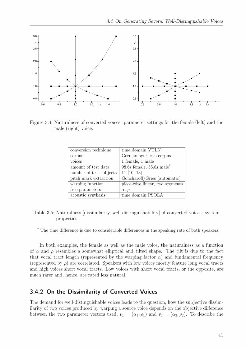
3.4 On Generating Several Well-Distinguishable Voices
0.6 0.8 1.0 1.2 1.4
0.5
1.0
1.5
2.0
2.5
3.0
0.6 0.8 1.0 1.2 1.4
0.5
1.0
1.5
2.0
2.5
3.0
α α
. ρ ρ
Figure 3.4: Naturalness of converted voices: parameter settings for the female (left) and themale (right) voice.
conversion technique time domain VTLNcorpus German synthesis corpusvoices 1 female, 1 male
amount of test data 98.6s female, 55.8s male*
number of test subjects 11 [10, 13]pitch mark extraction Goncharoff/Gries (automatic)warping function piece-wise linear, two segmentsfree parameters α, ρ
acoustic synthesis time domain PSOLA
Table 3.5: Naturalness [dissimilarity, well-distinguishability] of converted voices: systemproperties.
* The time difference is due to considerable differences in the speaking rate of both speakers.
In both examples, the female as well as the male voice, the naturalness as a functionof α and ρ resembles a somewhat elliptical and tilted shape. The tilt is due to the factthat vocal tract length (represented by the warping factor α) and fundamental frequency(represented by ρ) are correlated. Speakers with low voices mostly feature long vocal tractsand high voices short vocal tracts. Low voices with short vocal tracts, or the opposite, aremuch rarer and, hence, are rated less natural.
3.4.2 On the Dissimilarity of Converted Voices
The demand for well-distinguishable voices leads to the question, how the subjective dissim-ilarity of two voices produced by warping a source voice depends on the objective differencebetween the two parameter vectors used, v1 = (α1, ρ1) and v2 = (α2, ρ2). To describe the
41
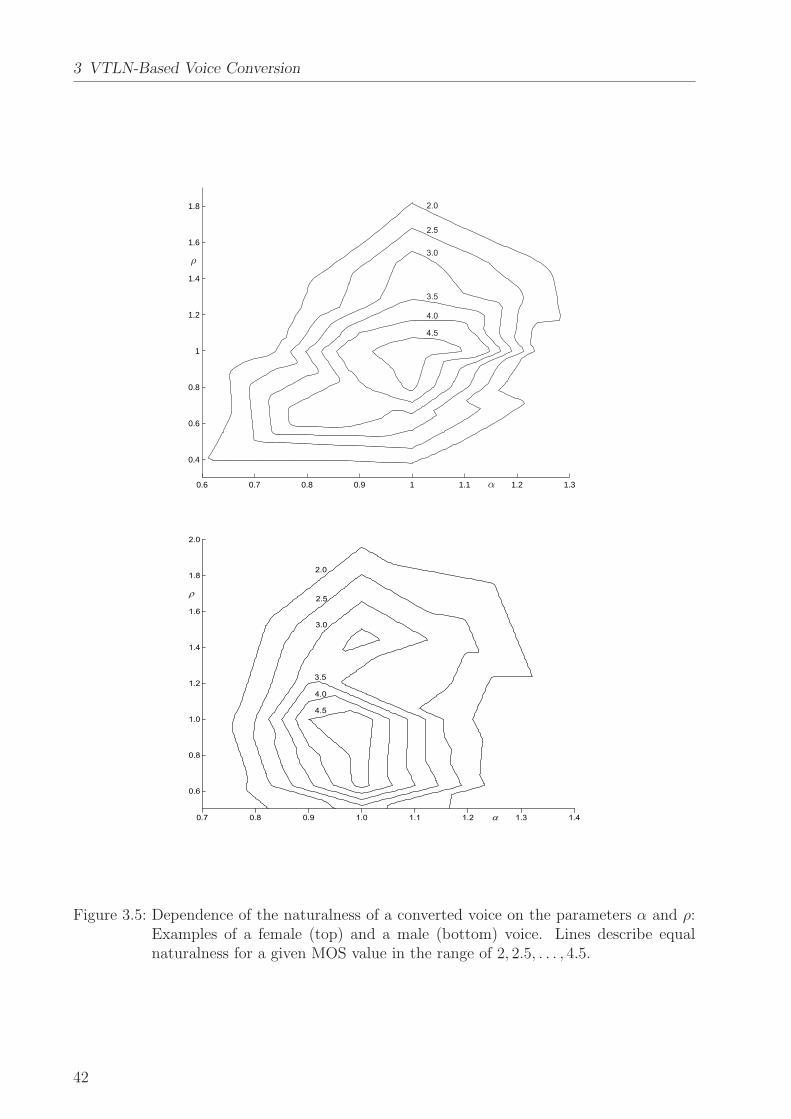
3 VTLN-Based Voice Conversion
.........
0.6 0.7 0.8 0.9 1 1.1 1.2 1.3
0.4
0.6
0.8
1
1.2
1.4
1.6
1.8 2.0
2.5
3.0
3.5
4.0
4.5
α
. ρ
0.7 0.8 0.9 1.0 1.1 1.2 1.3 1.4
0.6
0.8
1.0
1.2
1.4
1.6
1.8
2.0
2.0
2.5
3.0
3.5
4.0
4.5
Figure 3.5: Dependence of the naturalness of a converted voice on the parameters α and ρ:Examples of a female (top) and a male (bottom) voice. Lines describe equalnaturalness for a given MOS value in the range of 2, 2.5, . . . , 4.5.
42
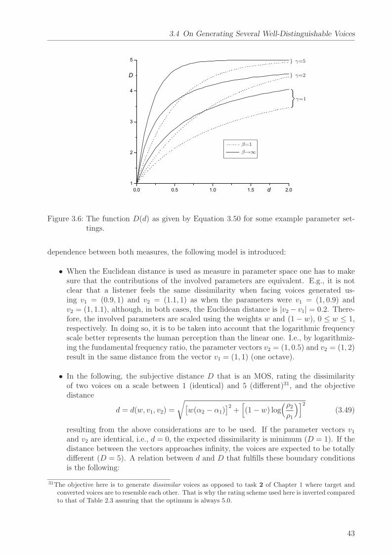
3.4 On Generating Several Well-Distinguishable Voices
.........
0.0 0.5 1.0 1.5 2.01
2
3
4
5
d
D
. β=1
. β→∞
. } γ=5
. } γ=2
.
}
γ=1
Figure 3.6: The function D(d) as given by Equation 3.50 for some example parameter set-tings.
dependence between both measures, the following model is introduced:
• When the Euclidean distance is used as measure in parameter space one has to makesure that the contributions of the involved parameters are equivalent. E.g., it is notclear that a listener feels the same dissimilarity when facing voices generated us-ing v1 = (0.9, 1) and v2 = (1.1, 1) as when the parameters were v1 = (1, 0.9) andv2 = (1, 1.1), although, in both cases, the Euclidean distance is |v2 − v1| = 0.2. There-fore, the involved parameters are scaled using the weights w and (1 − w), 0 ≤ w ≤ 1,respectively. In doing so, it is to be taken into account that the logarithmic frequencyscale better represents the human perception than the linear one. I.e., by logarithmiz-ing the fundamental frequency ratio, the parameter vectors v2 = (1, 0.5) and v2 = (1, 2)result in the same distance from the vector v1 = (1, 1) (one octave).
• In the following, the subjective distance D that is an MOS, rating the dissimilarityof two voices on a scale between 1 (identical) and 5 (different)31, and the objectivedistance
d = d(w, v1, v2) =
√
[
w(α2 − α1)]2
+[
(1 − w) log(ρ2
ρ1
)]2
(3.49)
resulting from the above considerations are to be used. If the parameter vectors v1
and v2 are identical, i.e., d = 0, the expected dissimilarity is minimum (D = 1). If thedistance between the vectors approaches infinity, the voices are expected to be totallydifferent (D = 5). A relation between d and D that fulfills these boundary conditionsis the following:
31The objective here is to generate dissimilar voices as opposed to task 2 of Chapter 1 where target andconverted voices are to resemble each other. That is why the rating scheme used here is inverted comparedto that of Table 2.3 assuring that the optimum is always 5.0.
43
3 VTLN-Based Voice Conversion
female male
γ 4.7 3.2w 0.5 0.7
ε(w,∞, γ) 0.3 0.4
Table 3.6: Parameters of the dissimilarity model.
D(d) = 5 ·[
1 −(
γ
βd+
β
√
5
4
)−β]
; γ, β > 0. (3.50)
Using the maximum and minimum parameter values for α and ρ given in Figure 3.4and inserting these values into Equation 3.49 yields d < 2 for the current experimentalsetup. Figure 3.6 displays the function D(d) for 0 ≤ d ≤ 2 for some example parametersettings.
In order to determine the unknown model parameters w, β, and γ, another subjective testwas performed; for the system settings, see Table 3.5. This time, 10 subjects were asked torate the dissimilarity of J = 24 pairs of voices derived from the aforementioned corpus. Thecompared voices were the same as generated for the naturalness experiment in Section 3.4.1.A pair always consisted of voices derived from opposite parameter vectors with respect to theneutral element v = (1, 1), see Figure 3.4. Averaging over the participants, this resulted in ascore Dj for each parameter vector pair v1j, v2j, 12 for each gender. Applying Equations 3.49and 3.50, the model parameters are estimated by minimizing the root mean square betweenthe model D(d(v1j, v2j)) and the subjective scores Dj:
(w, β, γ) = arg minw′,β′,γ′
ε(w′, β′, γ′) with (3.51)
ε(w, β, γ) =
√
√
√
√
1
J
J∑
j=1
[
D(
d(w, v1j, v2j), β, γ)
−Dj
]2
. (3.52)
It turns out that for the considered scores, β becomes sufficiently large to approximateEquation 3.50 by its limit for β → ∞:
limβ→∞
Dβ(d) = 5 ·[
1 − limβ→∞
(
γ
βd+
β
√
5
4
)−β]
= 5 ·[
1 − exp
(
limβ→∞
[
ln
(
γ
βd+
β
√
5
4
)−β])]
. (3.53)
.
44
3.4 On Generating Several Well-Distinguishable Voices
Substituting β = 1b
and applying l’Hopital’s rule yields
limβ→∞
Dβ(d) = 5 ·[
1 − exp
(
limb→0
ln[
γdb+(
54
)
b]
−b
)]
= 5 ·[
1 − exp
(
limb→0
γd+(
54
)
b ln 54
−γdb−(
54
)
b
)]
= 5 ·[
1 − exp(
−γd− ln 54
)]
= 5 − 4e−γd; γ > 0. (3.54)
In Table 3.6, for both genders, the determined parameters are displayed. In order to assessthe performance of the model, we also include the (absolute) model error ε(w,∞, γ), i.e. theroot mean square obtained by using the optimized parameters γ and w, see Equations 3.51and 3.52.
3.4.3 Generating Well-Distinguishable Voices
As argued in Section 3.4.1, the objective of the current investigations is to generate a certainnumber of well-distinguishable voices, while taking into account that the produced voicesfeature a reasonable naturalness as discussed in Section 3.4.2. As an example, for each ofthe given voices, it is to be shown that 5 voices can be created by applying VTLN-basedvoice conversion to the source voice such that their naturalness and dissimilarity scores areat least 3.0:
• At first, the area of the parameter space that provides a naturalness score greater than3.0 is determined (cf. contour lines in Figure 3.5).
• Then, 5 vectors v51 are distributed inside the region so that the minimum distance
between two of these vectors d(vi, vj) becomes maximal:
v51 = arg max
v′5′1
mini, j = 1, . . . , 5
i 6= j
d(v′i, v′j) . (3.55)
This is done by
– rasterizing the region obtaining a discrete set of allowed vectors,
– determining the centroid of these vectors, and,
– as initial setting, assigning the centroid position to all the vectors v′5′1.
– Now, the vector v′1 is moved to the position of that allowed vector which has themaximum distance to the closest neighbor.
– This is done equivalently with the remaining vectors v′5′2.
– The process is iterated by moving v′1 to the position of that allowed vector whichhas the maximum distance to the closest neighbor, and so on, until v
′5′1 remain
constant.
45
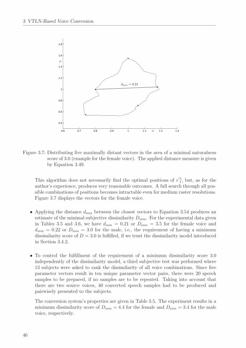
3 VTLN-Based Voice Conversion
.........
0.6 0.7 0.8 0.9 1 1.1 1.2 1.3
0.4
0.6
0.8
1
1.2
1.4
1.6
1.8
dmin = 0.21
α
. ρ
Figure 3.7: Distributing five maximally distant vectors in the area of a minimal naturalnessscore of 3.0 (example for the female voice). The applied distance measure is givenby Equation 3.49.
This algorithm does not necessarily find the optimal positions of v′5′1, but, as for the
author’s experience, produces very reasonable outcomes. A full search through all pos-sible combinations of positions becomes intractable even for medium raster resolutions.Figure 3.7 displays the vectors for the female voice.
• Applying the distance dmin between the closest vectors to Equation 3.54 produces anestimate of the minimal subjective dissimilarity Dmin. For the experimental data givenin Tables 3.5 and 3.6, we have dmin = 0.21 or Dmin = 3.5 for the female voice anddmin = 0.22 or Dmin = 3.0 for the male, i.e., the requirement of having a minimumdissimilarity score of D = 3.0 is fulfilled, if we trust the dissimilarity model introducedin Section 3.4.2.
• To control the fulfillment of the requirement of a minimum dissimilarity score 3.0independently of the dissimilarity model, a third subjective test was performed where13 subjects were asked to rank the dissimilarity of all voice combinations. Since fiveparameter vectors result in ten unique parameter vector pairs, there were 20 speechsamples to be prepared, if no samples are to be repeated. Taking into account thatthere are two source voices, 40 converted speech samples had to be produced andpairwisely presented to the subjects.
The conversion system’s properties are given in Table 3.5. The experiment results in aminimum dissimilarity score of Dmin = 4.4 for the female and Dmin = 3.4 for the malevoice, respectively.
46
3.4 On Generating Several Well-Distinguishable Voices
3.4.4 Conclusion
This section’s considerations aimed at investigating the ability of VTLN-based voice conver-sion to produce several well-distinguishable voices from one source voice. For that purpose,the dependence between the parameter settings (the warping factor α and the ratio betweenthe means of the fundamental frequency of two compared voices ρ) and naturalness as wellas dissimilarity of the produced voices was experimentally investigated. For the latter, i.e.the relation between the respective parameters of two compared voices (α1, ρ1 and α2, ρ2)and the perceived dissimilarity in terms of an MOS, a model equation was introduced thatresulted in a model error of a root mean square of less than 0.4 on the German synthesiscorpus which is relatively small compared with the range of the MOS (1.0 to 5.0).
It was shown that in the region of a naturalness of at least 3.0 on an MOS scale, fiveparameter sets could be distributed such that the dissimilarity model certified a minimumdissimilarity of 3.0. This result could be confirmed by conducting an experiment where foreach voice pair the dissimilarity was subjectively assessed.
47

3 VTLN-Based Voice Conversion
48
4 Residual Prediction
In Section 2.4.3, four approaches to residual prediction were described, and their drawbackswere identified as summarized in Table 4.1. Both the residual codebook technique and resid-ual selection were based on the assumption that the correlation between feature vectors andunderlying residual is strong enough to reliably predict the residuals based on the featuresonly. However, the following gedankenexperiment weakens this assumption, in particularwith respect to residual selection:
Let us consider a number of natural residuals extracted from the frames of a speechsample and just one feature vector derived from a randomly chosen frame. Now, we filterthe residuals by means of the single available feature vector’s coefficients producing a numberof time frames that, dependent on the nature of the underlying residual, feature individualcharacteristics32. When, however, such candidates, i.e. frames that have identical featurevectors but varying residuals, appeared in the residual selection table, this would have afatal effect: If the residual of a feature vector identical to the one used in the experimentwas to be predicted, one of the many varying residuals would be selected by chance, maybean inadequate one, resulting in unintentional perceptive effects as artifacts.
This gedankenexperiment challenges the validity of the correlation between feature vec-tors and residuals and is an exaggeration of the real-world situation, since many of theartificially created feature-vector/residual combinations do not appear in real speech data.Still, the phenomenon of selecting inappropriate residuals given a sequence of natural fea-ture vectors has to be taken into account, as experiments on residual selection resulting ina considerable number of artifacts in voiced speech regions show, see report in Section 4.1.
In addition to the correlation insufficiency, both the residual codebook method andresidual selection deal with magnitude and phase spectra in different processes frequentlyleading to mismatches between both spectral components and, finally, to a “rough”[Kain & Macon 01] or “harsh” [Ye & Young 04a] quality of the converted signal. This dis-sertation investigates three solutions to these dilemmas.
4.1 Residual Smoothing
4.1.1 Residual Smoothing as an Integral Approach
Residual smoothing tries to simultaneously handle inaccuracies of the residual selection dueto a lack of correlation and mismatches between magnitude and phase spectra of the predictedresiduals. Similar to the integral approach to frequency warping based on complex-valuedspline interpolation (cf. Section 2.4.3), the author assumed that the most reliable approach
32 Informal listening tests even suggest that, if these time frames are concatenated using PSOLA, the textcontent of the resulting speech can still be recognized, and much of the speaker individuality survives.This confirms that the residuals contain important speaker-dependent information.
4 Residual Prediction
technique drawbacks
vocoder synthetic soundsource residuals a third speaker is createdresidual codebook only a few prototypes, phase mismatchesresidual selection artifacts, phase mismatches
Table 4.1: Residual prediction techniques and their drawbacks.
for dealing with the phase spectra is to not separate them from the magnitude spectra, but,instead, treat them as one complex-valued spectrum.
The proposed time-variant residual smoothing is based on the residual selection tech-nique, in particular on Equation 2.16 which delivers the most probable residual spectrum rfor a given feature vector x by selecting from a table with all residuals rM
1 seen in training.Here, rm are complex-valued spectra normalized to a constant number of spectral lines asdiscussed in Section 2.4.3. In the following, rK
1 is a sequence of residual spectra generatedby means of residual selection given the sequence of converted feature vectors xK
1 .As already mentioned in Section 2.4.3, in unvoiced frames, the residual is expected to be
white with random phases, thus, “chaotic”, whereas in voiced parts, the signal is expectedto be pseudo-periodic. Hence, significant changes in the residual waveform within voicedparts, e.g. due to an insufficient correlation between the residual and the converted featurevector, would be fatal and result in clearly audible artifacts.
The presented solution to this problem is a voicing-dependent residual smoothing whichmakes sure that neighbored residuals resemble each other in voiced regions but does notchange anything in unvoiced regions hardly affected by the aforementioned signal deterio-rations. Again, as in Sections 2.3.4 and 3.1, these considerations are not based on a hardvoiced/unvoiced decision but on the voicing degree 0 ≤ vk ≤ 1 estimated for each framek = 1, . . . , K to be converted.
The proposed smoothing assumes that the residual at a position k is influenced by allits neighbors. This influence is the stronger the closer the neighbor is to the position k. Thisis achieved by summing up over all residuals produced by means of the residual selectionparadigm weighted with a normal distribution whose mean coincides with the position k,to make sure that the contribution of the current position is strongest, and whose standarddeviation linearly depends on the voicing degree of the kth frame
σk = vkσ0 (4.1)
where the norm standard deviation σ0 determines the smoothing strength. It is an empiri-cally determined constant adjusting the tradeoff between smoothing away the typical residualselection artifacts and producing a too smooth sound of the voice by raising the voicing ofhardly voiced speech portions, similar to the effect of applying PSOLA to unvoiced soundsdiscussed in Section 2.3.4. Thus, the smoothed residual at the position k is expressed by:
r′k =
K∑
κ=1
N (κ|k, σk) · rκ
K∑
κ=1
N (κ|k, σk)
, (4.2)
50
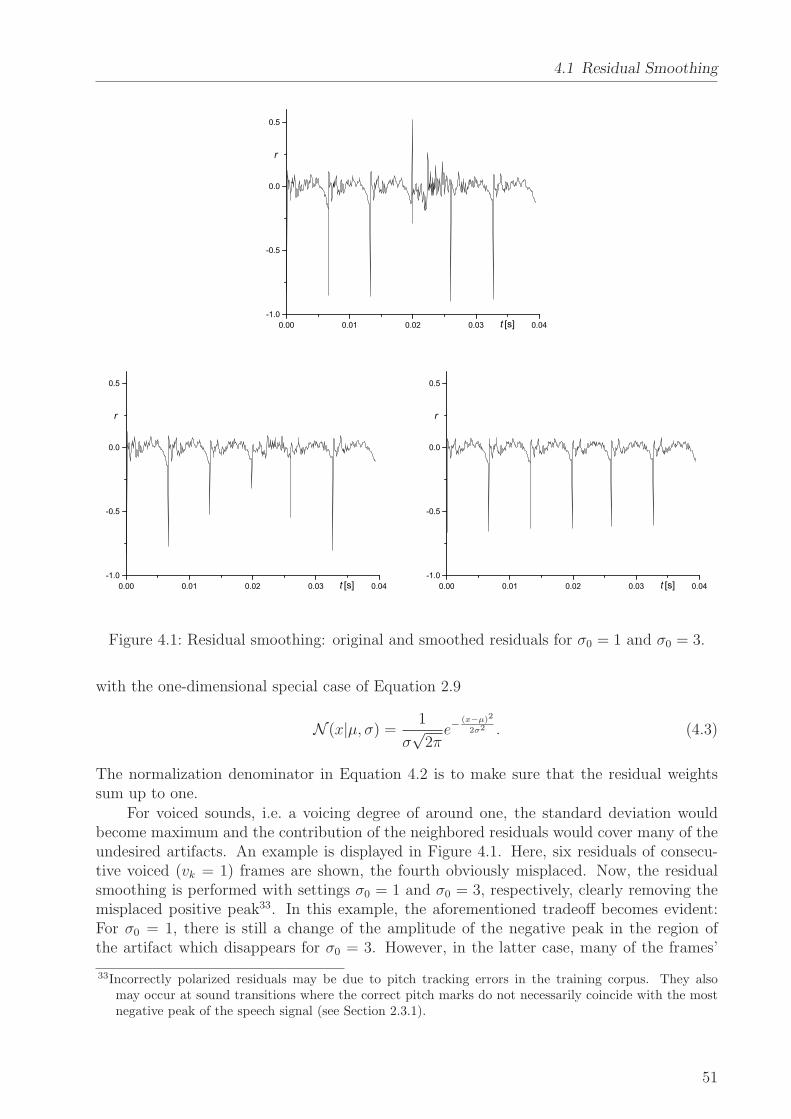
4.1 Residual Smoothing
0.00 0.01 0.02 0.03 0.04-1.0
-0.5
0.0
0.5
r
t [s]
0.00 0.01 0.02 0.03 0.04-1.0
-0.5
0.0
0.5
r
t [s] 0.00 0.01 0.02 0.03 0.04
-1.0
-0.5
0.0
0.5
r
t [s]
Figure 4.1: Residual smoothing: original and smoothed residuals for σ0 = 1 and σ0 = 3.
with the one-dimensional special case of Equation 2.9
N (x|µ, σ) =1
σ√
2πe−
(x−µ)2
2σ2 . (4.3)
The normalization denominator in Equation 4.2 is to make sure that the residual weightssum up to one.
For voiced sounds, i.e. a voicing degree of around one, the standard deviation wouldbecome maximum and the contribution of the neighbored residuals would cover many of theundesired artifacts. An example is displayed in Figure 4.1. Here, six residuals of consecu-tive voiced (vk = 1) frames are shown, the fourth obviously misplaced. Now, the residualsmoothing is performed with settings σ0 = 1 and σ0 = 3, respectively, clearly removing themisplaced positive peak33. In this example, the aforementioned tradeoff becomes evident:For σ0 = 1, there is still a change of the amplitude of the negative peak in the region ofthe artifact which disappears for σ0 = 3. However, in the latter case, many of the frames’
33Incorrectly polarized residuals may be due to pitch tracking errors in the training corpus. They alsomay occur at sound transitions where the correct pitch marks do not necessarily coincide with the mostnegative peak of the speech signal (see Section 2.3.1).
51
4 Residual Prediction
individual characteristics have disappeared, and all displayed residuals look fairly similar toeach other tending to produce less natural speech.
In the opposite case, i.e. for unvoiced frames, the voicing degree and, consequently, thestandard deviation σk approach 0, and Equation 4.2 becomes
limσk→0
r′k =
K∑
κ=1
∆(κ− k) · rκ
K∑
κ=1
∆(κ− k)
= rk, (4.4)
with the Dirac delta function as the limit of the normal distribution according to [Arfken 85]:
limσ→0
N (x|µ, σ) = ∆(x− µ). (4.5)
That is, in unvoiced frames, the residuals remain unchanged as delivered by the residualselection.
4.1.2 On the Correlation between Source and Target Residuals
The above example (Figure 4.1) suggests that residual smoothing is a strong technique tosuppress artifacts. As argued in Section 4.1.1, the drawback of this technique is the tendencyto oversmoothing, yielding a loss of naturalness. If there were means to avoid the artifactsalready before applying the smoothing, the smoothing strength σ0 could be reduced leadingto a higher naturalness of the generated speech.
As mentioned before, there are two error sources of the residual selection, the potentialweakness of the conversion function, and consequently erroneous converted feature vectors,and the insufficient correlation between feature vectors and respective residuals. The detourvia imperfect converted feature vectors could be avoided by predicting the target residualsbased on the source residuals only, expecting a considerable correlation between them. Theidea was to derive a vector representation from the residuals themselves and use them insteadof the line-spectral-frequency-based feature vectors x and y required in residual selectionEquation 2.16.
After testing a set of residual vector representations using informal listening tests, itturned out that particularly reliable is a vector based on the component-wise absolute valueof the time domain representation r of a given residual vector reduced by the constantcomponent (its mean r) and normalized to a constant number of spectral lines and to anenergy of 1.0:
R(r) =abs(r − r)
|r − r| . (4.6)
Returning to Equation 2.16, the converted vector x would be replaced by the current sourceresidual vector R(r) and the target vector ym by the vector representation of the raw targetresidual R(rm):
r = arg minr′=r1,...,rM
∣
∣R(r) −R(r′)∣
∣. (4.7)
52
4.1 Residual Smoothing
4.1.3 Experiments
This section describes a comparative study of most of the techniques introduced in Sec-tion 2.4.3 and in this chapter investigating both the techniques’ speech quality and theircapability of changing the voice identity from source to target. The following techniques arecompared:
• copying source residuals,
• residual codebook method,
• residual selection,
• residual smoothing based on the feature criterion (Equation 2.16),
• residual smoothing* based on the residual criterion (Equation 4.7).
Evaluation corpus was the Spanish synthesis corpus described in Section A.2.1. From thiscorpus, ten parallel utterances were randomly selected for training and three utterances fortesting. The training was performed according to the paradigm described in Section 2.4.2estimating the linear transformation parameters. The free parameters of featurization andGaussian mixture model (line spectral frequency order, number of Gaussian mixtures, typeof covariance matrix) were chosen in accordance with relevant literature [Kain 01] and takinginto account numerical instabilities that arise when the number of parameters to be estimatedis too large [Sundermann & Bonafonte+ 04a]. Details of this experiment’s system propertiescan be found in Table 4.2.
As subjective evaluation criteria, the mean opinion score was used for assessing speechquality (see Section 2.5.3), and the extended ABX test served for determining the similarityof converted and target voice (cf. Section 2.5.2). The results of the evaluation are shown inTables 4.3 and 4.4.
4.1.4 Conclusion
As for the speech quality reported in Table 4.3, a well-known speech synthesis rule claimingthat less (signal processing) is more (speech quality) [Beutnagel & Conkie+ 99] lets unpro-cessed source residuals achieve a 0.9 MOS points better result than the best of its com-petitors. Among the remaining techniques, residual smoothing outperforms the others interms of speech quality, although the absolute MOS (2.6) shows that there is still a need forimprovement.
Addressing the similarity of converted and target voice, one finds that all assessedtechniques succeed in converting the source voice to the target voice to more than 70%, cf.Table 4.4. The only exception are the source residuals where the majority of the listeners hadthe impression of hearing a third speaker as also found in former studies, see Section 2.4.3.Residual smoothing shows the highest conversion performance.
Finally, the question on which of the correlations, that between converted feature vec-tors and underlying residuals (conventional) or that between source and target residuals(proposed), achieves better results, is to be addressed. The outcomes of MOS as well as
53
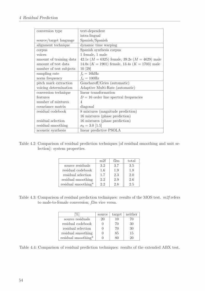
4 Residual Prediction
conversion type text-dependentintra-lingual
source/target language Spanish/Spanish
alignment technique dynamic time warping
corpus Spanish synthesis corpusvoices 1 female, 1 maleamount of training data 42.1s (M = 6325) female, 39.2s (M = 4629) maleamount of test data 14.0s (K = 1901) female, 13.4s (K = 1703) malenumber of test subjects 10 [29]
sampling rate fs = 16kHznorm frequency fn = 100Hz
pitch mark extraction Goncharoff/Gries (automatic)voicing determination Adaptive Multi-Rate (automatic)
conversion technique linear transformationfeatures D = 16 order line spectral frequenciesnumber of mixtures 4covariance matrix diagonal
residual codebook 8 mixtures (magnitude prediction)16 mixtures (phase prediction)
residual selection 16 mixtures (phase prediction)residual smoothing σ0 = 3.0 [1.5]
acoustic synthesis linear predictive PSOLA
Table 4.2: Comparison of residual prediction techniques [of residual smoothing and unit se-lection]: system properties.
m2f f2m total
source residuals 3.2 3.7 3.5residual codebook 1.6 1.9 1.8residual selection 1.7 2.3 2.0
residual smoothing 2.2 2.9 2.6residual smoothing* 2.2 2.8 2.5
Table 4.3: Comparison of residual prediction techniques: results of the MOS test. m2f refersto male-to-female conversion; f2m vice versa.
[%] source target neither
source residuals 20 10 70residual codebook 0 70 30residual selection 0 70 30
residual smoothing 0 85 15residual smoothing* 0 80 20
Table 4.4: Comparison of residual prediction techniques: results of the extended ABX test.
54
4.2 Unit Selection
extended ABX test do not show significant differences between either criteria, both correla-tions seem to be equivalently appropriate to the task. Since the conventional paradigm hasa wider range of application (in addition to its use for voice conversion, it can be appliedto HMM-based speech synthesis where only target feature vectors are available to predictfrom, cf. comments in Section 2.4.3), the following investigations of this thesis will be basedon the feature criterion, i.e. the conventional approach.
4.2 Unit Selection
The conclusion of Section 4.1.4 was that both the transformed feature vector’s and the sourceresidual’s correlation to the target residual is not sufficient to produce artifact-free speechbased on the residual selection paradigm. To suppress these artifacts, residual smoothinghas to be applied tending to reduce the speech naturalness by oversmoothing.
If there were a technique for more reliably selecting residuals from the training databaseso that the selected residual sequence rK
1 already contains less artifacts, one could reduce thesmoothing strength σ0 and, hence, improve the quality of the converted speech. Certainly,the most appropriate residual sequence is one that was seen in training and that fulfills theoptimization criterion of Equation 2.16 at the same time. Of course, this will only apply ifthe converted feature sequence xK
1 is identical to a feature sequence seen in training. Sincethis will hardly be the case, these conditions should be weakened, and the residual sequenceshould be allowed to be composed of several subsequences seen in training whose endingsfit together. Furthermore, also suboptima of Equation 2.16 should be taken into account inorder to obtain subsequences of reasonable lengths. This approach is called unit selection, atechnique that is widely used in concatenative speech synthesis [Hunt & Black 96].
Generally, in the unit selection framework, two cost functions are defined. The targetcost Ct(uk, tk) is an estimate of the difference between the database unit uk and the targettk it is supposed to represent. The concatenation cost Cc(uk−1, uk) is an estimate of thequality of a join between the consecutive units uk−1 and uk.
In speech synthesis, the considered units are subphones [Donovan & Woodland 95],phones [Taylor & Black+ 98], or syllables [Lewis & Tatham 99], whereas in the residual pre-diction case, the base unit length is set to be a single speech frame, since this allows for beingindependent of additional linguistic information about the processed speech as the phoneticsegmentation. Furthermore, the cost functions can easily be defined by interpreting theresiduals as database units, i.e., u = r.
In the following sections, the properties of the cost functions used for unit-selection-based residual prediction are described. Moreover, it is shown how the final residual sequenceis produced.
4.2.1 Target and Concatenation Cost Function
Similar to the residual selection described in Equation 2.16, the appropriateness of a residualrm seen in training for being selected for the kth frame is determined based on the distancebetween the corresponding feature vector ym and the one representing the properties of thekth converted frame, xk. Furthermore, fundamental frequency and energy of the consideredresidual are to be taken into account. This is to minimize the extent of signal processingto produce the prosodic characteristics of the converted speech and, thus, avoid distortions
55
4 Residual Prediction
of the natural waveform. According to [Hunt & Black 96], the target cost Ct is calculatedas the weighted sum of the distances between the considered features of the target and thecandidate:
Ct(u, t) = Ct(
rm, (xk, f0k, Sk))
= w1d(
ym, xk
)
+ w2d(
f0(rm), f0k
)
+ w3d(
|rm|2, Sk
)
. (4.8)
f0k and Sk are target fundamental frequency and energy that, in the case of residual predic-tion for voice conversion, can be derived from the respective parameters of the source speechframe:
• the fundamental frequency is linearly normalized to match the target average by meansof the factor ρ (cf. Section 2.3.4),
• the energy is expected to be equivalent to the source residual energy |rk|2.
This finally yields34
Ct(u, t) = w1d(
ym, xk
)
+ w2d(
f0(rm), ρf0(rk))
+ w3d(
|rm|2, |rk|2)
= Ct(k,m). (4.9)
For the weights holds (see also Equation 4.12)
w1 + w2 + w3 ≤ 1; w1, w2, w3 ≥ 0. (4.10)
This makes sure that the sum of the cost functions’ weights including that of the belowdiscussed concatenation cost is always 1.
d is the Mahalanobis distance that compensates for differences of range and amount ofvariation between the features used in Equation 4.8:
d(x, y) =√
(x− y)′Σ−1(x− y) (4.11)
where Σ is the covariance matrix computed using the respective features of all residuals seenin training.
The cost for concatenating the residuals rm and rn is defined using the normalizedresidual representation R(r) given in Equation 4.6:
Cc(m,n) = (1 − w1 − w2 − w3) ·∣
∣R(rm) −R(rn)∣
∣
2. (4.12)
When m and n refer to successive frames in the training data, i.e., n = m + 1 the concate-nation should be optimal, hence, it is defined
Cc(m,m+ 1) = 0. (4.13)
For the sake of completeness, furthermore, it is defined
Cc(0,m) = 0. (4.14)
34Note that rm is the mth target residual of the training data and rk is the kth source residual of the datato be converted. Consequently, the case m = k does not mean that both residuals are identical.
56
4.2 Unit Selection
4.2.2 Finding the Optimal Residual Sequence
The sought-after residual sequence rK1 is determined by minimizing the sum of the target
and concatenation costs applied to an arbitrarily selected sequence from the set of residualsseen in training:
rk = rmkfor k = 1, . . . , K with
mK1 = arg min
m′K′1
K∑
k=1
[
Ct(k,m′k) + Cc(m′
k−1,m′k)]
; m′k ∈ {1, . . . ,M}. (4.15)
The arbitrarily selected residual sequence is given by the index sequence m′K′1 . As for its
definition, there are MK different index sequences making the problem intractable at firstglance. However, it is observed that this formula which is a sum over addends that onlydepend on the two successive variables m′
k−1 and m′k has the same structure as Equation 3.13
proven to be resolvable by means of dynamic programming. Nevertheless, it turns out thatit still requires a high computational effort: The full solution of Equation 4.15 results in
O ≈ K ·M2 ·(
8D2 + 4D + 6fs
fn
)
ops. (4.16)
For this formula’s respective parameter values from the experimental corpus used in thiswork, see Table 4.2. As example, male-to-female conversion is to be considered which is com-putationally more expensive, since Equation 4.16 is dominated by the variable M (quadratic)as opposed to K (linear).
When these example parameter settings are used and the computation is run on acomputer that executes 1Gops/s it would take around 58 hours, i.e., it operates with 15,600times real time. In order to build a real-time system, ways to simplify the algorithm mustbe searched for:
• By introducing a pruning that only considers the 5 best hypotheses, the real-timefactor can be reduced to RTF = 12.3.
• Instead of utilizing the Mahalanobis distance (Equation 4.11), the Euclidean distancecan be applied without noticeably affecting the residual prediction quality (RTF = 4.4).
• The calculation of the concatenation cost in Equation 4.12 is restricted to the first of thetwo signal periods contained in the processed residuals, cf. Section 2.3.4 (RTF = 2.1).
• The norm frequency fn used to transform the residuals to vectors of identical lengths,cf. Section 2.4.3, can be duplicated without noticeably affect the behavior of the con-catenation cost function (RTF = 1.3).
• Taking into account that almost half of the durations of the speech signal to be con-verted and of that used for training is actually non-speech (silence or noise), we obtaina real-time factor of 0.3.
Consequently, at least on fast computers, the algorithm is real-time-able.
57
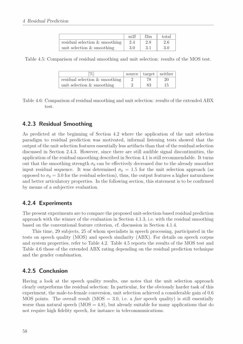
4 Residual Prediction
m2f f2m total
residual selection & smoothing 2.4 2.8 2.6unit selection & smoothing 3.0 3.1 3.0
Table 4.5: Comparison of residual smoothing and unit selection: results of the MOS test.
[%] source target neither
residual selection & smoothing 2 78 20unit selection & smoothing 2 83 15
Table 4.6: Comparison of residual smoothing and unit selection: results of the extended ABXtest.
4.2.3 Residual Smoothing
As predicted at the beginning of Section 4.2 where the application of the unit selectionparadigm to residual prediction was motivated, informal listening tests showed that theoutput of the unit selection features essentially less artifacts than that of the residual selectiondiscussed in Section 2.4.3. However, since there are still audible signal discontinuities, theapplication of the residual smoothing described in Section 4.1 is still recommendable. It turnsout that the smoothing strength σ0 can be effectively decreased due to the already smootherinput residual sequence. It was determined σ0 = 1.5 for the unit selection approach (asopposed to σ0 = 3.0 for the residual selection), thus, the output features a higher naturalnessand better articulatory properties. In the following section, this statement is to be confirmedby means of a subjective evaluation.
4.2.4 Experiments
The present experiments are to compare the proposed unit-selection-based residual predictionapproach with the winner of the evaluation in Section 4.1.3, i.e. with the residual smoothingbased on the conventional feature criterion, cf. discussion in Section 4.1.4.
This time, 29 subjects, 25 of whom specialists in speech processing, participated in thetests on speech quality (MOS) and speech similarity (ABX). For details on speech corpusand system properties, refer to Table 4.2. Table 4.5 reports the results of the MOS test andTable 4.6 those of the extended ABX rating depending on the residual prediction techniqueand the gender combination.
4.2.5 Conclusion
Having a look at the speech quality results, one notes that the unit selection approachclearly outperforms the residual selection: In particular, for the obviously harder task of thisexperiment, the male-to-female conversion, unit selection achieved a considerable gain of 0.6MOS points. The overall result (MOS = 3.0, i.e. a fair speech quality) is still essentiallyworse than natural speech (MOS = 4.8), but already suitable for many applications that donot require high fidelity speech, for instance in telecommunications.
58
4.3 Applying VTLN to Residuals
Also the outcomes of the extended ABX test show improvements of unit selection overresidual selection: In 83 % of the cases, unit selection successfully converted the source voiceto the target voice. This is 5 % absolute more than the result achieved by residual selection.
4.3 Applying VTLN to Residuals
Although the development of the unit-selection-based residual prediction led to a strong per-formance gain, in particular with respect to speech quality (cf. experiments in Sections 4.1.3and 4.2.4), there is still a considerable gap between unprocessed residuals (source residualsachieved MOS = 3.5 in Table 4.3) and unit selection (MOS = 3.0 in Table 4.5). Unfortu-nately, the former showed a much worse performance as for the similarity score, reported inTables 4.4 and 4.6.
Some applications, however, require a higher speech quality while accepting a lower voicesimilarity. It was therefore to be investigated if the source residuals could be transformed
keeping the natural time order, energy, and pitch trajectory instead of selecting from thetraining pool of target residuals as done by residual selection as well as by the unit selectionapproach. Such a transformation paradigm is VTLN-based voice conversion (see Chapter 3)which the author intended to apply only to the residuals, whereas the features were to betransformed by means of the linear transformation paradigm as usual. This idea faces twocontradictions, though:
1. As the name implies, VTLN (vocal tract length normalization) is to change the length,or more generally, the shape of the vocal tract. According to the source-filter modeldiscussed in Section 2.3.2, the vocal tract is represented by the features, whereas theresiduals are supposed to be an approximation of the excitation. Consequently, anapplication of VTLN to the residuals should hardly change the speech characteristics.
2. Furthermore, according to experiences in speech recognition, applying VTLN in con-junction with a linear transformation in feature space should not help since the lineartransformation already compensates for the effect of speaker-dependent vocal tractlengths and shapes [Pitz & Ney 05].
These statements suggest the thesis
Applying VTLN to residuals does not change the input speech.
In spite of the above contradictions, the author conducted several informal listening testsand found that, perceptively, the antithesis seems to hold:
Applying VTLN to residuals is equivalent to applying VTLN to theinput speech.
59
4 Residual Prediction
corpus first TC-Star evaluation corpusvoices 2 female, 2 maleamount of test data 208.0s female1, 160.7s female2, 189.9s male1, 157.8s male2
sampling rate fs = 16kHznorm frequency fn = 100Hz
pitch mark extraction Goncharoff/Gries (automatic)
conversion technique (a) none; (b) time domain VTLNfeatures 16th order line spectral frequencies
residual prediction (a) time domain VTLN; (b) none
Table 4.7: Applying VTLN to residuals: system properties.
4.3.1 Experiments
In this section, the aforementioned paradox is to be investigated by objective means. Ac-cording to the antithesis, two speech samples are compared:
(a) the output speech (with the spectral vector sequence X(a)K(a)1 ) that results from splitting
the input speech XK1 into features and residuals, applying VTLN to the residuals, and
filtering the latter by means of the (unchanged) features (residual-VTLN-convertedspeech),
(b) the output speech X(b)K(b)1 that results from applying VTLN directly to the input speech
(VTLN-converted speech).
Often when comparing parallel speech samples a distance measure is used that is related tothe human perception as for instance the log-spectral distortion, cf. Section 2.5.1. This dis-tance measure, however, is applied to the spectra of parallel speech frames and measures thequadratic difference of the respective cepstral coefficients. According to [Papamichalis 87],the latter can be converted to linear predictive coefficients and, finally, to line spectral fre-quencies, the feature type used in this study. Consequently, the log-spectral distortion doesnot show any difference between X(a) andX, since the features were not changed. This wouldproduce the trivial result D(a) = 0 for the standard of comparison defined in Equation 4.18if it were based on log-spectral distortion.
In order to take into account spectral details not covered by the features, the Euclideandistances between the full magnitude spectra are computed, summed up over all speechframes, and normalized by the number of speech frames and spectral lines35:
D(ab) =fn
Kfs
K∑
k=1
∣
∣abs(
X(a)k
)
− abs(
X(b)k
)∣
∣. (4.17)
To have a standard of comparison, also the sum of the distances between the spectra of theinput speech XK
1 and those of the residual-VTLN-converted speech X(a) is calculated:
D(a) =fn
Kfs
K∑
k=1
∣
∣abs(
X(a)k
)
− abs(
Xk
)∣
∣. (4.18)
D(b) for the VTLN-converted speech is computed equivalently.
35The component-wise absolute value abs is used, since the distance between complex-valued spectra some-times is misleading. For instance, the complex-valued distance between identical spectra rotated by 180◦
can be a considerable number, although, perceptively, they are identical.
60
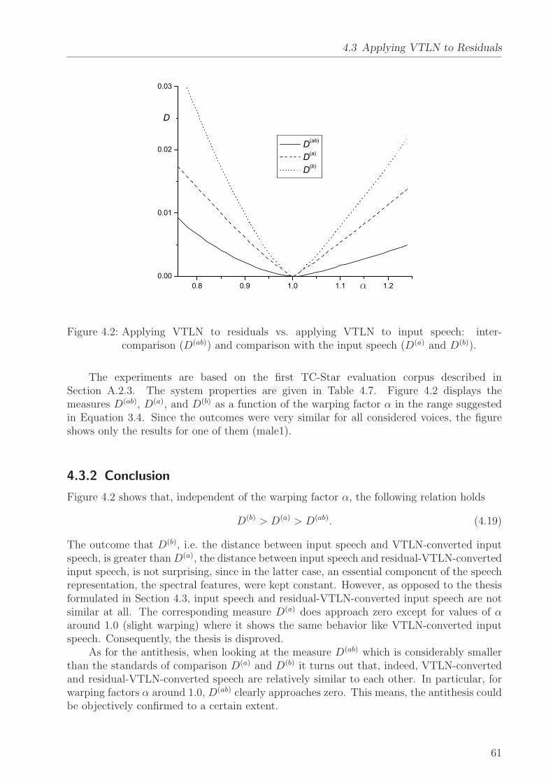
4.3 Applying VTLN to Residuals
0.8 0.9 1.0 1.1 1.20.00
0.01
0.02
0.03
D
D(ab)
D(a)
D(b)
. α
Figure 4.2: Applying VTLN to residuals vs. applying VTLN to input speech: inter-comparison (D(ab)) and comparison with the input speech (D(a) and D(b)).
The experiments are based on the first TC-Star evaluation corpus described inSection A.2.3. The system properties are given in Table 4.7. Figure 4.2 displays themeasures D(ab), D(a), and D(b) as a function of the warping factor α in the range suggestedin Equation 3.4. Since the outcomes were very similar for all considered voices, the figureshows only the results for one of them (male1).
4.3.2 Conclusion
Figure 4.2 shows that, independent of the warping factor α, the following relation holds
D(b) > D(a) > D(ab). (4.19)
The outcome that D(b), i.e. the distance between input speech and VTLN-converted inputspeech, is greater thanD(a), the distance between input speech and residual-VTLN-convertedinput speech, is not surprising, since in the latter case, an essential component of the speechrepresentation, the spectral features, were kept constant. However, as opposed to the thesisformulated in Section 4.3, input speech and residual-VTLN-converted input speech are notsimilar at all. The corresponding measure D(a) does approach zero except for values of αaround 1.0 (slight warping) where it shows the same behavior like VTLN-converted inputspeech. Consequently, the thesis is disproved.
As for the antithesis, when looking at the measure D(ab) which is considerably smallerthan the standards of comparison D(a) and D(b) it turns out that, indeed, VTLN-convertedand residual-VTLN-converted speech are relatively similar to each other. In particular, forwarping factors α around 1.0, D(ab) clearly approaches zero. This means, the antithesis couldbe objectively confirmed to a certain extent.
61
4 Residual Prediction
So, what is wrong with the two contradictions given in Section 4.3?
1. The source-filter model assumes that the excitation (represented by the residual) iswhite, i.e., it has a flat magnitude spectrum (cf. Section 2.4.3). In this case, anapplication of VTLN would not change the residual magnitude spectrum, and themagnitude spectra of input speech and residual-VTLN-converted input speech wereidentical. In the real world, however, the residuals are not white. They contain aconsiderable amount of spectral fine structure which is affected by both the applicationof VTLN to the residuals and to the input speech itself.
2. The realization that a linear transformation in feature space already includes the effectsof VTLN is of interest in speech recognition research that mostly does not look atthe residuals at all. But again, since the residuals carry a lot of voice-dependentinformation not covered by the features, the aforementioned equivalence does not applyto a voice conversion algorithm that processes the residuals by means of VTLN andthe features by means of linear transformation.
62
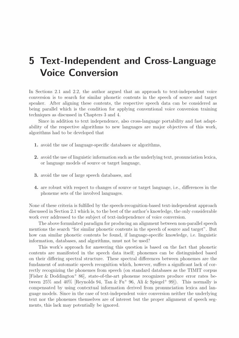
5 Text-Independent and Cross-Language
Voice Conversion
In Sections 2.1 and 2.2, the author argued that an approach to text-independent voiceconversion is to search for similar phonetic contents in the speech of source and targetspeaker. After aligning these contents, the respective speech data can be considered asbeing parallel which is the condition for applying conventional voice conversion trainingtechniques as discussed in Chapters 3 and 4.
Since in addition to text independence, also cross-language portability and fast adapt-ability of the respective algorithms to new languages are major objectives of this work,algorithms had to be developed that
1. avoid the use of language-specific databases or algorithms,
2. avoid the use of linguistic information such as the underlying text, pronunciation lexica,or language models of source or target language,
3. avoid the use of large speech databases, and
4. are robust with respect to changes of source or target language, i.e., differences in thephoneme sets of the involved languages.
None of these criteria is fulfilled by the speech-recognition-based text-independent approachdiscussed in Section 2.1 which is, to the best of the author’s knowledge, the only considerablework ever addressed to the subject of text-independence of voice conversion.
The above formulated paradigm for producing an alignment between non-parallel speechmentions the search “for similar phonetic contents in the speech of source and target”. Buthow can similar phonetic contents be found, if language-specific knowledge, i.e. linguisticinformation, databases, and algorithms, must not be used?
This work’s approach for answering this question is based on the fact that phoneticcontents are manifested in the speech data itself; phonemes can be distinguished basedon their differing spectral structure. These spectral differences between phonemes are thefundament of automatic speech recognition which, however, suffers a significant lack of cor-rectly recognizing the phonemes from speech (on standard databases as the TIMIT corpus[Fisher & Doddington+ 86], state-of-the-art phoneme recognizers produce error rates be-tween 25% and 40% [Reynolds 94, Tan & Fu+ 96, Ali & Spiegel+ 99]). This normally iscompensated by using contextual information derived from pronunciation lexica and lan-guage models. Since in the case of text-independent voice conversion neither the underlyingtext nor the phonemes themselves are of interest but the proper alignment of speech seg-ments, this lack may potentially be ignored.
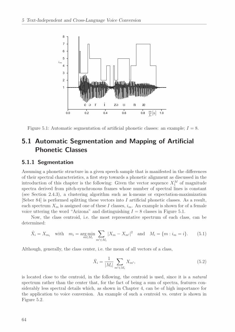
5 Text-Independent and Cross-Language Voice Conversion
0.0 0.2 0.4 0.6 0.8 1.0
0
1
2
3
4
5
6
7
k S
t/s
e @ r i z@ U n æ
1
8
7
6
5
4
3
2
1
. mfs
[s]
. im
Figure 5.1: Automatic segmentation of artificial phonetic classes: an example; I = 8.
5.1 Automatic Segmentation and Mapping of Artificial
Phonetic Classes
5.1.1 Segmentation
Assuming a phonetic structure in a given speech sample that is manifested in the differencesof their spectral characteristics, a first step towards a phonetic alignment as discussed in theintroduction of this chapter is the following: Given the vector sequence XM
1 of magnitudespectra derived from pitch-synchronous frames whose number of spectral lines is constant(see Section 2.4.3), a clustering algorithm such as k-means or expectation-maximization[Seber 84] is performed splitting these vectors into I artificial phonetic classes. As a result,each spectrum Xm is assigned one of these I classes, im. An example is shown for of a femalevoice uttering the word “Arizona” and distinguishing I = 8 classes in Figure 5.1.
Now, the class centroid, i.e. the most representative spectrum of each class, can bedetermined:
Xi = Xmiwith mi = arg min
m∈Mi
∑
m′∈Mi
|Xm −Xm′ |2 and Mi = {m : im = i}. (5.1)
Although, generally, the class center, i.e. the mean of all vectors of a class,
Xi =1
|Mi|∑
m′∈Mi
Xm′ , (5.2)
is located close to the centroid, in the following, the centroid is used, since it is a natural
spectrum rather than the center that, for the fact of being a sum of spectra, features con-siderably less spectral details which, as shown in Chapter 4, can be of high importance forthe application to voice conversion. An example of such a centroid vs. center is shown inFigure 5.2.
64
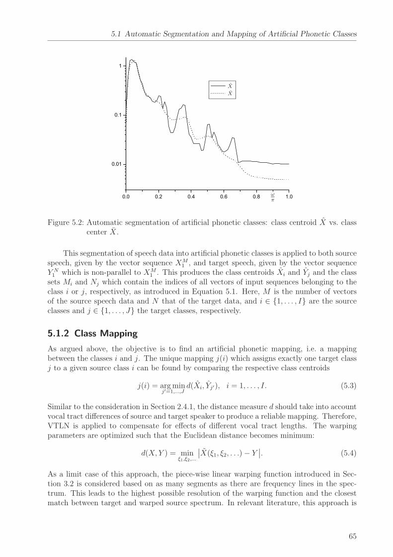
5.1 Automatic Segmentation and Mapping of Artificial Phonetic Classes
0.0 0.2 0.4 0.6 0.8 1.0
0.01
0.1
1
. ωπ
. X(ω)
. X
. X
Figure 5.2: Automatic segmentation of artificial phonetic classes: class centroid X vs. classcenter X.
This segmentation of speech data into artificial phonetic classes is applied to both sourcespeech, given by the vector sequence XM
1 , and target speech, given by the vector sequenceY N
1 which is non-parallel to XM1 . This produces the class centroids Xi and Yj and the class
sets Mi and Nj which contain the indices of all vectors of input sequences belonging to theclass i or j, respectively, as introduced in Equation 5.1. Here, M is the number of vectorsof the source speech data and N that of the target data, and i ∈ {1, . . . , I} are the sourceclasses and j ∈ {1, . . . , J} the target classes, respectively.
5.1.2 Class Mapping
As argued above, the objective is to find an artificial phonetic mapping, i.e. a mappingbetween the classes i and j. The unique mapping j(i) which assigns exactly one target classj to a given source class i can be found by comparing the respective class centroids
j(i) = arg minj′=1,...,J
d(Xi, Yj′), i = 1, . . . , I. (5.3)
Similar to the consideration in Section 2.4.1, the distance measure d should take into accountvocal tract differences of source and target speaker to produce a reliable mapping. Therefore,VTLN is applied to compensate for effects of different vocal tract lengths. The warpingparameters are optimized such that the Euclidean distance becomes minimum:
d(X,Y ) = minξ1,ξ2,...
∣
∣X(ξ1, ξ2, . . .) − Y∣
∣. (5.4)
As a limit case of this approach, the piece-wise linear warping function introduced in Sec-tion 3.2 is considered based on as many segments as there are frequency lines in the spec-trum. This leads to the highest possible resolution of the warping function and the closestmatch between target and warped source spectrum. In relevant literature, this approach is
65
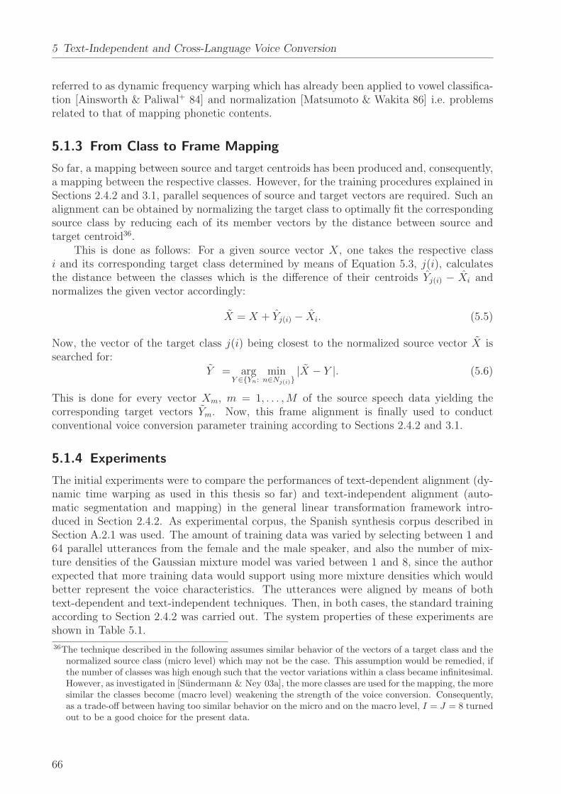
5 Text-Independent and Cross-Language Voice Conversion
referred to as dynamic frequency warping which has already been applied to vowel classifica-tion [Ainsworth & Paliwal+ 84] and normalization [Matsumoto & Wakita 86] i.e. problemsrelated to that of mapping phonetic contents.
5.1.3 From Class to Frame Mapping
So far, a mapping between source and target centroids has been produced and, consequently,a mapping between the respective classes. However, for the training procedures explained inSections 2.4.2 and 3.1, parallel sequences of source and target vectors are required. Such analignment can be obtained by normalizing the target class to optimally fit the correspondingsource class by reducing each of its member vectors by the distance between source andtarget centroid36.
This is done as follows: For a given source vector X, one takes the respective classi and its corresponding target class determined by means of Equation 5.3, j(i), calculatesthe distance between the classes which is the difference of their centroids Yj(i) − Xi andnormalizes the given vector accordingly:
X = X + Yj(i) − Xi. (5.5)
Now, the vector of the target class j(i) being closest to the normalized source vector X issearched for:
Y = arg minY ∈{Yn: n∈Nj(i)}
|X − Y |. (5.6)
This is done for every vector Xm, m = 1, . . . ,M of the source speech data yielding thecorresponding target vectors Ym. Now, this frame alignment is finally used to conductconventional voice conversion parameter training according to Sections 2.4.2 and 3.1.
5.1.4 Experiments
The initial experiments were to compare the performances of text-dependent alignment (dy-namic time warping as used in this thesis so far) and text-independent alignment (auto-matic segmentation and mapping) in the general linear transformation framework intro-duced in Section 2.4.2. As experimental corpus, the Spanish synthesis corpus described inSection A.2.1 was used. The amount of training data was varied by selecting between 1 and64 parallel utterances from the female and the male speaker, and also the number of mix-ture densities of the Gaussian mixture model was varied between 1 and 8, since the authorexpected that more training data would support using more mixture densities which wouldbetter represent the voice characteristics. The utterances were aligned by means of bothtext-dependent and text-independent techniques. Then, in both cases, the standard trainingaccording to Section 2.4.2 was carried out. The system properties of these experiments areshown in Table 5.1.
36The technique described in the following assumes similar behavior of the vectors of a target class and thenormalized source class (micro level) which may not be the case. This assumption would be remedied, ifthe number of classes was high enough such that the vector variations within a class became infinitesimal.However, as investigated in [Sundermann & Ney 03a], the more classes are used for the mapping, the moresimilar the classes become (macro level) weakening the strength of the voice conversion. Consequently,as a trade-off between having too similar behavior on the micro and on the macro level, I = J = 8 turnedout to be a good choice for the present data.
66
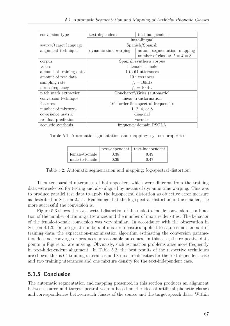
5.1 Automatic Segmentation and Mapping of Artificial Phonetic Classes
conversion type text-dependent text-independentintra-lingual
source/target language Spanish/Spanish
alignment technique dynamic time warping autom. segmentation, mappingnumber of classes: I = J = 8
corpus Spanish synthesis corpusvoices 1 female, 1 maleamount of training data 1 to 64 utterancesamount of test data 10 utterances
sampling rate fs = 16kHznorm frequency fn = 100Hz
pitch mark extraction Goncharoff/Gries (automatic)
conversion technique linear transformationfeatures 16th order line spectral frequenciesnumber of mixtures 1, 2, 4, or 8covariance matrix diagonal
residual prediction vocoder
acoustic synthesis frequency domain PSOLA
Table 5.1: Automatic segmentation and mapping: system properties.
text-dependent text-independent
female-to-male 0.38 0.49male-to-female 0.39 0.47
Table 5.2: Automatic segmentation and mapping: log-spectral distortion.
Then ten parallel utterances of both speakers which were different from the trainingdata were selected for testing and also aligned by means of dynamic time warping. This wasto produce parallel test data to apply the log-spectral distortion as objective error measureas described in Section 2.5.1. Remember that the log-spectral distortion is the smaller, themore successful the conversion is.
Figure 5.3 shows the log-spectral distortion of the male-to-female conversion as a func-tion of the number of training utterances and the number of mixture densities. The behaviorof the female-to-male conversion was very similar. In accordance with the observation inSection 4.1.3, for too great numbers of mixture densities applied to a too small amount oftraining data, the expectation-maximization algorithm estimating the conversion parame-ters does not converge or produces unreasonable outcomes. In this case, the respective datapoints in Figure 5.3 are missing. Obviously, such estimation problems arise more frequentlyin text-independent alignment. In Table 5.2, the best results of the respective techniquesare shown, this is 64 training utterances and 8 mixture densities for the text-dependent caseand two training utterances and one mixture density for the text-independent case.
5.1.5 Conclusion
The automatic segmentation and mapping presented in this section produces an alignmentbetween source and target spectral vectors based on the idea of artificial phonetic classesand correspondences between such classes of the source and the target speech data. Within
67
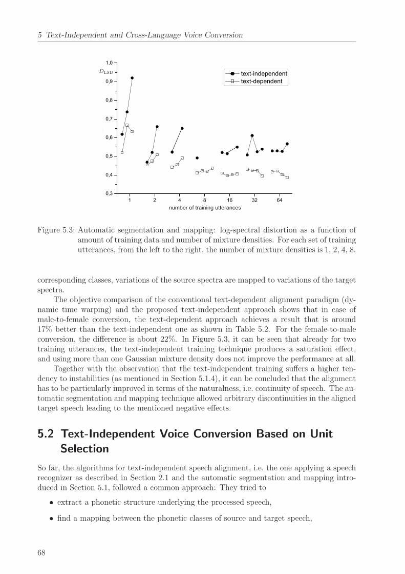
5 Text-Independent and Cross-Language Voice Conversion
1 2 4 8 16 32 640,3
0,4
0,5
0,6
0,7
0,8
0,9
1,0
DK
ain
training sentences
text-independent text-dependent
number of training utterances
. DLSD
Figure 5.3: Automatic segmentation and mapping: log-spectral distortion as a function ofamount of training data and number of mixture densities. For each set of trainingutterances, from the left to the right, the number of mixture densities is 1, 2, 4, 8.
corresponding classes, variations of the source spectra are mapped to variations of the targetspectra.
The objective comparison of the conventional text-dependent alignment paradigm (dy-namic time warping) and the proposed text-independent approach shows that in case ofmale-to-female conversion, the text-dependent approach achieves a result that is around17% better than the text-independent one as shown in Table 5.2. For the female-to-maleconversion, the difference is about 22%. In Figure 5.3, it can be seen that already for twotraining utterances, the text-independent training technique produces a saturation effect,and using more than one Gaussian mixture density does not improve the performance at all.
Together with the observation that the text-independent training suffers a higher ten-dency to instabilities (as mentioned in Section 5.1.4), it can be concluded that the alignmenthas to be particularly improved in terms of the naturalness, i.e. continuity of speech. The au-tomatic segmentation and mapping technique allowed arbitrary discontinuities in the alignedtarget speech leading to the mentioned negative effects.
5.2 Text-Independent Voice Conversion Based on Unit
Selection
So far, the algorithms for text-independent speech alignment, i.e. the one applying a speechrecognizer as described in Section 2.1 and the automatic segmentation and mapping intro-duced in Section 5.1, followed a common approach: They tried to
• extract a phonetic structure underlying the processed speech,
• find a mapping between the phonetic classes of source and target speech,
68
5.2 Text-Independent Voice Conversion Based on Unit Selection
• and transform the class mapping back to frame mapping.
All these steps may produce errors that accumulate and may lead to a poor parameterestimation or even to a convergence failure of the parameter estimation algorithm as reportedin Section 5.1.4. Hence, it would be helpful to avoid the detour through the class layer and,instead, find the mapping only using frame-based features.
Given the source speech feature sequence xM1 , one would straightforwardly be able to
determine the best-fitting sequence of corresponding target feature vectors yM1 by select-
ing from an arbitrary target feature sequence yN1 . This could be done by minimizing the
Euclidean distance between the compared feature vectors37:
ym = arg miny∈{y1,...,yN}
|xm − y|, m = 1, . . . ,M. (5.7)
However, as concluded in Section 5.1.5, there is a lack as for the continuity of the alignedtarget speech which has to be improved by taking into account also the frame context.Equation 5.7 ignores the context, since it determines the target feature vector ym just lookingat the corresponding source feature vector xm. Now, also distances to the neighbor vectorsym−1 and ym+1 are to be considered to improve continuity. This is done by once again usingthe unit selection framework introduced in Section 4.2.
To avoid the detour via the underlying phonetic structure, the base unit length is setto be a single frame. Interestingly, this time, both target and concatenation cost are com-puted in feature space as opposed to the application of unit selection to residual prediction,discussed in Section 4.2. There, the target costs were computed in feature space, whereasthe concatenation costs were computed in residual space. Consequently, in the case of unit-selection-based speech alignment, the feature vectors can be interpreted directly as databaseunits, i.e. t := x and u := y.
For determining the target vector sequence yM1 best-fitting a given source sequence xM
1 ,the sum of the target and concatenation costs applied to an arbitrarily selected sequenceof vectors taken from the non-parallel target sequence yN
1 has to be minimized. Since allcompared units are of the same structure (they are feature vectors) and dimensionality, thecost functions may be represented by Euclidean distances finally yielding
yM1 = arg min
yM1
M∑
m=1
{
w|ym − xm|2 + (1 − w)|ym−1 − ym|2}
. (5.8)
Here, the parameter w is for adjusting the tradeoff between fitting accuracy of source andtarget sequence and the spectral continuity criterion. As opposed to residual prediction basedon unit selection, this time, fundamental frequency and energy are not taken into account,since they do not directly influence the feature vectors. Finally, only the feature vectorsare used for the training of the linear-transformation-based conversion function ignoringfundamental frequency and energy. Consequently, their contribution weights (w1 and w2
according to Equation 4.8) are set to zero and w := w1. The weight w is determined byconducting informal listening tests; the author found that a rather reliable setting is w = 0.3(for the dependence of w on the amount of training data, see the discussion on the speechalignment paradox in Section 5.4.3).
37As opposed to Equation 5.3, this time, no VTLN is applied, since this would result in severe computationalproblems. Even without VTLN, the algorithm described in the following faces real-time factors greaterthan 100 as pointed out in Section 5.2.1. Nonetheless, the presented technique is rather robust againstvocal tract differences as the experimental results of Section 5.2.2 show.
69
5 Text-Independent and Cross-Language Voice Conversion
5.2.1 Time Behavior
As already discussed in Section 4.2.2, unit selection using single speech frames as base unitturns out to be very time-consuming. The structure of Equation 5.8 allows for applying dy-namic programming making the problem tractable. However, unlike well-known applicationsof dynamic programming (e.g. to dynamic time warping), in the case of unit selection-basedspeech alignment the search space is considerably larger: Conventionally, in the former case,the possible successors of a feature vector yn are limited to the set {yn, yn+1, yn+2}, whereasin the latter case all vectors are allowed. This leads to a time complexity of O(M ·N2).
Let us consider an example: For the male-to-female conversion described in Section 5.2.2,about 80s speech data of both source and target speaker was used. Taking into account thedifferent fundamental frequencies of the speakers (or rather: their different frame lengths),this resulted in M = 11400 and N = 16800 vectors. According to the above complexity, theexpression in the curly braces of Equation 5.8 had to be computed about 3.2 · 1012 times.After performing some of the steps discussed in Section 4.2.2 to reduce the complexity, thecomputation still took more than 3 hours on a 3GHz Intel Xeon processor corresponding toa real-time factor of about 150. It should, however, be mentioned that in several applica-tions of voice conversion, the training can be performed offline accepting real-time factorsabove 1.0. The unit selection can also be parallelized which allows for further acceleratingthe computation.
5.2.2 Experiments
The following experiments were to compare text-dependent voice conversion using dynamictime warping with the unit selection-based text-independent conversion. This was done byconducting subjective tests assessing both the voice similarity between converted and targetspeech and the overall speech quality of the conversion output. The experiments were basedon the first TC-Star evaluation corpus. From each of the 50 utterances, 10 utterances wererandomly selected to be used as test data.
For the text-independent case, the remaining 40 parallel utterances were randomly splityielding 20 different utterances for the source and for the target speaker, respectively, to havea real-world scenario where source and target texts are completely different. For the text-dependent case, 20 randomly selected parallel utterances were used for training. From thepossible twelve source/target speaker combinations, each gender combination was selectedonce.
In the test, 13 subjects (exclusively speech processing specialists) participated, the sys-tem properties are shown in Table 5.3. As a standard of comparison, the results werecompared to those produced in the first evaluation campaign of the project TC-Star (cf.Section A.1). Here, only the text-dependent data was evaluated. Both the assessed speechdata and the evaluation metrics were the same as in the present experiment. The numberof test subjects was 17. In addition to the text-dependent system according to Table 5.3, inthe TC-Star evaluation, another voice conversion system, in the following referred to as X,was evaluated.
As subjective error measures served mean opinion scores on both voice similarity andoverall speech quality as defined in Section 2.5.3. The outcomes of the experiments areshown in Table 5.4.
70
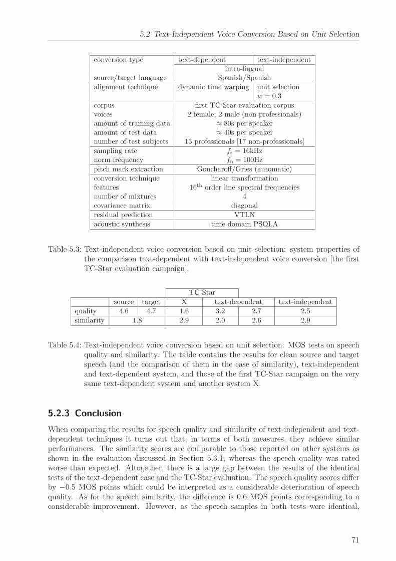
5.2 Text-Independent Voice Conversion Based on Unit Selection
conversion type text-dependent text-independentintra-lingual
source/target language Spanish/Spanish
alignment technique dynamic time warping unit selectionw = 0.3
corpus first TC-Star evaluation corpusvoices 2 female, 2 male (non-professionals)amount of training data ≈ 80s per speakeramount of test data ≈ 40s per speakernumber of test subjects 13 professionals [17 non-professionals]
sampling rate fs = 16kHznorm frequency fn = 100Hz
pitch mark extraction Goncharoff/Gries (automatic)
conversion technique linear transformationfeatures 16th order line spectral frequenciesnumber of mixtures 4covariance matrix diagonal
residual prediction VTLN
acoustic synthesis time domain PSOLA
Table 5.3: Text-independent voice conversion based on unit selection: system properties ofthe comparison text-dependent with text-independent voice conversion [the firstTC-Star evaluation campaign].
TC-Star
source target X text-dependent text-independent
quality 4.6 4.7 1.6 3.2 2.7 2.5
similarity 1.8 2.9 2.0 2.6 2.9
.............. .............. ..............
Table 5.4: Text-independent voice conversion based on unit selection: MOS tests on speechquality and similarity. The table contains the results for clean source and targetspeech (and the comparison of them in the case of similarity), text-independentand text-dependent system, and those of the first TC-Star campaign on the verysame text-dependent system and another system X.
5.2.3 Conclusion
When comparing the results for speech quality and similarity of text-independent and text-dependent techniques it turns out that, in terms of both measures, they achieve similarperformances. The similarity scores are comparable to those reported on other systems asshown in the evaluation discussed in Section 5.3.1, whereas the speech quality was ratedworse than expected. Altogether, there is a large gap between the results of the identicaltests of the text-dependent case and the TC-Star evaluation. The speech quality scores differby −0.5 MOS points which could be interpreted as a considerable deterioration of speechquality. As for the speech similarity, the difference is 0.6 MOS points corresponding to aconsiderable improvement. However, as the speech samples in both tests were identical,
71
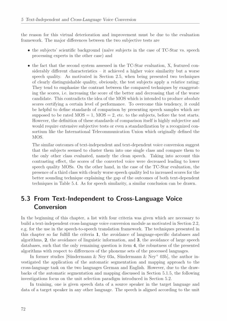
5 Text-Independent and Cross-Language Voice Conversion
the reason for this virtual deterioration and improvement must be due to the evaluationframework. The major differences between the two subjective tests are
• the subjects’ scientific background (naıve subjects in the case of TC-Star vs. speechprocessing experts in the other case) and
• the fact that the second system assessed in the TC-Star evaluation, X, featured con-siderably different characteristics – it achieved a higher voice similarity but a worsespeech quality. As motivated in Section 2.5, when being presented two techniquesof clearly distinguishable quality, obviously, the test subjects apply a relative rating:They tend to emphasize the contrast between the compared techniques by exaggerat-ing the scores, i.e. increasing the score of the better and decreasing that of the worsecandidate. This contradicts the idea of the MOS which is intended to produce absolute
scores certifying a certain level of performance. To overcome this tendency, it couldbe helpful to define standards of comparison by presenting speech samples which aresupposed to be rated MOS = 1, MOS = 2, etc. to the subjects, before the test starts.However, the definition of these standards of comparison itself is highly subjective andwould require extensive subjective tests or even a standardization by a recognized con-sortium like the International Telecommunication Union which originally defined theMOS.
The similar outcomes of text-independent and text-dependent voice conversion suggestthat the subjects seemed to cluster them into one single class and compare them tothe only other class evaluated, namely the clean speech. Taking into account thiscontrasting effect, the scores of the converted voice were decreased leading to lowerspeech quality MOSs. On the other hand, in the case of the TC-Star evaluation, thepresence of a third class with clearly worse speech quality led to increased scores for thebetter sounding technique explaining the gap of the outcomes of both text-dependenttechniques in Table 5.4. As for speech similarity, a similar conclusion can be drawn.
5.3 From Text-Independent to Cross-Language Voice
Conversion
In the beginning of this chapter, a list with four criteria was given which are necessary tobuild a text-independent cross-language voice conversion module as motivated in Section 2.2,e.g. for the use in the speech-to-speech translation framework. The techniques presented inthis chapter so far fulfill the criteria 1, the avoidance of language-specific databases andalgorithms, 2, the avoidance of linguistic information, and 3, the avoidance of large speechdatabases, such that the only remaining question is item 4, the robustness of the presentedalgorithms with respect to differences of the phoneme sets of the processed languages.
In former studies [Sundermann & Ney 03a, Sundermann & Ney+ 03b], the author in-vestigated the application of the automatic segmentation and mapping approach to thecross-language task on the two languages German and English. However, due to the draw-backs of the automatic segmentation and mapping discussed in Section 5.1.5, the followinginvestigations focus on the unit selection paradigm introduced in Section 5.2.
In training, one is given speech data of a source speaker in the target language anddata of a target speaker in any other language. The speech is aligned according to the unit
72
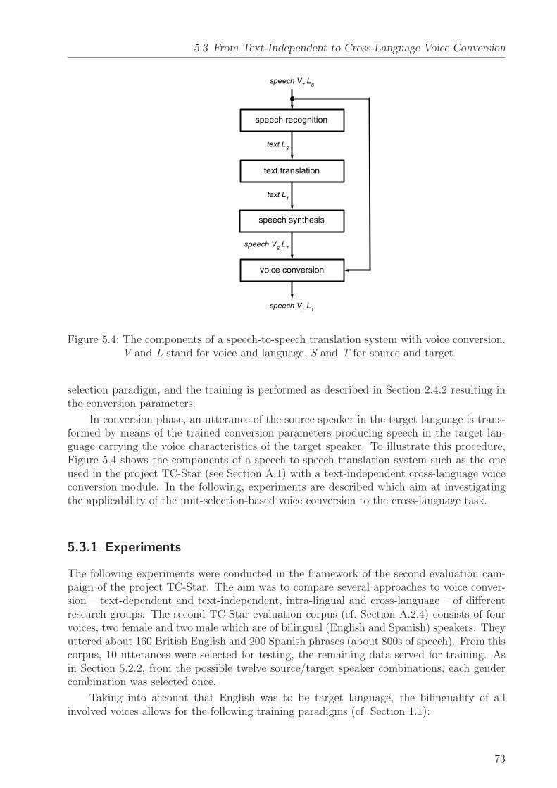
5.3 From Text-Independent to Cross-Language Voice Conversion
............
Figure 5.4: The components of a speech-to-speech translation system with voice conversion.V and L stand for voice and language, S and T for source and target.
selection paradigm, and the training is performed as described in Section 2.4.2 resulting inthe conversion parameters.
In conversion phase, an utterance of the source speaker in the target language is trans-formed by means of the trained conversion parameters producing speech in the target lan-guage carrying the voice characteristics of the target speaker. To illustrate this procedure,Figure 5.4 shows the components of a speech-to-speech translation system such as the oneused in the project TC-Star (see Section A.1) with a text-independent cross-language voiceconversion module. In the following, experiments are described which aim at investigatingthe applicability of the unit-selection-based voice conversion to the cross-language task.
5.3.1 Experiments
The following experiments were conducted in the framework of the second evaluation cam-paign of the project TC-Star. The aim was to compare several approaches to voice conver-sion – text-dependent and text-independent, intra-lingual and cross-language – of differentresearch groups. The second TC-Star evaluation corpus (cf. Section A.2.4) consists of fourvoices, two female and two male which are of bilingual (English and Spanish) speakers. Theyuttered about 160 British English and 200 Spanish phrases (about 800s of speech). From thiscorpus, 10 utterances were selected for testing, the remaining data served for training. Asin Section 5.2.2, from the possible twelve source/target speaker combinations, each gendercombination was selected once.
Taking into account that English was to be target language, the bilinguality of allinvolved voices allows for the following training paradigms (cf. Section 1.1):
73
5 Text-Independent and Cross-Language Voice Conversion
A. text-dependent intra-lingual – only English speech data is used for training
B. text-independent intra-lingual – only English speech data is used for training
C. text-dependent cross-language – the training is exclusively based on the Spanish speechdata of the involved speakers, but the conversion is applied to the English speech ofthe respective speakers (cf. the example discussed in Section 2.2)
D. text-independent cross-language – the training is based on the English speech of thesource speaker and the Spanish speech of the target speaker
The author submitted two systems, one based on paradigm A, the other based on D. Intotal, 9 systems participated in the evaluation.
To achieve the highest possible speech quality, the following changes were applied to thebaseline system of the first evaluation campaign discussed in Section 5.2.2:
• Pitch tracking. Correct and consistent pitch marks are crucial for a good acousticsynthesis based on time domain PSOLA. Also in training, pitch mark errors can leadto a poor estimation of the conversion parameters. Since recent studies on the reliabil-ity of pitch mark determination algorithms [Hoge & Kotnik+ 06, Kotnik & Hoge+ 06]showed that the pitch tracker used so far (Goncharoff/Gries) features a rather poorperformance, it was replaced by the Praat software [Boersma 01]. Additional Laryn-gograph data was used to achieve a high pitch marking accuracy. After automaticallydetermining the pitch marks, only those training speech files were selected for the pa-rameter training whose pitch marks could be reliably determined. This decision wasmade based on informal listening tests on the PSOLA-modified speech samples. Forthe test speech files where correct pitch marks are much more important some partswere manually corrected.
• Voicing information. According to the discussion in Section 3.1, only voiced speechportions were transformed, whereas unvoiced portions were generally copied to thetarget, or, in a few cases, slightly adapted by means of VTLN-based conversion.
• Feature dimensionality. According to the considerations in Section 2.4.2, due tothe low dimensionality of the processed feature vectors, spectral details are neglectedby the features which have to be reintroduced by residual prediction. Since the latterdecreases speech quality, it is preferable to use a higher dimensionality of the featurevector. On the other hand, one faces data sparseness leading to parameter estimationproblems when using too large dimensionalities. For the relatively large speech corpusavailable in the second TC-Star evaluation campaign, the dimensionality could beincreased to 32 without perceptively affecting speech quality.
• Voices. Finally, it is to be mentioned that the voices of the second TC-Star evaluationcorpus are of professional speakers as opposed to those of the first TC-Star evaluationcorpus. This fact can be of importance as experiences in speech synthesis researchshow [Black & Lenzo 03]. Professional speakers’ voices are more consistent and clearand tend to behave better when being automatically processed e.g. by means of a pitchtracker.
74
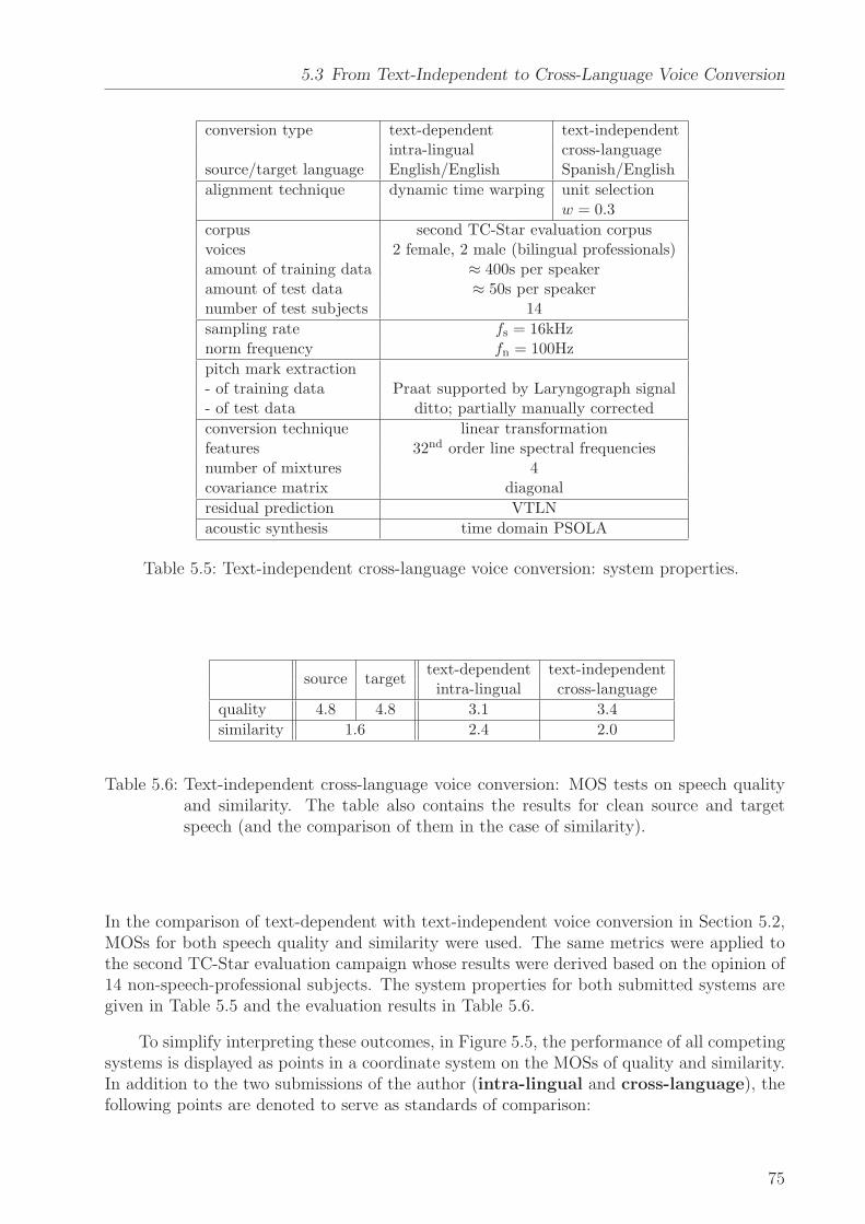
5.3 From Text-Independent to Cross-Language Voice Conversion
conversion type text-dependent text-independentintra-lingual cross-language
source/target language English/English Spanish/English
alignment technique dynamic time warping unit selectionw = 0.3
corpus second TC-Star evaluation corpusvoices 2 female, 2 male (bilingual professionals)amount of training data ≈ 400s per speakeramount of test data ≈ 50s per speakernumber of test subjects 14
sampling rate fs = 16kHznorm frequency fn = 100Hz
pitch mark extraction- of training data Praat supported by Laryngograph signal- of test data ditto; partially manually corrected
conversion technique linear transformationfeatures 32nd order line spectral frequenciesnumber of mixtures 4covariance matrix diagonal
residual prediction VTLN
acoustic synthesis time domain PSOLA
Table 5.5: Text-independent cross-language voice conversion: system properties.
text-dependent text-independentsource target
intra-lingual cross-language
quality 4.8 4.8 3.1 3.4
similarity 1.6 2.4 2.0
Table 5.6: Text-independent cross-language voice conversion: MOS tests on speech qualityand similarity. The table also contains the results for clean source and targetspeech (and the comparison of them in the case of similarity).
In the comparison of text-dependent with text-independent voice conversion in Section 5.2,MOSs for both speech quality and similarity were used. The same metrics were applied tothe second TC-Star evaluation campaign whose results were derived based on the opinion of14 non-speech-professional subjects. The system properties for both submitted systems aregiven in Table 5.5 and the evaluation results in Table 5.6.
To simplify interpreting these outcomes, in Figure 5.5, the performance of all competingsystems is displayed as points in a coordinate system on the MOSs of quality and similarity.In addition to the two submissions of the author (intra-lingual and cross-language), thefollowing points are denoted to serve as standards of comparison:
75
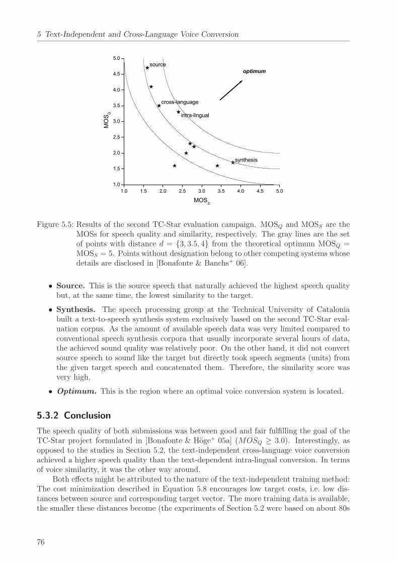
5 Text-Independent and Cross-Language Voice Conversion
Figure 5.5: Results of the second TC-Star evaluation campaign. MOSQ and MOSS are theMOSs for speech quality and similarity, respectively. The gray lines are the setof points with distance d = {3, 3.5, 4} from the theoretical optimum MOSQ =MOSS = 5. Points without designation belong to other competing systems whosedetails are disclosed in [Bonafonte & Banchs+ 06].
• Source. This is the source speech that naturally achieved the highest speech qualitybut, at the same time, the lowest similarity to the target.
• Synthesis. The speech processing group at the Technical University of Cataloniabuilt a text-to-speech synthesis system exclusively based on the second TC-Star eval-uation corpus. As the amount of available speech data was very limited compared toconventional speech synthesis corpora that usually incorporate several hours of data,the achieved sound quality was relatively poor. On the other hand, it did not convertsource speech to sound like the target but directly took speech segments (units) fromthe given target speech and concatenated them. Therefore, the similarity score wasvery high.
• Optimum. This is the region where an optimal voice conversion system is located.
5.3.2 Conclusion
The speech quality of both submissions was between good and fair fulfilling the goal of theTC-Star project formulated in [Bonafonte & Hoge+ 05a] (MOSQ ≥ 3.0). Interestingly, asopposed to the studies in Section 5.2, the text-independent cross-language voice conversionachieved a higher speech quality than the text-dependent intra-lingual conversion. In termsof voice similarity, it was the other way around.
Both effects might be attributed to the nature of the text-independent training method:The cost minimization described in Equation 5.8 encourages low target costs, i.e. low dis-tances between source and corresponding target vector. The more training data is available,the smaller these distances become (the experiments of Section 5.2 were based on about 80s
76
5.4 The Speech Alignment Paradox
of speech, whereas in the current case, it was around 400s). For an infinite amount of trainingdata, the author expected the distances to tend to zero or a relatively small limit. However,the more similar corresponding source and target vectors are, the less speaker-dependentinformation can be trained from them. For the limit case where source and target vectorsare equivalent one gets zero vectors and identity matrices as parameters of the linear trans-formation. In this case, the converted feature vectors are equivalent to the source vectors,i.e., one produces the source speech as output featuring the trivial baseline similarity but ahigh speech quality.
The described effect contradicts common experience in machine learning where theavailability of more training material usually allows for the extraction of more knowledge,i.e., in the aforementioned case, one would expect that more speaker-specific informationwould be trained. In the following section, this effect which the author refers to as speech
alignment paradox is investigated.Returning to the issue of robustness (item 4 of the list of criteria given at the very
beginning of this chapter), the outcomes of the experiments described in this section showthat both the text-dependent intra-lingual and the text-independent cross-language voiceconversion achieved similar results on the task investigated in the second TC-Star evalua-tion campaign. The frequently asked question, if the different phoneme sets of source andtarget language lead to parameter estimation problems, speech with audible accent, or signaldistortions, found a satisfying answer also in experiments on other languages as for instanceMedieval German or Chinese which the author conducted in the course of other projects.
Obviously, the search for similar feature vectors as performed by Equation 5.8 can alsobe successful even when the source vector comes from a phoneme that does not exist inthe target language. The algorithm straightforwardly selects the frame best resembling thesource frame, independent of the phoneme it comes from. The more data is available, themore successful is this search, since the numerous phoneme transitions in the speech producea large variety of sounds not available in the standard phoneme set.
It has also to be taken into account that the linear transformation paradigm describedin Section 2.4.2 is applied to source vectors that come from canonical source speech. Thismeans, the baseline is not accented or distorted, and this also applies to the residuals, ifthey are predicted by means of the VTLN technique. Considering the small number ofGaussian mixtures (4 in this chapter’s experiments) suggests that the linear transformationis not completely phoneme-dependent but rather represents the speech characteristics byfour global classes. Hence, the transformation does not affect single phonemes but convertsthe voice characteristics in a more global way avoiding the aforementioned effects.
5.4 The Speech Alignment Paradox
In the previous section, it was found that when applying unit-selection-based speechalignment to the training of a voice conversion system one faces the following effect:
......The more training data is available, the less speaker-specific information is trained.
The author expected that in the limit case, i.e., when infinitely much data was avail-able source and aligned target speech would be identical such that the training wouldbe trivial. In this section, this effect, referred to as speech alignment paradox, is to beinvestigated by experimental and mathematical means.
77
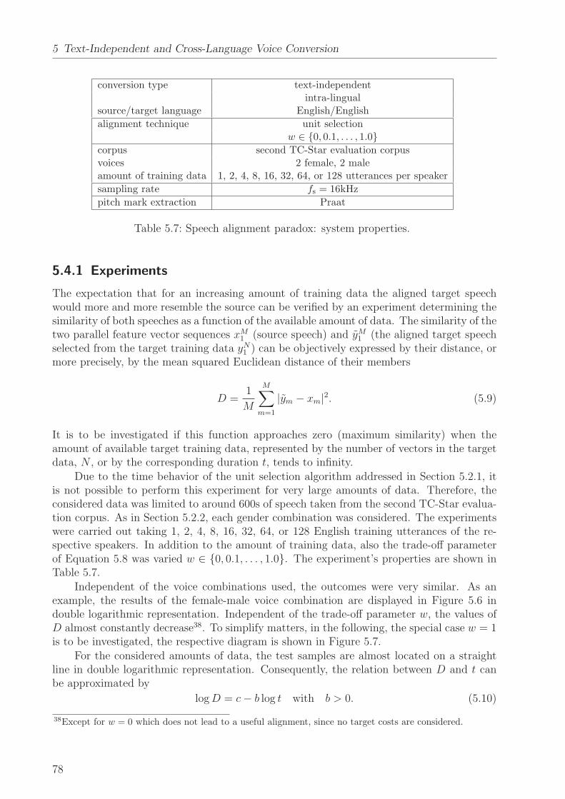
5 Text-Independent and Cross-Language Voice Conversion
conversion type text-independentintra-lingual
source/target language English/English
alignment technique unit selectionw ∈ {0, 0.1, . . . , 1.0}
corpus second TC-Star evaluation corpusvoices 2 female, 2 maleamount of training data 1, 2, 4, 8, 16, 32, 64, or 128 utterances per speaker
sampling rate fs = 16kHz
pitch mark extraction Praat
Table 5.7: Speech alignment paradox: system properties.
5.4.1 Experiments
The expectation that for an increasing amount of training data the aligned target speechwould more and more resemble the source can be verified by an experiment determining thesimilarity of both speeches as a function of the available amount of data. The similarity of thetwo parallel feature vector sequences xM
1 (source speech) and yM1 (the aligned target speech
selected from the target training data yN1 ) can be objectively expressed by their distance, or
more precisely, by the mean squared Euclidean distance of their members
D =1
M
M∑
m=1
|ym − xm|2. (5.9)
It is to be investigated if this function approaches zero (maximum similarity) when theamount of available target training data, represented by the number of vectors in the targetdata, N , or by the corresponding duration t, tends to infinity.
Due to the time behavior of the unit selection algorithm addressed in Section 5.2.1, itis not possible to perform this experiment for very large amounts of data. Therefore, theconsidered data was limited to around 600s of speech taken from the second TC-Star evalua-tion corpus. As in Section 5.2.2, each gender combination was considered. The experimentswere carried out taking 1, 2, 4, 8, 16, 32, 64, or 128 English training utterances of the re-spective speakers. In addition to the amount of training data, also the trade-off parameterof Equation 5.8 was varied w ∈ {0, 0.1, . . . , 1.0}. The experiment’s properties are shown inTable 5.7.
Independent of the voice combinations used, the outcomes were very similar. As anexample, the results of the female-male voice combination are displayed in Figure 5.6 indouble logarithmic representation. Independent of the trade-off parameter w, the values ofD almost constantly decrease38. To simplify matters, in the following, the special case w = 1is to be investigated, the respective diagram is shown in Figure 5.7.
For the considered amounts of data, the test samples are almost located on a straightline in double logarithmic representation. Consequently, the relation between D and t canbe approximated by
logD = c− b log t with b > 0. (5.10)
38Except for w = 0 which does not lead to a useful alignment, since no target costs are considered.
78
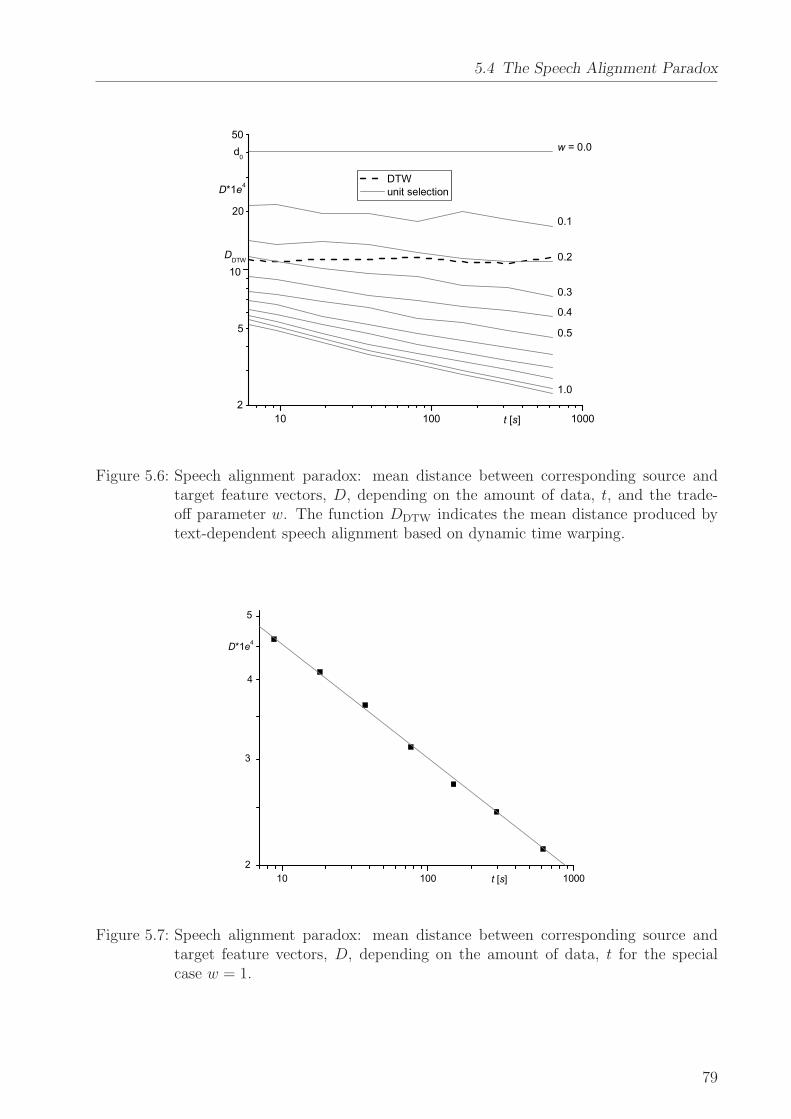
5.4 The Speech Alignment Paradox
Figure 5.6: Speech alignment paradox: mean distance between corresponding source andtarget feature vectors, D, depending on the amount of data, t, and the trade-off parameter w. The function DDTW indicates the mean distance produced bytext-dependent speech alignment based on dynamic time warping.
Figure 5.7: Speech alignment paradox: mean distance between corresponding source andtarget feature vectors, D, depending on the amount of data, t for the specialcase w = 1.
79
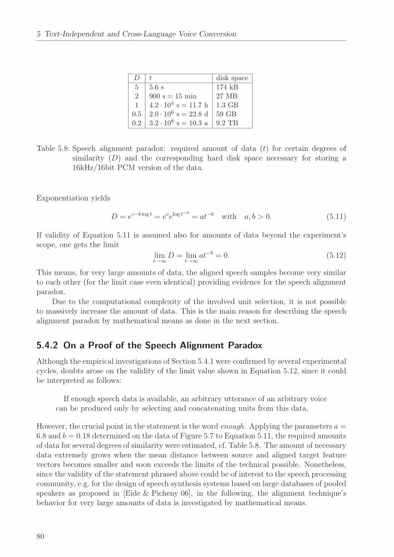
5 Text-Independent and Cross-Language Voice Conversion
D t disk space
5 5.6 s 174 kB2 900 s = 15 min 27 MB1 4.2 · 104 s = 11.7 h 1.3 GB
0.5 2.0 · 106 s = 22.8 d 59 GB0.2 3.2 · 108 s = 10.3 a 9.2 TB
Table 5.8: Speech alignment paradox: required amount of data (t) for certain degrees ofsimilarity (D) and the corresponding hard disk space necessary for storing a16kHz/16bit PCM version of the data.
Exponentiation yields
D = ec−b log t = ecelog t−b
= at−b with a, b > 0. (5.11)
If validity of Equation 5.11 is assumed also for amounts of data beyond the experiment’sscope, one gets the limit
limt→∞
D = limt→∞
at−b = 0. (5.12)
This means, for very large amounts of data, the aligned speech samples become very similarto each other (for the limit case even identical) providing evidence for the speech alignmentparadox.
Due to the computational complexity of the involved unit selection, it is not possibleto massively increase the amount of data. This is the main reason for describing the speechalignment paradox by mathematical means as done in the next section.
5.4.2 On a Proof of the Speech Alignment Paradox
Although the empirical investigations of Section 5.4.1 were confirmed by several experimentalcycles, doubts arose on the validity of the limit value shown in Equation 5.12, since it couldbe interpreted as follows:
If enough speech data is available, an arbitrary utterance of an arbitrary voicecan be produced only by selecting and concatenating units from this data.
However, the crucial point in the statement is the word enough. Applying the parameters a =6.8 and b = 0.18 determined on the data of Figure 5.7 to Equation 5.11, the required amountsof data for several degrees of similarity were estimated, cf. Table 5.8. The amount of necessarydata extremely grows when the mean distance between source and aligned target featurevectors becomes smaller and soon exceeds the limits of the technical possible. Nonetheless,since the validity of the statement phrased above could be of interest to the speech processingcommunity, e.g. for the design of speech synthesis systems based on large databases of pooledspeakers as proposed in [Eide & Picheny 06], in the following, the alignment technique’sbehavior for very large amounts of data is investigated by mathematical means.
80
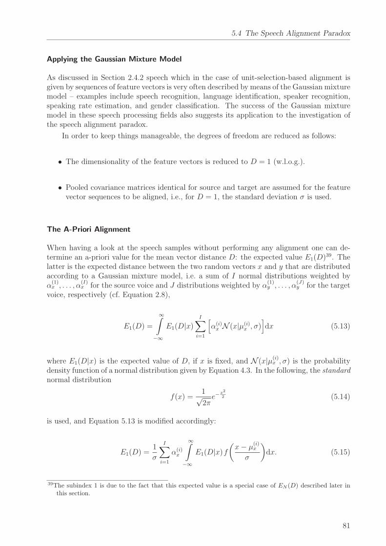
5.4 The Speech Alignment Paradox
Applying the Gaussian Mixture Model
As discussed in Section 2.4.2 speech which in the case of unit-selection-based alignment isgiven by sequences of feature vectors is very often described by means of the Gaussian mixturemodel – examples include speech recognition, language identification, speaker recognition,speaking rate estimation, and gender classification. The success of the Gaussian mixturemodel in these speech processing fields also suggests its application to the investigation ofthe speech alignment paradox.
In order to keep things manageable, the degrees of freedom are reduced as follows:
• The dimensionality of the feature vectors is reduced to D = 1 (w.l.o.g.).
• Pooled covariance matrices identical for source and target are assumed for the featurevector sequences to be aligned, i.e., for D = 1, the standard deviation σ is used.
The A-Priori Alignment
When having a look at the speech samples without performing any alignment one can de-termine an a-priori value for the mean vector distance D: the expected value E1(D)39. Thelatter is the expected distance between the two random vectors x and y that are distributedaccording to a Gaussian mixture model, i.e. a sum of I normal distributions weighted byα
(1)x , . . . , α
(I)x for the source voice and J distributions weighted by α
(1)y , . . . , α
(J)y for the target
voice, respectively (cf. Equation 2.8),
E1(D) =
∞∫
−∞
E1(D|x)I∑
i=1
[
α(i)x N (x|µ(i)
x , σ)]
dx (5.13)
where E1(D|x) is the expected value of D, if x is fixed, and N (x|µ(i)x , σ) is the probability
density function of a normal distribution given by Equation 4.3. In the following, the standard
normal distribution
f(x) =1√2πe−
x2
2 (5.14)
is used, and Equation 5.13 is modified accordingly:
E1(D) =1
σ
I∑
i=1
α(i)x
∞∫
−∞
E1(D|x)f(
x− µ(i)x
σ
)
dx. (5.15)
39The subindex 1 is due to the fact that this expected value is a special case of EN (D) described later inthis section.
81
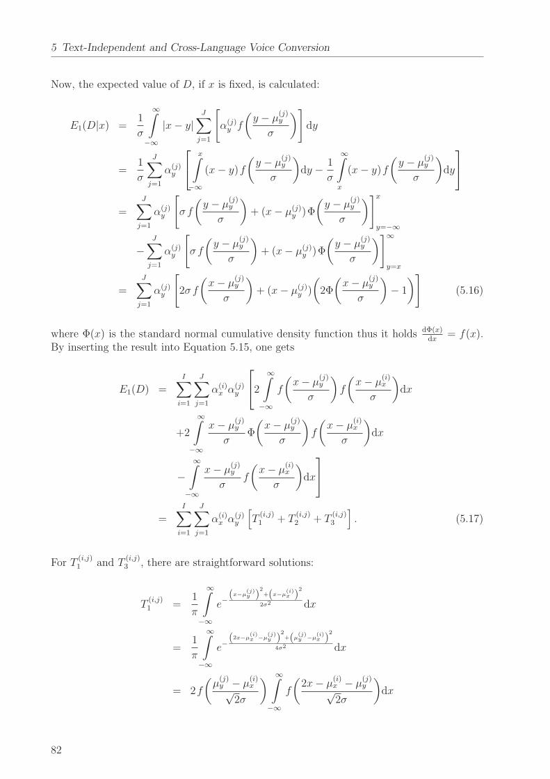
5 Text-Independent and Cross-Language Voice Conversion
Now, the expected value of D, if x is fixed, is calculated:
E1(D|x) =1
σ
∞∫
−∞
|x− y|J∑
j=1
[
α(j)y f
(
y − µ(j)y
σ
)
]
dy
=1
σ
J∑
j=1
α(j)y
x∫
−∞
(x− y)f
(
y − µ(j)y
σ
)
dy − 1
σ
∞∫
x
(x− y)f
(
y − µ(j)y
σ
)
dy
=J∑
j=1
α(j)y
[
σf
(
y − µ(j)y
σ
)
+ (x− µ(j)y )Φ
(
y − µ(j)y
σ
)
]x
y=−∞
= −J∑
j=1
α(j)y
[
σf
(
y − µ(j)y
σ
)
+ (x− µ(j)y )Φ
(
y − µ(j)y
σ
)
]∞
y=x
=J∑
j=1
α(j)y
[
2σf
(
x− µ(j)y
σ
)
+ (x− µ(j)y )
(
2Φ
(
x− µ(j)y
σ
)
− 1
)
]
(5.16)
where Φ(x) is the standard normal cumulative density function thus it holds dΦ(x)dx
= f(x).By inserting the result into Equation 5.15, one gets
E1(D) =I∑
i=1
J∑
j=1
α(i)x α
(j)y
2
∞∫
−∞
f
(
x− µ(j)y
σ
)
f
(
x− µ(i)x
σ
)
dx
+2
∞∫
−∞
x− µ(j)y
σΦ
(
x− µ(j)y
σ
)
f
(
x− µ(i)x
σ
)
dx
−∞∫
−∞
x− µ(j)y
σf
(
x− µ(i)x
σ
)
dx
=I∑
i=1
J∑
j=1
α(i)x α
(j)y
[
T(i,j)1 + T
(i,j)2 + T
(i,j)3
]
. (5.17)
For T(i,j)1 and T
(i,j)3 , there are straightforward solutions:
T(i,j)1 =
1
π
∞∫
−∞
e−(x−µ
(j)y )
2+(x−µ
(i)x )
2
2σ2 dx
=1
π
∞∫
−∞
e−(2x−µ
(i)x −µ
(j)y )
2+(µ
(j)y −µ
(i)x )
2
4σ2 dx
= 2f
(
µ(j)y − µ
(i)x√
2σ
)
∞∫
−∞
f
(
2x− µ(i)x − µ
(j)y√
2σ
)
dx
82
5.4 The Speech Alignment Paradox
T(i,)1 = 2f
(
µ(j)y − µ
(i)x√
2σ
)
[
σ√2
Φ
(
2x− µ(i)x − µ
(j)y√
2σ
)
]∞
x=−∞
=√
2σf
(
µ(j)y − µ
(i)x√
2σ
)
; (5.18)
T(i,j)3 =
[
(µ(i)x − µ(j)
y )Φ
(
x− µ(i)x
σ
)
− σf
(
x− µ(i)x
σ
)
]∞
x=−∞
= µ(j)y − µ(i)
x , (5.19)
whereas T(i,j)2 requires a more complex derivation given in Section A.3.4:
T(i,j)2 =
√2σf
(
µ(j)y − µ
(i)x√
2σ
)
+ 2(µ(j)y − µ(i)
x )
[
Φ
(
µ(j)y − µ
(i)x√
2σ
)
− 1
]
(5.20)
yielding the requested expected value of D (in the following, the variable δ(i,j) = µ(j)y − µ
(i)x ,
the difference between the means of the ith source density and the jth target density, is used):
E1(D) =I∑
i=1
J∑
j=1
α(i)x α
(j)y
[
2√
2σf
(
δ(i,j)
√2σ
)
+ 2δ(i,j) Φ
(
δ(i,j)
√2σ
)
− δ(i,j)
]
. (5.21)
For some of the following considerations, the special case I = J = 1 is to be consideredwhere the quantity δ = δ(1,1) is used and Equation 5.21 becomes
E1(D) = 2√
2σf
(
δ√2σ
)
+ 2δΦ
(
δ√2σ
)
− δ. (5.22)
Figure 5.8 shows E1(D) as a function of δ for σ ∈ {0.5, 1, 2} and indicates the lower boundof E1(D) given by the limit
limδ/σ→±∞
E1(D) = |δ|. (5.23)
This limit can also be calculated using Equation 5.15: When δσ
approaches infinity thedeviation of x’s distribution function becomes infinitely small as compared with its mean’sdistance to y’s mean. Consequently, the normal distribution can be replaced by the Diracdelta function ∆ yielding
limδ/σ→±∞
E1(D) = limδ/σ→±∞
1
σ
∞∫
−∞
E1(D|x)f(
x− µx
σ
)
dx
= limδ/σ→±∞
1
σ
∞∫
−∞
E1(D|x)∆
(
x− µx
σ
)
dx
= limδ/σ→±∞
1
σ
∞∫
−∞
E1(D|σξ + µx)∆(ξ)σdξ
= limδ/σ→±∞
E1(D|µx) (5.24)
83

5 Text-Independent and Cross-Language Voice Conversion
. σ
. σ
. σ
. δ
. δ
Figure 5.8: Speech alignment paradox: expected value of the mean distance between twofeature vectors E1(D) as a function of the difference of the distribution means δand of the standard deviation σ.
Applying Equation 5.16 yields
lim..δ/σ→±∞
E1(D) = limδ/σ→±∞
2σf
(
δ
σ
)
+ δ
[
Φ
(
δ
σ
)
− 1
]
= |δ|. (5.25)
Incidentally, the author found that for the special case δ = 0 and σ = 1, Equation 5.21becomes the closed form solution of what in statistical process control is referred to as theconstant d2 (the expected distance between two instances of a standard normally distributedrandom process) whose value 1.1284 determined by numerical means is given in textbookson process control, e.g. [Montgomery 96]:
d2 =2√π. (5.26)
Towards a Closed Form Solution
After studying the a-priori alignment, the above approach is to be extended to the unitselection-based alignment considering several mixture densities. The principal difference tothe former is the minimization in Equation 5.8 to search for the optimal sequence of vectors.This directly affects the expected value of D given x (cf. Equation 5.16), since now theprobability density function of y is not a sum over normal distributions but over the morecomplicated terms pN(y|x, j):
EN(D|x) =
∞∫
−∞
|x− y|J∑
j=1
[
α(j)y pN(y|x, j)
]
dy. (5.27)
As mentioned earlier, N denotes the number of feature vectors in the target feature vectorsequence yN
1 serving as a pool appropriate units are selected from, see Section 5.2. Again, it
84
5.4 The Speech Alignment Paradox
is assumed that these vectors are distributed according to a Gaussian mixture model withJ mixtures and the parameters α
(j)y , µ
(j)y and σ are independent of each other.
Given a mixture j, for each possible y, the probability density of the nth target featurevector being equal to y and closest to x is calculated. The sum over all these vectors from1 to N yields the sought-after density pN(y|x, j).
In detail: The probability density of the nth vector being equal to y is
P (j)n =
1
σf
(
y − µ(j)y
σ
)
. (5.28)
The probability of the nth vector being closest to x means that the distance to all othervectors yν for ν ∈ {1, . . . , N}, ν 6= n is greater than that to yn or, given yn = y, that|yν − x| > |y − x|:
Q(j)n = p
(
N∧
ν=1
ν 6=n
|yν − x| > |y − x|)
=N∏
ν=1
ν 6=n
p(|yν − x| > |y − x|)
= p(|ψ − x| > |y − x|)N−1
=
{
p(ψ < y ∨ ψ > 2x− y)N−1 for y < x
p(ψ > y ∨ ψ < 2x− y)N−1 otherwise
=
(
Φ
(
y − µ(j)y
σ
)
+ 1 − Φ
(
2x− y − µ(j)y
σ
))N−1
for y < x
(
1 − Φ
(
y − µ(j)y
σ
)
+ Φ
(
2x− y − µ(j)y
σ
))N−1
otherwise
Here, ψ is a y-like distributed random variable replacing yν for ν ∈ {1, . . . , N}, ν 6= n.Accordingly, Equation 5.27 becomes (also cf. Equation 5.16)
EN(D|x) =J∑
j=1
α(j)y
∞∫
−∞
|x− y|N∑
n=1
(P (j)n Q(j)
n )dy (5.29)
=N
σ
J∑
j=1
α(j)y
x∫
−∞
(x−y)f(
y−µ(j)y
σ
)(
1+Φ
(
y−µ(j)y
σ
)
−Φ
(
2x−y−µ(j)y
σ
))N−1
dy
= −∞∫
x
(x− y)f
(
y − µ(j)y
σ
)(
1 − Φ
(
y − µ(j)y
σ
)
+ Φ
(
2x− y − µ(j)y
σ
))N−1
dy
.
85
5 Text-Independent and Cross-Language Voice Conversion
As already mentioned in Footnote 39, for N = 1, this becomes identical to Equation 5.16.One can show that Equation 5.29 can be simplified to the problem of solving
∫
fm(x) Φn(x− δ)dx for m ∈ {1, 2} and n ∈ {0, 1, 2, . . .} (5.30)
whose closed-form solution does not seem to exist for n > 1.However, if large values of δ
σare considered (cf. Equation 5.23), for the special case I = J = 1,
one gets a very exact approximation of the sought-after expected value of D as alreadydiscussed in Equation 5.24 by
limδ/σ→±∞
EN(D) = limδ/σ→±∞
EN(D|µx). (5.31)
Considering also Equation 5.29 where y is substituted by z + µx yields
limδ/σ→±∞
EN(D) = limδ/σ→±∞
N
σ
−0∫
−∞
z f
(
z − δ
σ
)(
1 + Φ
(
z − δ
σ
)
− Φ
(−z − δ
σ
))N−1
dz
+
∞∫
0
z f
(
z − δ
σ
)(
1 − Φ
(
z − δ
σ
)
+ Φ
(−z − δ
σ
))N−1
dz
. (5.32)
For δσ→ ∞, the first integral of this equation becomes zero, since
limδ/σ→∞
f
(
z − δ
σ
)
= 0 for z < 0. (5.33)
Moreover, for the remaining integral holds
limδ/σ→∞
Φ
(−z − δ
σ
)
= 0 for z > 0, (5.34)
and, taking into account Equation 5.33, the remaining integral’s lower limit can be extendedto −∞, since this adds zero. Consequently, for δ
σ→ ∞, Equation 5.32 can be expressed by
limδ/σ→∞
EN(D) = limδ/σ→∞
N
σ
∞∫
−∞
z f
(
z − δ
σ
)(
1 − Φ
(
z − δ
σ
))N−1
dz. (5.35)
Applying the above steps to the case δσ→ −∞ and using the relations Φ(x) = 1 − Φ(−x)
and f(x) = f(−x) yields
limδ/σ→±∞
EN(D) = limδ/σ→±∞
N
σ
∞∫
−∞
z f
(
z − |δ|σ
)(
1 − Φ
(
z − |δ|σ
))N−1
dz. (5.36)
86
5.4 The Speech Alignment Paradox
N µ(N) closed form of µ(N)
1 0 0
2 0.561√π
3 0.853
2√
π
4 1.036√π3
arctan√
2
5 1.1615√π3
arctan√
2 − 5
2√
π
10 1.54
100 2.51
1 000 3.24
1 000 000 4.86
Table 5.9: Speech alignment paradox: the offset constant µ(N) for different values of N .
Substituting z by |δ| − σξ and taking into account that the quotient δσ
disappears whichallows for removing the limit leads to
limδ/σ→±∞
EN(D) =N
σ
−∞∫
∞
(|δ| − σξ)f(−ξ) (1 − Φ(−ξ))N−1 (−σdξ)
= N
∞∫
−∞
(|δ| − σξ)f(ξ)Φ(ξ)N−1dξ
= N |δ|[
Φ(ξ)N
N
]∞
ξ=−∞− σN
∞∫
−∞
ξf(ξ)Φ(ξ)N−1dξ
= |δ| − σµ(N). (5.37)
The structure of this formula gives a qualitative overview about some of the expectedvalue’s characteristics. It consists of the term |δ| being independent of the standard deviationσ and a term which is a constant with respect to |δ| but linearly depends on σ.
[David & Nagaraja 03] give solutions to µ(N) for N ∈ {1, ..., 5}, but so far, for k > 5,the author did not succeed in finding a closed form. Table 5.9 gives some example values ofµ(N), and Figure 5.9 shows a plot of EN(D) as a function of δ for several values of N . Forlarge δ, the graphs approach |δ| − σµ(N) as derived in Equation 5.37, and for N = 1, oneobtains the special case discussed in Equations 5.23 and 5.25.
87
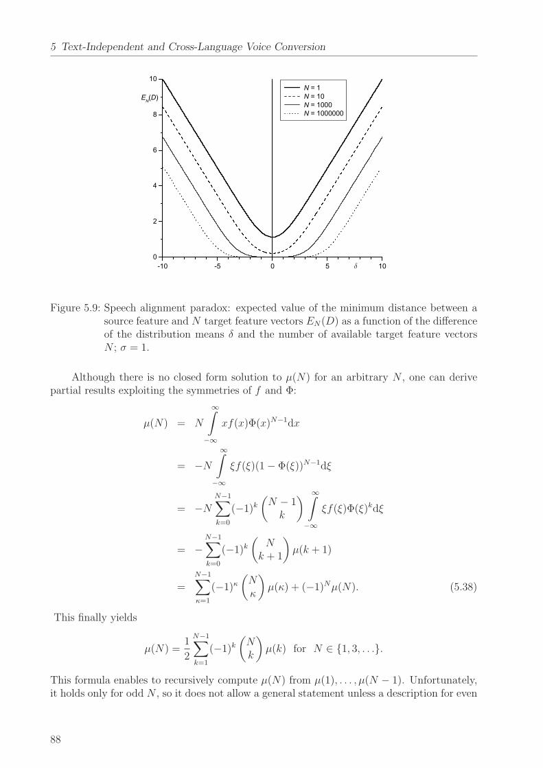
5 Text-Independent and Cross-Language Voice Conversion
. σ
. σ
. σ
. δ
. δ
Figure 5.9: Speech alignment paradox: expected value of the minimum distance between asource feature and N target feature vectors EN(D) as a function of the differenceof the distribution means δ and the number of available target feature vectorsN ; σ = 1.
Although there is no closed form solution to µ(N) for an arbitrary N , one can derivepartial results exploiting the symmetries of f and Φ:
µ(N) = N
∞∫
−∞
xf(x)Φ(x)N−1dx
= −N∞∫
−∞
ξf(ξ)(1 − Φ(ξ))N−1dξ
= −NN−1∑
k=0
(−1)k
(
N − 1k
)
∞∫
−∞
ξf(ξ)Φ(ξ)kdξ
= −N−1∑
k=0
(−1)k
(
Nk + 1
)
µ(k + 1)
=N−1∑
κ=1
(−1)κ
(
Nκ
)
µ(κ) + (−1)Nµ(N). (5.38)
This finally yields
µ(N) =1
2
N−1∑
k=1
(−1)k
(
Nk
)
µ(k) for N ∈ {1, 3, . . .}.
This formula enables to recursively compute µ(N) from µ(1), . . . , µ(N − 1). Unfortunately,it holds only for odd N , so it does not allow a general statement unless a description for even
88
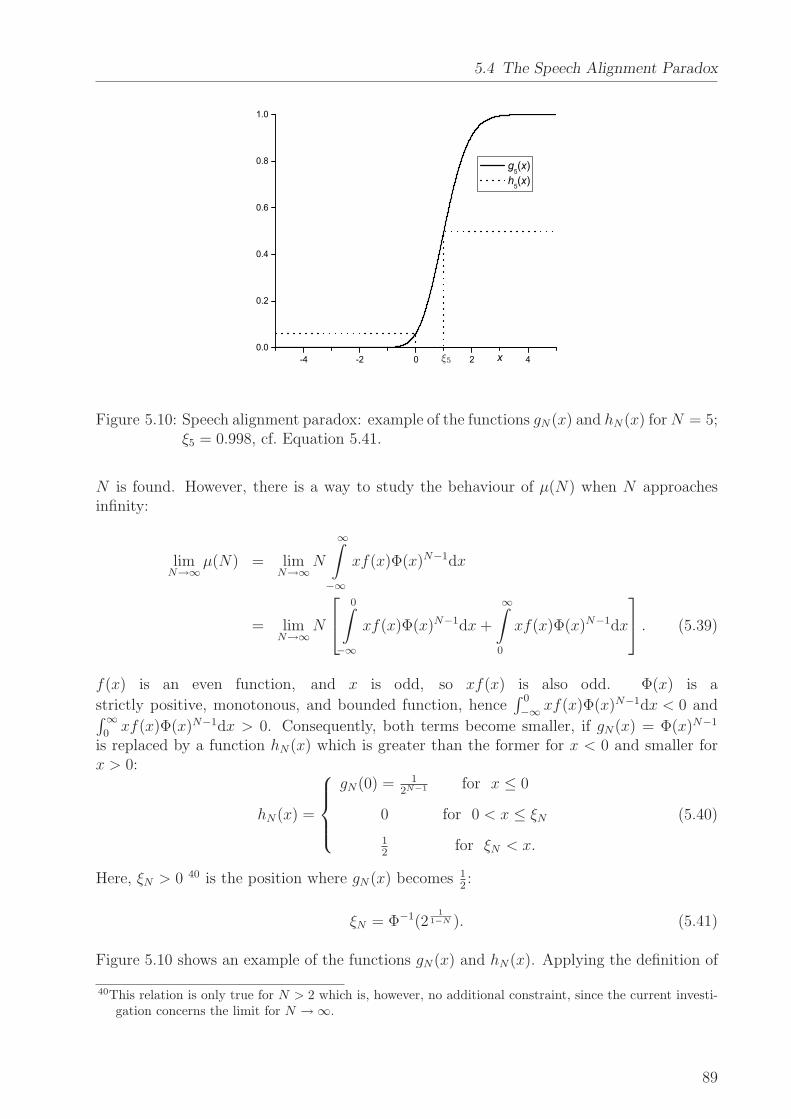
5.4 The Speech Alignment Paradox
. σ
. σ
. σ
. δ
. ξ5
Figure 5.10: Speech alignment paradox: example of the functions gN(x) and hN(x) forN = 5;ξ5 = 0.998, cf. Equation 5.41.
N is found. However, there is a way to study the behaviour of µ(N) when N approachesinfinity:
limN→∞
µ(N) = limN→∞
N
∞∫
−∞
xf(x)Φ(x)N−1dx
= limN→∞
N
0∫
−∞
xf(x)Φ(x)N−1dx+
∞∫
0
xf(x)Φ(x)N−1dx
. (5.39)
f(x) is an even function, and x is odd, so xf(x) is also odd. Φ(x) is a
strictly positive, monotonous, and bounded function, hence∫ 0
−∞ xf(x)Φ(x)N−1dx < 0 and∫∞0xf(x)Φ(x)N−1dx > 0. Consequently, both terms become smaller, if gN(x) = Φ(x)N−1
is replaced by a function hN(x) which is greater than the former for x < 0 and smaller forx > 0:
hN(x) =
gN(0) = 12N−1 for x ≤ 0
0 for 0 < x ≤ ξN
12
for ξN < x.
(5.40)
Here, ξN > 0 40 is the position where gN(x) becomes 12:
ξN = Φ−1(21
1−N ). (5.41)
Figure 5.10 shows an example of the functions gN(x) and hN(x). Applying the definition of
40This relation is only true for N > 2 which is, however, no additional constraint, since the current investi-gation concerns the limit for N → ∞.
89
5 Text-Independent and Cross-Language Voice Conversion
hN(x) to Equation 5.39 yields
limN→∞
µ(N) ≥ limN→∞
N
∞∫
−∞
xf(x)hN(x)dx
= limN→∞
N
2N−1
0∫
−∞
xf(x)dx+N
2
∞∫
ξN
xf(x)dx
= limN→∞
[ −N2N−1
√2π
+Nf(ξN)
2
]
=1
2lim
N→∞Nf(ξN). (5.42)
Employing Equation 5.41, N can be expressed as a function of ξN :
N = 1 − log 2
log Φ(ξN). (5.43)
Equation 5.41 shows that whenN approaches infinity ξN also tends to infinity. Consequently,Equation 5.42 can be rewritten as
limN→∞
µ(N) ≥ 1
2lim
ξN→∞f(ξN)
(
1 − log 2
log Φ(ξN)
)
= − log 2
2lim
ξN→∞
f(ξN)
log Φ(ξN). (5.44)
Application of l’Hopital’s rule produces
limN→∞
µ(N) ≥ − log 2
2lim
ξN→∞
−ξNf(ξN)1
Φ(ξN )f(ξN)
=log 2
2lim
ξN→∞ξNΦ(ξN)
= ∞. (5.45)
Hence, the limit value for µ(N) is infinity, if N approaches infinity. However, this meansthat for very large N , the approximation Equation 5.37 is not useful, since the expectedvalue of D is non-negative. Consequently, when N approaches infinity one must not applythe simplifications derived in Equation 5.24, but has to consider the original definition ofD’s expected value (cf. Equation 5.15):
limN→∞
EN(D) = limN→∞
1
σ
I∑
i=1
α(i)x
∞∫
−∞
EN(D|x)f(
x− µ(i)x
σ
)
dx (5.46)
where EN(D|x) is declared in Equation 5.29.In Section A.3.5, it is shown that several substitutions and the application of Lebesgue’s
dominated convergence theorem considering the fact that E1(D) is finite lead to the result
limN→∞
EN(d) = 0. (5.47)
This means, under the above given conditions and modeling the aligned speech by means ofGaussian mixture densities, for infinitely much training data, the expected distance betweentwo aligned feature vectors becomes zero, i.e., the aligned feature vector sequences becomeidentical such that no speaker-specific information can be trained based on this alignment.
90
5.4 The Speech Alignment Paradox
5.4.3 Conclusion
Experiments on several speaker pairs with different amounts of training data and differentsettings of the weight w influencing the trade-off between target and concatenation costsfor the unit-selection-based speech alignment were conducted and assessed by means of theobjective measure D, the mean distance between aligned feature vectors. Experimental evi-dence was found that, independent of the trade-off parameter w, the measure D approacheszero, if the amount of training data tends to infinity. Due to the computational time behav-ior of the speech alignment based on unit selection, the experiments could not be applied tovery large amounts of data. Therefore, a mathematical investigation of a special case of thespeech alignment paradox was carried out showing that the expected value of D approacheszero if the number of target vectors in the training data becomes infinite.
To avoid this effect and to make sure that also for large amounts of training data speaker-specific information can be trained, the trade-off weight w should be set dependent on theamount of available data. In Figure 5.6, the mean distance between corresponding featurevectors of source and target aligned by means of the unit selection paradigm is displayedas a function of the amount of training data and w. Furthermore, the mean distance curveproduced by means of text-dependent speech alignment based on dynamic time warping isgiven. As expected, this curve is almost constant with respect to the amount of trainingdata, since dynamic time warping performs a search limited by strong local constraints (seeSection 5.2.1) not allowing for long distance jumps and time discontinuity. The dynamictime warping curve cuts the w = 0.3 unit selection curve at t ≈ 10s and the w = 0.2 curveat t ≈ 400s. For an increasing amount of data, the trade-off weight w should be decreasedaccordingly.
91

5 Text-Independent and Cross-Language Voice Conversion
92
6 Achievements and Conclusions
The voice conversion techniques discussed in this dissertation were assessed according to
• speech quality and
• similarity of converted voice and target.
Both of these aspects can be evaluated by means of mean opinion scores which allow fordisplaying a technique’s performance in a two-dimensional diagram as shown in Figure 5.5.This figure shows very clearly that there is a trade-off between these two aspects. Thestronger the similarity between converted voice and target is, the weaker the speech qualitybecomes, and vice versa. The techniques discussed in this work followed both paths and ledto several remarkable outcomes:
The author applied VTLN to voice conversion and showed that
• it produces fair to good speech quality (MOS = 3.4 for female-to-male voice conversionbased on time domain VTLN in Table 3.3),
• it is able to strongly change the source voice’s characteristics (only 16% of the subjectsrecognized the source voice in the experiment based on time domain VTLN in Table 3.4;in Section 3.4.3, five well-distinguishable41 voices were produced based on one sourcevoice),
• signal processing can be exclusively applied in time domain (proof in Section 3.3.2),
• it is very resource-efficient making it directly applicable to embedded devices (It re-quires 40K operations per frame of the length K and 12K bytes, cf. Table 3.1; con-sidering an average frame length of K = 200 and a sampling rate of fs = 16kHz, thisrelates to 1.28Mops/s and 2.4kB of memory),
• it can be used as residual prediction technique in conjunction with linear transformationproducing a superior speech quality (see Section 4.3).
Furthermore, the author’s investigations into residual prediction, particularly the noveltechniques of residual smoothing and the application of unit selection led to a considerablegain in both
• speech quality (unit selection and smoothing increased the MOS by 1.0 points ascompared to residual selection, the best competing technique, see Tables 4.3 and 4.5)and
• voice similarity (85% of the subjects recognized the target voice listening to speechproduced by residual smoothing compared to the best competing techniques, residualcodebook and residual selection only achieving 70%).
41Minimum naturalness and dissimilarity scores of 3.0.

6 Achievements and Conclusions
The development of text-independent solutions to voice conversion was focus of thisdissertation. All techniques introduced in this work (VTLN-based and linear-transformation-based voice conversion and all residual prediction techniques) are compatible with the text-independent paradigm introduced in Chapter 5.
Starting from a technique based on automatic segmentation and mapping of artificialphonetic classes, the author developed a completely data-driven approach based on unitselection which proved to produce similar speech quality and voice similarity compared withtext-dependent voice conversion (see Table 5.4). The same result was obtained when applyingtext-independent voice conversion to the cross-language task as shown in Table 5.6.
Experimental observations (see Figure 5.5) showed that text-independent voice con-version produces speech located closer to the unconverted source voice than that producedby text-dependent voice conversion. Further experimental and mathematical investigationsconfirmed this effect which lets the converted voice sound the more similar to the source,the more speech data was used for training. For its paradoxical nature, the author calledthe effect speech alignment paradox and drew the conclusion that, if enough speech data isavailable, an arbitrary utterance of an arbitrary voice can be produced only by selectingand concatenating units from this data.
The research discussed in this dissertation has significantly contributed to the scientificprogress in the field of voice conversion as indicated by
• the number of the author’s peer-reviewed publications related to this thesis (about 20),
• the number of citations to the author’s publications (more than 100),
• the number of invited speeches at international conferences, universities, and otherscientific venues (about 40),
• the fact that the author was granted a patent on voice conversion based on time domainVTLN.
Potential future extensions of this work aim at further improving the two key propertiesassessing the presented voice conversion technology:
• speech quality may be further improved by using more sophisticated acoustic synthesismodels as for instance the STRAIGHT method mentioned in Section 2.4.3. Further-more, as discussed in Section 5.3.1, precision and robustness of the pitch tracker playa crucial role for the quality of the output speech. Consequently, a systematic studyon pitch tracking techniques for voice conversion could be helpful, in particular forapplications dealing with non-professional recordings.
• voice similarity may gain by extending the variety of properties describing the indi-viduals’ voice quality. For example, parameters such as jitter (random variation ofthe source periodicity) or shimmer (random variation of the excitation amplitude) canhave a significant impact on the perceived voice quality (breathiness, creakiness, soft-ness) [van Santen & Sproat+ 96]. Last but no least, it is worthwhile to investigatespeech production models which explicitly consider the interaction between voice exci-tation and vocal tract [Rothenberg 84, Childers & Wong 94, Titze & Story 97] beingthe main drawback of linear predictive coding, cf. the discussion in the gedankenex-periment in Chapter 4.
94
A Appendix
A.1 TC-Star
An important part of this dissertation’s work was performed within the framework of theproject TC-Star (Technology and Corpora for Speech-to-Speech Translation) financed bythe European Commission. Project members are 12 prestigious research institutions fromindustry and universities (for details, see http://tc-star.org).
The project’s main goal is to significantly reduce the gap between human and machinetranslation performance. The 36 month project starting on April 1, 2004 was to supportbasic research in the areas speech recognition, machine translation, speech synthesis, andvoice conversion (cf. also Figure 5.4) in the domain of parliamentarian and other politicalspeeches. The long-term goal of this research is (among others) its application to real-timetranslation tasks in European and other parliaments. At first, the world’s most frequentlyspoken languages, Mandarin, English, and Spanish, were considered.
In the framework of TC-Star, large text and speech corpora for all of the four re-search areas were compiled. E.g., a part of the recognition and translation data was de-rived from about 40 hours of speech recorded at the European parliament plenary sessions[Gollan & Bisani+ 05]. Detailed information about the voice-conversion-related corpora isgiven in Sections A.2.3 and A.2.4.
In the first two TC-Star evaluation campaigns, in 2005 and 2006, impressive results werereported in all of the aforementioned research fields as given in [Mostefa & Garcia+ 06] and[Bonafonte & Banchs+ 06]. Some of the voice-conversion-related outcomes were discussed inChapters 4 and 5.
A.2 Corpora
A.2.1 Spanish Synthesis Corpus
This corpus was recorded for the use in the unit-selection-based speech synthesis systemof the Technical University of Catalonia [Bonafonte & Esquerra+ 98]. It consists of speechuttered by two professional speakers (both genders) and the corresponding Laryngographdata, recorded in an acoustically isolated environment. For the current work, the originalsampling rate of 32kHz was reduced to 16kHz. The total corpus size is more than one hourfor each speaker. For details, see Table A.1.
A.2.2 German Synthesis Corpus
The German synthesis corpus was generated for the use of diphone-based speech synthe-sis in embedded systems [Hoffmann & Jokisch+ 03]. It was designed to cover all possibleGerman diphones (1212). A professional female and a semi-professional male speaker wererecorded using 16kHz, 16bit resolution in a professional sound studio. Details can be foundin Table A.2.
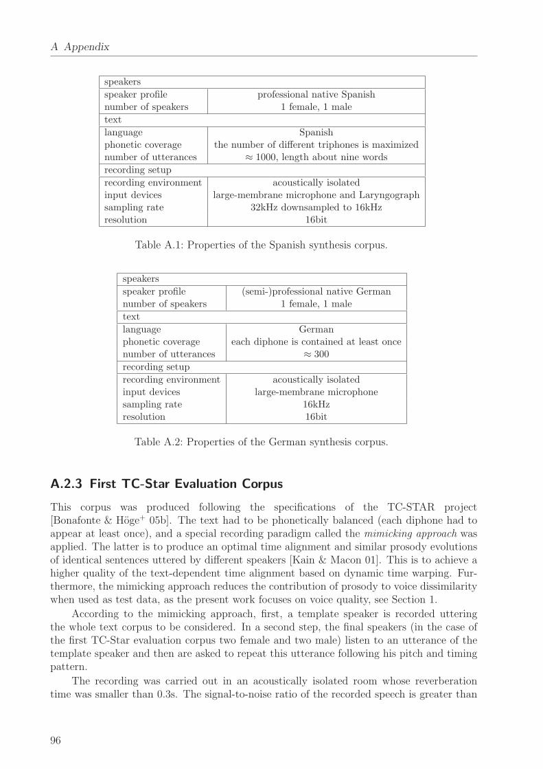
A Appendix
speakers
speaker profile professional native Spanishnumber of speakers 1 female, 1 male
text
language Spanishphonetic coverage the number of different triphones is maximizednumber of utterances ≈ 1000, length about nine words
recording setup
recording environment acoustically isolatedinput devices large-membrane microphone and Laryngographsampling rate 32kHz downsampled to 16kHzresolution 16bit
Table A.1: Properties of the Spanish synthesis corpus.
speakers
speaker profile (semi-)professional native Germannumber of speakers 1 female, 1 male
text
language Germanphonetic coverage each diphone is contained at least oncenumber of utterances ≈ 300
recording setup
recording environment acoustically isolatedinput devices large-membrane microphonesampling rate 16kHzresolution 16bit
Table A.2: Properties of the German synthesis corpus.
A.2.3 First TC-Star Evaluation Corpus
This corpus was produced following the specifications of the TC-STAR project[Bonafonte & Hoge+ 05b]. The text had to be phonetically balanced (each diphone had toappear at least once), and a special recording paradigm called the mimicking approach wasapplied. The latter is to produce an optimal time alignment and similar prosody evolutionsof identical sentences uttered by different speakers [Kain & Macon 01]. This is to achieve ahigher quality of the text-dependent time alignment based on dynamic time warping. Fur-thermore, the mimicking approach reduces the contribution of prosody to voice dissimilaritywhen used as test data, as the present work focuses on voice quality, see Section 1.
According to the mimicking approach, first, a template speaker is recorded utteringthe whole text corpus to be considered. In a second step, the final speakers (in the case ofthe first TC-Star evaluation corpus two female and two male) listen to an utterance of thetemplate speaker and then are asked to repeat this utterance following his pitch and timingpattern.
The recording was carried out in an acoustically isolated room whose reverberationtime was smaller than 0.3s. The signal-to-noise ratio of the recorded speech is greater than
96
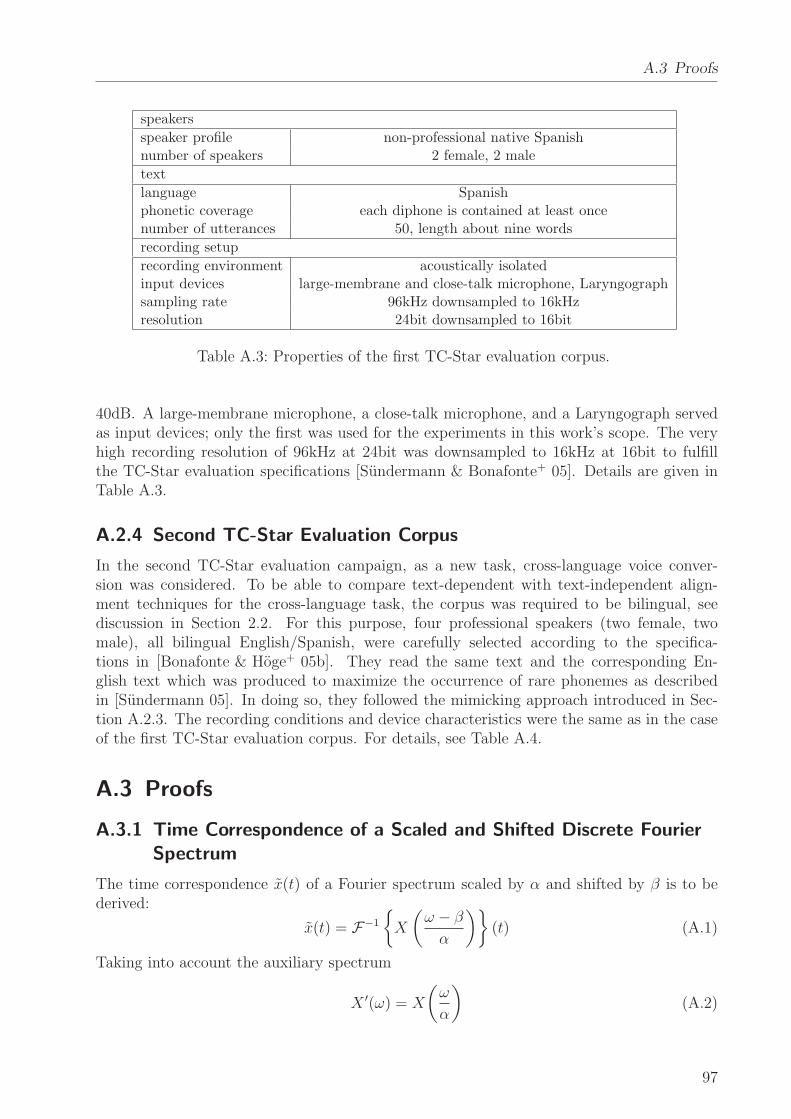
A.3 Proofs
speakers
speaker profile non-professional native Spanishnumber of speakers 2 female, 2 male
text
language Spanishphonetic coverage each diphone is contained at least oncenumber of utterances 50, length about nine words
recording setup
recording environment acoustically isolatedinput devices large-membrane and close-talk microphone, Laryngographsampling rate 96kHz downsampled to 16kHzresolution 24bit downsampled to 16bit
Table A.3: Properties of the first TC-Star evaluation corpus.
40dB. A large-membrane microphone, a close-talk microphone, and a Laryngograph servedas input devices; only the first was used for the experiments in this work’s scope. The veryhigh recording resolution of 96kHz at 24bit was downsampled to 16kHz at 16bit to fulfillthe TC-Star evaluation specifications [Sundermann & Bonafonte+ 05]. Details are given inTable A.3.
A.2.4 Second TC-Star Evaluation Corpus
In the second TC-Star evaluation campaign, as a new task, cross-language voice conver-sion was considered. To be able to compare text-dependent with text-independent align-ment techniques for the cross-language task, the corpus was required to be bilingual, seediscussion in Section 2.2. For this purpose, four professional speakers (two female, twomale), all bilingual English/Spanish, were carefully selected according to the specifica-tions in [Bonafonte & Hoge+ 05b]. They read the same text and the corresponding En-glish text which was produced to maximize the occurrence of rare phonemes as describedin [Sundermann 05]. In doing so, they followed the mimicking approach introduced in Sec-tion A.2.3. The recording conditions and device characteristics were the same as in the caseof the first TC-Star evaluation corpus. For details, see Table A.4.
A.3 Proofs
A.3.1 Time Correspondence of a Scaled and Shifted Discrete Fourier
Spectrum
The time correspondence x(t) of a Fourier spectrum scaled by α and shifted by β is to bederived:
x(t) = F−1
{
X
(
ω − β
α
)}
(t) (A.1)
Taking into account the auxiliary spectrum
X ′(ω) = X
(
ω
α
)
(A.2)
97
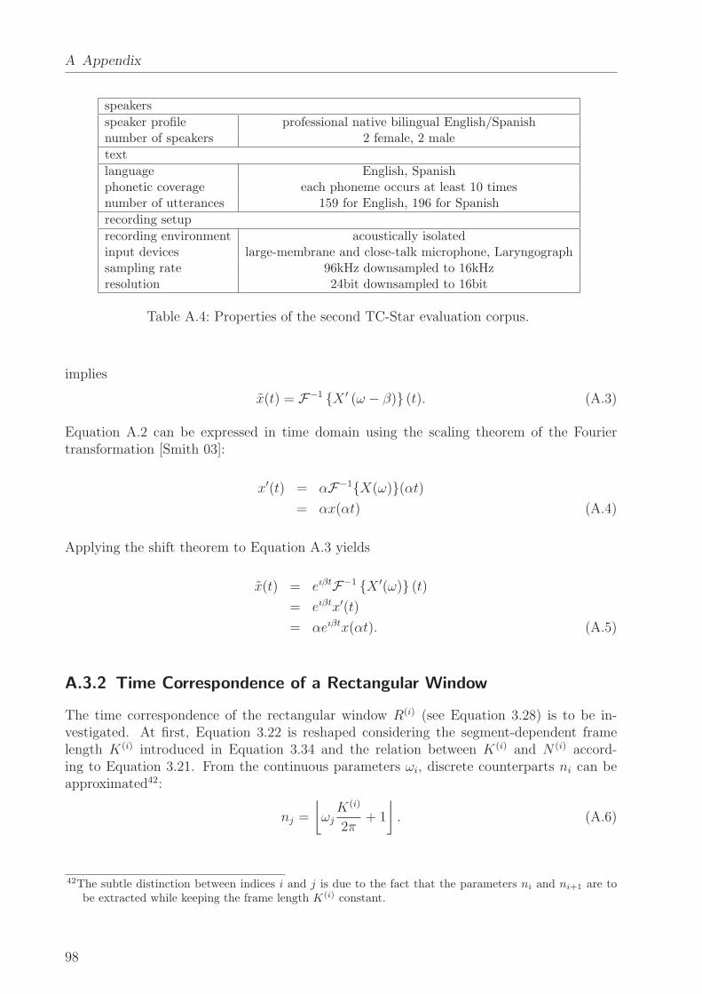
A Appendix
speakers
speaker profile professional native bilingual English/Spanishnumber of speakers 2 female, 2 male
text
language English, Spanishphonetic coverage each phoneme occurs at least 10 timesnumber of utterances 159 for English, 196 for Spanish
recording setup
recording environment acoustically isolatedinput devices large-membrane and close-talk microphone, Laryngographsampling rate 96kHz downsampled to 16kHzresolution 24bit downsampled to 16bit
Table A.4: Properties of the second TC-Star evaluation corpus.
implies
x(t) = F−1 {X ′ (ω − β)} (t). (A.3)
Equation A.2 can be expressed in time domain using the scaling theorem of the Fouriertransformation [Smith 03]:
x′(t) = αF−1{X(ω)}(αt)= αx(αt) (A.4)
Applying the shift theorem to Equation A.3 yields
x(t) = eıβtF−1 {X ′(ω)} (t)
= eıβtx′(t)
= αeıβtx(αt). (A.5)
A.3.2 Time Correspondence of a Rectangular Window
The time correspondence of the rectangular window R(i) (see Equation 3.28) is to be in-vestigated. At first, Equation 3.22 is reshaped considering the segment-dependent framelength K(i) introduced in Equation 3.34 and the relation between K(i) and N (i) accord-ing to Equation 3.21. From the continuous parameters ωi, discrete counterparts ni can beapproximated42:
nj =
⌊
ωjK(i)
2π+ 1
⌋
. (A.6)
42The subtle distinction between indices i and j is due to the fact that the parameters ni and ni+1 are tobe extracted while keeping the frame length K(i) constant.
98
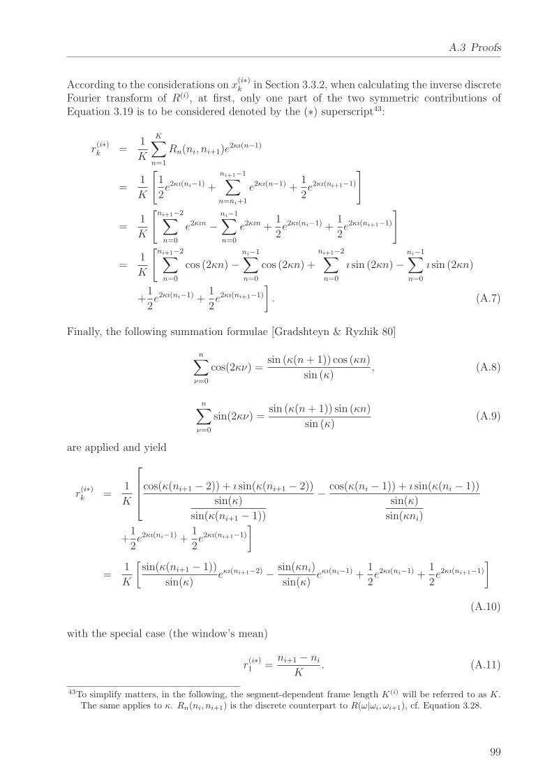
A.3 Proofs
According to the considerations on x(i∗)k in Section 3.3.2, when calculating the inverse discrete
Fourier transform of R(i), at first, only one part of the two symmetric contributions ofEquation 3.19 is to be considered denoted by the (∗) superscript43:
r(i∗)k =
1
K
K∑
n=1
Rn(ni, ni+1)e2κı(n−1)
=1
K
[
1
2e2κı(ni−1) +
ni+1−1∑
n=ni+1
e2κı(n−1) +1
2e2κı(ni+1−1)
]
=1
K
[
ni+1−2∑
n=0
e2κın −ni−1∑
n=0
e2κın +1
2e2κı(ni−1) +
1
2e2κı(ni+1−1)
]
=1
K
[
ni+1−2∑
n=0
cos (2κn) −ni−1∑
n=0
cos (2κn) +
ni+1−2∑
n=0
ı sin (2κn) −ni−1∑
n=0
ı sin (2κn)
+1
2e2κı(ni−1) +
1
2e2κı(ni+1−1)
]
. (A.7)
Finally, the following summation formulae [Gradshteyn & Ryzhik 80]
n∑
ν=0
cos(2κν) =sin (κ(n+ 1)) cos (κn)
sin (κ), (A.8)
n∑
ν=0
sin(2κν) =sin (κ(n+ 1)) sin (κn)
sin (κ)(A.9)
are applied and yield
r(i∗)k =
1
K
cos(κ(ni+1 − 2)) + ı sin(κ(ni+1 − 2))
sin(κ)
sin(κ(ni+1 − 1))
− cos(κ(ni − 1)) + ı sin(κ(ni − 1))
sin(κ)
sin(κni)
+1
2e2κı(ni−1) +
1
2e2κı(ni+1−1)
]
=1
K
[
sin(κ(ni+1 − 1))
sin(κ)eκı(ni+1−2) − sin(κni)
sin(κ)eκı(ni−1) +
1
2e2κı(ni−1) +
1
2e2κı(ni+1−1)
]
(A.10)
with the special case (the window’s mean)
r(i∗)1 =
ni+1 − ni
K. (A.11)
43To simplify matters, in the following, the segment-dependent frame length K(i) will be referred to as K.The same applies to κ. Rn(ni, ni+1) is the discrete counterpart to R(ω|ωi, ωi+1), cf. Equation 3.28.
99
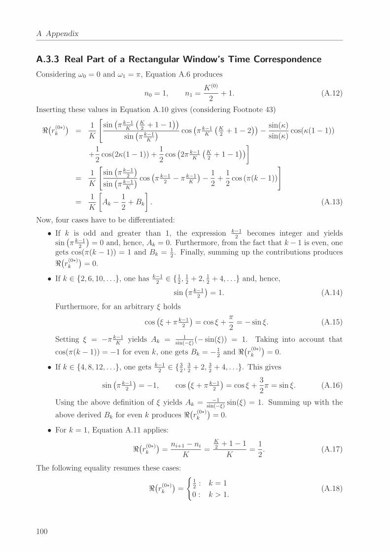
A Appendix
A.3.3 Real Part of a Rectangular Window’s Time Correspondence
Considering ω0 = 0 and ω1 = π, Equation A.6 produces
n0 = 1, n1 =K(0)
2+ 1. (A.12)
Inserting these values in Equation A.10 gives (considering Footnote 43)
ℜ(
r(0∗)k
)
=1
K
[
sin(
π k−1K
(
K2
+ 1 − 1))
sin(
π k−1K
) cos(
π k−1K
(
K2
+ 1 − 2))
− sin(κ)
sin(κ)cos(κ(1 − 1))
+1
2cos(2κ(1 − 1)) +
1
2cos(
2π k−1K
(
K2
+ 1 − 1))
]
=1
K
[
sin(
π k−12
)
sin(
π k−1K
) cos(
π k−12
− π k−1K
)
− 1
2+
1
2cos (π(k − 1))
]
=1
K
[
Ak −1
2+Bk
]
. (A.13)
Now, four cases have to be differentiated:
• If k is odd and greater than 1, the expression k−12
becomes integer and yieldssin(
π k−12
)
= 0 and, hence, Ak = 0. Furthermore, from the fact that k− 1 is even, onegets cos(π(k − 1)) = 1 and Bk = 1
2. Finally, summing up the contributions produces
ℜ(
r(0∗)k
)
= 0.
• If k ∈ {2, 6, 10, . . .}, one has k−12
∈ {12, 1
2+ 2, 1
2+ 4, . . .} and, hence,
sin(
π k−12
)
= 1. (A.14)
Furthermore, for an arbitrary ξ holds
cos(
ξ + π k−12
)
= cos ξ +π
2= − sin ξ. (A.15)
Setting ξ = −π k−1K
yields Ak = 1sin(−ξ)
(− sin(ξ)) = 1. Taking into account that
cos(π(k − 1)) = −1 for even k, one gets Bk = −12
and ℜ(
r(0∗)k
)
= 0.
• If k ∈ {4, 8, 12, . . .}, one gets k−12
∈ {32, 3
2+ 2, 3
2+ 4, . . .}. This gives
sin(
π k−12
)
= −1, cos(
ξ + π k−12
)
= cos ξ +3
2π = sin ξ. (A.16)
Using the above definition of ξ yields Ak = −1sin(−ξ)
sin(ξ) = 1. Summing up with the
above derived Bk for even k produces ℜ(
r(0∗)k
)
= 0.
• For k = 1, Equation A.11 applies:
ℜ(
r(0∗)k
)
=ni+1 − ni
K=
K2
+ 1 − 1
K=
1
2. (A.17)
The following equality resumes these cases:
ℜ(
r(0∗)k
)
=
{
12
: k = 1
0 : k > 1.(A.18)
100
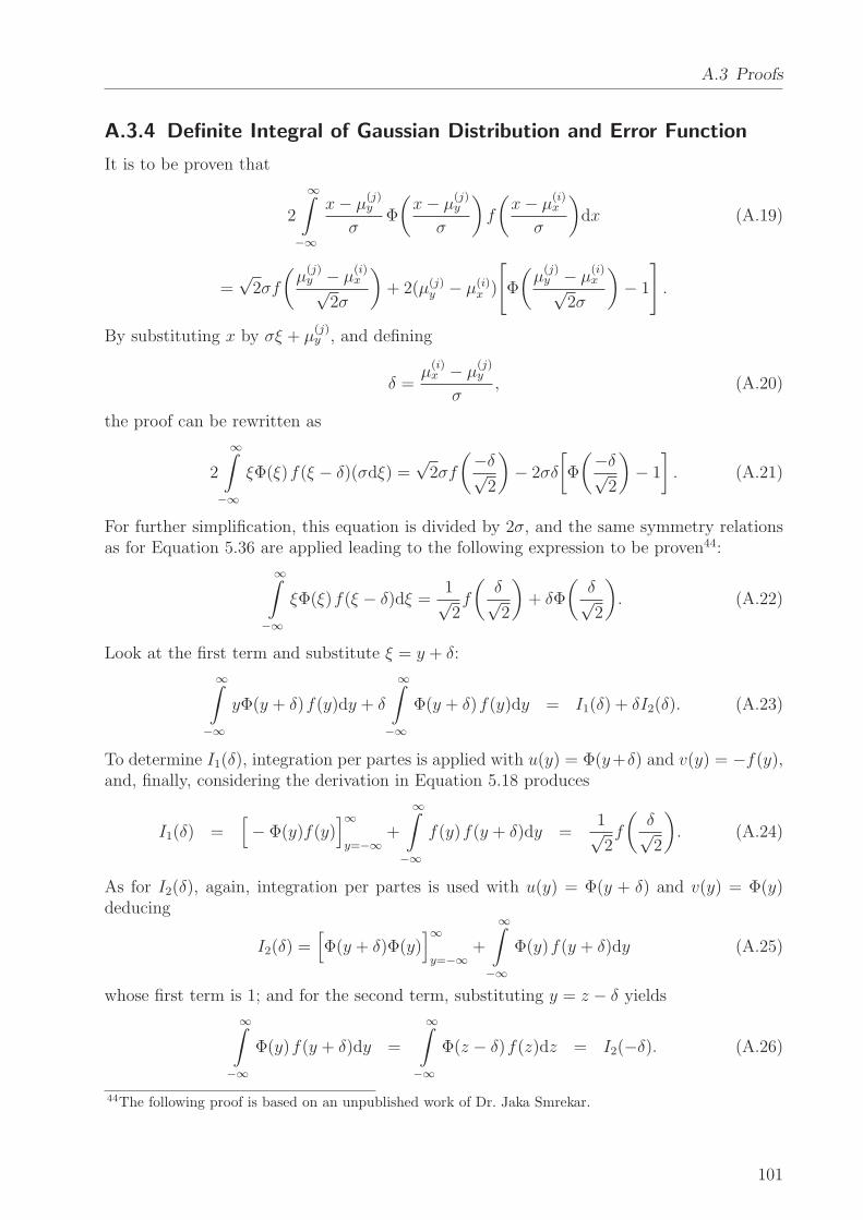
A.3 Proofs
A.3.4 Definite Integral of Gaussian Distribution and Error Function
It is to be proven that
2
∞∫
−∞
x− µ(j)y
σΦ
(
x− µ(j)y
σ
)
f
(
x− µ(i)x
σ
)
dx (A.19)
=√
2σf
(
µ(j)y − µ
(i)x√
2σ
)
+ 2(µ(j)y − µ(i)
x )
[
Φ
(
µ(j)y − µ
(i)x√
2σ
)
− 1
]
.
By substituting x by σξ + µ(j)y , and defining
δ =µ
(i)x − µ
(j)y
σ, (A.20)
the proof can be rewritten as
2
∞∫
−∞
ξΦ(ξ)f(ξ − δ)(σdξ) =√
2σf
(−δ√2
)
− 2σδ
[
Φ
(−δ√2
)
− 1
]
. (A.21)
For further simplification, this equation is divided by 2σ, and the same symmetry relationsas for Equation 5.36 are applied leading to the following expression to be proven44:
∞∫
−∞
ξΦ(ξ)f(ξ − δ)dξ =1√2f
(
δ√2
)
+ δΦ
(
δ√2
)
. (A.22)
Look at the first term and substitute ξ = y + δ:
∞∫
−∞
yΦ(y + δ)f(y)dy + δ
∞∫
−∞
Φ(y + δ)f(y)dy = I1(δ) + δI2(δ). (A.23)
To determine I1(δ), integration per partes is applied with u(y) = Φ(y+δ) and v(y) = −f(y),and, finally, considering the derivation in Equation 5.18 produces
I1(δ) =[
− Φ(y)f(y)]∞
y=−∞+
∞∫
−∞
f(y)f(y + δ)dy =1√2f
(
δ√2
)
. (A.24)
As for I2(δ), again, integration per partes is used with u(y) = Φ(y + δ) and v(y) = Φ(y)deducing
I2(δ) =[
Φ(y + δ)Φ(y)]∞
y=−∞+
∞∫
−∞
Φ(y)f(y + δ)dy (A.25)
whose first term is 1; and for the second term, substituting y = z − δ yields
∞∫
−∞
Φ(y)f(y + δ)dy =
∞∫
−∞
Φ(z − δ)f(z)dz = I2(−δ). (A.26)
44The following proof is based on an unpublished work of Dr. Jaka Smrekar.
101
A Appendix
Inserting this into Equation A.25 gives
I2(δ) + I2(−δ) = 1. (A.27)
Now, the term I2(δ) − I2(−δ) is to be computed which is by definition
I2(δ) − I2(−δ) =
∞∫
−∞
f(x)[
Φ(x+ δ) − Φ(x− δ)]
dx
=
∞∫
−∞
f(x)
x+δ∫
−x−δ
f(u)du dx. (A.28)
Substituting u = y + x, changing the integration order, applying Equation 5.18, and substi-tuting z = y√
2produces
I2(δ) − I2(−δ) =
∞∫
−∞
f(x)
δ∫
−δ
f(y + x)dy dx
=
δ∫
−δ
∞∫
−∞
f(x)f(y + x)dx dy
=
δ∫
−δ
1√2f
(
y√2
)
dy
=
δ√2
∫
− δ√2
f(z)dz = 2
δ√2
∫
0
f(z)dz. (A.29)
Adding Equations A.27 and A.29 yields
I2(δ) =1
2+
δ√2
∫
0
f(z)dz
=
0∫
−∞
f(z)dz +
δ√2
∫
0
f(z)dz
= Φ
(
δ√2
)
. (A.30)
The latter and Equation A.24 add up to the expression in Equation A.23 finishing the proof.
102
A.3 Proofs
A.3.5 Limit of Expected Minimal Distances of Random Vectors
Distributed According to the Gaussian Mixture Model
It is to be proven that
limN→∞
EN(D) = limN→∞
1
σ
I∑
i=1
α(i)x
∞∫
−∞
EN(D|x)f(
x− µ(i)x
σ
)
dx = 0 (A.31)
with
EN(D|x) =N
σ
J∑
j=1
α(j)y
x∫
−∞
(x−y)f(
y−µ(j)y
σ
)(
1+Φ
(
y−µ(j)y
σ
)
−Φ
(
2x−y−µ(j)y
σ
))N−1
dy
−∞∫
x
(x− y)f
(
y − µ(j)y
σ
)(
1 − Φ
(
y − µ(j)y
σ
)
+ Φ
(
2x− y − µ(j)y
σ
))N−1
dy
. (A.32)
Changing the orders of limit, summation, and integration, Equation A.31 becomes
limN→∞
EN(D) =I∑
i=1
J∑
j=1
α(i)x α
(j)y lim
N→∞E
(i,j)N (D) (A.33)
with
E(i,j)N (D) =
N
σ2
∞∫
−∞
x∫
−∞
f
(
x−µ(i)x
σ
)
(x−y)f(
y−µ(j)y
σ
)(
1+Φ
(
y−µ(j)y
σ
)
−Φ
(
2x−y−µ(j)y
σ
))N−1
dy dx
−N
σ2
∞∫
−∞
∞∫
x
f
(
x− µ(i)x
σ
)
(x−y)f(
y − µ(j)y
σ
)(
1−Φ
(
y − µ(j)y
σ
)
+Φ
(
2x− y − µ(j)y
σ
))N−1
dy dx.
(A.34)
Substituting u =y−µ
(j)y
σand v = 2
x−µ(j)y
σ− u and using Equation A.20, this can be rewritten
as45
E(i,j)N (D) =
Nσ
4
∞∫
−∞
v∫
−∞
f
(
u+ v
2− δ
)
(v − u)f(u)(1 + Φ(u) − Φ(v))N−1du dv (A.35)
− Nσ
4
∞∫
−∞
∞∫
v
f
(
u+ v
2− δ
)
(v − u)f(u)(1 − Φ(u) + Φ(v))N−1du dv.
Applying integration per partes in the inner integrals [the terms Nf(u)(1+Φ(u)−Φ(v))N−1
and −Nf(u)(1−Φ(u)+Φ(v))N−1 are differentials of (1+Φ(u)−Φ(v))N and (1−Φ(u)+Φ(v))N
with respect to u] yields the equality
E(i,j)N (D) =
σ
4
∞∫
−∞
v∫
−∞
(1 + Φ(u) − Φ(v))Nf
(
u+ v
2− δ
)((
u+ v
2− δ
)
u− v
2+ 1
)
du dv
45The following proof is based on an unpublished work of Dr. Jaka Smrekar.
103
A Appendix
+σ
4
∞∫
−∞
∞∫
v
(1 − Φ(u) + Φ(v))Nf
(
u+ v
2− δ
)((
u+ v
2− δ
)
v − u
2+ 1
)
du dv (A.36)
Switching the roles of u and v in the second summand applying Fubini’s theorem [Rudin 87],one obtains
E(i,j)N (D) =
σ
2
∞∫
−∞
v∫
−∞
(1 + Φ(u) − Φ(v))Nf
(
u+ v
2− δ
)
du dv. (A.37)
Note that for u ≤ v, the expression 1 + Φ(u) − Φ(v) is at most 1, and therefore
limN→∞
(1 + Φ(u) − Φ(v))N =
{
1 : u = v
0 : otherwise.(A.38)
A double application of Lebesgue’s dominated convergence theorem [Browder 96] yields
limN→∞
E(i,j)N (D) = 0 (A.39)
which, inserted into Equation A.33, finishes the proof.
104
References
[Abe & Nakamura+ 88] M. Abe, S. Nakamura, K. Shikano, H. Kuwabara: Voice Conversionthrough Vector Quantization. In Proc. of the ICASSP, New York, USA, 1988.
[Abe & Shikano+ 90] M. Abe, K. Shikano, H. Kuwabara: Cross-Language Voice Conversion. InProc. of the ICASSP, Albuquerque, USA, 1990.
[Acero & Stern 91] A. Acero, R. Stern: Robust Speech Recognition by Normalization of the Acous-tic Space. In Proc. of the ICASSP, Toronto, Canada, 1991.
[Aguero & Adell+ 06] P. Aguero, J. Adell, A. Bonafonte: Prosody Generation for Speech-to-SpeechTranslation. In Proc. of the ICASSP, Toulouse, France, 2006.
[Ainsworth & Paliwal+ 84] W. Ainsworth, K. Paliwal, H. Foster: Problems with Dynamic Fre-quency Warping as a Technique for Speaker-Independent Vowel Classification. Proc. of theInstitute of Acoustics, Vol. 6, No. 4, 1984.
[Ali & Spiegel+ 99] A. Ali, J. Spiegel, P. Mueller, G. Haentjens, J. Berman: An Acoustic-PhoneticFeature-Based System for Automatic Phoneme Recognition in Continuous Speech. In Proc. ofthe ISCAS, Orlando, USA, 1999.
[Arfken 85] G. Arfken: Mathematical Methods for Physicists. Academic Press, Orlando, USA,1985.
[Atal & Hanauer 71] B. Atal, S. Hanauer: Speech Analysis and Synthesis by Linear Prediction.Journal of the Acoustical Society of America, Vol. 50, No. 2, 1971.
[Avriel 76] M. Avriel: Nonlinear Programming: Analysis and Methods. Prentice Hall, EnglewoodCliffs, USA, 1976.
[Banno & Hata+ 07] H. Banno, H. Hata, M. Morise, T. Takahashi, T. Irino, H. Kawahara: Im-plementation of Realtime STRAIGHT Speech Manipulation System: Report on Its First Imple-mentation. Acoustical Science and Technology, Vol. 28, No. 3, 2007.
[Barbosa 97] A. Barbosa. A New Mexican Spanish Voice for the Festival Text to Speech System.Master’s thesis, University of the Americas, Puebla, Mexico, 1997.
[Bennett 05] C. Bennett: Large Scale Evaluation of Corpus-Based Synthesizers: Results andLessons from the Blizzard Challenge 2005. In Proc. of the Interspeech, Lisbon, Portugal, 2005.
[Bernadin & Foo 06] S. Bernadin, S. Foo: Wavelet Processing for Pitch Period Estimation. InProc. of the Southeastern Symposium on System Theory, Cookeville, USA, 2006.
[Beutnagel & Conkie+ 99] M. Beutnagel, A. Conkie, J. Schroeter, Y. Stylianou, A. Syrdal: TheAT&T Next-Gen TTS System. In Proc. of the Joint Meeting of ASA, EAA, and DAGA, Berlin,Germany, 1999.
[Black & Lenzo 01] A. Black, K. Lenzo: Optimal Data Selection for Unit Selection Synthesis. InProc. of the ISCA Workshop on Speech Synthesis, Perthshire, UK, 2001.
[Black & Lenzo 03] A. Black, K. Lenzo: Building Synthetic Voices. Carnegie Mellon University,Pittsburgh, USA, 2003.
References
[Boersma 01] P. Boersma: Praat, a System for Doing Phonetics by Computer. Glot International,Vol. 5, No. 9/10, 2001.
[Bonafonte & Banchs+ 06] A. Bonafonte, R. Banchs, A. Moreno: TC-STAR Workshop on Speech-to-Speech Translation. Barcelona, Spain, 2006.
[Bonafonte & Esquerra+ 98] A. Bonafonte, I. Esquerra, A. Febrer, J. Fonollosa, F. Vallverdu: TheUPC Text-to-Speech System for Spanish and Catalan. In Proc. of the ICSLP, Sydney, Australia,1998.
[Bonafonte & Hoge+ 05a] A. Bonafonte, H. Hoge, I. Kiss, A. Moreno, D. Sundermann, U. Ziegen-hain, J. Adell, P. Aguero, H. Duxans, D. Erro, J. Nurminen, J. Perez, G. Strecha, M. Umbert,X. Wang. TC-STAR: TTS Progress Report. Technical report, 2005.
[Bonafonte & Hoge+ 05b] A. Bonafonte, H. Hoge, H. Tropf, A. Moreno, H. v. d. Heuvel,D. Sundermann, U. Ziegenhain, J. Perez, I. Kiss. TC-Star: Specifications of Language Resourcesfor Speech Synthesis. Technical report, 2005.
[Boril & Fousek+ 06] H. Boril, P. Fousek, D. Sundermann, P. Cerva, J. Zd’ansky: Lombard SpeechRecognition: A Comparative Study. In Proc. of the Czech-German Workshop, Prague, CzechRepublic, 2006.
[Boudelaa & Meftah 96] S. Boudelaa, M. Meftah: Cross-Language Effects of Lexical Stress inWord Recognition: The Case of Arabic English Bilinguals. In Proc. of the ICSLP, Philadelphia,USA, 1996.
[Braun & Masthoff 02] A. Braun, H. Masthoff: Phonetics and Its Applications. Steiner, Stuttgart,Germany, 2002.
[Browder 96] A. Browder: Mathematical Analysis: An Introduction. Springer, New York, USA,1996.
[Ceyssens & Verhelst+ 02] T. Ceyssens, W. Verhelst, P. Wambacq: A Strategy for Pitch Conver-sion and Its Evaluation. In Proc. of the SPS, Leuven, Belgium, 2002.
[Charpentier & Moulines 88] F. Charpentier, E. Moulines: Text-to-Speech Algorithms Based onFFT Synthesis. In Proc. of the ICASSP, New York, USA, 1988.
[Charpentier & Stella 86] F. Charpentier, M. Stella: Diphone Synthesis Using an Overlap-AddTechnique for Speech Waveforms Concatenation. In Proc. of the ICASSP, Tokyo, Japan, 1986.
[Cheng & O’Shaughnessy 89] Y. Cheng, D. O’Shaughnessy: Automatic and Reliable Estimationof Glottal Closure Instant and Period. IEEE Trans. on Acoustics, Speech and Signal Processing,Vol. 37, No. 12, 1989.
[Childers & Lee 91] D. Childers, C. Lee: Vocal Quality Factors: Analysis, Synthesis, and Percep-tion. Journal of the Acoustical Society of America, Vol. 90, No. 5, 1991.
[Childers & Wong 94] D. Childers, C.F. Wong: Measuring and Modeling Vocal Source-Tract In-teraction. IEEE Trans. on Biomedical Engineering, Vol. 41, No. 7, 1994.
[Cho & Kim+ 98] Y. Cho, M. Kim, S. Kim: A Spectrally Mixed Excitation (SMX) Vocoder withRobust Parameter Determination. In Proc. of the ICASSP, Seattle, USA, 1998.
[Cohen & Kamm+ 95] J. Cohen, T. Kamm, A. Andreou: Vocal Tract Normalization in SpeechRecognition: Compensating for Systematic Speaker Variability. Journal of the Acoustical Societyof America, Vol. 97, No. 5, 1995.
[Cole 98] R. Cole: Survey of the State of the Art in Human Language Technology. Giardini Editorie Stampatori, Pisa, Italy, 1998.
106
References
[Cormen & Leiserson+ 90] T. Cormen, C. Leiserson, R. Rivest: Introduction to Algorithms. MITPress, Cambridge, USA, 1990.
[David & Nagaraja 03] H. David, H. Nagaraja: Order Statistics. Wiley, New York, USA, 2003.
[de Boor 78] C. de Boor: A Practical Guide to Splines. Springer, New York, USA, 1978.
[de los Galanes & Savoji+ 94] F. de los Galanes, M. Savoji, J. Pardo: New Algorithm for Spec-tral Smoothing and Envelope Modification for LP-PSOLA Synthesis. In Proc. of the ICASSP,Adelaide, Australia, 1994.
[Deller & Proakis+ 93] J. Deller, J. Proakis, J. Hansen: Discrete-Time Processing of Speech Sig-nals. Prentice Hall, Englewood Cliffs, USA, 1993.
[Dharanipragada & Gopinath+ 98] S. Dharanipragada, R. Gopinath, B. Rao: Techniques for Cap-turing Temporal Variations in Speech Signals with Fixed-Rate Processing. In Proc. of the ICSLP,Sydney, Australia, 1998.
[Dolson 94] M. Dolson: The Pitch of Speech as a Function of Linguistic Community. MusicPerception, Vol. 11, No. 1, 1994.
[Donovan & Woodland 95] R. Donovan, P. Woodland: Improvements in an HMM-Based SpeechSynthesiser. In Proc. of the Eurospeech, Madrid, Spain, 1995.
[Duda & Hart 73] R. Duda, P. Hart: Pattern Classification and Scene Analysis. Wiley, New York,USA, 1973.
[Durbin 60] J. Durbin: The Fitting of Time-Series Models. Revue de l’Institut International deStatistique, Vol. 28, No. 3, 1960.
[Dutoit & Pagel+ 96] T. Dutoit, V. Pagel, N. Pierret, F. Bataille, O. v. d. Vrecken: The MBROLAProject: Towards a Set of High Quality Speech Synthesizers Free of Use for Non CommercialPurposes. In Proc. of the ICSLP, Philadelphia, USA, 1996.
[Dutoit 93] T. Dutoit. High Quality Text-To-Speech Synthesis of the French Language. Ph.D.thesis, Polytechnic Faculty of Mons, Mons, Belgium, 1993.
[Duxans & Bonafonte 03] H. Duxans, A. Bonafonte: Estimation of GMM in Voice ConversionIncluding Unaligned Data. In Proc. of the Eurospeech, Geneva, Switzerland, 2003.
[Eide & Gish 96] E. Eide, H. Gish: A Parametric Approach to Vocal Tract Length Normalization.In Proc. of the ICASSP, Atlanta, USA, 1996.
[Eide & Picheny 06] E. Eide, M. Picheny: Towards Pooled-Speaker Concatenative Text-to-Speech.In Proc. of the ICASSP, Toulouse, France, 2006.
[ETSI 99] ETSI. Adaptive Multi-Rate (AMR) Speech Transcoding. Technical report, EuropeanTelecommunications Standards Institute, Sophia Antipolis, France, 1999.
[Evermann & Chan+ 05] G. Evermann, H. Chan, M. Gales, B. Jia, D. Mrva, P. Woodland, K. Yu:Training LVCSR Systems on Thousands of Hours of Data. In Proc. of the ICASSP, Philadelphia,USA, 2005.
[Fallside & Woods 85] F. Fallside, W. Woods: Computer Speech Processing. Prentice Hall, Engle-wood Cliffs, USA, 1985.
[Faltlhauser & Pfau+ 00] R. Faltlhauser, T. Pfau, G. Ruske: On-Line Speaking Rate EstimationUsing Gaussian Mixture Models. In Proc. of the ICASSP, Istanbul, Turkey, 2000.
[Fant 70] G. Fant: Acoustic Theory of Speech Production. Mouton, The Hague, Netherlands, 1970.
107
References
[Fischer & Kunzmann 06] V. Fischer, S. Kunzmann: From Pre-Recorded Prompts to CorporateVoices: On the Migration of Interactive Voice Response Applications. In Proc. of the Interspeech,Pittsburgh, USA, 2006.
[Fisher & Doddington+ 86] W. Fisher, G. Doddington, K. Goudie-Marshall: The DARPA SpeechRecognition Research Database: Specifications and Status. In Proc. of the DARPA Workshopon Speech Recognition, Palo Alto, USA, 1986.
[Furui & Nakamura+ 06] S. Furui, M. Nakamura, K. Iwano: Why is automatic recognition ofspontaneous speech so difficult? In Proc. of the Symposium on Large-Scale Knowledge Resources,Tokyo, Japan, 2006.
[Gauss 09] C. Gauss: Theoria Motus Corporum Coelestium in Sectionibus Conicis Solem Ambien-tium. Perthes and Besser, Hamburg, Germany, 1809.
[Germann 06] U. Germann. An Iterative Approach to Pitch-Marking of Speech Signals withoutElectroglottographic Data. Technical report, University of Toronto, Toronto, Canada, 2006.
[Gollan & Bisani+ 05] C. Gollan, M. Bisani, S. Kanthak, R. Schluter, H. Ney: Cross DomainAutomatic Transcription on the TC-Star EPPS Corpus. In Proc. of the ICASSP, Philadelphia,USA, 2005.
[Goncharoff & Gries 98] V. Goncharoff, P. Gries: An Algorithm for Accurately Marking PitchPulses in Speech Signals. In Proc. of the SIP, Las Vegas, USA, 1998.
[Gradshteyn & Ryzhik 80] I. Gradshteyn, I. Ryzhik: Table of Integrals, Series and Products. Aca-demic Press, New York, USA, 1980.
[Gray & Markel 76] A. Gray, J. Markel: Distance Measures for Speech Processing. IEEE Trans.on Acoustics, Speech and Signal Processing, Vol. 24, No. 5, 1976.
[Gray 18] H. Gray: Anatomy of the Human Body. Lea and Febiger, Philadelphia, USA, 1918.
[Griffin 87] D. Griffin. Multi-Band Excitation Vocoder. Ph.D. thesis, Massachusetts Institute ofTechnology, Cambridge, USA, 1987.
[Hagen 94] R. Hagen: Spectral Quantization of Cepstral Coefficients. In Proc. of the ICASSP,Adelaide, Australia, 1994.
[Hain 01] T. Hain. Hidden Model Sequence Models for Automatic Speech Recognition. Ph.D. thesis,Cambridge University, Cambridge, UK, 2001.
[Hamon & Moulines+ 89] C. Hamon, E. Moulines, F. Charpentier: A Diphone Synthesis SystemBased on Time-Domain Prosodic Modification of Speech. In Proc. of the ICASSP, Glasgow, UK,1989.
[Hermansky & Morgan 94] H. Hermansky, N. Morgan: RASTA processing of speech. IEEE Trans.on Speech and Audio Processing, Vol. 2, No. 4, 1994.
[Hermansky 90] H. Hermansky: Perceptual Linear Predictive (PLP) Analysis of Speech. Journalof the Acoustical Society of America, Vol. 87, No. 4, 1990.
[Hillebrand 02] F. Hillebrand: GSM and UMTS: The Creation of Global Mobile Communications.Wiley, New York, USA, 2002.
[Hoffmann & Jokisch+ 03] R. Hoffmann, O. Jokisch, D. Hirschfeld, G. Strecha, H. Kruschke,U. Kordon: A Multilingual TTS System with Less than 1 Megabyte Footprint for EmbeddedApplications. In Proc. of the ICASSP, Hong Kong, China, 2003.
[Hoge & Kotnik+ 06] H. Hoge, B. Kotnik, Z. Kacic, H. Pfitzinger: Evaluation of Pitch MarkingAlgorithms. In Proc. of the ITG, Kiel, Germany, 2006.
108
References
[Hoge 02] H. Hoge: Project Proposal TC-STAR - Make Speech to Speech Translation Real. InProc. of the LREC, Las Palmas, Spain, 2002.
[Hogg & McKean+ 95] R. Hogg, J. McKean, A. Craig: Introduction to Mathematical Statistics.Prentice Hall, Englewood Cliffs, USA, 1995.
[Horne 00] M. Horne: Prosody: Theory and Experiment. Kluwer Academic Publishers, Dordrecht,Netherlands, 2000.
[Hosom & Kain+ 03] J. Hosom, A. Kain, T. Mishra, J. v. Santen, M. Fried-Oken, J. Staehely:Intelligibility of Modifications to Dysarthric Speech. In Proc. of the ICASSP, Hong Kong, China,2003.
[Hunt & Black 96] A. Hunt, A. Black: Unit Selection in a Concatenative Speech Synthesis SystemUsing a Large Speech Database. In Proc. of the ICASSP, Atlanta, USA, 1996.
[Inanoglu 03] Z. Inanoglu. Transforming Pitch in a Voice Conversion Framework. Master’s thesis,University of Cambridge, Cambridge, UK, 2003.
[Itakura 75] F. Itakura: Line Spectrum Representation of Linear Predictive Coefficients of SpeechSignals. Journal of the Acoustical Society of America, Vol. 57, 1975.
[ITU 96] ITU. Methods for Subjective Determination of Transmission Quality. Technical ReportITU-T Recommendation P.800, International Telecommunication Union, Geneva, Switzerland,1996.
[Kain & Macon 98] A. Kain, M. Macon: Spectral Voice Conversion for Text-to-Speech Synthesis.In Proc. of the ICASSP, Seattle, USA, 1998.
[Kain & Macon 01] A. Kain, M. Macon: Design and Evaluation of a Voice Conversion AlgorithmBased on Spectral Envelope Mapping and Residual Prediction. In Proc. of the ICASSP, SaltLake City, USA, 2001.
[Kain 01] A. Kain. High Resolution Voice Transformation. Ph.D. thesis, Oregon Health and ScienceUniversity, Portland, USA, 2001.
[Kawahara & Estill+ 01] H. Kawahara, J. Estill, O. Fujimura: Aperiodicity Extraction and Con-trol Using Mixed Mode Excitation and Group Delay Manipulation for a High Quality SpeechAnalysis, Modification and Synthesis System STRAIGHT. In Proc. of the MAVEBA, Firenze,Italy, 2001.
[Kotnik & Hoge+ 06] B. Kotnik, H. Hoge, Z. Kacic: Evaluation of Pitch Detection Algorithms inAdverse Conditions. In Proc. of the Speech Prosody, Dresden, Germany, 2006.
[Kotnik 06] B. Kotnik: First PMA/PDA Evaluation Campaign. In Proc. of the AST, Maribor,Slovenia, 2006.
[Kuwabara & Sagisaka 95] H. Kuwabara, Y. Sagisaka: Acoustic Characteristics of Speaker Indi-viduality: Control and Conversion. Speech Communication, Vol. 16, No. 2, 1995.
[Ladefoged 90] P. Ladefoged: The Revised International Phonetic Alphabet. Language, Vol. 66,No. 3, 1990.
[Lee & Rose 96] L. Lee, R. Rose: Speaker Normalization Using Efficient Frequency Warping Pro-cedures. In Proc. of the ICASSP, Atlanta, USA, 1996.
[Lee & Wu 06] C. Lee, C. Wu: Map-Based Adaptation for Speech Conversion Using AdaptationData Selection and Non-Parallel Training. In Proc. of the Interspeech, Pittsburgh, USA, 2006.
[Lewis & Tatham 99] E. Lewis, M. Tatham: Word and Syllable Concatenation in Text-to-SpeechSynthesis. In Proc. of the Eurospeech, Budapest, Hungary, 1999.
109
References
[Macon 96] M. Macon. Speech Synthesis Based on Sinusoidal Modeling. Ph.D. thesis, GeorgiaInstitute of Technology, Atlanta, USA, 1996.
[Makhoul 75] J. Makhoul: Linear Prediction: A Tutorial Review. Proceedings of the IEEE, Vol. 63,No. 4, 1975.
[Markel & Gray 76] J. Markel, A. Gray: Linear Prediction of Speech. Springer, New York, USA,1976.
[Mashimo & Toda+ 01] M. Mashimo, T. Toda, K. Shikano, N. Campbell: Evaluation of Cross-Language Voice Conversion Based on GMM and STRAIGHT. In Proc. of the Eurospeech, Aal-borg, Denmark, 2001.
[Masuko 02] T. Masuko. HMM-Based Speech Synthesis and Its Applications. Ph.D. thesis, TokyoInstitute of Technology, Tokyo, Japan, 2002.
[Matsumoto & Wakita 86] H. Matsumoto, H. Wakita: Vowel Normalization by Frequency WarpedSpectral Matching. Speech Communication, Vol. 5, No. 2, 1986.
[Mattheyses & Verhelst+ 06] W. Mattheyses, W. Verhelst, P. Verhoeve: Robust Pitch Markingfor Prosodic Modification of Speech Using TD-PSOLA. In Proc. of the SPS-DARTS, Antwerp,Belgium, 2006.
[McAulay & Quatieri 86] R. McAulay, T. Quatieri: Speech Analysis-Synthesis Based on a Sinu-soidal Representation. IEEE Trans. on Acoustics, Speech and Signal Processing, Vol. 34, 1986.
[McDonough & Byrne+ 98] J. McDonough, W. Byrne, X. Luo: Speaker Normalization with All-Pass Transforms. In Proc. of the ICSLP, Sydney, Australia, 1998.
[Meilgaard & Civille+ 99] M. Meilgaard, G. Civille, B. Carr: Sensory Evaluation Techniques. CRCPress, Boca Raton, USA, 1999.
[Molau & Kanthak+ 00] S. Molau, S. Kanthak, H. Ney: Efficient Vocal Tract Normalization inAutomatic Speech Recognition. In Proc. of the ESSV, Cottbus, Germany, 2000.
[Molau 02] S. Molau. Normalization in the Acoustic Feature Space for Improved Speech Recognition.Ph.D. thesis, RWTH Aachen, Aachen, Germany, 2002.
[Montgomery 96] D. Montgomery: Introduction to Statistical Quality Control. Wiley, New York,USA, 1996.
[Mostefa & Garcia+ 06] D. Mostefa, M. Garcia, O. Hamon, N. Moreau. TC-Star: EvaluationReport. Technical report, 2006.
[Moulines & Charpentier 88] E. Moulines, F. Charpentier: Diphone Synthesis Using a MultipulseLPC Technique. In Proc. of the FASE Symposium, Edinburgh, UK, 1988.
[Moulines & Sagisaka 95] E. Moulines, Y. Sagisaka: Voice Conversion: State of the Art and Per-spectives. Speech Communication, Vol. 16, No. 2, 1995.
[Nakagiri & Toda+ 06] M. Nakagiri, T. Toda, H. Kashioka, K. Shikano: Improving Body Transmit-ted Unvoiced Speech with Statistical Voice Conversion. In Proc. of the Interspeech, Pittsburgh,USA, 2006.
[Nakamura & Toda+ 06] K. Nakamura, T. Toda, H. Saruwatari, K. Shikano: Speaking Aid Systemfor Total Laryngectomees Using Voice Conversion of Body Transmitted Artificial Speech. In Proc.of the Interspeech, Pittsburgh, USA, 2006.
[Ney & Welling+ 98] H. Ney, L. Welling, S. Ortmanns, K. Beulen, F. Wessel: The RWTH LargeVocabulary Continuous Speech Recognition System. In Proc. of the ICASSP, Seattle, USA,1998.
110
References
[Nicolao & Drioli+ 06] M. Nicolao, C. Drioli, P. Cosi: Voice GMM Modelling for FESTI-VAL/MBROLA Emotive TTS Synthesis. In Proc. of the Interspeech, Pittsburgh, USA, 2006.
[Nolan 83] F. Nolan: The Phonetic Bases of Speech Recognition. Cambridge University Press,Cambridge, UK, 1983.
[Nurminen & Tian+ 06] J. Nurminen, J. Tian, V. Popa: Novel Method for Data Clustering andMode Selection with Application in Voice Conversion. In Proc. of the Interspeech, Pittsburgh,USA, 2006.
[Ohtani & Toda+ 06] Y. Ohtani, T. Toda, H. Saruwatari, K. Shikano: Maximum Likelihood VoiceConversion Based on GMM with STRAIGHT Mixed Excitation. In Proc. of the Interspeech,Pittsburgh, USA, 2006.
[Oppenheim & Schafer 89] A. Oppenheim, R. Schafer: Discrete-Time Signal Processing. PrenticeHall, Englewood Cliffs, USA, 1989.
[Paliwal 95] K. Paliwal: Interpolation Properties of Linear Prediction Parametric Representations.In Proc. of the Eurospeech, Madrid, Spain, 1995.
[Papamichalis 87] P. Papamichalis: Practical Approaches to Speech Coding. Prentice Hall, Engle-wood Cliffs, USA, 1987.
[Picone 93] J. Picone: Signal Modeling Techniques in Speech Recognition. Proc. of the IEEE,Vol. 81, No. 9, 1993.
[Pitz & Ney 05] M. Pitz, H. Ney: Vocal Tract Normalization Equals Linear Transformation inCepstral Space. IEEE Trans. on Speech and Audio Processing, Vol. 13, No. 5, 2005.
[Preparata & Shamos 85] F. Preparata, M. Shamos: Computational Geometry - an Introduction.Springer, New York, USA, 1985.
[Pye & Woodland 97] D. Pye, P. Woodland: Experiments in Speaker Normalization and Adap-tation for Large Vocabulary Speech Recognition. In Proc. of the ICASSP, Munich, Germany,1997.
[Qin & Chen+ 05] L. Qin, G. Chen, Z. Ling, L. Dai: An Improved Spectral and Prosodic Transfor-mation Method in STRAIGHT-Based Voice Conversion. In Proc. of the ICASSP, Philadelphia,USA, 2005.
[Rabiner & Juang 93] L. Rabiner, B. Juang: Fundamentals of Speech Recognition. Prentice Hall,Englewood Cliffs, USA, 1993.
[Rabiner & Rosenberg+ 78] L. Rabiner, A. Rosenberg, S. Levinson: Considerations in DynamicTime Warping Algorithms for Discrete Word Recognition. IEEE Trans. on Acoustics, Speechand Signal Processing, Vol. 26, No. 6, 1978.
[Reynolds 94] D. Reynolds: An Application of Recurrent Nets to Phone Probability Estimation.IEEE Trans. on Neural Networks, Vol. 5, No. 2, 1994.
[Reynolds 95] D. Reynolds: Automatic Speaker Recognition Using Gaussian Mixture Models.Lincoln Laboratory Journal, Vol. 8, No. 2, 1995.
[Rothenberg 84] M. Rothenberg: Source-Tract Acoustic Interaction and Voice Quality. In Proc.of the Symposium: Care of the Professional Voice, New York, USA, 1984.
[Rudin 87] W. Rudin: Real and Complex Analysis. McGraw Hill, New York, USA, 1987.
[Seber 84] G. Seber: Multivariate Observations. Wiley, New York, USA, 1984.
[Smith 03] J. Smith: Mathematics of the Discrete Fourier Transform (DFT), with Music andAudio Applications. W3K Publishing, Menlo Park, USA, 2003.
111
References
[Smith 07] J. Smith: Physical Audio Signal Processing. Stanford University, Stanford, USA, 2007.
[Spelmezan & Borchers 06] D. Spelmezan, J. Borchers: Minnesang: Speak Medieval German. InProc. of the CHI, Montreal, Canada, 2006.
[Stevens & Volkman+ 37] S. Stevens, J. Volkman, E. Newman: A Scale for Measurement of thePsychological Magnitude of Pitch. Journal of the Acoustical Society of America, Vol. 8, No. 3,1937.
[Stylianou & Cappe+ 95] Y. Stylianou, O. Cappe, E. Moulines: Statistical Methods for VoiceQuality Transformation. In Proc. of the Eurospeech, Madrid, Spain, 1995.
[Stylianou & Cappe+ 98] Y. Stylianou, O. Cappe, E. Moulines: Continuous Probabilistic Trans-form for Voice Conversion. IEEE Trans. on Speech and Audio Processing, Vol. 6, No. 2, 1998.
[Stylianou 01] Y. Stylianou: Applying the Harmonic Plus Noise Model in Concatenative SpeechSynthesis. IEEE Trans. on Speech and Audio Processing, Vol. 9, No. 1, 2001.
[Sundermann & Bonafonte+ 04a] D. Sundermann, A. Bonafonte, H. Ney, H. Hoge: A First StepTowards Text-Independent Voice Conversion. In Proc. of the ICSLP, Jeju Island, South Korea,2004.
[Sundermann & Bonafonte+ 04b] D. Sundermann, A. Bonafonte, H. Ney, H. Hoge: FrequencyDomain vs. Time Domain VTLN. In Proc. of the AST, Maribor, Slovenia, 2004.
[Sundermann & Bonafonte+ 05] D. Sundermann, A. Bonafonte, H. Duxans, H. Hoge: TC-STAR:Evaluation Plan for Voice Conversion Technology. In Proc. of the DAGA, Munich, Germany,2005.
[Sundermann & Hoge+ 06] D. Sundermann, H. Hoge, A. Bonafonte, H. Ney, J. Hirschberg: Text-Independent Cross-Language Voice Conversion. In Proc. of the Interspeech, Pittsburgh, USA,2006.
[Sundermann & Ney 03a] D. Sundermann, H. Ney: An Automatic Segmentation and MappingApproach for Voice Conversion Parameter Training. In Proc. of the AST, Maribor, Slovenia,2003.
[Sundermann & Ney+ 03b] D. Sundermann, H. Ney, H. Hoge: VTLN-Based Cross-Language VoiceConversion. In Proc. of the ASRU, Virgin Islands, USA, 2003.
[Sundermann 05] D. Sundermann: A Language Resources Generation Toolbox for Speech Synthe-sis. In Proc. of the AST, Maribor, Slovenia, 2005.
[Tan & Fu+ 96] B. Tan, M. Fu, A. Spray, P. Dermody: The Use of Wavelet Transforms in PhonemeRecognition. In Proc. of the ICSLP, Philadelphia, USA, 1996.
[Tang & Wang+ 01] M. Tang, C. Wang, S. Seneff: Voice Transformations: From Speech Synthesisto Mammalian Vocalizations. In Proc. of the Eurospeech, Aalborg, Denmark, 2001.
[Taylor & Black+ 98] P. Taylor, A. Black, R. Caley: The Architecture of the Festival SpeechSynthesis System. In Proc. of the ESCA Workshop on Speech Synthesis, Jenolan Caves, Australia,1998.
[Tian & Nurminen+ 06] J. Tian, J. Nurminen, V. Popa: Efficient Gaussian Mixture Model Eval-uation in Voice Conversion. In Proc. of the Interspeech, Pittsburgh, USA, 2006.
[Titze & Story 97] I. Titze, B. Story: Acoustic Interactions of the Voice Source with the LowerVocal Tract. Journal of the Acoustical Society of America, Vol. 101, No. 4, 1997.
[Toda & Lu+ 00] T. Toda, J. Lu, H. Saruwatari, K. Shikano: Straight-Based Voice ConversionAlgorithm Based on Gaussian Mixture Model. In Proc. of the ICSLP, Beijing, China, 2000.
112

References
[Toda & Ohtani+ 06] T. Toda, Y. Ohtani, K. Shikano: Eigenvoice Conversion Based on GaussianMixture Model. In Proc. of the Interspeech, Pittsburgh, USA, 2006.
[Tranter & Reynolds 04] S. Tranter, D. Reynolds: Speaker Diarisation for Broadcast News. InProc. of the Odyssey Speaker and Language Recognition Workshop, Toledo, Spain, 2004.
[Turk & Arslan 02] O. Turk, L. Arslan: Subband Based Voice Conversion. In Proc. of the ICSLP,Denver, USA, 2002.
[Uebel & Woodland 99] L. Uebel, P. Woodland: An Investigation into Vocal Tract Length Nor-malization. In Proc. of the Eurospeech, Budapest, Hungary, 1999.
[Uto & Nankaku+ 06] Y. Uto, Y. Nankaku, T. Toda, A. Lee, K. Tokuda: Voice Conversion Basedon Mixtures of Factor Analyzers. In Proc. of the Interspeech, Pittsburgh, USA, 2006.
[van Santen & Sproat+ 96] J. van Santen, R. Sproat, J. Olive, J. Hirschberg: Progress in SpeechSynthesis. Springer, New York, USA, 1996.
[Walker 96] J. Walker: Fast Fourier Transforms. CRC Press, Boca Raton, USA, 1996.
[Wegmann & McAllaster+ 96] S. Wegmann, D. McAllaster, J. Orloff, B. Peskin: Speaker Normal-ization on Conversational Telephone Speech. In Proc. of the ICASSP, Atlanta, USA, 1996.
[Weinstein 75] C. Weinstein: A Linear Prediction Vocoder with Voice Excitation. EASCON Pro-ceedings, Vol., 1975.
[Welling & Ney+ 02] L. Welling, H. Ney, S. Kanthak: Speaker Adaptive Modeling by Vocal TractNormalization. IEEE Trans. on Speech and Audio Processing, Vol. 10, No. 6, 2002.
[Yang & Koh+ 93] H. Yang, S. Koh, P. Sivaprakasapillai: Phase Unwrapping Methods forQuadratic Phase Interpolation in Voiced Speech Synthesis. In Proc. of the SICON/ICIE, Singa-pore, Singapore, 1993.
[Ye & Young 03] H. Ye, S. Young: Perceptually Weighted Linear Transformations for Voice Con-version. In Proc. of the Eurospeech, Geneva, Switzerland, 2003.
[Ye & Young 04a] H. Ye, S. Young: High Quality Voice Morphing. In Proc. of the ICASSP,Montreal, Canada, 2004.
[Ye & Young 04b] H. Ye, S. Young: Voice Conversion for Unknown Speakers. In Proc. of theICSLP, Jeju Island, South Korea, 2004.
[Young & Woodland+ 93] S. Young, P. Woodland, W. Byrne: The HTK Book, Version 1.5. Cam-bridge University, Cambridge, UK, 1993.
[Zhu & Zhang+ 02] W. Zhu, W. Zhang, Q. Shi, F. Chen, H. Li, X. Ma, L. Shen: Corpus Buildingfor Data-Driven TTS Systems. In Proc. of the IEEE Speech Synthesis Workshop, Santa Monica,USA, 2002.
[Zissman 93] M. Zissman: Automatic Language Identification Using Gaussian Mixture and HiddenMarkov Models. In Proc. of the ICASSP, Minneapolis, USA, 1993.
113

References
114
Publication List Related to this Thesis
[1] H. Boril, P. Fousek, D. Sundermann, P. Cerva, J. Zd’ansky: Lombard Speech Recognition: AComparative Study. In Proc. of the Czech-German Workshop, Prague, Czech Republic, 2006.
[2] D. Sundermann, H. Hoge, A. Bonafonte, H. Ney, J. Hirschberg: Text-Independent Cross-Language Voice Conversion. In Proc. of the Interspeech, Pittsburgh, USA, 2006.
[3] D. Sundermann, J. Smrekar, H. Hoge: Towards a Mathematical Proof of the Speech AlignmentParadox. In Proc. of the AST, Maribor, Slovenia, 2006.
[4] D. Sundermann, H. Hoge, A. Bonafonte, H. Ney, J. Hirschberg: TC-Star: Cross-LanguageVoice Conversion Revisited. In Proc. of the TC-Star Workshop, Barcelona, Spain, 2006.
[5] D. Sundermann, H. Hoge, A. Bonafonte, H. Ney, A. Black, S. Narayanan: Text-IndependentVoice Conversion Based on Unit Selection. In Proc. of the ICASSP, Toulouse, France, 2006.
[6] D. Sundermann, H. Hoge, T. Fingscheidt: Breaking a Paradox: Applying VTLN to Residuals.In Proc. of the ITG, Kiel, Germany, 2006.
[7] D. Sundermann. German Patent DE 10 2004 048 707 B3: Voice Conversion Method for aSpeech Synthesis System, 2005.
[8] D. Sundermann, H. Hoge, A. Bonafonte, H. Duxans: Residual Prediction. In Proc. of theISSPIT, Athens, Greece, 2005.
[9] D. Sundermann, H. Hoge, A. Bonafonte, H. Ney, A. Black: Residual Prediction Based on UnitSelection. In Proc. of the ASRU, San Juan, Puerto Rico, 2005.
[10] D. Sundermann, G. Strecha, A. Bonafonte, H. Hoge, H. Ney: Evaluation of VTLN-BasedVoice Conversion for Embedded Speech Synthesis. In Proc. of the Interspeech, Lisbon, Portugal,2005.
[11] D. Sundermann: A Language Resources Generation Toolbox for Speech Synthesis. In Proc.of the AST, Maribor, Slovenia, 2005.
[12] A. Bonafonte, H. Hoge, I. Kiss, A. Moreno, D. Sundermann, U. Ziegenhain, J. Adell, P. Aguero,H. Duxans, D. Erro, J. Nurminen, J. Perez, G. Strecha, M. Umbert, X. Wang. TC-STAR: TTSProgress Report. Technical report, 2005.
[13] A. Bonafonte, H. Hoge, H. Tropf, A. Moreno, H. v. d. Heuvel, D. Sundermann, U. Ziegenhain,J. Perez, I. Kiss. TC-Star: Specifications of Language Resources for Speech Synthesis. Technicalreport, 2005.
[14] D. Sundermann, A. Bonafonte, H. Ney, H. Hoge: A Study on Residual Prediction Techniquesfor Voice Conversion. In Proc. of the ICASSP, Philadelphia, USA, 2005.
[15] D. Sundermann, A. Bonafonte, H. Duxans, H. Hoge: TC-STAR: Evaluation Plan for VoiceConversion Technology. In Proc. of the DAGA, Munich, Germany, 2005.
[16] D. Sundermann: Voice Conversion: State-of-the-Art and Future Work. In Proc. of the DAGA,Munich, Germany, 2005.
[17] D. Sundermann, A. Bonafonte, H. Ney, H. Hoge: Time Domain Vocal Tract Length Normal-ization. In Proc. of the ISSPIT, Rome, Italy, 2004.
Publication List Related to this Thesis
[18] I. Esquerra, J. Adell, P. Aguero, A. Bonafonte, H. Duxans, A. Moreno, J. Perez,D. Sundermann: Els Talps Tambe Parlen. In Proc. of the CELC, Andorra la Vella, Andorra,2004.
[19] D. Sundermann, A. Bonafonte, H. Ney, H. Hoge: A First Step Towards Text-IndependentVoice Conversion. In Proc. of the ICSLP, Jeju Island, South Korea, 2004.
[20] D. Sundermann, A. Bonafonte, H. Ney, H. Hoge: Voice Conversion Using Exclusively Un-aligned Training Data. In Proc. of the ACL/SEPLN, Barcelona, Spain, 2004.
[21] D. Sundermann, A. Bonafonte, H. Ney, H. Hoge: Frequency Domain vs. Time Domain VTLN.In Proc. of the AST, Maribor, Slovenia, 2004.
[22] D. Sundermann, H. Ney: VTLN-Based Voice Conversion. In Proc. of the ISSPIT, Darmstadt,Germany, 2003.
[23] D. Sundermann, H. Ney, H. Hoge: VTLN-Based Cross-Language Voice Conversion. In Proc.of the ASRU, Virgin Islands, USA, 2003.
[24] D. Sundermann, H. Ney: An Automatic Segmentation and Mapping Approach for VoiceConversion Parameter Training. In Proc. of the AST, Maribor, Slovenia, 2003.
116

Biographical Note
David Sundermann was born on August the 8th, 1977 in Magdeburg (Germany). He receivedhis Master of Science degree in Electrical Engineering (with Distinction) from the DresdenUniversity of Technology in 2002 and started his Ph.D. project at the RWTH Aachen in 2003.In the same year, he received a Ph.D. Fellowship by Siemens Corporate Technology in Munichand relocated to Barcelona early in 2004, working at the Technical University of Catalonia. In2005, he was visiting scientist at the University of Southern California in Los Angeles and,later that year, at the Columbia University in New York City. Since March 2007, DavidSundermann is with SpeechCycle, Inc. in New York City. He has written 30 papers andholds a patent on voice conversion (for further information see http://suendermann.com).