Embed Size (px)
Citation preview
UNIVERSITAT POLITÈCNICA DE CATALUNYA
Ph.D. Thesis
INTRA-LINGUAL AND CROSS-LINGUAL VOICE CONVERSION USING HARMONIC PLUS
STOCHASTIC MODELS
Daniel Erro Eslava
Supervised by: Asunción Moreno Bilbao
Speech Processing Group TALP Research Center
Department of Signal Theory and Communications Universitat Politècnica de Catalunya
Barcelona, 2008


ACTA DE QUALIFICACIÓ DE LA TESI DOCTORAL Reunit el tribunal integrat pels sota signants per jutjar la tesi doctoral:
Títol de la tesi:
INTRA-LINGUAL AND CROSS-LINGUAL VOICE CONVERSION USING HARMONIC
PLUS STOCHASTIC MODELS
Autor de la tesi:
DANIEL ERRO ESLAVA
Acorda atorgar la qualificació de:
No apte
Aprovat
Notable
Excel·lent
Excel·lent Cum Laude
Barcelona, ………… de/d’……………………………… de …………
El President El Secretari
............................................. ............................................ (nom i cognoms) (nom i cognoms)
El vocal El vocal El vocal
............................................. ............................................ ..................................... (nom i cognoms) (nom i cognoms) (nom i cognoms)

Abstract
Within the framework of the speech technologies, voice conversion consists of transforming the voice of a speaker, called source speaker, for it to be perceived by listeners as if it had been uttered by a different specific speaker, called target speaker. Although there are many speaker-dependent voice characteristics, voice conversion focuses mainly on those that are acoustic in nature: the spectral characteristics and the fundamental frequency. Among the multiple applications of voice conversion, the most important one is to allow the synthesis systems generating speech with different voices without the need for recording large databases associated to each of them. The objective of this thesis is to provide the voice conversion systems with higher quality and versatility than they have at present.
As a first step, a speech analysis, modification and synthesis system based on the harmonic plus stochastic model has been developed. The new methods for prosodic modification of speech signals and segment concatenation operating on the parameters of such model are the first contribution contained in this thesis. In contrast to other existing alternatives, the new methods do not require the use of reference signal points placed at a pitch-synchronous rate, so they allow a more flexible initial analysis of the signals and they succeed at solving the phase problems that derive from it. In order to prove the validity of the new model and its associated algorithms for speech synthesis, which is a previous requirement for being applied to voice conversion, they are compared to TD-PSOLA, the most popular technique in the speech synthesis world, under strong prosodic modification conditions. The results of the test show that the new model is preferred by listeners.
The first limitation observed in current voice conversion systems is the fact that manipulating the speech signal for converting the source voice into the target voice implies degrading its quality. Thus, the existing spectral conversion methods show a trade-off between the degree of conversion achieved and the quality of the converted signals. For this reason, in this thesis, using a state-of-the-art baseline system based on statistical gaussian mixture models with linear transformations, a new method called Weighted Frequency Warping is proposed. This method combines the previous statistical approach with frequency warping, which is known to introduce very small quality degradation in the converted signals. The new voice conversion method is evaluated by means of perceptual tests in which the conversion accuracy and the quality of the converted sentences are rated by listeners using a 5-point scale. It is concluded that the new method achieves quality scores more than 0.5 points higher than the baseline system, whereas there is a small decrement in the conversion scores, lower than 0.1 points. The mean quality score is slightly higher than 3.5, which is highly remarkable. After participating in a public
international evaluation campaign, it can be observed that such results are very good compared to those of the rest of the competitors.
The versatility of current voice conversion systems is often limited by their requirements for estimating adequate transformation functions from the training data. A vast majority of them need that the training sentences uttered by the source and target speaker are exactly the same. Although some techniques for training voice conversion functions from non-parallel sentences have been proposed during the last years (some of them are also valid for multilingual contexts), the performance scores of the overall voice conversion system decay. A new iterative technique for aligning speech frames coming from sentences uttered by two different speakers is proposed here. Its main advantage is that it only takes into account acoustic features, so it does not require phonetic or linguistic extra information. The experiments confirm that the new frame alignment technique allow obtaining very similar scores to those obtained in ideal training conditions. It is also proved that when the same technique is applied in a context where the source and target languages are not the same, the decrement of the resulting scores is small. The excellent results obtained by the voice conversion system based on Weighted Frequency Warping and the proposed alignment technique in a public international evaluation, are also presented.
Finally, the voice conversion system created in this thesis is applied to building a multi-speaker speech synthesis system. Experiments are carried out for evaluating the system in terms of conversion accuracy and quality.
Resumen
Dentro de las tecnologías del habla, la conversión de voz consiste en transformar la voz de un hablante, llamado hablante origen, de tal modo que los oyentes la perciban como si fuera la de otro hablante, llamado hablante objetivo. Aunque los rasgos de la voz dependientes del hablante son diversos, la conversión de voz se aplica especialmente a los de naturaleza acústica, es decir, los rasgos espectrales y los de frecuencia fundamental. Las aplicaciones de la conversión de voz son múltiples, siendo la más destacada permitir a los sistemas de síntesis de voz generar habla con diferentes voces sin necesidad de disponer de grandes bases de datos asociadas a cada una de ellas. El propósito de la presente tesis es dotar a los sistemas de conversión de voz de una mayor calidad y versatilidad que la que actualmente tienen.
Como primer paso para la realización del presente trabajo de investigación, se ha desarrollado un sistema de análisis, modificación y síntesis de voz basado en el modelo armónico-estocástico de señal. La primera de las contribuciones contenidas en esta tesis son nuevos métodos que operan sobre los parámetros de dicho modelo y que sirven para la modificación prosódica de la señal de voz y para la concatenación de fragmentos. A diferencia de otras alternativas existentes, estos métodos no requieren tomar como referencia puntos de señal sincronizados con su período fundamental. Por lo tanto, permiten un análisis inicial más flexible y resuelven eficazmente los problemas de fase que se derivan de él. Con el fin de demostrar la validez del nuevo modelo y sus algoritmos asociados para síntesis de voz, requisito previo para proceder a convertir voces, se compara con TD-PSOLA, que a lo largo de los años se ha consolidado como la técnica más recurrida en el mundo de la síntesis de voz, en condiciones de modificación prosódica fuerte, resultando que los oyentes prefieren mayoritariamente el primero.
La primera limitación encontrada en los sistemas de conversión de voz actuales es el hecho de que convertir una voz en otra significa manipular la señal en una cierta medida, lo cual acarrea un deterioro en su calidad. De este modo, los diferentes métodos de conversión existentes presentan un compromiso entre el grado de conversión alcanzado y la calidad de las señales convertidas. En esta tesis, partiendo de un sistema propio del estado del arte actual basado en transformaciones lineales y modelos estadísticos de mezclas gaussianas, se propone un nuevo método de conversión llamado Weighted Frequency Warping, que consiste en combinar el método anterior con la técnica conocida como frequency warping, que se caracteriza por ser respetuosa con la calidad de la señal. El nuevo método es sometido a la evaluación subjetiva de varios oyentes, encargados de puntuar tanto el parecido entre voces convertidas y voces objetivo como la calidad de las señales convertidas resultantes, en una escala de 5 posibles valores. Se concluye que el nuevo método es capaz de incrementar la calidad en más de 0.5 puntos con respecto al sistema de partida,
mientras que los resultados de conversión experimentan un leve descenso de menos de 0.1 puntos. La puntuación en calidad supera los 3.5 puntos, lo cual es altamente destacable. Tras participar en una evaluación pública a nivel internacional, se observa que los resultados obtenidos gracias al nuevo método son muy buenos con respecto al resto de competidores.
La versatilidad de los sistemas de conversión actuales viene limitada por los requerimientos para poder estimar funciones de transformación adecuadas a partir de los datos de entrenamiento. Muchos de los sistemas existentes necesitan ser entrenados con frases iguales pronunciadas por los dos locutores implicados. Aunque durante los últimos años se han propuesto técnicas que permiten entrenar los sistemas en ausencia de frases paralelas, algunas de ellas compatibles con contextos multilingües, el rendimiento del sistema resultante se ve perjudicado. Se propone aquí una nueva técnica iterativa para alinear tramas sonoras de frases pronunciadas por distintos hablantes, que tiene como ventaja principal el hecho de considerar solamente aspectos acústicos de la señal y no información extra de tipo lingüístico o fonético. Los experimentos presentados confirman que la nueva técnica de alineamiento permite obtener unos resultados de conversión y calidad muy similares a los del sistema entrenado en condiciones ideales. Asimismo, se prueba que la misma técnica puede ser aplicada cuando los idiomas origen y objetivo son distintos, con un ligero deterioro en el rendimiento del sistema. Se incluyen los excelentes resultados alcanzados en una evaluación pública internacional por un sistema de conversión de voz basado en Weighted Frequency Warping que incorpora la nueva técnica de alineamiento.
Finalmente, el sistema de conversión de voz desarrollado es aplicado a la creación de un sistema de síntesis de voz multi-hablante. Se realizan experimentos perceptuales para la evaluación de dicho sistema en cuanto a conversión y calidad.
Acknowledgements (Spanish)
En primer lugar quiero dar gracias a Dios por todo lo ocurrido en estos últimos años de mi vida. “Buscad el Reino de Dios y todo lo demás se os dará por añadidura”, dice la Escritura. Es cierto. En un momento de mi vida en que yo buscaba de corazón ese Reino, recibí una llamada de la UPC. Hoy, tres años y pico después, presento esta tesis en esta gran universidad de Barcelona, después de haber trabajado en el apasionante mundo de la síntesis de voz, ya casado, con dos hijos, y un largo etcétera de cosas que me han sido regaladas.
Quiero agradecer a Asunción Moreno, la que ha sido mi tutora a lo largo de estos años, varias cosas. La primera, y a mi juicio la principal, es que, más allá de lo puramente científico o laboral, ha sido siempre comprensiva con mis circunstancias familiares. Por otra parte, suyo es en gran parte el mérito de “desatascarme” en una época en que mis artículos eran rechazados una y otra vez. Ella vivió esos rechazos como suyos, y demostró fe en mi trabajo en momentos en que ni yo mismo la tenía. Asimismo, ha sabido ser sincera en sus opiniones a la par que paciente en la espera de buenos resultados. Por todo ello y por más cosas, gracias, Asunción.
La persona que tuvo la brillante idea mi fichaje fue Antonio Bonafonte, a quien agradezco en estas líneas que lo realizara. No sé cuáles eran mis méritos, ni cuál su baremo. ¿Quizás fue por mi proyecto de fin de carrera sobre modelos sinusoidales? ¿Quizás por el expediente? ¿O es que fui acaso el único solicitante? No lo sé. Sólo sé que me llamó y que me eligió para unirme al grupo de síntesis. Gracias, pues, por ello, y espero haber respondido a las expectativas.
Todos mis compañeros del grupo de síntesis merecen sin duda mi agradecimiento. Pablo es otro de los “culpables” de mi incorporación al grupo, porque la cálida mañana de septiembre en que vine a conocer la UPC antes de tomar una decisión definitiva, él hizo de anfitrión y “me vendió bien el producto”. Después de mi incorporación, nos tocó compartir viajes a congresos, partidos de fútbol y de paddle, “esquinicas”, conversaciones banales y profundas, y muchas más cosas. Además ha sido uno de mis referentes científicos en todo este tiempo. Tanya, la primera persona language-independent con la que me he topado, ha sido mi compañera de despacho desde el principio, y es con quien he compartido muchas de mis inquietudes (científicas o no), alegrías, angustias, sustos, opiniones, helados, galletas de chocolate, fiestas, cenas, etc. Además, ella ha sido mi principal punto de apoyo en lo que al inglés se refiere, y su oído era el primero en alertarme de los ruidos metálicos de mis señales. Jordi y Javi, compañeros trabajadores, eficientes y versátiles hasta el extremo, han resuelto gran parte de mis irresolubles problemas “ogmióticos”. No quiero olvidar a Helenca, Ignasi o Ferrán. Al trabajar con el sintetizador, me he aprovechado indirectamente de la contribución de todos ellos, y debe quedar constancia de eso. Para no dejarme a nadie, deseo suerte a Lefteris, que toma el relevo de los que nos vamos. Tampoco olvido a mis otros compañeros de despacho a lo largo de estos años: Max, Jean François, José María y Yesika, con quienes ha sido un placer compartir el particular hábitat del 215. También ha sido enriquecedor compartir momentos de trabajo y de no-trabajo con excelentes doctorandos como Josep Maria, Marta, la otra Marta, Patrik, Andriy, Frank, Mónica, Adrià, Enric, Cristian, Mireia, Jan, Pere, Alberto, Luque, Mariella, y otros que espero no estar olvidando. En aquest punt vull donar les gràcies sincerament a tots aquells d'entre els anteriorment citats que, malgrat parlar normalment en català, s'adreçaven a mi en castellà, i també als que ho feien en un català planer i entenedor facilitant la meva integració. Y ya para finalizar esta parte, la realización de la tesis habría sido imposible sin el soporte de Carlos Nistal y de Marta Arévalo. Gracias también a ellos, y a todos los que alguna vez han participado en los tests perceptuales que organizo de vez en cuando.
A las personas que han sido verdaderamente imprescindibles para mí durante todo este tiempo, no ya sólo en lo referente a la tesis sino en mi vida en su conjunto, les dedico también este sincero agradecimiento. En primer lugar a mi mujer Miren, principal víctima de mis rocambolescos horarios, de mis nervios, de mis tontadas del día a día; también a mis hijos: Leyre, que sin saberlo me ayudó enormemente a regularizar mis horarios, y Pablo, que aunque
llega justo al final, ha estado muchos meses en la tripa de mamá recordándome que tenía que trabajar duro. En segundo lugar a mis padres y hermanos, que aunque a quinientos kilómetros, también se han alegrado de mis triunfos y han sufrido con mis fracasos, y siempre he podido contar con ellos cuando las cosas se ponían feas. Por si esto fuera poco, Myriam me revisó el capítulo introductorio de la tesis. También a la cuarta comunidad neocatecumenal de San Jorge (Pamplona) y la novena de Santa Joaquina (Barcelona), que continuamente me recuerdan qué cosas son realmente importantes en la vida y qué otras no pasan de ser accesorias. Y por último al resto de mis amigos, que aún hoy siguen sin mandarme a paseo, y también a los del partido semanal de fútbol-sala, que han velado por el componente “corpore sano” de mi vida durante estos años. A todos ellos, infinitas gracias.
Esta tesis culmina mi formación después de veintimuchos años de vida escolar. Sería injusto olvidarme hoy de todos los profesores que he tenido, desde el colegio San Cernin hasta la UPC, pasando por la UPNA. Todos ellos son “culpables” de que hoy esta tesis sea una realidad. Aunque sé que es improbable que alguna vez lean este párrafo, aquí queda mi reconocimiento a su labor.
En lo puramente económico, esta tesis ha sido financiada fundamentalmente gracias a los proyectos TC-STAR, AVIVAVOZ y TECNOPARLA (Generalitat de Catalunya). La Universitat Politècnica de Catalunya también ha puesto mucho de su parte. Gracias.
Contents
List of figures
List of tables
Acronyms
1. Introduction to voice conversion ....................................................................... 1 1.1. Voice conversion: definition...................................................................................................... 1 1.2. Voice conversion: applications ................................................................................................. 2 1.3. Speech signal and speaker individuality................................................................................. 3 1.4. Objectives of the thesis............................................................................................................... 7 1.5. Thesis overview .......................................................................................................................... 8
2. State of the art of voice conversion technologies ......................................... 11 2.1. The analysis/reconstruction framework............................................................................... 13 2.2. Parameterization....................................................................................................................... 14 2.3. Alignment.................................................................................................................................. 15
2.3.1. Alignment of acoustic classes .......................................................................................... 15 2.3.2. Frame-to-frame alignment ............................................................................................... 16 2.3.3. No alignment ..................................................................................................................... 17 2.3.4. Requirements of cross-lingual voice conversion........................................................... 18
2.4. Spectral envelope conversion methods ................................................................................. 19 2.4.1. Methods based on mapping codebooks......................................................................... 20 2.4.2. Methods based on frequency-warping functions ......................................................... 22 2.4.3. Methods based on speaker interpolation ....................................................................... 23 2.4.4. Methods based on neural networks................................................................................ 24 2.4.5. Methods based on probabilistic linear transformations............................................... 24 2.4.6. Methods based on hidden Markov models ................................................................... 28 2.4.7. High-resolution voice conversion: methods for converting residuals ....................... 30
2.5. Prosodic transformations......................................................................................................... 34 2.6. Conclusions ............................................................................................................................... 36
3. Flexible harmonic plus stochastic speech model.......................................... 41 3.1. Why the harmonic plus stochastic model?............................................................................ 42 3.2. Sinusoidal and hybrid systems: a bibliographic study........................................................ 46
3.2.1. Sinusoidal systems ............................................................................................................ 47 3.2.2. Hybrid systems.................................................................................................................. 53 3.2.3. Discussion........................................................................................................................... 56
3.3. Proposed algorithms for a pitch-asynchronous scheme ..................................................... 58 3.3.1. Analysis .............................................................................................................................. 59 3.3.2. Reconstruction ................................................................................................................... 64 3.3.3. Time-scale modification.................................................................................................... 66 3.3.4. Spectral envelope estimation ........................................................................................... 69 3.3.5. Pitch-scale modification.................................................................................................... 73 3.3.6. Concatenation of units ...................................................................................................... 75
3.4. Validation of the system in a speech synthesis context....................................................... 77 3.5. Conclusions ............................................................................................................................... 80 Related publications .......................................................................................................................... 81
4. New techniques for high-quality voice conversion ..................................... 83
4.1. Brief history of spectral envelope conversion....................................................................... 84 4.2. Baseline system based on GMMs ........................................................................................... 86
4.2.1. Fundamentals of GMM-based voice conversion........................................................... 86 4.2.2. Description of the system ................................................................................................. 89 4.2.3. Tuning of the system......................................................................................................... 97 4.2.4. Subjective evaluation....................................................................................................... 100
4.3. A new spectral conversion method...................................................................................... 103 4.3.1. Fundamentals of frequency warping transformations............................................... 103 4.3.2. Weighted Frequency Warping (WFW)......................................................................... 105 4.3.3. Subjective evaluation of WFW....................................................................................... 115
4.4. Conclusions ............................................................................................................................. 121 Related publications......................................................................................................................... 122
5. Alignment of frames for non-parallel training ...........................................123 5.1. Previous approaches .............................................................................................................. 124 5.2. A new frame alignment method........................................................................................... 129
5.2.1. Description ....................................................................................................................... 129 5.2.2. Four different variants of the method........................................................................... 134 5.2.3. Convergence of the method ........................................................................................... 136 5.2.4. Design of a stop criterion................................................................................................ 141 5.2.5. Initialization of the method............................................................................................ 142 5.2.6. Varying the number of training sentences ................................................................... 143 5.2.7. Perceptual evaluation...................................................................................................... 145
5.3. Conclusions ............................................................................................................................. 149 Related publications......................................................................................................................... 150
6. Text-to-converted-speech synthesis...............................................................151 6.1. Integration of voice conversion into a synthesizer............................................................. 151 6.2. Description and evaluation of a TTCS synthesis system................................................... 153 6.3. Conclusions ............................................................................................................................. 156
7. Conclusions and future work .........................................................................157 7.1. Harmonic plus stochastic model........................................................................................... 158 7.2. Spectral envelope conversion................................................................................................ 158 7.3. Alignment for non-parallel training..................................................................................... 159 7.4. Text-to-converted-speech synthesis ..................................................................................... 160 7.5. Merits derived from the thesis .............................................................................................. 161
7.5.1. Complete list of publications ......................................................................................... 161 7.5.2. Remarkable results in public evaluation campaigns .................................................. 162
Appendix A: Ogmios, the UPC text-to-speech synthesis system.....................163
Appendix B: Language resources ...........................................................................171
Bibliography...............................................................................................................173
List of figures Figure 1.1: block diagram of a TTS system.......................................................................................... 2 Figure 1.2: human speech production.................................................................................................. 5 Figure 1.3: spectrogram (a) and waveform (b) of a fragment of natural speech
uttered by a male speaker. ................................................................................................. 5 Figure 2.1: general architecture of a voice conversion system........................................................ 12 Figure 3.1: parts of a voice conversion system involved in this chapter, inside the
shaded area......................................................................................................................... 42 Figure 3.2: pitch-scale modification by a factor 1.5 using TD-PSOLA........................................... 44 Figure 3.3: time-scale modification by a factor 2.0 using TD-PSOLA............................................ 44 Figure 3.4: general scheme of a sinusoidal system........................................................................... 47 Figure 3.5: grouping of spectral peaks into frequency tracks. ........................................................ 48 Figure 3.6: modelling together the instantaneous phase and frequency through
cubic polynomials.............................................................................................................. 49 Figure 3.7: time-scale modification by a time-varying factor. ........................................................ 51 Figure 3.8: general scheme of a hybrid system. ................................................................................ 53 Figure 3.9: spectrum of a stationary harmonic synthetic signal with f0=102 Hz. a)
Two periods using Blackman-Harris window. b) Four periods using Blackman-Harris window. c) Two periods using rectangular window. d) Four periods using rectangular window........................................................................ 60
Figure 3.10: analysis of a real speech signal. a) Original waveform. b) Detected harmonic component. c) Residual after subtracting the harmonic component from the original signal................................................................................ 63
Figure 3.11: analysis of the stochastic component.............................................................................. 64 Figure 3.12: Reconstruction of signals from the HSM parameters. a) Original signal.
b) Regenerated harmonic component. c) Regenerated stochastic component. ......................................................................................................................... 65
Figure 3.13: a) Original frame distribution. b) Frame distribution after time-scale modification of the signal by a non-constant factor...................................................... 66
Figure 3.14: a) Single tone analyzed at two instants. b) The frame centers are moved without correcting the phases. c) After OLA, the frequency has changed with respect to the original signal (dotted line). ........................................................... 67
Figure 3.15: time-scale modification of a natural speech signal by factors (a) 0.8, (b) 1.0 and (c) 1.25.................................................................................................................... 68
Figure 3.16: linear interpolation of log-amplitudes............................................................................ 69 Figure 3.17: a) Harmonic signal reconstructed by TD-PSOLA. b) Pitch halving
performed by TD-PSOLA: half of the frames are rejected........................................... 70 Figure 3.18: phase envelope obtained by linear interpolation of the complex
amplitudes after removing the linear-in-frequency phase term. ................................ 73 Figure 3.19: a) Single tone analyzed at two instants. b) The pitch is modified at each
frame without correcting the phases. c) After OLA, the pitch is different from the desired one (dotted line)................................................................................... 74
Figure 3.20: pitch-scale modification of a natural speech signal by factors (a) 0.8, (b) 1.0 and (c) 1.25.................................................................................................................... 75
Figure 3.21: general scheme of a TTS system based on unit selection............................................. 76 Figure 3.22: general results of the preference test. ............................................................................. 79 Figure 3.23: particular results for (a) large and (b) small synthesis databases. .............................. 79 Figure 3.24: particular results for (a) female and (b) male voices. ................................................... 79 Figure 4.1: parts of a voice conversion system involved in this chapter, inside the
shaded area......................................................................................................................... 84
Figure 4.2: DAP (red line) and LPC (blue line) envelopes corresponding to the Spanish phoneme /a/ in the same phonetic context, uttered by 4 different speakers. ............................................................................................................. 93
Figure 4.3: alignment of source and target frames. .......................................................................... 94 Figure 4.4: histograms (blue bars) and associated normal distributions (red line) of f0
(a, c) and logf0 (b, d) for a male speaker (a, b) and a female speaker (c, d), calculated from 200 mimic sentences.............................................................................. 95
Figure 4.5: mean squared cepstral distance between converted and target vectors, computed on a 10-sentence test parallel corpus for 12 different conversion directions. ....................................................................................................... 98
Figure 4.6: results of the 2nd TC-STAR evaluation in a quality vs. similarity diagram. ............ 102 Figure 4.7: dynamic frequency warping of two spectra. ............................................................... 104 Figure 4.8: spectral envelopes associated to the mean vectors of an 8th order joint-
GMM for 4 different conversion directions. Red line: source speaker; blue line: target speaker. ................................................................................................. 107
Figure 4.9: piecewise linear frequency warping function for the ith acoustic class, defined by the formants of the mean source and target vectors. .............................. 108
Figure 4.10: block diagram of WFW. .................................................................................................. 110 Figure 4.11: mean cepstral distortion between converted and target vectors,
calculated for 12 different conversion directions and for 3 different frequency warping function estimation methods, using frequency-warping-only version of WFW. ..................................................................................... 114
Figure 4.12: mean cepstral distortion between converted and target vectors, calculated for 12 different conversion directions and for 3 different frequency warping function estimation methods. In this case, the energy correction block of WFW is enabled.............................................................................. 115
Figure 4.13: MOS scores for a) similarity and b) quality. ................................................................ 116 Figure 4.14: results of the 3rd TC-STAR evaluation in a quality vs. similarity diagram.............. 118 Figure 4.15: results of the perceptual test. MOS scores for similarity (a) and quality
(b). ...................................................................................................................................... 120 Figure 5.1: parts of a voice conversion system involved in this chapter, inside the
shaded area....................................................................................................................... 124 Figure 5.2: results of the 2nd TC-STAR evaluation campaign in a similarity versus
quality diagram................................................................................................................ 127 Figure 5.3: limitation of the alignment technique based on dynamic programming.
As the amount of training data increases, the selected target vectors are closer to the source vectors............................................................................................. 129
Figure 5.4: idea of the new alignment method................................................................................ 130 Figure 5.5: graphical description of the new iterative alignment method. ................................. 132 Figure 5.6: applying the alignment algorithm to artificial two-dimensional vector
sets. .................................................................................................................................... 132 Figure 5.7: two similar spectra with very different LSF vectors. .................................................. 133 Figure 5.8: performance of the four different variants of the method. ........................................ 136 Figure 5.9: convergence of the method for 12 different conversion directions. First
column: mean cepstral distance between converted and target vectors. Second column: phonemes paired correctly. Third column: mean distance to the nearest neighbour.................................................................................. 139
Figure 5.10: alignment histograms for 4 different conversion directions. The phonemes are represented by their corresponding SAMPA symbols. .................... 140
Figure 5.11: mean cepstral distance for different initializations of the alignment method. ............................................................................................................................. 143
Figure 5.12: performance of the method for a varying number of training sentences and 12 different conversion directions. ........................................................................ 144
Figure 5.13: average performance of the method for a varying number of training sentences (a), compared to the parallel-training results (b). ...................................... 144

Figure 5.14: results of the 3rd TC-STAR evaluation campaign in a similarity versus quality diagram. .............................................................................................................. 147
Figure 5.15: results of the perceptual test. ......................................................................................... 148 Figure 5.16: results of the perceptual test in a similarity versus quality diagram. ...................... 149 Figure 6.1: non-interactive combination of TTS synthesis and voice conversion. ..................... 152 Figure 6.2: interactive combination of TTS synthesis and voice conversion. ............................. 153 Figure 6.3: results of the perceptual evaluation for voice F. ......................................................... 155 Figure 6.4: results of the perceptual evaluation for voice M......................................................... 156 Figure 7.1: block diagram of a voice conversion system. The contributions presented
in this thesis involve the blocks located inside the shaded area. .............................. 157 Figure A.1: block diagram of Ogmios, the UPC text-to-speech synthesis system. ..................... 164

List of tables
Table 2.1: state of the art of voice conversion technologies at the time of writing this
dissertation. ........................................................................................................................ 39 Table 4.1: results of the 2nd TC-STAR evaluation campaign........................................................ 101 Table 4.2: hard classification of phonemes using joint GMMs. The Spanish
phonemes are represented by their corresponding SAMPA symbols. .................... 106 Table 4.3: useful integration rules. .................................................................................................. 112 Table 4.4: results of the perceptual test. Systems compared: TTS, GMM and WFW. .............. 116 Table 4.5: results of the 3rd TC-STAR evaluation campaign. ....................................................... 118 Table 5.1: characteristics of the evaluated systems....................................................................... 126 Table 5.2: results of the 2nd TC-STAR evaluation campaign........................................................ 126 Table 5.3: name and description of the four variants of the new alignment method. ............. 134 Table 5.4: results of the 3rd TC-STAR evaluation campaign. ....................................................... 146 Table 5.5: results of the perceptual test. ......................................................................................... 148 Table A.1: features taking part in the cost function for unit selection. ....................................... 167 Table A.2: tasks involved in text-to-speech synthesis and their implementation in
Ogmios. ............................................................................................................................. 168 Table A.3: results of the 2nd TC-STAR evaluation campaign: listening effort (LE),
pronunciation (Pr), comprehension (C), articulation (A), speaking rate (SR), naturalness (N), ease of listening (EL), pleasantness (Pl), audio flow (A) and overall quality (OQ). ......................................................................................... 170
Table B.1: general characteristics of the language resources used in this work........................ 171
Acronyms ABS Analysis by synthesis AMF Automatic mapping of formants CC Cepstral coefficients CVC Cross-lingual voice conversion DAP Discrete all-pole modeling DFW Dynamic frequency warping DSM Deterministic plus stochastic model DTW Dynamic time warping EM Expectation maximization FD-PSOLA Frequency-domain pitch-synchronous overlap-add GMM Gaussian mixture model HMM Hidden Markov model HNM Harmonics plus noise model HSM Harmonic plus stochastic model IAIF Iterative adaptive inverse filtering I-S Itakura-Saito IVC Intra-lingual voice conversion LPC Linear predictive coding LP-PSOLA Linear predictive pitch-synchronous overlap-add LSF Line spectral frequencies MAP Maximum a posteriori MFCC Mel frequency cepstral coefficients ML Maximum likelihood MLLR Maximum likelihood linear regression MLST Maximum likelihood stochastic transformations MOS Mean opinion score OLA Overlap-add PSOLA Pitch-synchronous overlap-add RBF Radial basis function RFW Residual frequency warping SAMPA Speech assessment methods phonetic alphabet SEEVOC Spectral envelope estimation vocoder STASC Speaker transformation algorithm using segmental codebooks STFT Short-time Fourier transform STRAIGHT Speech transformation and representation using adaptive interpolation of
weighted spectrum TC-STAR Technology and corpora for speech-to-speech translation TD-PSOLA Time-domain pitch-synchronous overlap-add TTCS Text-to-converted-speech TTS Text-to-speech UPC Universitat Politècnica de Catalunya VQ Vector quantization VTLN Vocal tract length normalization WFW Weighted frequency warping WH Weighted histograms

1
1. Introduction to voice conversion
1.1. Voice conversion: definition
Among all the mechanisms that allow humans communicating and interacting with each other, speech is the most natural and precise one. Nowadays, the scientific community tries to face the challenge of designing speech-based human-computer interfaces, extending the role of speech to certain real-life situations in which more primitive ways of interaction (keyboard, mouse, joystick, graphic user interfaces, commands, buttons, etc.) are used until present. In other words, it is intended to make machines recognise well what human speakers say, and answer by generating output utterances that the listeners are capable of understanding, trying to imitate the human way of communicating with similar naturalness and precision. The development of speech technologies has led to a wide variety of research areas related to different tasks involved in making computers interact orally with humans: modelling of speech production and perception, prosody analysis and generation, speech and audio processing, enhancement, coding and transmission, speech synthesis, analysis and synthesis of emotions in expressive speech, speech and speaker recognition, speech understanding, accent and language identification, cross- and multi-lingual processing, multimodal signal processing, dialogue systems, information retrieval, translation, applications for handicapped persons, etc.
In this context, speech synthesis can be defined as the artificial production of human speech. The central topic of this thesis, voice conversion, can be considered a part of the speech synthesis area. The goal of voice conversion systems is to modify the voice produced by a specific speaker, called source speaker, for it to be perceived by listeners as if it had been uttered by a different specific speaker, called target speaker. Thus, the characteristics of the source speaker have to be identified by the system and replaced by those of the target speaker, without losing any information or modifying the message that is being transmitted. Voice conversion systems have to be capable of accomplishing two main tasks:
1) Given a certain amount of training data recorded from specific source and target speakers, the system has to determine the optimal transformation for converting one voice into the other one.
2) The system has to apply this optimal transformation to convert new input utterances of the source speaker.
Chapter 1. Introduction to voice conversion
2
1.2. Voice conversion: applications
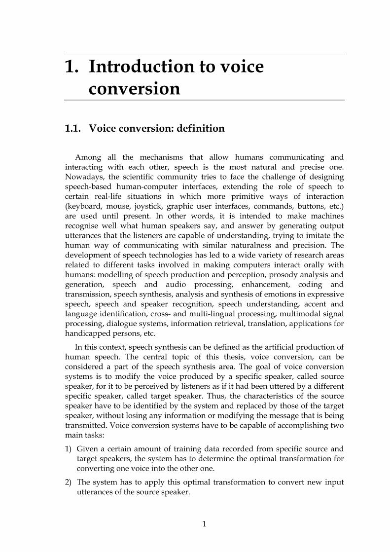
The main applications of voice conversion are related to the speech synthesis field. The aim of Text-to-Speech (TTS) synthesis systems is to convert words in written format into speech. The way of operating of a standard TTS system can be described as follows [Hua01]:
First, the input text, which may contain not only regular words but also numbers, dates, acronyms, proper names, foreign words, etc., has to be translated into a sequence of phonetic symbols.
Second, the so called prosody generation block attaches appropriate rhythm and intonation information to the phonetic sequence, according to the knowledge acquired during a previous training process.
Finally, the output speech waveform is generated following the phonetic and prosodic specifications provided by the previous blocks.
The block diagram of a generic TTS system is shown in figure 1.1.
Figure 1.1: block diagram of a TTS system.
At present, the waveform generation module of high-quality TTS systems is based on unit selection: the synthetic utterances are built by selecting appropriate speech segments from a pre-recorded database and concatenating them together. The physical attributes of the concatenated units are modified to match the desired intonation patterns and also to avoid audible discontinuities in the synthetic speech. Incorporating voice conversion technologies into TTS systems allows transforming the pre-recorded voice into any other target voice, so that it would not be necessary to record an entire database for each of the desired output voices. Avoiding multiple recordings and their associated post-processing is interesting because in general this is an expensive and time-consuming activity. Furthermore, it helps to reduce the amount of memory required by a multi-speaker synthesis system, increasing its portability and making easier to integrate it into mobile phones or small devices. Since the voice conversion functions can be trained from few minutes of audio and take up few amount of memory, it is possible to transmit and incorporate new voices to the synthesizer in an easy way.
Voice conversion systems have interesting applications in the entertainment industry: dubbing the voice of actors in different languages, synthesizing the voice of actors that are not alive or that have lost their voice to some extent, creating virtual clones of famous people for videogames, etc. In addition, voice
Text processing
Prosody generation
Waveform generationText
Speech signal
Intra-lingual and cross-lingual voice conversion using harmonic plus stochastic models
3
conversion systems can also be applied to create unknown target voices, so that a single TTS engine can generate multiple perceptually different voices for different characters in videogames, for instance, without increasing the memory requirements of the system.
Speech-to-speech translation technology is devoted to creating translating machines that serve as interpreters in multilingual conversations between two or more people speaking different languages. Such machines decompose the problem into three different subtasks: first, the utterances in the source language are converted into text using speech recognition tools; then, machine translation techniques are applied to translate the text to the target language; finally, the translated sentences are spoken by a TTS system. In this situation, it is desirable that the listeners can easily identify the speaker whose utterances are being translated, so voice conversion systems can be applied to transform the standard voice of the TTS system into the voice contained in the speech signal at the input of the speech recogniser. One of the main problems of designing a voice conversion system for speech-to-speech translation is the fact that the source and target speakers do not speak the same language.
In a medical context, another application field is the design of speaking aids for people with speech impairments or hearing aids for specific hearing problems. Voice conversion may also help to improve the pronunciation of different phonemes spoken by children or students of foreign languages, letting them hear their own voice pronouncing the problematic sentences without errors.
From a scientific point of view, acquiring a high level of knowledge about speaker individuality would be very useful to make progress in other speech technologies like speaker-independent speech recognition, speaker recognition, very-low-bandwidth speech coding using an adequate parameterization of the speaker-dependent information, etc.
1.3. Speech signal and speaker individuality
The human physical mechanism for producing speech can be described as follows. The speaking process breaks out when the speaker pushes air from the lungs through the trachea. The airflow reaches the glottis, where the vocal cords can be open or closed. When producing unvoiced sounds such as, for instance, fricative consonants, the vocal cords remain open and the airflow crosses the larynx without obstacles. Instead, when the sounds being produced are voiced like vowels, the speaker closes the vocal cords, so the air pressure under the larynx gradually increases until the resistance of the vocal cords is not enough to restrain the airflow. Then, the airflow crosses the glottis and the pressure below decreases until the vocal cords are closed again. This phenomenon is repeated periodically, making the vocal cords vibrate. In any of the two cases, after having crossed the glottis, the airflow passes through the vocal tract,
Chapter 1. Introduction to voice conversion
4
composed of the pharynx, the nasal cavity and the oral cavity, whose shape is determined by physical articulators like the lips, the jaw, the tongue and the teeth. The speaker controls the position of all these articulators for producing specific phonemes.
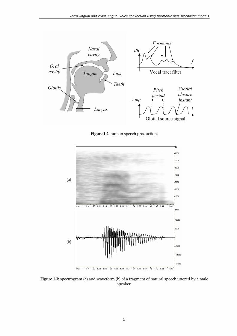
From a signal processing point of view, the speaking process can be described by the so called source-filter model, where the source signal represents the airflow coming from the glottis, and the physical vocal tract is represented by a filter that modifies the frequency-shape of the source signal. The speech production process is illustrated in figure 1.2. The glottal source signal that corresponds to voiced sounds looks like a train of pulses whose amplitude is proportional to the opening area of the vocal cords. Thus, the glottal closure instants are located at the zeros of the signal. The time between two consecutive glottal closure instants, which depends on the physical characteristics of the vocal cords, determines the fundamental frequency or pitch of the produced speech signal. The pitch frequency is usually represented by the symbol f0. Since the glottal source is quasi-periodic, it can be represented in the frequency domain by a set of sinusoids whose frequencies are integer multiples of the pitch, f0. The unvoiced sounds are characterized by a noise-like glottal source signal. The vocal tract filter shapes in frequency the glottal source signal according to the instantaneous position of the articulators, and therefore it is characterized by a number of time-varying resonances, called formants. In a steady state, each phoneme is characterized by a specific formant structure, so when a sequence of phonemes is uttered by the speaker, the physical articulators of the vocal tract make the formants move gradually from a steady position to the next.
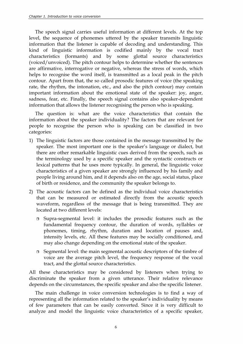
Thus, the speech signal perceived by listeners can be seen as the result of filtering the glottal source through the vocal tract. The spectrogram and the waveform of a real speech fragment are shown in figure 1.3. The unvoiced speech segments (first part of the signal in figure 1.3) have noise-like aspect in the time domain, whereas the voiced speech segments look like locally periodic waveforms. Therefore, the voiced segments are characterized in the frequency domain by the presence of harmonically-related signal components, whose intensity varies in frequency. The most powerful harmonics are those that coincide with the positions of the vocal tract formants. The magnitude spectrum of the speech signal is conditioned by the frequency response of the vocal tract, but also by the spectral characteristics of the glottal source signal, derived from the voiced/unvoiced property, the pitch frequency f0 and the shape of the glottal pulses.
Intra-lingual and cross-lingual voice conversion using harmonic plus stochastic models
5
Figure 1.2: human speech production.
(a)
(b)
Figure 1.3: spectrogram (a) and waveform (b) of a fragment of natural speech uttered by a male speaker.
Nasal cavity
Oral cavity Tongue Lips
Teeth Glottis
Larynx
Vocal tract filter
f
dB Formants
Glottal source signal
t
Amp.
Glottal closure instant
Pitch period
Chapter 1. Introduction to voice conversion
6
The speech signal carries useful information at different levels. At the top level, the sequence of phonemes uttered by the speaker transmits linguistic information that the listener is capable of decoding and understanding. This kind of linguistic information is codified mainly by the vocal tract characteristics (formants) and by some glottal source characteristics (voiced/unvoiced). The pitch contour helps to determine whether the sentences are affirmative, interrogative or negative, whereas the stress of words, which helps to recognise the word itself, is transmitted as a local peak in the pitch contour. Apart from that, the so called prosodic features of voice (the speaking rate, the rhythm, the intonation, etc., and also the pitch contour) may contain important information about the emotional state of the speaker: joy, anger, sadness, fear, etc. Finally, the speech signal contains also speaker-dependent information that allows the listener recognising the person who is speaking.
The question is: what are the voice characteristics that contain the information about the speaker individuality? The factors that are relevant for people to recognise the person who is speaking can be classified in two categories:
1) The linguistic factors are those contained in the message transmitted by the speaker. The most important one is the speaker’s language or dialect, but there are other remarkable linguistic cues derived from the speech, such as the terminology used by a specific speaker and the syntactic constructs or lexical patterns that he uses more typically. In general, the linguistic voice characteristics of a given speaker are strongly influenced by his family and people living around him, and it depends also on the age, social status, place of birth or residence, and the community the speaker belongs to.
2) The acoustic factors can be defined as the individual voice characteristics that can be measured or estimated directly from the acoustic speech waveform, regardless of the message that is being transmitted. They are located at two different levels:
Supra-segmental level: it includes the prosodic features such as the fundamental frequency contour, the duration of words, syllables or phonemes, timing, rhythm, duration and location of pauses and, intensity levels, etc. All these features may be socially conditioned, and may also change depending on the emotional state of the speaker.
Segmental level: the main segmental acoustic descriptors of the timbre of voice are the average pitch level, the frequency response of the vocal tract, and the glottal source characteristics.
All these characteristics may be considered by listeners when trying to discriminate the speaker from a given utterance. Their relative relevance depends on the circumstances, the specific speaker and also the specific listener.
The main challenge in voice conversion technologies is to find a way of representing all the information related to the speaker’s individuality by means of few parameters that can be easily converted. Since it is very difficult to analyze and model the linguistic voice characteristics of a specific speaker,
Intra-lingual and cross-lingual voice conversion using harmonic plus stochastic models
7
current voice conversion systems are addressed mainly to the acoustic features of voice. Indeed, a vast majority of them focus only on the segmental level. For this reason, the process of transforming only the acoustic characteristics of voice will be also called voice conversion throughout this dissertation.
1.4. Objectives of the thesis
The general objective of this thesis is to research into voice conversion systems and methods in order to improve their quality and versatility.
The first specific objective of the thesis is to design new spectral conversion methods that succeed at converting the source voices into the target voices without degrading significantly the quality of the manipulated signals, and implement the consequent voice conversion system.
The second specific objective is to create a voice conversion system capable of estimating adequate voice conversion functions in all possible training scenarios:
Intra-lingual scenario with parallel corpus available: the same training sentences are uttered by both the source and target speakers in the same language, so the correspondence between phonetic characteristics is easy to establish.
General intra-lingual scenario: the training sentences of the source and target speakers are uttered in the same language but are not necessarily the same.
Cross-lingual scenario: the source and target training sentences are not the same and are uttered in a different language. In this case, studies will be carried out in English and Spanish.
The third objective consists of integrating the resulting voice conversion system into a TTS system, so that it can operate not only as a conversion device whose input is a given speech signal and whose output is the converted voice, but also as a stand-alone TTS system that generates different converted voices from a single synthesis database.
The degree of fulfilment of the described objectives will be determined by means of perceptual tests: the similarity between converted and target voices and the quality of the converted speech will be rated by real listeners, so that the final performance scores are reliable and give an idea of the impact that the resulting system can have in the real world. The resulting voice conversion system is to be used for real-life applications, so a very important point is that the quality of the synthetic converted speech has to be satisfactory for the listeners. The research will be addressed to achieve high similarity scores between converted and target voices, but a higher priority will be given to the quality scores.
Chapter 1. Introduction to voice conversion
8
It has to be clarified that in this dissertation the definition of voice conversion will be restricted to the transformation of the acoustic characteristics of voice. Moreover, the transformation of prosodic contours is also out of the scope of this thesis. Only the mean pitch level of speakers will be adapted.
1.5. Thesis overview
The rest of the dissertation is organized as follows.
In chapter 2, the current state of the art of voice conversion technologies is critically analyzed, determining the problems that remain still unsolved and the limitations of existing techniques.
Chapter 3 is devoted to the design of a suitable speech model that allows all kind of prosodic and spectral manipulations of the speech signal. The main contributions and novelties contained in chapter 3 are the following:
A new method for time-scale modification of speech signals analyzed at a constant frame rate using a harmonic plus stochastic model.
A new method for estimating the linear-in-frequency phase term of a given set of harmonic sinusoids, and its application to calculate phase envelopes.
A new method for pitch-scale modification of speech signals analyzed at a constant frame rate using a harmonic plus stochastic model.
A new method for eliminating the phase mismatches at the boundaries of speech units to be concatenated.
In chapter 4, a baseline voice conversion system is built using the model described in chapter 3 and state-of-the-art transformation techniques. After that, new techniques for converting spectral envelopes are proposed. The contributions presented in this chapter are:
The implementation details of a voice conversion system based on state-of-the-art techniques using a harmonic plus stochastic model. The harmonic spectral envelope is parameterized and converted by means of linear transformations, and the stochastic envelope is predicted from the harmonic one in voiced segments, whereas in unvoiced segments it is left unmodified. A simple pitch level adaptation between speakers is applied.
A new method for spectral envelope conversion, called Weighted Frequency Warping, which is a combination between statistical methods and frequency warping transformations. It gives very good results in terms of conversion-quality balance.
Intra-lingual and cross-lingual voice conversion using harmonic plus stochastic models
9
Two methods for calculating optimal piecewise linear frequency warping functions automatically. One of them results to fit very well with the new spectral envelope conversion method mentioned above.
Chapter 5 presents a new method for aligning speech frames from different speakers when only non-parallel sentences are available for training the voice conversion system. Thus, it contains two main novelties:
A new iterative method for frame alignment.
Evaluation of a complete voice conversion system based on Weighted Frequency Warping and the proposed alignment method in intra-lingual and cross-lingual conditions.
Chapter 6 is devoted to the design of a multi-speaker TTS system using the voice conversion techniques presented in previous chapters. The main contributions of this chapter are the results and discussion of the system evaluation.
Finally, in chapter 7 the main conclusions of this dissertation are summarized and some possible research lines for future work are proposed.
Appendix A contains a detailed description of Ogmios, the UPC TTS synthesis system, which is used for the experiments concerning synthetic voices in chapters 3 and 6. Appendix B describes the recording databases used for the voice conversion tests throughout the thesis.

Chapter 1. Introduction to voice conversion
10
11
2. State of the art of voice conversion technologies
Voice conversion systems try to capture the speaker’s individuality by means of few parameters, so that it can be easily converted. Although a complete voice conversion system should transform all types of speaker-dependent characteristics of speech, as it has been stated in chapter 1, current voice conversion systems are focused only on the acoustic features of voice. Moreover, a vast majority of them are focused only on segmental-level features.
Research studies on the relationship between voice individuality and certain acoustic features have a relatively long history. For instance, Matsumoto et al. investigated contributions of pitch, formant frequencies, spectral envelope and other acoustic parameters [Mat73]. They concluded that f0 was the most important descriptor for individuality, followed by formant frequencies, f0 fluctuations and spectral tilt. Sato found that the average speech spectrum was useful for gender discrimination [Sat74]. Itoh and Saito [Ito82] showed that the spectral envelope had the greatest influence on individuality, followed by f0 and temporal structure. Furui studied the relationship between psychological and physical distances among speakers [Fur86], and reported that the long-term average spectrum smoothed by cepstrum coefficients showed the highest correlation, followed by averaged f0. In particular, the 2.5-3.5 KHz frequency range was found to have the greatest contribution to individuality. Taking all these previous studies into account, Kuwabara and Sagisaka stated that voice individuality is an amalgam of many parameters, whose relative relevance can differ from speaker to speaker and thus depends on the nature of the speech material under study [Kuw95]. According to the conclusions of those studies, the voice conversion systems found in the literature are addressed in general to transforming the short-time spectral envelopes and the pitch level of the involved speakers, and some of them are also extended to supra-segmental features like pitch contours.
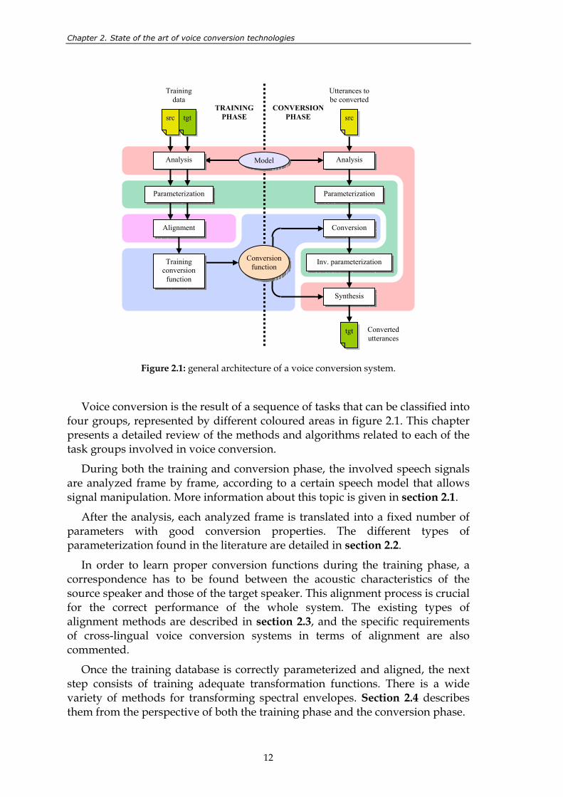
The general architecture of a voice conversion system is shown in figure 2.1. As it can be observed, the voice conversion process can be decomposed into two phases: the training phase and the conversion phase. During the training phase, the function for transforming the voice characteristics of the source speaker into those of the target speaker is learnt from a training database that contains recorded speech utterances. During the conversion phase, the system applies the already trained function to transforming new input utterances of the source speaker.
Chapter 2. State of the art of voice conversion technologies
12
Figure 2.1: general architecture of a voice conversion system.
Voice conversion is the result of a sequence of tasks that can be classified into four groups, represented by different coloured areas in figure 2.1. This chapter presents a detailed review of the methods and algorithms related to each of the task groups involved in voice conversion.
During both the training and conversion phase, the involved speech signals are analyzed frame by frame, according to a certain speech model that allows signal manipulation. More information about this topic is given in section 2.1.
After the analysis, each analyzed frame is translated into a fixed number of parameters with good conversion properties. The different types of parameterization found in the literature are detailed in section 2.2.
In order to learn proper conversion functions during the training phase, a correspondence has to be found between the acoustic characteristics of the source speaker and those of the target speaker. This alignment process is crucial for the correct performance of the whole system. The existing types of alignment methods are described in section 2.3, and the specific requirements of cross-lingual voice conversion systems in terms of alignment are also commented.
Once the training database is correctly parameterized and aligned, the next step consists of training adequate transformation functions. There is a wide variety of methods for transforming spectral envelopes. Section 2.4 describes them from the perspective of both the training phase and the conversion phase.
Converted utterances
Analysis
Parameterization
Alignment
Training conversion
function
Analysis
Parameterization
Conversion
Synthesis
tgt
Inv. parameterization
TRAINING PHASE
CONVERSION PHASE src tgt
Training data
Utterances to be converted
src
Model
Conversion function
Intra-lingual and cross-lingual voice conversion using harmonic plus stochastic models
13
Apart from spectral envelopes, one of the most important physical characteristics to be converted is the pitch of speakers. Most of the existing systems perform a simple mean-pitch-level adaptation. Nevertheless, some works dealing with pitch contours and more general prosodic transformations (related to supra-segmental aspects of voice) can also be found in the literature. Section 2.5 contains a brief review of pitch transformation techniques.
Finally, in section 2.6 the conclusions of this bibliographic study are summarized.
2.1. The analysis/reconstruction framework
One of the most important design characteristics of a voice conversion system is the speech model used to analyze the input signals and reconstruct the modified signals. A good speech model for voice conversion has the following characteristics:
First of all, it allows reconstructing the signal from the model parameters (copy synthesis) with high fidelity, so that the reconstructed signal and the original signal are almost indistinguishable.
It provides procedures for modifying the prosodic characteristics of speech (pitch, duration and intensity) without introducing artifacts.
The first two characteristics mean that the chosen model is suitable for synthesis purposes, but there is a third condition:
The model has to allow flexible spectral modifications that do not degrade the quality of the synthesized speech.
The relationship between the voice conversion system and its underlying synthesis system is very close, because a correct interaction between them is necessary when transforming prosodic features like the pitch. Furthermore, artifacts coming from the analysis-synthesis process are still present in the converted signal.
One of the most popular synthesis techniques is TD-PSOLA [Mou90], which provides high-quality synthesized speech with artifact-free prosodic modifications. However, it assumes no model for the speech signal. Instead, it operates directly on the samples in the time-domain, so it cannot be applied to voice conversion. Instead, some other variants of the PSOLA technique have been successfully used for voice conversion, like LP-PSOLA or FD-PSOLA [Mou95]. Some examples can be found in [Val92, Sün05, Tur06, Dux06a].
Models based on a sinusoidal decomposition of speech [Mca86a, Qua92, Rod02] are very suitable for voice conversion, because they provide a high degree of flexibility to manipulate the parameterized signal. Harmonic models are a particular case of sinusoidal models. Some voice conversion systems using sinusoidal and harmonic models can be found in [Kai01, Ye06, Shu06]. In
Chapter 2. State of the art of voice conversion technologies
14
[Sty96], the harmonics plus noise model (HNM, based on the decomposition of the speech signal into a harmonic component and a noise-like component) was successfully applied to building a voice conversion system [Sty98]. In order to avoid problems related to the phase, most of the sinusoidal and hybrid systems operate in a pitch-synchronous way, using PSOLA-like methods for prosodic manipulation.
The STRAIGHT model [Kaw97] is also useful for conversion purposes. STRAIGHT uses pitch-adaptive spectral analysis combined with a surface reconstruction method in the time-frequency region, and an excitation source design based on phase manipulation. It allows very high manipulation factors for pitch and duration, without significant quality degradation. This kind of representation is adequate to interpolate spectral envelopes and to extract parameters like the cepstral coefficients. The STRAIGHT representation was used in [Tod01, Tod05, Tod06, Oht07a, Oht07b].
Recently, more complex models of speech describing both the glottal source and the vocal tract have reached satisfactory performance in terms of signal manipulation [Vin07, Per05], and it is expected that the extension of current voice conversion techniques to such kind of models will lead to significant improvements in this field.
2.2. Parameterization
All the voice conversion systems found in the literature analyze, transform and regenerate each signal frame individually. There are three main reasons for parameterizing the speech frames before training and applying voice conversion functions:
The identity of a speaker is well represented by some kind of parameters.
It is extremely difficult to convert voices directly from the data given by the analysis (signal periods, short-time spectrum samples, amplitudes + frequencies + phases, etc.). Converting low-dimensional vectors is easier.
The parameters used in voice conversion tasks have in general good interpolation properties.
The most typical types of parameterizations used in voice conversion tasks are the following:
Parameters related to formants, like formant frequencies, bandwidths and intensity [Abe88, Miz94, Gut98, Gut01, Ren04, Shu06].
All types of cepstral coefficients (CC): discrete cepstrum [Sty96], MFCC [Tod05, Sty98], LPC-cepstrum [Lee07]. The main reason for choosing such coefficients is that they have been widely used in other areas of speech technology like speech or speaker recognition, with very good results. Furthermore, they provide a reliable measure of acoustic distance
Intra-lingual and cross-lingual voice conversion using harmonic plus stochastic models
15
between different frames, which is an important property for alignment tasks.
Line spectral frequencies (LSF) [Ars99, Kai01, Ye06, Sün06, Dux06b], which are a special representation of all-pole filters. LSFs are reported to have very interesting properties for voice conversion tasks.
In some cases, the spectral samples are directly used for voice conversion instead of more handy parameterizations. This is adequate when the system applies transformation functions based on frequency warping of spectrums [Val92, Sün03a].
Studies on the convenience of different parameterizations [Kai01, Ye04a] conclude that LSF are advantageous with respect to other spectral representations for several reasons:
They are a good representation of the formant structure.
They have better interpolation properties.
A perturbation in one of the coefficients affects only a small portion of the spectrum.
The use of LSF coefficients is very common in recent voice conversion systems.
2.3. Alignment
Voice conversion systems are capable of learning transformation functions from the training data of the source and target speakers. In order to map the source speaker’s acoustic space to the target speaker’s acoustic space, it is necessary to have a previous knowledge about the source-target correspondence between different training units. The process in which this correspondence is established is called alignment. Several alignment strategies can be adopted, depending on the requirements of the spectral envelope transformation method applied by the system. They can be divided in three groups.
2.3.1. Alignment of acoustic classes
In some voice conversion systems, like for instance those based on mapping codebooks or frequency-warping functions [Ars98, Sün03a], the input source vectors belonging to different acoustic classes are transformed in a different way. Thus, in order to train class-dependent functions, a correspondence has to be found between the acoustic classes of the source speaker and those of the target speaker. Ideally, each class represents the characteristics of a certain phoneme or phoneme group.
Chapter 2. State of the art of voice conversion technologies
16
In [Ars98] the states of hidden Markov models are interpreted as acoustic classes. The same speaker-independent model is used to segment the source and target speaker’s utterances, so the correspondence between them is automatically established. In [Sün03a] the classification is performed by means of clustering techniques, and the source-to-target correspondence is determined using minimum-distance criteria.
2.3.2. Frame-to-frame alignment
A vast majority of voice conversion systems found in the literature learn vector-transformation functions from a set of paired parameter vectors (each vector contains the parameters of one speech frame). If a parallel training corpus is available, it is very simple to find the source-to-target correspondence at frame level. A parallel corpus is obtained when exactly the same training sentences are uttered by both the source speaker and the target speaker. The use of parallel training corpora guarantees that the phonetic sequence is the same for both speakers, so the alignment process is simplified. In this case, the most preferred frame-alignment technique is dynamic time-warping (DTW), almost standard in voice conversion systems [Abe88, Sty98, Kai01, Sün05, Tod05]. The main disadvantage of DTW is that the optimal source-target pairs are determined by searching the path of minimal global distortion without taking into account the differences between speakers. Stylianou proposes an improved alignment that consists of a first alignment based on DTW, an initial estimate of the voice conversion function, and then a second DTW-realignment of converted-target vectors, so that a much more accurate correspondence between frames is found [Sty07].
An alternative method based on hidden Markov models (HMM) has been also proposed for parallel training sentences whose orthography and phonetic transcription are known. First, all the sentences are segmented using speaker-dependent models. Then, the boundaries of the phonemes or sub-phonemes are taken as anchor points, and linear time-warping [Dux06b] or dynamic time-warping [Ye06] is used inside the units to establish the correspondence between source and target vectors. A high-accuracy alignment is obtained by means of this procedure, but it must be taken into account that training accurate HMMs requires enough training data from each of the speakers.
In a very recent work [Nan07], statistical methods have been also applied to optimize the spectral conversion function and the time-sequence matching of vectors simultaneously, using maximum likelihood criteria. The results reported point that such a statistical method outperforms typical systems in which alignment and training are separate processes.
In a realistic voice conversion application, only non-parallel corpora may be available during the training phase. Four different alignment methods have been used in this situation:
Intra-lingual and cross-lingual voice conversion using harmonic plus stochastic models
17
Class mapping [Sün04]. The source and target vectors are classified separately in clusters. A first mapping is established between each source acoustic class and one of the target acoustic classes by comparing the associated vocal-tract-normalized centroids. Then, all the vectors inside each class are mean-normalized and finally the frame alignment is performed by finding the nearest neighbour of each source vector in the corresponding target class.
Dynamic programming [Sün06a]. Given a set of N source vectors sk, the dynamic programming technique is used to find the sequence of N target vectors tk that minimizes the cost function calculated as follows:
( ) ( ) ( ) ( )∑∑ = −=−+=
N
k kkN
k kkk ddC2 11
,1, tttst αα (2.1)
The underlying idea is similar to that of unit selection: the global cost function C takes into account the source-target cost but also the target-target concatenation cost. The function d(·) represents the acoustic distance between two vectors, and the factor α is empirically adjusted depending on the relevance of each kind of distance. This alignment technique is reported to outperform the previous one, and it allows building a text-independent and language-independent system, because the correspondence between frames is obtained using acoustic criteria only. However, it has two drawbacks: (a) it is very time-consuming, and (b) increasing the size of the training database implies worsening the conversion scores, since the optimal sequence tk is closer to sk when there are more frames available for selection.
Speech recognition [Ye04b]. A speech recognizer operating with speaker-independent HMMs is used to label all the source and target frames with a state index. Given the state sequence of one speaker, the alignment procedure consists of finding longest matching sub-sequences from the other speaker until all the frames are paired.
Unit selection using a TTS system [EnN05, Dux06]. In some applications like the customization of a text-to-speech synthesizer, a huge database of speech from the source speaker is available, so the TTS system can be used for generating the same sentences that have been recorded from the target speaker. Given that a parallel training corpus is now available, the parameter vectors can be aligned by DTW or HMM. The main disadvantage of this method is that it can be applied only when there are enough data from the source speaker to build a TTS system. This strategy is incompatible with cross-lingual applications.
2.3.3. No alignment
Some of the systems found in the literature do not actually require an alignment method. Instead, a certain acoustic model is estimated from the
Chapter 2. State of the art of voice conversion technologies
18
training data of one of the speakers and the optimal transformation function is calculated using the information contained in the model itself.
In [Ye06], acoustic hidden Markov models are trained from the training parameter vectors of the target speaker, and a probabilistic voice transformation function is statistically estimated in such way that the transformed source vectors give maximum likelihood with respect to the model. The transformation function used in this work is based on a gaussian mixture model of the source vector space.
Some other approaches are based on adaptation of models: an already trained transformation function between speakers A and B is adapted to the acoustic data of a different target speaker C. Two different adaptation techniques have been proposed for voice conversion: maximum-a-posteriori (MAP) adaptation [Lee06] and maximum-likelihood stochastic transformations (MLST) [Mou06]. The MLST technique allows also adapting the conversion function to a different source speaker.
Before concluding, the increasing prominence of HMM-based systems in the speech synthesis field has to be emphasized [Mas96]. Given one input text and one HMM already trained, such systems are capable of generating an optimal output sequence of parameter vectors from which the synthetic utterance can be reconstructed. HMM-based speech synthesis systems have successfully used adaptation techniques like MAP or MLLR (maximum-likelihood linear regression) to synthesize speech with different voices: the initial HMM is estimated from the training data of the source speaker, and then it is adapted to maximize the likelihood of the target speaker’s training vectors with respect to the modified HMM [Mas97, Tam98]. The adapted model can be directly used for synthesizing speech with the target voice. This is a conceptually different formulation of the voice conversion problem, restricted to the domain of TTS systems. The main problem associated to this promising technology is that at present, in spite of the recent improvements [Zen07], the quality of the synthetic speech obtained through HMMs is still limited by the statistical synthesis procedure itself, and the same occurs when synthesizing speech from adapted HMMs. This is the reason why typical voice conversion systems are usually combined with corpus-based speech synthesis systems, whose associated quality scores are closer to those of natural speech.
2.3.4. Requirements of cross-lingual voice conversion
Cross-lingual voice conversion is the most extreme situation in terms of alignment. Voice conversion systems dealing with different languages have some special requirements because the utterances available for training are characterized by different phoneme sets. Obviously, the main difference between intra-lingual and cross-lingual alignment is that it is not possible to obtain parallel corpora from utterances in different languages, so the most
Intra-lingual and cross-lingual voice conversion using harmonic plus stochastic models
19
popular alignment strategies are not valid anymore. On the other hand, it can be remarked that training cross-lingual voice conversion functions would not be problematic at all if the alignment problem was solved. Despite the recent appearance of some cross-lingual applications for voice conversion like speech-to-speech translation, few works on cross-lingual voice conversion can be found in the literature.
As explained before, systems using adaptation techniques (MAP, MLLR, etc.) do not need an explicit alignment between source and target vectors or acoustic classes. Since the adaptation of acoustic models is a statistical procedure, using this kind of systems makes cross-lingual voice conversion possible [Mou06, Lee06, Lat06].
Systems requiring alignment can be trained in cross-lingual conditions when at least one of the speakers is bilingual: the transformation function for acoustic vectors can be estimated using conventional methods from a parallel corpus recorded in the language that both speakers have in common (in fact, it is enough if only one of them is bilingual). In the conversion phase, this acoustic function can be applied to transforming the voice of the source speaker without worrying about the language. This strategy was successfully adopted in [Abe90, Mas01, Dux06b]. The main disadvantage of this simple approach is that it is difficult to find bilingual speakers for every pair of languages.
Among the techniques proposed for aligning frames when only non-parallel corpora are available, only those that perform the alignment following exclusively acoustic criteria are compatible with cross-lingual voice conversion [Sün03b, Sün06b]. The rest of techniques are based on intra-lingual HMMs and TTSs, and although theoretically they could be extended to a cross-lingual context, it has not been done yet. An adequate alignment technique based exclusively on acoustic features is desirable for several reasons:
The problem of finding bilingual or multilingual speakers for recording parallel corpora is avoided.
It transforms non-parallel training corpora into parallel corpora compatible with almost all the voice conversion systems.
Since it does not use linguistic information of any kind, it allows text-independent and language-independent voice conversion.
2.4. Spectral envelope conversion methods
The transformation of spectral envelopes is the central task of a voice conversion system. A vast majority of the publications on voice conversion are related to this task. A lot of different techniques have been proposed during the last twenty years, since the voice conversion problem was stated in 1988. Despite the diversity of methods, they can be classified in six groups, depending on the type of transformation that they apply. A detailed
Chapter 2. State of the art of voice conversion technologies
20
explanation of the existing spectral conversion methods and algorithms is presented in the following subsections.
2.4.1. Methods based on mapping codebooks
The first work on voice conversion was carried out by Abe et al. in 1988 [Abe88]. The system is based on vector quantization (VQ) and mapping codebooks. The training phase consists of the following steps:
1) The source and target speakers pronounce a learning word set. All the words are vector-quantized frame by frame.
2) The correspondence between vectors of the same words from the two speakers is determined using DTW. The correspondences are accumulated as histograms.
3) Using each histogram as a weighting function, the mapping codebook is defined as a linear combination of the target speaker’s vectors.
4) Steps 2 and 3 are repeated to refine the mapping codebook.
The vectors contain acoustic features like formant frequencies and bandwidths, spectral tilt, glottal waveform, etc. In the conversion phase, the source speaker’s input utterance is LPC-analyzed and the spectrum parameters are vector-quantized using the source speaker’s own codebook. Then, they are decoded using the source-target mapping codebooks.
In [Shi91], the concept of fuzzy vector-quantization and fuzzy mapping is applied to improve the previous system. Each source vector is represented as a weighted linear combination of all the codewords. Every correspondence between the two sets of codewords is taken into account when converting the source vectors.
In the voice conversion system proposed by Mizuno and Abe in 1994 [Miz94], the codewords of a one-to-one mapping codebook are inspected to extract their formant frequencies, formant bandwidths and spectral tilt. The correspondence between the formants of each pair of source and target codewords is established manually, and the formant frequency shift values and tilt shift values are stored as transformation rules. In the conversion phase, the input source speech is vector quantized by frames using the codebook of the source speaker. The LPC poles whose characteristics are closer to the reference formants of the dominant codeword are chosen as current formants, and the associated rules are applied to them. The spectral tilt is copied directly from the codeword. The modification of all the parameters is performed simultaneously using an algorithm that minimizes the spectral distortion. The authors concluded that the listeners preferred this system rather than the classical VQ system, because it guaranteed a higher speech quality after the modification.
Intra-lingual and cross-lingual voice conversion using harmonic plus stochastic models
21
In 1999, Arslan proposed a new codebook-based conversion method: STASC (speaker transformation algorithm using segmental codebooks) [Ars99]. In this case, a transfer function H(w) is calculated for each frame so that the target frame is obtained as
( ) ( ) ( ) [ ] ( ) ( )wYFTnywXwHwY 1Re, −=⋅= (2.2)
The speech frames are classified by phonemes or by HMM states, and the average LSF vector of each cluster is calculated for the source speaker, Si, and for the target speaker, Ti. These vectors are taken as entries of a one-to-one mapping codebook. Given a source LSF input vector x, the distance from x to each of the codewords Si, called di, is calculated as
∑ =
−+− −⋅−−=
p
k ikkkkkkid1
111 ,min Sxxxxx (2.3)
The sub index k denotes the kth vector element. The length of the vectors is p. Since the presence of a formant is characterized by two close line spectral frequencies, the distance function includes a weighting factor that emphasizes the contribution of these lines. Then, a weight vi is assigned to each of the codebook words Si, obtained as
∑ −
−
=
j
d
d
i j
i
eev γ
γ
(2.4)
for a certain optimal γ whose calculation details are omitted here. The converted vector F(x) is then calculated as follows:
( ) ∑=i
iivF Tx (2.5)
The transfer function for the current frame is given by the all-pole filters associated to the LSF vectors x and F(x), Vx(w) and VF(x)(w) respectively.
( ) ( ) ( )wVwVwH xxF )(= (2.6)
As explained afterwards, the author proposed also to modify the LPC excitation signal and other features related to prosodic aspects of the speech.
An evolution of the STASC method was presented by Turk and Arslan in [Tur06]. First, some refinements were made in the codebooks to eliminate the source and target classes that had been matched in the alignment step but were significantly different (i.e. accent reasons). A spectral equalization procedure was also used to cope with the problem of the different recording environments between the source and target speakers. Finally, the use of a pre-emphasis filter was discussed in order to make the system more robust to small variations in the speech signal.
One of the most novel approaches based on vector-quantization was the one developed by Salor and Demirekler in 2006 [Sal06]. Their system is trained using a parallel corpus: the sentences are automatically segmented into phones using HMMs, and DTW is used inside each phone to obtain the frame pairs. Using a LSF parameterization, the frames of both speakers are vector-quantized
Chapter 2. State of the art of voice conversion technologies
22
and a codebook is obtained for each speaker: Sii=1..L and Tjj=1..L. From the sequence of training vectors, an L×L histogram matrix H is obtained. H(i, j) shows how many times the pair Si, Tj was found in the aligned vector-quantized training corpus. Another L×L matrix P is obtained for the target speaker, in which P(i, j) indicates the transition probability from the ith class to the jth class, based on the number of occurrences found in the training data. Given a sentence from the source speaker to be converted, it is firstly translated into N vector-quantized frames. Then, the N×L histogram matrix H(sen) associated to the whole sentence is built: the kth row of H(sen) is copied from the row of H associated with the class assigned to the kth frame, representing the probability of each target class to be paired with it. Finally, the dynamic programming procedure is used to find the best trajectory from the first row of H(sen) to the last one, obtaining the N-length sequence of target classes that maximizes the probability function given by the product of their individual probabilities in H(sen) and the transition probabilities between them, provided by the matrix P. The converted signal is synthesized following the selected sequence of target codewords.
2.4.2. Methods based on frequency-warping functions
The dynamic frequency warping technique was first introduced by Valbret et al. in [Val92]. Given a pair of spectra X(w) and Y(w), modelled by them log-spectral samples, this technique finds the frequency warping function w’(w) so that the spectral distance between X(w’(w)) and Y(w) is minimized. In practice, the warping function is calculated as a set of frequency bin pairs. In order to eliminate the effect of the glottal source, the spectral tilt is estimated and eliminated from X and Y before finding the optimal path. As the warping function is different for different phonemes, a vector-quantization procedure is applied to partition the acoustic space and then an independent warping function is defined for each class. During the conversion step, the warping function of the most suitable class is applied to the log-spectrum of the source speaker. The spectral tilt is also modified.
In [Sün03a], the acoustic space of the source and target speakers is divided into classes, and a correspondence is found between every source class and one target class. Different types of frequency-warping functions for vocal tract length normalization (VTLN) with one or more parameters are studied and compared. A smoothing technique is applied to the parameters of the warping functions of consecutive frames in order to avoid the artifacts caused by the discontinuities between different classes. The quality of the synthetic converted speech is reported to be very high, but the identity of the target speaker is not completely captured by this method.
Rentzos et al. proposed to apply frequency warping functions combined with HMMs of the formant trajectories [Ren04]. Prior to training the system, speaker-dependent HMMs of MFCCs are used to estimate the phoneme
Intra-lingual and cross-lingual voice conversion using harmonic plus stochastic models
23
boundaries by forced-alignment segmentation. The formant candidates associated to each HMM state are obtained by means of an LPC analysis and are modelled using another HMM whose associated feature vectors contain the frequency, bandwidth and intensity of the formants. This results in a two-dimensional HMM that is used to determine the formant trajectories, discarding the poles that do not represent real formants. The equation for voice conversion at frame t is expressed as
[ ] ( ) ( ) ( )[ ]twtwtwXtwtwY ,,,,, ∗∗⋅= βαγ (2.7)
The frequency warping function includes the mapping functions for both the formant frequency α(w,t) and bandwidth β(w,t), defined by sub-bands, and γ maps the spectral magnitude between the source and target speakers. Finally, the converted spectrum is translated into the converted LPC coefficients.
Recently, a very simple approach based on mapping formants was presented [Shu06]. The training step consists of selecting one or more key speech frames from the source and target speakers that can be considered equivalent in terms of acoustic content: phoneme, context, etc. The frames with most stable formants are preferred. For example, the central frames of phoneme /e/ are a good choice. The formants are extracted from the source and target key frames, and a piecewise linear warping function is defined by the paired frequency points, including (0, 0) and (π, π). In the experiments, a single warping function is used for all the frames, and a filter is included to compensate for the inter-speaker differences in the frequency distribution of the energy. The main advantage of this system is that the perceptual speech quality is almost unaltered, but obviously the identity conversion scores are low.
More types of non-linear frequency warping functions are investigated in [Pri06], obtaining similar conclusions with regard to the converted-to-target similarity and the quality of the synthetic speech.
2.4.3. Methods based on speaker interpolation
The idea of speaker interpolation was originally proposed by Iwahashi and Sagisaka in 1994 [Iwa94, Iwa95]. The authors state that the parameter vectors that characterize the spectral envelope of a generic target speaker can be obtained by a linear combination of parameter vectors obtained from a set of N different pre-stored speakers.
∑ ==
N
i ikik w1
xy (2.8)
Here, xik represents the vector xk obtained from the ith speaker. The weighting factors are estimated by minimizing the cepstral distance between the converted and target spectra.
Chapter 2. State of the art of voice conversion technologies
24
2.4.4. Methods based on neural networks
Neural networks have been also used for voice conversion purposes. Fewer details are given about this kind of techniques, because they did not reach an important impact, due to the almost simultaneous birth of GMM-based systems, whose performance really made a breakthrough in voice conversion technologies.
In [Nar95], artificial neural networks are used to learn a transformation function between the three first formants of the source speaker and those of the target speaker. The waveform is regenerated by a formant synthesizer.
A comparative study presented by Baudoin and Stylianou in 1996 [Bau96] shows that the performance of such systems is worse than that of GMM-based systems, which were born approximately at the same time.
In [Wat02], a three-layer radial basis function (RBF) network is used to convert the LPC spectral envelopes. The input vector x is applied to all the RBFs in the hidden layer. Each of them generates a radially symmetric response:
( ) ( )2
21
2exp iii
h cxx −−=σ
(2.9)
The kth element of the output vector y is obtained by the network by computing the following linearly weighted summation:
( ) ( )∑=i
kiik wh xxy (2.10)
In order to simplify the training, the centroids ci are chosen by applying the k-means algorithm to the source training vectors, and σi is forced to take the value ||ci||2. The weight coefficients are adjusted to minimize the least square error of the transformation for the training data.
2.4.5. Methods based on probabilistic linear transformations
One of the methods proposed in [Val92] is based on the concept of linear multivariate regression. The training speech frames of the source speaker are LPC-analyzed and vector-quantized into Q classes. For each of the classes, a transformation matrix is calculated as follows. First, the mean is subtracted from all the source vectors inside each class. Let Cq(s) be the matrix whose columns are the mean-normalized source vectors inside the qth class, and Cq(t) the matrix given by their aligned mean-normalized target vectors. Then, a transformation matrix Tq is calculated by finding the solution of the following least squares problem:
)()( sqq
tq CTC ⋅= (2.11)
Intra-lingual and cross-lingual voice conversion using harmonic plus stochastic models
25
During the conversion phase, the speech frames are vector-quantized and the mean vector and the transformation matrix of the assigned class are used to convert the spectral envelope. This method based on linear transformations is reported to provide a high degree of similarity between converted and target voices, but produces some audible distortions.
The use of statistical methods for converting spectral envelopes led to one of the most important advances in the voice conversion field. The most important drawback of the systems based on vector-quantization is the appearance of discontinuities in the transformation function near the transitions between classes. This problem is solved by dividing the acoustic space into overlapping classes, so that all the input vectors have a certain probability of belonging to each of the acoustic classes. In the system proposed by Stylianou [Sty96, Sty98], a gaussian mixture model (GMM) is fitted to the training acoustic vectors of the source speaker by means of the expectation-maximization (EM) algorithm.
( ) ( )∑=i
iii Np Σµxx ,;α (2.12)
N(x; µi, Σi) is a gaussian vector distribution defined by the mean vector µi and the covariance matrix Σi, and αi is the weight assigned to the ith gaussian component of the model. The proposed conversion function is given by the following expression:
( ) ( )[ ]∑ −+= −
iiiiiipF µxΣΓvxx 1)( (2.13)
where pi(x) denotes the probability that x belongs to the ith gaussian component. The vectors vi and matrices Γi are calculated during the training phase by minimizing the least squares error given by the distance between the transformed vectors F(xk) and the corresponding aligned target vectors yk, taken from a parallel corpus. The feature vectors contain discrete cepstral coefficients extracted from the amplitudes of the harmonic sinusoids found in the voiced frames. A noisy component is also extracted from all the frames, but its transformation is performed by two different corrective filters, one for the unvoiced frames and other for the aperiodic component of the voiced frames. The shape of the filters is trained by dividing the average noise periodogram of the target speaker by that of the source speaker.
In [Kai01] the aligned source and target LSF vectors are concatenated together and a joint GMM is trained from the resulting training vectors. The parameters of the gaussian components of such joint model, αi, µi, Σi, provide enough data to obtain the following conversion function:
( ) ( )[ ]∑ −+=−
i
xi
xxi
yxi
yi
xipF µxΣΣµxx 1)( ,
=
= yy
iyxi
xyi
xxi
iyi
xi
i ΣΣΣΣ
Σµµ
µ (2.14)
In this case, the probability pix(x) refers to the model defined by αi, µix, Σixx. At present, the described spectral envelope conversion method has become almost a standard, because it outperforms all the previous techniques in terms of balance between quality and conversion degree. The soft acoustic classification
Chapter 2. State of the art of voice conversion technologies
26
based on GMMs avoids the appearance of typical artifacts caused by the discontinuities in the transformation function. However, it was reported that the converted speech signal suffered from a certain over-smoothing effect that degraded the quality as well. Some authors tried to solve this new problem.
Since the quality of a frequency-warped spectrum remains high compared to that of unmodified speech, Toda et al. [Tod01] had de idea of combining the output of the GMM-based system and the DFW-based system. Given a source spectrum X(w) and its two converted spectra Ygmm(w) and Ydfw(w), the combined solution can be calculated by the following expression:
( ) ( ) ( ) ( ) ( )( ) ( ) 10,logloglogexp ≤≤−+= wwYwYwwYwY dfwgmmdfw γγ (2.15)
The weighting function proposed, γ(w), is linear in frequency. When using the described method, the speech quality is found to be much higher than in GMM-only systems, but there is a small decay in the conversion scores.
Another solution for the over-smoothing problem, proposed in [Che03], consists of using the probabilities given by the GMM to build a different transformation function, based on the concept of maximum-a-posteriori adaptation:
( )( )∑ −+=i
xi
yi
xipF µµxxx)( (2.16)
The mean target vectors are obtained by the adaptation procedure:
( )
( )
( )∑∑
∑ ++
+=
kk
xi
kkk
xi
xi
kk
xi
yi pr
p
prr
x
yxµ
xµ (2.17)
The authors apply a smoothing procedure to the transformed envelopes to deal with the appearance of clicks or unrepresentative points in the trajectories of the spectral features. The speech quality is increased by this approach, but the obtained conversion scores are lower.
An interesting new proposal is made in [Kum03, Ver05], introducing the concept of voice fonts. The voice fonts try to completely represent the speaker individuality in such manner that the conversion procedure is implemented as a substitution of the acoustical descriptors encoded in the source fonts by those of the target fonts. During the training step, the source and target data are segmented and separate source and target GMMs are estimated from the vectors that correspond to each phone/diphone phi:
( ) ( )∑=j
ijijiji Np Σµxx ,;α (2.18)
The conditional probability P(phi/x) that a vector x belongs to a phone phi can be computed as
( )( )∑ =
= N
j jj
iii
pp
php1
)(x
xx
β
β (2.19)
Intra-lingual and cross-lingual voice conversion using harmonic plus stochastic models
27
where βi represents the speaker-dependent measured probability of occurrence of phone phi and N is the number of phones. To replace the source spectral envelope with the target one, the following conversion function is applied:
( ) ( ) ( )[ ]∑∑ −+⋅=−
=j
xij
xij
yij
yij
xij
K
i ix phpF µxΣΣµxx 1
1α (2.20)
The super indices x and y are referred to the models of the source and target speakers, respectively. Only the contribution of the K most probable phones is taken into account, with K≤N.
The system described by Ye and Young in [Ye04a, Ye06] is also based on gaussian mixture models, and the applied conversion function is similar to Stylianou’s, but different strategies are proposed by the authors to enhance the quality of the baseline system. One of them is the use of perceptual post-filtering after the transformation to avoid the excessive broadening of the formants caused by the over-smoothing effect. Other important proposal is the target speaker’s phase envelope prediction from the converted magnitude envelope. During the training phase, the spectral vectors yk of the target speaker are stored together with their corresponding pitch-normalized waveform sk[n] and with a vector pk containing the probabilities pi(yk) given by a GMM. Let us call P the matrix whose kth column is pk and S the matrix whose kth column is the waveform sk[n]. The following least squares system is solved to find the transformation matrix Tp:
PTS ⋅= p (2.21)
The columns of Tp can be seen as the entries of the optimum waveform codebook. Given a new vector y converted from x and its probability vector p, the converted waveform is predicted as:
pTs ⋅= p (2.22)
The converted phase envelope can be directly inferred from the waveform, as there is a very close relationship between them.
In other work presented by Toda et al. [Tod05], the spectral conversion is performed by maximum likelihood functions, considering the global variance of the converted parameters. The GMM Θ is estimated from the concatenated source-target vectors containing static and dynamic spectral features. Given a time sequence of MFCC vectors xk to be converted, the objective is to find the sequence yk that maximizes the likelihood function
( )Θ= ,,log mpL kk xy (2.23)
where m is the sequence of mixtures determined by maximizing p(xk/m,Θ). In order to include the information given by the variance of the static spectral parameters, statistics about it are measured during the training step and a related term is added to the likelihood function L. The sequence of converted vectors obtained after the maximization presents a parameter variance similar to the one of natural speech. The experiments carried out by the authors show
Chapter 2. State of the art of voice conversion technologies
28
that the objective and subjective improvements in terms of conversion degree are very important.
In [Tod06], a GMM-based eigenvoice conversion system is described. The idea is to obtain generic target speakers from a single source speaker by adjusting few parameters. A parallel corpus of several speakers is available. First, one of the speakers is chosen as source and the rest are considered target speakers, and then a target-independent GMM λ(0) is trained from all the source-target vector pairs (one-to-many alignment). Second, each target-dependent GMM λ(s) is trained by updating only the target mean vectors of λ(0) by means of the EM algorithm. The updated means are the redefined as
)0()()(i
si
syi bwBµ += (2.24)
where only the vectors w are speaker-dependent. After having determined the matrices Bi and vectors bi(0), the speaker individuality can be controlled just by tuning the vector w. Updates and improvements of this method can be found in [Oht07a, Oht07b].
2.4.6. Methods based on hidden Markov models
As it has been explained in section 2.3, a particular branch of voice conversion has grown around HMM-based speech synthesis systems. The main disadvantage of HMM-based speech synthesis [Mas96] is that the quality of the synthetic speech is not very high compared to that achieved by corpus-based synthesis systems. However, generating target voices by adaptation of acoustic models does not introduce a significant quality degradation compared to that already present in the synthetic speech without modification. This is an important property, taking into account that these systems are expected to continue evolving during the next years.
In [Mas97] the concept of voice conversion is introduced for the first time in an HMM-based speech synthesis system. During the training step, phoneme HMMs are estimated using MFCC and their first and second derivatives. In the synthesis step, when no conversion is applied, a sentence HMM representing the text to be synthesized, λ, is constructed. The synthetic utterance is generated from the sentence HMM λ by finding the state sequence q and vector sequence o which maximize P(q,o/λ,T), where T is the length of the sequences. In order to perform voice conversion, the trained HMMs are used to segment the data samples of the target speaker, and the means and covariance matrices of the model are MAP-adapted using the target samples associated to each of the states.
( )N
NN
TTN
iTii
N
i i
+
+Σ+′′+−=′
+
+=′ ∑∑ ==
βαα
αα α
β µµµµxxΣ
xµµ 11 , (2.25)
Intra-lingual and cross-lingual voice conversion using harmonic plus stochastic models
29
The adapted model is directly used to synthesize speech. Since the MAP adaptation is carried out with very few data, vector field smoothing (VFS) is applied to interpolate new parameters of untrained distributions and to smooth the estimated parameters of trained distributions. In [Tam98] a different kind of adaptation, MLLR, is used in the same synthesis system:
ΣBBΣbAµµ T=′+=′ , (2.26)
A, b and B are determined following a maximum likelihood criterion.
Following the idea of obtaining a generic target speaker from multiple source speakers (speaker interpolation), in [Tam01] an arbitrary speaker's voice is obtained by MLLR adaptation from a generalized HMM trained from a multi-speaker database. The prosodic features are also included in the model. The converted speech is synthesized by a HMM-based TTS system.
Apart from this, there can be found other systems in which HMMs are not used for synthesis but only for training conversion functions. In [Mor03], the conversion of vocal tract parameters is assumed to be represented as:
bAvv +=′ (2.27)
Given a speech corpus of the source speaker and a small set of utterances of the target speaker, the source-to-target conversion is trained according to the following procedure. First, the formant frequencies and the formant intensities are extracted from all the training data. After that, speaker-dependent HMMs are trained from the corpus of the source speaker, and then the MLLR technique is applied to find A and b so that the target data give maximum likelihood with respect to the mean-adapted HMMs. During the conversion phase, the source vectors are transformed according to the transformation function given by A and b, and then the speech is resynthesized from the converted parameters.
In [Dux04], a HMM is estimated from the training data, and a conversion function similar to that of a GMM-based voice conversion system is optimized for the source-target pairs within each state. In the conversion phase, the source sentence is segmented according to the trained HMM, and the parameter vectors are transformed by applying the state-dependent function. In the same paper, another method based on decision trees is presented. The phonetic information available in a TTS system is used to train decision trees, which classify the frames and select the best gaussian-like conversion function to be applied. The comparison made between these two approaches and the classical GMM approach shows that the performance of GMM-based systems is slightly better than that of the HMM-based system, but the method based on phonetic classification by decision trees leads to higher conversion scores.
The idea proposed in [Lat06] is more ambitious than simple voice conversion, and takes also benefit from the flexibility provided by a HMM synthesizer. In this system, HMMs are employed to build a polyglot system. Firstly, speaker-independent models are built from the training data, recorded from several speakers and languages. In order to do this, the multilingual
Chapter 2. State of the art of voice conversion technologies
30
transcriptions are translated into a phonetic representation common to all the languages. Speaker-dependent HMMs are obtained from the trained model by MLLR. Extrinsic languages can also be spoken by the system by applying a phone mapping procedure.
2.4.7. High-resolution voice conversion: methods for converting residuals
The methods described above, especially those based on linear probabilistic transformations, are designed to transform parameterized spectral envelopes, and most of them are implemented using all-pole or LPC parameterizations. The appearance of GMM-based systems lead to very satisfactory results in vocal tract conversion, so during the last years several works have focused on increasing the resolution of the spectral transformation by transforming the residual or excitation part of the signal, in order to reach a higher similarity between converted and target speakers and also higher speech quality scores. It has to be emphasized that the kind of techniques contained in this subsection are not exactly spectral envelope conversion techniques, but they act as a complement of them.
Taking into account that the all-pole filter is not a perfect estimator of the vocal tract, it can be considered that the residual or excitation signal contains various types of information:
Formant information: when the order of the vocal tract filter is chosen, there is a compromise between the frequency resolution provided by the filter and the length of the vectors that the system is capable of transforming in a reliable way. The strategy is to choose the lowest order that guarantees a certain degree of perceptual quality in the synthesized converted speech. As a consequence of this, there are some spectral peaks or valleys that are not well modelled by the estimated vocal tract filter. Furthermore, there are some phonemes whose associated spectral envelope contains not only poles but also zeros, like for example the nasal consonants. The excitation signal reflects all these aspects.
Phase information: fitting an all-pole filter to the spectrum means assuming that the minimum-phase response of the filter serves to model the phase envelope. This approach is not completely realistic, so part of the phase information turns to be included in the residual when inverse filtering is applied to the original speech.
Information about the glottal source: if the all-pole filter is estimated from the samples located inside the closed phase (by definition, the time interval within the signal period in which the glottis is closed), the residual excitation contains useful information about the glottal source, which is reported to carry most of the emotional aspects of the speech.
Intra-lingual and cross-lingual voice conversion using harmonic plus stochastic models
31
Noise.
If the residual signal is not modified when converting voices, the listeners would consider that a third speaker is obtained as output. In the next paragraphs, the existing residual treatment approaches proposed in the literature are analyzed.
In the STASC conversion system described in a previous section [Ars99], the excitation of a given converted filter is obtained with the help of codebooks. As explained before, given a source parameter vector s to be converted, different weights vi are assigned to each of the codebook entries so that the distance between the resulting weighted combination of codewords and the source vector s is minimum. The transfer function for the vocal tract filter, H(w), is obtained from the weights vi. The authors propose also to use the same weights to build another transfer function Hg(w) associated to the excitation. The one-to-one mapping codebooks for the vocal tract include information about the average excitation of each class, so the source excitation spectral samples are estimated by a weighted combination of the residual codewords of the source speaker. The converted excitation is obtained the same way, and both of them are used to estimate Hg(w). The global transfer function for the current frame is now H(w)·Hg(w).
The next attempt to predict the residual signal of a given converted speaker is presented in [Kai01]. A Qth-order gaussian mixture model is estimated from the LSF training vectors of the target speaker, yk. Each of these vectors yk has an associated magnitude residual rk(m), measured in dB, and a phase residual rk(p). Both of them consist of a fixed number of interpolated spectral samples. Let us call pq(yk) the probability that yk belongs to the qth gaussian component of the model. The qth codeword entry is given by
( )( )∑ ∑
=k
jjq
kqmk
mq p
py
yrC )()( , ( )
)(maxarg
)( pp
pq kq
kyrC = (2.28)
In the conversion phase, given a converted LSF vector F(x), the residual r is obtained by a linear combination of the codebook entries:
( )( )∑ =⋅=
Q
qm
qqm Fp
1)()( Cxr , ( )( )
)(maxarg
)( pFp
pq
qxCr = (2.29)
The linear combination of the phase envelopes are avoided due to the lack of a method that allows the reliable unwrapping of the phase.
In [Ye04a] a simple residual selection method is proposed. During the training phase, the training LSF vectors of the target speaker, yk, and their corresponding magnitude residuals, rk, are stored together into a table. In the conversion phase, given a converted filter F(x), the closest yk is found in the table, and its associated rk is taken as r.
A new method based on codebooks is proposed in [Ye06], in which a minimum-error residual codebook is calculated using the probabilities provided by a Qth-order gaussian mixture model of the LSF vocal tract of the
Chapter 2. State of the art of voice conversion technologies
32
target speaker. The training LSF vectors yk of the target speaker are translated into Q-length vectors pk, which contain the probabilities that yk belong to each of the gaussian components of an already estimated gaussian model: pk = [p1(yk) … pQ(yk)]T. A matrix Tr is built by solving the minimum square error problem given by the following system:
PTR ⋅= r (2.30)
R is the matrix whose columns are the residual vectors rk seen during the training phase and the columns of P are the probability vectors pk obtained from the LSF vectors yk. The Q columns of the resulting matrix Tr can be understood as the elements of a codebook which assigns the optimal residual pattern to each of the gaussian components of the trained model. In the conversion phase, for each LSF vector F(x) and its associated probability vector p, the optimal residual r is calculated as
pTr ⋅= r (2.31)
It must be emphasized that the author works with an amplitude-only residual, because he uses a separate method to predict the phase envelope, instead of using the one provided by the LSF converted filter.
In [Sün05] seven different techniques of residual processing were compared. Two of them were proposed by the same author in previous papers, but a detailed explanation can be found in this comparative study.
1) The first method is called residual selection + smoothing. After having found the sequence of residuals from the training data of the target speaker by the residual selection algorithm, a smoothing technique is applied to avoid the appearance of artifacts. Here, the residual vectors are samples of pitch-normalized speech. The residual signal is expected to be quasi-periodic in the voiced regions and quite noisy in the unvoiced regions, so the author proposes to vary the length of the gaussian smoothing window according to the voicing degree of the frame to be converted.
( )
( )∑∑ ⋅
=′
τ
ττ
αστ
αστ
t
t
t tN
tN
,
, rr (2.32)
The parameter α is constant and σt is the voicing degree of frame t, from 0 to 1. N(x/µ,σ) represents the normal distribution with mean µ and standard deviation σ. The smoothing window is very narrow when σt is close to 0 (unvoiced frames) and maximally wide when σt is close to 1 (voiced frames).
2) The second method, which is reported to outperform the previous one, comes from the generalization of the unit selection paradigm employed in speech synthesis. Given a sequence of converted filters F(xt and the same table built in the selection + smoothing technique, rt is determined by minimizing the global cost function defined as follows.
( ) ( )( ) ( )∑ ∑ −+=t t
ttrrttrvt CFCC 1,, rrxrr (2.33)
Intra-lingual and cross-lingual voice conversion using harmonic plus stochastic models
33
Crv(r, F(x)) represents the distance between r and the residual obtained from F(x) by the selection procedure above. Crr represents the concatenation cost between two residual vectors.
In [Sün06], the already explained VTLN technique was applied to residuals instead of spectral envelopes. Even if theoretically this approach should not lead to any noticeable improvement, it was found by the author that it has a strong influence on the voice identity. On the other hand, an important advantage is that the deterioration caused to the synthesized signal by the VTLN technique is almost negligible compared to those of the vocal tract transformation and prosodic modifications.
An interesting study was carried out by Duxans and Bonafonte [Dux06], in which experiments were made to compare three strategies for voice conversion with residual manipulation:
1) Leaving the LPC residual of the source speaker unaltered.
2) Converting the residuals of the source and target speakers like if they were independent from the vocal tract. The paired residuals seen during the training phase were kept as codewords of a codebook. During the conversion step, the closest source codeword was found for every source residual, and its aligned target codeword was taken as output.
3) Predicting the target residual from the converted vocal tract. The same codebook-based approach is adopted.
A CART vocal tract mapping system was used in all cases. It was concluded that the third strategy lead to the best results, so it was stated that the intra-speaker correlation between filter and excitation was much higher than the correlation between the residuals of different speakers.
The residual prediction technique proposed in [Han07] tries to model the dependence of the residuals not only on the vocal tract, but also on the f0. First, the training LSF vectors yn representing the vocal tract of the target speaker are classified into Q clusters whose centroids are ŷq. Second, the residuals rn associated to the LSF vectors inside each cluster are also divided into L sub-clusters looking at their f0. The representative magnitude residual of the lth sub-cluster inside the qth cluster is calculated by a weighted combination of all the vectors rn inside it:
( )( ) ( )
∑∑∑
=
−
−
−
−=
⋅=
Q
j jn
qnnq
nq
nqnlq p
pp
q
1
2
2
,ˆ
ˆ ,ˆ
yy
yyy
yyr
r (2.34)
The phase of the representative residuals is copied from the rn whose associated yn is the most probable LSF vector of each sub-cluster. During the conversion phase, given a converted LSF vector F(x), its corresponding magnitude residual is calculated as
( )( )∑ =⋅= ∗
Q
j qlq Fpq1 ,ˆ xrr (2.35)
Chapter 2. State of the art of voice conversion technologies
34
where lq* denotes the sub-cluster with closest f0 inside the qth cluster. The phase residual is copied from the typical residual of the sub-cluster with highest associated probability. The authors report that the new prediction method clearly outperforms the classical one, thank to the f0-based sub-classification.
The novelty of the residual prediction technique presented in [Per07] is that it takes into account the transition probabilities between clusters. During the training phase, given the LSF vectors of the target speaker yn and their associated residual rn, the vectors rn (instead of the LSF vectors, as in previous methods) are divided into clusters, and the probability density function of LSF vectors is modelled by independent GMMs inside each cluster. In parallel, the transition probability between clusters is extracted from the training data. During the conversion phase, the residual r that corresponds to the converted LSF vector F(x) is estimated by means of a linear combination of the residual centroids with weights determined by the GMMs and the transition probabilities. This technique is also reported to improve the performance of voice conversion systems with classical residual prediction methods.
It can be concluded that high-resolution voice conversion is still an open topic of research, but also that GMM-based transformation of vocal tract envelopes is considered accurate enough by the authors that focus their research on residuals.
2.5. Prosodic transformations
Typical voice conversion systems apply a basic pitch level transformation consisting of simply shifting and rescaling the mean pitch level. This basic transformation is often enough to modify the perceived identity of one speaker. However, there can be found different works focused on supra-segmental features of speech in which a deeper study on prosodic contour transformation techniques is carried out. In the following paragraphs, the different existing alternatives for transforming pitch and prosodic contours are described.
In the first voice conversion system found in the literature, which uses mapping codebooks for spectral transformation [Abe88], mapping codebooks for pitch frequencies and power values are also generated at the same time. Once the codebooks have been created, the transformation of prosodic features is similar to the codebook-based spectral conversion. The only differences are that a scalar-quantization is applied instead of VQ, and that the mapping codebook between two speakers is defined based on the maximum occurrence in the histogram.
Arslan and Talkin propose a more sophisticated prosodic transformation for STASC [Ars98]. The f0 is transformed by a normalization-denormalization procedure:
( ))(0
)(0 )(
)( st ff s
t µµσσ −+=′ (2.36)
Intra-lingual and cross-lingual voice conversion using harmonic plus stochastic models
35
The statistics of the f0 are measured over the training data from the source (s) and target (t) speakers. It must be remarked that in more recent works, logf0 has been converted instead of f0 [Dux06]. With respect to the duration and energy modification factors, they are calculated for the current frame using the weights vi assigned to each of the entries of the spectral conversion codebook for the corresponding input vector. The codewords correspond to different phones or units, and each of them has an associated average duration D and energy E. The current duration modification factor is calculated as
∑=i
si
ti
i DDv )(
)(
ρ (2.37)
The same idea is followed to modify the energies.
The same pitch conversion method based on replacing the mean and variance of f0 is compared to two new methods in [Cha98]: the scatterplot method consists of estimating a polynomial transformation function from phoneme-dependent mean-f0 pairs; on the other hand, a sentence contour codebook method is presented. The subjective evaluations show that both new methods lead to more promising results than the first one.
In [Cey02], an attempt to build a pitch conversion system is made. Instead of modifying the mean and variance of f0, the pitch is transformed to the log domain and a regression line is estimated using the minimum quadratic error criterion, from which the offset and declination slope are determined. The linear term is subtracted from the original contour and the variance is then measured. These three parameters are extracted from different utterances, and a linear function is used to describe them as a function of the utterance length. The linear function has its own offset, slope and variance, so the number of parameters is now 9. The conversion of the pitch contour is performed by substituting the parameters of the source speaker by those of the target speaker.
The pitch contour transformation method proposed by Gillett and King [Gil03] is based on four reference pitch parameters extracted from the training utterances: sentence initial high S, non initial accent peaks H, post-accent valleys L and sentence final low F. A piecewise linear mapping function is established between the pitch of the source and target speakers using the pairs of measured pitch parameters as reference points.
A comparative study between different techniques for pitch modification in a voice conversion context is carried out in [Ina03]. The techniques compared are the following:
Simple mean and variance replacement. Scatterplot. Linear pitch transformation based on GMM. Codebooks of sampled f0 contours obtained from whole sentences. Codebooks of sampled f0 contours obtained from voiced segments of
speech.
Chapter 2. State of the art of voice conversion technologies
36
The utterance codebook method results to be the best, although in general the performance of the studied methods is strongly influenced by the type and variability of the utterances used for training and testing.
In [Ren04], the following pitch and intonation parameters are considered for conversion:
Average pitch. Pitch range, delimited by the frequencies located at a distance of three
times the standard deviation from the average value. Three different kinds of slopes: (a) the phrase slope, measured across the
entire length of an intonation phrase, (b) initial pitch slope, measured from the first pitch segment of a phrase, and (c) final pitch slope, at the end of an intonation phrase.
Average slope of pitch accent. Speaking rate, phoneme duration pattern and pause pattern.
The revised works are based on the assumption that the pitch is completely independent from the acoustic features. On the other hand, in En-Najjary’s work [EnN04] the voice conversion is performed by means of a GMM in which the information about f0 is included in the parameter vectors. Thus, spectral and pitch conversion are simultaneous. Compared to a system using the simple linear f0 modification, this new approach is reported to be preferred by most of the listeners. A similar approach is presented in [Han07], showing that this method is better than GMM-based methods at converting fundamental frequencies.
In [Hel07], a syllable-based prosodic codebook is used to predict the converted f0 using not only the source contour but also linguistic information and segmental durations. The selection of the most suitable target contour is carried out using a trained classification and regression tree. The results reveal a significant improvement when the proposed method is compared to the GMM-based pitch prediction approach.
Finally, the prosodic conversion has also been studied in the context of speech-to-speech translation. This task is even more difficult than the simple intra-lingual pitch conversion, but in [Agü06] it is shown that the prosodic information in one language can be used to get better converted prosody for another target language.
2.6. Conclusions
A summary of the techniques and methods reviewed in this chapter is presented in table 2.1. Each row of the table is related to one of the task groups involved in voice conversion, according to the block diagram shown at the beginning of the chapter, in figure 2.1.
Intra-lingual and cross-lingual voice conversion using harmonic plus stochastic models
37
During the last decade, the performance of voice conversion systems has reached a satisfactory level, especially since statistical methods started to be used in this field. This assertion is confirmed by the fact that some of the systems published during the last years focus on residual prediction for increasing the resolution of the spectral transformations. However, there are still some problems that are not completely solved:
1) There is a trade-off between the quality of the converted speech and the similarity between the converted and target speakers. For example, GMM-based systems are characterized by good conversion scores but lower quality scores, whereas systems using frequency warping functions do not significantly degrade the quality of signals but are not good at converting voices. Further improvements are necessary to develop new methods that successfully modify the identity of the speakers but also minimize the quality degradation. This is important for real-life voice conversion applications in which listeners are expecting to hear natural-sounding voices.
2) In some practical applications, voice conversion systems need to be trained using a non-parallel training corpus. In extreme cases, like those involving several languages (like for instance in a speech-to-speech translation problem), the system should be trained using cross-lingual corpora. It is very desirable to develop acoustic alignment techniques that make voice conversion systems compatible with such applications. Although some methods have been proposed, they have important disadvantages like the computational complexity or their impact on the conversion scores.
3) Although a vast majority of voice conversion systems are designed to be compatible with TTS systems, the interaction between them has not been optimized (at least for concatenative speech synthesis), and this can lead to unnecessary quality losses. Let us imagine the following situation: one TTS system based on unit selection selects the most appropriate units and modifies their f0 to match the specifications given by the prosody generation block, and then a voice conversion function is applied to the synthetic speech so that f0 is given again the original value. The quality degradation introduced by the double prosodic manipulation should have been avoided by an adequate interaction between blocks. Furthermore, it is desirable to instruct the unit selection block so that it assigns a higher selection probability to the units that can be converted more accurately. At present, there can not be found in the literature any paper addressing this kind of topics.
4) The efforts of the researchers have been focused mainly on transforming segmental acoustic features of speech, but converting prosodic characteristics of voice is still an important challenge. Most of the reviewed voice conversion systems were tested using sentences with a low degree of expressiveness, but in real-life situations the prosodic aspects are very important for identifying one speaker. In fact, the application of voice conversion technologies to reinforce emotion conversion is a topic of
Chapter 2. State of the art of voice conversion technologies
38
increasing interest [Kaw03, Wu06, Hsi07], but a better knowledge about prosody transformation is essential for manipulating non-neutral speech. On the other hand, it is evident that a complete voice conversion system should consider also linguistic cues but, at present, this higher-level problem has not been faced yet.
5) The performance of state-of-the-art voice conversion systems is satisfactory when enough training data are available. When the recording time of one of the speakers is very low (10 seconds, for example), the performance decays. Although Mesbahi et al. have recently carried out a first study on training data reduction [Mes07], this is still one possible topic of research.
According to the objectives of the thesis, solutions for problem 1, 2 and 3 are proposed in chapter 4, 5 and 6, respectively.
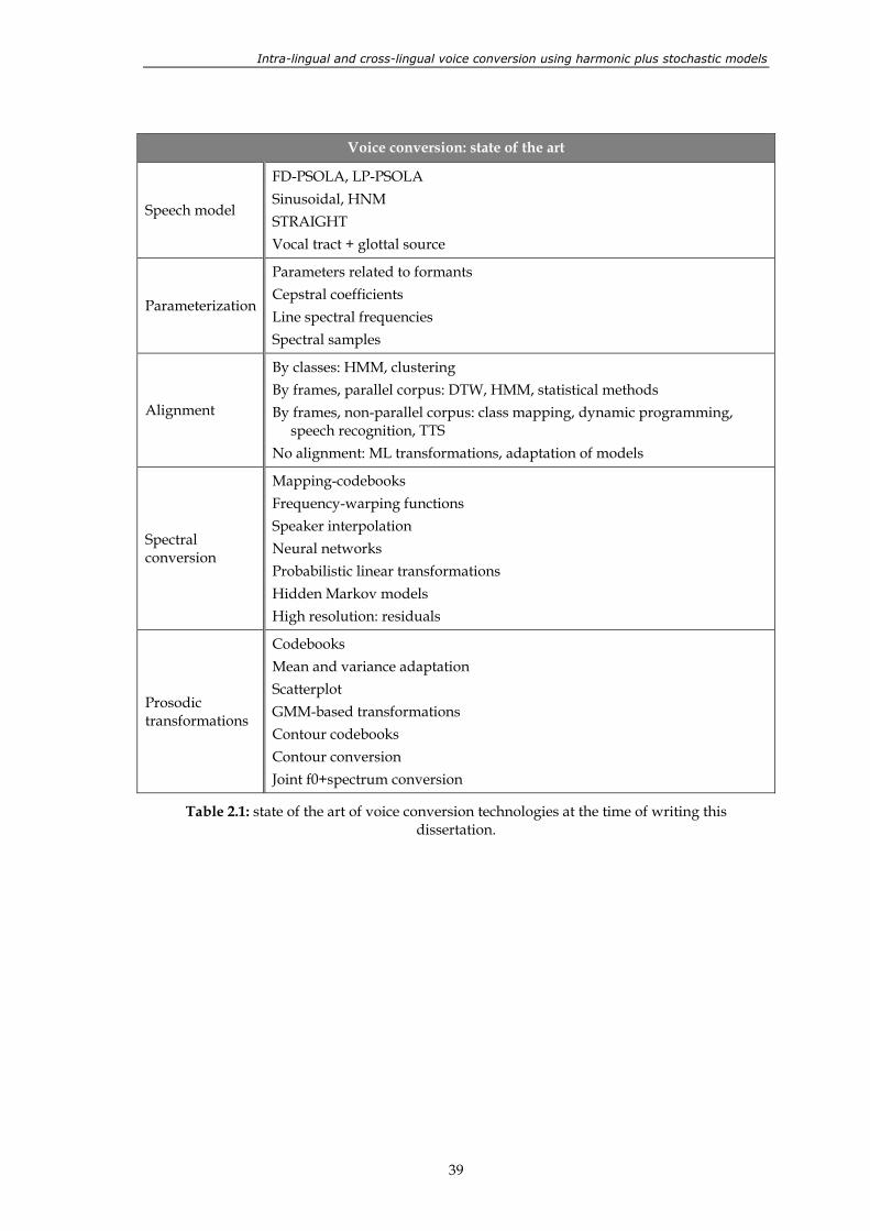
Intra-lingual and cross-lingual voice conversion using harmonic plus stochastic models
39
Voice conversion: state of the art
Speech model
FD-PSOLA, LP-PSOLA Sinusoidal, HNM STRAIGHT Vocal tract + glottal source
Parameterization
Parameters related to formants Cepstral coefficients Line spectral frequencies Spectral samples
Alignment
By classes: HMM, clustering By frames, parallel corpus: DTW, HMM, statistical methods By frames, non-parallel corpus: class mapping, dynamic programming,
speech recognition, TTS No alignment: ML transformations, adaptation of models
Spectral conversion
Mapping-codebooks Frequency-warping functions Speaker interpolation Neural networks Probabilistic linear transformations Hidden Markov models High resolution: residuals
Prosodic transformations
Codebooks Mean and variance adaptation Scatterplot GMM-based transformations Contour codebooks Contour conversion Joint f0+spectrum conversion
Table 2.1: state of the art of voice conversion technologies at the time of writing this dissertation.

Chapter 2. State of the art of voice conversion technologies
40
41
3. Flexible harmonic plus stochastic speech model
The first step before creating a voice conversion system consists of choosing a suitable speech model with certain properties (see figure 3.1). The voice conversion process implies several challenges for which the choice of a suitable speech model is a crucial point: adequate spectral manipulation, adaptation of prosodic contours, etc. As a first condition, the speech model has to be good for synthesis purposes. This condition is satisfied when the model has the following three characteristics:
The analysis-reconstruction of speech signals without modification is transparent or almost-transparent. This means that when a speech signal is analyzed and reconstructed from the model parameters, the resulting signal is perceptually indistinguishable from the original.
The energy, duration and fundamental frequency contours of the speech segments can be modified without introducing audible artifacts into the regenerated signal and without changing the timbre of the original voice, even if the modification factors vary in time.
As the voice conversion technologies are fundamentally addressed to speech synthesis systems based on unit selection and concatenation, the model should provide methods for concatenating speech units selected from different phonetic and prosodic contexts without audible artifacts.
In addition, a fourth condition has to be satisfied for the speech model to be compatible with voice conversion applications:
The model has to allow flexible spectral manipulations.
Finally, there are some other characteristics that are highly desirable for the objectives raised in chapter 1. The voice conversion system to be created has to be compatible with two operation modes: (i) as a stand-alone application that analyzes, converts and synthesizes any input signal; (ii) as a complement for a TTS system that allows customizing the output voice. Particularly for mode (i),
The procedures concerning the analysis, transformation and synthesis processes should be efficient, fully automatic and unsupervised.
This chapter is structured as follows.
In section 3.1, the most common speech models used for synthesis tasks are reviewed and discussed, concluding that the models based on a sinusoidal decomposition are the most suitable according to the objectives of this thesis.
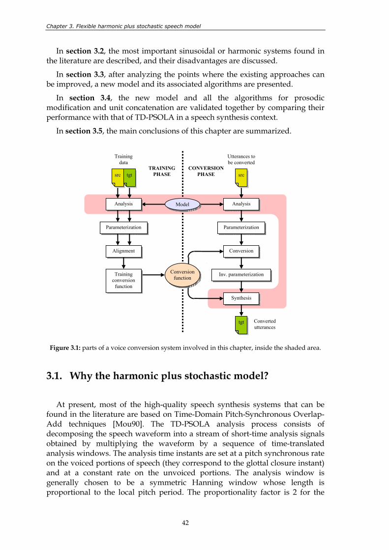
Chapter 3. Flexible harmonic plus stochastic speech model
42
In section 3.2, the most important sinusoidal or harmonic systems found in the literature are described, and their disadvantages are discussed.
In section 3.3, after analyzing the points where the existing approaches can be improved, a new model and its associated algorithms are presented.
In section 3.4, the new model and all the algorithms for prosodic modification and unit concatenation are validated together by comparing their performance with that of TD-PSOLA in a speech synthesis context.
In section 3.5, the main conclusions of this chapter are summarized.
Figure 3.1: parts of a voice conversion system involved in this chapter, inside the shaded area.
3.1. Why the harmonic plus stochastic model?
At present, most of the high-quality speech synthesis systems that can be found in the literature are based on Time-Domain Pitch-Synchronous Overlap-Add techniques [Mou90]. The TD-PSOLA analysis process consists of decomposing the speech waveform into a stream of short-time analysis signals obtained by multiplying the waveform by a sequence of time-translated analysis windows. The analysis time instants are set at a pitch synchronous rate on the voiced portions of speech (they correspond to the glottal closure instant) and at a constant rate on the unvoiced portions. The analysis window is generally chosen to be a symmetric Hanning window whose length is proportional to the local pitch period. The proportionality factor is 2 for the
Converted utterances
Analysis
Parameterization
Alignment
Training conversion
function
Analysis
Parameterization
Conversion
Synthesis
tgt
Inv. parameterization
TRAINING PHASE
CONVERSION PHASE src tgt
Training data
Utterances to be converted
src
Model
Conversion function
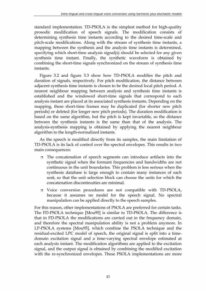
Intra-lingual and cross-lingual voice conversion using harmonic plus stochastic models
43
standard implementation. TD-PSOLA is the simplest method for high-quality prosodic modification of speech signals. The modification consists of determining synthesis time instants according to the desired time-scale and pitch-scale modifications. Along with the stream of synthesis time instants, a mapping between the synthesis and the analysis time instants is determined, specifying which short-time analysis signal(s) should be selected for any given synthesis time instant. Finally, the synthetic waveform is obtained by combining the short-time signals synchronized on the stream of synthesis time instants.
Figure 3.2 and figure 3.3 show how TD-PSOLA modifies the pitch and duration of signals, respectively. For pitch modification, the distance between adjacent synthesis time instants is chosen to be the desired local pitch period. A nearest neighbour mapping between analysis and synthesis time instants is established and the windowed short-time signals that correspond to each analysis instant are placed at its associated synthesis instants. Depending on the mapping, these short-time frames may be duplicated (for shorter new pitch periods) or deleted (for longer new pitch periods). The duration modification is based on the same algorithm, but the pitch is kept invariable, so the distance between the synthesis instants is the same than that of the analysis. The analysis-synthesis mapping is obtained by applying the nearest neighbour algorithm to the length-normalized instants.
As the speech is modified directly from its samples, the main limitation of TD-PSOLA is its lack of control over the spectral envelopes. This results in two main consequences:
The concatenation of speech segments can introduce artifacts into the synthetic signal when the formant frequencies and bandwidths are not continuous in the unit boundaries. This problem is less serious when the synthesis database is large enough to contain many instances of each unit, so that the unit selection block can choose the units for which the concatenation discontinuities are minimal.
Voice conversion procedures are not compatible with TD-PSOLA, because it assumes no model for the speech signal. No spectral manipulation can be applied directly to the speech samples.
For this reason, other implementations of PSOLA are preferred for certain tasks. The FD-PSOLA technique [Mou95] is similar to TD-PSOLA. The difference is that in FD-PSOLA the modifications are carried out in the frequency domain, and therefore the spectral manipulation ability is not a problem anymore. In LP-PSOLA systems [Mou95], which combine the PSOLA technique and the residual-excited LPC model of speech, the original signal is split into a time-domain excitation signal and a time-varying spectral envelope estimated at each analysis instant. The modification algorithms are applied to the excitation signal, and the output signal is obtained by combining the modified excitation with the re-synchronized envelopes. These PSOLA implementations are more
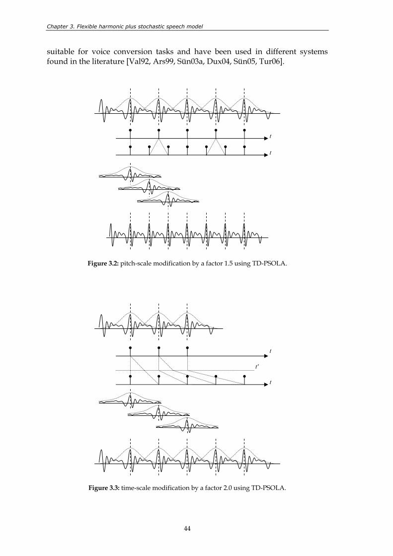
Chapter 3. Flexible harmonic plus stochastic speech model
44
suitable for voice conversion tasks and have been used in different systems found in the literature [Val92, Ars99, Sün03a, Dux04, Sün05, Tur06].
Figure 3.2: pitch-scale modification by a factor 1.5 using TD-PSOLA.
Figure 3.3: time-scale modification by a factor 2.0 using TD-PSOLA.
t
t
t'
t
t
Intra-lingual and cross-lingual voice conversion using harmonic plus stochastic models
45
The speech signal representation using STRAIGHT [Kaw97] is also useful for conversion purposes. STRAIGHT performs a pitch-adaptive spectral analysis in order to obtain a time-frequency surface that represents the time-varying magnitude envelope. For the speech reconstruction, an excitation signal based on phase manipulation is built and combined with the parameterized envelope. This model allows very high manipulation factors for pitch and duration without further degradation. On the other hand, this kind of representation involves information expansion rather than reduction. Thus, its main applications are related to voice conversion and speech manipulation, since the spectral envelopes are well characterized and certain parameters like complex cepstrum, which is very useful in many areas of speech technologies, are easily obtained from them. On the contrary, it is not suitable for high quality synthesis because it would have strong memory requirements due to the information expansion, whereas the quality of the synthetic speech is worse than that obtained by PSOLA systems. STRAIGHT representation has been used in several voice conversion systems [Tod01, Tod05, Tod06].
The so called sinusoidal models assume that the speech waveform can be locally represented by a sum of sinusoids with time-varying parameters. Harmonic models are a special case of sinusoidal models in which the frequencies of the sinusoids are restricted to be integer multiples of the local fundamental frequency. There are several reasons why sinusoidal models are very appropriate for all kind of voice transformations:
They provide a framework for high quality speech reconstruction and prosodic modification.
The parameters of the sinusoids carry important information from the waveform but also from the spectrum. Good estimates for magnitude and phase spectral envelopes can be extracted from the model parameters, and therefore the model provides maximal flexibility for spectral manipulation and voice conversion.
As a consequence of this, the model has good physical properties for concatenative speech synthesis, because it allows suppressing the waveform and spectral discontinuities at the boundaries between two adjacent units.
In addition, it allows data compression for embedded systems.
Finally, it is compatible with all the voice conversion methods reviewed in chapter 2. Thus, many of the most relevant voice conversion systems are based on such models [Sty98, Kai01, Ye06, Shu06, Err07a].
Hybrid models are based on a deterministic plus stochastic decomposition of speech: the deterministic part is sinusoidal (or harmonic), and the stochastic part deals with all the signal aperiodic components that are not well represented by sinusoids. The main advantage of hybrid models, apart from those of pure sinusoidal models, is that both signal components, which are
Chapter 3. Flexible harmonic plus stochastic speech model
46
different in nature, can be treated in a different way. This is useful for high-quality speech synthesis, because it helps to avoid the tonal artifacts that appear when PSOLA-like techniques are applied to modify unvoiced sounds [Sty96]. In voice conversion systems a two-component model is also useful, since transforming the voiced segments of speech is much more important for the similarity between converted and target voices than transforming the unvoiced segments (where the deterministic component is zero) [Ye04a]. In addition, controlling the energy carried by both components in voiced segments allows manipulating the voice quality to a certain extent. On the other hand, splitting the signal into two different components and designing appropriate transformation functions for both is not straightforward. However, in this thesis a harmonic plus stochastic model (HSM) has been used for analyzing, modifying, manipulating and synthesizing the speech signals.
As a final remark, in contrast to all the models reviewed above, in which the speech signal is manipulated considering how the transformed signal is perceived by listeners, source-filter models trying to capture the mechanisms of speech production have been recently applied to voice transformation tasks [Vin07]. Although voice conversion results are not visible yet, the characteristics of such models seem to be very appropriate for voice conversion applications, because theoretically, parameterizing both the glottal source and the vocal tract allows better capturing the differences between speakers and easily manipulating speech properties like voice quality. Thus, it is expected that significant progress will be made during the next years by means of this kind of models.
3.2. Sinusoidal and hybrid systems: a bibliographic study
A wide variety of consolidated systems based on a sinusoidal or harmonic decomposition can be found in the literature. Although most of them are not hybrid systems, the associated algorithms related to manipulation of signals decomposed into sinusoids are valid also for the deterministic component of hybrid systems. In general, many solutions have been proposed for the following two problems:
Accurate analysis and reconstruction of speech signals. In general, natural speech signals and signals reconstructed from this kind of parameters are indistinguishable, so the most important problem is the second one.
High-quality prosodic modification of speech without breaking the inter-frame phase coherence and the waveform shape invariance. Preserving the phase coherence means avoiding the appearance of waveform discontinuities, which are usually related to the phases of the sinusoids.
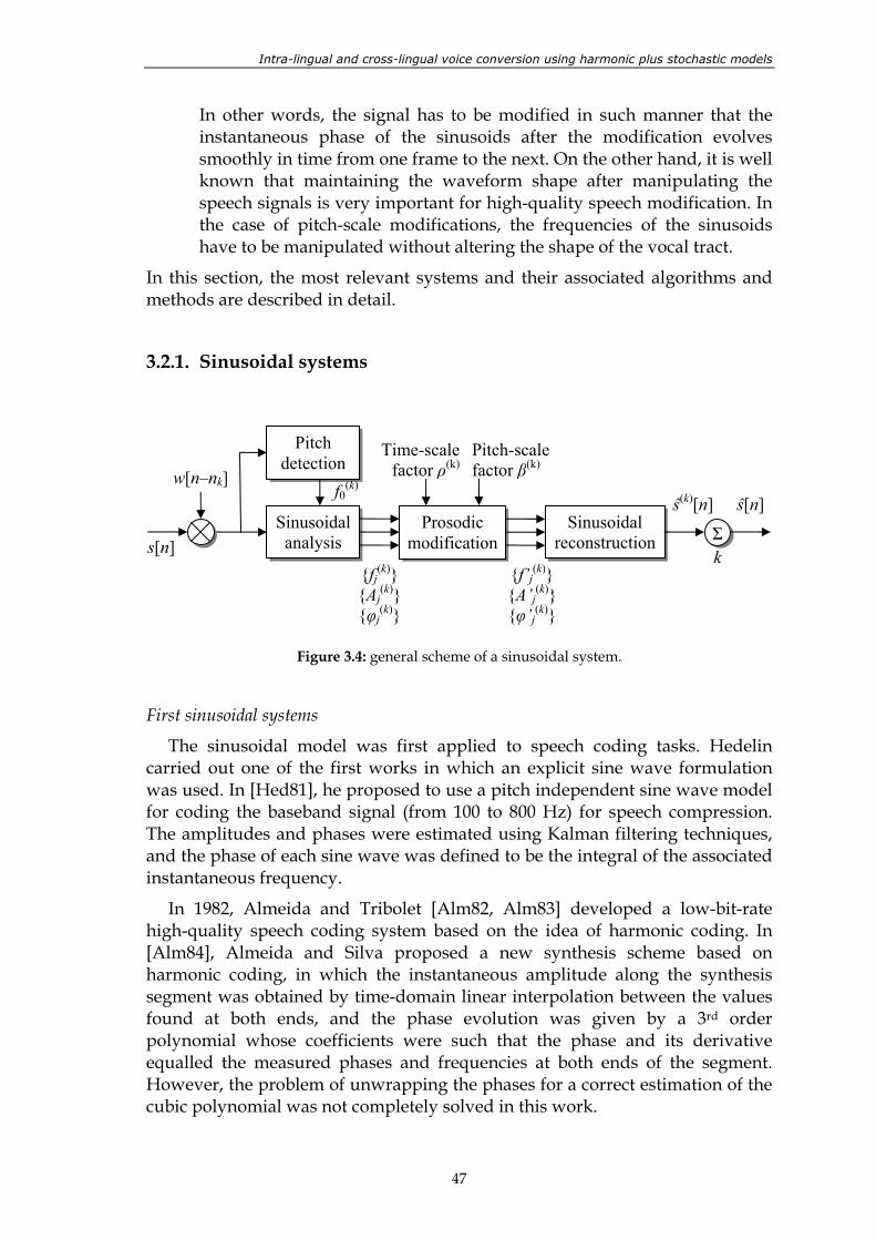
Intra-lingual and cross-lingual voice conversion using harmonic plus stochastic models
47
In other words, the signal has to be modified in such manner that the instantaneous phase of the sinusoids after the modification evolves smoothly in time from one frame to the next. On the other hand, it is well known that maintaining the waveform shape after manipulating the speech signals is very important for high-quality speech modification. In the case of pitch-scale modifications, the frequencies of the sinusoids have to be manipulated without altering the shape of the vocal tract.
In this section, the most relevant systems and their associated algorithms and methods are described in detail.
3.2.1. Sinusoidal systems
Figure 3.4: general scheme of a sinusoidal system.
First sinusoidal systems
The sinusoidal model was first applied to speech coding tasks. Hedelin carried out one of the first works in which an explicit sine wave formulation was used. In [Hed81], he proposed to use a pitch independent sine wave model for coding the baseband signal (from 100 to 800 Hz) for speech compression. The amplitudes and phases were estimated using Kalman filtering techniques, and the phase of each sine wave was defined to be the integral of the associated instantaneous frequency.
In 1982, Almeida and Tribolet [Alm82, Alm83] developed a low-bit-rate high-quality speech coding system based on the idea of harmonic coding. In [Alm84], Almeida and Silva proposed a new synthesis scheme based on harmonic coding, in which the instantaneous amplitude along the synthesis segment was obtained by time-domain linear interpolation between the values found at both ends, and the phase evolution was given by a 3rd order polynomial whose coefficients were such that the phase and its derivative equalled the measured phases and frequencies at both ends of the segment. However, the problem of unwrapping the phases for a correct estimation of the cubic polynomial was not completely solved in this work.
Sinusoidal analysis
w[n–nk]
s[n]
Pitch detection
f0(k)
fj(k)
Aj(k)
φj(k)
Time-scale factor ρ(k)
Prosodic modification
f’j(k)
A’j(k)
φ’j(k)
Pitch-scale factor β(k)
Sinusoidal reconstruction Σ
ŝ(k)[n] ŝ[n]
k
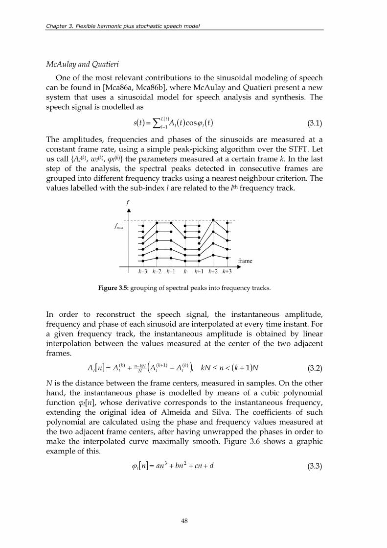
Chapter 3. Flexible harmonic plus stochastic speech model
48
McAulay and Quatieri
One of the most relevant contributions to the sinusoidal modeling of speech can be found in [Mca86a, Mca86b], where McAulay and Quatieri present a new system that uses a sinusoidal model for speech analysis and synthesis. The speech signal is modelled as
( ) ( ) ( )( )∑ ==
tL
l ll ttAts1
cosϕ (3.1)
The amplitudes, frequencies and phases of the sinusoids are measured at a constant frame rate, using a simple peak-picking algorithm over the STFT. Let us call Al(k), wl(k), φl(k) the parameters measured at a certain frame k. In the last step of the analysis, the spectral peaks detected in consecutive frames are grouped into different frequency tracks using a nearest neighbour criterion. The values labelled with the sub-index l are related to the lth frequency track.
Figure 3.5: grouping of spectral peaks into frequency tracks.
In order to reconstruct the speech signal, the instantaneous amplitude, frequency and phase of each sinusoid are interpolated at every time instant. For a given frequency track, the instantaneous amplitude is obtained by linear interpolation between the values measured at the center of the two adjacent frames.
[ ] ( ) ( )NknkNAAAnA kl
klN
kNnkll 1,)()1()( +<≤−+= +− (3.2)
N is the distance between the frame centers, measured in samples. On the other hand, the instantaneous phase is modelled by means of a cubic polynomial function φl[n], whose derivative corresponds to the instantaneous frequency, extending the original idea of Almeida and Silva. The coefficients of such polynomial are calculated using the phase and frequency values measured at the two adjacent frame centers, after having unwrapped the phases in order to make the interpolated curve maximally smooth. Figure 3.6 shows a graphic example of this.
[ ] dcnbnannl +++= 23ϕ (3.3)
f
frame
k k+1 k+2 k+3k–1k–2k–3
fmax
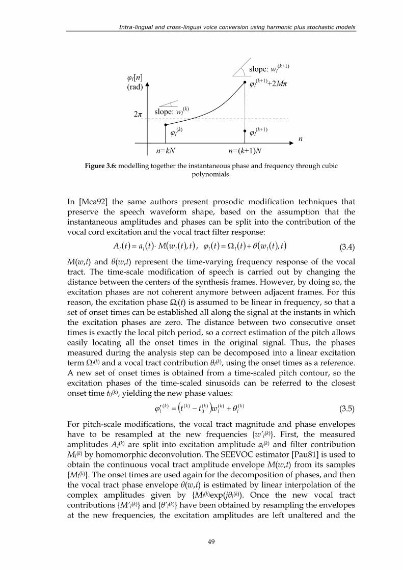
Intra-lingual and cross-lingual voice conversion using harmonic plus stochastic models
49
Figure 3.6: modelling together the instantaneous phase and frequency through cubic
polynomials.
In [Mca92] the same authors present prosodic modification techniques that preserve the speech waveform shape, based on the assumption that the instantaneous amplitudes and phases can be split into the contribution of the vocal cord excitation and the vocal tract filter response:
( ) ( ) ( )( ) ( ) ( ) ( )( )ttwttttwMtatA llllll , , , θϕ +Ω=⋅= (3.4)
M(w,t) and θ(w,t) represent the time-varying frequency response of the vocal tract. The time-scale modification of speech is carried out by changing the distance between the centers of the synthesis frames. However, by doing so, the excitation phases are not coherent anymore between adjacent frames. For this reason, the excitation phase Ωl(t) is assumed to be linear in frequency, so that a set of onset times can be established all along the signal at the instants in which the excitation phases are zero. The distance between two consecutive onset times is exactly the local pitch period, so a correct estimation of the pitch allows easily locating all the onset times in the original signal. Thus, the phases measured during the analysis step can be decomposed into a linear excitation term Ωl(k) and a vocal tract contribution θl(k), using the onset times as a reference. A new set of onset times is obtained from a time-scaled pitch contour, so the excitation phases of the time-scaled sinusoids can be referred to the closest onset time t0(k), yielding the new phase values:
( ) )()()(0
)()( kl
kl
kkkl wtt θϕ +−=′ (3.5)
For pitch-scale modifications, the vocal tract magnitude and phase envelopes have to be resampled at the new frequencies w’l(k). First, the measured amplitudes Al(k) are split into excitation amplitude al(k) and filter contribution Ml(k) by homomorphic deconvolution. The SEEVOC estimator [Pau81] is used to obtain the continuous vocal tract amplitude envelope M(w,t) from its samples Ml(k). The onset times are used again for the decomposition of phases, and then the vocal tract phase envelope θ(w,t) is estimated by linear interpolation of the complex amplitudes given by Ml(k)exp(jθl(k)). Once the new vocal tract contributions M’l(k) and θ’l(k) have been obtained by resampling the envelopes at the new frequencies, the excitation amplitudes are left unaltered and the
n φl
(k+1) φl(k)
φl(k+1)+2Mπ
2π
n=(k+1)N n=kN
slope: wl(k)
slope: wl(k+1)
φl[n] (rad)
Chapter 3. Flexible harmonic plus stochastic speech model
50
excitation phases are readjusted using the set of onset times associated to the transformed pitch contour. Both the time-scale and pitch-scale modification factors can vary in time.
Analysis-by-Synthesis/Overlap-Add
The Analysis-by-Synthesis/Overlap-Add (ABS/OLA) sinusoidal model proposed by George and Smith [Geo87, Geo92, Geo97] has some remarkable peculiarities with respect to others. The first one is that the amplitudes, frequencies and phases of the sinusoids are determined at a constant frame rate using an ABS procedure: assuming that l-1 sinusoids have been detected and subtracted from the original kth signal frame, the next sinusoid l is detected from the remaining residual by calculating the parameters Al(k), wl(k), φl(k) that minimize the energy of the estimation error. For a given candidate frequency wl(k), the optimal amplitude and phase can be calculated by least-squares optimization, so the best combination of parameters is chosen by evaluating the error at uniformly spaced candidate frequencies. The second particularity of the model is that the time-varying waveform is reconstructed by overlapping frames that contain sums of constant-amplitude constant-frequency sinusoids
[ ] [ ] [ ] [ ] [ ] ( )∑∑=
+=−−=)(
1
)()()()()( cos ,kL
l
kl
kl
kl
k
k
k nwAnskNnskNnwnns ϕσ (3.6)
where w[n] is the window used for OLA, σ[n] is a time-varying gain function and N is the number of samples that correspond to the analysis frame rate. In order to facilitate the prosodic modification of speech, a quasi-harmonic version of the previous model is used: the measured frequency wl(k) is split into a harmonic term, lw0(k), and a deviation term, ∆l(k). The time-scale modified speech is obtained by modifying the distance between frame centers, N. A graphic description is shown in figure 3.7. The samples of the time-scaled frames are given by the following expression, in which ρ(k) is the modification factor at frame k (ρ>1 means lengthening the signal and ρ<1 means shortening it):
[ ] ( )( )∑=
+∆++=)(
)(
1
)()(1)()(0
)()( cosk
k
L
l
kl
kl
kkkl
k nnlwAns ϕδρ
(3.7)
The deviation from the ideal harmonic frequency ∆l(k) is divided by ρ(k) in order to avoid the excessive shape invariance when the frame length is increased. The parameter δ(k) expresses a linear phase correction that is necessary to ensure the inter-frame phase coherence despite the modification. For the pitch modification, the vocal tract filter H(k) is estimated at each frame and the vocal tract amplitude and phase contributions are removed from the signal, so that the excitation signal is isolated and represented by the residual amplitudes, al(k), and phases, Ωl(k). A continuous excitation spectrum is estimated by interpolating the complex phasor form of the excitation amplitude-phase pairs. Given a pitch-scale factor β(k), the excitation spectrum is then resampled at modified harmonic frequencies to generate new phasor values from which the target amplitudes a’l(k) and phases Ω’l(k) are extracted. The frequency deviation
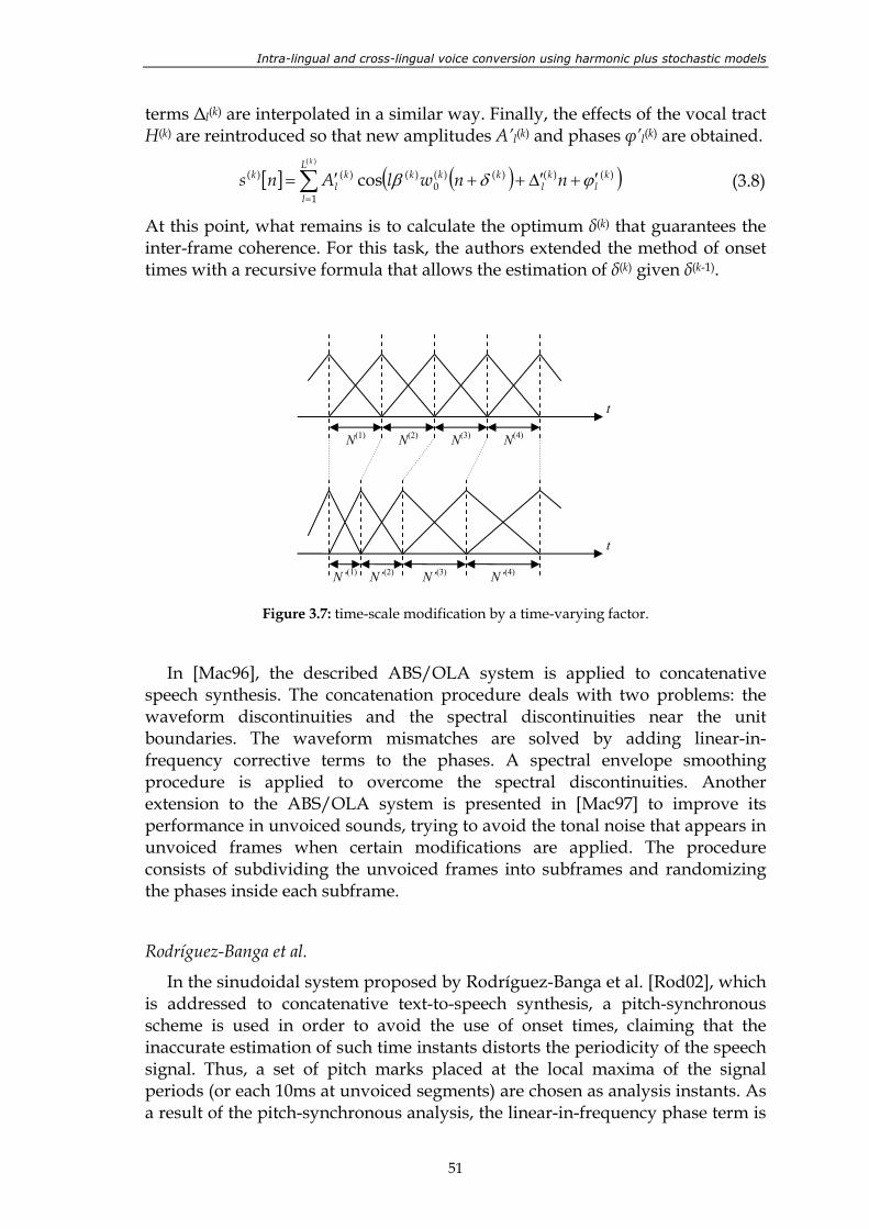
Intra-lingual and cross-lingual voice conversion using harmonic plus stochastic models
51
terms ∆l(k) are interpolated in a similar way. Finally, the effects of the vocal tract H(k) are reintroduced so that new amplitudes A’l(k) and phases φ’l(k) are obtained.
[ ] ( )( )∑=
′+∆′++′=)(
1
)()()()(0
)()()( coskL
l
kl
kl
kkkkl
k nnwlAns ϕδβ (3.8)
At this point, what remains is to calculate the optimum δ(k) that guarantees the inter-frame coherence. For this task, the authors extended the method of onset times with a recursive formula that allows the estimation of δ(k) given δ(k-1).
Figure 3.7: time-scale modification by a time-varying factor.
In [Mac96], the described ABS/OLA system is applied to concatenative speech synthesis. The concatenation procedure deals with two problems: the waveform discontinuities and the spectral discontinuities near the unit boundaries. The waveform mismatches are solved by adding linear-in-frequency corrective terms to the phases. A spectral envelope smoothing procedure is applied to overcome the spectral discontinuities. Another extension to the ABS/OLA system is presented in [Mac97] to improve its performance in unvoiced sounds, trying to avoid the tonal noise that appears in unvoiced frames when certain modifications are applied. The procedure consists of subdividing the unvoiced frames into subframes and randomizing the phases inside each subframe.
Rodríguez-Banga et al.
In the sinudoidal system proposed by Rodríguez-Banga et al. [Rod02], which is addressed to concatenative text-to-speech synthesis, a pitch-synchronous scheme is used in order to avoid the use of onset times, claiming that the inaccurate estimation of such time instants distorts the periodicity of the speech signal. Thus, a set of pitch marks placed at the local maxima of the signal periods (or each 10ms at unvoiced segments) are chosen as analysis instants. As a result of the pitch-synchronous analysis, the linear-in-frequency phase term is
N(1) N(2) N(3) N(4)
N’(1) N’(2) N’(3) N’(4)
t
t
Chapter 3. Flexible harmonic plus stochastic speech model
52
assumed to be zero at every frame, so when pitch-scale modifications are applied, the vocal tract phase envelope can be estimated directly by linear interpolation of the measured complex amplitudes. The amplitude envelope is obtained by linear interpolation of the measured log-amplitudes. A new set of pitch marks derived from the desired f0-contour are used as onset times for synthesis.
O’Brien and Monaghan
The harmonic analysis/synthesis system presented by O’Brien and Monaghan [Obr01] provides modification procedures that do not require the usage of pitch marks, onset times or pitch-synchronous schemes. Instead, the inter-frame coherence and shape invariance are ensured by an adequate manipulation of 3rd order polynomials representing the instantaneous phase. McAulay and Quatieri stated that the instantaneous phase of a given sinusoids can be modelled in an N-length interval by a cubic polynomial whose coefficients are calculated according to the phases and frequencies detected in both ends of the interval. According to the same formulation of expression (3.3), the instantaneous frequency is given by
[ ] cbnannl ++= 23 2ϕ& (3.9)
For time-scaling the kth frame by a factor ρ(k), the instantaneous frequency is time-scaled to lie into the interval [0, Nρ(k)]. The new phase trajectory corresponds to the integral of the modified frequency trajectory, so the new phase values at k+1 can be calculated from those of k by the following recursion:
[ ] ( )cbNaNNdnn kkl
N kl
kl
kl
k
+++′=+′=′ ∫+ 2)()(
0
)()()1()(
ρϕρϕϕϕρ
& (3.10)
In order to keep the waveform shape invariant, the first harmonic is used to establish a single linear-in-frequency phase correction term for frame k+1:
)1()1()1()1(1
)1(1
)1( , ++++++ +=′−′= kkl
kl
kkk lδϕϕϕϕδ (3.11)
The time-scaled speech signal is then synthesized directly from the modified parameters. A similar idea is followed for the pitch-scale modification of speech, but previously the Iterative Adaptive Inverse Filtering technique (IAIF) [Alk91] is applied to the original signal in order to isolate the LPC excitation component, which is then analyzed and parameterized according to the harmonic model. Assuming that the modification factor β is different for each frame, the frequency trajectory can be multiplied by a linearly-varying factor.
[ ] ( )( )( ) ( ) ( )[ ])1()()1()()1()(2
121)(
0
)()1()()()1(
62433 +++
++
++++++′=
=−+⋅+′=′ ∫kkkkkkk
l
N kkNnk
lk
lk
l
cbNaNN
dnn
ββββββϕ
βββϕϕϕ & (3.12)
Again, the linear-in-frequency phase correction term δ(k+1) is calculated for the first harmonic and is then generalized to the rest. Finally, the new vocal tract contribution is added to the amplitudes and phases. The authors propose also a similar solution for the problem of concatenating units with phase mismatches,
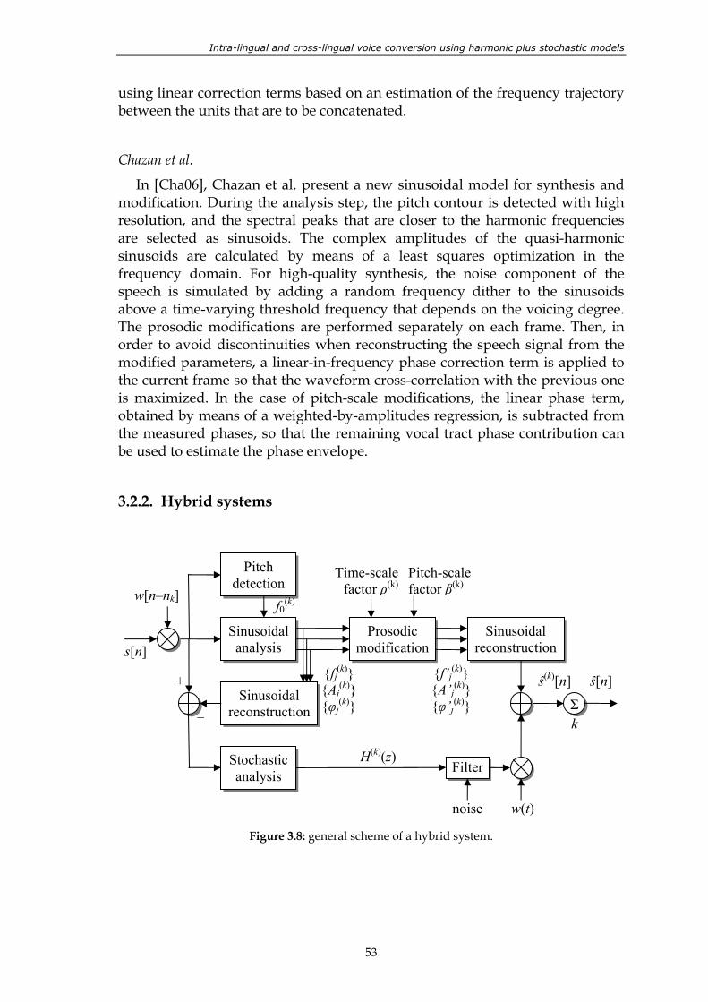
Intra-lingual and cross-lingual voice conversion using harmonic plus stochastic models
53
using linear correction terms based on an estimation of the frequency trajectory between the units that are to be concatenated.
Chazan et al.
In [Cha06], Chazan et al. present a new sinusoidal model for synthesis and modification. During the analysis step, the pitch contour is detected with high resolution, and the spectral peaks that are closer to the harmonic frequencies are selected as sinusoids. The complex amplitudes of the quasi-harmonic sinusoids are calculated by means of a least squares optimization in the frequency domain. For high-quality synthesis, the noise component of the speech is simulated by adding a random frequency dither to the sinusoids above a time-varying threshold frequency that depends on the voicing degree. The prosodic modifications are performed separately on each frame. Then, in order to avoid discontinuities when reconstructing the speech signal from the modified parameters, a linear-in-frequency phase correction term is applied to the current frame so that the waveform cross-correlation with the previous one is maximized. In the case of pitch-scale modifications, the linear phase term, obtained by means of a weighted-by-amplitudes regression, is subtracted from the measured phases, so that the remaining vocal tract phase contribution can be used to estimate the phase envelope.
3.2.2. Hybrid systems
Figure 3.8: general scheme of a hybrid system.
Sinusoidal analysis
w[n–nk]
s[n]
Pitch detection
f0(k)
fj(k)
Aj(k)
φj(k)
Time-scale factor ρ(k)
Prosodic modification
f’j(k)
A’j(k)
φ’j(k)
Pitch-scale factor β(k)
Sinusoidal reconstruction
Σ
ŝ(k)[n] ŝ[n]
k
Sinusoidal reconstruction
+
–
Stochastic analysis
H(k)(z)
w(t)
Filter
noise
Chapter 3. Flexible harmonic plus stochastic speech model
54
First hybrid systems
In [Gri88], Griffin and Lim proposed a new system called Multiband Excitation Vocoder. In this model, the short-time spectrum of speech is modelled as the product of an excitation spectrum and a spectral envelope. The spectral envelope is a smoothed version of the speech spectrum, and the excitation spectrum is represented by a fundamental frequency, a voiced/unvoiced decision for each harmonic, and the phase of each harmonic declared voiced. This is one of the first studies in which the speech is treated as the sum of a harmonic component and a noise-like component. The model proposed by Abrantes et al. [Abr91] also represents the speech signal as a sum of harmonically related sinusoids and band-pass random signals. However, these models were used only in speech coding applications.
Serra
In other works like those carried out by Serra [Ser89, Ser97], a deterministic plus stochastic model is used for analysis, modification and synthesis of musical sounds. In essence, the model is similar to that defined by McAulay and Quatieri, but a noise-like component is introduced to deal with excitation mechanisms and energy components that are not sinusoidal in nature. Thus, during the analysis, the sinusoidal component is regenerated from the measured parameters and is subtracted from the original waveform in order to isolate the stochastic component. As this residual component is well characterized by its power spectral density instead of its waveform, linear predictive coding (LPC) techniques are used for analyzing and synthesizing it. It is highly remarkable that in Serra’s system the phase information is not used for synthesis, so it can be discarded after the analysis process. The instantaneous phase of each sinusoid is interpolated assuming that the frequency evolves linearly from one frame to the next. As the synthesis phase values are calculated recursively, the first value of each frequency track is initialized with a random number.
[ ] ( )[ ] [ ]( ) ( )NknkN
NwkNnnwn
wwwnw
kl
kl
kl
lk
ll
kl
klN
kNnkll
1
ˆˆˆ
)1()()1(
)(
)()1()(
+<≤
+=
−+=
−+=
++
+−
ϕϕ
ϕθ (3.13)
Although this synthesis scheme was successfully applied to musical signals, it was also proved that the magnitude-only reconstructed speech has an unnatural tonal quality [Mca84, Mca86b]. In the speech coding field, some approaches were also proposed to avoid the need of preserving the measured phases: approximating the real phase envelope by the minimum-phase response of an all-pole filter, improving the minimum-phase response by means of corrective all-pass filters, etc. [Mar90, Mca95, Ahm98]. Although these techniques have some advantages for speech coding, they do not provide high-quality synthetic speech.
Intra-lingual and cross-lingual voice conversion using harmonic plus stochastic models
55
Harmonic plus Noise Model
The Harmonic plus Noise Model (HNM) has become one of the most popular models for speech synthesis and modification [Lar93, Sty95, Sty96]. The model is based on the decomposition of the speech signal s(t) into a deterministic part d(t) and a stochastic part e(t). The deterministic component is a sum of harmonically related sinusoidal components with piecewise linearly varying complex amplitudes. It can be defined at specific time instants ti as
( ) ( ) ( ) ( )( )( )
221
0expRe Ti
Ti
tL
liiil ttttttjlwtCtd ∆∆
=
+<≤−
−⋅⋅= ∑ (3.14)
where Cl are the complex amplitudes of the harmonics, ∆T is the frame length and L(t) represents the number of harmonics, which is defined according to a time-varying maximum voicing frequency. The stochastic part is obtained by filtering a white gaussian noise n(t) by a time-varying all-pole filter H(t, z) and multiplying the result by an energy-envelope function w(t).
( ) ( ) ( ) ( )[ ]tnztHtwte ∗⋅= , (3.15)
During the analysis, once the w0-contour is estimated, the analysis time instants ti are set at a pitch synchronous rate on the voiced portions of speech, and at a fixed rate of 10ms on unvoiced segments. The harmonic parameters are estimated below the maximum voicing frequency by means of a weighted least-squares method in the time domain. The deterministic part is then subtracted from the original signal and the residual’s spectral density function is modelled by fitting an all-pole filter H(ti,z). Finally, the temporal energy distribution of the stochastic component is modelled by a parametric triangular-like time-domain envelope w(t). The reconstruction of the signal from the measured parameters is carried out as follows. The synthesis time instants, ti’, correspond exactly to those used for the analysis. The harmonic component is interpolated in the time domain, whereas the stochastic component is the result of passing white gaussian noise through H(t,z), high-pass filtering according to the instantaneous maximum voicing frequency, and finally applying the time-domain envelope w(t) on voiced segments.
The prosodic modification procedures of HNM are based on the PSOLA technique. A set of synthesis time-instants is derived from the modified pitch contour, and a mapping is established between analysis and synthesis time instants. The time-scale modification is performed by deleting/duplicating frames and the pitch-scale modification consists of altering the distance between the analysis instants and resampling the amplitude and phase envelopes at the new harmonic frequencies. No correction is needed for the phases, since the frame rate is pitch-synchronous. The amplitude envelope is defined using discrete cepstral coefficients that are estimated by means of a frequency-domain least-squares criterion, whereas the phase envelope is built by linear interpolation of the unwrapped phases.
Two conceptually different versions of HNM, called HSM (harmonic plus stochastic model) and DSM (deterministic plus stochastic model), can be found
Chapter 3. Flexible harmonic plus stochastic speech model
56
in [sty96], but although they entail more complicated analysis procedures, they do not lead to significant improvements in terms of perceptual quality. HNM was applied to speech synthesis [Sty01a] and voice conversion [Sty98] with very good results. Furthermore, in [Syr98] HNM was compared to TD-PSOLA from different points of view, concluding that HNM gives better overall performance because it allows smoothing the unit boundaries in concatenative synthesis, it yields more natural-sounding synthetic speech and it has better properties for compression and for voice conversion.
Stochastic component manipulation
Regarding the aperiodic part of voiced speech, it was stated by Hermes [Her91] that the time-domain characteristics of the stochastic component are also important for the overall perceptual quality. For this reason, Stylianou’s HNM uses a pitch-synchronous triangular-like envelope to modulate the energy of the stochastic component inside each period, so that the maximum-energy instants of the deterministic and stochastic components are synchronized [Sty96]. This condition is important when the stochastic component is modelled by means of high-pass noise, since listeners seem to perceive two independent audio sources when no time-modulation is performed. Theoretically, this approach is no longer valid when the stochastic component occupies the full analysis band (there is no reason to suppose that the harmonic bands do not contain aperiodic information [Sty96, Yeg98]), so in this case the synchronization problem requires using different specific techniques like formant waveforms [Ric96], applied after an accurate deterministic-plus-stochastic decomposition [Yeg98, Ahn97]. However, in practice, the stochastic model based on time-modulated filtered noise gives also satisfactory results in this situation: in [Bai01], a period-normalized parametric envelope is fitted to the stochastic component during analysis, and during the synthesis procedure the filtered noise frames are multiplied by the period-adapted envelope.
3.2.3. Discussion
According to the objectives of the thesis, the implemented system has to be suitable for generating converted synthetic speech, but also for converting natural speech signals. Some of the approaches described above are pitch-synchronous, like Stylianou’s HNM or the system proposed by Banga et al. The motivation for using a pitch synchronous scheme is to facilitate the reconstruction of the signal from its periods without problems derived from the phase. In exchange, the signal periods have to be correctly separated during the analysis step, so an accurate control over the analysis instants is necessary. This limitation is not important in the case of TTS systems, where the synthesis databases are created off-line and thus the analysis can be validated, but in the case of real-time voice conversion systems, for instance, a pitch-synchronous
Intra-lingual and cross-lingual voice conversion using harmonic plus stochastic models
57
analysis may cause problems. On the contrary, a constant frame rate analysis simplifies the analysis process and makes the system compatible with such applications. Even if the system requires estimating the pitch at each frame, it is easier to estimate the pitch than to calculate exact pitch epochs appearing at a pitch-synchronous rate. In addition, this type of analysis allows the user to have a certain control over the number of analysis frames extracted from a given utterance, so the computational load and memory requirements can also be controlled, whereas in pitch-synchronous schemes the frame rate and the time resolution of the analysis is fixed by the local period length. The main drawback of analysis schemes that are not pitch-synchronous is that the inter-frame coherence and the intra-frame shape invariance are more difficult to preserve from degradation. For this reason, several pitch-asynchronous systems, like the one proposed by McAulay and Quatieri or the ABS/OLA system designed by George and Smith, follow an intermediate approach based on handling a set of onset times whose separation is the measured local pitch period, but the inaccurate estimation of such instants causes audible artifacts. From this point of view, O’Brien and Monaghan’s system is very interesting because it combines pitch-asynchronous analysis and phase modification without onset times. Unfortunately, it has other disadvantages like requiring inverse filtering techniques. The sinusoidal system of Chazan et al. uses phase correction based on cross-correlation maximization to make the adjacent frames (modified or not) coherent, but in the next section it is proved that a satisfactory performance is obtained by means of a much simpler approach.
Concerning the pitch modification algorithms, which are closely related to the estimation of amplitude and phase envelopes, important differences can be observed between the described systems. Some of them need an explicit decomposition into excitation signal and vocal tract contribution: McAulay-Quatieri, ABS-OLA, and O’Brien-Monaghan. In the rest of the systems the amplitude and phase envelopes are treated as if they corresponded exactly to the vocal tract contribution, which is equivalent to supposing that the spectrum of the excitation signal has constant amplitude and linear-in-frequency phases. The performance of such systems is not affected by the simplification of the speech production model, so the procedures for vocal tract estimation and inverse filtering can be replaced by simple envelope estimation procedures with lower associated computational cost, without worrying about the quality. Extracting the amplitude envelope from the measured amplitudes is not problematic at all: linear interpolation is accurate enough. Extracting the phase envelopes from the measured phases is straightforward only in the case of pitch-synchronous systems like HNM, whereas in non-pitch-synchronous systems, as it has been mentioned above, it is more complicated to deal with phases without using onset times. Therefore, adopting a pitch-asynchronous scheme in order to simplify the requirements of the analysis step implies making the modification procedures more complicated, unless a simple procedure for cancelling the linear phase term is also provided. Chazan’s pitch-
Chapter 3. Flexible harmonic plus stochastic speech model
58
asynchronous system incorporates a solution for this problem. In the next section, another new solution is proposed.
Concerning the aperiodic components of speech, in pure sinusoidal systems the unvoiced bands are also modelled by means of sinusoidal parameters, but special techniques for phase manipulation or frequency dithering are necessary to preserve the noisy perceptual aspect of such components. Moreover, using a sinusoidal representation, the aperiodic component has to be restricted to the non-voiced bands. In hybrid systems like HNM, the aperiodic component of speech is described by a separate stochastic model, which is advantageous because it allows modelling wideband noisy components by means of few parameters. Although in a typical HNM implementation the voiced and unvoiced bands are separated by a time-varying cut-off frequency, there is no physical reason to suppose that they are non-overlapping components. It also has to be taken into account that in a voice conversion system it is desirable to use a constant maximum voicing frequency, so that the spectral envelopes (obtained from the parameters of the detected sinusoids) are defined within the same frequency range for all the frames and for every speaker. Nevertheless, modeling the time-domain characteristics of the wideband stochastic component is problematic, because the synchronization properties of time-domain envelopes may disappear when voices are converted into other voices, unless the envelopes are also converted. Therefore, it seems advisable to look for an easier way of synchronizing the signal components if a hybrid model of speech with wideband stochastic component is adopted.
3.3. Proposed algorithms for a pitch-asynchronous scheme
This section presents a speech model designed during this thesis to fit the specifications analyzed above. It has the following characteristics:
It is based on a harmonic plus stochastic decomposition.
In voiced frames, a fixed maximum voicing frequency is used to delimitate the harmonic band. A wideband stochastic component is used.
The system and algorithms are compatible with a non-pitch-synchronous frame rate analysis scheme. For this purpose, new procedures for time-scale and pitch-scale modification of speech are provided. These procedures are conceptually simple and do not require calculating onset times for dealing with linear phase terms.
Simple procedures for estimating the amplitude and phase envelopes are also provided, instead of inverse filtering techniques.
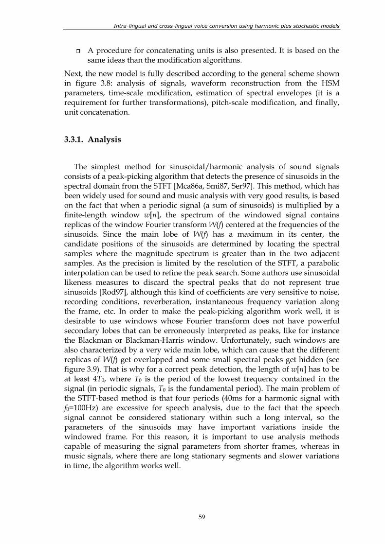
Intra-lingual and cross-lingual voice conversion using harmonic plus stochastic models
59
A procedure for concatenating units is also presented. It is based on the same ideas than the modification algorithms.
Next, the new model is fully described according to the general scheme shown in figure 3.8: analysis of signals, waveform reconstruction from the HSM parameters, time-scale modification, estimation of spectral envelopes (it is a requirement for further transformations), pitch-scale modification, and finally, unit concatenation.
3.3.1. Analysis
The simplest method for sinusoidal/harmonic analysis of sound signals consists of a peak-picking algorithm that detects the presence of sinusoids in the spectral domain from the STFT [Mca86a, Smi87, Ser97]. This method, which has been widely used for sound and music analysis with very good results, is based on the fact that when a periodic signal (a sum of sinusoids) is multiplied by a finite-length window w[n], the spectrum of the windowed signal contains replicas of the window Fourier transform W(f) centered at the frequencies of the sinusoids. Since the main lobe of W(f) has a maximum in its center, the candidate positions of the sinusoids are determined by locating the spectral samples where the magnitude spectrum is greater than in the two adjacent samples. As the precision is limited by the resolution of the STFT, a parabolic interpolation can be used to refine the peak search. Some authors use sinusoidal likeness measures to discard the spectral peaks that do not represent true sinusoids [Rod97], although this kind of coefficients are very sensitive to noise, recording conditions, reverberation, instantaneous frequency variation along the frame, etc. In order to make the peak-picking algorithm work well, it is desirable to use windows whose Fourier transform does not have powerful secondary lobes that can be erroneously interpreted as peaks, like for instance the Blackman or Blackman-Harris window. Unfortunately, such windows are also characterized by a very wide main lobe, which can cause that the different replicas of W(f) get overlapped and some small spectral peaks get hidden (see figure 3.9). That is why for a correct peak detection, the length of w[n] has to be at least 4T0, where T0 is the period of the lowest frequency contained in the signal (in periodic signals, T0 is the fundamental period). The main problem of the STFT-based method is that four periods (40ms for a harmonic signal with f0=100Hz) are excessive for speech analysis, due to the fact that the speech signal cannot be considered stationary within such a long interval, so the parameters of the sinusoids may have important variations inside the windowed frame. For this reason, it is important to use analysis methods capable of measuring the signal parameters from shorter frames, whereas in music signals, where there are long stationary segments and slower variations in time, the algorithm works well.
Chapter 3. Flexible harmonic plus stochastic speech model
60
Figure 3.9: spectrum of a stationary harmonic synthetic signal with f0=102 Hz. a) Two periods
using Blackman-Harris window. b) Four periods using Blackman-Harris window. c) Two periods using rectangular window. d) Four periods using rectangular window.
In previous works it was shown that it is possible to measure the amplitudes and phases of the sinusoids from a two-period-length windowed frame through a least squares optimization, assuming that the pitch has been previously estimated with enough accuracy. This can be done either in the time domain [Sty96] or in the frequency domain [Dep97].
In the time-domain implementation, for a given frame k of length N+1 containing L harmonics, the error to be minimized can be expressed as
[ ] [ ] [ ]( ) [ ] ∑∑−=−=
=−⋅=L
Ll
njlwlh
N
Nnh eCnsnsnsnw 0 ,
2
2
22ε (3.16)
where s[n] is the real speech signal, Cl are the complex amplitudes (which verify the condition C-l=Cl*) and w[n] is a certain weighting function whose maximum is located at the frame center. For simplicity, the frame center has been placed at n=0 and the super-index (k) has been omitted. The vector sh that contains the samples of the harmonic frame can be expressed as
( ) ( ) ( ) ( )
( ) ( ) ( ) ( )
( ) ( ) ( ) ( )
=
=⋅=∗−
∗
−−−
+−+−−−+−−
−−−−−−
L
L
L
NjLwNwLjNjLw
NjLwNwLjNjLw
NjLwNwLjNjLw
h
C
CC
eee
eeeeee
M
K
MOMM
K
K
1
2212
1212112
2212
000
000
000
, xBxBs (3.17)
The weighting function can be expressed by means of a square diagonal matrix W where the diagonal elements are the samples w[-N/2], …, w[N/2]. Thus, the final equation system to be optimized is the following.
( ) WsWBxWBWBWsWBx HHopt
HH =⇒= (3.18)
where s is the vector containing the speech samples of the current frame. The main advantage of the time-domain implementation is that (BHWHWB) is a Toeplitz matrix, so the solution can be reached efficiently by Levinson’s algorithm. Once xopt is calculated, the amplitudes and phases of the harmonics are given by
Intra-lingual and cross-lingual voice conversion using harmonic plus stochastic models
61
llllll CCCCA −− −==== argarg ,22 ϕ (3.19)
[Lar93] includes a more complete version of the method in which a similar optimization leads to the estimation of the complex slopes of the complex amplitudes along the frame, which can be used also for the refinement of the pitch estimate.
In the frequency domain [Dep97], the measured short-time spectrum can be approximated as
( ) ( ) ( )( )
( ) ( )( ) ( ) ( )( )[ ]∑
∑
=
=
−
+−−+++−=
=++−≅
L
lll
jllllll
L
ll
jl
jl
ffWffWAffWffWA
ffWeffWeAfS ll
122
1
121
sincos ϕϕ
ϕϕ
(3.20)
where fl corresponds to lf0. This can be expressed as
SxH =⋅ (3.21)
where H is the matrix whose lth column is given by the spectrum Hl(f), defined as
( ) ( ) ( )( )( ) ( ) ( )( )ll
jlL
lll
ffWffWfH
ffWffWfH
+−−=
++−=
+ 2
21
(3.22)
S contains the STFT of the current frame, and x is defined as
[ ]TLLLL AAAA ϕϕϕϕ sinsincoscos 1111 KK=x (3.23)
The optimum x is given by
( ) SHHHx HHopt
1−= (3.24)
The amplitudes and phases are easily extracted from xopt. In both, the time-domain and the frequency-domain implementation, a first estimate of the pitch has to be available before the optimization. In principle, any of the existing methods for pitch detection can be used for this task. In this case, the modified autocorrelation method presented in [Boe93] was chosen. Several objective experiments carried out with natural speech signals showed that both the time-domain and the frequency-domain implementations have a similar performance in terms of accuracy. Both methods work well in a pitch-asynchronous context for a two-period-length analysis window, regardless of the position of the analysis instants within the signal periods. Therefore, the only difference between them is that the frequency-domain implementation is characterized by a higher computational load. It can be concluded that the time-domain method is better than the frequency-domain method. It was also checked that the ABS-OLA technique proposed in [Geo97], which optimizes the error for one only sinusoidal component at a time until the whole analysis band is covered, led to less accurate results.
Chapter 3. Flexible harmonic plus stochastic speech model
62
Once the sinusoidal part of the signal has been measured, for the analysis to be completed, the stochastic component has to be isolated and parameterized. There are two ways of doing this:
1) By taking the error of the sinusoidal estimation as stochastic component. This error, which can be calculated either in the time-domain or in the frequency-domain, would be then analyzed so that the stochastic component is characterized locally at each analysis frame.
2) By interpolating and regenerating the deterministic component from the parameters measured along the signal, and then subtracting it from the original waveform. The resulting stochastic signal would be then analyzed frame-by-frame.
The first approach has one main problem: the methods for optimization of the sinusoidal parameters assume that the signal frequencies and amplitudes are steady. On the contrary, the second approach allows imitating the real evolution of the amplitudes, frequencies and phases, so in principle the effects of the time variation are minimized. Indeed, comparative experiments confirm that the energy of the resulting stochastic component is lower when the second strategy is followed. In order to examine the implementation details, let us consider the analysis frames k and k+1, centered at n=kN and n=(k+1)N, respectively. The instantaneous amplitude Al[n] and phase φl[n] of the lth harmonic can be interpolated between the frame centers using the equations proposed by McAulay and Quatieri in [Mca86a]:
[ ] ( )[ ]
NmdcmbmammkNAAAmkNA
l
kl
klN
mkll <≤
+++=+
−+=+ +
023
)()1()(
ϕ (3.25)
(3.26)
The phase polynomial satisfies the following conditions:
[ ] ( )[ ][ ] ( )[ ] )1()(
)1()(
1 ,,21 ,
+
+
=+=
+=+=k
llk
ll
kll
kll
wNkwkNMNkkN
ϕϕ
πϕϕϕϕ
&& (3.27)
The frequencies are integer multiples of the pitch w0(k). The phase unwrapping parameter M is the integer number that makes the instantaneous frequency maximally smooth:
[ ]( )( )
( ) ( )[ ] 2)()1()1()()(
21
1 2
round
,minarground
Nkl
kl
kl
kl
kl
Nk
kN lM
wwNw
dnMnM
−+−+=
=
=
++
+
∫ϕϕ
ϕ
π
&& (3.28)
Therefore, the polynomial coefficients are:
( ) ( )( ) ( ))()1(1)()()1(2
)()1(1)()()1(3
)()(
23
2
2
2
kl
klN
kl
kl
klN
kl
klN
kl
kl
klN
kl
kl
wwNwMa
wwNwMbwcd
−+−−+=
−−−−+=
==
++−
++
ϕπϕ
ϕπϕ
ϕ
(3.29)
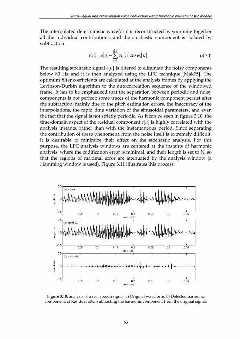
Intra-lingual and cross-lingual voice conversion using harmonic plus stochastic models
63
The interpolated deterministic waveform is reconstructed by summing together all the individual contributions, and the stochastic component is isolated by subtraction.
[ ] [ ] [ ] [ ][ ]
∑=
−=nL
lll nnAnsne
1cosϕ (3.30)
The resulting stochastic signal e[n] is filtered to eliminate the noisy components below 80 Hz and it is then analyzed using the LPC technique [Mak75]. The optimum filter coefficients are calculated at the analysis frames by applying the Levinson-Durbin algorithm to the autocorrelation sequence of the windowed frame. It has to be emphasized that the separation between periodic and noisy components is not perfect: some traces of the harmonic component persist after the subtraction, mainly due to the pitch estimation errors, the inaccuracy of the interpolations, the rapid time variation of the sinusoidal parameters, and even the fact that the signal is not strictly periodic. As it can be seen in figure 3.10, the time-domain aspect of the residual component e[n] is highly correlated with the analysis instants, rather than with the instantaneous period. Since separating the contribution of these phenomena from the noise itself is extremely difficult, it is desirable to minimize their effect on the stochastic analysis. For this purpose, the LPC analysis windows are centered at the instants of harmonic analysis, where the codification error is minimal, and their length is set to N, so that the regions of maximal error are attenuated by the analysis window (a Hamming window is used). Figure 3.11 illustrates this process.
Figure 3.10: analysis of a real speech signal. a) Original waveform. b) Detected harmonic
component. c) Residual after subtracting the harmonic component from the original signal.
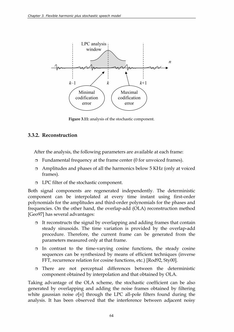
Chapter 3. Flexible harmonic plus stochastic speech model
64
Figure 3.11: analysis of the stochastic component.
3.3.2. Reconstruction
After the analysis, the following parameters are available at each frame:
Fundamental frequency at the frame center (0 for unvoiced frames).
Amplitudes and phases of all the harmonics below 5 KHz (only at voiced frames).
LPC filter of the stochastic component.
Both signal components are regenerated independently. The deterministic component can be interpolated at every time instant using first-order polynomials for the amplitudes and third-order polynomials for the phases and frequencies. On the other hand, the overlap-add (OLA) reconstruction method [Geo97] has several advantages:
It reconstructs the signal by overlapping and adding frames that contain steady sinusoids. The time variation is provided by the overlap-add procedure. Therefore, the current frame can be generated from the parameters measured only at that frame.
In contrast to the time-varying cosine functions, the steady cosine sequences can be synthesized by means of efficient techniques (inverse FFT, recurrence relation for cosine functions, etc.) [Rod92, Sty00].
There are not perceptual differences between the deterministic component obtained by interpolation and that obtained by OLA.
Taking advantage of the OLA scheme, the stochastic coefficient can be also generated by overlapping and adding the noise frames obtained by filtering white gaussian noise σ[n] through the LPC all-pole filters found during the analysis. It has been observed that the interference between adjacent noisy
n
k k+1k–1
LPC analysis window
Minimal codification
error
Maximal codification
error
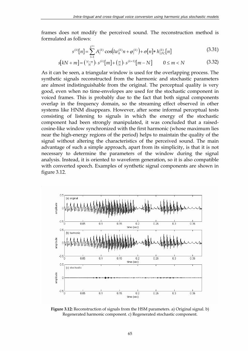
Intra-lingual and cross-lingual voice conversion using harmonic plus stochastic models
65
frames does not modify the perceived sound. The reconstruction method is formulated as follows:
[ ] ( ) [ ] [ ]nhnnlwAns kLPC
L
l
kl
kkl
kk
)(
1
)()(0
)()()(
cos ∗++= ∑=
σϕ
[ ] ( ) [ ] ( ) [ ] NmNmsmsmkNs kNmk
NmN <≤−⋅+⋅=+ +− 0 )1()(
(3.31)
(3.32)
As it can be seen, a triangular window is used for the overlapping process. The synthetic signals reconstructed from the harmonic and stochastic parameters are almost indistinguishable from the original. The perceptual quality is very good, even when no time-envelopes are used for the stochastic component in voiced frames. This is probably due to the fact that both signal components overlap in the frequency domain, so the streaming effect observed in other systems like HNM disappears. However, after some informal perceptual tests consisting of listening to signals in which the energy of the stochastic component had been strongly manipulated, it was concluded that a raised-cosine-like window synchronized with the first harmonic (whose maximum lies near the high-energy regions of the period) helps to maintain the quality of the signal without altering the characteristics of the perceived sound. The main advantage of such a simple approach, apart from its simplicity, is that it is not necessary to determine the parameters of the window during the signal analysis. Instead, it is oriented to waveform generation, so it is also compatible with converted speech. Examples of synthetic signal components are shown in figure 3.12.
Figure 3.12: Reconstruction of signals from the HSM parameters. a) Original signal. b)
Regenerated harmonic component. c) Regenerated stochastic component.
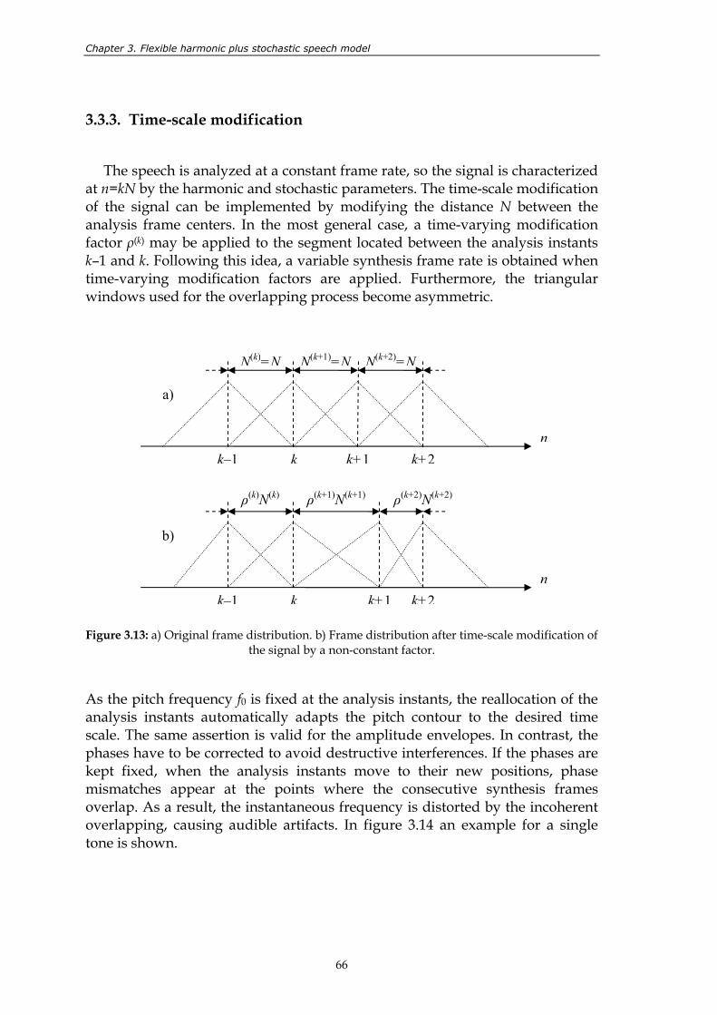
Chapter 3. Flexible harmonic plus stochastic speech model
66
3.3.3. Time-scale modification
The speech is analyzed at a constant frame rate, so the signal is characterized at n=kN by the harmonic and stochastic parameters. The time-scale modification of the signal can be implemented by modifying the distance N between the analysis frame centers. In the most general case, a time-varying modification factor ρ(k) may be applied to the segment located between the analysis instants k–1 and k. Following this idea, a variable synthesis frame rate is obtained when time-varying modification factors are applied. Furthermore, the triangular windows used for the overlapping process become asymmetric.
Figure 3.13: a) Original frame distribution. b) Frame distribution after time-scale modification of
the signal by a non-constant factor.
As the pitch frequency f0 is fixed at the analysis instants, the reallocation of the analysis instants automatically adapts the pitch contour to the desired time scale. The same assertion is valid for the amplitude envelopes. In contrast, the phases have to be corrected to avoid destructive interferences. If the phases are kept fixed, when the analysis instants move to their new positions, phase mismatches appear at the points where the consecutive synthesis frames overlap. As a result, the instantaneous frequency is distorted by the incoherent overlapping, causing audible artifacts. In figure 3.14 an example for a single tone is shown.
kk–1 k+1 k+2
N(k)=N N(k+1)=N N(k+2)=N
n
kk–1 k+1 k+2
ρ(k)N(k) ρ(k+2)N(k+2)
n
ρ(k+1)N(k+1)
a)
b)
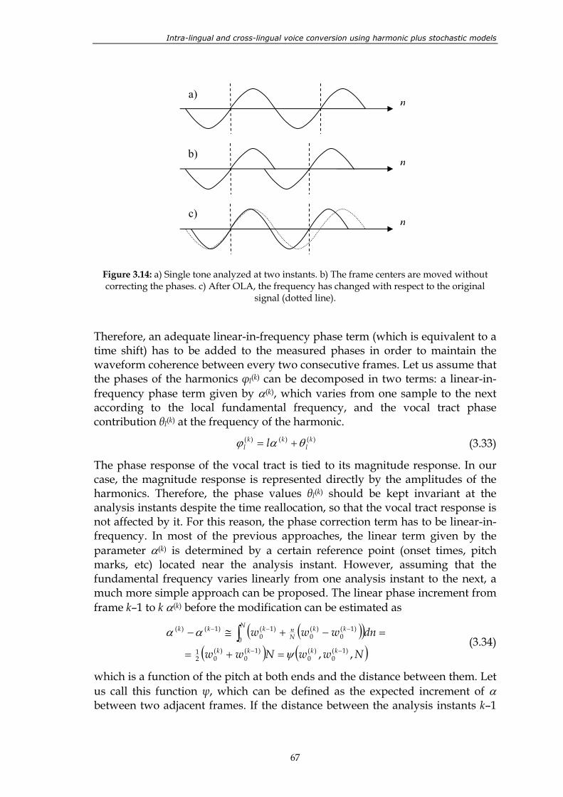
Intra-lingual and cross-lingual voice conversion using harmonic plus stochastic models
67
Figure 3.14: a) Single tone analyzed at two instants. b) The frame centers are moved without correcting the phases. c) After OLA, the frequency has changed with respect to the original
signal (dotted line).
Therefore, an adequate linear-in-frequency phase term (which is equivalent to a time shift) has to be added to the measured phases in order to maintain the waveform coherence between every two consecutive frames. Let us assume that the phases of the harmonics φl(k) can be decomposed in two terms: a linear-in-frequency phase term given by α(k), which varies from one sample to the next according to the local fundamental frequency, and the vocal tract phase contribution θl(k) at the frequency of the harmonic.
)()()( kl
kkl l θαϕ += (3.33)
The phase response of the vocal tract is tied to its magnitude response. In our case, the magnitude response is represented directly by the amplitudes of the harmonics. Therefore, the phase values θl(k) should be kept invariant at the analysis instants despite the time reallocation, so that the vocal tract response is not affected by it. For this reason, the phase correction term has to be linear-in-frequency. In most of the previous approaches, the linear term given by the parameter α(k) is determined by a certain reference point (onset times, pitch marks, etc) located near the analysis instant. However, assuming that the fundamental frequency varies linearly from one analysis instant to the next, a much more simple approach can be proposed. The linear phase increment from frame k–1 to k α(k) before the modification can be estimated as
( )( )( ) ( )NwwNww
dnwwwkkkk
N kkNnkkk
,, )1(0
)(0
)1(0
)(02
1
0
)1(0
)(0
)1(0
)1()(
−−
−−−
=+=
=−+≅− ∫ψ
αα (3.34)
which is a function of the pitch at both ends and the distance between them. Let us call this function ψ, which can be defined as the expected increment of α between two adjacent frames. If the distance between the analysis instants k–1
n
n
n
a)
b)
c)
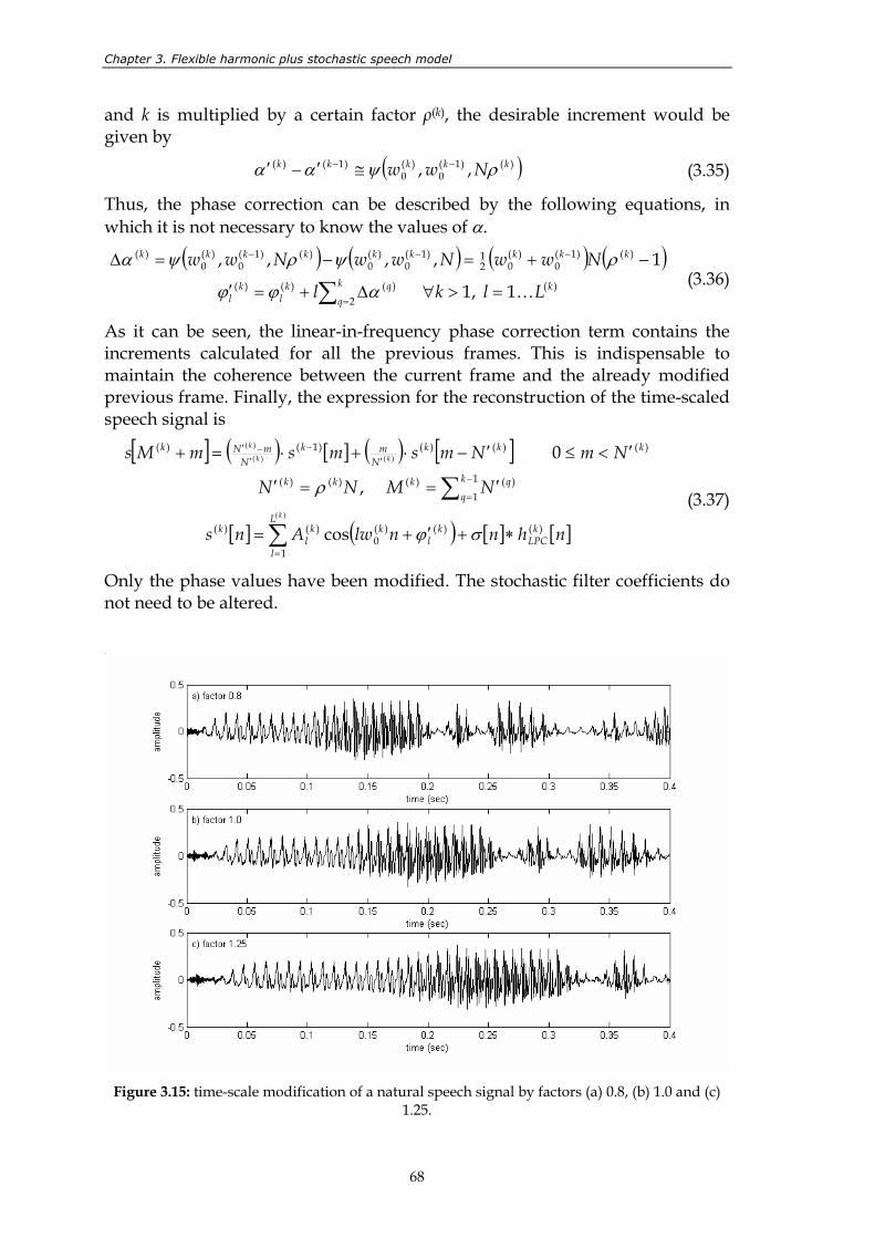
Chapter 3. Flexible harmonic plus stochastic speech model
68
and k is multiplied by a certain factor ρ(k), the desirable increment would be given by
( ))()1(0
)(0
)1()( ,, kkkkk Nww ρψαα −− ≅′−′ (3.35)
Thus, the phase correction can be described by the following equations, in which it is not necessary to know the values of α.
( ) ( ) ( ) ( ))(
2)()()(
)()1(0
)(02
1)1(0
)(0
)()1(0
)(0
)(
1 ,1
1,,,,kk
qqk
lk
l
kkkkkkkkk
Llkl
NwwNwwNww
K=>∀∆+=′
−+=−=∆
∑ =
−−−
αϕϕ
ρψρψα (3.36)
As it can be seen, the linear-in-frequency phase correction term contains the increments calculated for all the previous frames. This is indispensable to maintain the coherence between the current frame and the already modified previous frame. Finally, the expression for the reconstruction of the time-scaled speech signal is
[ ] ( ) [ ] ( ) [ ]
[ ] ( ) [ ] [ ]nhnnlwAns
NMNN
NmNmsmsmMs
kLPC
L
l
kl
kkl
k
k
qqkkk
kkkN
mkN
mNk
k
kk
k
)(
1
)()(0
)()(
1
1)()()()(
)()()()1()(
)(
)()(
)(
cos
,
0
∗+′+=
′==′
′<≤′−⋅+⋅=+
∑
∑
=
−
=
′−
′−′
σϕ
ρ (3.37)
Only the phase values have been modified. The stochastic filter coefficients do not need to be altered.
Figure 3.15: time-scale modification of a natural speech signal by factors (a) 0.8, (b) 1.0 and (c)
1.25.
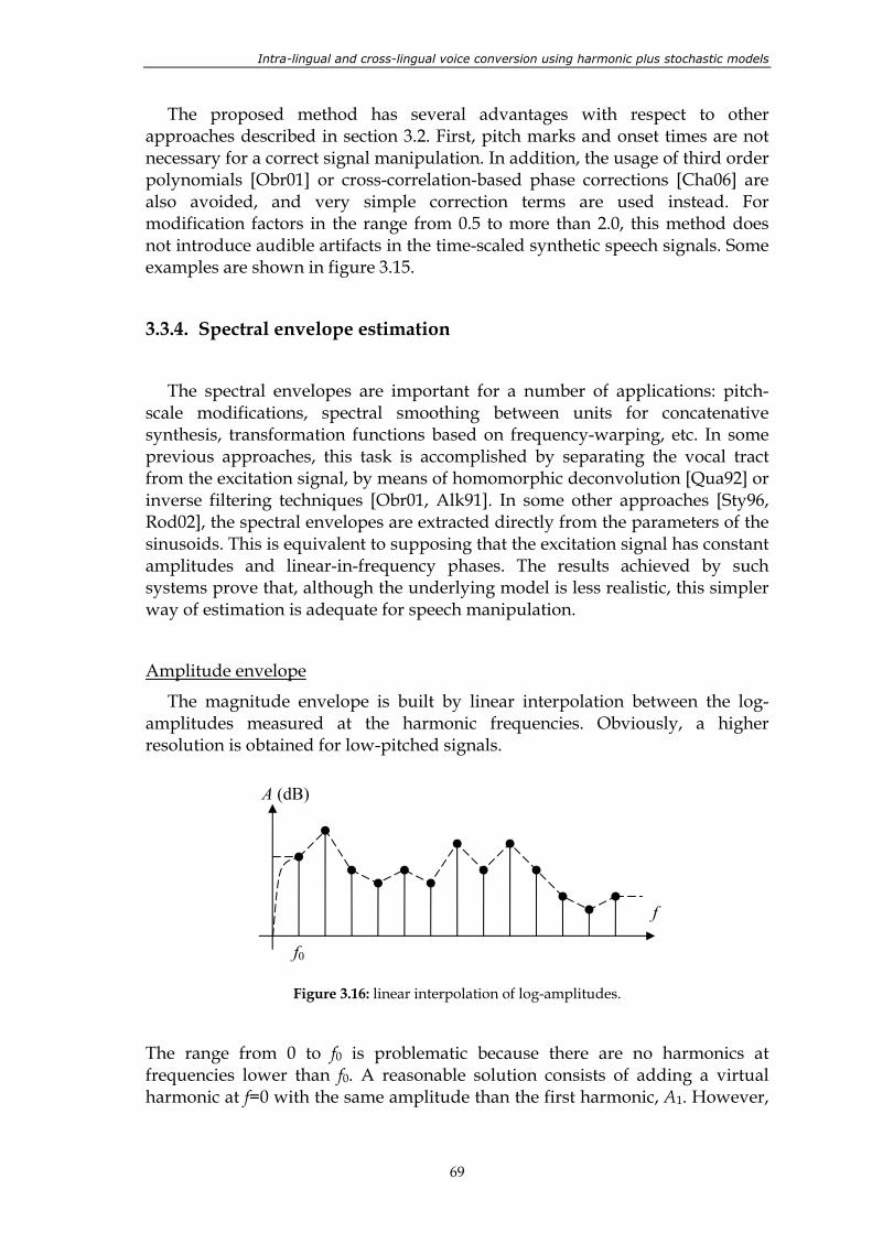
Intra-lingual and cross-lingual voice conversion using harmonic plus stochastic models
69
The proposed method has several advantages with respect to other approaches described in section 3.2. First, pitch marks and onset times are not necessary for a correct signal manipulation. In addition, the usage of third order polynomials [Obr01] or cross-correlation-based phase corrections [Cha06] are also avoided, and very simple correction terms are used instead. For modification factors in the range from 0.5 to more than 2.0, this method does not introduce audible artifacts in the time-scaled synthetic speech signals. Some examples are shown in figure 3.15.
3.3.4. Spectral envelope estimation
The spectral envelopes are important for a number of applications: pitch-scale modifications, spectral smoothing between units for concatenative synthesis, transformation functions based on frequency-warping, etc. In some previous approaches, this task is accomplished by separating the vocal tract from the excitation signal, by means of homomorphic deconvolution [Qua92] or inverse filtering techniques [Obr01, Alk91]. In some other approaches [Sty96, Rod02], the spectral envelopes are extracted directly from the parameters of the sinusoids. This is equivalent to supposing that the excitation signal has constant amplitudes and linear-in-frequency phases. The results achieved by such systems prove that, although the underlying model is less realistic, this simpler way of estimation is adequate for speech manipulation.
Amplitude envelope
The magnitude envelope is built by linear interpolation between the log-amplitudes measured at the harmonic frequencies. Obviously, a higher resolution is obtained for low-pitched signals.
Figure 3.16: linear interpolation of log-amplitudes.
The range from 0 to f0 is problematic because there are no harmonics at frequencies lower than f0. A reasonable solution consists of adding a virtual harmonic at f=0 with the same amplitude than the first harmonic, A1. However,
A (dB)
f
f0
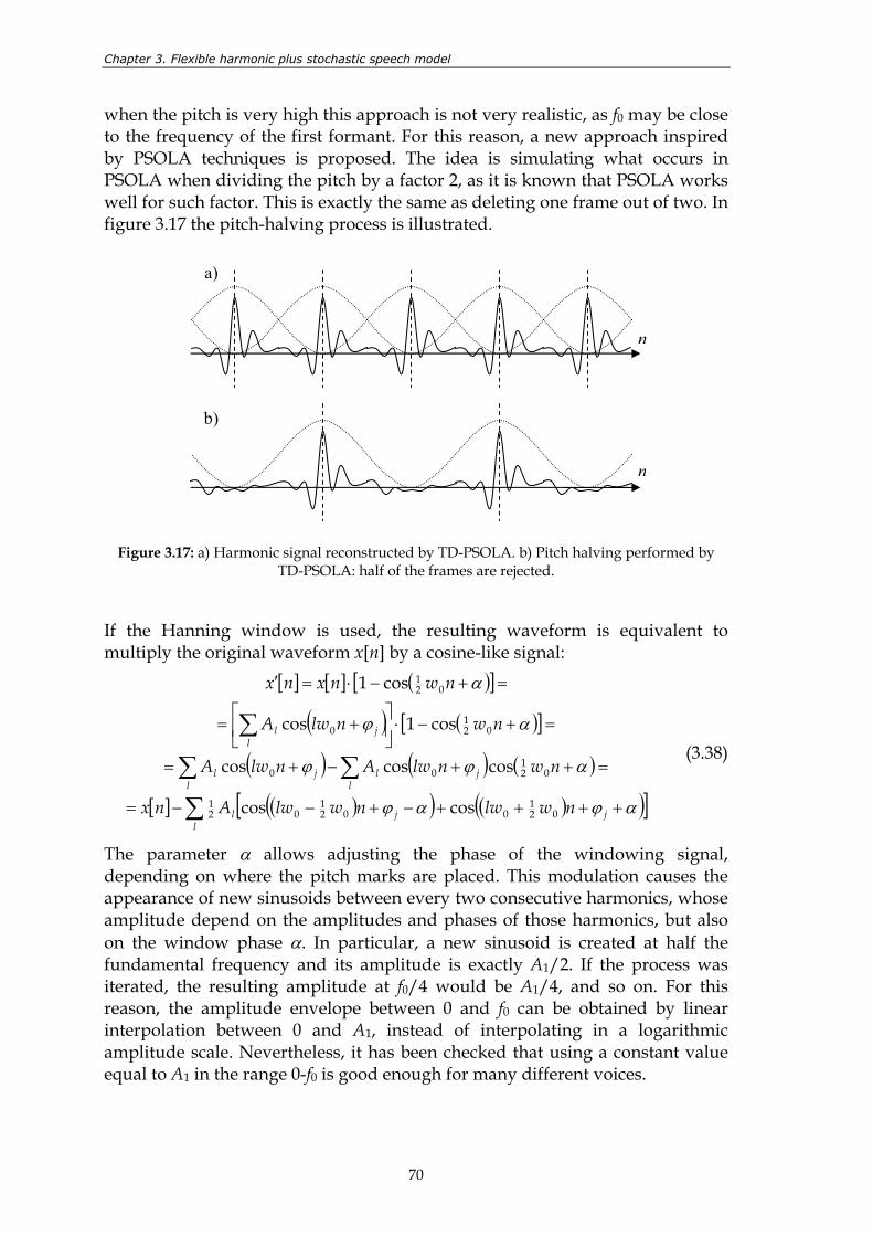
Chapter 3. Flexible harmonic plus stochastic speech model
70
when the pitch is very high this approach is not very realistic, as f0 may be close to the frequency of the first formant. For this reason, a new approach inspired by PSOLA techniques is proposed. The idea is simulating what occurs in PSOLA when dividing the pitch by a factor 2, as it is known that PSOLA works well for such factor. This is exactly the same as deleting one frame out of two. In figure 3.17 the pitch-halving process is illustrated.
Figure 3.17: a) Harmonic signal reconstructed by TD-PSOLA. b) Pitch halving performed by
TD-PSOLA: half of the frames are rejected.
If the Hanning window is used, the resulting waveform is equivalent to multiply the original waveform x[n] by a cosine-like signal:
[ ] [ ] ( )[ ]
( ) ( )[ ]
( ) ( ) ( )
[ ] ( )( ) ( )( )[ ]∑
∑∑
∑
++++−+−−=
=++−+=
=+−⋅
+=
=+−⋅=′
ljjl
ljl
ljl
ljl
nwlwnwlwAnx
nwnlwAnlwA
nwnlwA
nwnxnx
αϕαϕ
αϕϕ
αϕ
α
021
0021
021
021
00
021
0
021
coscos
coscoscos
cos1cos
cos1
(3.38)
The parameter α allows adjusting the phase of the windowing signal, depending on where the pitch marks are placed. This modulation causes the appearance of new sinusoids between every two consecutive harmonics, whose amplitude depend on the amplitudes and phases of those harmonics, but also on the window phase α. In particular, a new sinusoid is created at half the fundamental frequency and its amplitude is exactly A1/2. If the process was iterated, the resulting amplitude at f0/4 would be A1/4, and so on. For this reason, the amplitude envelope between 0 and f0 can be obtained by linear interpolation between 0 and A1, instead of interpolating in a logarithmic amplitude scale. Nevertheless, it has been checked that using a constant value equal to A1 in the range 0-f0 is good enough for many different voices.
n
n
a)
b)
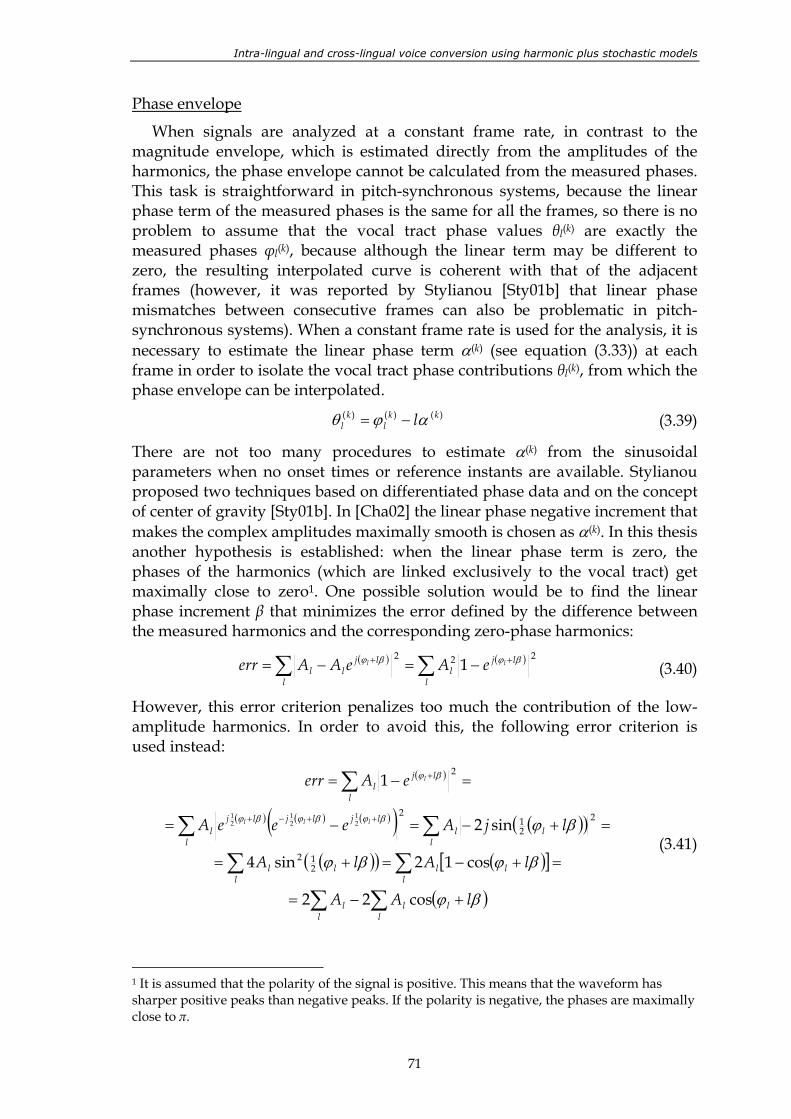
Intra-lingual and cross-lingual voice conversion using harmonic plus stochastic models
71
Phase envelope
When signals are analyzed at a constant frame rate, in contrast to the magnitude envelope, which is estimated directly from the amplitudes of the harmonics, the phase envelope cannot be calculated from the measured phases. This task is straightforward in pitch-synchronous systems, because the linear phase term of the measured phases is the same for all the frames, so there is no problem to assume that the vocal tract phase values θl(k) are exactly the measured phases φl(k), because although the linear term may be different to zero, the resulting interpolated curve is coherent with that of the adjacent frames (however, it was reported by Stylianou [Sty01b] that linear phase mismatches between consecutive frames can also be problematic in pitch-synchronous systems). When a constant frame rate is used for the analysis, it is necessary to estimate the linear phase term α(k) (see equation (3.33)) at each frame in order to isolate the vocal tract phase contributions θl(k), from which the phase envelope can be interpolated.
)()()( kkl
kl lαϕθ −= (3.39)
There are not too many procedures to estimate α(k) from the sinusoidal parameters when no onset times or reference instants are available. Stylianou proposed two techniques based on differentiated phase data and on the concept of center of gravity [Sty01b]. In [Cha02] the linear phase negative increment that makes the complex amplitudes maximally smooth is chosen as α(k). In this thesis another hypothesis is established: when the linear phase term is zero, the phases of the harmonics (which are linked exclusively to the vocal tract) get maximally close to zero1. One possible solution would be to find the linear phase increment β that minimizes the error defined by the difference between the measured harmonics and the corresponding zero-phase harmonics:
( ) ( )∑∑ ++ −=−=l
ljl
l
ljll
ll eAeAAerr222
1 βϕβϕ (3.40)
However, this error criterion penalizes too much the contribution of the low-amplitude harmonics. In order to avoid this, the following error criterion is used instead:
( )
( ) ( ) ( )( ) ( )( )
( )( ) ( )[ ]
( )∑∑
∑∑
∑∑
∑
+−=
=+−=+=
=+−=−=
=−=
++−+
+
lll
ll
lll
lll
lll
l
ljljljl
l
ljl
lAA
lAlA
ljAeeeA
eAerr
lll
l
βϕ
βϕβϕ
βϕβϕβϕβϕ
βϕ
cos22
cos12sin4
sin2
1
212
221
2
2
21
21
21
(3.41)
1 It is assumed that the polarity of the signal is positive. This means that the waveform has sharper positive peaks than negative peaks. If the polarity is negative, the phases are maximally close to π.
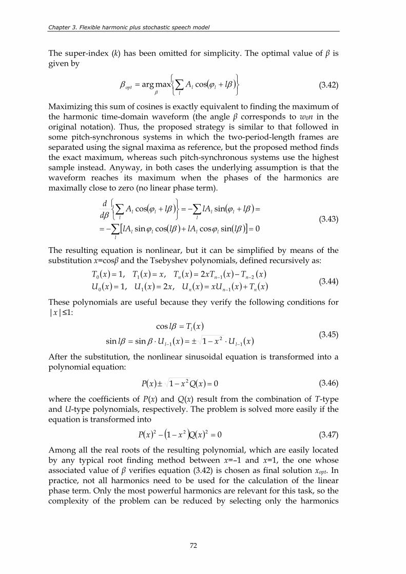
Chapter 3. Flexible harmonic plus stochastic speech model
72
The super-index (k) has been omitted for simplicity. The optimal value of β is given by
( )
+= ∑l
llopt lA βϕββ
cosmaxarg (3.42)
Maximizing this sum of cosines is exactly equivalent to finding the maximum of the harmonic time-domain waveform (the angle β corresponds to w0n in the original notation). Thus, the proposed strategy is similar to that followed in some pitch-synchronous systems in which the two-period-length frames are separated using the signal maxima as reference, but the proposed method finds the exact maximum, whereas such pitch-synchronous systems use the highest sample instead. Anyway, in both cases the underlying assumption is that the waveform reaches its maximum when the phases of the harmonics are maximally close to zero (no linear phase term).
( ) ( )
( ) ( )[ ] 0sincoscossin
sincos
=+−=
=+−=
+
∑
∑∑
lllll
lll
lll
llAllA
llAlAdd
βϕβϕ
βϕβϕβ (3.43)
The resulting equation is nonlinear, but it can be simplified by means of the substitution x=cosβ and the Tsebyshev polynomials, defined recursively as:
( ) ( ) ( ) ( ) ( )( ) ( ) ( ) ( ) ( )xTxxUxUxxUxU
xTxxTxTxxTxT
nnn
nnn
+===−===
−
−−
110
2110
,2,12,,1
(3.44)
These polynomials are useful because they verify the following conditions for |x|≤1:
( )( ) ( )xUxxUl
xTl
ll
l
12
1 1sinsin
cos
−− ⋅−±=⋅=
=
ββ
β (3.45)
After the substitution, the nonlinear sinusoidal equation is transformed into a polynomial equation:
( ) ( ) 01 2 =−± xQxxP (3.46)
where the coefficients of P(x) and Q(x) result from the combination of T-type and U-type polynomials, respectively. The problem is solved more easily if the equation is transformed into
( ) ( ) ( ) 01 222 =−− xQxxP (3.47)
Among all the real roots of the resulting polynomial, which are easily located by any typical root finding method between x=–1 and x=1, the one whose associated value of β verifies equation (3.42) is chosen as final solution xopt. In practice, not all harmonics need to be used for the calculation of the linear phase term. Only the most powerful harmonics are relevant for this task, so the complexity of the problem can be reduced by selecting only the harmonics
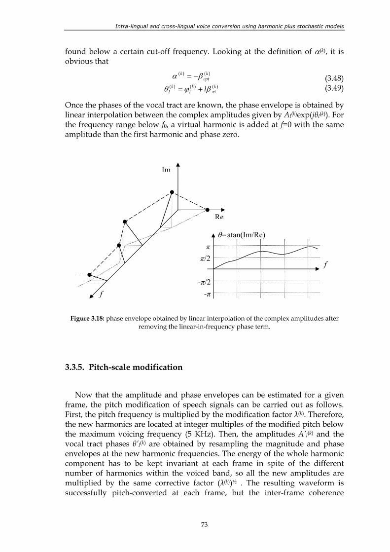
Intra-lingual and cross-lingual voice conversion using harmonic plus stochastic models
73
found below a certain cut-off frequency. Looking at the definition of α(k), it is obvious that
)()( kopt
k βα −= )()()( kk
lk
l optlβϕθ += (3.48) (3.49)
Once the phases of the vocal tract are known, the phase envelope is obtained by linear interpolation between the complex amplitudes given by Al(k)exp(jθl(k)). For the frequency range below f0, a virtual harmonic is added at f=0 with the same amplitude than the first harmonic and phase zero.
Figure 3.18: phase envelope obtained by linear interpolation of the complex amplitudes after
removing the linear-in-frequency phase term.
3.3.5. Pitch-scale modification
Now that the amplitude and phase envelopes can be estimated for a given frame, the pitch modification of speech signals can be carried out as follows. First, the pitch frequency is multiplied by the modification factor λ(k). Therefore, the new harmonics are located at integer multiples of the modified pitch below the maximum voicing frequency (5 KHz). Then, the amplitudes A’l(k) and the vocal tract phases θ’l(k) are obtained by resampling the magnitude and phase envelopes at the new harmonic frequencies. The energy of the whole harmonic component has to be kept invariant at each frame in spite of the different number of harmonics within the voiced band, so all the new amplitudes are multiplied by the same corrective factor (λ(k))½ . The resulting waveform is successfully pitch-converted at each frame, but the inter-frame coherence
Re
f
Im
f
θ=atan(Im/Re)π
-π
π/2
-π/2
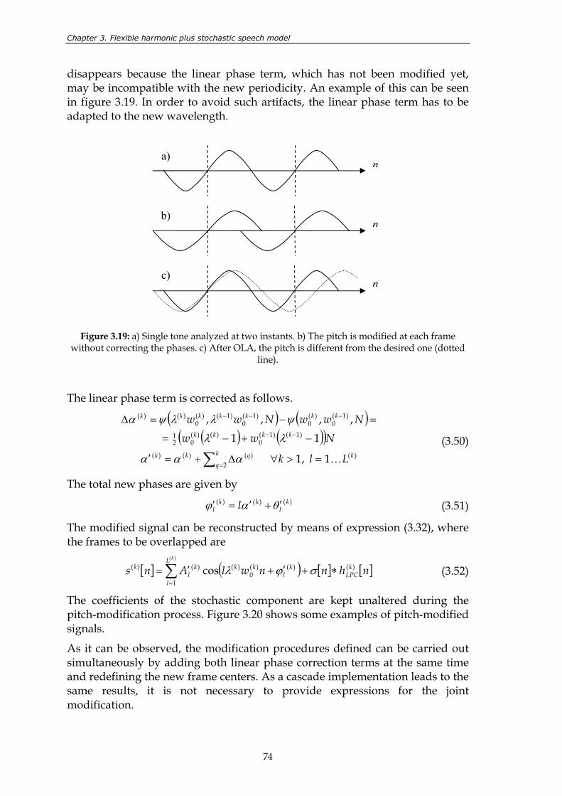
Chapter 3. Flexible harmonic plus stochastic speech model
74
disappears because the linear phase term, which has not been modified yet, may be incompatible with the new periodicity. An example of this can be seen in figure 3.19. In order to avoid such artifacts, the linear phase term has to be adapted to the new wavelength.
Figure 3.19: a) Single tone analyzed at two instants. b) The pitch is modified at each frame
without correcting the phases. c) After OLA, the pitch is different from the desired one (dotted line).
The linear phase term is corrected as follows.
( ) ( )( ) ( )( )
)(2
)()()(
)1()1(0
)()(02
1
)1(0
)(0
)1(0
)1()(0
)()(
1 ,1
11,,,,
kk
qqkk
kkkk
kkkkkkk
Llk
NwwNwwNww
K=>∀∆+=′
−+−=
=−=∆
∑ =
−−
−−−
ααα
λλ
ψλλψα
(3.50)
The total new phases are given by )()()( k
lkk
l l θαϕ ′+′=′ (3.51)
The modified signal can be reconstructed by means of expression (3.32), where the frames to be overlapped are
[ ] ( ) [ ] [ ]nhnnwlAns kLPC
L
l
kl
kkkl
kk
)(
1
)()(0
)()()()(
cos ∗+′+′= ∑=
σϕλ (3.52)
The coefficients of the stochastic component are kept unaltered during the pitch-modification process. Figure 3.20 shows some examples of pitch-modified signals.
As it can be observed, the modification procedures defined can be carried out simultaneously by adding both linear phase correction terms at the same time and redefining the new frame centers. As a cascade implementation leads to the same results, it is not necessary to provide expressions for the joint modification.
n
n
n
a)
b)
c)
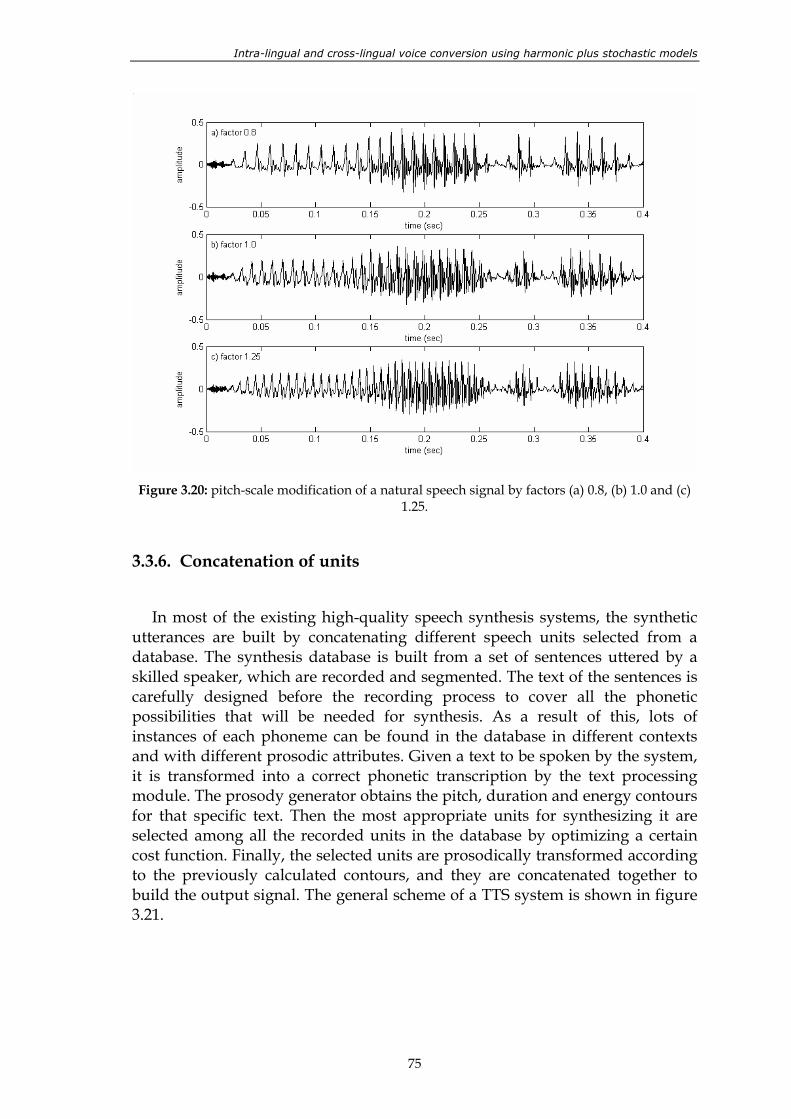
Intra-lingual and cross-lingual voice conversion using harmonic plus stochastic models
75
Figure 3.20: pitch-scale modification of a natural speech signal by factors (a) 0.8, (b) 1.0 and (c)
1.25.
3.3.6. Concatenation of units
In most of the existing high-quality speech synthesis systems, the synthetic utterances are built by concatenating different speech units selected from a database. The synthesis database is built from a set of sentences uttered by a skilled speaker, which are recorded and segmented. The text of the sentences is carefully designed before the recording process to cover all the phonetic possibilities that will be needed for synthesis. As a result of this, lots of instances of each phoneme can be found in the database in different contexts and with different prosodic attributes. Given a text to be spoken by the system, it is transformed into a correct phonetic transcription by the text processing module. The prosody generator obtains the pitch, duration and energy contours for that specific text. Then the most appropriate units for synthesizing it are selected among all the recorded units in the database by optimizing a certain cost function. Finally, the selected units are prosodically transformed according to the previously calculated contours, and they are concatenated together to build the output signal. The general scheme of a TTS system is shown in figure 3.21.
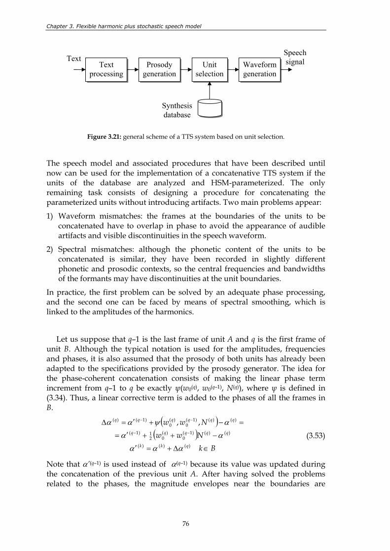
Chapter 3. Flexible harmonic plus stochastic speech model
76
Figure 3.21: general scheme of a TTS system based on unit selection.
The speech model and associated procedures that have been described until now can be used for the implementation of a concatenative TTS system if the units of the database are analyzed and HSM-parameterized. The only remaining task consists of designing a procedure for concatenating the parameterized units without introducing artifacts. Two main problems appear:
1) Waveform mismatches: the frames at the boundaries of the units to be concatenated have to overlap in phase to avoid the appearance of audible artifacts and visible discontinuities in the speech waveform.
2) Spectral mismatches: although the phonetic content of the units to be concatenated is similar, they have been recorded in slightly different phonetic and prosodic contexts, so the central frequencies and bandwidths of the formants may have discontinuities at the unit boundaries.
In practice, the first problem can be solved by an adequate phase processing, and the second one can be faced by means of spectral smoothing, which is linked to the amplitudes of the harmonics.
Let us suppose that q–1 is the last frame of unit A and q is the first frame of unit B. Although the typical notation is used for the amplitudes, frequencies and phases, it is also assumed that the prosody of both units has already been adapted to the specifications provided by the prosody generator. The idea for the phase-coherent concatenation consists of making the linear phase term increment from q–1 to q be exactly ψ(w0(q), w0(q–1), N(q)), where ψ is defined in (3.34). Thus, a linear corrective term is added to the phases of all the frames in B.
( )( )
BkNww
Nww
qkk
qqqqq
qqqqqq
∈∆+=′
−++′=
=−+′=∆−−
−−
)()()(
)()()1(0
)(02
1)1(
)()()1(0
)(0
)1()( ,,
ααα
αα
αψαα
(3.53)
Note that α’(q–1) is used instead of α(q–1) because its value was updated during the concatenation of the previous unit A. After having solved the problems related to the phases, the magnitude envelopes near the boundaries are
Text processing
Prosody generation
Unit selection
Waveform generation
Text Speech signal
Synthesis database
Intra-lingual and cross-lingual voice conversion using harmonic plus stochastic models
77
combined with those of frames q–1 or q for smoothing the spectral discontinuities.
( ) ( ) ( ) ( )( ) ( ) ( )
≥<
−+
−+=′
− qkqk
fAfAfAfA
fAqkkk
qkkkk
)1()()()(
)()()()()(
11
µµ
µµ (3.54)
where µ=1 at the concatenation instant and it decreases linearly until a certain distance from it is reached. Satisfactory perceptual results are obtained if the distance is half the length of the current demiphone. The smoothed amplitudes are calculated by resampling the new weighted envelopes at the harmonic frequencies, and the energy of the harmonic component is preserved by means of a multiplicative factor.
3.4. Validation of the system in a speech synthesis context
Experiments were carried out to validate the new algorithms for prosodic manipulation and concatenation of speech fragments. Speech synthesis by corpus is an adequate context for the validation of the system, because it is a combination between all these tasks. However, building a whole TTS system based on the described model and subjectively evaluating its performance has one main drawback: the opinion of the listeners may be influenced not only by the performance of the waveform generation method, but also by the naturalness of the generated prosody or the accuracy of the selected units. For this reason, in this section a comparative test is carried out between TD-PSOLA and the new technique, using the same TTS engine combined with the two different waveform generators. Most of the existing high-quality speech synthesizers are based on TD-PSOLA, so proving that the new HSM-based techniques outperform TD-PSOLA would confirm that the proposed techniques are suitable for high-quality speech synthesis.
Ogmios is the TTS system of the Universitat Politècnica de Catalunya (UPC), described in appendix A. In the standard version of Ogmios, whose waveform generator is based on TD-PSOLA, the synthetic utterances are built by modifying and concatenating units selected from a corpus. The sequence of units to be concatenated is determined by minimizing a cost function that takes into account the prosodic, phonetic and spectral properties of the units. The quality of the output speech decreases as the prosodic modification factors increase, so the system has been designed to modify only the frames where the required modification factor is higher than a certain threshold, which can be either estimated empirically for each phoneme or specified by the user. In order to better perceive the differences between both waveform generation methods, in this experiment the system was allowed to perform time-scale and pitch-scale modifications in all the speech frames to match the specifications provided by the prosody generation block of Ogmios. Under these conditions, the artifacts
Chapter 3. Flexible harmonic plus stochastic speech model
78
introduced by both methods were more visible for the comparison, whereas the quality of the synthetic sentences was obviously lower. The fact that hybrid systems are preferred rather than TD-PSOLA systems in the described conditions was already proved in [Vio98], so the objective of the current test is just to validate the new implementation of a hybrid system.
A preference test was carried out according to the following experimental setup:
18 listeners participated in the test: 6 speech synthesis experts and 12 volunteers.
4 different voices were used for the experiment: one female voice and one male voice characterized by a large database (around 10 hours of recorded speech), and one female voice and one male voice characterized by a small database (less than 1 hour). When the synthesis database is large, more units with the same phonetic content are available for selection, each of them with its own prosodic aspect, so for a given input sentence to be synthesized, the unit selection process yields a sequence of units whose prosodic contour is closer to the desired values. Therefore, lower modification factors are required and a higher quality is achieved. It is interesting to have an idea on how the database size influences the preference of the listeners.
All the listeners were asked to listen to 17 pairs of synthetic utterances. For each pair, whose components were played in random order, one of the sentences had been generated using TD-PSOLA and the other one had been generated using HSM, and the listeners were asked to choose one of the following options: “I prefer the first”, “I prefer the second” or “I can’t decide”.
The results of the preference test are shown in figure 3.22. Figure 3.23 shows separately the results for large synthesis databases and for small synthesis databases. In figure 3.24 individual results for female voices and for male voices are displayed separately. As it can be seen, in the conditions of this experiment the new HSM waveform generation block obtains clearly better scores than Ogmios’s standard TD-PSOLA-based generator. This assertion holds for both expert and non-expert listeners, but the new method is slightly better scored by experts. Concerning figure 3.23, it can be observed that when the synthesis databases are small, the uncertainty increases and the scores are closer to each other. This fact can be a consequence of the different noise sources in each case. When the databases are large, all the phonemes are represented by a high number of instances. Thus, the prosodic modification factors needed are lower and the associated noise is less important than the artifacts coming from the concatenation of units. The concatenations obtained by means of the HSM algorithms are smoother because the spectral envelopes can be manipulated. On the contrary, when the synthesis database is small, the loss of quality caused by the prosodic modifications and by severe concatenation artifacts affects both
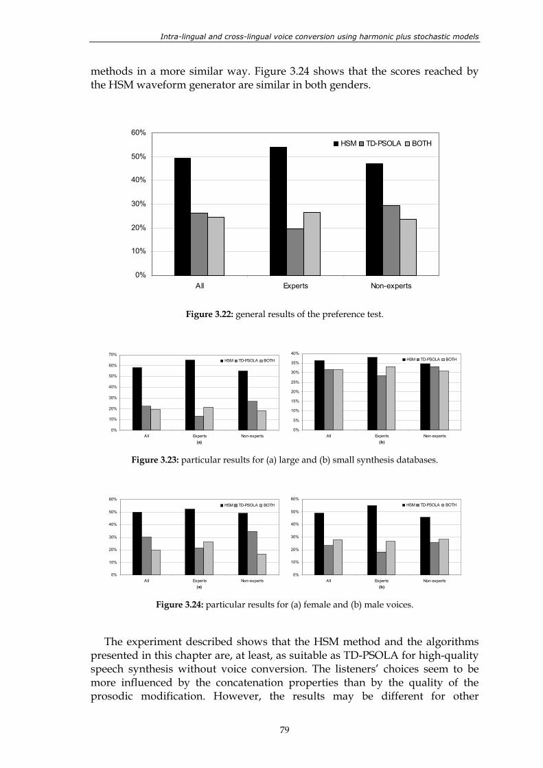
Intra-lingual and cross-lingual voice conversion using harmonic plus stochastic models
79
methods in a more similar way. Figure 3.24 shows that the scores reached by the HSM waveform generator are similar in both genders.
0%
10%
20%
30%
40%
50%
60%
All Experts Non-experts
HSM TD-PSOLA BOTH
Figure 3.22: general results of the preference test.
0%
10%
20%
30%
40%
50%
60%
70%
All Experts Non-experts(a)
HSM TD-PSOLA BOTH
0%
5%
10%
15%
20%
25%
30%
35%
40%
All Experts Non-experts(b)
HSM TD-PSOLA BOTH
Figure 3.23: particular results for (a) large and (b) small synthesis databases.
0%
10%
20%
30%
40%
50%
60%
All Experts Non-experts(a)
HSM TD-PSOLA BOTH
0%
10%
20%
30%
40%
50%
60%
All Experts Non-experts(b)
HSM TD-PSOLA BOTH
Figure 3.24: particular results for (a) female and (b) male voices.
The experiment described shows that the HSM method and the algorithms presented in this chapter are, at least, as suitable as TD-PSOLA for high-quality speech synthesis without voice conversion. The listeners’ choices seem to be more influenced by the concatenation properties than by the quality of the prosodic modification. However, the results may be different for other
Chapter 3. Flexible harmonic plus stochastic speech model
80
configurations of the unit selection procedure that assign a lower weight to the prosodic aspects of the units and a higher weight to the spectral aspects. It must be taken into account that nowadays in a generic speech synthesis application the system tries to minimize the prosodic modifications as possible, whereas in this experiment the strategy was exactly the opposite in order to obtain information about the capability of modifying signals provided by each method. In speech synthesis by concatenation of recorded units without modification, the TD-PSOLA waveform generator can be expected to achieve higher scores because it works directly with the recorded speech samples, but speech synthesis with voice conversion involves important prosodic and spectral modifications, and for this reason the comparison has been carried out under strong modification conditions.
3.5. Conclusions
In this chapter, a new speech model based on a harmonic plus stochastic decomposition has been presented. This model allows manipulating all kind of signal features with a high degree of flexibility, which is desirable for implementing a voice conversion system.
The novelty of the model lies in the algorithms for performing time-scale manipulations, pitch-scale manipulations, and concatenation of units, which are compatible with a non-pitch-synchronous analysis scheme. The reason for preferring a constant analysis frame rate rather than a pitch-synchronous rate is that the analysis procedure is simplified, because the accurate separation of the signal periods is not necessary. In exchange, in order to make artifact-free speech modification possible, the problem of estimating and manipulating the linear-in-frequency phase term of the speech frames without producing artifacts has been faced. In contrast to previous non-pitch-synchronous models based on sinusoidal or hybrid decompositions, it is not necessary to use onset times or pitch-synchronous epochs as a reference. The use of computationally expensive inverse filtering techniques is also avoided. Instead, amplitude and phase envelopes are used as estimators of the vocal tract, assuming a simplified speech production model in which the excitation spectrum has flat magnitude response and linear-in-frequency phase response. A new method for removing the linear phase term from a set of measured harmonics has been also proposed.
In order to validate the suitability of the new model for high-quality speech transformations, a waveform generator using the model and algorithms described here has been implemented and compared to an equivalent TD-PSOLA-based waveform generator. They both have been integrated into the same TTS engine and a preference test has been designed for deciding which of them is better when the prosody of the synthetic speech is forced to be exactly similar to the specifications provided by the TTS system. The results show that listeners have a clear preference for the new system under the conditions of the
Intra-lingual and cross-lingual voice conversion using harmonic plus stochastic models
81
experiment. Since TD-PSOLA is used in standard high-quality synthesis systems, it is concluded that the speech model is also valid for high-quality speech transformation and concatenation. This does not mean that the new model and algorithms are better than TD-PSOLA: probably the quality provided by TD-PSOLA is better when the modification factors are close to 1. However, in voice conversion applications the speech modifications required may be strong.
Now that a very flexible high-quality speech model has been designed, it is time to start converting voices.
Related publications
D. Erro, A. Moreno, “A Pitch-Asynchronous Simple Method for Speech Synthesis by Diphone Concatenation using the Deterministic plus Stochastic Model”, 10th International Conference on Speech and Computer, SPECOM 2005. Patras, Greece, pp. 321-324. October 2005.
D. Erro, A. Moreno, “Efficient Speech Synthesis System using the Deterministic plus Stochastic Model”, 3rd International Conference on Speech Prosody 2006. Dresden, Germany. May 2006.
D. Erro, A. Moreno, “Flexible Harmonic/Stochastic Speech Synthesis”, 6th ISCA Workshop on Speech Synthesis. Bonn, Germany. August 2007.

Chapter 3. Flexible harmonic plus stochastic speech model
82
83
4. New techniques for high-quality voice conversion
The analysis of the state of the art of voice conversion technologies carried out in chapter 2 shows that converting voices implies certain quality degradation in the synthetic speech. It can be observed that, regardless of the spectral manipulation method adopted by the voice conversion system, the similarity between the converted voices and the target voices is highly correlated to the quality loss with respect to the original signal, so it can be stated that in general, obtaining a higher converted-to-target similarity implies also obtaining higher quality degradation. There are two main reasons for this:
All kinds of artificial signal manipulations (including the prosodic modification of natural speech) entail degradation. The more conversion accuracy is required, the higher degree of spectral manipulation is necessary, and therefore the more noticeable degradation is produced.
A higher acoustic quality allows the listeners perceiving the differences between the converted and target speakers more clearly. For instance, one can easily imitate someone’s voice by telephone, because the low signal-to-noise ratio muffles the differences between voices and makes it more difficult for the listener to distinguish them. Also, it is known that, for the same reason, higher perceptual quality scores are obtained by a TTS system when its output is combined with a sweet musical melody.
According to the objectives of this thesis, it is intended to research into voice conversion methods (see figure 4.1) capable of transforming the short-time spectrum of signals without significant quality loss. Since there is a trade-off between the quality and the conversion degree, in this chapter the objective is to design a voice conversion method that provides state-of-the-art performance in terms of converted-to-target similarity and reaches higher quality scores. Priority will be given to the quality of the converted speech, because the quality scores achieved so far by state-of-the-art voice conversion systems, particularly the systems that have a satisfactory performance in terms of converted-to-target similarity, are still low compared to those that could be suitable for real-life applications.
This chapter is structured as follows.
In section 4.1, the most relevant contributions to voice conversion technologies are mentioned and briefly described.
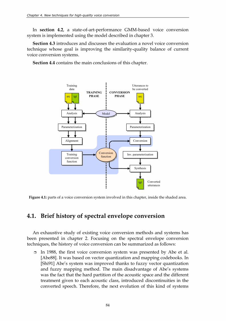
Chapter 4. New techniques for high-quality voice conversion
84
In section 4.2, a state-of-art-performance GMM-based voice conversion system is implemented using the model described in chapter 3.
Section 4.3 introduces and discusses the evaluation a novel voice conversion technique whose goal is improving the similarity-quality balance of current voice conversion systems.
Section 4.4 contains the main conclusions of this chapter.
Figure 4.1: parts of a voice conversion system involved in this chapter, inside the shaded area.
4.1. Brief history of spectral envelope conversion
An exhaustive study of existing voice conversion methods and systems has been presented in chapter 2. Focusing on the spectral envelope conversion techniques, the history of voice conversion can be summarized as follows:
In 1988, the first voice conversion system was presented by Abe et al. [Abe88]. It was based on vector quantization and mapping codebooks. In [Shi91] Abe’s system was improved thanks to fuzzy vector quantization and fuzzy mapping method. The main disadvantage of Abe’s systems was the fact that the hard partition of the acoustic space and the different treatment given to each acoustic class, introduced discontinuities in the converted speech. Therefore, the next evolution of this kind of systems
Converted utterances
Analysis
Parameterization
Alignment
Training conversion
function
Analysis
Parameterization
Conversion
Synthesis
tgt
Inv. parameterization
TRAINING PHASE
CONVERSION PHASE src tgt
Training data
Utterances to be converted
src
Model
Conversion function
Intra-lingual and cross-lingual voice conversion using harmonic plus stochastic models
85
consisted of changing the way of processing each acoustic class: in [Val92] the vectors inside each class were normalized and multiplied by a different transformation matrix; in [Miz94] each class was assigned a set of transformation rules to be applied to the formant parameters; in [Ars99, Tur06] a filter was calculated for each input vector by weighted combination of the codebook vectors, using a fuzzy classification to calculate the weights; in [Sal06], for a given source vector sequence the best sequence of codewords of the target speaker was found by dynamic programming.
In 1992, Valbret et al. proposed to use the dynamic frequency warping technique for voice conversion [Val92]. Other frequency-warping-based techniques were presented in [Sün03a, Ren04, Shu06]. All these systems had one thing in common: they provided high-quality converted speech, but the similarity scores between converted and target voices were not satisfactory because the formants were just moved to new frequencies without altering the spectral shape.
In 1994, it was proposed to combine different recorded voices to obtain the target voice through speaker interpolation [Iwa94, Iwa95]. Although this technique was not very successful, the same underlying idea was used some years later to build multi-speaker systems based on different transformation techniques [Tam01, Lat06, Tod06].
In 1995, artificial neural networks were used for voice conversion [Nar95], but the immediate appearance of GMM-based systems put this method aside [Bau96].
In 1996, Stylianou used gaussian mixture models for partitioning the acoustic space into overlapping classes, and he defined a continuous probabilistic transformation function for the acoustic vectors [Sty96, Sty98]. This method was improved by Kain in 2001 [Kai01]. Thus, the discontinuities that appeared in previous codebook-based methods were completely avoided, so high similarity scores and satisfactory quality scores were obtained. The main problem turned to be the over-smoothing introduced by the new transformation method, so some solutions were proposed in [Tod01, Che03, Tod05, Ye06], but in essence the GMM-based approach remained similar to Kain’s.
Approximately at the same time, in 1996, speech synthesis by HMMs was born [Mas96]. In order to integrate voice conversion into this kind of synthesis systems [Mas97], adaptation procedures were used to modify the models of a given source speaker to fit the acoustic space defined by the observed vectors of the target speakers. The modified HMMs were used to synthesize utterances with the target voice. Some other HMM-based methods were [Tam98, Mor03, Dux04].
In 2001, when the vocal tract conversion scores reached satisfactory levels thanks to GMM-based systems, the research was focused on the transformation of residuals. Different strategies were adopted: residual
Chapter 4. New techniques for high-quality voice conversion
86
codebooks [Ars99, Kai01, Ye06], residual selection [Ye04a], selection and smoothing [Sün05], frequency-warping of residuals [Sün06a], etc. It was also proved that it was a better idea to predict residuals from converted vocal tracts than to convert the residuals of the source speaker [Dux06a].
It can be affirmed that GMM-based systems are still the most popular at present. Moreover, the fact that the research has been focused on residuals during the last years indicates that GMM-based voice conversion systems have achieved a satisfactory performance at converting the vocal tract of the involved speakers.
4.2. Baseline system based on GMMs
The objective here is to implement a state-of-the-art voice conversion system to be used as a starting point for introducing improvements. This means choosing and combining the most adequate methods for signal analysis/reconstruction, alignment of source and target features, envelope parameterization and transformation, etc. In practice, the choice of the spectral envelope transformation technique is the most important one, because it directly influences the quality and similarity scores achieved by the whole system. According to the bibliographic analysis carried out in chapter 2 and summarized in the previous section, GMM-based statistical transformation method is the most reasonable choice.
4.2.1. Fundamentals of GMM-based voice conversion
Gaussian mixture models are probability density functions built as a weighted sum of m gaussian components:
( ) ( )∑=
=m
iiii Np
1, ; Σµxx α (4.1)
Each of the m Gaussian components are themselves gaussian probability density functions for p-dimensional vectors, described as follows:
( ) ( ) ( ) ( )iiT
ieN ip
iiµxΣµxΣΣµx −−−−− −
=1
212/12/2, ; π (4.2)
where µi denotes the p-dimensional mean vector of each component and Σi is its p×p covariance matrix. For p(x) to be a probability density function, the weights of the combination αi have to be positive numbers verifying the following condition:
11
=∑ =
m
i iα (4.3)
Intra-lingual and cross-lingual voice conversion using harmonic plus stochastic models
87
The GMM is completely defined by the weights, mean vectors and covariance matrices of its individual components αi, µi, Σi. Such model can be used to obtain a soft partition of the vector space, where the probability of a vector x to belong to the ith class (or gaussian component), pi(x), can be expressed as
( ) ( )( )∑ =
= m
q qqq
iiii
NNp
1, ;
, ;Σµx
Σµxxα
α (4.4)
Given a set of N vectors X=xk and a certain GMM, the likelihood of the whole set with respect to the model is given by the product of all the individual contributions:
( ) ( )∏=
=N
kkpXP
1x (4.5)
The way of estimating the parameters of the GMM that best fits a given set of vectors X consists of finding the model for which the global likelihood P(X) is maximal. This problem, which is equivalent to maximizing the log-likelihood function log P(X), does not have a straightforward analytical solution, but an increasingly good approximation can be obtained by the iterative Expectation-Maximization (EM) algorithm. Given an initial model for X, αi(r), µi(r), Σi(r), the EM algorithm calculates a new model αi(r+1), µi(r+1), Σi(r+1) with higher associated log-likelihood by maximizing an auxiliary function. The algorithm consists of the following steps:
1. An initial estimate of the GMM parameters αi(0), µi(0), Σi(0) is calculated. This can be done by grouping the vectors of the set X into m clusters from which the mean vectors and covariance matrices are obtained. The weights of the gaussian components can be initialized by dividing the number of vectors inside each cluster by the total number of vectors, N.
2. E-step: given the current estimate of the model parameters αi(r), µi(r), Σi(r), the a posteriori classification probabilities pi(xk)(r) are calculated for all the vectors in X by means of equation (4.4).
3. M-step: new model parameters αi(r+1), µi(r+1), Σi(r+1) are calculated from the probabilities pi(xk)(r) as follows:
( )
( )( )
( ) ( )( )( )∑
∑∑∑
∑
=
=++
+
=
=+
=
+
−−=
=
=
N
kr
ki
N
k
Trik
rik
rkir
i
N
kr
ki
N
k kr
kiri
N
k
rki
ri
p
p
p
p
pN
1)(
1)1()1()(
)1(
1)(
1)(
)1(
1
)()1( 1
x
µxµxxΣ
x
xxµ
xα
(4.6)
(4.7)
(4.8)
4. The EM steps (2 and 3) are iterated until the log-likelihood improvement is not significant anymore.
Chapter 4. New techniques for high-quality voice conversion
88
The EM algorithm converges to a local maximum of the log-likelihood function, so the convergence is conditioned by the initialization. For this reason, it is adequate to use hard clustering of the vector space for estimating the initial model, instead of using other alternatives with higher randomness. It has been noticed that the numerical problems that appear when inverting the covariance matrices are important. In order to avoid them, a small perturbation is added to the successive covariance estimates.
In voice conversion systems based on GMMs, each vector xk contains an acoustic representation of the speaker’s vocal tract or spectral envelope. Cepstral coefficients and line spectral frequencies derived from all-pole filters are the most usual acoustic parameterizations used for translating the speech frames into constant-length acoustic vectors. The whole acoustic space of a given speaker can be represented by the GMM that better fits the set of acoustic vectors extracted from a training database. In this situation, different methods have been proposed for transforming source acoustic vectors into target vectors.
The first GMM-based transformation method was published by Stylianou [Sty96]. Given N source acoustic vectors X=xk and their corresponding N target vectors Y=yk obtained from a parallel training corpus, a GMM αix, µix, Σixx is estimated from X and the a posteriori probabilities pix(xk) are calculated. Stylianou proposes to apply the following transformation function:
( ) ( ) ( )[ ]∑=
−−+=
m
i
xi
xxiii
xipF
1
1 µxΣΓνxx (4.9)
where the p-dimensional vectors νi and the p×p-dimensional matrices Γi are determined by minimizing through the whole dataset the transformation error given by
( )( )2xy F−Ε=ε (4.10)
This is equivalent to defining an optimal linear transformation for each of the gaussian components and building the global transformation by combining the m contributions.
The method proposed by Kain some years later [Kai01] consists of building a set of concatenated vectors Z=zk, zk=[xkT ykT]T, and modeling the space of Z by a GMM αi, µiz, Σizz. The mean vectors and covariance matrices of this model verify the following relationships:
=
= yy
iyxi
xyi
xxizz
iyi
xiz
i ΣΣΣΣ
Σµµ
µ , (4.11)
Therefore, implicit information about the individual acoustic spaces of X and Y, and also about the cross-covariance matrices, is obtained. Thus, the transformation function can be derived directly from the trained model, as
( ) ( ) ( ) ( ) ( )[ ]∑∫=
−−+=⋅=Ε=
m
i
xi
xxi
yxi
yi
xipdpF
1
1 µxΣΣµxyxyyxyx (4.12)
Intra-lingual and cross-lingual voice conversion using harmonic plus stochastic models
89
As it has been explained in chapter 2, some other types of GMM-based transformation functions, designed to face the over-smoothing problem that appears in standard GMM-based systems, have been proposed [Che03, Tod05]. Anyway, in spite of the over-smoothing problem, this type of systems generally performs better than others.
4.2.2. Description of the system
This section describes how the different tasks of the voice conversion process are implemented in the baseline system. Although the techniques applied here do not contain relevant novelties with respect to the state of the art, the way of implementing a GMM-based voice conversion system using the non-pitch-synchronous Harmonic plus Stochastic model described in chapter 3 has some particularities that make it different from the others. In the next sub-sections, the implementation of the baseline system is detailed according to the structure of a generic voice conversion system, shown in figure 4.1.
Speech model
The HSM represents the speech signal frames by the local pitch frequency, the amplitudes and phases of the harmonics below 5 KHz and the LPC coefficients of the stochastic component. All these parameters should be successfully transformed by the voice conversion system. The speech model has been described extensively in chapter 3, so no more details are given here.
Parameterization
The task of converting voices directly from the HSM parameters (amplitudes, frequencies, phases and stochastic filters) is extremely complicated. The strategy usually followed in this situation consists of decomposing the whole voice conversion problem into different sub-problems that can be solved independently:
Pitch conversion. Parameterization of the f0 information is not necessary, since only its mean level is to be converted.
Harmonic conversion related to the amplitudes and phases. In previous voice conversion studies it was stated that the influence of the harmonic component in the listeners’ perception is much more decisive than that of unvoiced sounds [Ye04a]. However, the amplitudes and phases do not provide a suitable parameterization of the harmonic spectral envelope in terms of voice conversion for several reasons: (i) the number of harmonics is variable, whereas GMM transformations are applied to constant-length vectors; (ii) the number of harmonics is, in general, high, what makes the conversion process more complicated; (iii) the sinusoid
Chapter 4. New techniques for high-quality voice conversion
90
parameters do not have good interpolation properties. Therefore, an adequate harmonic parameterization is necessary.
Stochastic conversion, related to the LPC stochastic filters. In this case, the LPC coefficients used for modeling the signal aperiodic component constitute a valid parameterization by themselves.
Therefore, the task is narrowed to finding the most appropriate parameterization for the harmonic component. In current voice conversion systems, two main types of coefficients are used for this purpose:
Cepstral coefficients (CC): they are defined as such coefficients ci that the log-amplitude spectrum can be modelled as
( ) ( )∑=
+≈p
isi fifccfX
10 2cos2log π (4.13)
Given a set of harmonics, the optimum sequence of cepstral coefficients can be obtained through a least squares optimization [Sty96]. In general, c0 is discarded for voice conversion because it only represents the energy of the spectrum instead of its shape.
Line spectral frequencies (LSFs): given a pth order all-pole representation of the spectrum, 1/A(z), the LSF coefficients are the roots of the following (p+1)th order polynomials:
( ) ( ) ( ) ( )( ) ( ) ( ) ( )11
11
−+−
−+−
−=
+=
zAzzAzQzAzzAzP
p
p
(4.14)
P is a palindromic polynomial and Q an anti-palindromic polynomial. P(z) and Q(z) have all their roots on the unit circle, so they can be completely characterized by the frequencies where the roots are located. As the roots of P and Q occur in symmetrical pairs at positive and negative frequencies (except for two roots that appear always at 0 and π), only p/2 frequencies need to be stored for each polynomial, so the output of the LSF search has dimension p. Given a certain set of LSFs, their associated A(z) is obtained easily as 0.5·(P(z)+Q(z)). When the roots of P(z) and Q(z) are interleaved, the stability of the filter 1/A(z) is ensured if and only if the roots are monotonously increasing. Moreover, the closer two LSFs are, the more resonant the filter is at the corresponding frequency. In voice conversion applications, LSFs are preferred rather than other types of parameterization for several reasons:
i) All-pole filters are a good representation of the formant structure.
ii) They have very good interpolation properties.
iii) If one of the coefficients is erroneously converted, this affects only a small portion of the spectrum.
In the context of this thesis, LSF coefficients have also some extra advantages:
Intra-lingual and cross-lingual voice conversion using harmonic plus stochastic models
91
iv) The cepstral coefficients associated to a certain LSF vector can be calculated in an efficient way from the coefficients of A(z), if necessary (see expression (4.46)). In other words, LSFs contain an implicit CC parameterization. This property will be exploited in chapters 4 and 5.
v) When converted LSF vectors are translated back into all-pole filters, the minimum phase response of the filters is valid for estimating the phase envelope of the target speaker.
vi) Since the stochastic component is represented by LPC coefficients, the same kind of parameterization would be used for the harmonic component and for the stochastic component. This is advantageous for prediction of one component from the other.
It can be concluded that LSFs are the best option in this case. A particularized frequency-domain implementation of the LPC technique [Mak75] can be applied to obtain the optimal all-pole representation of a given set of harmonics. It is well known that the coefficients of an LPC filter of the form
( ) pp zazazA −− +++
=K1
1111 (4.15)
can be calculated by solving the following system:
−
−−
=
⋅
−−
−
−
pppp
p
p
R
RR
a
aa
RRR
RRRRRR
MM
L
MOMM
L
L
2
1
2
1
021
201
110
(4.16)
The sequence [R0 … Rp] corresponds to the first p+1 values of the autocorrelation sequence of the input signal x[n]. The system matrix is a Toeplitz matrix, so it can be inverted efficiently by means of the Levinson-Durbin recursion [Lev47, Dur60]. In the case of harmonic signals given by the amplitudes, frequencies and phases of the sinusoids, the values of Rn are more easily calculated using the inverse Fourier transform of the power spectrum:
( ) ( ) ( )∑∑∫ =+=∝ −
−l
lll
njwnjwl
jwnn nwAeeAdwewXR ll cos2
212
412π
π (4.17)
where the ½ factor can be omitted. Although this procedure is simple and efficient, a more precise all-pole representation of a given set of spectral points is obtained by minimizing the Itakura-Saito (I-S) error, given by the following expression:
( )( )
( )( )∑
=−
−−=
L
l l
l
l
lSI wP
wPwPwP
L 1** 1ln1ε (4.18)
where L is the number of harmonics, P represents the power spectrum of the signal at the specified frequencies (which is equivalent to the squared amplitude) and P* is obtained from the estimated all-pole filter. The Discrete
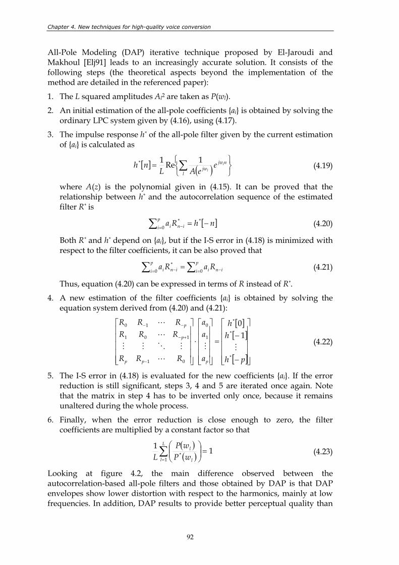
Chapter 4. New techniques for high-quality voice conversion
92
All-Pole Modeling (DAP) iterative technique proposed by El-Jaroudi and Makhoul [Elj91] leads to an increasingly accurate solution. It consists of the following steps (the theoretical aspects beyond the implementation of the method are detailed in the referenced paper):
1. The L squared amplitudes Al2 are taken as P(wl).
2. An initial estimation of the all-pole coefficients ai is obtained by solving the ordinary LPC system given by (4.16), using (4.17).
3. The impulse response h* of the all-pole filter given by the current estimation of ai is calculated as
[ ] ( )
= ∑l
njwjw
l
le
eALnh 1Re1* (4.19)
where A(z) is the polynomial given in (4.15). It can be proved that the relationship between h* and the autocorrelation sequence of the estimated filter R* is
[ ]nhRap
i ini −=∑ = −*
0* (4.20)
Both R* and h* depend on ai, but if the I-S error in (4.18) is minimized with respect to the filter coefficients, it can be also proved that
∑∑ = −= − =p
i inip
i ini RaRa00
* (4.21)
Thus, equation (4.20) can be expressed in terms of R instead of R*.
4. A new estimation of the filter coefficients ai is obtained by solving the equation system derived from (4.20) and (4.21):
[ ][ ]
[ ]
−
−=
⋅
−
+−
−−
ph
hh
a
aa
RRR
RRRRRR
ppp
p
p
*
*
*
1
0
01
101
10
10
MM
L
MOMM
L
L
(4.22)
5. The I-S error in (4.18) is evaluated for the new coefficients ai. If the error reduction is still significant, steps 3, 4 and 5 are iterated once again. Note that the matrix in step 4 has to be inverted only once, because it remains unaltered during the whole process.
6. Finally, when the error reduction is close enough to zero, the filter coefficients are multiplied by a constant factor so that
( )( )∑
=
=
L
l l
l
wPwP
L 1* 11 (4.23)
Looking at figure 4.2, the main difference observed between the autocorrelation-based all-pole filters and those obtained by DAP is that DAP envelopes show lower distortion with respect to the harmonics, mainly at low frequencies. In addition, DAP results to provide better perceptual quality than
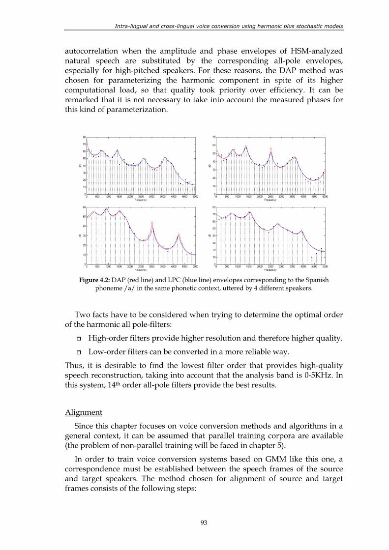
Intra-lingual and cross-lingual voice conversion using harmonic plus stochastic models
93
autocorrelation when the amplitude and phase envelopes of HSM-analyzed natural speech are substituted by the corresponding all-pole envelopes, especially for high-pitched speakers. For these reasons, the DAP method was chosen for parameterizing the harmonic component in spite of its higher computational load, so that quality took priority over efficiency. It can be remarked that it is not necessary to take into account the measured phases for this kind of parameterization.
Figure 4.2: DAP (red line) and LPC (blue line) envelopes corresponding to the Spanish
phoneme /a/ in the same phonetic context, uttered by 4 different speakers.
Two facts have to be considered when trying to determine the optimal order of the harmonic all pole-filters:
High-order filters provide higher resolution and therefore higher quality.
Low-order filters can be converted in a more reliable way.
Thus, it is desirable to find the lowest filter order that provides high-quality speech reconstruction, taking into account that the analysis band is 0-5KHz. In this system, 14th order all-pole filters provide the best results.
Alignment
Since this chapter focuses on voice conversion methods and algorithms in a general context, it can be assumed that parallel training corpora are available (the problem of non-parallel training will be faced in chapter 5).
In order to train voice conversion systems based on GMM like this one, a correspondence must be established between the speech frames of the source and target speakers. The method chosen for alignment of source and target frames consists of the following steps:
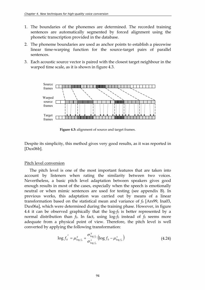
Chapter 4. New techniques for high-quality voice conversion
94
1. The boundaries of the phonemes are determined. The recorded training sentences are automatically segmented by forced alignment using the phonetic transcription provided in the database.
2. The phoneme boundaries are used as anchor points to establish a piecewise linear time-warping function for the source-target pairs of parallel sentences.
3. Each acoustic source vector is paired with the closest target neighbour in the warped time scale, as it is shown in figure 4.3.
Figure 4.3: alignment of source and target frames.
Despite its simplicity, this method gives very good results, as it was reported in [Dux06b].
Pitch level conversion
The pitch level is one of the most important features that are taken into account by listeners when rating the similarity between two voices. Nevertheless, a basic pitch level adaptation between speakers gives good enough results in most of the cases, especially when the speech is emotionally neutral or when mimic sentences are used for testing (see appendix B). In previous works, this adaptation was carried out by means of a linear transformation based on the statistical mean and variance of f0 [Ars99, Ina03, Dux06a], which were determined during the training phase. However, in figure 4.4 it can be observed graphically that the log-f0 is better represented by a normal distribution than f0. In fact, using log-f0 instead of f0 seems more adequate from a physical point of view. Therefore, the pitch level is well converted by applying the following transformation:
( )xfx
f
yfy
f ff0
0
0
0 log0log
loglog0 loglog µ
σσ
µ −+=′ (4.24)
Source frames
Warped source frames
Target frames
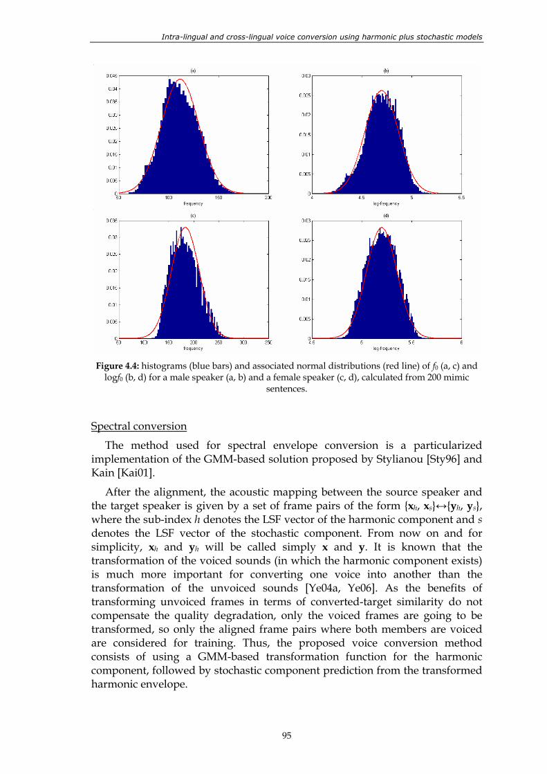
Intra-lingual and cross-lingual voice conversion using harmonic plus stochastic models
95
Figure 4.4: histograms (blue bars) and associated normal distributions (red line) of f0 (a, c) and
logf0 (b, d) for a male speaker (a, b) and a female speaker (c, d), calculated from 200 mimic sentences.
Spectral conversion
The method used for spectral envelope conversion is a particularized implementation of the GMM-based solution proposed by Stylianou [Sty96] and Kain [Kai01].
After the alignment, the acoustic mapping between the source speaker and the target speaker is given by a set of frame pairs of the form xh, xs↔yh, ys, where the sub-index h denotes the LSF vector of the harmonic component and s denotes the LSF vector of the stochastic component. From now on and for simplicity, xh and yh will be called simply x and y. It is known that the transformation of the voiced sounds (in which the harmonic component exists) is much more important for converting one voice into another than the transformation of the unvoiced sounds [Ye04a, Ye06]. As the benefits of transforming unvoiced frames in terms of converted-target similarity do not compensate the quality degradation, only the voiced frames are going to be transformed, so only the aligned frame pairs where both members are voiced are considered for training. Thus, the proposed voice conversion method consists of using a GMM-based transformation function for the harmonic component, followed by stochastic component prediction from the transformed harmonic envelope.
Chapter 4. New techniques for high-quality voice conversion
96
The harmonic envelope transformation function is similar to that proposed by Kain (expression (4.12)). During the training phase, paired p-dimensional LSF vectors x and y are concatenated together to form 2p-dimensional vectors z=[xT yT]T. A joint GMM estimated from z provides complete information about the individual acoustic space of each speaker, given by the weights, mean vectors and covariance matrices of the m Gaussian components, αi, µix, Σixx and αi, µiy, Σiyy, but also about the cross-covariance matrices Σixy and Σiyx. During the conversion phase, given a source vector x, the corresponding converted LSF vector F(x) is obtained by applying equation (4.12). The inverse-parameterization process is carried out by resampling the converted all-pole envelope H(k)(z) at the positions of the new harmonics (which are multiples of the converted f0). Thus, the converted amplitudes are obtained by multiplying the module of the spectral samples by a certain positive factor η so that the energy of the converted harmonics equals the energy of the source harmonics.
( )0)()( jlwkkl eHA η= (4.25)
The minimum phase response of the converted all-pole filter can be considered to be a valid estimation of the phase envelope. Although it may not coincide with the real phase envelope, due to its physical meaning, it provides phase values that are correlated with the converted amplitudes at every frame. The correlation between magnitude and phase is very important for obtaining realistic speech waveforms. Moreover, the quality loss produced by the minimum-phase approach is insignificant compared to that produced by the spectral conversion process. The linear-in-frequency phase term can also be artificially generated assuming that the pitch varies linearly from one voiced frame to the next, using the function ψ defined in chapter 3 (expression 3.34). Thus, the converted phases φl(k)are given by the following recursion:
( ) ( ) ( )NwwNww
leHkkkkkkk
kjlwkkl
)(0
)1(02
1)1()(0
)1(0
)1()(
)()()(
,,arg 0
++=+=
+=−−−− αψαα
αϕ (4.26)
The linear phase term α can be considered to be zero at the beginning of each voiced region. Since the phase information is extracted from the converted filter, the phases of the source frame do not take part in the spectral envelope conversion. Therefore, it is not necessary to apply pitch modification techniques for the pitch level adaptation between speakers. Instead, the converted pitch is calculated using equation (4.24) and the new amplitudes and phases are generated by equations (4.25) and (4.26).
Under the assumption that the stochastic component is highly correlated with the harmonic component in voiced frames, a stochastic envelope prediction function can be learnt using the training speech frames of the target speaker. Once the transformation function for the harmonic component is trained, all the harmonic-stochastic vector pairs of the form y, ys and the target speaker’s acoustic model αi, µiy, Σiyy can be used for calculating the m vectors νi and matrices Гi that minimize the error of the following prediction function:
Intra-lingual and cross-lingual voice conversion using harmonic plus stochastic models
97
( ) ( )[ ]∑=
−−+=
m
i
yi
yyiii
yis p
1
1 µyΣΓνyy (4.27)
A similar function was used by Stylianou for transforming the harmonic component [Sty96]. In this case it is used for stochastic prediction, instead. The problem can be solved by a least squares optimization:
[ ] sYRV
DP =
⋅ (4.28)
where
( ) ( )
( ) ( )
=
=
=
=
NymN
y
ym
y
Tm
T
Tm
T
TsN
Ts
s
pp
pp
yy
yyP
Γ
ΓR
ν
νV
y
yY
L
MOM
L
MMM
1
111111
, , ,
( )( ) ( ) ( )( ) ( )
( )( ) ( ) ( )( ) ( )
−−
−−=
−−
−−
Tyym
TymNN
ym
TyyTyNN
y
Tyym
Tym
ym
TyyTyy
pp
pp
11111
111
111111
ΣµyyΣµyy
ΣµyyΣµyyD
L
MOM
L
(4.29)
The optimal solution is
[ ]( ) sopt
YDPRV
⋅=
pinv (4.30)
where pinv(·) denotes the pseudo-inverse matrix. During the conversion phase, the prediction function is applied to the converted harmonic vector F(x).
4.2.3. Tuning of the system
Although objective measures are not suitable for determining whether a voice conversion system is good or not, they can be used to find the most appropriate dimensioning of the system. For this purpose, an experiment was carried out under the following conditions:
Four different voices of two male (m1, m2) and two female speakers (f1, f2) were used. Thus, twelve conversion directions were possible. The sentences were the same for all the speakers, so a parallel corpus could be built for each conversion direction.
The parallel training corpus was split into two parts: the first one was used for training, and the second one, composed by 10 parallel sentences for each conversion direction, was used for testing. The number of training sentences, whose average duration was 4 seconds, is one of the variables of this experiment. The other variable is the order (number of gaussian components) of the GMM used for transforming parameter vectors.
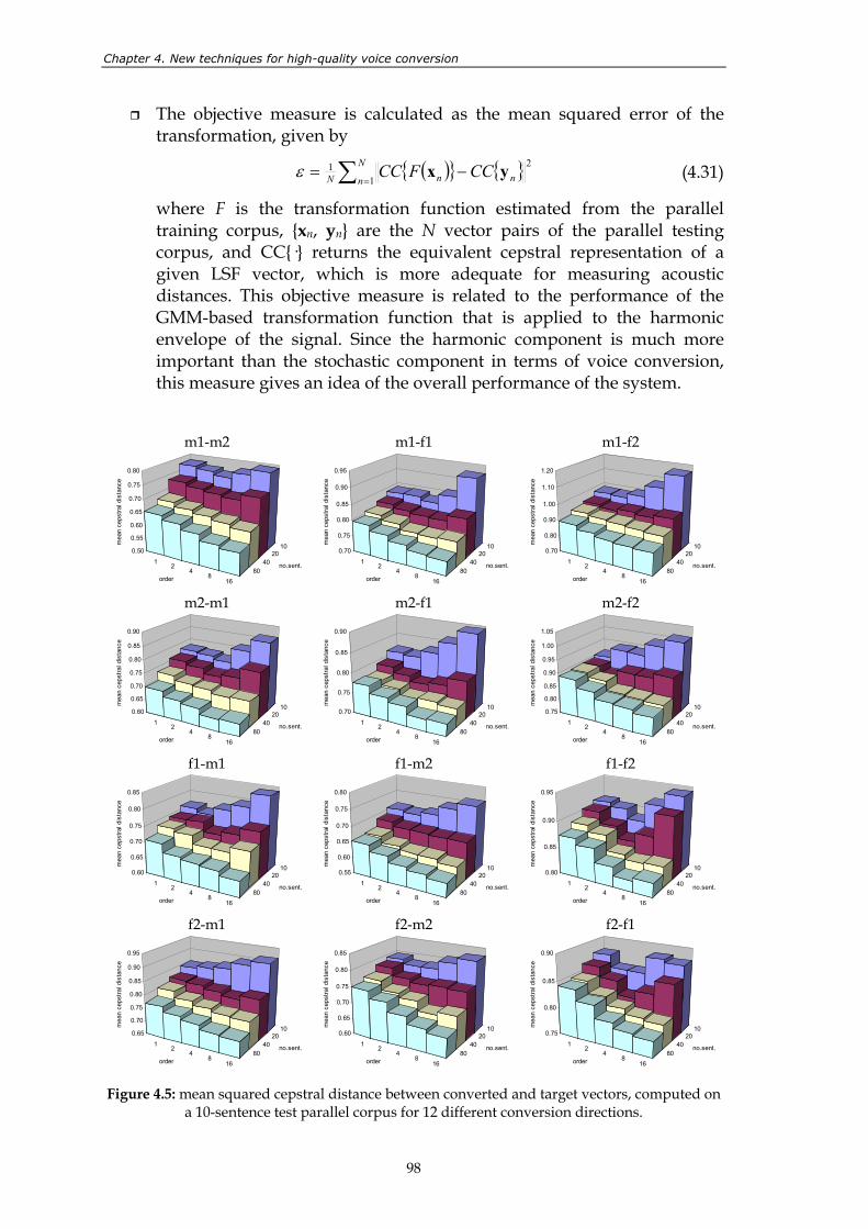
Chapter 4. New techniques for high-quality voice conversion
98
The objective measure is calculated as the mean squared error of the transformation, given by
( ) ∑ =−=
N
n nnN CCFCC1
21 yxε (4.31)
where F is the transformation function estimated from the parallel training corpus, xn, yn are the N vector pairs of the parallel testing corpus, and CC· returns the equivalent cepstral representation of a given LSF vector, which is more adequate for measuring acoustic distances. This objective measure is related to the performance of the GMM-based transformation function that is applied to the harmonic envelope of the signal. Since the harmonic component is much more important than the stochastic component in terms of voice conversion, this measure gives an idea of the overall performance of the system.
m1-m2
12
48
1680
4020
100.50
0.55
0.60
0.65
0.70
0.75
0.80
mea
n ce
pstra
l dis
tanc
e
order
no.sent.
m1-f1
12
48
1680
4020
100.70
0.75
0.80
0.85
0.90
0.95
mea
n ce
pstra
l dis
tanc
e
order
no.sent.
m1-f2
12
48
1680
4020
100.70
0.80
0.90
1.00
1.10
1.20
mea
n ce
pstra
l dis
tanc
e
order
no.sent.
m2-m1
12
48
1680
4020
100.60
0.65
0.70
0.75
0.80
0.85
0.90
mea
n ce
pstra
l dis
tanc
e
order
no.sent.
m2-f1
12
48
1680
4020
100.70
0.75
0.80
0.85
0.90
mea
n ce
pstra
l dis
tanc
e
order
no.sent.
m2-f2
12
48
1680
4020
100.75
0.80
0.85
0.90
0.95
1.00
1.05
mea
n ce
pstra
l dis
tanc
e
order
no.sent.
f1-m1
12
48
1680
4020
100.60
0.65
0.70
0.75
0.80
0.85
mea
n ce
pstra
l dis
tanc
e
order
no.sent.
f1-m2
12
48
1680
4020
100.55
0.60
0.65
0.70
0.75
0.80
mea
n ce
pstra
l dis
tanc
e
order
no.sent.
f1-f2
12
48
1680
4020
100.80
0.85
0.90
0.95
mea
n ce
pstra
l dis
tanc
e
order
no.sent.
f2-m1
12
48
1680
4020
100.65
0.70
0.75
0.80
0.85
0.90
0.95
mea
n ce
pstra
l dis
tanc
e
order
no.sent.
f2-m2
12
48
1680
4020
100.60
0.65
0.70
0.75
0.80
0.85
mea
n ce
pstra
l dis
tanc
e
order
no.sent.
f2-f1
12
48
1680
4020
100.75
0.80
0.85
0.90
mea
n ce
pstra
l dis
tanc
e
order
no.sent.
Figure 4.5: mean squared cepstral distance between converted and target vectors, computed on
a 10-sentence test parallel corpus for 12 different conversion directions.
Intra-lingual and cross-lingual voice conversion using harmonic plus stochastic models
99
Figure 4.5 displays the mean squared transformation error obtained for all of the conversion directions, using a varying number of training sentences (from 10 to 80) and different GMM orders (from 1 to 16). Low error values indicate that the conversion accuracy is good. It has to be taken into account that the error values shown in the figure correspond to the dimensions and the specific implementation of the described system. Using diagonal covariance matrices or increasing the dimension of the parameter vectors would result in different error values. Looking at the surfaces defined by the error measure, several phenomena can be observed. In general, the distortion is diminished by increasing the GMM order and the number of training sentences, but:
Increasing the number of gaussian components while keeping the number of sentences low is harmful for the system. When a high-order GMM is fitted to very few data, the model learns the specific vectors seen during the training phase rather than the whole acoustic space. This phenomenon is called over-fitting.
Increasing the number of training sentences has a positive effect on the distortion, but the improvements are significant only if the order of the model is also increased according to the amount of training data. The effect of over-smoothing occurs when a low-order model is fitted to a large amount of data.
The surfaces obtained for different source and target speakers have also different behaviour, so it is difficult to determine the optimal GMM order for a given number of training sentences without considering speaker-dependent factors. Dimensioning is one of the main problems of GMM-based voice conversion, which can be solved by reserving some of the parallel training sentences for comparing a-posteriori several transformation functions with different orders, and choosing the one that provides minimal distortion.
Increasing the order of the trained models from 8 to 16 leads to obtaining slightly more accurate transformation functions if the number of training sentences is high enough, but it also implies a noticeable increment of the computational load. Informal tests indicate that such small improvements in the objective distortion measure are hardly perceived by the listeners, so in practice the benefit obtained from 16th order GMMs does not compensate the time required for their estimation.
It can be concluded that in a standard voice conversion task, where only few minutes of audio are available for training, around 4 or 8 gaussian components should be used.
Chapter 4. New techniques for high-quality voice conversion
100
4.2.4. Subjective evaluation
Within the framework of the European integrated project TC-STAR, public competitive evaluations were organized annually in order to encourage significant advances in all the technologies involved in speech-to-speech translation. Independent evaluations were carried out for automatic speech recognition, spoken language translation and text-to-speech synthesis plus voice conversion, for three different languages: European English, European Spanish, and Mandarin Chinese.
During the second Evaluation Campaign of the TC-STAR project [Mos06], the first version of the system described above was subjectively evaluated by listeners, under the following conditions:
20 listeners were asked to listen to several sentence pairs in which one of the sentences had been converted by the system and the other one was a recorded utterance of the target speaker. The evaluators were asked to identify if both samples came from the same person or not, using a 5-point scale (5=”definitely identical”, 4=”probably identical”, 3=”not sure”, 2=”probably different”, 1=”definitely different”). The scores were assigned without paying attention to the quality or the recording conditions. For the same pair of samples, in the next step, the listeners were asked to rate also the quality of the converted sentences from 1=”bad” to 5=”excellent”.
4 different voices were used in this perceptual test: 2 male voices (m1, m2) and 2 female voices (f1, f2). One male and one female were chosen as source speakers and the two remaining voices were chosen as target speakers, and 4 different conversion directions were considered: male to male (m1-m2), male to female (m1-f2), female to male (f1-m2) and female to female (f1-f2). For a given conversion direction, an average score was calculated from the listeners’ individual scores.
All the speakers involved were bilingual: for each speaker, around 150 sentences in Spanish and 150 in English were available for training. The average duration of the sentences was 3 or 4 seconds. 10 sentences unseen during the training process were used for the perceptual test. The sentences uttered by all the speakers were the same, so that a parallel corpus could be created. All of them were mimic sentences, so there were no significant prosodic differences between speakers.
The characteristics of the evaluated systems (for privacy, they are given fictitious names here) were the following:
Proposed system: the one described above. The system was configured to use 8th order GMMs and 14-dimensional LSF vectors. Since the system was not yet optimized for this evaluation, the stochastic component was not modified at all (in further versions, the stochastic prediction procedure was incorporated to the system). With regard to the
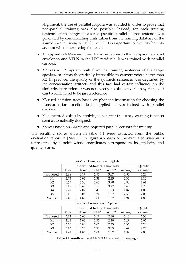
Intra-lingual and cross-lingual voice conversion using harmonic plus stochastic models
101
alignment, the use of parallel corpora was avoided in order to prove that non-parallel training was also possible. Instead, for each training sentence of the target speaker, a pseudo-parallel source sentence was generated by concatenating units taken from the training database of the source speaker, using a TTS [Dux06b]. It is important to take this fact into account when interpreting the results.
X1 applied GMM-based linear transformations to the LSF-parameterized envelopes, and VTLN to the LPC residuals. It was trained with parallel corpora.
X2 was a TTS system built from the training sentences of the target speaker, so it was theoretically impossible to convert voices better than X2. In practice, the quality of the synthetic sentences was degraded by the concatenation artifacts and this fact had certain influence on the similarity perception. It was not exactly a voice conversion system, so it can be considered to be just a reference
X3 used decision trees based on phonetic information for choosing the transformation function to be applied. It was trained with parallel corpora.
X4 converted voices by applying a constant frequency warping function semi-automatically designed.
X5 was based on GMMs and required parallel corpora for training.
The resulting scores shown in table 4.1 were extracted from the public evaluation report in [Mos06]. In figure 4.6, each of the evaluated systems is represented by a point whose coordinates correspond to its similarity and quality scores.
a) Voice Conversion in English Converted-to-target similarity Quality
f1-f2 f1-m2 m1-f2 m1-m2 average average Proposed 2.88 3.17 2.57 3.07 2.92 2.23
X1 X2 X3 X4 X5
2.73 3.63 3.47 2.22 3.10
2.02 4.30 3.60 2.07 3.05
2.38 3.67 3.57 1.47 2.20
2.15 3.70 3.27 1.73 1.77
2.32 3.83 3.48 1.87 2.53
3.12 1.61 1.78 4.09 2.09
Source 2.47 1.83 1.60 1.87 1.94 4.80 b) Voice Conversion in Spanish Converted-to-target similarity Quality
f1-f2 f1-m2 m1-f2 m1-m2 average average Proposed 3.12 3.60 3.10 2.88 3.18 2.38
X1 X2 X3
2.48 3.20 3.13
2.08 3.80 3.95
2.32 3.65 2.93
2.28 2.73 3.85
2.29 3.35 3.47
3.03 3.20 2.25
Source 2.47 1.83 1.60 1.87 1.94 4.80
Table 4.1: results of the 2nd TC-STAR evaluation campaign.
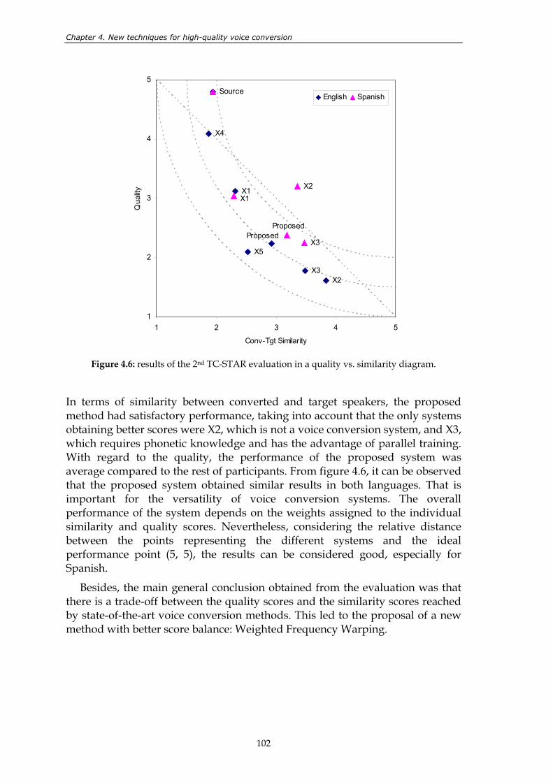
Chapter 4. New techniques for high-quality voice conversion
102
Proposed
X1
X5
X4
X3X2
Proposed
X1
Source
X3
X2
1
2
3
4
5
1 2 3 4 5
Conv-Tgt Similarity
Qua
lity
English Spanish
Figure 4.6: results of the 2nd TC-STAR evaluation in a quality vs. similarity diagram.
In terms of similarity between converted and target speakers, the proposed method had satisfactory performance, taking into account that the only systems obtaining better scores were X2, which is not a voice conversion system, and X3, which requires phonetic knowledge and has the advantage of parallel training. With regard to the quality, the performance of the proposed system was average compared to the rest of participants. From figure 4.6, it can be observed that the proposed system obtained similar results in both languages. That is important for the versatility of voice conversion systems. The overall performance of the system depends on the weights assigned to the individual similarity and quality scores. Nevertheless, considering the relative distance between the points representing the different systems and the ideal performance point (5, 5), the results can be considered good, especially for Spanish.
Besides, the main general conclusion obtained from the evaluation was that there is a trade-off between the quality scores and the similarity scores reached by state-of-the-art voice conversion methods. This led to the proposal of a new method with better score balance: Weighted Frequency Warping.
Intra-lingual and cross-lingual voice conversion using harmonic plus stochastic models
103
4.3. A new spectral conversion method
According to the objectives set at the beginning of this chapter, this section presents a new spectral envelope conversion method whose goal is to provide more natural converted sounds without loosing the degree of similarity reached by GMM-based transformations.
As it was mentioned above, frequency warping transformations are characterized by producing smaller quality degradation than the rest of existing methods. However, the converted-target similarity achieved by means of frequency warping is also low compared to that of other conversion methods. Weighted Frequency Warping is a new spectral envelope conversion method based on time-varying frequency warping transformations combined with GMMs. This combination brings together the advantages of both approaches.
4.3.1. Fundamentals of frequency warping transformations
The statistical transformation methods described in previous sections are suitable for all types of situations in which it is necessary to transform vectors. In the case of voice conversion, the problem is solved from a mathematical point of view, without considering the specific characteristics of the speech signals. In that sense, the frequency warping methods are more closely related to the acoustic theory of speech production, as they rely on the assumption that changes in the vocal tract length may produce a non-linear transformation of the formant frequencies.
Given two spectra X(f) and Y(f) for f in the range [0, fmax], the optimal frequency warping function w(f) can be defined as the non-linear continuous function of f that minimizes the error given by
( ) ( )( )( )∫ −= max
0
2loglogf
dffwYfXε (4.32)
The goal of voice conversion methods based on frequency warping is to transform the frequency axis of the source spectra by means of an adequate w(f) so that the converted spectra are maximally similar to the target spectra. Moreover, w(f) should not be constant: different phonemes may require different transformations. As it was explained in chapter 2, several implementations of this idea can be found in the literature.
The most important one is called Dynamic Frequency Warping (DFW) [Val92], and it operates with sampled short-time spectra obtained by STFT. Let us consider that x and y are p-dimensional vectors that contain the samples of two different magnitude spectra, log|X(f)| and log|Y(f)|, respectively. The DFW procedure determines the warping trajectory w=(i0, j0), (i1, j1), …, (iM, jM) for which the following distance measure is minimized:
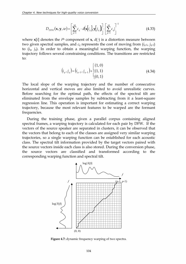
Chapter 4. New techniques for high-quality voice conversion
104
( ) [ ] [ ]( )1
11,,,
−
==
⋅
⋅= ∑∑
M
M
qqqqDFW cjidcwD yxyx (4.33)
where x[i] denotes the ith component of x, d(·) is a distortion measure between two given spectral samples, and cq represents the cost of moving from (iq-1, jq-1) to (iq, jq). In order to obtain a meaningful warping function, the warping trajectory follows several constraining conditions. The transitions are restricted to:
( ) ( )( )( )( )
+= −−
1 ,01 ,10 ,1
,, 11 qqqq jiji (4.34)
The local slope of the warping trajectory and the number of consecutive horizontal and vertical moves are also limited to avoid unrealistic curves. Before searching for the optimal path, the effects of the spectral tilt are eliminated from the envelope samples by subtracting from it a least-square regression line. This operation is important for estimating a correct warping trajectory, because the most relevant features to be warped are the formant frequencies.
During the training phase, given a parallel corpus containing aligned spectral frames, a warping trajectory is calculated for each pair by DFW. If the vectors of the source speaker are separated in clusters, it can be observed that the vectors that belong to each of the classes are assigned very similar warping trajectories, so a single warping function can be established for each acoustic class. The spectral tilt information provided by the target vectors paired with the source vectors inside each class is also stored. During the conversion phase, the source vectors are classified and transformed according to the corresponding warping function and spectral tilt.
Figure 4.7: dynamic frequency warping of two spectra.
(p-1, p-1)
f
f
log|X(f)|
(0, 0)
log|Y(f)|
Intra-lingual and cross-lingual voice conversion using harmonic plus stochastic models
105
There are other types of frequency warping techniques where parametric warping functions are estimated for each of the acoustic classes, like for example Vocal Tract Length Normalization (VTLN) [Sün03]. After having studied different types of warping function (power, quadratic, bilinear, piecewise linear), the author concludes that there is no need of using frequency transformations more complicated than
( )αf
fw = (4.35)
The optimum value of α is found for each of the acoustic classes, and during the conversion phase a smoothing technique is applied to the time-domain α-contour so that the transition between classes does not introduce discontinuities.
These techniques are very appropriate for modifying the gender or age of the speaker and for obtaining different voices from a single synthesis database efficiently. Nevertheless, they are reported to be weak for transforming voices into a specific target speaker’s voice. The most interesting property of such transformations is that they preserve very well the quality and naturalness of the synthetic converted speech. That is the reason why they have served as inspiration for designing the new transformation method proposed in the next section.
4.3.2. Weighted Frequency Warping (WFW)
Previous observations: phoneme classification by GMMs
The new spectral conversion method that is to be proposed in this section combines GMM-based and frequency-warping-based methods. In general, methods that use frequency warping functions consist of two main tasks:
Classification of the input frame.
Application of the warping function that corresponds to the assigned class.
The main disadvantage of clustering-based classification is that the transition between classes throughout the signal is abrupt, so discontinuities appear in the converted signal when the classes are assigned different transformation functions. Therefore, smoothing techniques are used to make the transformation function evolve slowly in time [Sün03a]. Instead of hard partitioning the acoustic space into m non-overlapping classes, GMMs perform a soft classification: each acoustic vector is assigned a certain probability of belonging to each of the m Gaussian components of the trained model. This property can be very interesting for improving frequency-warping systems and avoiding discontinuities. The question is how good GMMs are at classifying
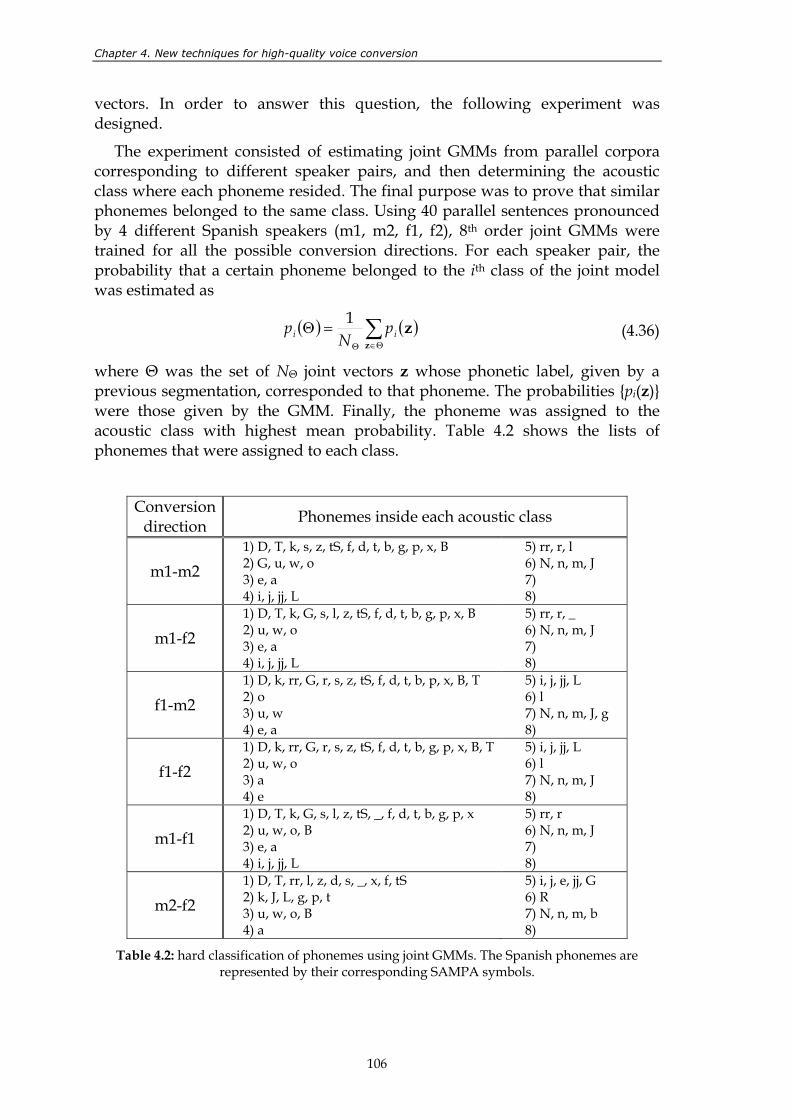
Chapter 4. New techniques for high-quality voice conversion
106
vectors. In order to answer this question, the following experiment was designed.
The experiment consisted of estimating joint GMMs from parallel corpora corresponding to different speaker pairs, and then determining the acoustic class where each phoneme resided. The final purpose was to prove that similar phonemes belonged to the same class. Using 40 parallel sentences pronounced by 4 different Spanish speakers (m1, m2, f1, f2), 8th order joint GMMs were trained for all the possible conversion directions. For each speaker pair, the probability that a certain phoneme belonged to the ith class of the joint model was estimated as
( ) ( )∑Θ∈Θ
=Θ
1z
zii pN
p (4.36)
where Θ was the set of NΘ joint vectors z whose phonetic label, given by a previous segmentation, corresponded to that phoneme. The probabilities pi(z) were those given by the GMM. Finally, the phoneme was assigned to the acoustic class with highest mean probability. Table 4.2 shows the lists of phonemes that were assigned to each class.
Conversion direction Phonemes inside each acoustic class
m1-m2 1) D, T, k, s, z, tS, f, d, t, b, g, p, x, B 2) G, u, w, o 3) e, a 4) i, j, jj, L
5) rr, r, l 6) N, n, m, J 7) 8)
m1-f2 1) D, T, k, G, s, l, z, tS, f, d, t, b, g, p, x, B 2) u, w, o 3) e, a 4) i, j, jj, L
5) rr, r, _ 6) N, n, m, J 7) 8)
f1-m2 1) D, k, rr, G, r, s, z, tS, f, d, t, b, p, x, B, T 2) o 3) u, w 4) e, a
5) i, j, jj, L 6) l 7) N, n, m, J, g 8)
f1-f2 1) D, k, rr, G, r, s, z, tS, f, d, t, b, g, p, x, B, T 2) u, w, o 3) a 4) e
5) i, j, jj, L 6) l 7) N, n, m, J 8)
m1-f1 1) D, T, k, G, s, l, z, tS, _, f, d, t, b, g, p, x 2) u, w, o, B 3) e, a 4) i, j, jj, L
5) rr, r 6) N, n, m, J 7) 8)
m2-f2 1) D, T, rr, l, z, d, s, _, x, f, tS 2) k, J, L, g, p, t 3) u, w, o, B 4) a
5) i, j, e, jj, G 6) R 7) N, n, m, b 8)
Table 4.2: hard classification of phonemes using joint GMMs. The Spanish phonemes are represented by their corresponding SAMPA symbols.
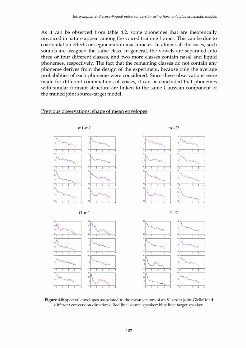
Intra-lingual and cross-lingual voice conversion using harmonic plus stochastic models
107
As it can be observed from table 4.2, some phonemes that are theoretically unvoiced in nature appear among the voiced training frames. This can be due to coarticulation effects or segmentation inaccuracies. In almost all the cases, such sounds are assigned the same class. In general, the vowels are separated into three or four different classes, and two more classes contain nasal and liquid phonemes, respectively. The fact that the remaining classes do not contain any phoneme derives from the design of the experiment, because only the average probabilities of each phoneme were considered. Since these observations were made for different combinations of voices, it can be concluded that phonemes with similar formant structure are linked to the same Gaussian component of the trained joint source-target model.
Previous observations: shape of mean envelopes
m1-m2
m1-f2
f1-m2
f1-f2
Figure 4.8: spectral envelopes associated to the mean vectors of an 8th order joint-GMM for 4
different conversion directions. Red line: source speaker; blue line: target speaker.
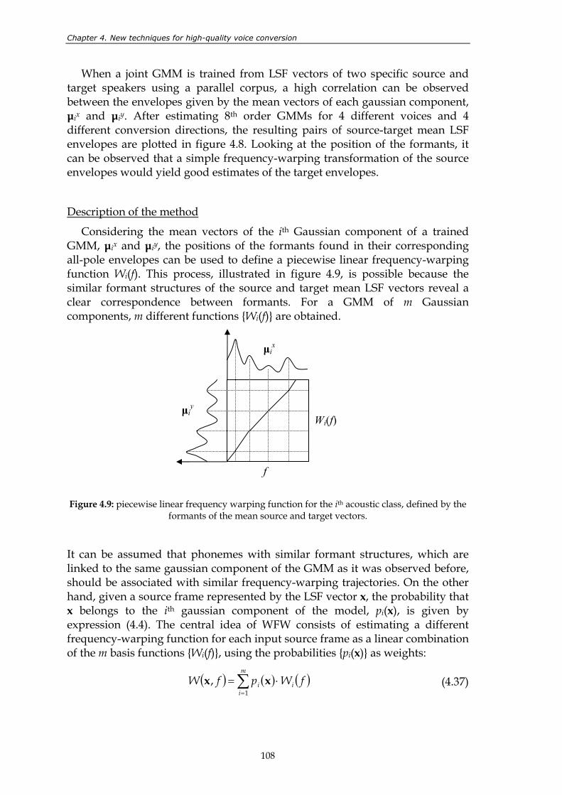
Chapter 4. New techniques for high-quality voice conversion
108
When a joint GMM is trained from LSF vectors of two specific source and target speakers using a parallel corpus, a high correlation can be observed between the envelopes given by the mean vectors of each gaussian component, µix and µiy. After estimating 8th order GMMs for 4 different voices and 4 different conversion directions, the resulting pairs of source-target mean LSF envelopes are plotted in figure 4.8. Looking at the position of the formants, it can be observed that a simple frequency-warping transformation of the source envelopes would yield good estimates of the target envelopes.
Description of the method
Considering the mean vectors of the ith Gaussian component of a trained GMM, µix and µiy, the positions of the formants found in their corresponding all-pole envelopes can be used to define a piecewise linear frequency-warping function Wi(f). This process, illustrated in figure 4.9, is possible because the similar formant structures of the source and target mean LSF vectors reveal a clear correspondence between formants. For a GMM of m Gaussian components, m different functions Wi(f) are obtained.
Figure 4.9: piecewise linear frequency warping function for the ith acoustic class, defined by the
formants of the mean source and target vectors.
It can be assumed that phonemes with similar formant structures, which are linked to the same gaussian component of the GMM as it was observed before, should be associated with similar frequency-warping trajectories. On the other hand, given a source frame represented by the LSF vector x, the probability that x belongs to the ith gaussian component of the model, pi(x), is given by expression (4.4). The central idea of WFW consists of estimating a different frequency-warping function for each input source frame as a linear combination of the m basis functions Wi(f), using the probabilities pi(x) as weights:
( ) ( ) ( )∑=
⋅=m
iii fWpfW
1, xx (4.37)
µix
µiy
f
Wi(f)
Intra-lingual and cross-lingual voice conversion using harmonic plus stochastic models
109
The main advantage of such frame-dependent frequency-warping function is evident: it does not contain important discontinuities, because the soft classification given by the GMM probabilities produces a smooth time-evolution of the transformation function. Therefore, the usage of further smoothing techniques is avoided. The spectrum of the current frame has to be transformed once its corresponding warping function W(x, f) has been calculated, so converted amplitude and phase envelopes, A’(f) and θ’(f), are obtained by applying it to the source envelopes:
( ) ( )( ) ( ) ( )( )fWffWAfA , , , 11 xx −− =′=′ θθ (4.38)
The source amplitude and phase envelopes can be extracted from the HSM parameters using the procedures detailed in chapter 3. Finally, the converted amplitudes Aj’(k) and vocal tract phases θj’(k) are obtained by resampling the warped envelopes at the harmonic frequencies1. It must be emphasized again that obviously this kind of transformation is applied only to voiced frames, where the harmonic component exists.
If the algorithm stopped here, the source voice would not be completely converted into the target voice, because the weighted frequency-warping procedure only reallocates the formants in the frequency axis, whereas their intensity, their bandwidth and the spectral tilt remain almost unmodified, yielding a different energy distribution in frequency. Manipulation of this kind of features directly on the warped spectra may negatively affect the naturalness of the converted signal. Fortunately, the information provided by the GMM estimated during the training phase allows a simple solution for this problem: the converted LSF vector F(x), obtained by means of the classical GMM conversion function (4.12), can be used to obtain a slightly different set of converted amplitudes Âj’(k). Obviously, if such amplitudes were taken as final converted amplitudes, there would be no difference between the system being described and a GMM-based baseline system, and this would imply loosing the benefits of frequency warping. However, an energy-correction filter can be defined by smoothing the gain filter defined by the discrete values Gj(k)=Âj’(k)/Aj’(k) in the frequency domain. The final converted amplitudes are obtained by multiplying Aj’(k) by the smoothed set of gain values. The energy of the total harmonic component is maintained with respect to the source frame. If the smoothing applied to the gain points is strong enough, the spectral tilt and the general energy distribution are slightly corrected without altering the small spectral shape details, so that there is not significant degradation of the naturalness of the resulting amplitude envelope.
With regard to the stochastic component, the same prediction method used in the baseline GMM-based system, given by expression (4.27), is adopted for WFW. The general block diagram of the new WFW method is shown in figure 4.10.
1 Here, the implementation of WFW is described according to the parameters of HSM, but the method is also compatible with many other speech models.
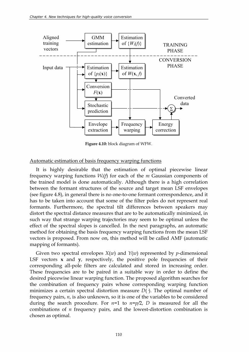
Chapter 4. New techniques for high-quality voice conversion
110
Figure 4.10: block diagram of WFW.
Automatic estimation of basis frequency warping functions
It is highly desirable that the estimation of optimal piecewise linear frequency warping functions Wi(f) for each of the m Gaussian components of the trained model is done automatically. Although there is a high correlation between the formant structures of the source and target mean LSF envelopes (see figure 4.8), in general there is no one-to-one formant correspondence, and it has to be taken into account that some of the filter poles do not represent real formants. Furthermore, the spectral tilt differences between speakers may distort the spectral distance measures that are to be automatically minimized, in such way that strange warping trajectories may seem to be optimal unless the effect of the spectral slopes is cancelled. In the next paragraphs, an automatic method for obtaining the basis frequency warping functions from the mean LSF vectors is proposed. From now on, this method will be called AMF (automatic mapping of formants).
Given two spectral envelopes X(w) and Y(w) represented by p-dimensional LSF vectors x and y, respectively, the positive pole frequencies of their corresponding all-pole filters are calculated and stored in increasing order. These frequencies are to be paired in a suitable way in order to define the desired piecewise linear warping function. The proposed algorithm searches for the combination of frequency pairs whose corresponding warping function minimizes a certain spectral distortion measure D(·). The optimal number of frequency pairs, n, is also unknown, so it is one of the variables to be considered during the search procedure. For n=1 to n=p/2, D is measured for all the combinations of n frequency pairs, and the lowest-distortion combination is chosen as optimal.
GMM estimation
Estimation of Wi(f)
Aligned training vectors
Input data Estimation of pi(x)
Estimation of W(x, f)
Frequency warping
Envelope extraction
Energy correction
Conversion F(x)
Stochastic prediction Σ
Converted data
TRAINING PHASE
CONVERSION PHASE
Intra-lingual and cross-lingual voice conversion using harmonic plus stochastic models
111
Let us now define the spectral distortion measure D for a certain set of n frequency pairs. The sub-indices 1…n are used for simplicity, although they do not necessarily correspond to the number of the pole they belong to (w1(x), w1(y)), …, (wn(x), wn(y)). This combination has valid physical meaning only if wi(x)
> wi–1(x) and wi(y) > wi–1(y) for every i, so it can be directly discarded if this condition is not satisfied. First, the pairs (0, 0) and (π, π) are added at both ends of the sequence. The associated warping function can be expressed as
( )
<<+
<<+<<+
=
πwwBwA
wwwBwAwwBwA
wW
xnnn
xx
x
)(
)(2
)(111
)(100 0
M (4.39)
The parameters Ai and Bi verify
)()()()(
1
)()(1 , x
iiy
iixi
xi
yi
yi
i wAwBwwwwA −=
−−
=+
+ (4.40)
where w0(x) = w0(y) = 0 and wn+1(x) = wn+1(y) = π. The problem of computing the spectral distortion D can be solved separately for each interval:
( ) ( )( ) ( )
( ) ( ) ( )( ) ( ) ( )( )[ ]∑=
+′′++⋅+=
=n
iiimmiiimmii
wW
BwAYwXDBwAYwXDA
wYwXD
0,,1
,
α (4.41)
where
( ) ( ) ( ) ( )( ) ( ) ( ) ( )wYwYwXwX
wYwYwXwX
mdwd
mmdwd
m
mm
=′=′==
,log ,log
( ) ( )( ) ( ) ( )[ ]∫+ −=
)(1
)(
2,x
i
xi
w
w mmmmi dwwYwXwYwXD (4.42)
The reason for including the derivative of the magnitude spectrum is that the resulting function is less sensitive to the differences in spectral tilt. The factor (1+Ai) was included in expression (4.41) for optimizing simultaneously not only the spectral distortion between X(w) and Y(W(w)) but also the distortion between X(W-1(w)) and Y(w). As the warping function is linear within the ith interval, the ratio between both distances is exactly Ai. It is easy to prove that the following general statement is true:
( ) ( )[ ] ( ) ( )[ ]∫∫ −⋅=−1
0
2
0
2 dwAwYwXAdwwYX mm
A
mAw
m (4.43)
It is possible to obtain analytical expressions for the spectral distortion using the magnitude response of the involved all-pole filters, but the problem is much more easily solved if the magnitude spectra are modelled through cepstral decomposition. Ignoring the first cepstral coefficient, which contains only the energy, they can be expressed as
( ) ( ) ∑∑ ==≈≈
p
j jmp
j jm jwdwYjwcwX11
cos ,cos (4.44)
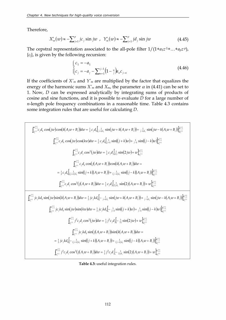
Chapter 4. New techniques for high-quality voice conversion
112
Therefore,
( ) ( ) ∑∑ ==−≈′−≈′ p
j jmp
j jm jwjdwYjwjcwX11
sin ,sin (4.45)
The cepstral representation associated to the all-pole filter 1/(1+a1z-1+…+apz-p), cj, is given by the following recursion:
( )
−−−=
−=
∑ −
= −1
1
11
1j
n njnjn
jj caac
ac (4.46)
If the coefficients of X’m and Y’m are multiplied by the factor that equalizes the energy of the harmonic sums X’m and Xm, the parameter α in (4.41) can be set to 1. Now, D can be expressed analytically by integrating sums of products of cosine and sine functions, and it is possible to evaluate D for a large number of n-length pole frequency combinations in a reasonable time. Table 4.3 contains some integration rules that are useful for calculating D.
( ) ( )( ) ( )( ) ( )( )[ ] )(1)(
)(1
)( sinsincoscos 1121
xi
xiii
xi
xi
w
wiikAjiikAjkj
w
w iikj BwAkjwBwAkjwdcdwBwAkjwdc ++ +−+++=+ −+∫
( ) ( ) ( )( ) ( )( )[ ] )(1)(
)(1
)( sinsincoscos 1121
xix
i
xi
xi
w
wkjkjkj
w
w kj wkjwkjdcdwkwjwdc ++ −++= −+∫
( ) ( )[ ] )(1)(
)(1
)( 2sincos 21
212
xi
xi
xi
xi
w
wjjj
w
w jj wjwdcdwjwdc ++ +=∫
( )( ) ( )( )
( ) ( )( )( ) ( ) ( )( )( )[ ] )(1)(
)(1
)(
sinsin
coscos
1121
xix
iii
xi
xi
w
wiiAkjiiAkjkj
w
w iiiikj
BwAkjBwAkjdc
dwBwAkBwAjdc
+
+
+−+++=
=++
−+
∫
( )( ) ( )( )[ ] )(1)(
)(1
)( 2sincos 21
212 x
ix
ii
xi
xi
w
wiijAjj
w
w iijj wBwAjdcdwBwAjdc ++ ++=+∫
( ) ( )( ) ( )( ) ( )( )[ ] )(1)(
)(1
)( sinsinsinsin 1121
xi
xiii
xi
xi
w
wiikAjiikAjkj
w
w iikj BwAkjwBwAkjwkdjcdwBwAkjwkdjc ++ +−+++−=+ −+∫
( ) ( ) ( )( ) ( )( )[ ] )(1)(
)(1
)( sinsinsinsin 1121
xix
i
xi
xi
w
wkjkjkj
w
w kj wkjwkjkdjcdwkwjwkdjc ++ −++−= −+∫
( ) ( )[ ] )(1)(
)(1
)( 2sincos 212
2122 x
ix
i
xi
xi
w
wjjj
w
w jj wjwdcjdwjwdcj ++ +−=∫
( )( ) ( )( )
( ) ( )( )( ) ( ) ( )( )( )[ ] )(1)(
)(1
)(
sinsin
sinsin
1121
xi
xiii
xi
xi
w
wiiAkjiiAkjkj
w
w iiiikj
BwAkjBwAkjkdjc
dwBwAkBwAjkdjc
+
+
+−+++−=
=++
−+
∫
( )( ) ( )( )[ ] )(1)(
)(1
)( 2sincos 212
2122 x
ix
ii
xi
xi
w
wiijAjj
w
w iijj wBwAjdcjdwBwAjdcj ++ ++−=+∫
Table 4.3: useful integration rules.
Intra-lingual and cross-lingual voice conversion using harmonic plus stochastic models
113
Automatic estimation of basis frequency warping functions (ii)
Although the automatic method described above imitates the manual pairing of poles, it relies on the assumption that the mean vectors characterizing each of the acoustic classes, apart from their mathematical meaning, have certain physical meaning. In order to obtain more realistic frequency warping curves for each acoustic class, it would be interesting to establish the optimal mapping by considering the characteristics of all the vectors inside the class, not only of the mean vectors. For this reason, the following method based on weighted histograms (from now on, WH) was also investigated. Given the training vectors of the source and target speakers, x and y, and the parameters of their individual mth-order GMMs obtained from a joint-density model, the idea of the WH method is to estimate the FW basis functions from m source histograms hix and their corresponding m target histograms hiy, one source and target histogram per class, representing the probability of finding a pole inside a certain frequency region if the current frame belongs to that class. Next, the procedure for calculating the source histograms hix is described:
1. All the histograms are initialized by assigning a zero value to all the frequency regions. In this case, the analysis band (0-5 KHz) is divided into 50Hz-wide regions.
2. For each LSF vector x, the pole frequencies of the corresponding all-pole filter are calculated and stored. It is assumed that all the poles have the same importance for the calculation of the histograms, regardless of their intensity or bandwidth.
3. For each x, the m probabilities pi(x) are calculated by means of equation (4.4) using the individual GMM of the source speaker (remember that pi(x) represents the probability of x to belong to the ith class).
4. For i=1 to i=m and for every x, the regions of hix containing the poles of x are incremented by pi(x). Thus, the contribution of x affects all the histograms in a weighted manner.
5. Finally, each histogram is normalized so that its sum is 1.
The target histograms are calculated in a similar way. Once all the histograms have been obtained, the warping functions Wi(f) to be used for transformation are determined by aligning hix and hiy through DFW. One of the main disadvantages of applying DFW directly to spectra is that strong spectral tilt differences have a harmful effect on the resulting warping paths. In this case, the spectral tilt has no influence on the histograms, so the resulting trajectories are reliable.
In order to decide which of the described automatic methods was better for determining the basis frequency warping functions, an objective test similar to those of the previous sections was carried out. It consisted of computing the mean cepstral distance between converted and target envelopes for a 10-sentence-length parallel test corpus. 4 voices and 40 sentences per voice were used for automatically training the 12 possible voice conversion functions.
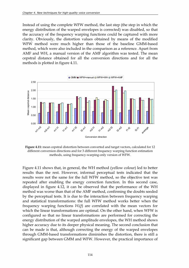
Chapter 4. New techniques for high-quality voice conversion
114
Instead of using the complete WFW method, the last step (the step in which the energy distribution of the warped envelopes is corrected) was disabled, so that the accuracy of the frequency warping functions could be captured with more clarity. Obviously, the distortion values obtained by means of the modified WFW method were much higher than those of the baseline GMM-based method, which were also included in the comparison as a reference. Apart from AMF and WH, a manual version of the AMF algorithm was tested. The mean cepstral distance obtained for all the conversion directions and for all the methods is plotted in figure 4.11.
0.00
0.50
1.00
1.50
2.00
2.50
m1-m2
m2-m1
m1-f1
f1-m1
m1-f2
f2-m1
m2-f1
f1-m2
m2-f2
f2-m2
f1-f2
f2-f1
avera
ge
Conversion direction
Mea
n ce
pstra
l dis
tanc
e
GMM WFW+manual WFW+WH WFW+AMF
Figure 4.11: mean cepstral distortion between converted and target vectors, calculated for 12
different conversion directions and for 3 different frequency warping function estimation methods, using frequency-warping-only version of WFW.
Figure 4.11 shows that, in general, the WH method (yellow colour) led to better results than the rest. However, informal perceptual tests indicated that the results were not the same for the full WFW method, so the objective test was repeated after enabling the energy correction function. In this second case, displayed in figure 4.12, it can be observed that the performance of the WH method was worse than that of the AMF method, confirming the doubts seeded by the perceptual tests. It is due to the interaction between frequency warping and statistical transformations: the full WFW method works better when the frequency warping functions Wi(f) are correlated with the mean vectors for which the linear transformations are optimal. On the other hand, when WFW is configured so that no linear transformations are performed for correcting the energy distribution of the warped amplitude envelopes, the WH method shows higher accuracy due to its deeper physical meaning. The second conclusion that can be made is that, although correcting the energy of the warped envelopes through GMM-based transformations diminishes the distortion, there is still a significant gap between GMM and WFW. However, the practical importance of
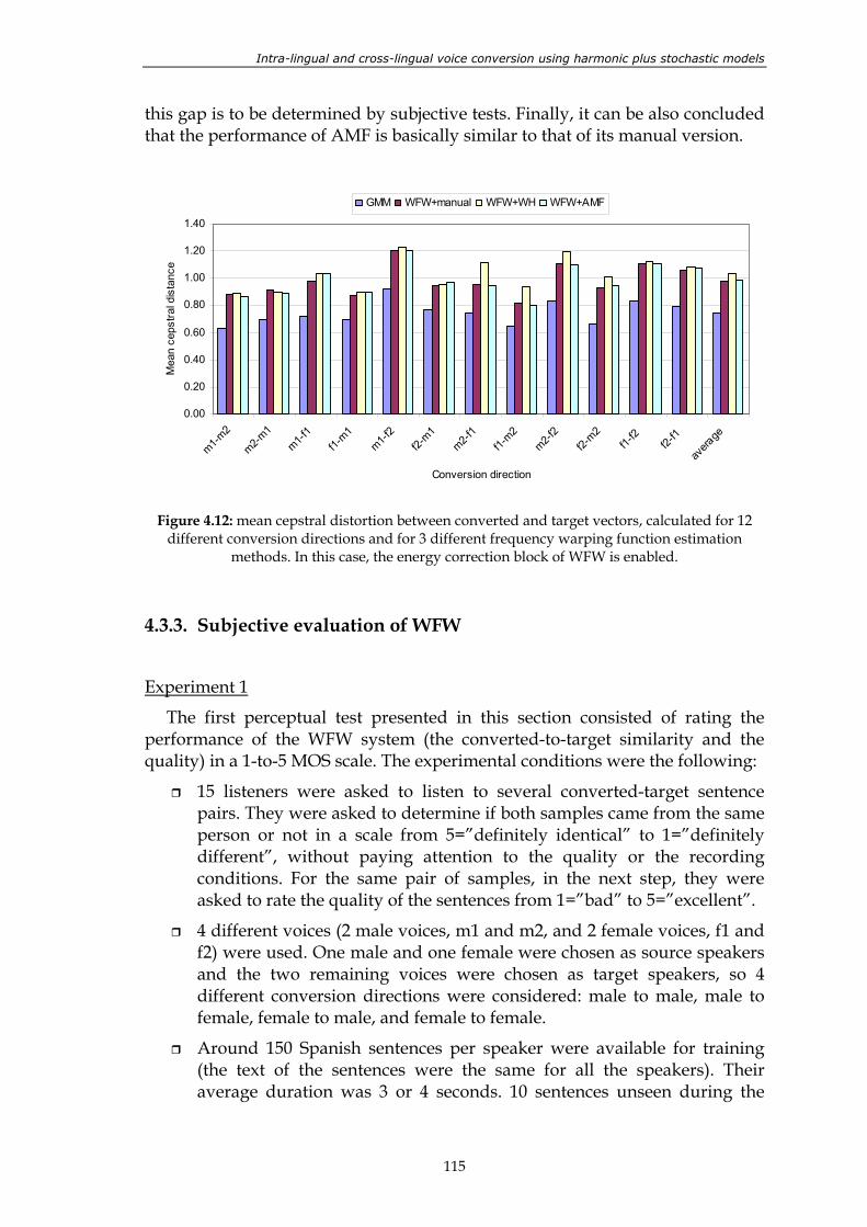
Intra-lingual and cross-lingual voice conversion using harmonic plus stochastic models
115
this gap is to be determined by subjective tests. Finally, it can be also concluded that the performance of AMF is basically similar to that of its manual version.
0.00
0.20
0.40
0.60
0.80
1.00
1.20
1.40
m1-m2
m2-m1
m1-f1
f1-m1
m1-f2
f2-m1
m2-f1
f1-m2
m2-f2
f2-m2
f1-f2
f2-f1
avera
ge
Conversion direction
Mea
n ce
pstra
l dis
tanc
e
GMM WFW+manual WFW+WH WFW+AMF
Figure 4.12: mean cepstral distortion between converted and target vectors, calculated for 12
different conversion directions and for 3 different frequency warping function estimation methods. In this case, the energy correction block of WFW is enabled.
4.3.3. Subjective evaluation of WFW
Experiment 1
The first perceptual test presented in this section consisted of rating the performance of the WFW system (the converted-to-target similarity and the quality) in a 1-to-5 MOS scale. The experimental conditions were the following:
15 listeners were asked to listen to several converted-target sentence pairs. They were asked to determine if both samples came from the same person or not in a scale from 5=”definitely identical” to 1=”definitely different”, without paying attention to the quality or the recording conditions. For the same pair of samples, in the next step, they were asked to rate the quality of the sentences from 1=”bad” to 5=”excellent”.
4 different voices (2 male voices, m1 and m2, and 2 female voices, f1 and f2) were used. One male and one female were chosen as source speakers and the two remaining voices were chosen as target speakers, so 4 different conversion directions were considered: male to male, male to female, female to male, and female to female.
Around 150 Spanish sentences per speaker were available for training (the text of the sentences were the same for all the speakers). Their average duration was 3 or 4 seconds. 10 sentences unseen during the
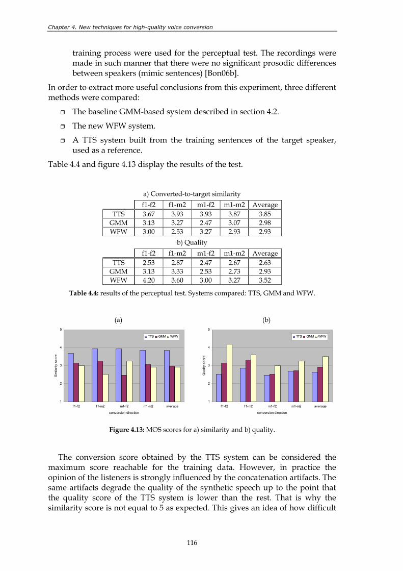
Chapter 4. New techniques for high-quality voice conversion
116
training process were used for the perceptual test. The recordings were made in such manner that there were no significant prosodic differences between speakers (mimic sentences) [Bon06b].
In order to extract more useful conclusions from this experiment, three different methods were compared:
The baseline GMM-based system described in section 4.2.
The new WFW system.
A TTS system built from the training sentences of the target speaker, used as a reference.
Table 4.4 and figure 4.13 display the results of the test.
a) Converted-to-target similarity f1-f2 f1-m2 m1-f2 m1-m2 Average
TTS 3.67 3.93 3.93 3.87 3.85 GMM 3.13 3.27 2.47 3.07 2.98 WFW 3.00 2.53 3.27 2.93 2.93
b) Quality f1-f2 f1-m2 m1-f2 m1-m2 Average
TTS 2.53 2.87 2.47 2.67 2.63 GMM 3.13 3.33 2.53 2.73 2.93 WFW 4.20 3.60 3.00 3.27 3.52
Table 4.4: results of the perceptual test. Systems compared: TTS, GMM and WFW.
(a)
1
2
3
4
5
f1-f2 f1-m2 m1-f2 m1-m2 average
conversion direction
Sim
ilarit
y sc
ore
TTS GMM WFW
(b)
1
2
3
4
5
f1-f2 f1-m2 m1-f2 m1-m2 average
conversion direction
Qua
lity s
core
TTS GMM WFW
Figure 4.13: MOS scores for a) similarity and b) quality.
The conversion score obtained by the TTS system can be considered the maximum score reachable for the training data. However, in practice the opinion of the listeners is strongly influenced by the concatenation artifacts. The same artifacts degrade the quality of the synthetic speech up to the point that the quality score of the TTS system is lower than the rest. That is why the similarity score is not equal to 5 as expected. This gives an idea of how difficult
Intra-lingual and cross-lingual voice conversion using harmonic plus stochastic models
117
it is to reach a similarity score higher than 4. Now, concerning the voice conversion methods, a small loss of conversion accuracy from GMM to WFW can be observed. This is a consequence of the fact that small spectral details of the source speaker persist when the frequency warping procedure is applied, and also that the quality increment achieved by WFW makes the differences between speakers more visible. Looking at the different conversion directions it can be seen that the main significant differences are located in the cross-gender conversion cases. In particular, WFW fails when converting from female to male. The reason is the strong contrast in f0 between these specific speakers, because the source spectral envelopes are defined by few harmonics, whereas a high number of target harmonics have to be extracted from them. Looking at the quality scores, it can be seen that the quality increment from GMM to WFW is very significant. Furthermore, the improvements are visible and consistent in every conversion direction. Some other informal tests have been carried out to evaluate the WFW system using less training data, and the results are similar to those displayed in table 4.4. As a conclusion, it can be stated that WFW successfully accomplishes the objectives proposed at the beginning of this chapter.
Experiment 2
The implemented WFW system was one of the competitors that participated in the third Evaluation Campaign of the European project TC-STAR [Mos07]. The evaluation conditions were basically the same as in the second evaluation campaign (section 4.2):
The converted-to-target similarity and the quality were rated by 20 listeners using a 1-to-5 MOS scale.
4 different conversion directions were considered again: male to male, male to female, female to male, and female to female.
All the speakers involved were bilingual: for each speaker, around 150 Spanish sentences and 150 English sentences were available for training. The average duration of the sentences was around 3 or 4 seconds. 10 sentences unseen during training were used for the perceptual test. The same sentences were uttered by all the speakers, so that a parallel corpus could be created. The recordings were made in such manner that there were no significant prosodic differences between speakers (mimic sentences) [Bon06b].
The WFW system was configured to use 8th order GMMs for the evaluation. The results of the evaluation are shown in table 4.5, which has been extracted from the public report in [Mos07]. The rest of the systems participating in the evaluation are given fictitious names here (which may not correspond to those used in section 4.2). The same results are displayed in figure 4.14, where each system is represented by a point whose coordinates correspond to its similarity and quality scores.
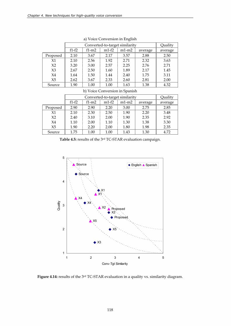
Chapter 4. New techniques for high-quality voice conversion
118
a) Voice Conversion in English Converted-to-target similarity Quality
f1-f2 f1-m2 m1-f2 m1-m2 average average Proposed 2.10 3.67 2.17 3.57 2.88 2.50
X1 X2 X3 X4 X5
2.10 3.20 2.67 1.64 2.62
2.56 3.00 2.50 1.50 3.67
1.92 2.57 1.60 1.44 2.33
2.71 2.25 1.89 2.40 2.60
2.32 2.76 2.17 1.75 2.81
3.63 2.71 1.45 3.11 2.00
Source 1.90 1.00 1.00 1.63 1.38 4.32 b) Voice Conversion in Spanish Converted-to-target similarity Quality
f1-f2 f1-m2 m1-f2 m1-m2 average average Proposed 2.90 2.90 2.20 3.00 2.75 2.85
X1 X2 X4 X5
2.10 2.40 1.10 1.90
2.30 3.10 2.00 2.20
2.50 2.00 1.10 2.00
1.90 1.90 1.30 1.80
2.20 2.35 1.38 1.98
3.48 2.92 3.30 2.35
Source 1.75 1.00 1.00 1.43 1.30 4.72
Table 4.5: results of the 3rd TC-STAR evaluation campaign.
X2Proposed
X4
X5
X3
X1
Source
X4
X2 Proposed
X5
X1
Source
1
2
3
4
5
1 2 3 4 5
Conv-Tgt Similarity
Qua
lity
English Spanish
Figure 4.14: results of the 3rd TC-STAR evaluation in a quality vs. similarity diagram.
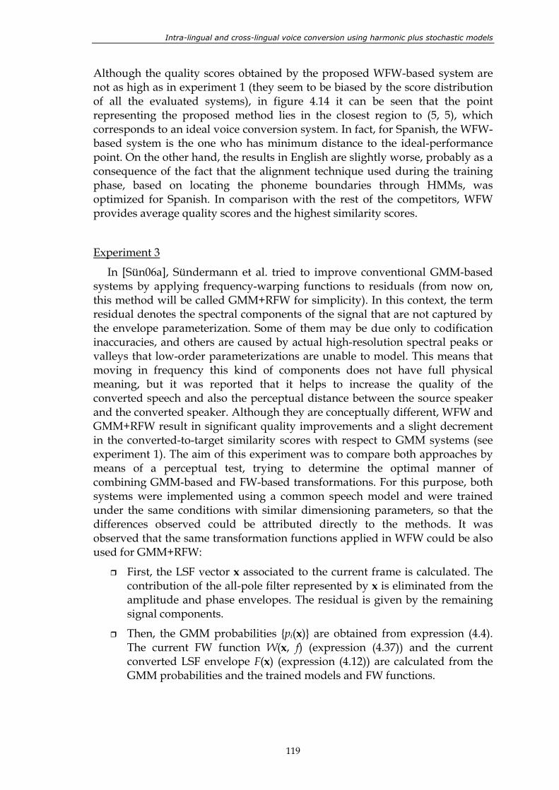
Intra-lingual and cross-lingual voice conversion using harmonic plus stochastic models
119
Although the quality scores obtained by the proposed WFW-based system are not as high as in experiment 1 (they seem to be biased by the score distribution of all the evaluated systems), in figure 4.14 it can be seen that the point representing the proposed method lies in the closest region to (5, 5), which corresponds to an ideal voice conversion system. In fact, for Spanish, the WFW-based system is the one who has minimum distance to the ideal-performance point. On the other hand, the results in English are slightly worse, probably as a consequence of the fact that the alignment technique used during the training phase, based on locating the phoneme boundaries through HMMs, was optimized for Spanish. In comparison with the rest of the competitors, WFW provides average quality scores and the highest similarity scores.
Experiment 3
In [Sün06a], Sündermann et al. tried to improve conventional GMM-based systems by applying frequency-warping functions to residuals (from now on, this method will be called GMM+RFW for simplicity). In this context, the term residual denotes the spectral components of the signal that are not captured by the envelope parameterization. Some of them may be due only to codification inaccuracies, and others are caused by actual high-resolution spectral peaks or valleys that low-order parameterizations are unable to model. This means that moving in frequency this kind of components does not have full physical meaning, but it was reported that it helps to increase the quality of the converted speech and also the perceptual distance between the source speaker and the converted speaker. Although they are conceptually different, WFW and GMM+RFW result in significant quality improvements and a slight decrement in the converted-to-target similarity scores with respect to GMM systems (see experiment 1). The aim of this experiment was to compare both approaches by means of a perceptual test, trying to determine the optimal manner of combining GMM-based and FW-based transformations. For this purpose, both systems were implemented using a common speech model and were trained under the same conditions with similar dimensioning parameters, so that the differences observed could be attributed directly to the methods. It was observed that the same transformation functions applied in WFW could be also used for GMM+RFW:
First, the LSF vector x associated to the current frame is calculated. The contribution of the all-pole filter represented by x is eliminated from the amplitude and phase envelopes. The residual is given by the remaining signal components.
Then, the GMM probabilities pi(x) are obtained from expression (4.4). The current FW function W(x, f) (expression (4.37)) and the current converted LSF envelope F(x) (expression (4.12)) are calculated from the GMM probabilities and the trained models and FW functions.
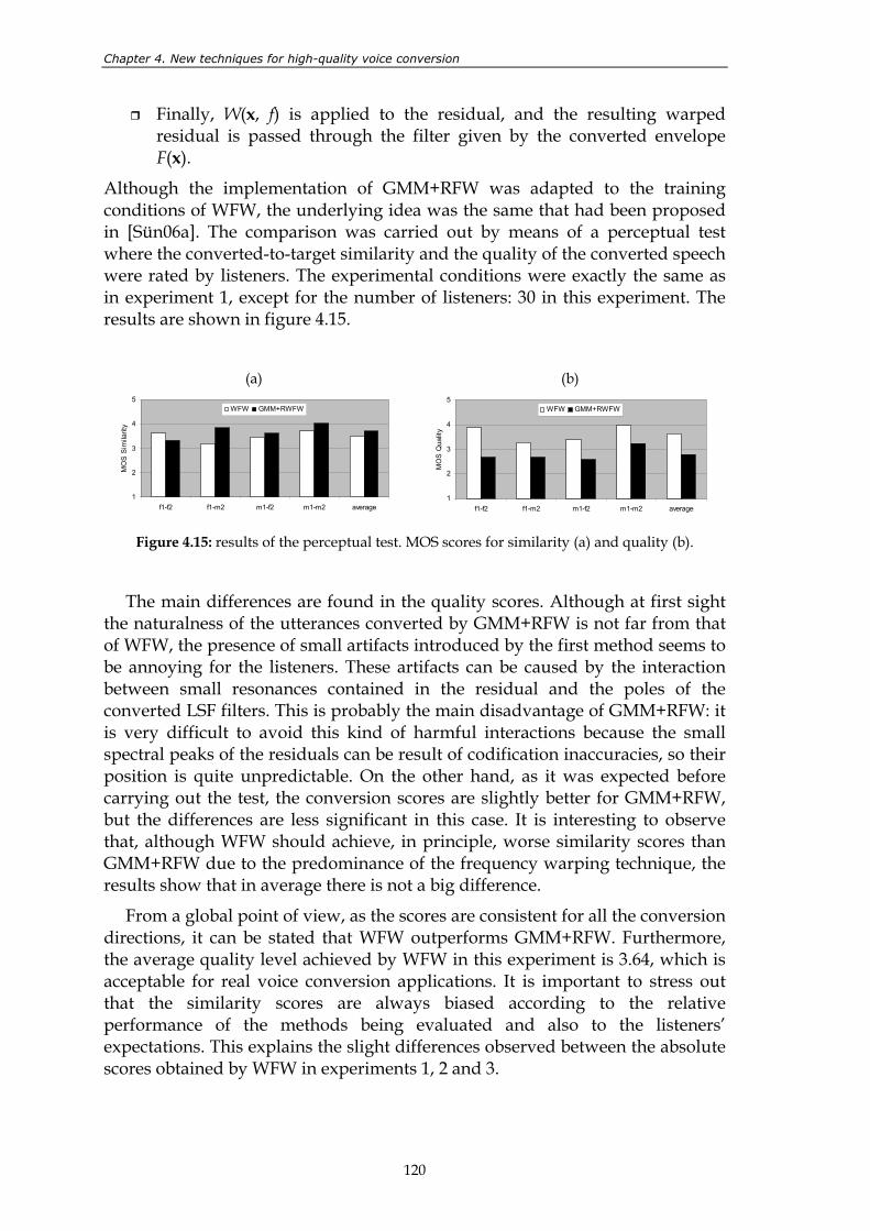
Chapter 4. New techniques for high-quality voice conversion
120
Finally, W(x, f) is applied to the residual, and the resulting warped residual is passed through the filter given by the converted envelope F(x).
Although the implementation of GMM+RFW was adapted to the training conditions of WFW, the underlying idea was the same that had been proposed in [Sün06a]. The comparison was carried out by means of a perceptual test where the converted-to-target similarity and the quality of the converted speech were rated by listeners. The experimental conditions were exactly the same as in experiment 1, except for the number of listeners: 30 in this experiment. The results are shown in figure 4.15.
(a)
1
2
3
4
5
f1-f2 f1-m2 m1-f2 m1-m2 average
MO
S S
imila
rity
WFW GMM+RWFW
(b)
1
2
3
4
5
f1-f2 f1-m2 m1-f2 m1-m2 average
MO
S Q
ualit
y
WFW GMM+RWFW
Figure 4.15: results of the perceptual test. MOS scores for similarity (a) and quality (b).
The main differences are found in the quality scores. Although at first sight the naturalness of the utterances converted by GMM+RFW is not far from that of WFW, the presence of small artifacts introduced by the first method seems to be annoying for the listeners. These artifacts can be caused by the interaction between small resonances contained in the residual and the poles of the converted LSF filters. This is probably the main disadvantage of GMM+RFW: it is very difficult to avoid this kind of harmful interactions because the small spectral peaks of the residuals can be result of codification inaccuracies, so their position is quite unpredictable. On the other hand, as it was expected before carrying out the test, the conversion scores are slightly better for GMM+RFW, but the differences are less significant in this case. It is interesting to observe that, although WFW should achieve, in principle, worse similarity scores than GMM+RFW due to the predominance of the frequency warping technique, the results show that in average there is not a big difference.
From a global point of view, as the scores are consistent for all the conversion directions, it can be stated that WFW outperforms GMM+RFW. Furthermore, the average quality level achieved by WFW in this experiment is 3.64, which is acceptable for real voice conversion applications. It is important to stress out that the similarity scores are always biased according to the relative performance of the methods being evaluated and also to the listeners’ expectations. This explains the slight differences observed between the absolute scores obtained by WFW in experiments 1, 2 and 3.
Intra-lingual and cross-lingual voice conversion using harmonic plus stochastic models
121
4.4. Conclusions
In this chapter, the problem of increasing the quality of the converted speech without worsening the conversion performance has been faced.
As a starting point, a state-of-the-art voice conversion system based on GMMs and harmonic-stochastic speech modeling has been implemented and evaluated. The performance of the system is satisfactory in terms of similarity between converted and target voices, but the results obtained in the 2nd evaluation campaign of the TC-STAR project show that the quality scores are low compared to other competitors.
It was observed that each of the acoustic classes modelled by a GMM contains vectors coming from phonemes with similar spectral characteristics. In addition, it was also observed that if a joint GMM is trained from aligned vectors of two different speakers, the mean vectors inside each acoustic class also have a similar formant structure, up to the point that their relationship seems to be well captured by a piecewise linear frequency warping function estimated from the formant frequencies. Therefore, a new method for converting spectral envelopes called Weighted Frequency Warping was proposed. WFW assigns an optimal frequency warping function Wi(f) to each of the acoustic classes, so during the conversion step a frame-dependent time-varying frequency warping function is obtained by combining the set of basis functions Wi(f) according to the probability of the current frame to belong to each of the acoustic classes. Finally, conventional statistical methods based on GMM transformations are applied to correct the energy of the warped spectra, so that not only the position of the formants is modified, but also their intensity.
The experiments carried out for evaluating the new voice conversion method prove that a good balance between similarity and quality scores is obtained. The similarity scores of WFW and those of the baseline GMM-based system are almost the same, whereas in WFW there is a significant improvement in the quality of the converted utterances. The results of the 3rd evaluation campaign of the TC-STAR project confirm that WFW has a very good performance compared to the rest of competitors, especially in Spanish, which is the language for which the system was optimized. On the other hand, WFW has better overall performance than other techniques that combine GMM-based and FW-based transformations. The absolute quality scores that characterize WFW allow using this method for real-life applications.
The main limitation of the new voice conversion system is that it needs parallel corpora to train the transformation functions, and so far it is incompatible with, for instance, cross-lingual applications. Is there any convincing solution for this problem? The next chapter gives an answer to this question.
Chapter 4. New techniques for high-quality voice conversion
122
Related publications
H. Duxans, D. Erro, J. Pérez, F. Diego, A. Bonafonte, A. Moreno, “Voice Conversion of Non-Aligned Data using Unit Selection”, TC-Star Workshop on Speech-to-Speech Translation. Barcelona, Spain. June 2006.
D. Erro, A. Moreno, “Sistema de Síntesis Armónico/Estocástico en modo Pitch-Asíncrono aplicado a Conversión de Voz”, IV Jornadas en Tecnologías del Habla, IV JTH, Zaragoza, Spain. November 2006.
A. Moreno, A. Bonafonte, J. Adell, P.D. Agüero, I. Esquerra, D. Erro, J. Pérez, T. Polyakova, H.U. Hain, J. Racky, D. Sündermann, I. Kiss, R. Fernández, Z. Shuang, “Deliverable D29. TTS: Progress Report”, technical report of the project TC-STAR (Technology and Corpora for Speech to Speech Translation). 2007.
D. Erro, A. Moreno, “Weighted Frequency Warping for Voice Conversion”, InterSpeech 2007, EuroSpeech. Antwerp, Belgium. August 2007.
D. Erro, T. Polyakova, A. Moreno, “On combining statistical methods and frequency warping for high-quality voice conversion”, Proc. ICASSP 2008. Las Vegas, USA. March 2008.
123
5. Alignment of frames for non-parallel training
Most of the relevant spectral conversion methods found in the literature are designed for training conversion functions from a set of paired phonetically-equivalent acoustic vectors obtained from the source and target speakers, respectively. For instance, all the systems that are based on GMMs, including those presented in chapter 4, require a set of paired source-target vectors from which the optimal transformation is learnt. The process responsible for pairing of the vectors from a given speech database is called alignment (see figure 5.1).
The alignment procedure strongly influences the versatility of the whole voice conversion system. It is easy to obtain a valid alignment if the involved speakers are asked to pronounce the same training sentences. In this situation, we say that a parallel training corpus is available, and, as it was explained in chapter 2, the acoustic vectors can be paired by techniques like DTW or HMM-based automatic segmentation. Nevertheless, in real-life situations it is not possible to record parallel training corpora for any random pair of speakers. Cross-lingual voice conversion poses even a greater challenge, since the sentences uttered in different languages cannot be parallel. Furthermore, one of the languages can have some basic sound units or phonemes that do not exist in the other one. The procedure of training conversion functions from non-parallel corpora is referred to as non-parallel training and, for right now, there was no satisfactory solution proposed.
This chapter presents a new frame alignment method that is compatible with intra-lingual and cross-lingual voice conversion under non-parallel-training conditions. The chapter is structured as follows.
In section 5.1, some previous solutions to the non-parallel training problem are reviewed and discussed, included some preliminary results obtained during the elaboration of this thesis.
In section 5.2, a new iterative frame alignment method is proposed. Different aspects about convergence, optimization and performance of the method are carefully analyzed and discussed.
In section 5.3, the method is evaluated under intra-lingual and cross-lingual conditions by means of perceptual tests.
In section 5.4, the main conclusions of this chapter are summarized.
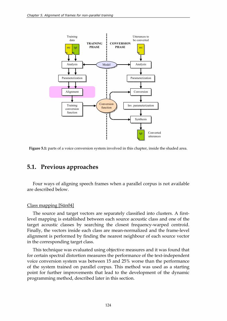
Chapter 5. Alignment of frames for non-parallel training
124
Figure 5.1: parts of a voice conversion system involved in this chapter, inside the shaded area.
5.1. Previous approaches
Four ways of aligning speech frames when a parallel corpus is not available are described below.
Class mapping [Sün04]
The source and target vectors are separately classified into clusters. A first-level mapping is established between each source acoustic class and one of the target acoustic classes by searching the closest frequency-warped centroid. Finally, the vectors inside each class are mean-normalized and the frame-level alignment is performed by finding the nearest neighbour of each source vector in the corresponding target class.
This technique was evaluated using objective measures and it was found that for certain spectral distortion measures the performance of the text-independent voice conversion system was between 15 and 25% worse than the performance of the system trained on parallel corpus. This method was used as a starting point for further improvements that lead to the development of the dynamic programming method, described later in this section.
Converted utterances
Analysis
Parameterization
Alignment
Training conversion
function
Analysis
Parameterization
Conversion
Synthesis
tgt
Inv. parameterization
TRAINING PHASE
CONVERSION PHASE src tgt
Training data
Utterances to be converted
src
Model
Conversion function
Intra-lingual and cross-lingual voice conversion using harmonic plus stochastic models
125
Speech recognition [Ye04b]
A speech recognizer based on speaker-independent HMMs is used to label all the source and target frames with a state index. Given the state sequence of one speaker, the alignment procedure consists of finding longest matching state sub-sequences from the other speaker until all the frames are paired.
The HMMs used for this task are valid for intra-lingual alignment. Although multilingual HMMs were also used in polyglot voice conversion systems [Lat06], the suitability of such models for cross-lingual alignment tasks has not been proved yet.
Pseudo-parallel corpus created by a TTS
This technique consists of using a TTS system to generate the same sentences uttered by the target speaker by concatenating speech units of the source speaker [Enn05, Dux06b]. The pseudo-parallel corpus obtained allows using standard frame alignment methods such as DTW. However, this solution can be put into practice only under certain conditions:
The TTS system uses linguistic knowledge to generate artificial sentences, so the language of the desired output sentence has to be the same as the language of the recorded units. Therefore, this kind of technique is restricted to intra-lingual context, unless at least one of the involved speakers is bilingual.
The size of the training corpus has to be large enough to build a TTS system. Otherwise, if only few minutes of audio are available for building the TTS that acts as source speaker, the resulting low-quality synthetic speech leads to a distorted conversion function that introduces artifacts into the converted speech.
During the 2nd evaluation campaign of the European TC-STAR project, several voice conversion systems were evaluated by means of perceptual tests. As mentioned in section 4.2, the baseline voice conversion system developed in this thesis was one of the participants of the evaluation. In this system, a TTS was applied to obtain pseudo-parallel corpora instead of using parallel corpora for training. Furthermore, the system participated in the cross-lingual evaluation. All the speakers recorded for the evaluation database were bilingual, so in order for the system to operate in cross-lingual mode, the transformation functions were trained for one language and then were applied to convert sentences uttered in the other language. The results of the evaluation are shown in table 5.2 (the results of the intra-lingual categories and the fictitious names given to the systems are exactly the same as in chapter 4). In figure 5.2, all the systems that participated in the evaluation, whose characteristics are summarized in table 5.1, are represented in a similarity vs. quality diagram.
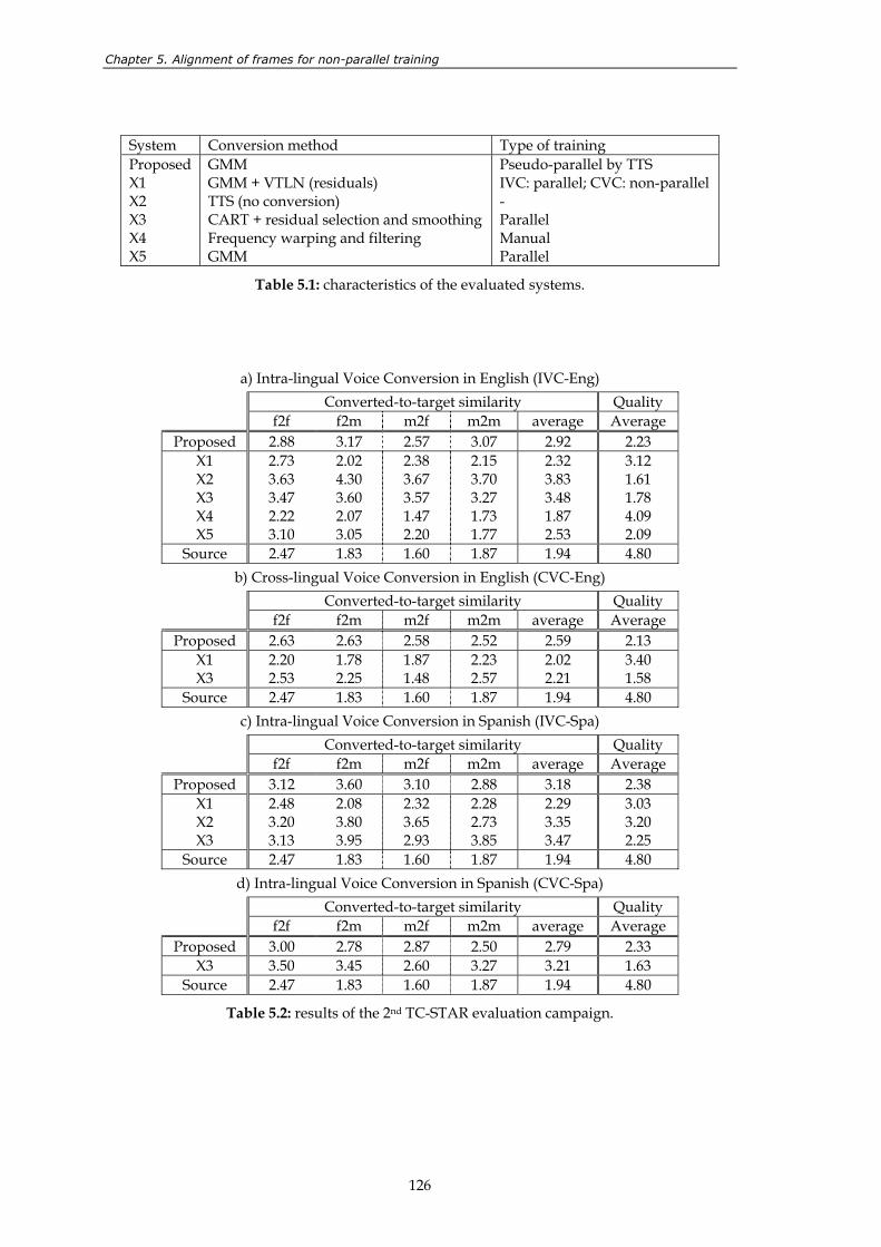
Chapter 5. Alignment of frames for non-parallel training
126
System Conversion method Type of training Proposed X1 X2 X3 X4 X5
GMM GMM + VTLN (residuals) TTS (no conversion) CART + residual selection and smoothing Frequency warping and filtering GMM
Pseudo-parallel by TTS IVC: parallel; CVC: non-parallel - Parallel Manual Parallel
Table 5.1: characteristics of the evaluated systems.
a) Intra-lingual Voice Conversion in English (IVC-Eng) Converted-to-target similarity Quality
f2f f2m m2f m2m average Average Proposed 2.88 3.17 2.57 3.07 2.92 2.23
X1 X2 X3 X4 X5
2.73 3.63 3.47 2.22 3.10
2.02 4.30 3.60 2.07 3.05
2.38 3.67 3.57 1.47 2.20
2.15 3.70 3.27 1.73 1.77
2.32 3.83 3.48 1.87 2.53
3.12 1.61 1.78 4.09 2.09
Source 2.47 1.83 1.60 1.87 1.94 4.80 b) Cross-lingual Voice Conversion in English (CVC-Eng)
Converted-to-target similarity Quality f2f f2m m2f m2m average Average
Proposed 2.63 2.63 2.58 2.52 2.59 2.13 X1 X3
2.20 2.53
1.78 2.25
1.87 1.48
2.23 2.57
2.02 2.21
3.40 1.58
Source 2.47 1.83 1.60 1.87 1.94 4.80 c) Intra-lingual Voice Conversion in Spanish (IVC-Spa)
Converted-to-target similarity Quality f2f f2m m2f m2m average Average
Proposed 3.12 3.60 3.10 2.88 3.18 2.38 X1 X2 X3
2.48 3.20 3.13
2.08 3.80 3.95
2.32 3.65 2.93
2.28 2.73 3.85
2.29 3.35 3.47
3.03 3.20 2.25
Source 2.47 1.83 1.60 1.87 1.94 4.80 d) Intra-lingual Voice Conversion in Spanish (CVC-Spa)
Converted-to-target similarity Quality f2f f2m m2f m2m average Average
Proposed 3.00 2.78 2.87 2.50 2.79 2.33 X3 3.50 3.45 2.60 3.27 3.21 1.63
Source 2.47 1.83 1.60 1.87 1.94 4.80
Table 5.2: results of the 2nd TC-STAR evaluation campaign.
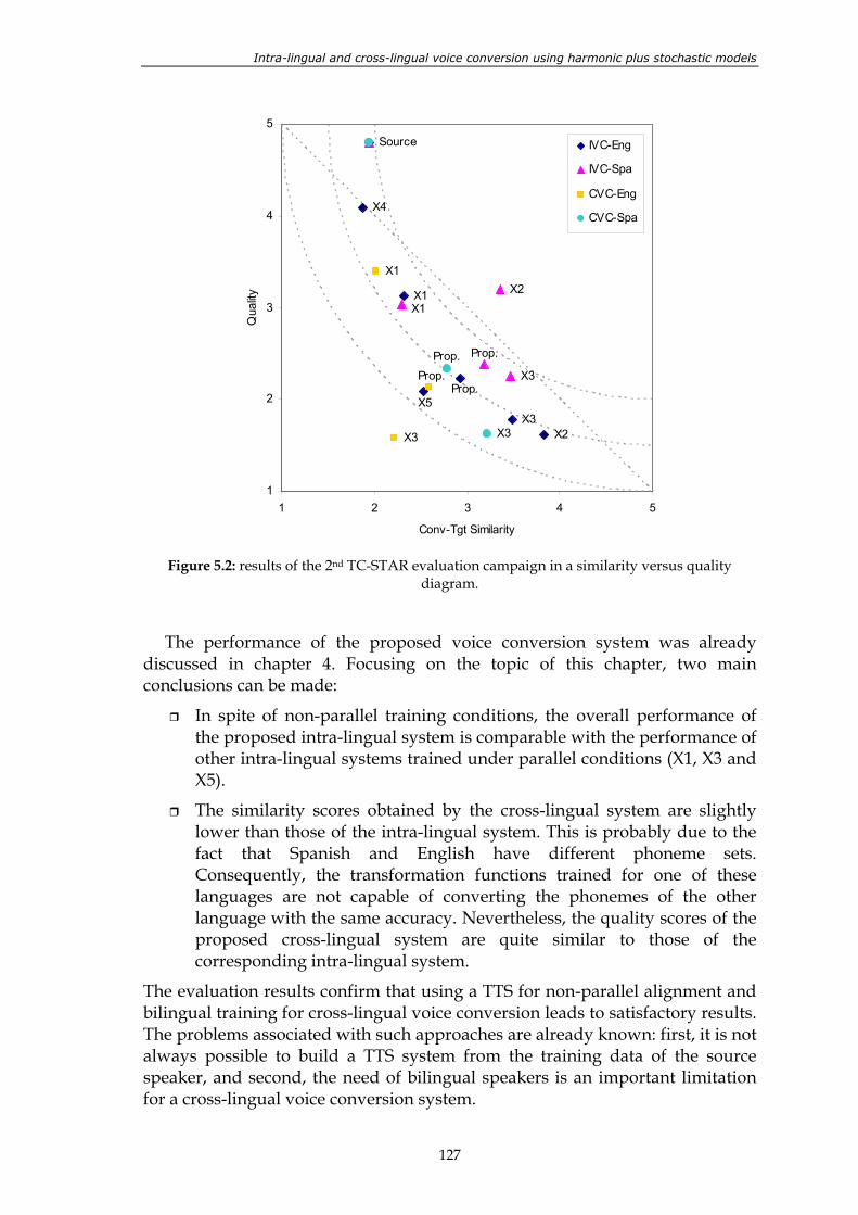
Intra-lingual and cross-lingual voice conversion using harmonic plus stochastic models
127
X2X3
X4
X5
X1
Prop.
X2
X3
Source
X1
Prop.
Prop.
X1
X3
Prop.
X3
1
2
3
4
5
1 2 3 4 5
Conv-Tgt Similarity
Qua
lity
IVC-Eng
IVC-Spa
CVC-Eng
CVC-Spa
Figure 5.2: results of the 2nd TC-STAR evaluation campaign in a similarity versus quality
diagram.
The performance of the proposed voice conversion system was already discussed in chapter 4. Focusing on the topic of this chapter, two main conclusions can be made:
In spite of non-parallel training conditions, the overall performance of the proposed intra-lingual system is comparable with the performance of other intra-lingual systems trained under parallel conditions (X1, X3 and X5).
The similarity scores obtained by the cross-lingual system are slightly lower than those of the intra-lingual system. This is probably due to the fact that Spanish and English have different phoneme sets. Consequently, the transformation functions trained for one of these languages are not capable of converting the phonemes of the other language with the same accuracy. Nevertheless, the quality scores of the proposed cross-lingual system are quite similar to those of the corresponding intra-lingual system.
The evaluation results confirm that using a TTS for non-parallel alignment and bilingual training for cross-lingual voice conversion leads to satisfactory results. The problems associated with such approaches are already known: first, it is not always possible to build a TTS system from the training data of the source speaker, and second, the need of bilingual speakers is an important limitation for a cross-lingual voice conversion system.
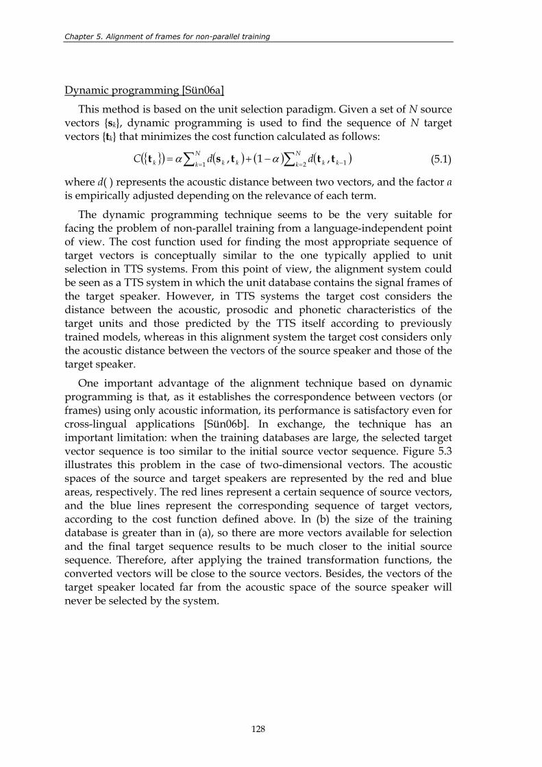
Chapter 5. Alignment of frames for non-parallel training
128
Dynamic programming [Sün06a]
This method is based on the unit selection paradigm. Given a set of N source vectors sk, dynamic programming is used to find the sequence of N target vectors tk that minimizes the cost function calculated as follows:
( ) ( ) ( ) ( )∑∑ = −=−+=
N
k kkN
k kkk ddC2 11
,1, tttst αα (5.1)
where d( ) represents the acoustic distance between two vectors, and the factor α is empirically adjusted depending on the relevance of each term.
The dynamic programming technique seems to be the very suitable for facing the problem of non-parallel training from a language-independent point of view. The cost function used for finding the most appropriate sequence of target vectors is conceptually similar to the one typically applied to unit selection in TTS systems. From this point of view, the alignment system could be seen as a TTS system in which the unit database contains the signal frames of the target speaker. However, in TTS systems the target cost considers the distance between the acoustic, prosodic and phonetic characteristics of the target units and those predicted by the TTS itself according to previously trained models, whereas in this alignment system the target cost considers only the acoustic distance between the vectors of the source speaker and those of the target speaker.
One important advantage of the alignment technique based on dynamic programming is that, as it establishes the correspondence between vectors (or frames) using only acoustic information, its performance is satisfactory even for cross-lingual applications [Sün06b]. In exchange, the technique has an important limitation: when the training databases are large, the selected target vector sequence is too similar to the initial source vector sequence. Figure 5.3 illustrates this problem in the case of two-dimensional vectors. The acoustic spaces of the source and target speakers are represented by the red and blue areas, respectively. The red lines represent a certain sequence of source vectors, and the blue lines represent the corresponding sequence of target vectors, according to the cost function defined above. In (b) the size of the training database is greater than in (a), so there are more vectors available for selection and the final target sequence results to be much closer to the initial source sequence. Therefore, after applying the trained transformation functions, the converted vectors will be close to the source vectors. Besides, the vectors of the target speaker located far from the acoustic space of the source speaker will never be selected by the system.
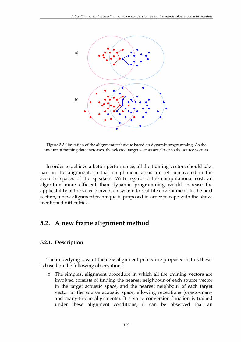
Intra-lingual and cross-lingual voice conversion using harmonic plus stochastic models
129
Figure 5.3: limitation of the alignment technique based on dynamic programming. As the
amount of training data increases, the selected target vectors are closer to the source vectors.
In order to achieve a better performance, all the training vectors should take part in the alignment, so that no phonetic areas are left uncovered in the acoustic spaces of the speakers. With regard to the computational cost, an algorithm more efficient than dynamic programming would increase the applicability of the voice conversion system to real-life environment. In the next section, a new alignment technique is proposed in order to cope with the above mentioned difficulties.
5.2. A new frame alignment method
5.2.1. Description
The underlying idea of the new alignment procedure proposed in this thesis is based on the following observations:
The simplest alignment procedure in which all the training vectors are involved consists of finding the nearest neighbour of each source vector in the target acoustic space, and the nearest neighbour of each target vector in the source acoustic space, allowing repetitions (one-to-many and many-to-one alignments). If a voice conversion function is trained under these alignment conditions, it can be observed that an
a)
b)
Chapter 5. Alignment of frames for non-parallel training
130
intermediate converted voice is obtained: it is different from the source voice but also different from the target voice. There is not enough similarity between the converted voice and the target voice to consider that the conversion is successful, but improvements could be expected if the source voice was substituted by the intermediate voice and the alignment was repeated.
If a linear voice conversion function based on GMMs is estimated from vector pairs aligned by nearest neighbour search, the over-smoothing helps to minimize the effect of misaligned vectors and one-to-many alignments. Although such an excessive smoothing was found to be problematic for voice conversion functions trained from parallel corpora, it is advantageous if the alignment between acoustic vectors is not perfect.
Figure 5.4: idea of the new alignment method.
Thus, the observations point to the hypothesis that an iterative refinement of the basic nearest neighbour method combined with voice conversion would lead to a progressive improvement in the alignment. The underlying idea is illustrated in figure 5.4: the intermediate voice obtained after the first nearest neighbour alignment can be used as the source voice during the next iteration. The process can be repeated until the current intermediate voice is close enough to the target voice. This algorithm can be formulated as follows. Let X=xk and Y=yj be the set of acoustic vectors of the source and target speaker, respectively. The new alignment algorithm consists of the following steps:
1. One more auxiliary vector set X’ is defined: X’=xk’. It is initialized as xk’=xk.
2. For each vector xk’ in X’, the index of its nearest neighbour in Y is found and stored as p(k). Similarly, the nearest neighbour of each vector yj is found in X’, and its index is stored as q(j).
3. An auxiliary GMM-based linear transformation function F is trained from the paired vectors xk, yp(k) and xq(j), yj. Note that the vectors used
Interm.
Source
Target Target Target Target
Interm.Interm.
Iter.0 Iter.1 Iter.2 Iter.3
Intra-lingual and cross-lingual voice conversion using harmonic plus stochastic models
131
to train the function F are always those belonging to X and Y, whereas the ones belonging to X’ are used only to refine the nearest neighbour alignment. Each vector in X is allowed to be paired with more than one vector in Y, and vice versa. Only the repeated pairs are eliminated. It is assumed that the continuous probabilistic function F smoothes the effect of the one-to-many or many-to-one alignments. The way of training the function F was already described in chapter 4: the paired vectors are concatenated together, and a joint GMM, given by the weights αi, the mean vectors µi and the covariance matrices Σi of the m gaussian components, is fitted to the resulting joint vector space by applying the EM algorithm (see section 4.2 for more details). The matrices and vectors necessary for the transformation can be extracted directly from the model parameters:
=
= yy
iyxi
xyi
xxi
iyi
xi
i ΣΣΣΣ
Σµµ
µ , (5.2)
( ) ( ) ( )[ ]∑ =
−−+=
m
ixi
xxi
yxi
yiipF
1
1 µxΣΣµxx (5.3)
where pi(x) denotes the probability of an acoustic source vector x to belong to the ith gaussian component of the model.
4. The auxiliary vector set X’ is updated according to the new transformation function F:
( ) kF kk ∀=′ ,xx (5.4)
5. Back to step 2 until convergence is reached.
The whole process is illustrated in figure 5.5 for a simple fictitious case of five two-dimensional vectors. Initially, the nearest neighbour alignment is not perfect, but some of the source vectors are paired with more than one target vector, and vice versa. When the first estimate of the auxiliary transformation function F is trained, the multiple alignments are smoothed and the source vector space is moved to an intermediate position. As the number of iterations increases, the alignment becomes more and more accurate. In figure 5.6, the algorithm is applied to align and convert two sets of two-dimensional vectors. The vectors were randomly generated according to the distributions with mean vectors equal to [0 0]T and [0 10]T, using unit covariance matrices. After 10 iterations, the converted source vectors are quite close to the target vectors. It is remarkable that the greatest improvements occur during the first iteration.
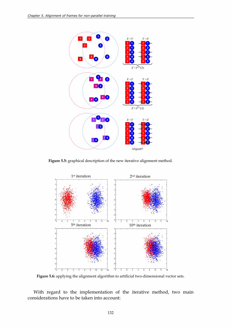
Chapter 5. Alignment of frames for non-parallel training
132
Figure 5.5: graphical description of the new iterative alignment method.
1st iteration
2nd iteration
5th iteration
10th iteration
Figure 5.6: applying the alignment algorithm to artificial two-dimensional vector sets.
With regard to the implementation of the iterative method, two main considerations have to be taken into account:
1 2
3
5 4
12
3
45
1
2
3
4
5
1
1
3
4
4
2
2
3
5
5
1
2
3
4
5
X→Y Y→X
1 2
3
5 4
12
3
45
1
2
3
4
5
1
1
3
4
5
2
2
3
4
5
1
2
3
4
5
X→Y Y→X
1 2
3
5 4
12
3
45
1
2
3
4
5
1
2
3
4
5
1
2
3
4
5
1
2
3
4
5
X→Y Y→X
Aligned!!
X’=F(0)(X)
X’=F(1)(X)
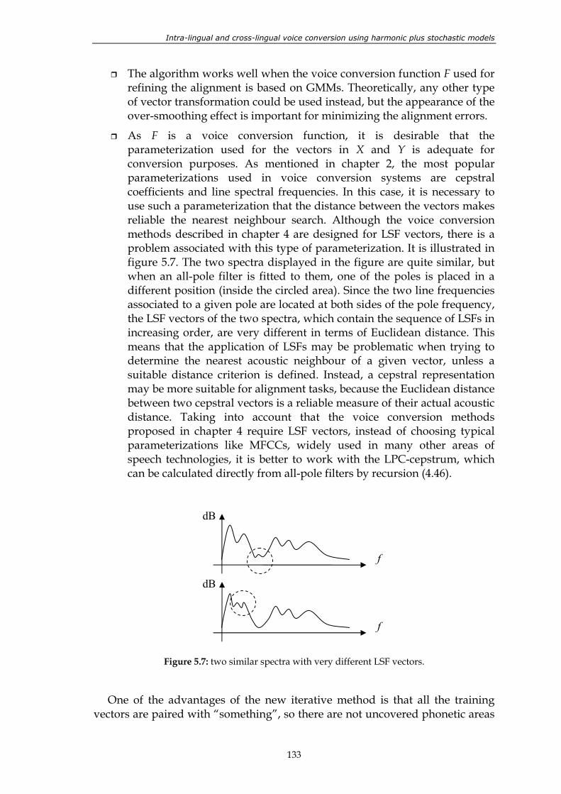
Intra-lingual and cross-lingual voice conversion using harmonic plus stochastic models
133
The algorithm works well when the voice conversion function F used for refining the alignment is based on GMMs. Theoretically, any other type of vector transformation could be used instead, but the appearance of the over-smoothing effect is important for minimizing the alignment errors.
As F is a voice conversion function, it is desirable that the parameterization used for the vectors in X and Y is adequate for conversion purposes. As mentioned in chapter 2, the most popular parameterizations used in voice conversion systems are cepstral coefficients and line spectral frequencies. In this case, it is necessary to use such a parameterization that the distance between the vectors makes reliable the nearest neighbour search. Although the voice conversion methods described in chapter 4 are designed for LSF vectors, there is a problem associated with this type of parameterization. It is illustrated in figure 5.7. The two spectra displayed in the figure are quite similar, but when an all-pole filter is fitted to them, one of the poles is placed in a different position (inside the circled area). Since the two line frequencies associated to a given pole are located at both sides of the pole frequency, the LSF vectors of the two spectra, which contain the sequence of LSFs in increasing order, are very different in terms of Euclidean distance. This means that the application of LSFs may be problematic when trying to determine the nearest acoustic neighbour of a given vector, unless a suitable distance criterion is defined. Instead, a cepstral representation may be more suitable for alignment tasks, because the Euclidean distance between two cepstral vectors is a reliable measure of their actual acoustic distance. Taking into account that the voice conversion methods proposed in chapter 4 require LSF vectors, instead of choosing typical parameterizations like MFCCs, widely used in many other areas of speech technologies, it is better to work with the LPC-cepstrum, which can be calculated directly from all-pole filters by recursion (4.46).
Figure 5.7: two similar spectra with very different LSF vectors.
One of the advantages of the new iterative method is that all the training vectors are paired with “something”, so there are not uncovered phonetic areas
f
f
dB
dB
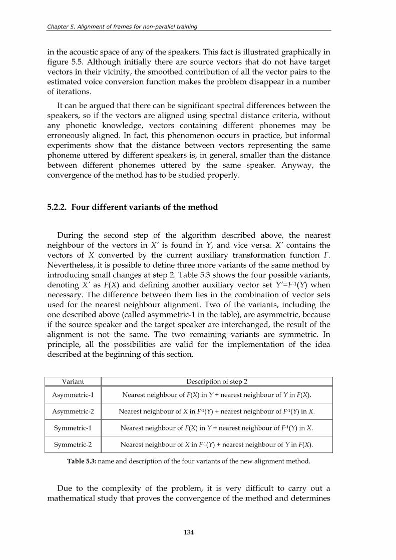
Chapter 5. Alignment of frames for non-parallel training
134
in the acoustic space of any of the speakers. This fact is illustrated graphically in figure 5.5. Although initially there are source vectors that do not have target vectors in their vicinity, the smoothed contribution of all the vector pairs to the estimated voice conversion function makes the problem disappear in a number of iterations.
It can be argued that there can be significant spectral differences between the speakers, so if the vectors are aligned using spectral distance criteria, without any phonetic knowledge, vectors containing different phonemes may be erroneously aligned. In fact, this phenomenon occurs in practice, but informal experiments show that the distance between vectors representing the same phoneme uttered by different speakers is, in general, smaller than the distance between different phonemes uttered by the same speaker. Anyway, the convergence of the method has to be studied properly.
5.2.2. Four different variants of the method
During the second step of the algorithm described above, the nearest neighbour of the vectors in X’ is found in Y, and vice versa. X’ contains the vectors of X converted by the current auxiliary transformation function F. Nevertheless, it is possible to define three more variants of the same method by introducing small changes at step 2. Table 5.3 shows the four possible variants, denoting X’ as F(X) and defining another auxiliary vector set Y’=F-1(Y) when necessary. The difference between them lies in the combination of vector sets used for the nearest neighbour alignment. Two of the variants, including the one described above (called asymmetric-1 in the table), are asymmetric, because if the source speaker and the target speaker are interchanged, the result of the alignment is not the same. The two remaining variants are symmetric. In principle, all the possibilities are valid for the implementation of the idea described at the beginning of this section.
Variant Description of step 2
Asymmetric-1 Nearest neighbour of F(X) in Y + nearest neighbour of Y in F(X).
Asymmetric-2 Nearest neighbour of X in F-1(Y) + nearest neighbour of F-1(Y) in X.
Symmetric-1 Nearest neighbour of F(X) in Y + nearest neighbour of F-1(Y) in X.
Symmetric-2 Nearest neighbour of X in F-1(Y) + nearest neighbour of Y in F(X).
Table 5.3: name and description of the four variants of the new alignment method.
Due to the complexity of the problem, it is very difficult to carry out a mathematical study that proves the convergence of the method and determines
Intra-lingual and cross-lingual voice conversion using harmonic plus stochastic models
135
the best variant of the algorithm. Instead, some objective experiments are conducted in order to prove that a true convergence occurs when the number of iterations is increased. The experimental conditions are the following:
Recordings from 4 different speakers are used: two male speakers (m1, m2) and two female speakers (f1, f2). Thus, 12 different conversion directions are possible.
For each conversion direction, 40 parallel sentences (approximately 2 minutes of audio) are used for training transformation functions based on 8th order GMMs (the experiment is based on objective measures, so GMM-based linear transformations are preferred above other methods characterized by lower objective scores like WFW). The fact that the sentences are parallel is ignored during the alignment process.
The order of the final transformation functions is fixed to 8, and the order of the auxiliary function F used for alignment purposes is one of the variables of the experiment (the over-smoothing effect, needed by the alignment system to work well, depends on the order of F). The number of iterations of the alignment method varies from 1 to 25 for all the variants of the method.
A set of 10 parallel sentences unseen during training is used for testing the accuracy of the trained functions by measuring the mean cepstral distance between the converted source vectors and their corresponding aligned target vectors, given by expression (4.31).
Figure 5.8 displays the mean distance values obtained by averaging the contribution of the 12 conversion directions for each of the variants of the method. From figure 5.8 we can observe that:
The four variants of the method provide lower mean distance scores when the number of iterations is increased, so in principle they point to convergence. Nevertheless, the discussion about the convergence will be taken up again in the next subsections.
Although there are slight differences between the 12 conversion directions, it can be seen that the variant called asymmetric-1 is clearly better than the rest. Therefore, the asymmetric-1 variant will be the one adopted in the experiments carried out from now on.
In average, the best results are obtained for an auxiliary transformation function of order 1, whose estimation is computationally less expensive and which produces stronger over-smoothing than higher-order functions. Considering only the asymmetric-1 variant, the individual scores obtained for each conversion direction, shown in the first column of figure 5.9, indicate that 1st order functions are not the best for all the conversion directions, but even when they are not, the distance scores provided by 1st order functions are very close to the lowest values.
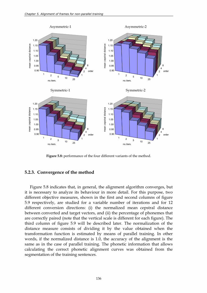
Chapter 5. Alignment of frames for non-parallel training
136
Asymmetric-1
1 2 5 10 25
12
48
0.90
0.95
1.00
1.05
1.10
1.15
1.20
mea
n ce
pstra
l dis
tanc
e
no.iters.
order
Asymmetric-2
1 2 5 10 25
12
48
0.90
0.95
1.00
1.05
1.10
1.15
1.20
mea
n ce
pstra
l dis
tanc
e
no.iters.
order
Symmetric-1
1 2 5 10 25
12
48
0.90
0.95
1.00
1.05
1.10
1.15
1.20
mea
n ce
pstra
l dis
tanc
e
no.iters.
order
Symmetric-2
1 2 5 10 25
12
48
0.90
0.95
1.00
1.05
1.10
1.15
1.20m
ean
ceps
tral d
ista
nce
no.iters.
order
Figure 5.8: performance of the four different variants of the method.
5.2.3. Convergence of the method
Figure 5.8 indicates that, in general, the alignment algorithm converges, but it is necessary to analyze its behaviour in more detail. For this purpose, two different objective measures, shown in the first and second columns of figure 5.9 respectively, are studied for a variable number of iterations and for 12 different conversion directions: (i) the normalized mean cepstral distance between converted and target vectors, and (ii) the percentage of phonemes that are correctly paired (note that the vertical scale is different for each figure). The third column of figure 5.9 will be described later. The normalization of the distance measure consists of dividing it by the value obtained when the transformation function is estimated by means of parallel training. In other words, if the normalized distance is 1.0, the accuracy of the alignment is the same as in the case of parallel training. The phonetic information that allows calculating the correct phonetic alignment curves was obtained from the segmentation of the training sentences.
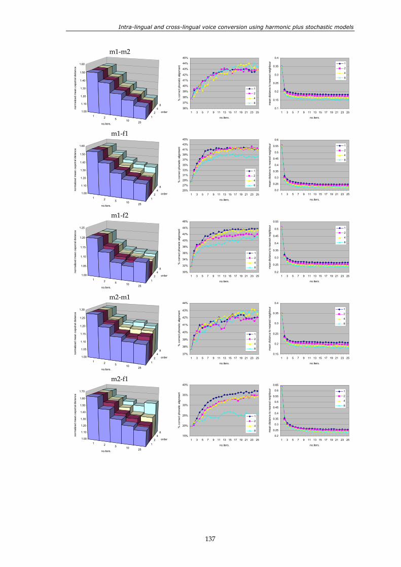
Intra-lingual and cross-lingual voice conversion using harmonic plus stochastic models
137
m1-m2
1 2 5 10 25
12
48
1.00
1.10
1.20
1.30
1.40
1.50
1.60
norm
aliz
ed m
ean
ceps
tral d
ista
nce
no.iters.
order
36%
37%
38%
39%
40%
41%
42%
43%
44%
45%
1 3 5 7 9 11 13 15 17 19 21 23 25
no.iters.
% c
orre
ct p
hone
tic a
lignm
ent
1
2
4
8
0.1
0.15
0.2
0.25
0.3
0.35
0.4
1 3 5 7 9 11 13 15 17 19 21 23 25
no.iters.
mea
n di
stan
ce to
nea
rest
nei
ghbo
ur 1
2
4
8
m1-f1
1 2 5 10 25
12
48
1.00
1.10
1.20
1.30
1.40
1.50
1.60
norm
aliz
ed m
ean
ceps
tral d
ista
nce
no.iters.
order
25%
27%
29%
31%
33%
35%
37%
39%
41%
43%
45%
1 3 5 7 9 11 13 15 17 19 21 23 25
no.iters.
% c
orre
ct p
hone
tic a
lignm
ent
1
2
4
8
0.2
0.25
0.3
0.35
0.4
0.45
0.5
0.55
0.6
1 3 5 7 9 11 13 15 17 19 21 23 25
no.iters.
mea
n di
stan
ce to
nea
rest
nei
ghbo
ur 1
2
4
8
m1-f2
1 2 5 10 25
12
48
1.00
1.05
1.10
1.15
1.20
1.25
norm
aliz
ed m
ean
ceps
tral d
ista
nce
no.iters.
order
30%
32%
34%
36%
38%
40%
42%
44%
46%
1 3 5 7 9 11 13 15 17 19 21 23 25
no.iters.
% c
orre
ct p
hone
tic a
lignm
ent
1
2
4
80.2
0.25
0.3
0.35
0.4
0.45
0.5
0.55
1 3 5 7 9 11 13 15 17 19 21 23 25
no.iters.
mea
n di
stan
ce to
nea
rest
nei
ghbo
ur 1
2
4
8
m2-m1
1 2 5 10 25
12
48
1.00
1.05
1.10
1.15
1.20
1.25
1.30
norm
aliz
ed m
ean
ceps
tral d
ista
nce
no.iters.
order
37%
38%
39%
40%
41%
42%
43%
44%
1 3 5 7 9 11 13 15 17 19 21 23 25
no.iters.
% c
orre
ct p
hone
tic a
lignm
ent
1
2
4
8
0.15
0.2
0.25
0.3
0.35
0.4
1 3 5 7 9 11 13 15 17 19 21 23 25
no.iters.
mea
n di
stan
ce to
nea
rest
nei
ghbo
ur 1
2
4
8
m2-f1
1 2 5 10 25
12
48
1.00
1.10
1.20
1.30
1.40
1.50
1.60
1.70
norm
aliz
ed m
ean
ceps
tral d
ista
nce
no.iters.
order
15%
20%
25%
30%
35%
40%
1 3 5 7 9 11 13 15 17 19 21 23 25
no.iters.
% c
orre
ct p
hone
tic a
lignm
ent
1
2
4
8
0.2
0.25
0.3
0.35
0.4
0.45
0.5
0.55
0.6
0.65
1 3 5 7 9 11 13 15 17 19 21 23 25
no.iters.
mea
n di
stan
ce to
nea
rest
nei
ghbo
ur 1
2
4
8
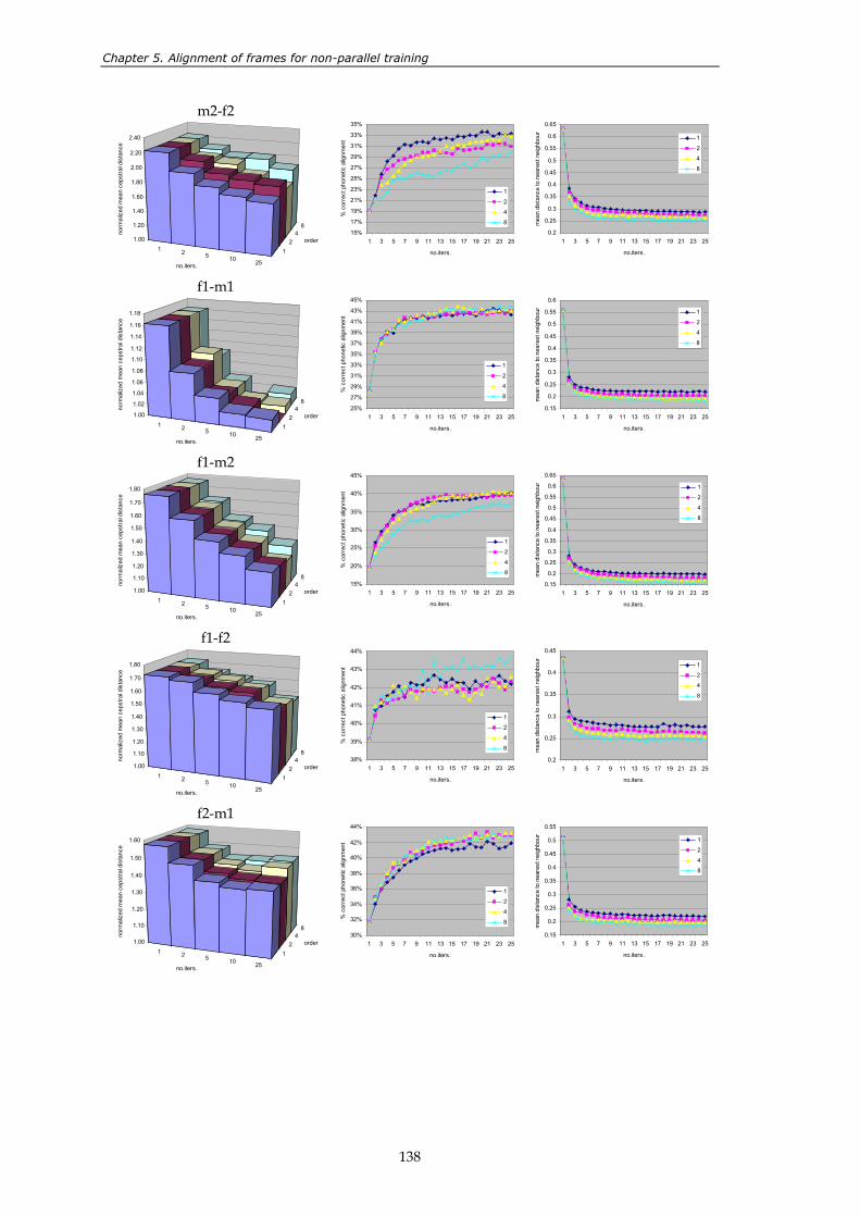
Chapter 5. Alignment of frames for non-parallel training
138
m2-f2
1 2 5 10 25
12
48
1.00
1.20
1.40
1.60
1.80
2.00
2.20
2.40
norm
aliz
ed m
ean
ceps
tral d
ista
nce
no.iters.
order
15%
17%
19%
21%
23%
25%
27%
29%
31%
33%
35%
1 3 5 7 9 11 13 15 17 19 21 23 25
no.iters.
% c
orre
ct p
hone
tic a
lignm
ent
1
2
4
8
0.2
0.25
0.3
0.35
0.4
0.45
0.5
0.55
0.6
0.65
1 3 5 7 9 11 13 15 17 19 21 23 25
no.iters.
mea
n di
stan
ce to
nea
rest
nei
ghbo
ur 1
2
4
8
f1-m1
1 2 5 10 25
12
48
1.00
1.02
1.04
1.06
1.08
1.10
1.12
1.14
1.16
1.18
norm
aliz
ed m
ean
ceps
tral d
ista
nce
no.iters.
order
25%
27%
29%
31%
33%
35%
37%
39%
41%
43%
45%
1 3 5 7 9 11 13 15 17 19 21 23 25
no.iters.
% c
orre
ct p
hone
tic a
lignm
ent
1
2
4
8
0.15
0.2
0.25
0.3
0.35
0.4
0.45
0.5
0.55
0.6
1 3 5 7 9 11 13 15 17 19 21 23 25
no.iters.
mea
n di
stan
ce to
nea
rest
nei
ghbo
ur 1
2
4
8
f1-m2
1 2 5 10 25
12
48
1.00
1.10
1.20
1.30
1.40
1.50
1.60
1.70
1.80
norm
aliz
ed m
ean
ceps
tral d
ista
nce
no.iters.
order
15%
20%
25%
30%
35%
40%
45%
1 3 5 7 9 11 13 15 17 19 21 23 25
no.iters.
% c
orre
ct p
hone
tic a
lignm
ent
1
2
4
8
0.15
0.2
0.25
0.3
0.35
0.4
0.45
0.5
0.55
0.6
0.65
1 3 5 7 9 11 13 15 17 19 21 23 25
no.iters.
mea
n di
stan
ce to
nea
rest
nei
ghbo
ur 1
2
4
8
f1-f2
1 2 5 10 25
12
48
1.00
1.10
1.20
1.30
1.40
1.50
1.60
1.70
1.80
norm
aliz
ed m
ean
ceps
tral d
ista
nce
no.iters.
order
38%
39%
40%
41%
42%
43%
44%
1 3 5 7 9 11 13 15 17 19 21 23 25
no.iters.
% c
orre
ct p
hone
tic a
lignm
ent
1
2
4
8
0.2
0.25
0.3
0.35
0.4
0.45
1 3 5 7 9 11 13 15 17 19 21 23 25
no.iters.
mea
n di
stan
ce to
nea
rest
nei
ghbo
ur 1
2
4
8
f2-m1
1 2 5 10 25
12
48
1.00
1.10
1.20
1.30
1.40
1.50
1.60
norm
aliz
ed m
ean
ceps
tral d
ista
nce
no.iters.
order
30%
32%
34%
36%
38%
40%
42%
44%
1 3 5 7 9 11 13 15 17 19 21 23 25
no.iters.
% c
orre
ct p
hone
tic a
lignm
ent
1
2
4
8
0.15
0.2
0.25
0.3
0.35
0.4
0.45
0.5
0.55
1 3 5 7 9 11 13 15 17 19 21 23 25
no.iters.
mea
n di
stan
ce to
nea
rest
nei
ghbo
ur 1
2
4
8
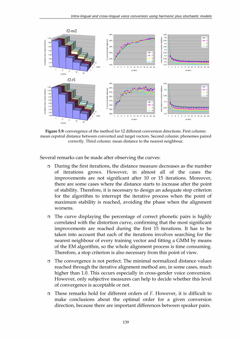
Intra-lingual and cross-lingual voice conversion using harmonic plus stochastic models
139
f2-m2
1 2 5 10 25
12
48
1.00
1.10
1.20
1.30
1.40
1.50
1.60
1.70
norm
aliz
ed m
ean
ceps
tral d
ista
nce
no.iters.
order
15%
20%
25%
30%
35%
40%
1 3 5 7 9 11 13 15 17 19 21 23 25
no.iters.
% c
orre
ct p
hone
tic a
lignm
ent
1
2
4
8
0.15
0.2
0.25
0.3
0.35
0.4
0.45
0.5
0.55
0.6
0.65
1 3 5 7 9 11 13 15 17 19 21 23 25
no.iters.
mea
n di
stan
ce to
nea
rest
nei
ghbo
ur 1
2
4
8
f2-f1
1 2 5 10 25
12
48
1.00
1.05
1.10
1.15
1.20
1.25
1.30
1.35
1.40
1.45
norm
aliz
ed m
ean
ceps
tral d
ista
nce
no.iters.
order
38%
39%
40%
41%
42%
43%
44%
45%
1 3 5 7 9 11 13 15 17 19 21 23 25
no.iters.
% c
orre
ct p
hone
tic a
lignm
ent
1
2
4
8
0.2
0.25
0.3
0.35
0.4
0.45
1 3 5 7 9 11 13 15 17 19 21 23 25
no.iters.
mea
n di
stan
ce to
nea
rest
nei
ghbo
ur 1
2
4
8
Figure 5.9: convergence of the method for 12 different conversion directions. First column: mean cepstral distance between converted and target vectors. Second column: phonemes paired
correctly. Third column: mean distance to the nearest neighbour.
Several remarks can be made after observing the curves:
During the first iterations, the distance measure decreases as the number of iterations grows. However, in almost all of the cases the improvements are not significant after 10 or 15 iterations. Moreover, there are some cases where the distance starts to increase after the point of stability. Therefore, it is necessary to design an adequate stop criterion for the algorithm to interrupt the iterative process when the point of maximum stability is reached, avoiding the phase when the alignment worsens.
The curve displaying the percentage of correct phonetic pairs is highly correlated with the distortion curve, confirming that the most significant improvements are reached during the first 15 iterations. It has to be taken into account that each of the iterations involves searching for the nearest neighbour of every training vector and fitting a GMM by means of the EM algorithm, so the whole alignment process is time consuming. Therefore, a stop criterion is also necessary from this point of view.
The convergence is not perfect. The minimal normalized distance values reached through the iterative alignment method are, in some cases, much higher than 1.0. This occurs especially in cross-gender voice conversion. However, only subjective measures can help to decide whether this level of convergence is acceptable or not.
These remarks hold for different orders of F. However, it is difficult to make conclusions about the optimal order for a given conversion direction, because there are important differences between speaker pairs.
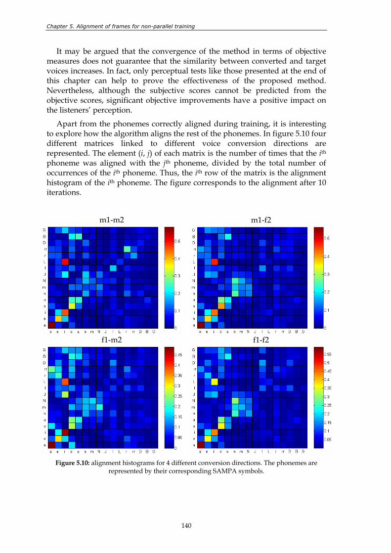
Chapter 5. Alignment of frames for non-parallel training
140
It may be argued that the convergence of the method in terms of objective measures does not guarantee that the similarity between converted and target voices increases. In fact, only perceptual tests like those presented at the end of this chapter can help to prove the effectiveness of the proposed method. Nevertheless, although the subjective scores cannot be predicted from the objective scores, significant objective improvements have a positive impact on the listeners’ perception.
Apart from the phonemes correctly aligned during training, it is interesting to explore how the algorithm aligns the rest of the phonemes. In figure 5.10 four different matrices linked to different voice conversion directions are represented. The element (i, j) of each matrix is the number of times that the ith phoneme was aligned with the jth phoneme, divided by the total number of occurrences of the ith phoneme. Thus, the ith row of the matrix is the alignment histogram of the ith phoneme. The figure corresponds to the alignment after 10 iterations.
m1-m2
m1-f2
f1-m2
f1-f2
Figure 5.10: alignment histograms for 4 different conversion directions. The phonemes are
represented by their corresponding SAMPA symbols.
Intra-lingual and cross-lingual voice conversion using harmonic plus stochastic models
141
Ideally, if all the phonemes were aligned correctly, identity matrices would be obtained. In practice, the matrices are not diagonal for several reasons:
The segmentation is not perfectly accurate, so some of the phonetic labels used for calculating the alignment histograms are incorrect and thus introduce small errors into the histograms. In fact, the presence of fricatives, plosives and other theoretically unvoiced phonemes among the voiced frames used for training is mainly due to segmentation inaccuracies. Since the number of frames belonging to such phonemes is too low to obtain statistically valid histograms for them, they were not included in the figure.
One phoneme may be often paired with a different phoneme because of coarticulation effects. For example, the Spanish phoneme /e/ is often paired with /i/ because, in certain coarticulation conditions, they are acoustically very similar. This phenomenon is not harmful for the performance of the system. The same happens to /u/ and /o/, /N/ and /n/, etc.
It can be concluded that, although the alignment is not perfect from a phonetic point of view, it is good from a spectral point of view.
5.2.4. Design of a stop criterion
The alignment method should stop iterating when there are no significant improvements from one iteration to the next one. Designing a stop condition means finding a variable that serves as the alignment accuracy indicator while the algorithm is running. Obviously, if the training corpus is non-parallel, it is not possible to measure objective distances like in the experiments above. Therefore, other solutions have to be explored. One possible strategy consists of measuring the similarity between the converted source vector space and the target vector space at the end of each iteration, and stopping the algorithm when they are close enough. Nevertheless, such a strategy requires an adequate modeling of the acoustic spaces at every iteration, and that is time consuming. That is why it is desirable to estimate the similarity between acoustic spaces directly from the training vectors. Using the notation from section 5.2.1, the idea proposed here consists of computing the distance between all the transformed source vectors in X’ and their nearest neighbour in Y, and vice versa, and then summing them together. The resulting global distance can be used for determining whether or not the current distance between X’ and Y is smaller than the previous one. The underlying idea is simple: the algorithm should stop when all the training vectors of one speaker are maximally close to the training vectors of the other speaker.
The third column of figure 5.9 shows the values of the mean nearest neighbour cepstral distance for 12 different voice conversion directions. 40 sentences were used for training. The number of alignment iterations was fixed
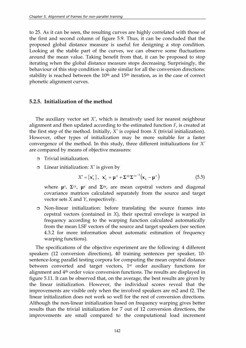
Chapter 5. Alignment of frames for non-parallel training
142
to 25. As it can be seen, the resulting curves are highly correlated with those of the first and second column of figure 5.9. Thus, it can be concluded that the proposed global distance measure is useful for designing a stop condition. Looking at the stable part of the curves, we can observe some fluctuations around the mean value. Taking benefit from that, it can be proposed to stop iterating when the global distance measure stops decreasing. Surprisingly, the behaviour of this stop condition is quite similar for all the conversion directions: stability is reached between the 10th and 15th iteration, as in the case of correct phonetic alignment curves.
5.2.5. Initialization of the method
The auxiliary vector set X’, which is iteratively used for nearest neighbour alignment and then updated according to the estimated function F, is created at the first step of the method. Initially, X’ is copied from X (trivial initialization). However, other types of initialization may be more suitable for a faster convergence of the method. In this study, three different initializations for X’ are compared by means of objective measures:
Trivial initialization.
Linear initialization: X’ is given by
( )xk
xxyyykkX µxΣΣµxx −+=′′=′
−1 , (5.5)
where µx, Σxx, µy and Σyy, are mean cepstral vectors and diagonal covariance matrices calculated separately from the source and target vector sets X and Y, respectively.
Non-linear initialization: before translating the source frames into cepstral vectors (contained in X), their spectral envelope is warped in frequency according to the warping function calculated automatically from the mean LSF vectors of the source and target speakers (see section 4.3.2 for more information about automatic estimation of frequency warping functions).
The specifications of the objective experiment are the following: 4 different speakers (12 conversion directions), 40 training sentences per speaker, 10-sentence-long parallel testing corpora for computing the mean cepstral distance between converted and target vectors, 1st order auxiliary functions for alignment and 4th order voice conversion functions. The results are displayed in figure 5.11. It can be observed that, on the average, the best results are given by the linear initialization. However, the individual scores reveal that the improvements are visible only when the involved speakers are m2 and f2. The linear initialization does not work so well for the rest of conversion directions. Although the non-linear initialization based on frequency warping gives better results than the trivial initialization for 7 out of 12 conversion directions, the improvements are small compared to the computational load increment
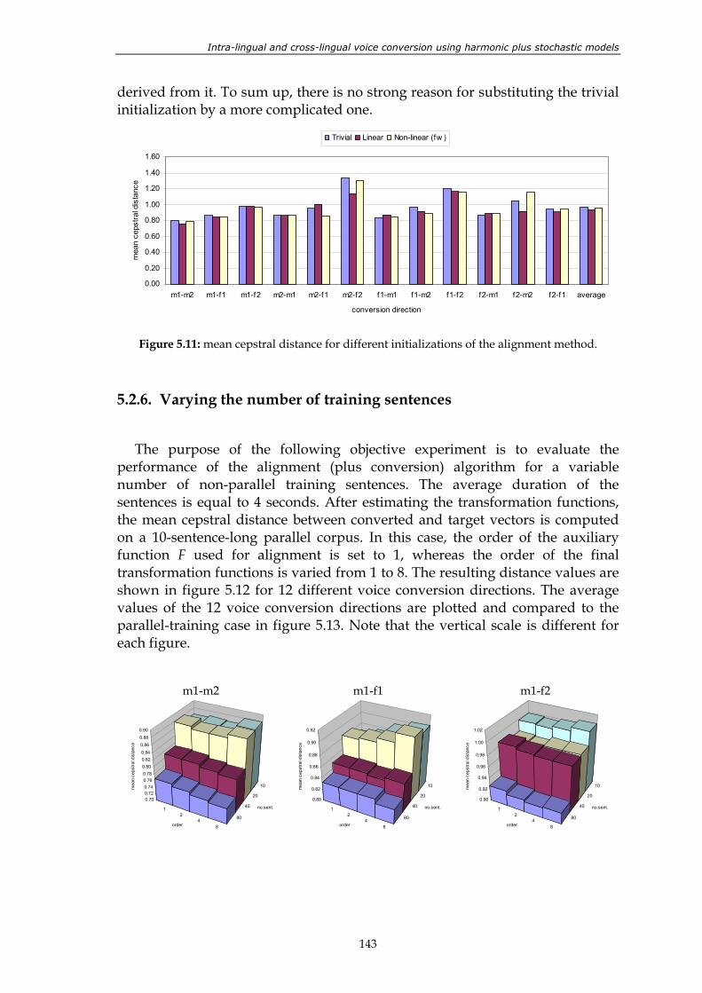
Intra-lingual and cross-lingual voice conversion using harmonic plus stochastic models
143
derived from it. To sum up, there is no strong reason for substituting the trivial initialization by a more complicated one.
0.00
0.20
0.40
0.60
0.80
1.00
1.20
1.40
1.60
m1-m2 m1-f1 m1-f2 m2-m1 m2-f1 m2-f2 f1-m1 f1-m2 f1-f2 f2-m1 f2-m2 f2-f1 average
conversion direction
mea
n ce
pstra
l dis
tanc
eTrivial Linear Non-linear (fw )
Figure 5.11: mean cepstral distance for different initializations of the alignment method.
5.2.6. Varying the number of training sentences
The purpose of the following objective experiment is to evaluate the performance of the alignment (plus conversion) algorithm for a variable number of non-parallel training sentences. The average duration of the sentences is equal to 4 seconds. After estimating the transformation functions, the mean cepstral distance between converted and target vectors is computed on a 10-sentence-long parallel corpus. In this case, the order of the auxiliary function F used for alignment is set to 1, whereas the order of the final transformation functions is varied from 1 to 8. The resulting distance values are shown in figure 5.12 for 12 different voice conversion directions. The average values of the 12 voice conversion directions are plotted and compared to the parallel-training case in figure 5.13. Note that the vertical scale is different for each figure.
m1-m2
12
48
80
40
20
10
0.700.720.740.760.780.800.820.840.860.880.90
mea
n ce
pstra
l dis
tanc
e
order
no.sent.
m1-f1
12
48
80
40
20
10
0.80
0.82
0.84
0.86
0.88
0.90
0.92
mea
n ce
pstra
l dis
tanc
e
order
no.sent.
m1-f2
12
48
80
40
20
10
0.90
0.92
0.94
0.96
0.98
1.00
1.02
mea
n ce
pstra
l dis
tanc
e
order
no.sent.
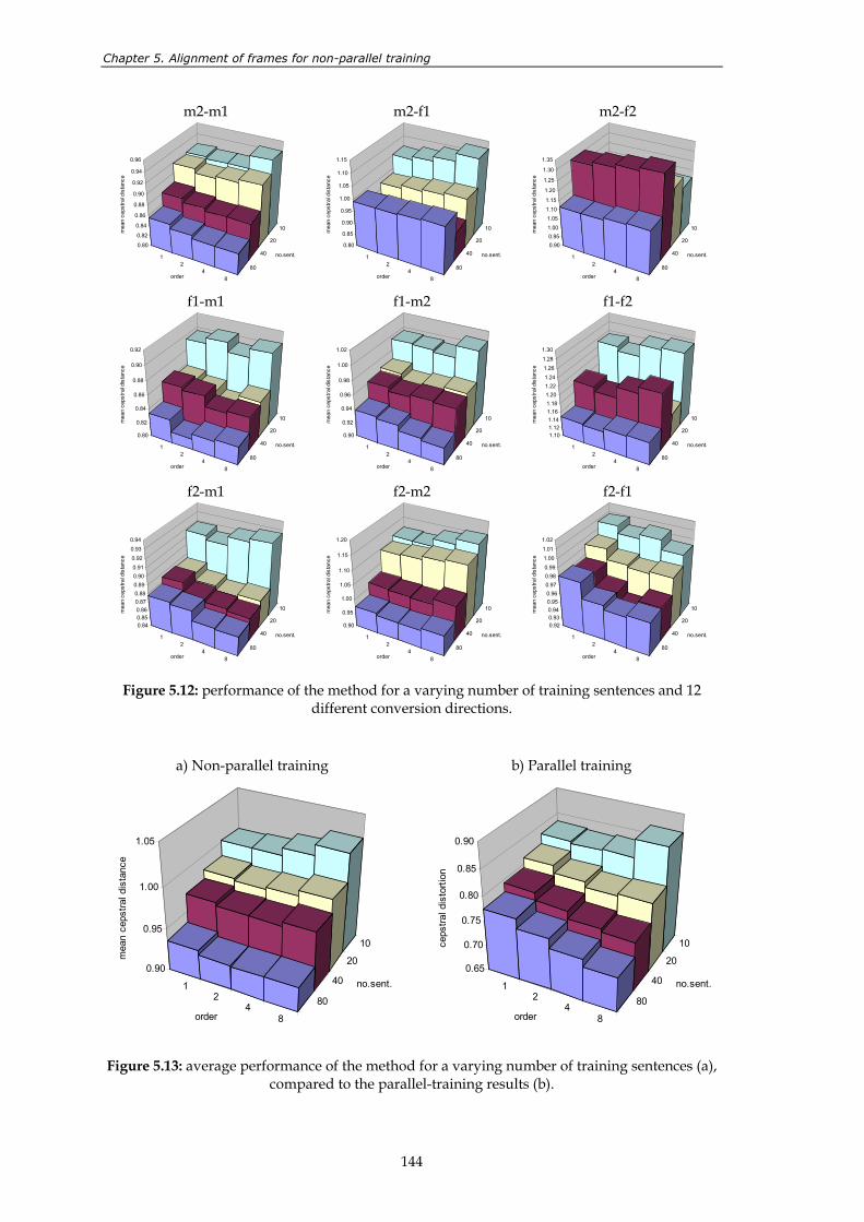
Chapter 5. Alignment of frames for non-parallel training
144
m2-m1
12
48
80
40
20
10
0.80
0.82
0.84
0.86
0.88
0.90
0.92
0.94
0.96
mea
n ce
pstra
l dis
tanc
e
order
no.sent.
m2-f1
12
48
80
40
20
10
0.80
0.85
0.90
0.95
1.00
1.05
1.10
1.15
mea
n ce
pstra
l dis
tanc
e
order
no.sent.
m2-f2
12
48
80
40
20
10
0.900.951.001.051.101.15
1.20
1.25
1.30
1.35
mea
n ce
pstra
l dis
tanc
e
order
no.sent.
f1-m1
12
48
80
40
20
10
0.80
0.82
0.84
0.86
0.88
0.90
0.92
mea
n ce
pstra
l dis
tanc
e
order
no.sent.
f1-m2
12
48
80
40
20
10
0.90
0.92
0.94
0.96
0.98
1.00
1.02
mea
n ce
pstra
l dis
tanc
e
order
no.sent.
f1-f2
12
48
80
40
20
10
1.101.121.141.161.181.201.221.241.261.281.30
mea
n ce
pstra
l dis
tanc
e
order
no.sent.
f2-m1
12
48
80
40
20
10
0.840.850.860.870.880.890.900.910.920.930.94
mea
n ce
pstra
l dis
tanc
e
order
no.sent.
f2-m2
12
48
80
40
20
10
0.90
0.95
1.00
1.05
1.10
1.15
1.20
mea
n ce
pstra
l dis
tanc
e
order
no.sent.
f2-f1
12
48
80
40
20
10
0.920.930.940.950.960.970.980.991.001.011.02
mea
n ce
pstra
l dis
tanc
e
order
no.sent.
Figure 5.12: performance of the method for a varying number of training sentences and 12 different conversion directions.
a) Non-parallel training
12
48
80
40
20
10
0.90
0.95
1.00
1.05
mea
n ce
pstra
l dis
tanc
e
order
no.sent.
b) Parallel training
12
48
80
40
20
10
0.65
0.70
0.75
0.80
0.85
0.90
ceps
tral d
isto
rtion
order
no.sent.
Figure 5.13: average performance of the method for a varying number of training sentences (a), compared to the parallel-training results (b).
Intra-lingual and cross-lingual voice conversion using harmonic plus stochastic models
145
The individual curves are more irregular than those obtained in chapter 4 for parallel training, since they are a consequence of combining the effects of over-smoothing, over-fitting, convergence of the iterative method and differences between speakers. In general, it can be observed that:
In almost all of the cases, the best results are obtained when the number of training sentences is maximal. On the average, the distance measure decreases when the number of training sentences is increased. The irregularities that can be observed individually for each conversion direction are probably due to the fact that the alignment algorithm is sensitive to the phonetic content of the training sentences.
In the non-parallel-training case, the order of the optimal transformation function for a given number of training sentences is always lower than in the parallel-training case. That is not surprising, because the over-smoothing effect is one of the reasons why the alignment algorithm works, and even when convergence is reached after a number of iterations, there are still some misalignments to be compensated by over-smoothing. Therefore, increasing the order of the transformation functions does not guarantee a more accurate conversion, even for a high number of training sentences. In general, 8th order transformation functions require at least 80 training sentences (around 5 minutes of audio).
5.2.7. Perceptual evaluation
Experiment 1
The alignment algorithm described along this chapter was integrated into a cross-lingual WFW-based voice conversion system that participated in the 3rd evaluation campaign of the European TC-STAR project. The evaluation conditions were the same as in the case of intra-lingual evaluation (section 4.3.3, experiment 2), except for the fact that the training sentences were cross-lingual.
The converted-to-target similarity and the quality of 2 converted sentences per system were rated by 20 listeners using a 1-to-5 MOS scale.
4 different conversion directions were considered again: male to male, male to female, female to male, and female to female.
All speakers were bilingual: for each speaker, around 150 Spanish sentences (source) or 150 English sentences (target) were available for training. The average duration of the sentences was around 3 or 4 seconds. 10 sentences unseen during the training process were used for the perceptual test.
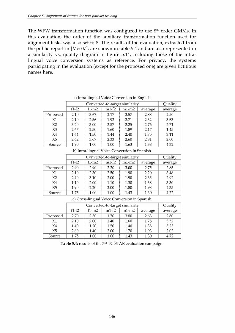
Chapter 5. Alignment of frames for non-parallel training
146
The WFW transformation function was configured to use 8th order GMMs. In this evaluation, the order of the auxiliary transformation function used for alignment tasks was also set to 8. The results of the evaluation, extracted from the public report in [Mos07], are shown in table 5.4 and are also represented in a similarity vs. quality diagram in figure 5.14, including those of the intra-lingual voice conversion systems as reference. For privacy, the systems participating in the evaluation (except for the proposed one) are given fictitious names here.
a) Intra-lingual Voice Conversion in English Converted-to-target similarity Quality
f1-f2 f1-m2 m1-f2 m1-m2 average average Proposed 2.10 3.67 2.17 3.57 2.88 2.50
X1 X2 X3 X4 X5
2.10 3.20 2.67 1.64 2.62
2.56 3.00 2.50 1.50 3.67
1.92 2.57 1.60 1.44 2.33
2.71 2.25 1.89 2.40 2.60
2.32 2.76 2.17 1.75 2.81
3.63 2.71 1.45 3.11 2.00
Source 1.90 1.00 1.00 1.63 1.38 4.32 b) Intra-lingual Voice Conversion in Spanish
Converted-to-target similarity Quality f1-f2 f1-m2 m1-f2 m1-m2 average average
Proposed 2.90 2.90 2.20 3.00 2.75 2.85 X1 X2 X4 X5
2.10 2.40 1.10 1.90
2.30 3.10 2.00 2.20
2.50 2.00 1.10 2.00
1.90 1.90 1.30 1.80
2.20 2.35 1.38 1.98
3.48 2.92 3.30 2.35
Source 1.75 1.00 1.00 1.43 1.30 4.72 c) Cross-lingual Voice Conversion in Spanish
Converted-to-target similarity Quality f1-f2 f1-m2 m1-f2 m1-m2 average average
Proposed 2.70 2.30 1.70 3.80 2.63 2.80 X1 X4 X5
2.10 1.40 2.60
2.00 1.20 1.40
1.40 1.50 2.00
1.60 1.40 1.70
1.78 1.38 1.93
3.52 3.23 2.02
Source 1.75 1.00 1.00 1.43 1.30 4.72
Table 5.4: results of the 3rd TC-STAR evaluation campaign.
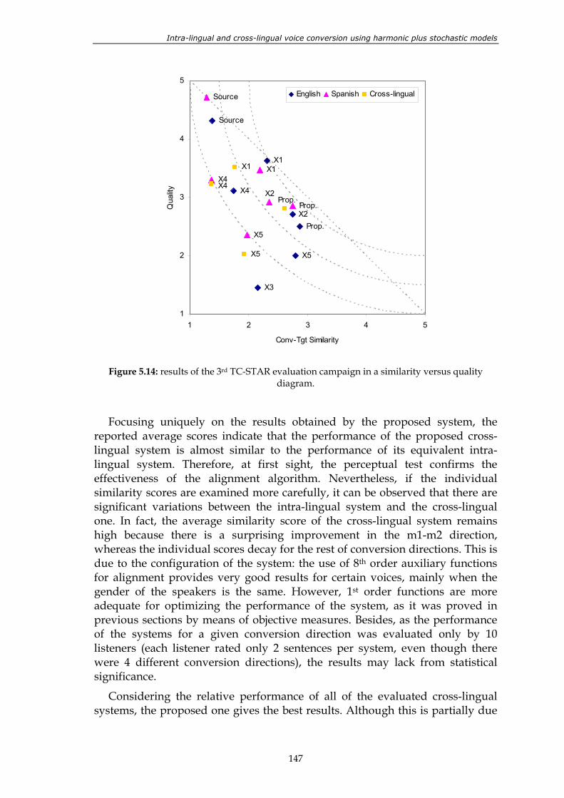
Intra-lingual and cross-lingual voice conversion using harmonic plus stochastic models
147
X2Prop.
X4
X5
X3
X1
Source
X4
X2Prop.
X5
X1
Source
Prop.
X1
X4
X5
1
2
3
4
5
1 2 3 4 5
Conv-Tgt Similarity
Qua
lity
English Spanish Cross-lingual
Figure 5.14: results of the 3rd TC-STAR evaluation campaign in a similarity versus quality
diagram.
Focusing uniquely on the results obtained by the proposed system, the reported average scores indicate that the performance of the proposed cross-lingual system is almost similar to the performance of its equivalent intra-lingual system. Therefore, at first sight, the perceptual test confirms the effectiveness of the alignment algorithm. Nevertheless, if the individual similarity scores are examined more carefully, it can be observed that there are significant variations between the intra-lingual system and the cross-lingual one. In fact, the average similarity score of the cross-lingual system remains high because there is a surprising improvement in the m1-m2 direction, whereas the individual scores decay for the rest of conversion directions. This is due to the configuration of the system: the use of 8th order auxiliary functions for alignment provides very good results for certain voices, mainly when the gender of the speakers is the same. However, 1st order functions are more adequate for optimizing the performance of the system, as it was proved in previous sections by means of objective measures. Besides, as the performance of the systems for a given conversion direction was evaluated only by 10 listeners (each listener rated only 2 sentences per system, even though there were 4 different conversion directions), the results may lack from statistical significance.
Considering the relative performance of all of the evaluated cross-lingual systems, the proposed one gives the best results. Although this is partially due
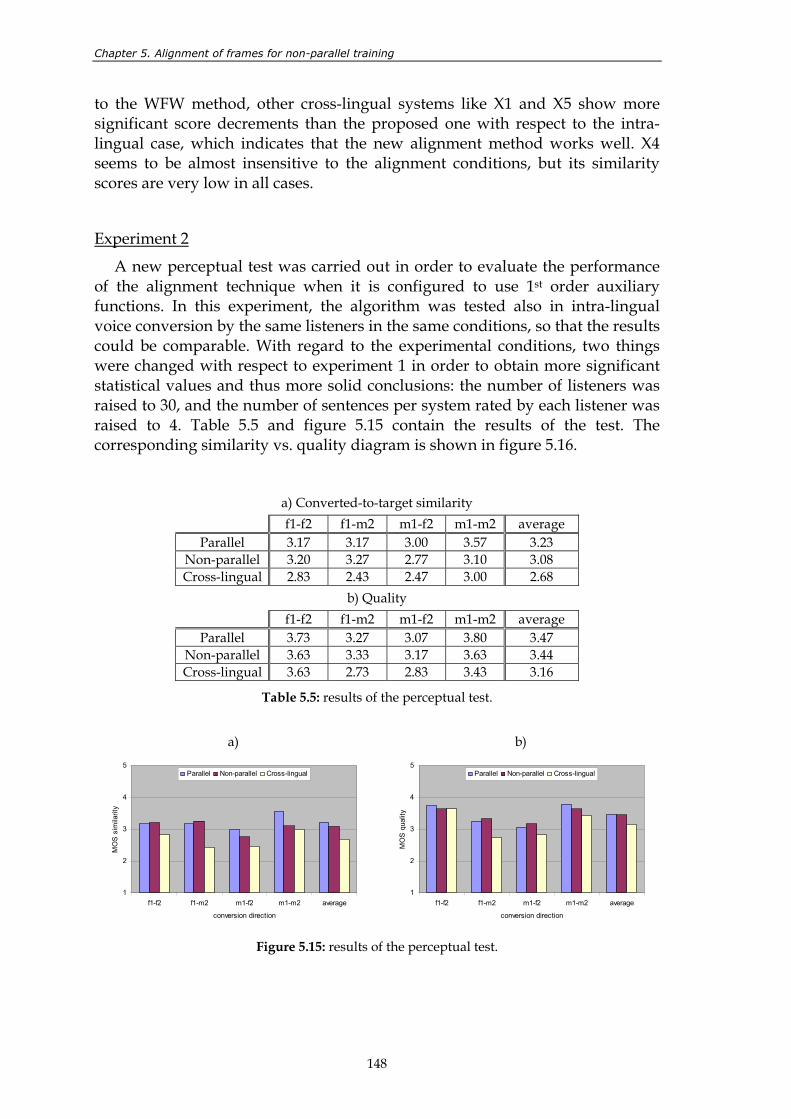
Chapter 5. Alignment of frames for non-parallel training
148
to the WFW method, other cross-lingual systems like X1 and X5 show more significant score decrements than the proposed one with respect to the intra-lingual case, which indicates that the new alignment method works well. X4 seems to be almost insensitive to the alignment conditions, but its similarity scores are very low in all cases.
Experiment 2
A new perceptual test was carried out in order to evaluate the performance of the alignment technique when it is configured to use 1st order auxiliary functions. In this experiment, the algorithm was tested also in intra-lingual voice conversion by the same listeners in the same conditions, so that the results could be comparable. With regard to the experimental conditions, two things were changed with respect to experiment 1 in order to obtain more significant statistical values and thus more solid conclusions: the number of listeners was raised to 30, and the number of sentences per system rated by each listener was raised to 4. Table 5.5 and figure 5.15 contain the results of the test. The corresponding similarity vs. quality diagram is shown in figure 5.16.
a) Converted-to-target similarity f1-f2 f1-m2 m1-f2 m1-m2 average
Parallel 3.17 3.17 3.00 3.57 3.23 Non-parallel 3.20 3.27 2.77 3.10 3.08 Cross-lingual 2.83 2.43 2.47 3.00 2.68
b) Quality f1-f2 f1-m2 m1-f2 m1-m2 average
Parallel 3.73 3.27 3.07 3.80 3.47 Non-parallel 3.63 3.33 3.17 3.63 3.44 Cross-lingual 3.63 2.73 2.83 3.43 3.16
Table 5.5: results of the perceptual test.
a)
1
2
3
4
5
f1-f2 f1-m2 m1-f2 m1-m2 average
conversion direction
MO
S s
imila
rity
Parallel Non-parallel Cross-lingual
b)
1
2
3
4
5
f1-f2 f1-m2 m1-f2 m1-m2 average
conversion direction
MO
S q
ualit
y
Parallel Non-parallel Cross-lingual
Figure 5.15: results of the perceptual test.
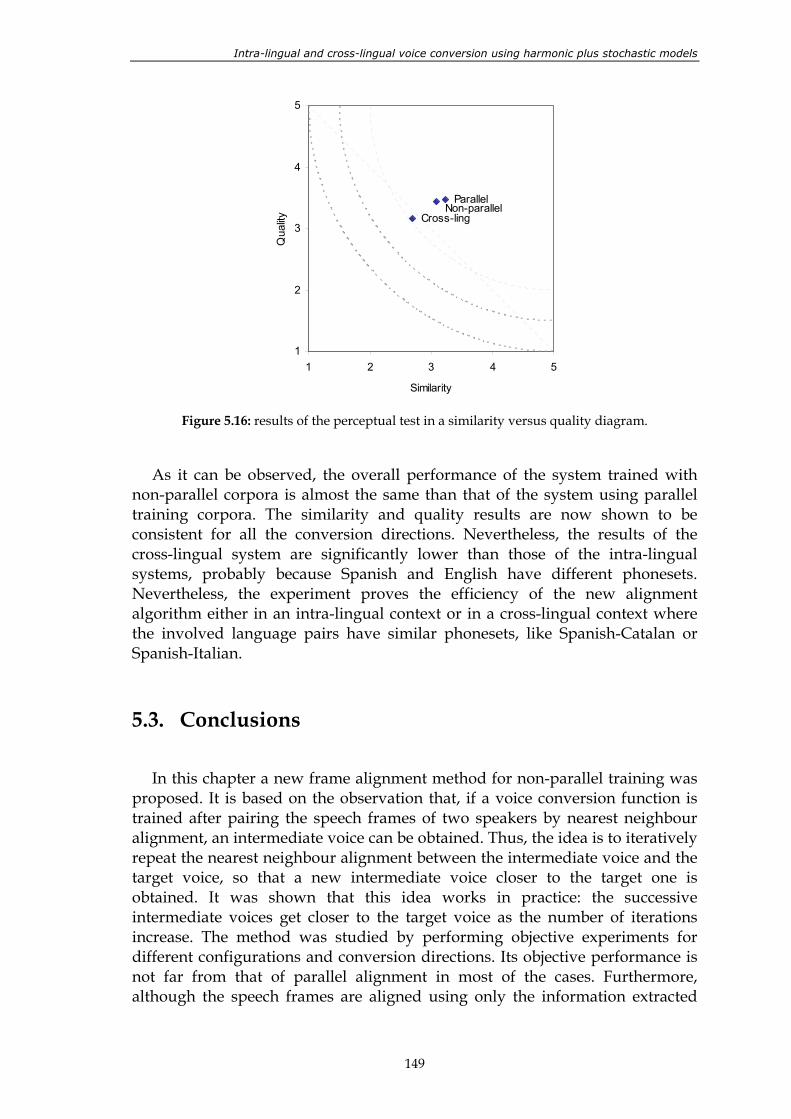
Intra-lingual and cross-lingual voice conversion using harmonic plus stochastic models
149
ParallelNon-parallel
Cross-ling
1
2
3
4
5
1 2 3 4 5
Similarity
Qua
lity
Figure 5.16: results of the perceptual test in a similarity versus quality diagram.
As it can be observed, the overall performance of the system trained with non-parallel corpora is almost the same than that of the system using parallel training corpora. The similarity and quality results are now shown to be consistent for all the conversion directions. Nevertheless, the results of the cross-lingual system are significantly lower than those of the intra-lingual systems, probably because Spanish and English have different phonesets. Nevertheless, the experiment proves the efficiency of the new alignment algorithm either in an intra-lingual context or in a cross-lingual context where the involved language pairs have similar phonesets, like Spanish-Catalan or Spanish-Italian.
5.3. Conclusions
In this chapter a new frame alignment method for non-parallel training was proposed. It is based on the observation that, if a voice conversion function is trained after pairing the speech frames of two speakers by nearest neighbour alignment, an intermediate voice can be obtained. Thus, the idea is to iteratively repeat the nearest neighbour alignment between the intermediate voice and the target voice, so that a new intermediate voice closer to the target one is obtained. It was shown that this idea works in practice: the successive intermediate voices get closer to the target voice as the number of iterations increase. The method was studied by performing objective experiments for different configurations and conversion directions. Its objective performance is not far from that of parallel alignment in most of the cases. Furthermore, although the speech frames are aligned using only the information extracted
Chapter 5. Alignment of frames for non-parallel training
150
directly from the signal, it was proved that the alignment is acceptable from a phonetic point of view. A stop criterion was designed for the system to decide automatically when the convergence is reached. Different types of initialization were also considered. Finally, it was demonstrated that, in contrast to other existing frame alignment methods, the proposed one gives better performance when the number of training sentences is increased.
The new alignment method was integrated into a cross-lingual voice conversion system based on WFW, which participated in one of the public evaluation campaigns organized in the framework of the European TC-STAR project. The results were excellent compared to the rest of the competitors, even though at the time of the evaluation the alignment method was not optimized yet.
Other carefully designed perceptual tests were carried out during the elaboration of this thesis. Their results indicate that, in an intra-lingual context, the performance of a WFW-based voice conversion system combined with the new alignment method is very good in absolute terms. In fact, the resulting scores are similar to those obtained by an equivalent voice conversion system trained on a parallel corpus. The scores worsen slightly when the system is trained in cross-lingual conditions, but the method is expected to be suitable for language pairs with similar phonesets.
Related publications
D. Erro, A. Moreno, “Frame Alignment Method for Cross-lingual Voice Conversion”, Interspeech 2007, Eurospeech. Antwerp, Belgium. August 2007.
151
6. Text-to-converted-speech synthesis
Until now, all the voice conversion methods and algorithms proposed in this thesis have been tested using natural speech recordings. Nevertheless, they can also be applied to converting synthetic speech. In fact, one of the main applications of voice conversion is customizing the voice of TTS systems, so this chapter is devoted to present new experiments in which a TTS system with a fixed synthesis unit database is asked to talk using different voices. In such an application, the resulting similarity scores should not differ from those obtained when converting natural utterances, whereas the quality of the converted signals is limited not only by the transformation method but also by the synthesis process itself.
At present, the two main types of systems that generate synthetic speech are based on unit selection and on hidden Markov models, respectively. The integration of voice conversion into a HMM-based synthesizer is quite easy and does not introduce complexity into the system: during the training phase, the acoustic models from which the system generates the output acoustic vectors are transformed by adaptation techniques. Thus, the synthesis-plus-conversion procedure is exactly the same than the pure synthesis procedure, as it has been explained in chapter 2. However, at the time of writing this thesis, TTS systems based on unit selection are still the best option in terms of quality and naturalness. That is the reason why unit selection synthesis is preferred for the experiments carried out in this chapter. In such systems, the integration of voice conversion into the waveform generation module requires paying some attention to how the synthesis and the conversion process interact. This topic is deeply analyzed in section 6.1. In section 6.2, a complete synthesis system with voice conversion is described and evaluated by listeners. Finally, in section 6.3 the conclusions of this part of the dissertation are summarized.
6.1. Integration of voice conversion into a synthesizer
In principle, the synthetic speech signals are also valid for being analyzed, converted and reconstructed in the same manner than natural recorded signals. A non-interactive combination between speech synthesis and voice conversion should provide results that depend on the individual performance of each block. The non-interactive converted-speech synthesis system is schematized in
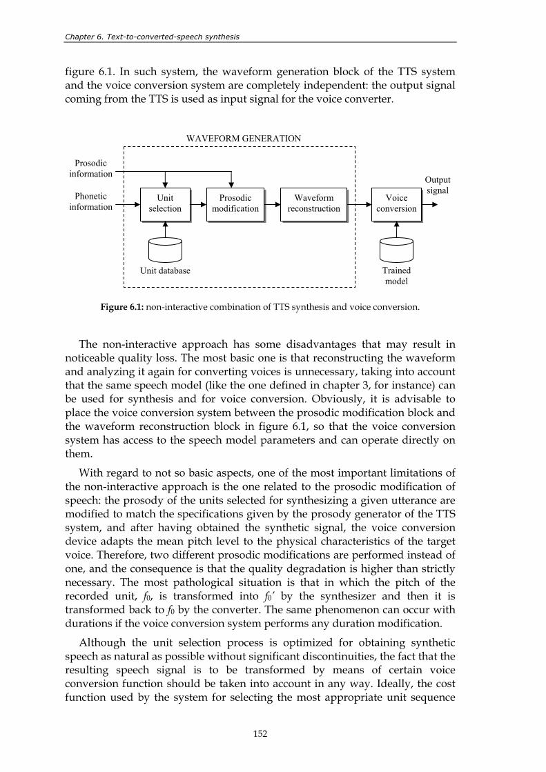
Chapter 6. Text-to-converted-speech synthesis
152
figure 6.1. In such system, the waveform generation block of the TTS system and the voice conversion system are completely independent: the output signal coming from the TTS is used as input signal for the voice converter.
Figure 6.1: non-interactive combination of TTS synthesis and voice conversion.
The non-interactive approach has some disadvantages that may result in noticeable quality loss. The most basic one is that reconstructing the waveform and analyzing it again for converting voices is unnecessary, taking into account that the same speech model (like the one defined in chapter 3, for instance) can be used for synthesis and for voice conversion. Obviously, it is advisable to place the voice conversion system between the prosodic modification block and the waveform reconstruction block in figure 6.1, so that the voice conversion system has access to the speech model parameters and can operate directly on them.
With regard to not so basic aspects, one of the most important limitations of the non-interactive approach is the one related to the prosodic modification of speech: the prosody of the units selected for synthesizing a given utterance are modified to match the specifications given by the prosody generator of the TTS system, and after having obtained the synthetic signal, the voice conversion device adapts the mean pitch level to the physical characteristics of the target voice. Therefore, two different prosodic modifications are performed instead of one, and the consequence is that the quality degradation is higher than strictly necessary. The most pathological situation is that in which the pitch of the recorded unit, f0, is transformed into f0’ by the synthesizer and then it is transformed back to f0 by the converter. The same phenomenon can occur with durations if the voice conversion system performs any duration modification.
Although the unit selection process is optimized for obtaining synthetic speech as natural as possible without significant discontinuities, the fact that the resulting speech signal is to be transformed by means of certain voice conversion function should be taken into account in any way. Ideally, the cost function used by the system for selecting the most appropriate unit sequence
Unit selection
Prosodic modification
Waveform reconstruction
Voice conversion
Phonetic information
Prosodic information
Unit database Trained model
WAVEFORM GENERATION
Output signal
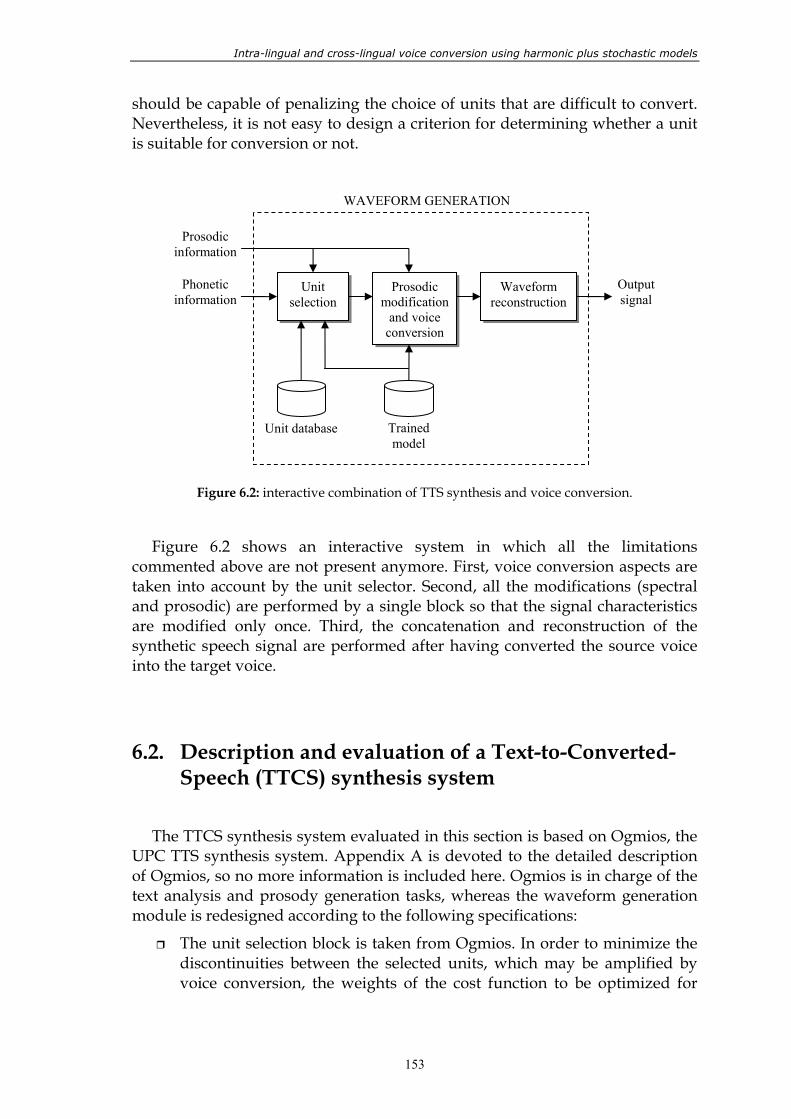
Intra-lingual and cross-lingual voice conversion using harmonic plus stochastic models
153
should be capable of penalizing the choice of units that are difficult to convert. Nevertheless, it is not easy to design a criterion for determining whether a unit is suitable for conversion or not.
Figure 6.2: interactive combination of TTS synthesis and voice conversion.
Figure 6.2 shows an interactive system in which all the limitations commented above are not present anymore. First, voice conversion aspects are taken into account by the unit selector. Second, all the modifications (spectral and prosodic) are performed by a single block so that the signal characteristics are modified only once. Third, the concatenation and reconstruction of the synthetic speech signal are performed after having converted the source voice into the target voice.
6.2. Description and evaluation of a Text-to-Converted-Speech (TTCS) synthesis system
The TTCS synthesis system evaluated in this section is based on Ogmios, the UPC TTS synthesis system. Appendix A is devoted to the detailed description of Ogmios, so no more information is included here. Ogmios is in charge of the text analysis and prosody generation tasks, whereas the waveform generation module is redesigned according to the following specifications:
The unit selection block is taken from Ogmios. In order to minimize the discontinuities between the selected units, which may be amplified by voice conversion, the weights of the cost function to be optimized for
Unit selection
Prosodic modification
and voice conversion
Waveform reconstruction
Phonetic information
Prosodic information
Unit database Trained model
WAVEFORM GENERATION
Output signal
Chapter 6. Text-to-converted-speech synthesis
154
selecting the most adequate unit sequence are adjusted so that the concatenation cost takes priority over the target cost.
The synthesis databases used for unit selection contain around 10 hours of audio. Two Ogmios voices are available: one female voice and one male voice. From now on, they will be called F and M, respectively.
The model chosen for reconstructing and modifying the prosody and the spectrum of the speech waveforms is the HSM presented in chapter 3. If the objective of the system was to obtain natural-sounding synthetic speech, the signal modification should be as little as possible. In this case, since the distortion introduced by prosodic manipulation is much lower than that introduced by voice conversion (including mean pitch level adaptation), the pitch contour of the selected unit sequence is forced to match exactly the specifications provided by the prosody generation block. The durations are modified only when the required factors are greater than a phoneme-dependent threshold (this strategy is usually applied by Ogmios).
A voice conversion system based on WFW is integrated into the waveform generator following an interactive scheme (figure 6.2). Nevertheless, it has to be clarified that no voice conversion constraints are taking into account by the unit selector.
For evaluating the performance of the TTCS system, several Spanish sentences were generated trying to imitate 4 different voices: f1, f2, m1 and m2, which are described in appendix B and have been already used in previous chapters. The transformation functions were estimated using parallel corpora built from around 150 sentences (the average duration of the sentences is 4 seconds). After some informal trials, it was observed that there were significant differences in the behaviour of F and M: F showed a very good behaviour in terms of WFW-based voice conversion, whereas M provided better synthetic speech than F but it was found to be more difficult to convert. For this reason, F was selected to be the basis voice of the system. 30 listeners were asked to rate the similarity between the converted-target sentence pairs (converted synthetic sentences versus natural speech recordings), and also the overall quality of the converted sentences, using a 5-point scale (in which the best score is 5).
Figure 6.3 shows the results of the perceptual evaluation. Apart from the average scores for each conversion direction and the total average scores (denoted as “avg”), the results of comparing the non-converted synthetic voice of the system with natural utterances of the same voice are also included (denoted as “self”). Such are helpful for determining how the synthesis process affects the similarity between voices and the quality of the signals.
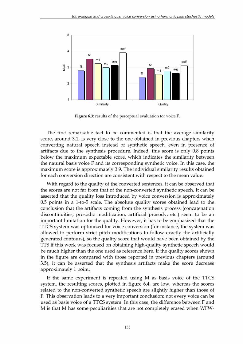
Intra-lingual and cross-lingual voice conversion using harmonic plus stochastic models
155
f1
f1
f2
f2m1
m1
m2m2
avg
avg
self
self
1
2
3
4
5
Similarity Quality
MO
S
Figure 6.3: results of the perceptual evaluation for voice F.
The first remarkable fact to be commented is that the average similarity score, around 3.1, is very close to the one obtained in previous chapters when converting natural speech instead of synthetic speech, even in presence of artifacts due to the synthesis procedure. Indeed, this score is only 0.8 points below the maximum expectable score, which indicates the similarity between the natural basis voice F and its corresponding synthetic voice. In this case, the maximum score is approximately 3.9. The individual similarity results obtained for each conversion direction are consistent with respect to the mean value.
With regard to the quality of the converted sentences, it can be observed that the scores are not far from that of the non-converted synthetic speech. It can be asserted that the quality loss introduced by voice conversion is approximately 0.5 points in a 1-to-5 scale. The absolute quality scores obtained lead to the conclusion that the artifacts coming from the synthesis process (concatenation discontinuities, prosodic modification, artificial prosody, etc.) seem to be an important limitation for the quality. However, it has to be emphasized that the TTCS system was optimized for voice conversion (for instance, the system was allowed to perform strict pitch modifications to follow exactly the artificially generated contours), so the quality score that would have been obtained by the TTS if this work was focused on obtaining high-quality synthetic speech would be much higher than the one used as reference here. If the quality scores shown in the figure are compared with those reported in previous chapters (around 3.5), it can be asserted that the synthesis artifacts make the score decrease approximately 1 point.
If the same experiment is repeated using M as basis voice of the TTCS system, the resulting scores, plotted in figure 6.4, are low, whereas the scores related to the non-converted synthetic speech are slightly higher than those of F. This observation leads to a very important conclusion: not every voice can be used as basis voice of a TTCS system. In this case, the difference between F and M is that M has some peculiarities that are not completely erased when WFW-
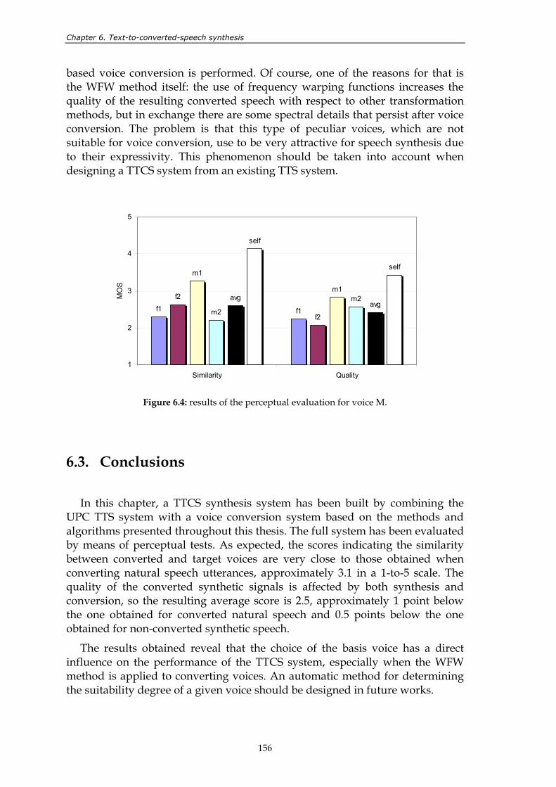
Chapter 6. Text-to-converted-speech synthesis
156
based voice conversion is performed. Of course, one of the reasons for that is the WFW method itself: the use of frequency warping functions increases the quality of the resulting converted speech with respect to other transformation methods, but in exchange there are some spectral details that persist after voice conversion. The problem is that this type of peculiar voices, which are not suitable for voice conversion, use to be very attractive for speech synthesis due to their expressivity. This phenomenon should be taken into account when designing a TTCS system from an existing TTS system.
f1 f1
f2
f2
m1
m1
m2
m2avgavg
self
self
1
2
3
4
5
Similarity Quality
MO
S
Figure 6.4: results of the perceptual evaluation for voice M.
6.3. Conclusions
In this chapter, a TTCS synthesis system has been built by combining the UPC TTS system with a voice conversion system based on the methods and algorithms presented throughout this thesis. The full system has been evaluated by means of perceptual tests. As expected, the scores indicating the similarity between converted and target voices are very close to those obtained when converting natural speech utterances, approximately 3.1 in a 1-to-5 scale. The quality of the converted synthetic signals is affected by both synthesis and conversion, so the resulting average score is 2.5, approximately 1 point below the one obtained for converted natural speech and 0.5 points below the one obtained for non-converted synthetic speech.
The results obtained reveal that the choice of the basis voice has a direct influence on the performance of the TTCS system, especially when the WFW method is applied to converting voices. An automatic method for determining the suitability degree of a given voice should be designed in future works.
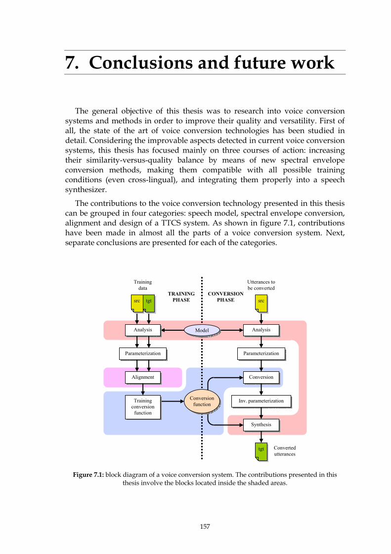
157
7. Conclusions and future work
The general objective of this thesis was to research into voice conversion systems and methods in order to improve their quality and versatility. First of all, the state of the art of voice conversion technologies has been studied in detail. Considering the improvable aspects detected in current voice conversion systems, this thesis has focused mainly on three courses of action: increasing their similarity-versus-quality balance by means of new spectral envelope conversion methods, making them compatible with all possible training conditions (even cross-lingual), and integrating them properly into a speech synthesizer.
The contributions to the voice conversion technology presented in this thesis can be grouped in four categories: speech model, spectral envelope conversion, alignment and design of a TTCS system. As shown in figure 7.1, contributions have been made in almost all the parts of a voice conversion system. Next, separate conclusions are presented for each of the categories.
Figure 7.1: block diagram of a voice conversion system. The contributions presented in this
thesis involve the blocks located inside the shaded areas.
Converted utterances
Analysis
Parameterization
Alignment
Training conversion
function
Analysis
Parameterization
Conversion
Synthesis
tgt
Inv. parameterization
TRAINING PHASE
CONVERSION PHASE src tgt
Training data
Utterances to be converted
src
Model
Conversion function
Chapter 7. Conclusions and future work
158
7.1. Harmonic plus stochastic model
In order to improve the analysis/synthesis part of the voice conversion system, a new speech model based on a harmonic plus stochastic decomposition has been presented in chapter 3. The harmonic component consists of a set of harmonically related sinusoids in the band 0-5KHz, given by their fundamental frequency, their amplitudes and their phases, whereas the stochastic component, which is assumed to occupy the full analysis band, is modelled by an all-pole filter estimated through LPC analysis. Novel algorithms for prosodic modification of speech signals, unit concatenation and phase envelope extraction have been also proposed. The main characteristic of such algorithms is that they are capable of operating on signals analyzed either at a constant or at a variable frame rate, so they provide a high degree of flexibility, even though they are based on conceptually quite simple ideas. The suitability of the new model and algorithms for speech synthesis under strong modification conditions (voice conversion implies strong modifications) has been proved by means of a comparison with TD-PSOLA.
Future work should be focused on the accuracy of the model. Since the objective in this first step of the thesis was building the analysis/synthesis part of a voice conversion system, the research has been focused on increasing the flexibility of the model, rather than on maximizing its accuracy. Therefore, although the model provides a good framework for speech analysis, modification and synthesis, there are several points where improvements can be made. The most remarkable one is the fact that the separation between the harmonic component and the stochastic component is not perfect. Any attempt of improving the harmonic-stochastic separation may benefit the model. Moreover, although the choice of a fixed value for the maximum voiced frequency is advantageous for spectral envelope extraction and thus for voice conversion, a more realistic model that allowed manipulating this parameter without losing voice conversion properties could be designed. In addition, a very simple method for synthesizing the stochastic component without considering its temporal structure has been used here, because the resulting quality is perceptually good, so an accurate modelling of the time behaviour of the noise-like part of the waveform would improve the quality of the reconstructed signals. However, the temporal parameters would have to be also transformed when converting voices.
7.2. Spectral envelope conversion
In chapter 4, the problem of increasing the quality of the converted speech without worsening the conversion performance has been faced. First, a baseline state-of-the-art system has been implemented. Then, a new spectral envelope conversion method called Weighted Frequency Warping has been proposed.
Intra-lingual and cross-lingual voice conversion using harmonic plus stochastic models
159
WFW is a combination between statistical transformation methods and frequency warping techniques. The training procedure of WFW consists of estimating a joint GMM from paired source-target acoustic vectors (like conventional GMM-based systems) and then calculating optimal frequency warping functions for each gaussian component of the model. During the conversion phase, these functions are combined to form a frame-dependent time-varying frequency warping function that is applied to the amplitude and phase envelopes, and after that, the energy distribution of the amplitude envelope is corrected using statistical linear transformations. The new spectral envelope conversion method results in much better quality scores than the baseline method (around 3.5 points in a 1-to-5 scale), whereas the conversion scores are kept almost invariant (around 3.0), so a good similarity-quality balance is achieved.
Future works addressed to improving WFW should start by studying certain voices that are not well converted by this method. For example, voices characterized (in a physical sense) by a low maximum voiced frequency (breathy voices, for instance) may be problematic when being transformed into other voices with higher maximum voiced frequency, because WFW extracts the original amplitude and phase envelopes from the harmonics detected between 0 and 5 KHz (the analysis procedure assumes that all the harmonics within this band exist, and forced detection is performed, so the amplitudes and phases detected above the physical maximum voiced frequency may not have true physical meaning), and then it calculates the target harmonics from the frequency-warped version of these envelopes. In order to extend WFW to expressive voices, the maximum voiced frequency should be included as a feature to be converted.
Furthermore, the combination between GMM-based statistical transformations and frequency warping transformations is made in the amplitude domain, whereas the phases are left unmodified after applying the frequency warping function to the original phase envelope. In principle, this does not have a noticeable negative impact on the quality of the resulting signals, but a solution should be proposed for keeping the amplitude and phase envelopes coherent.
7.3. Alignment for non-parallel training
A new frame alignment method has been also proposed in order to make the voice conversion system compatible with all possible training conditions, especially when a parallel training corpus is not available. The new method is based on using nearest neighbour alignment for obtaining an intermediate voice between the source and target voices, and then using the intermediate voice as source voice during the next iteration. After a number of iterations, the intermediate voice is close enough to the target voice. One of the main advantages of the method is that it does not require extra phonetic or linguistic
Chapter 7. Conclusions and future work
160
information for a correct performance, but only the same acoustic vectors used for voice conversion, so it is also compatible with cross-lingual applications. In an intra-lingual context, the performance of the whole alignment plus conversion method is similar to that of an equivalent system trained under ideal conditions, whereas in a cross-lingual context, the similarity and quality scores are slightly worse.
One of the aspects of the alignment method to be improved in a future work is the computational load: at each iteration, the system performs lots of nearest neighbour searches and then it estimates an adequate linear transformation from the paired vectors, so the overall process is time-consuming if the number of vectors is large. Apart from that, a way of improving the performance of the alignment system in cross-lingual conditions should be also investigated.
7.4. Text-to-converted-speech synthesis
A TTCS synthesis system has been built by combining Ogmios (the UPC TTS system) with a voice conversion system based on WFW. The similarity scores achieved by the system are very close to those obtained when converting natural speech utterances, around 3.1 in a 1-to-5 scale, whereas the quality scores, which are affected by both synthesis and conversion, are around 2.5, 1 point below the one obtained for converted natural speech and 0.5 points below the one obtained for non-converted synthetic speech.
The design of an automatic method for determining the suitability of a given voice for a TTCS system is proposed as future work. It has to be emphasized that the best option in terms of converted-speech synthesis may not coincide with the best option in terms of speech synthesis.
This thesis does not provide a method for including voice conversion constraints into the cost function of the unit selector of a TTS system. The performance of the system would be better if the cost function was redesigned to assign a higher selection probability to the units that the system is capable of converting well. This is one of the main challenges for future work.
All the methods and algorithms presented throughout this dissertation were designed to be text- and language-independent as possible. Nevertheless, when voice conversion is integrated into a TTS system, the phonetic information is available without an extra effort, so it is possible to configure the system so that only certain phonemes are converted while others are left unmodified or partially converted in order to preserve their quality. A carefully designed experimental procedure would help to determine the most relevant phonemes or phoneme groups for the similarity scores.
Intra-lingual and cross-lingual voice conversion using harmonic plus stochastic models
161
7.5. Merits derived from the thesis
7.5.1. Complete list of publications
D. Erro, T. Polyakova, A. Moreno, “On combining statistical methods and frequency warping for high-quality voice conversion”, accepted for publication in ICASSP 2008. Las Vegas, USA. March 2008.
Bonafonte, J. Adell, P. D. Agüero, D. Erro, I. Esquerra, A. Moreno, J. Pérez, T. Polyakova, “The UPC TTS System Description for the 2007 Blizzard Challenge”, 6th ISCA Workshop on Speech Synthesis. Bonn, Germany. August 2007.
D. Erro, A. Moreno, “Flexible Harmonic/Stochastic Speech Synthesis”, 6th ISCA Workshop on Speech Synthesis. Bonn, Germany. August 2007.
D. Erro, A. Moreno, “Frame Alignment Method for Cross-lingual Voice Conversion”, InterSpeech 2007 - EuroSpeech. Antwerp, Belgium. August 2007.
D. Erro, A. Moreno, “Weighted Frequency Warping for Voice Conversion”, InterSpeech 2007 - EuroSpeech. Antwerp, Belgium. August 2007.
Moreno, A. Bonafonte, J. Adell, P.D. Agüero, I. Esquerra, D. Erro, J. Pérez, T. Polyakova, H.U. Hain, J. Racky, D. Suendermann, I. Kiss, R. Fernández, Z. Shuang, “Deliverable D29. TTS: Progress Report”, technical report of the project TC-STAR (Technology and Corpora for Speech to Speech Translation). 2007.
D. Erro, A. Moreno, “Sistema de Síntesis Armónico/Estocástico en modo Pitch-Asíncrono aplicado a Conversión de Voz”, IV Jornadas en Tecnologías del Habla, IV JTH, Zaragoza, Spain. November 2006.
H. Duxans, D. Erro, J. Pérez, F. Diego, A. Bonafonte, A. Moreno, “Voice Conversion of Non-Aligned Data using Unit Selection”, TC-Star Workshop on Speech to Speech Translation. Barcelona, Spain. June 2006.
D. Erro, A. Moreno, “Efficient Speech Synthesis System using the Deterministic plus Stochastic Model”, 3rd International Conference on Speech Prosody 2006. Dresden, Germany. May 2006.
Bonafonte, H. Hoege, I. Kiss, A. Moreno, D. Suendermann, U. Ziegenhain, J. Adell, P. Aguero, H. Duxans, D. Erro, J. Nurminen, J. Perez, G. Strecha, M. Umbert, X. Wang, “Deliverable D9. TTS: Progress Report”, technical report of the project TC-STAR (Technology and Corpora for Speech to Speech Translation). May 2005.
D. Erro, A. Moreno, “A Pitch-Asynchronous Simple Method for Speech Synthesis by Diphone Concatenation using the Deterministic plus Stochastic
Chapter 7. Conclusions and future work
162
Model”, 10th International Conference on Speech and Computer, SPECOM 2005. Patras, Greece, pp. 321-324. October 2005.
7.5.2. Remarkable results in public evaluation campaigns
Albayzin06 Evaluation, IV Jornadas en Tecnologías del Habla, Zaragoza, Spain, 2006: winner in “speech synthesis” (imitating voices for cheating a biometric system). Evaluation report: D. Erro, A. Moreno, “Conversión de voz con muy pocos datos en evaluación automática”. More information: http://www.rthabla.es.
3rd Evaluation Campaign of the integrated European project TC-STAR, 2007: winner in cross-lingual voice conversion. More information: [Mos07].
163
Appendix A
Ogmios, the UPC text-to-speech synthesis system
Ogmios is the multilingual Text-to-Speech synthesis system created at the Universitat Politècnica de Catalunya [Bon06a, Bon07]. Ogmios was designed in such manner that the algorithms are to some extent language-independent, whereas language-dependencies are kept in the data as possible. In order to reduce the development cost, most of the techniques are either language-independent (e.g. acoustic modules) or data-driven (e.g. prosody generation, phonetic transcription). The system was originally developed in Catalan and Spanish, and later it was extended to other languages like French, Portuguese and English. The core of the system is a C++ set of modules with a common interface based on highly structured data describing linguistic relationships at different levels, ranging from a shallow description of the syntax until acoustic features of the speech segments to be concatenated.
Ogmios contains many modules, each one devoted to a specific function. They can be classified in three main areas: text analysis, prosody generation and waveform generation, as formally defined in [Per06].
Text analysis. First, it tokenises the input text and classifies each token (punctuation, acronyms, abbreviations, cardinal and ordinal numbers, time and data expressions, Internet locators, etc.) and they are expanded into full orthographic forms. The input to this module is plain text, which can be optionally marked with the SSML language. The text is labelled with part-of-speech tags using a statistical tagger. For Spanish, shallow parsing is also added. Finally, the pronunciation of words is obtained from a dictionary. A grapheme-to-phoneme converter predicts the pronunciation of unknown words, if necessary.
Prosody generator. This is the principal agent in obtaining natural sounding quality of synthetic speech. There are several tasks: phrasing, f0-contour generation, segmental duration assignment and intensity contour generation. Each of these tasks is performed by a single module.
Waveform generation. The synthesis is performed by concatenating recorded segments selected from a large database. The basic units are context-dependent semi-phones. Acoustic and phonological features are used to select the most appropriate sequence of segments. Phrase selection is introduced to get all the units from phrases which are completely present in the database, so that the requirements in terms of prosodic modification are minimized.
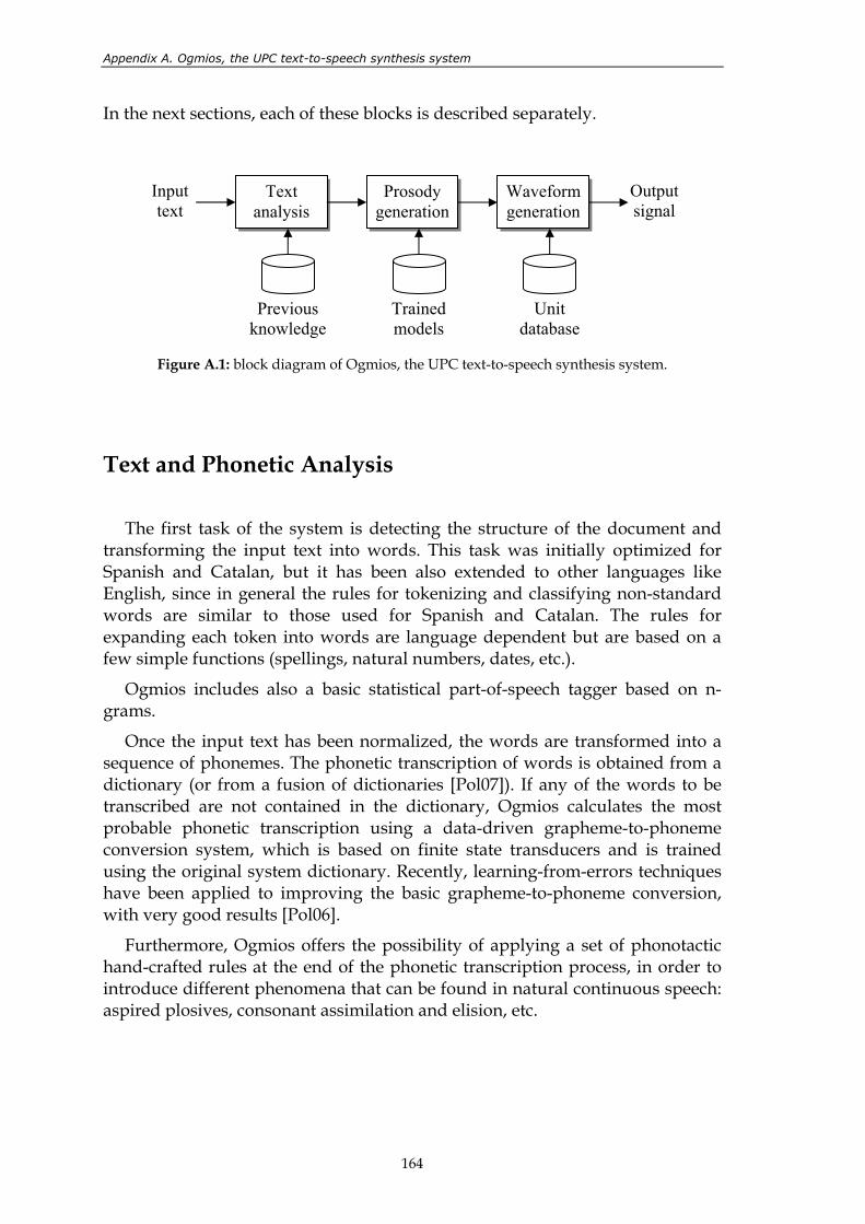
Appendix A. Ogmios, the UPC text-to-speech synthesis system
164
In the next sections, each of these blocks is described separately.
Figure A.1: block diagram of Ogmios, the UPC text-to-speech synthesis system.
Text and Phonetic Analysis
The first task of the system is detecting the structure of the document and transforming the input text into words. This task was initially optimized for Spanish and Catalan, but it has been also extended to other languages like English, since in general the rules for tokenizing and classifying non-standard words are similar to those used for Spanish and Catalan. The rules for expanding each token into words are language dependent but are based on a few simple functions (spellings, natural numbers, dates, etc.).
Ogmios includes also a basic statistical part-of-speech tagger based on n-grams.
Once the input text has been normalized, the words are transformed into a sequence of phonemes. The phonetic transcription of words is obtained from a dictionary (or from a fusion of dictionaries [Pol07]). If any of the words to be transcribed are not contained in the dictionary, Ogmios calculates the most probable phonetic transcription using a data-driven grapheme-to-phoneme conversion system, which is based on finite state transducers and is trained using the original system dictionary. Recently, learning-from-errors techniques have been applied to improving the basic grapheme-to-phoneme conversion, with very good results [Pol06].
Furthermore, Ogmios offers the possibility of applying a set of phonotactic hand-crafted rules at the end of the phonetic transcription process, in order to introduce different phenomena that can be found in natural continuous speech: aspired plosives, consonant assimilation and elision, etc.
Text analysis
Prosody generation
Waveform generation
Unit database
Input text
Trained models
Previous knowledge
Output signal
Intra-lingual and cross-lingual voice conversion using harmonic plus stochastic models
165
Prosody generation
The prosody generation process can be decomposed into several tasks, which are carried out sequentially by different modules of Ogmios: phrasing, duration estimation, intensity prediction and intonation contour generation.
Phrasing Phrasing is one of the key topics in the linguistic part of text-to-speech technologies, which consists of dividing long sentences into smaller prosodic phrases, whose boundaries are acoustically characterized by a pause, a tonal change or a certain lengthening of the last syllable. Phrase breaks have strong influence on the naturalness, the intelligibility and even the meaning of the sentences. In Ogmios, phrasing is carried out by means of a finite state transducer that translates the sequence of part-of-speech tags of the sentence into a sequence of tags with two possible values: break and non-break [Bon04a]. Although the method uses very few features, the results are comparable to those given by CART, which uses more explicit features.
Duration Phone duration strongly depends on the rhythmic structure of the language. For example, English is stressed-timed while Spanish is syllable-timed. Ogmios predicts phone duration in two steps: prediction of syllable duration, and prediction of phone duration inside each syllable. The syllable duration is predicted by a CART, using features like the structure of the syllable, represented by articulatory information of the phonemes inside it (phone identity, voicing, articulation point and manner, vowel/consonant), the stress, the position of the syllable in the sentence and inside the intonation phrase, etc. Once the duration of the syllable is calculated, a set of factors is applied to share out the total duration amongst its phonemes. These factors are predicted using a set of features extracted from the text, such as articulatory information of the phoneme itself and the preceding and succeeding ones, position in the syllable, in the word and in the sentence, stress, and whether the syllable is pre-pausal or not.
Intensity The intensity of the phonemes is predicted by means of a CART. The features are again articulatory information of the current, the previous and the next phone, the stress, and the position in the sentence relative to punctuation and phrase breaks.
Appendix A. Ogmios, the UPC text-to-speech synthesis system
166
Intonation Ogmios has two available intonation models: a superpositional polynomial model and a newly devised unit selection model. In the superpositional approach, the influence of two prosodic units is combined: accent groups, which model local effects at the level of the stressed syllable, and minor phrases, which model a long-term effect of the intonation contour. Each component of the intonation model is approximated by means of a Bèzier curve. The intonation model is trained using JEMA (Join feature Extraction and Modelling Approach), a new approach that combines parameter extraction and model generation into a single loop [Agü04a, Agü04b]. This approach does not require continuous pitch contours and increases the parameterization consistency. It has been successfully applied to several languages and models (Tilt, Fujisaki, Bèzier) [Roj05, Agü05]. The parameters of the Bèzier curve are predicted using a set of features extracted from text, such as position of the prosodic unit in the sentence, number of words and syllables in the unit, position of the stressed syllable, punctuation mark, etc. In some cases, the use of the superpositional approach results in over-smoothed intonation contours with low expressiveness. For this reason, the system includes also a module for intonation contour generation based on cases: for each accent group, a real contour is selected from the database taking into account the target cost (position in the sentence, syllabic structure, etc.) and the concatenation cost (continuity). The final result is a more expressive intonation contour, but in some cases the contour is not natural for the sentence.
Speech waveform generation
The unit selection system of Ogmios runs a Viterbi algorithm in order to find in the inventory the sequence of units u1…un that minimizes a certain cost function with respect to the target values t1…tn. This function is composed by a target cost and a concatenation cost, which are both computed as a weighted sum of individual sub-costs as shown below:
( ) ( ) ( )∑∑∑∑−
= =+
= =
+=1
1 11
1 111 ,,,
n
i
M
mii
cm
cm
cn
i
M
mii
tm
tm
tnn
ct
uuCwwutCwwuuttC KK (A.1)
where wt and wc are the weights of the global target and concatenation costs (wt+wc=1); Mt and Mc are the number of target and concatenation sub-costs, respectively; Cmt(·) is the mth target sub-cost, which is weighted by parameter wmt, and Cmc(·) is the mth concatenation sub-cost weighted by wmc. Table A.1 shows the features used for defining the sub-cost functions. There are two types of sub-costs: the binary ones, whose value is either 0 or 1, and the ones that take continuous values. In continuous sub-costs, a distance function is defined and a sigmoid function is applied in order to restrict their range to [0, 1].
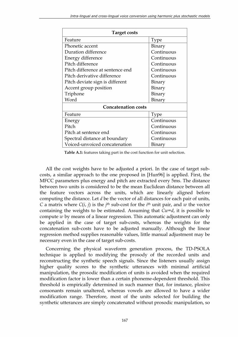
Intra-lingual and cross-lingual voice conversion using harmonic plus stochastic models
167
Target costs Feature Type Phonetic accent Binary Duration difference Continuous Energy difference Continuous Pitch difference Continuous Pitch difference at sentence end Continuous Pitch derivative difference Continuous Pitch deviate sign is different Binary Accent group position Binary Triphone Binary Word Binary
Concatenation costs Feature Type Energy Continuous Pitch Continuous Pitch at sentence end Continuous Spectral distance at boundary Continuous Voiced-unvoiced concatenation Binary Table A.1: features taking part in the cost function for unit selection.
All the cost weights have to be adjusted a priori. In the case of target sub-costs, a similar approach to the one proposed in [Hun96] is applied. First, the MFCC parameters plus energy and pitch are extracted every 5ms. The distance between two units is considered to be the mean Euclidean distance between all the feature vectors across the units, which are linearly aligned before computing the distance. Let d be the vector of all distances for each pair of units, C a matrix where C(i, j) is the jth sub-cost for the ith unit pair, and w the vector containing the weights to be estimated. Assuming that Cw=d, it is possible to compute w by means of a linear regression. This automatic adjustment can only be applied in the case of target sub-costs, whereas the weights for the concatenation sub-costs have to be adjusted manually. Although the linear regression method supplies reasonable values, little manual adjustment may be necessary even in the case of target sub-costs.
Concerning the physical waveform generation process, the TD-PSOLA technique is applied to modifying the prosody of the recorded units and reconstructing the synthetic speech signals. Since the listeners usually assign higher quality scores to the synthetic utterances with minimal artificial manipulation, the prosodic modification of units is avoided when the required modification factor is lower than a certain phoneme-dependent threshold. This threshold is empirically determined in such manner that, for instance, plosive consonants remain unaltered, whereas vowels are allowed to have a wider modification range. Therefore, most of the units selected for building the synthetic utterances are simply concatenated without prosodic manipulation, so
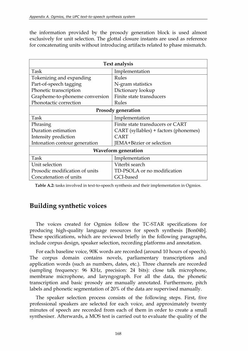
Appendix A. Ogmios, the UPC text-to-speech synthesis system
168
the information provided by the prosody generation block is used almost exclusively for unit selection. The glottal closure instants are used as reference for concatenating units without introducing artifacts related to phase mismatch.
Text analysis Task Implementation Tokenizing and expanding Rules Part-of-speech tagging N-gram statistics Phonetic transcription Dictionary lookup Grapheme-to-phoneme conversion Finite state transducers Phonotactic correction Rules
Prosody generation Task Implementation Phrasing Finite state transducers or CART Duration estimation CART (syllables) + factors (phonemes) Intensity prediction CART Intonation contour generation JEMA+Bèzier or selection
Waveform generation Task Implementation Unit selection Viterbi search Prosodic modification of units TD-PSOLA or no modification Concatenation of units GCI-based
Table A.2: tasks involved in text-to-speech synthesis and their implementation in Ogmios.
Building synthetic voices
The voices created for Ogmios follow the TC-STAR specifications for producing high-quality language resources for speech synthesis [Bon04b]. These specifications, which are reviewed briefly in the following paragraphs, include corpus design, speaker selection, recording platforms and annotation.
For each baseline voice, 90K words are recorded (around 10 hours of speech). The corpus domain contains novels, parliamentary transcriptions and application words (such as numbers, dates, etc.). Three channels are recorded (sampling frequency: 96 KHz, precision: 24 bits): close talk microphone, membrane microphone, and laryngograph. For all the data, the phonetic transcription and basic prosody are manually annotated. Furthermore, pitch labels and phonetic segmentation of 20% of the data are supervised manually.
The speaker selection process consists of the following steps. First, five professional speakers are selected for each voice, and approximately twenty minutes of speech are recorded from each of them in order to create a small synthesiser. Afterwards, a MOS test is carried out to evaluate the quality of the
Intra-lingual and cross-lingual voice conversion using harmonic plus stochastic models
169
five synthesizers. The final choice depends on several factors, such as the pleasantness of the voice, the articulation and also the result of the MOS. Only the selected speaker records the whole database.
For the baseline voices, a preliminary phonetic segmentation is computed using the UPC speech-recognition toolkit (in the forced-alignment mode) [Ade04, Ade05]. Speaker dependent models where estimated for context-dependent semi-phones. The likelihood provided by the HMM-forced alignment is used to select 20% of the sentences which have to be checked manually. The segmentation is also used by the prosody and phonetic labelling toolkit to ease the navigation through the files. After the phonetic transcription has been supervised, the files are automatically segmented again and a pruning strategy is followed to detect problematic units [Ade06]. This reduces the size of the database in 10%, but 90% of undesired units are successfully removed. The prosodic models used during synthesis are trained from the resulting database.
Pitch labels are obtained following the method described in [Per05]. The pitch epochs used for synthesis are the glottal closure instants, which are extracted from the laryngograph signal by locating the minima of the laryngograph signal derivative. Since the laryngograph signal is often noisy, pitch marks are post-processed in order to obtain a cleaner estimation. A further correction is also required to compensate the delay between the laryngograph signal and the speech signal: a low-pass filtered version of the speech signal comprising only the first harmonic is used to locate the preceding zero-crossing point, and the final pitch mark is placed on the position of the waveform minimum before the crossing-by-zero.
Performance evaluation
Ogmios participated in the 2nd TC-STAR evaluation campaign [Mos06], which intended to rate the performance of the whole TTS system in several aspects that are relevant for the assessment of the quality of speech synthesis. During the evaluation process, which was carried out via web, each subject was asked to rate, using a 5-point scale (where 1 is the worst score and 5 is the best score), different characteristics of the system. Table A.3 shows the evaluation results for several voices, including natural speech as a reference.
The scores obtained for Spanish are quite close to those of natural speech. This indicates that the performance of Ogmios in Spanish is very good. The scores obtained for English are lower because the system is optimized for Spanish and Catalan, whereas no language-specific work had been done for English before the evaluation. Taking that into account, these scores are also reasonable and prove that Ogmios can be used for building new voices in different languages in a short time.

Appendix A. Ogmios, the UPC text-to-speech synthesis system
170
Voice LE Pr C A SR N EL Pl A OQ
Spanish male 4.28 4.00 4.44 4.11 4.17 3.36 3.47 3.67 3.25 4.00 Spanish female 4.36 4.14 4.56 3.64 4.08 3.25 3.17 3.56 2.97 3.89 English female 2.92 3.02 3.49 3.25 3.83 2.26 2.13 2.82 2.28 2.84 Natural speech 4.89 4.89 4.94 4.67 4.97 4.58 4.36 4.28 4.33 4.61
Table A.3: results of the 2nd TC-STAR evaluation campaign: listening effort (LE), pronunciation (Pr), comprehension (C), articulation (A), speaking rate (SR), naturalness (N), ease of listening
(EL), pleasantness (Pl), audio flow (A) and overall quality (OQ).
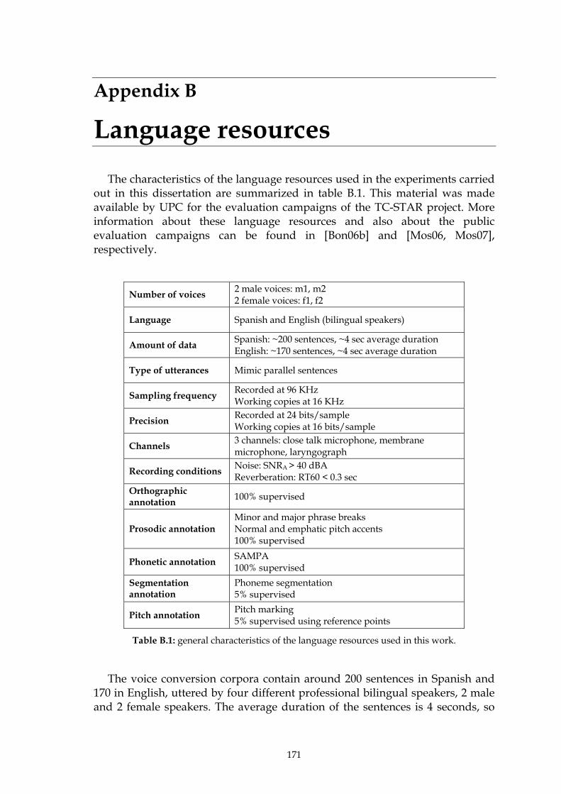
171
Appendix B
Language resources
The characteristics of the language resources used in the experiments carried out in this dissertation are summarized in table B.1. This material was made available by UPC for the evaluation campaigns of the TC-STAR project. More information about these language resources and also about the public evaluation campaigns can be found in [Bon06b] and [Mos06, Mos07], respectively.
Number of voices 2 male voices: m1, m2 2 female voices: f1, f2
Language Spanish and English (bilingual speakers)
Amount of data Spanish: ~200 sentences, ~4 sec average duration English: ~170 sentences, ~4 sec average duration
Type of utterances Mimic parallel sentences
Sampling frequency Recorded at 96 KHz Working copies at 16 KHz
Precision Recorded at 24 bits/sample Working copies at 16 bits/sample
Channels 3 channels: close talk microphone, membrane microphone, laryngograph
Recording conditions Noise: SNRA > 40 dBA Reverberation: RT60 < 0.3 sec
Orthographic annotation 100% supervised
Prosodic annotation Minor and major phrase breaks Normal and emphatic pitch accents 100% supervised
Phonetic annotation SAMPA 100% supervised
Segmentation annotation
Phoneme segmentation 5% supervised
Pitch annotation Pitch marking 5% supervised using reference points
Table B.1: general characteristics of the language resources used in this work.
The voice conversion corpora contain around 200 sentences in Spanish and 170 in English, uttered by four different professional bilingual speakers, 2 male and 2 female speakers. The average duration of the sentences is 4 seconds, so
Appendix B: Language resources
172
between 10 and 15 minutes of audio are available for each speaker and language. The fact that the speakers are bilingual allows researching not only into intra-lingual voice conversion but also into cross-lingual voice conversion. From now on, the recorded voices will be denoted m1, m2, f1 and f2, as indicated in table B.1.
The sentences uttered by the speakers are exactly the same, so that parallel training corpora can be used for training voice conversion functions. In addition, the sentences were recorded as mimic sentences. This means that the recordings were made in such manner that there were no significant prosodic differences between speakers, since they all were asked to imitate the same pre-recorded pattern with neutral speaking style for each of the sentences [Kai01]. This allows the listeners that participate in the perceptual tests concentrating on the spectral characteristics of voice, so that the spectral envelope conversion methods can be evaluated in a more precise way.
The recordings were made in a soundproof chamber whose signal to noise ratio was higher than 40dBA and whose reverberation time at 60dB was lower than 0.3 seconds. Initially the audio files were recorded at 96 KHz sampling frequency and 24 bits per sample, but the working copies used for this research work were converted to 16 KHz - 16 bits format. Although 3 different audio channels were available (close talk microphone, membrane microphone and laryngograph), only the one coming from the membrane microphone was used in this work.
Each audio file was stored together with the following information: the prompt text used to record the utterance, the orthographic annotation, the phonetic transcription, the segmentation into phonemes, and the pitch marks centered at the glottal closure instants. The phonetic transcription was carried out manually. During the automatic segmentation, the starting and ending time instants of the transcribed phonemes were determined. The pitch marks were also automatically estimated: first, the electroglotographic signal was differentiated to find out the negative peaks that correspond to the glottal closure instant; second, the speech signal was filtered by a low-pass filter; finally, in order to synchronize the pitch marks with the speech signal, the estimated glottal closure instants were delayed to match the minimum-energy instants located just before the waveform peaks. In the present work, the usage of all this extra information has been avoided as far as possible, in order to make the system more versatile and less information-demanding. However, the data coming from the segmentation have been used for aligning the frames of the parallel sentences in a reliable way (see chapter 4).
173
Bibliography [Abe88] M. Abe, S. Nakamura, K. Shikano, H. Kuwabara, “Voice conversion through vector
quantization”, Proc. IEEE Int. Conf. on Acoustics, Speech and Signal Processing, pp.655-658, 1988.
[Abe90] M. Abe, K. Shikano, H. Kuwabara, “Cross-language voice conversion”, Proc. IEEE Int. Conf. on Acoustics, Speech and Signal Processing, pp.345-348, 1990.
[Abr91] A.J. Abrantes, J.S. Marques, I.M. Trancoso, “Hybrid sinusoidal modeling of speech without voicing decision”, Eurospeech, 1991.
[Ade04] J. Adell, A. Bonafonte, “Towards phone segmentation for concatenative speech synthesis”, 5th ISCA Speech Synthesis Workshop, pp.139-144, 2004.
[Ade05] J. Adell, A. Bonafonte, J.A. Gómez, M.J. Castro, “Comparative study of automatic phone segmentation methods for TTS”, Proc. of IEEE Int. Conf. on Acoustics Speech and Signal Processing, 2005.
[Ade06] J. Adell, P.D. Agüero, A. Bonafonte, “Database pruning for unsupervised building of text-to-speech voice”, Proceedings of ICASSP, 2006.
[Agü04a] P.D. Agüero, A. Bonafonte, “Intonation modeling for TTS using a joint extraction and prediction approach”, Proceedings of the International Workshop on Speech Synthesis, 2004.
[Agü04b] P.D. Agüero, K. Wimmer, A. Bonafonte, “Joint extraction and prediction of Fujisaki's intonation model parameters”, Proceedings of International Conference on Spoken Language Processing, 2004.
[Agü05] P.D. Agüero, A. Bonafonte, “Consistent estimation of Fujisaki's intonation model parameters”, International Conference on Speech and Computer, SPECOM, 2005.
[Agü06] P.D. Agüero, J. Adell, A. Bonafonte, “Prosody generation for speech-to-speech translation”, Proc. IEEE Int. Conf. on Acoustics, Speech and Signal Processing, pp.557-560, 2006.
[Ahm98] S. Ahmadi, A.S. Spanias, “A new phase model for sinusoidal transform coding of speech”, IEEE Transactions on Speech and Audio Processing, vol.6, nº5, pp.495-, 1998.
[Ahn97] R. Ahn, W.H. Holmes, “An improved harmonic-plus-noise decomposition method and its application in pitch determination”, IEEE Workshop on Speech Coding for Telecommunications, pp.41-42, 1997.
[Alk91] P. Alku, E. Vilkman, U.K. Laine, “Analysis of glottal waveform in different phonation types using the new IAIF method”, Proc. Int. Congr. Phonetic Sciences, 1991.
[Alm82] L.B. Almeida, J.M. Tribolet, “Harmonic coding: a low bit-rate, good-quality speech coding technique”, Proc. IEEE Int. Conf. on Acoustics, Speech and Signal Processing, vol.7, pp.1664-1667, 1982.
[Alm83] L.B. Almeida, J.M. Tribolet, “Nonstationary spectral modeling of voiced speech”, IEEE Transactions on Acoustics, Speech and Signal Processing, vol.31, nº3, pp.664-678, 1983.
[Alm84] L.B. Almeida, F.M. Silva, “Variable frequency synthesis: an improved harmonic coding scheme”, Proc. IEEE Int. Conf. on Acoustics, Speech and Signal Processing, vol.9, pp.437-440, 1984.
Bibliography
174
[Ars98] L.M. Arslan, D. Talkin, “Speaker transformation using sentence HMM based alignments and detailed prosody modification”, Proc. IEEE Int. Conf. on Acoustics, Speech and Signal Processing, vol.1 pp.289-292, 1998.
[Ars99] L.M. Arslan, “Speaker transformation algorithm using segmental codebooks (STASC)”, Speech Communication, no.28, 1999.
[Bai01] G. Bailly, “A parametric harmonic + noise model”, chapter in “Improvements in Speech Synthesis”, John Wiley & Sons Ltd., pp.22-38, 2002.
[Bau96] G. Baudoin, Y. Stylianou, “On the transformation of the speech spectrum for voice conversion”, Proc. of the Int. Conf. on Spoken Language Processing, vol.3 pp.1405-1408, 1996.
[Boe93] P. Boersma, “Accurate short-term analysis of the fundamental frequency and the harmonics-to-noise ratio of a sampled sound”, Proceedings of the Institute of Phonetic Sciences, University of Amsterdam, vol.17, 1993.
[Bon04a] A. Bonafonte, P.D. Agüero, “Phrase break prediction using a finite state transducer”, in Proc. of the 11th International Workshop on Advances in Speech Technology, Maribor, Slovenia, July 2004.
[Bon04b] A. Bonafonte, H. Höge, H.S. Tropf, A. Moreno, H. van der Heuvel, D. Sündermann, U. Ziegenhain, J. Pérez, I. Kiss, “Deliverable D8: TTS - baselines and specifications”, technical report for TC-STAR project, http://www.tcstar.org, 2004.
[Bon06a] A. Bonafonte, P.D. Agüero, J. Adell, J. Pérez, A. Moreno, “OGMIOS: The UPC text-to-speech synthesis system for spoken translation”, TC-Star Workshop on Speech to Speech Translation, 2006.
[Bon06b] A. Bonafonte, H. Höge, I. Kiss, A. Moreno, U. Ziegenhain, H. van den Heuvel, H.U. Hain, X.S. Wang, M.N. Garcia, “TC-STAR: specifications of language resources and evaluation for speech synthesis”, Int. Conf. on Language Resources and Evaluation, 2006.
[Bon07] A. Bonafonte, J. Adell, P.D. Agüero, D. Erro, I. Esquerra, A. Moreno, J. Pérez, T. Polyakova, “The UPC TTS system description for the 2007 Blizzard Challenge”, 6th ISCA Workshop on Speech Synthesis, 2007.
[Cey02] T. Ceyssens, W. Verhelst, P. Wambacq, “On the construction of a pitch conversion system”, Proc. of the European Signal Processing Conference, vol.1 pp.423-426, 2002.
[Cha98] D.T. Chappell, J.H.L. Hansen, “Speaker specific pitch contour modeling and modification”, International Conference on Acoustics, Speech and Signal Processing, 1998.
[Cha02] D. Chazan, R. Hoory, Z. Kons, D. Silberstein, A. Sorin, “Reducing the footprint of the IBM trainable speech synthesis system”, Proc.7th Int. Conf. Spoken Language Processing, 2002.
[Cha06] D. Chazan, R. Hoory, A. Sagi, S. Shechtman, A. Sorin, Z.W. Shuang, R. Bakis, “High quality sinusoidal modeling of wideband speech for the purposes of speech synthesis and modification”, Proc. ICASSP, 2006.
[Che03] Y. Chen, M. Chu, E. Chang, J. Liu, R. Liu, “Voice conversion with smoothed GMM and MAP adaptation”, European Conference on Speech Communications and Technology, pp.2413-2416, 2003.
[Dep97] Ph. Depalle, T. Hélie, “Extraction of spectral peak parameters using a STFT modeling and no-sidelobe windows”, Proceedings of the IEEE Workshop on Applications of Signal Processing to Audio and Acoustics, 1997.
[Dur60] J. Durbin, “The fitting of time series models”, Rev. Inst. Int. Stat., vol.28, pp.233-243, 1960.
Intra-lingual and cross-lingual voice conversion using harmonic plus stochastic models
175
[Dux04] H. Duxans, A. Bonafonte, A. Kain, J. van Santen, “Including dynamic and phonetic information in voice conversion systems”, Proc. of the Int. Conf. on Spoken Language Processing, pp.1193-1196, 2004.
[Dux06a] H. Duxans, A. Bonafonte , “Residual conversion versus prediction on voice morphing systems”, Proc. IEEE Int. Conf. on Acoustics, Speech and Signal Processing, vol.1 pp.85-88, 2006.
[Dux06b] H. Duxans, D. Erro, J. Pérez, F. Diego, A. Bonafonte, A. Moreno, “Voice conversion of non-aligned data using unit selection”, TC-STAR Workshop on Speech to Speech Translation, 2006.
[Elj91] A. El-Jaroudi, J. Makhoul, “Discrete all-pole modeling”, IEEE Transactions on Signal Processing, vol.39, no.2, pp.411-, 1991.
[Enn04] T. En-Najjary, O. Rosec, T. Chonavel, “A voice conversion method based on joint pitch and spectral envelope transformation”, Proc. of the Int. Conf. on Spoken Language Processing, pp.1225-1228, 2004.
[Enn05] T. En-Najjary, “Conversion de voix pour la synthèse de la parole”, PhD thesis, Université de Rennes I, 2005.
[Err05] D. Erro, A. Moreno, “A pitch-asynchronous simple method for speech synthesis by diphone concatenation using the deterministic plus stochastic model”, Proc. 10th Int. Conf. on Speech and Computer, pp.321-324, 2005.
[Err06a] D. Erro, A. Moreno, “Efficient Speech Synthesis System using the Deterministic plus Stochastic Model”, Speech Prosody, 2006.
[Err06b] D. Erro, A. Moreno, “Sistema de síntesis armónico/estocástico en modo pitch-asíncrono aplicado a conversión de voz”, IV Jornadas en Tecnologías del Habla, 2006.
[Err07a] D. Erro, A. Moreno, “Weighted frequency warping for voice conversion”, Interspeech, 2007.
[Err07b] D. Erro, A. Moreno, “Frame alignment method for cross-lingual voice conversion”, Interspeech, 2007.
[Err07c] D. Erro, A. Moreno, A. Bonafonte, “Flexible harmonic/stochastic speech synthesis”, 6th ISCA Workshop on Speech Synthesis, 2007.
[Err08] D. Erro, T. Polyakova, A. Moreno, “On combining statistical methods and frequency warping for high-quality voice conversion”, in Proc. IEEE Int. Conf. on Acoustics, Speech, and Signal Processing, 2008.
[Fur86] S. Furui, “Research on individuality features in speech waves and automatic speaker recognition techniques”, Speech Communication, vol.5, no.2, pp.183-197, 1986.
[Geo87] E.B. George, M.J.T. Smith, “A new speech coding model based on a least-squares sinusoidal representation”, in Proc. IEEE Int. Conf. on Acoustics, Speech, and Signal Processing, pp. 1641-1644, 1987.
[Geo92] E.B. George, M.J.T. Smith, “An analysis-by-synthesis approach to sinusoidal modeling applied to the analysis and synthesis of musical tones”, Journal of the Audio Engineering Society, vol.40, pp.497-516, 1992.
[Geo97] E.B. George, M.J.T. Smith , “Speech analysis/synthesis and modification using an analysis-by-synthesis/overlap-add sinusoidal model”, IEEE Transactions on Speech and Audio Processing, vol.5, nº5, pp.389-, 1997.
[Gil03] B. Gillett, S. King, “Transforming f0 contours”, European Conference on Speech Communications and Technology, pp.101-104, 2003.
[Gri88] D.W. Griffin, J.S. Lim, “Multiband excitation vocoder”, IEEE Transactions on Acoustics, Speech and Signal Processing, 1988.
Bibliography
176
[Gut98] J.M. Gutiérrez-Arriola, Y.S. Hsiao, J.M. Montero, J.M. Pardo, D.G. Childers, “Voice conversion based on parameter transformation”, Proc. of the ICSLP, vol.3, pp.987-990, 1998.
[Gut01] J.M. Gutiérrez-Arriola, J.M. Montero, J.A. Vallejo, R. de Córdoba, R. San Segundo, J.M. Pardo, “A new multi-speaker formant synthesizer that applies voice conversion techniques”, 7th European Conference on Speech Communication and Technology, Eurospeech, vol.1, pp.357-360, 2001.
[Han07] Z. Hanzlicek, J. Matousek, “F0 transformation within the voice conversion framework”, Interspeech, 2007.
[Hed81] P. Hedelin, “A tone-oriented voice-excited vocoder”, International Conference on Acoustics, Speech and Signal Processing, 1981.
[Hel07] E.E. Helander, J. Nurminen, “A novel method for prosody prediction in voice conversion”, International Conference on Acoustics, Speech and Signal Processing, 2007.
[Her91] D.J. Hermes, “Synthesis of breathy vowels: some research methods”, Speech Communication, vol.10, no.5-6, pp.497-, 1991.
[Hsi07] C.C. Hsia, C.H. Wu, J.Q. Wu, “Conversion function clustering and selection using linguistic and spectral information for emotional voice conversion”, IEEE Transactions on Computers, vol.56, nº9, pp.1245-, 2007.
[Hua01] X. Huang, A. Acero, H.W. Hon, “Spoken language processing: a guide to theory, algorithm and system development”, Prentice Hall, 2001.
[Hun96] A. Hunt, A. Black, “Unit selection in a concatenative speech synthesis system using a large speech database”, in Proc. of ICASSP, 1996.
[Ina03] Z. Inanoglu, “Transforming pitch in a voice conversion framework”, M.S. Thesis, University of Cambridge, 2003.
[Ito82] K. Itoh, S. Saito, "Effects of acoustical feature parameters of speech on perceptual identification of speaker", IECE Trans., vol.J65-A, pp.101-108, 1982.
[Iwa94] N. Iwahashi, Y. Sagisaka, “Speech spectrum transformation by speaker interpolation”, Proc. IEEE Int. Conf. on Acoustics, Speech and Signal Processing, vol.1 pp.461-464, 1994.
[Iwa95] N. Iwahashi, Y. Sagisaka, “Speech spectrum conversion based on speaker interpolation and multi-functional representation with weighting by radial basis function networks”, Speech Communication, vol.16 no.2 pp.139-151, 1995.
[Kai01] A. Kain, “High resolution voice transformation”, PhD thesis, OGI school of science and engineering, 2001.
[Kaw97] H. Kawahara , “Speech representation and transformation using adaptive interpolation of weighted spectrum: vocoder revisited”, Proc. IEEE Int. Conf. on Acoustics, Speech and Signal Processing, vol.2 p.1303, 1997.
[Kaw03] H. Kawanami, Y. Iwami, T. Toda, H. Saruwatari, K. Shikano, “GMM-based voice conversion applied to emotional speech synthesis”, 8th European Conference on Speech Communication and Technology, Interspeech-Eurospeech, 2003.
[Kum03] A. Kumar, A. Verma, “Using phone and diphone based acoustic models for voice conversion: a step towards creating voice fonts”, Proc. IEEE Int. Conf. on Acoustics, Speech and Signal Processing, vol.1 pp.720-723, 2003.
[Kuw95] H. Kuwabara, Y. Sagisaka, “Acoustic characteristics of speaker individuality: control and conversion”, Speech Communication, vol.16, no.2, pp.165-173, 1995.
Intra-lingual and cross-lingual voice conversion using harmonic plus stochastic models
177
[Lar93] J. Laroche, Y. Stylianou, E. Moulines , “HNM: a simple, efficient harmonic+noise model for speech”, Proc. IEEE ICASSP, 1993.
[Lat06] J. Latorre, K. Iwano, S. Furui, “New approach to the polyglot speech generation by means of an HMM-based speaker adaptable synthesizer”, Speech Communication, vol.48 no.10 pp.1227-1242, 2006.
[Lee06] C.H. Lee, C.H. Wu , “MAP-based adaptation for speech conversion using adaptation data selection and non-parallel training”, Proc. of the Int. Conf. on Spoken Language Processing, 2006.
[Lee07] K.S. Lee, “Statistical approach for voice personality transformation”, IEEE Transactions on Audio, Speech and Language Processing, vol.15 no.2 pp.641-651, 2007.
[Lev47] N. Levinson, “The wiener RMS error criterion in filter design and prediction”, J. Math. Phys., vol. 25, pp.261-278, 1947.
[Mac96] M.W. Macon, M.A. Clements, “Speech concatenation and synthesis using an overlap-add sinusoidal model”, Proc. ICASSP, pp.361-364, 1996.
[Mac97] M.W. Macon, M.A. Clements , “Sinusoidal modeling and modification of unvoiced speech”, IEEE Transactions on Speech and Audio Processing, vol.5, nº6, pp.557-560, 1997.
[Mak75] J. Makhoul, “Linear prediction: a tutorial review”, Proc. of the IEEE, vol.63, no.5, pp.561-580, 1975.
[Mar90] J.S. Marques, L.B. Almeida, J.M. Tribolet, “Harmonic coding at 4.8 KB/s”, Proc. IEEE Int. Conf. on Acoustics, Speech and Signal Processing, 1990.
[Mas01] M. Mashimo, T. Toda, K. Shikano, N. Campbell, “Evaluation of Cross-language Voice Conversion Based on GMM and STRAIGHT”, European Conference on Speech Communications and Technology, pp.361-364, 2001.
[Mas96] T. Masuko, K. Tokuda, T. Kobayashi, S. Imai, “Speech synthesis using HMMs with dynamic features”, Proc. IEEE Int. Conf. on Acoustics, Speech and Signal Processing, pp.389-392, 1996.
[Mas97] T. Masuko, K. Tokuda, T. Kobayashi, S. Imai, “Voice characteristics conversion for HMM-based speech synthesis system”, Proc. IEEE Int. Conf. on Acoustics, Speech and Signal Processing, pp.1611-1614, 1997.
[Mat73] H. Matsumoto, S. Hiki, T. Sone, T. Nimura, "Multidimensional representation of personal quality of vowels and its acoustical correlates", IEEE Transactions on Audio and Electroacoustics, vol.21, no.5, pp.428-436, 1973.
[Mca84] R.J. McAulay, T.F. Quatieri, “Magnitude-only reconstruction using a sinusoidal speech model”, Proc. IEEE Int. Conf. on Acoustics, Speech and Signal Processing, 1984.
[Mca86a] R.J. McAulay, T.F. Quatieri, “Speech analysis/synthesis based on a sinusoidal representation”, IEEE Transactions on Acoustics, Speech and Signal Processing, vol.34 no.4 pp.744–754, 1986.
[Mca86b] R.J. McAulay, T.F. Quatieri, “Speech transformation based on a sinusoidal representation”, IEEE Transactions on Acoustics, Speech and Signal Processing, vol.34 no.6 pp.1449-, 1986.
[Mca95] R.J. McAulay, T.F. Quatieri, “Sinusoidal coding”, Speech Coding and Synthesis, Chapter 4, W.B. Kleijn, and K.K. Paliwal Eds., Elsevier, 1995.
[Mes07] L. Mesbahi, V. Barreaud, O. Boeffard, “GMM-based speech transformation systems under data reduction”, 6th ISCA Workshop on Speech Synthesis, 2007.
Bibliography
178
[Miz94] H. Mizuno, M. Abe, “Voice conversion based on piecewise linear conversion rules of formant frequency and spectrum tilt”, Proc. IEEE Int. Conf. on Acoustics, Speech and Signal Processing, vol.1 pp.469-472, 1994.
[Mor03] H. Mori, H. Kasuya, “Speaker conversion in ARX-based source-formant type speech synthesis”, European Conference on Speech Communications and Technology, pp.2421-2424, 2003.
[Mos06] D. Mostefa, M.N. Garcia, O. Hamon, N. Moreau, Evaluation Report, Deliverable D16 of the EU funded project TC-STAR, http://www.tc-star.org, 2006.
[Mos07] D. Mostefa, O. Hamon, N. Moreau, K. Choukri, Evaluation Report, Deliverable D30 of the EU funded project TC-STAR, http://www.tc-star.org, 2007.
[Mou06] A. Mouchtaris, J. Van der Spiegel, P. Mueller , “Nonparallel training for voice conversion based on a parameter adaptation approach”, IEEE Transactions on Audio, Speech and Language Processing, vol.14 no.3 pp.952-963, 2006.
[Mou90] E. Moulines, F. Charpentier, “Pitch-synchronous waveform processing techniques for text-to-speech synthesis using diphones”, Speech Communication, vol.9 no.5-6 pp.453-467, 1990.
[Mou95] E. Moulines, W. Verhelst, “Time-domain and frequency-domain techniques for prosodic modification of speech”, Speech coding and synthesis, Elsevier Science B.V., pp.519-555, 1995.
[Nan07] Y. Nankaku, K. Nakamura, T. Toda, K. Tokuda, “Spectral conversion based on statistical models including time-sequence matching”, 6th ISCA Workshop on Speech Synthesis, 2007.
[Nar95] M. Narendranath, H.A. Murthy, S. Rajendran, B. Yegnanarayana, “Transformation of formants for voice conversion using artificial neural networks”, Speech communication, vol.16 no.2 pp.207-216, 1995.
[Obr01] D. O'Brien, A.I.C. Monaghan, “Concatenative synthesis based on a harmonic model”, IEEE Transactions on Speech and Audio Processing, vol.9, nº1, pp.11-, 2001.
[Oht07a] Y. Ohtani, T. Toda, H. Saruwatari, K. Shikano, “Speaker adaptive training for one-to-many eigenvoice conversion based on gaussian mixture model”, Interspeech, 2007.
[Oht07b] K. Ohta, Y. Ohtani, T. Toda, H. Saruwatari, K. Shikano, “Regression approaches to voice quality control based on one-to-many eigenvoice conversion”, 6th ISCA Workshop on Speech Synthesis, 2007.
[Pau81] D.B. Paul, “The spectral envelope estimation vocoder”, IEEE Transactions on Acoustics, Speech and Signal Processing, vol.29, no.4, pp.786-794, 1981.
[Per05] J. Pérez, A. Bonafonte, “Automatic voice source parameterization of natural speech”, Interspeech, 2005.
[Per06] J. Pérez, A. Bonafonte, H.U. Hain, E. Keller, S. Breuer, J. Tian, “ECESS inter-module interface specification for speech synthesis”, Proceedings of LREC Conference, 2006.
[Per07] W.S. Percybrooks, E. Moore II, “New algorithm for LPC residual estimation from LSF vectors for a voice conversion system”, Interspeech, 2007.
[Pol06] T. Polyakova, A. Bonafonte, “Learning from errors in Grapheme-to-Phoneme Conversion”, Proc. of International Conference on Spoken Language Processing, ISCLP, Pittsburgh, USA, 2006.
[Pol07] T. Polyakova, A. Bonafonte, “Fusion of dictionaries in voice creation and synthesis task”, Proc. of the 12th International conference on Speech and Computer, SPECOM, 2007.
Intra-lingual and cross-lingual voice conversion using harmonic plus stochastic models
179
[Pri06] A. Pribilova, J. Pribil, “Non-linear frequency scale mapping for voice conversion in text-to-speech system with cepstral description”, Speech Communication, vol.48, pp.1691-1703, 2006.
[Qua92] T.F. Quatieri, R.J. McAulay , “Shape invariant time-scale and pitch modification of speech”, IEEE Transactions on Signal Processing, vol.40 no.3 pp.497-510, 1992.
[Ren04] D. Rentzos, S. Vaseghi, Q. Yan, C.H. Ho, “Voice conversion through transformation of spectral and intonation features”, Proc. IEEE Int. Conf. on Acoustics, Speech and Signal Processing, vol.1 pp.21-24, 2004.
[Ric96] G. Richard, C. d'Alessandro, “Analysis/synthesis and modification of the speech aperiodic component”, Speech Communication, 1996.
[Rod92] X. Rodet, P. Depalle, “Spectral envelopes and inverse FFT synthesis”, Convention of the audio engineering society, AES 1992.
[Rod97] X. Rodet, “Musical sound signal analysis/synthesis: sinusoidal+residual and elementary waveform models”, Proceedings of the IEEE Time-Frequency and Time-Scale Workshop, 1997.
[Rod02] E. Rodríguez-Banga, C. García-Mateo, X. Fernández-Salgado, “Concatenative text-to-speech synthesis based on sinusoidal modelling”, chapter in "Improvements in Speech Synthesis", John Wiley & Sons Ltd., pp.52-63, 2002.
[Roj05] M. Rojc, P.D. Agüero, A. Bonafonte, Z. Kacic, “Training the Tilt intonation model using the JEMA methodology”, Eurospeech, 2005.
[Sal06] Ö. Salor, M. Demirekler, “Dynamic programming approach to voice transformation”, Speech Communication, vol.48 no.10 pp.1262-1272, 2006.
[Sat74] H. Sato, “Acoustic cues of female voice quality”, Electronics and Communication in Japan, 57-A, pp.29-38, 1974.
[Ser89] X. Serra, “A system for sound analysis/transformation/synthesis based on a deterministic plus stochastic decomposition”, PhD. Dissertation, Stanford University, 1989.
[Ser97] X. Serra, “Musical sound modeling with sinusoids plus noise”, Musical Signal Processing, p. Swets & Zeitlinger Publishers, 1997.
[Shi91] K. Shikano, S. Nakamura, M. Abe, “Speaker adaptation and voice conversion by codebook mapping”, IEEE International Symposium on Circuits and Systems, vol.1 pp.594-597,1991.
[Shu06] Z.W. Shuang, R. Bakis, S. Shechtman, D. Chazan, Y. Qin, “Frequency warping based on mapping formant parameters”, Proc. of the Int. Conf. on Spoken Language Processing, 2006.
[Smi87] J. Smith, X. Serra, “PARSHL: an analysis/synthesis program for non-harmonic sounds based on a sinusoidal representation”, Proceedings of International Computer Music Conference, 1987.
[Sty95] Y. Stylianou, J. Laroche, E. Moulines, “High-quality speech modification based on a harmonic+noise model”, Proc. Eurospeech, 1995.
[Sty96] Y. Stylianou, “Harmonic plus Noise Models for Speech, combined with Statistical Methods, for Speech and Speaker Modification”, PhD thesis, École Nationale Supérieure des Télécommunications, 1996.
[Sty98] Y. Stylianou, O. Cappé, E. Moulines, “Continuous probabilistic transform for voice conversion”, Proc. IEEE Int. Conf. on Acoustics, Speech and Signal Processing, vol.6 no.2 pp.131-142, 1998.
Bibliography
180
[Sty00] Y. Stylianou, “On the implementation of the HNM for concatenative speech synthesis”, Proc. IEEE ICASSP, 2000.
[Sty01a] Y. Stylianou, “Applying the HNM in concatenative speech synthesis”, IEEE Transactions on speech and audio processing, vol.9, nº1, pp.21-, 2001.
[Sty01b] Y. Stylianou, “Removing linear phase mismatches in concatenative speech synthesis”, IEEE Transactions on Speech and Audio Processing, vol.9, no.3, pp.232-, 2001.
[Sty07] Y. Stylianou, “Voice transformation”, Tutorial at Interspeech, 2007.
[Sün03a] D. Sündermann, H.Ney, “VTLN-based voice conversion”, Proc. of the IEEE Symposium on Signal Processing and Information Technology, 2003.
[Sün03b] D. Sündermann, H. Ney, H. Höge, “VTLN-based cross-language voice conversion”, Proc. of the IEEE Automatic Speech Recognition and Understanding Workshop, pp.676-681, 2003.
[Sün04] D. Sündermann, A. Bonafonte, H. Ney, H. Höge, “A first step towards text-independent voice conversion”, Proc. of the Int. Conf. on Spoken Language Processing, pp.1173-1176, 2004.
[Sün05] D. Sündermann, H. Höge, A. Bonafonte, H. Duxans, “Residual prediction”, Proc. of the IEEE Symposium on Signal Processing and Information Technology, pp.512-516, 2005.
[Sün06a] D. Sündermann, H. Höge, A. Bonafonte, H. Ney, A. Black, S. Narayanan, “Text-independent voice conversion based on unit selection”, Proc. IEEE Int. Conf. on Acoustics, Speech and Signal Processing, vol.1 pp.81-84, 2006.
[Sün06b] D. Sündermann, H. Höge, A. Bonafonte, H. Ney, and J. Hirschberg, “Text-independent cross-language voice conversion”, Proc. of the Int. Conf. on Spoken Language Processing, 2006.
[Syr98] A. Syrdal, Y. Stylianou, L. Garrison, A. Conkie, J. Schroeter, “TD-PSOLA versus HNM in diphone based speech synthesis”, Proc. ICASSP, 1998.
[Tam98] M. Tamura, T. Masuko, K. Tokuda, T. Kobayashi, “Speaker adaptation for HMM-based speech synthesis system using MLLR”, Proc. ESCA/COCOSDA Workshop on Speech Synthesis, pp.273-276, 1998.
[Tam01] M. Tamura, T. Masuko, K. Tokuda, T. Kobayashi, “Text-to-speech synthesis with arbitrary speaker's voice from average voice”, European Conference on Speech Communications and Technology, pp.345-348, 2001.
[Tod01] T. Toda, H. Saruwatari, K. Shikano, “Voice conversion algorithm based on gaussian mixture model with dynamic frequency warping of STRAIGHT spectrum”, Proc. IEEE Int. Conf. on Acoustics, Speech and Signal Processing, pp.841-844, 2001.
[Tod05] T. Toda, A.W. Black, K. Tokuda, “Spectral conversion based on maximum likelihood estimation considering global variance of converted parameter”, Proc. IEEE Int. Conf. on Acoustics, Speech and Signal Processing, vol.1 pp.9-12, 2005.
[Tod06] T. Toda, Y. Ohtani, K. Shikano, “Eigenvoice conversion based on gaussian mixture model”, Proc. of the Int. Conf. on Spoken Language Processing, 2006.
[Tur06] O. Turk, L.M. Arslan, “Robust processing techniques for voice conversion”, Computer Speech and Language, vol.20 no.4 pp.441-467, 2006.
[Val92] H. Valbret, E. Moulines, J.P. Tubach, “Voice transformation using PSOLA technique”, Speech Communication, vol.1 pp.145-148, 1992.
[Ver05] A. Verma, A. Kumar, “Voice fonts for individuality representation and transformation”, ACM Transactions on Speech and Language Processing, vol.2, no.1, 2005.
Intra-lingual and cross-lingual voice conversion using harmonic plus stochastic models
181
[Vin07] D. Vincent, O. Rosec, T. Chonavel, “A new method for speech synthesis and transformation based on a ARX-LF source-filter decomposition and HNM modeling”, International Conference on Acoustics, Speech and Signal Processing, 2007.
[Vio98] F. Violaro, O. Boeffard, “A hybrid model for text-to-speech synthesis”, IEEE Transactions on Speech and Audio Processing, 1998.
[Wat02] T. Watanabe, T. Murakami, M. Namba, T. Hoya, Y. Ishida, “Transformation of spectral envelope for voice conversion based on radial basis function networks”, Proc. of the Int. Conf. on Spoken Language Processing, pp.285-288, 2002.
[Wu06] C.H. Wu, C.C. Hsia, T.H. Liu, J.F. Wang, “Voice conversion using duration-embedded Bi-HMMs for expressive speech synthesis”, IEEE Transactions on Audio, Speech and Language Processing, vol.14, nº4, pp.1109-, 2006.
[Ye04a] H. Ye, S. Young, “High quality voice morphing”, Proc. IEEE Int. Conf. on Acoustics, Speech and Signal Processing, vol.1 pp.9-12, 2004.
[Ye04b] H. Ye, S. Young, “Voice conversion for unknown speakers”, Proc. of the Int. Conf. on Spoken Language Processing, pp.1161-1164, 2004.
[Ye06] H. Ye, S. Young, “Quality-enhanced voice morphing using maximum likelihood transformations”, IEEE Transactions on Audio, Speech and Language Processing, vol.14 no.4 pp.1301-1312, 2006.
[Yeg98] B. Yegnanarayana, C. d'Alessandro, V. Darsinos, “An iterative algorithm for decomposition of speech signals into periodic and aperiodic components”, IEEE Transactions on Speech and Audio Processing, 1998.
[Zen07] H. Zen, T. Nose, J. Yamagishi, S. Sako, T. Masuko, A.W. Black, K. Tokuda, “The HMM-based synthesis system (HTS) version 2.0”, 6th ISCA Workshop on Speech Synthesis, 2007.