Technical Report Documentation Page   1.  Report No. SWUTC/02/167403-1 

 2.  Government Accession No.  

 3.  Recipient's Catalog No.   5.  Report Date March 2002 

 4.  Title and Subtitle Sustainable Transportation:  Conceptualization and Performance Measures     6.  Performing Organization Code 

  7.  Author(s) Josias Zietsman and Laurence R. Rilett 

 8.  Performing Organization Report No. Report  167403 10.  Work Unit No. (TRAIS)  

 9.  Performing Organization Name and Address Texas Transportation Institute The Texas A&M University System College Station, Texas  77843-3135   

11.  Contract or Grant No.  10727 13.  Type of Report and Period Covered   

12.  Sponsoring Agency Name and Address Southwest Region University Transportation Center Texas Transportation Institute The Texas A&M University System College Station, Texas  77843-3135   

14.  Sponsoring Agency Code  

15.  Supplementary Notes Supported by general revenues from the State of Texas 16.  Abstract      Sustainable transportation attempts to address economic development, environmental stewardship, and social equity of current and future generations. While numerous qualitative studies have been performed on this topic, there has been little quantitative research and/or implementation of sustainable transportation concepts. The main reasons for this are related to a lack of understanding of sustainable transportation and a lack of quantified performance measures. To address this problem, a comprehensive definition for sustainable transportation was developed, as well as a framework on how to identify, quantify, and use performance measures for sustainable transportation in the transportation planning process. The proposed framework was applied to a test bed, comprising two freeway corridors in Houston, Texas.    New innovations such as Automatic Vehicle Identification (AVI) data and the Transportation Analysis and Simulation System (TRANSIMS) model make it possible to obtain travel-related information at highly disaggregate levels. This information can be used to quantify sustainable transportation performance measures at the individual level and levels of spatial and temporal disaggregation, which has previously not been possible. The AVI data, the TRANSIMS model, and a number of transportation environmental impact models were used to quantify the performance measures at various levels of aggregation.    The performance measures that were quantified on disaggregate levels were compared to measures that were quantified with traditional aggregate data sets. It was found that the traditional approach is much less accurate due to a loss of detail and the effect of aggregation bias. It was illustrated that the performance measures based on disaggregate data can potentially provide different results as compared to aggregate approaches, when used with multi-objective decision-making techniques in transportation planning. Finally, it was demonstrated that the disaggregate approach can be used to allocate responsibility for negative externalities, and to assess the sustainability as experienced by different user groups.     17.  Key Words Sustainable Transportation, Performance Measures, Disaggregate, Decision-Making, TRANSIMS, AVI Data 

18.  Distribution Statement No restrictions.  This document is available to the public through NTIS: National Technical Information Service 5285 Port Royal Road Springfield, Virginia  22161 

19.  Security Classif.(of this report) Unclassified 

20.  Security Classif.(of this page) Unclassified 

21.  No. of Pages 163 

22.  Price  

  Form DOT F 1700.7 (8-72)                       Reproduction of completed page authorized 

 

 

 

 

SUSTAINABLE TRANSPORTATION:  CONCEPTUALIZATION AND 

PERFORMANCE MEASURES 

 

 

By 

 

Josias Zietsman Associate Research Scientist Texas Transportation Institute 

 and  

Laurence R. Rilett Associate Professor 

Texas A&M University          

Research Report SWUTC/02/167403-1  

Southwest Region University Transportation Center Center for Transportation Research University of Texas at Austin 

Austin, TX  78712   

 

 

 

March 2002 

 

 

  iii 

DISCLAIMER 

 

  The contents of this report reflect the views of the authors, who are responsible for 

the facts and accuracy of the information presented herein. The document is disseminated 

under the sponsorship of the Texas Department of Transportation, University 

Transportation Centers Program, in the interest of information exchange. Mention of 

trade names or commercial products does not constitute endorsement or recommendation 

for use. 

 

 

ACKNOWLEDGEMENT 

 

  The authors recognize that support for this research was provided by a grant from the 

U.S. Department of Transportation, University Transportation Centers Program to the 

Southwest Region University Transportation Center which is funded 50% with general 

revenue funds from the State of Texas.  

 

 

 

  v 

ABSTRACT 

 

  Sustainable transportation attempts to address economic development, environmental 

stewardship, and social equity of current and future generations. While numerous 

qualitative studies have been performed on this topic, there has been little quantitative 

research and/or implementation of sustainable transportation concepts. The main reasons 

for this are related to a lack of understanding of sustainable transportation and a lack of 

quantified performance measures. To address this problem, a comprehensive definition 

for sustainable transportation was developed, as well as a framework on how to identify, 

quantify, and use performance measures for sustainable transportation in the 

transportation planning process. The proposed framework was applied to a test bed, 

comprising two freeway corridors in Houston, Texas. 

  New innovations such as Automatic Vehicle Identification (AVI) data and the 

Transportation Analysis and Simulation System (TRANSIMS) model make it possible to 

obtain travel-related information at highly disaggregate levels. This information can be 

used to quantify sustainable transportation performance measures at the individual level 

and levels of spatial and temporal disaggregation, which has previously not been 

possible. The AVI data, the TRANSIMS model, and a number of transportation 

environmental impact models were used to quantify the performance measures at various 

levels of aggregation. 

  The performance measures that were quantified on disaggregate levels were 

compared to measures that were quantified with traditional aggregate data sets. It was 

found that the traditional approach is much less accurate due to a loss of detail and the 

effect of aggregation bias. It was illustrated that the performance measures based on 

disaggregate data can potentially provide different results as compared to aggregate 

approaches, when used with multi-objective decision-making techniques in transportation 

planning. Finally, it was demonstrated that the disaggregate approach can be used to 

allocate responsibility for negative externalities, and to assess the sustainability as 

experienced by different user groups. 

 

 

 

 

  vii 

EXECUTIVE SUMMARY 

   Transportation is an essential social and economic activity that also results in a 

number of negative externalities. The concept of sustainable transportation was 

developed to ensure that despite the negative externalities associated with transportation, 

the needs of present and future generations can be met. Sustainable transportation can be 

viewed as an expression of sustainable development in the transportation sector, and for 

this research sustainable development can be defined as follows: sustainable development 

is development that ensures intergenerational equity by simultaneously addressing the 

multi-dimensional components of economic development, environmental stewardship, 

and social equity. It is a dynamic process, which considers the changing needs of society 

over space and time. Sustainable development can be viewed as a continuum, 

representing various degrees of sustainability. It must, however, be achieved within 

resource, environmental, and ecological constraints.  

  While numerous qualitative studies have been performed on this topic there has been 

little quantitative research and/or implementation of sustainable transportation concepts. 

Inadequate transportation planning practice is mostly blamed for the poor implementation 

record of sustainable transportation. Specific deficiencies include a lack of understanding 

and appreciation for sustainable transportation, as well as a lack of quantified measures to 

monitor progress and to assist with decision-making. The state of the practice for 

quantifying performance measures from both observed and modeled data is based on 

aggregate models. Important shortcomings of this approach are the inaccuracies due to a 

loss in detail and the effect of aggregation bias. The latest state of the art in transportation 

modeling and data collection techniques, however, make it possible to quantify 

performance measures at the individual level, as well as a wide range of levels of spatial 

and/or temporal aggregation. 

  The first challenge for implementing the concepts of sustainable transportation, 

therefore, is to define sustainable transportation and to provide a framework on how to 

identify, quantify, and apply performance measures for sustainable transportation. The 

second challenge is to use the latest state-of-the-art technologies in transportation 

simulation modeling and data collection techniques to quantify performance measures at 

  viii

a disaggregate level as compared to the traditional aggregate level. The third and final 

challenge is to illustrate how the quantified sustainable transportation performance 

measures can be used in the decision-making process related to transportation planning. 

  The scope of the research was such that the methodologies developed are of a generic 

nature that can be applied at both the local and network-wide levels, as well as for a wide 

range of sustainable transportation performance measures. The applications, however, 

focused on mobility and environmental related performance measures for freeway 

corridors. A twenty-two-kilometer section of the Interstate 10 (I-10) corridor and a 

twenty-one-kilometer section of the US-290 corridor in Houston, Texas, were selected as 

test beds for this research. 

  Researchers addressed the first challenge by developing a definition for sustainable 

transportation, as shown above, and to develop a framework on how to identify, quantify, 

and use performance measures for sustainable transportation in the transportation 

planning process. The framework is comprised of the following five phases that are inter-

linked to ensure adequate feedback and information flow: 

 

• Identifying performance measures;  

• Database development;  

• Quantifying performance measures; 

• Decision-making; and 

• Implementation.  

 

  The second challenge was addressed by identifying and quantifying a broad range of 

sustainable transportation performance measures. These measures were quantified at the 

individual level, as well as various levels of aggregation, by making use of Automatic 

Vehicle Identification (AVI) data, the TRANSIMS model, and a number of transportation 

environmental impact models. Comparisons were made between the results as obtained at 

the various levels of aggregation. It was shown that considerable errors could be 

encountered when performance measures for sustainable transportation were quantified at 

the traditional aggregate levels. Appropriate levels of aggregation were identified that can 

  ix 

achieve accurate results and at the same time be efficient in terms of computing speed 

and memory allocations. 

  The research illustrated how disaggregate travel information can be obtained and used 

to improve the way in which performance measures for sustainable transportation are 

quantified. The following are some of the individual contributions of the research: 

sustainable transportation is defined and a framework is proposed for identifying, 

quantifying, and using performance measures in the decision-making process; the 

shortcomings of the current aggregate-based practice and the benefits of the proposed 

methodology for quantifying performance measures for sustainable transportation at a 

disaggregate level are demonstrated; and a methodology for using performance measures 

for sustainable transportation in the decision-making process is proposed. 

 

  xi 

TABLE OF CONTENTS  CHAPTER 1: INTRODUCTION ....................................................................................1   Background....................................................................................................................1   Statement of the Problem ..............................................................................................5   Research Objectives ......................................................................................................6   Contribution of the Research.........................................................................................7   Organization of the Report ............................................................................................8  CHAPTER 2: LITERATURE REVIEW ........................................................................9   Sustainable Transportation ............................................................................................9   Legislative, Planning, and Policy Frameworks ...........................................................14   Performance Measures ................................................................................................20   Modeling Techniques ..................................................................................................28   Concluding Remarks ...................................................................................................35  CHAPTER 3: A FRAMEWORK FOR ACHIEVING SUSTAINABLE TRANSPORTATION .....................................................................................................39   Defining Sustainable Transportation ...........................................................................39   Decision-Making Process for Sustainable Transportation ..........................................42   Concluding Remarks ...................................................................................................50  CHAPTER 4: TRAVEL TIME ANALYSIS FROM ITS DATA................................53   Description of the Test Bed .........................................................................................53   Candidate Performance Measures ...............................................................................54   Description of the AVI Data........................................................................................56   Identification of the Regular Commuters ....................................................................58   Travel Time Estimation ...............................................................................................59   Estimation of Travel Time Variability ........................................................................67   Link-Based Comparison ..............................................................................................72   Concluding Remarks ...................................................................................................75  CHAPTER 5: MOBILITY RELATED PERFORMANCE MEASURES .................77   Methods of Disaggregation .........................................................................................77   Smoothing of Simulated Speed Profiles......................................................................80   Qunatifying Mobility-Related Performance Measures................................................81   Concluding Remarks ...................................................................................................89  CHAPTER 6: ENVIRONMENTAL RELATED PERFORMANCE MEASURES..91   Air Pollution ................................................................................................................91   Noise Pollution ..........................................................................................................106   Fuel Consumption......................................................................................................109   Concluding Remarks .................................................................................................113 

  xii 

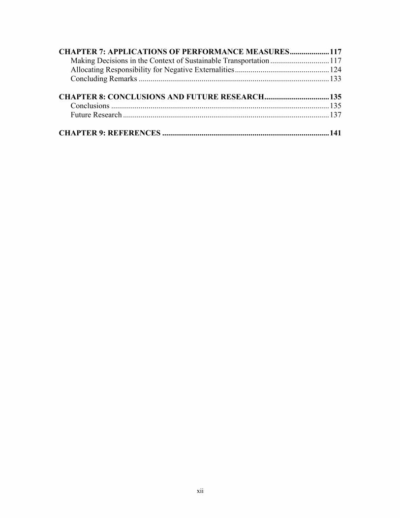
CHAPTER 7: APPLICATIONS OF PERFORMANCE MEASURES....................117   Making Decisions in the Context of Sustainable Transportation ..............................117   Allocating Responsibility for Negative Externalities................................................124   Concluding Remarks .................................................................................................133  CHAPTER 8: CONCLUSIONS AND FUTURE RESEARCH.................................135   Conclusions ...............................................................................................................135   Future Research .........................................................................................................137  CHAPTER 9: REFERENCES .....................................................................................141 

 

  xiii

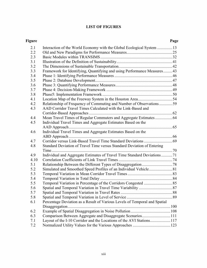
LIST OF FIGURES 

 

Figure      Page 

2.1  Interaction of the World Economy with the Global Ecological System ...............13 2.2  Old and New Paradigms for Performance Measures.............................................25 2.3  Basic Modules within TRANSIMS.......................................................................32 3.1  Illustration of the Definition of Sustainability.......................................................41 3.2  The Dimensions of Sustainable Transportation.....................................................42 3.3  Framework for Identifying, Quantifying and using Performance Measures.........43 3.4  Phase 1: Identifying Performance Measures .........................................................46 3.5  Phase 2: Database Development............................................................................47 3.6  Phase 3: Quantifying Performance Measures........................................................48 3.7  Phase 4: Decision-Making Framework .................................................................49 3.8  Phase5: Implementation Framework .....................................................................50 4.1  Location Map of the Freeway System in the Houston Area..................................54 4.2  Relationship of Frequency of Commuting and Number of Observations .............59 4.3  AAD Corridor Travel Times Calculated with the Link-Based and   Corridor-Based Approaches ..................................................................................62 4.4  Mean Travel Times of Regular Commuters and Aggregate Estimates .................64 4.5  Individual Travel Times and Aggregate Estimates Based on the  

AAD Approach......................................................................................................65 4.6  Individual Travel Times and Aggregate Estimates Based on the 

ABD Approach ......................................................................................................66 4.7  Corridor versus Link-Based Travel Time Standard Deviations ............................69 4.8  Standard Deviation of Travel Time versus Standard Deviation of Entering   Time.......................................................................................................................70 4.9  Individual and Aggregate Estimates of Travel Time Standard Deviations ...........71 4.10  Correlation Coefficients of Link Travel Times .....................................................74 5.1  Relationship Between the Different Types of Disaggregation..............................78 5.2  Simulated and Smoothed Speed Profiles of an Individual Vehicle.......................81 5.3  Temporal Variation in Mean Corridor Travel Times ............................................83 5.4  Temporal Variation in Total Delay .......................................................................84 5.5  Temporal Variation in Percentage of the Corridors Congested ............................85 5.6  Spatial and Temporal Variation in Travel Time Variability .................................87 5.7  Spatial and Temporal Variation in Travel Rates ...................................................88 5.8  Spatial and Temporal Variation in Level of Service .............................................89 6.1  Percentage Deviation as a Result of Various Levels of Temporal and Spatial   Disaggregation.....................................................................................................100 6.2  Example of Spatial Disaggregation in Noise Pollution .......................................108 6.3  Comparison Between Aggregate and Disaggregate Scenarios............................111 7.1  Layout of the I-10 Corridor and the Locations of the AVI Stations....................117 7.2  Normalized Utility Values for the Various Approaches .....................................123  

  xiv 

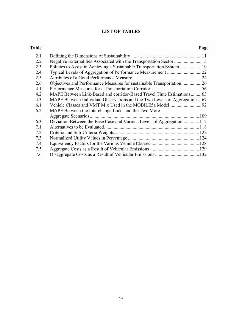
LIST OF TABLES 

 

Table       Page 

2.1  Defining the Dimensions of Sustainability............................................................11 2.2  Negative Externalities Associated with the Transportation Sector .......................13 2.3  Policies to Assist in Achieving a Sustainable Transportation System ..................19 2.4  Typical Levels of Aggregation of Performance Measurement .............................22 2.5  Attributes of a Good Performance Measure ..........................................................24 2.6  Objectives and Performance Measures for sustainable Transportation.................26 4.1  Performance Measures for a Transportation Corridor...........................................56 4.2  MAPE Between Link-Based and corridor-Based Travel Time Estimations.........63 4.3  MAPE Between Individual Observations and the Two Levels of Aggregation....67 6.1  Vehicle Classes and VMT Mix Used in the MOBILE5a Model...........................92 6.2  MAPE Between the Interchange Links and the Two More   Aggregate Scenarios ............................................................................................109 6.3  Deviation Between the Base Case and Various Levels of Aggregation..............112 7.1  Alternatives to be Evaluated................................................................................118 7.2  Criteria and Sub-Criteria Weights .......................................................................122 7.3  Normalized Utility Values in Percentage ............................................................124 7.4  Equivalency Factors for the Various Vehicle Classes.........................................128 7.5  Aggregate Costs as a Result of Vehicular Emissions..........................................129 7.6  Disaggregate Costs as a Result of Vehicular Emissions .....................................132  

 

1 

CHAPTER 1: INTRODUCTION  

BACKGROUND  Sustainable Transportation 

  Transportation is an essential social and economic activity that also results in a 

number of negative externalities, which include (1): i) air pollution; ii) noise pollution; 

iii) accidents; iv) energy use; v) congestion; vi) depletion of oil and other natural 

resources; vii) social disruption; and viii) damage of landscape and soil. These negative 

externalities are associated with all facets of the transportation lifecycle that include the 

production of vehicles, their use, and ultimately their disposal. The fact that the rate of 

the worldís motor vehicle growth is projected to outpace the worldís population growth 

is, therefore, a major concern (2). In the United States, for example, it was estimated that 

over the past twenty-five years the rate of increase in drivers was seventy-two percent 

compared to an increase in population growth of only twenty-three percent. Also, during 

the same period the rate of increase in household vehicles was estimated to be more than 

six times the rate of population growth (3). Planners and environmentalists have 

predicted that such trends will result in economic, social, and environmental needs of 

both current and future generations not being met. This challenge led to the creation of 

the concept of sustainable development. 

  The term sustainable development was introduced as early as 1980, and in 1987 the 

report by the World Commission on Environment and Development (the so-called 

Brundtland Commission) provided a definition for sustainable development that is still 

widely used (4): ì development that meets the needs of the present without compromising 

the ability of future generations to meet their own needs.î  The Presidentís Council on 

Sustainable Development, which President Clinton established in 1993, subsequently 

adopted this definition (5). Sustainable transportation can be seen as an expression of 

sustainable development in the transportation sector and it can be defined as follows (6): 

ì sustainable transportation involves infrastructure investments and travel policies that 

serve multiple goals of economic development, environmental stewardship, and social 

equity. The objective is to optimize the use of the transportation system to achieve 

  2

economic and related social and environmental goals, without sacrificing the ability of 

future generations to achieve the same goals.î  

  The concepts and principles associated with sustainable transportation are well 

documented and are supported by many decision-makers. These concepts and principles 

are related to the dimensions of sustainable development and include the improvement 

and protection of the following aspects (7): 

 

• employment; 

• efficiency; 

• livability; 

• equity; 

• safety and security; 

• accessibility; 

• mobility; 

• and environmental protection. 

 

  Although these are all laudable goals, the challenge remains to insure that they are 

implemented. Methodologies for their implementation in a consistent and comprehensive 

manner, however, are virtually nonexistent. Sustainable transportation can be considered 

as one of the most debated but least applied concepts in urban and transportation planning 

(8). 

  Many authors have investigated possible deficiencies with regard to current 

transportation planning practice and identified the following as key areas for 

improvement (8-15): i) the lack of understanding and recognition of the increasingly 

important social, economic, environmental, and public policy issues; ii) the lack of 

practical guidelines on how to address these challenges; iii) the lack of quantified 

measures so that progress can be monitored and decisions made; and iv) the lack of co-

ordination between decision-makers and other stakeholders. 

  These deficiencies can to a large extent be addressed if the concepts associated with 

sustainable transportation are clearly defined and quantified. The reality, however, is that 

the sustainability implications of transportation have not been quantified and are even 

  3

qualitatively unclear (10). The reasons why sustainable transportation has not been 

adequately quantified can be summarized as follows (13,14): 

 

• Sustainable transportation is a fairly new concept of which the objectives and 

scope of activities are unclear; 

• There is a lack of guidelines for identifying appropriate performance measures;  

• The current state of the practice in terms of modeling and planning techniques is 

too limited in its level of accuracy and detail to adequately quantify sustainable 

transportation performance measures; and 

• Even if sustainable transportation performance measures can be adequately 

quantified, it is unclear how to make trade-offs and decisions in a consistent and 

unbiased manner. 

 

Performance Measures for Sustainable Transportation 

  The first challenge, therefore, is to identify appropriate performance measures for 

sustainable transportation. Performance measures for sustainable development can be 

defined as (16) ì various statistical values that collectively measure the capacity to meet 

present and future needs as well as public policy goals and outcomes.î  Performance 

measures have a number of specific applications, but in general they are used to assist 

decision-makers in making informed decisions (17,18). 

  The importance of performance measures related to sustainable transportation has 

been widely recognized. Gardner and Carlsen state that (19) ì if we are to make good 

decisions about policy relating to sustainable transportation we need reliable 

information on the state of the environment and the factors that impact upon it.î  The 

Intermodal Surface Transportation Efficiency Act of 1991 (ISTEA) and the 

Transportation Equity Act of the 21st Century (TEA-21) make reference of performance 

measures and their use in monitoring different policies related to sustainable 

transportation (20,21). To adhere to the requirements of these pieces of legislation, 

performance measures are required to address environmental, social, and economic 

objectives in addition to the general transportation objectives. Specific criteria such as 

mobility, connectivity, accessibility, energy efficiency, air quality, noise, safety, 

  4

neighborhood impact, resource impact, and economic development will have to be 

addressed (22). 

  A number of performance measures that have historically been used for other 

purposes, such as mobility and congestion studies, can potentially be used for quantifying 

sustainable transportation. These performance measures up to now have been quantified 

with data that are aggregated over many vehicles. The researchers in this study postulated 

that the capability of modeling travel characteristics on a disaggregate level can improve 

the accuracy with which such performance measures are quantified. This is the case 

because a number of negative externalities such as vehicular emissions are inherently 

nonlinear. In these situations aggregate approximations may result in considerable error. 

More importantly, considering only averages or aggregate information can cause analysts 

to overlook a number of crucial sustainability issues. (23). 

 

Modeling Techniques for Sustainable Transportation 

  The second challenge is to adequately quantify performance measures for sustainable 

transportation. In the case of base year conditions, performance measures are mostly 

quantified with survey data, although there are a number of performance measures or 

applications for which data need to be manipulated with models. Predictions of future 

conditions are exclusively made with the aid of models. Models used for sustainable 

transportation analysis include transportation planning models, traffic simulation models, 

transportation environmental impact models, and economic models. 

  The current state of the practice in terms of transportation planning modeling is the 

so-called four-step travel demand model. This is a macroscopic approach that results in 

aggregate vehicle flows on the selected network (24). New innovations in transportation 

modeling, however, make it possible to obtain travel information at the disaggregate 

level. An example of such a model is the Transportation Analysis and Simulation System 

(TRANSIMS) model that is currently under development by the Los Alamos National 

Laboratory (25). On the data collection front, the advent of Automatic Vehicle 

Identification (AVI) has also made it possible to monitor travel characteristics on a 

disaggregate level (23). Transportation environmental impact models include air 

  5

pollution models, noise pollution models, and energy consumption models. Economic 

models are used to determine the economic implications of transportation. 

 

Decision-Making for Sustainable Transportation 

  The third challenge is to use performance measures for measurement and decision-

making in the context of sustainable transportation. Because the transportation system is 

comprised of a complex system with conflicting economic and environmental objectives, 

it is necessary to use a decision-making technique that can consider the multiple and 

conflicting objectives (26). Single-objective decision-making techniques such as benefit-

cost analysis (which is based on monetary values) are not adequate to deal with the 

complexities associated with sustainable transportation (27). Various multi-criteria 

decision-making techniques have been developed to deal with this complex problem. 

 

STATEMENT OF THE PROBLEM 

  The actual implementation of sustainable transportation concepts up to now have 

been very disappointing, and successes are few and far between (28). The reason for this 

is that the concept of sustainable transportation is still unclear and it has not been 

adequately quantified. There is, therefore, a need to clearly define sustainable 

transportation and to show how performance measures can assist in quantifying it. 

  Because sustainability requires a more integrated view of the world, traditional 

performance measures that just look at specific transportation related aspects are often 

not very useful as indicators for sustainable transportation (29). The challenge is to assess 

the outcomes of transportation programs and policies in terms of the broader 

sustainability goals of economic, social, and environmental sustainability. There is a 

myriad of possible indicators that can fall into the realm of sustainable transportation 

(30). The selection of appropriate performance measures is very important because they 

direct the focus of planners and decision-makers. Because a poor selection of 

performance measures can lead to poor decisions and outcomes, there is a need to 

propose an approach for identifying appropriate performance measures for sustainable 

transportation (30,31). 

  6

  Decision-makers need accurate information on performance measures to be able to 

make informed decisions. Some of these performance measures can be quantified on an 

aggregate level, whereas others can only be accurately quantified on a disaggregate level. 

Performance measures for sustainable transportation based on disaggregate data currently 

are virtually nonexistent. This is because, until recently, there has been a lack of adequate 

data, tools, and techniques to quantify performance measures at a disaggregate level (32). 

The latest state-of-the-art transportation simulation models and data collection 

techniques, however, are able to provide travel-related information at a disaggregate 

level. There is, therefore, a need to develop procedures with the latest transportation 

modeling and data collection techniques to quantify additional performance measures and 

to improve the accuracy with which some existing performance measures are quantified. 

  The process by which alternatives are to be formulated, evaluated, and selected is 

becoming more constrained in terms of required procedures and outputs (33). Multi-

criteria decision-making techniques have the potential to deal with the complexities 

associated with sustainable transportation (27). It is, therefore, necessary to investigate 

existing multi-criteria decision-making techniques to determine whether they are suitable 

for dealing with the decision-making problems regarding sustainable transportation, and 

to propose a suitable technique. 

 

RESEARCH OBJECTIVES 

  This research begins with the hypothesis that the accuracy with which performance 

measures for sustainable transportation are quantified can be improved by quantifying 

such measures on a more disaggregate level. The objective of this research is to develop 

and apply a methodology through which disaggregate travel information can be used to 

supplement traditional aggregate travel information in quantifying performance measures 

for sustainable transportation and to use such quantified measures in the decision-making 

process. The research will focus on the following elements: 

 

• To define sustainable transportation and propose a mechanism for identifying 

appropriate performance measures for sustainable transportation; 

  7

• To use AVI data and the state-of-the-art in transportation simulation models to 

quantify travel related performance measures at aggregate and disaggregate 

levels; 

• To use traffic simulation models and environmental impact models to quantify 

environmental related sustainable transportation performance measures;  

• To conduct various comparisons between the aggregate and disaggregate 

approaches; and 

• To illustrate the application of sustainable transportation performance measures 

through the use of a multi-criteria decision-making technique and the allocation of 

responsibility through equivalency factors. 

 

  The scope of the research will be such that the methodologies that are developed will 

be of a generic nature that can be applied at both the local and network-wide levels, as 

well as for a wide range of sustainable transportation performance measures. The 

applications, however, will focus on mobility and environmental related performance 

measures for freeway corridors. 

 

CONTRIBUTION OF THE RESEARCH 

  Performance  measures  for  sustainable  transportation  up  to  now  have  only  been 

quantified in very limited cases. Even when such measures have been quantified, it was 

based  on  aggregate  datasets.  This  research  will  illustrate  how  to  obtain  disaggregate 

travel  information  and  use  it  to  improve  quantification  of  performance measures  for 

sustainable transportation. The following are some of the individual contributions of the 

research:  i)  sustainable  transportation  is  defined  and  a  framework  is  proposed  for 

identifying,  quantifying,  and  using  performance  measures  in  the  decision-making 

process; ii) the shortcomings of the current aggregate-based practice and the benefits of 

the  proposed  methodology  for  quantifying  performance  measures  for  sustainable 

transportation at a disaggregate level are demonstrated; and iii) a methodology for using 

performance measures  for  sustainable  transportation  in  the  decision-making  process  is 

proposed. 

 

  8

ORGANIZATION OF THE REPORT 

  The report has been divided into eight chapters. Chapter 1 includes an introduction to 

the research and covers aspects such as background, statement of the problem, research 

objectives, methodology, contribution of the research, and organization of the report. 

Chapter 2 provides a literature review of the state of the art of the main topics of this 

research. It includes a review of sustainable transportation, legislative and policy 

frameworks, performance measures for sustainable transportation, modeling techniques, 

and decision-making for sustainable transportation. 

  Chapter 3 provides a framework for achieving sustainable transportation. It contains a 

proposed definition for sustainable transportation, the decision-making process for 

sustainable transportation, and some candidate performance measures. Chapter 4 contains 

an illustration on how travel time and travel time variability can be quantified at various 

levels of aggregation by using AVI data. Chapter 5 illustrates how a wide range of 

mobility related performance measures can be quantified at various levels of aggregation 

by using a transportation planning model, TRANSIMS. 

  Chapter 6 illustrates how environmental related performance measures such as 

vehicular emission, noise pollution, and fuel consumption can be quantified at various 

levels of aggregation by using a traffic simulation model and environmental models. The 

implication of quantifying all the above-mentioned performance measures at the various 

levels of aggregation is discussed. Chapter 7 includes two applications of performance 

measures for sustainable transportation, namely: using performance measures in a multi-

criteria decision-making technique; and allocating responsibility to motorists for 

generating negative externalities. 

  Chapter 8 contains the conclusions and a proposal for future research. 

  9

CHAPTER 2: LITERATURE REVIEW  

  In Chapter 1 this report identified a number of needs that have to be addressed in 

order to ensure the effective and efficient implementation of the concepts of sustainable 

transportation. This chapter contains a literature review on the state of the practice with 

respect to identifying and addressing these needs. The main focus areas of the literature 

review are: sustainable transportation; legislative, planning, and policy frameworks; 

performance measures; and modeling techniques. 

 

SUSTAINABLE TRANSPORTATION Evolution of the Concept of Sustainable Transportation 

  In order to obtain a thorough understanding of the concept of sustainable 

transportation it is instructive to explore its evolution. While the term sustainable 

development is fairly recent, some principles associated with it date back to the 

eighteenth century economist and philosopher Thomas Malthus. He theorized that 

temporary improvements in human living standards would trigger population surges, 

which would outpace technological growth and resource availability (34). These theories 

were rekindled during the early 1960s when there was a growing concern over the human 

impact on the environment (2). In the 1970s scientists identified some specific concerns 

such as global warming, acid rain, depletion of the ozone layer, excessive population 

growth, loss of tropical forests, and biological diversity (2). The term sustainable 

development was first used by the World Conservation Strategy (WCS) in 1980. They 

stressed the interdependence of conservation and development and emphasized that 

humanity is part of nature and has no future unless people conserve nature and natural 

resources (2). 

  In 1987 the report by the World Commission on Environment and Development (the 

so-called Brundtland Commission) re-emphasized the importance of sustainable 

development and provided the widely used definition for sustainable development, as 

included in Chapter 1 (4). The United Nations Conference on Environment and 

Development (UNCED), which was held in Rio de Janeiro in 1992, gave the concept of 

  10

sustainable development the status of a global mission through the adoption of the so-

called Agenda 21 (35). 

  The momentum for achieving sustainable development accelerated during the 1990s 

and there are currently numerous initiatives of sustainable development across the world, 

particularly in Europe, Canada, and the United States. Important initiatives in the United 

States include the Presidentís Council on Sustainable Development and the Livability 

Agenda of the President and Vice President. The mandate of the Presidentís Council on 

Sustainable Development is to advise the president on key sustainability issues (5). The 

Livability Agenda focuses on strengthening the Federal role in support of state and local 

efforts to build livable communities for the twenty-first century (36). 

 

Definitions for Sustainable Development and Sustainable Transportation 

  The concept of sustainability has been much debated and argued over. A number of 

authors have provided definitions for sustainable development and sustainable 

transportation (4,17,37-42). The definitions for sustainable development are fairly wide 

ranging although they all include some type of reference to intergenerational equity, 

where the goal is to ensure a quality environment for current and future generations. 

Sustainability, therefore, refers to long-term availability of adequate resources that are 

necessary for the achievement of pre-specified goals. Development and growth should 

also be maintained within the ecological boundaries and should not extend beyond the 

carrying capacity of the natural environment. Sustainable development is, therefore, a 

dynamic concept that takes into consideration the expanding needs of a growing world 

population, including its entire social, economic, ecological, geographic, and cultural 

dimensions (28). It should also be noted that the concept of sustainability should be 

viewed as a continuum, representing varying degrees of sustainability and 

unsustainability (2). 

  Sustainable transportation is an expression of sustainable development in the 

transportation sector. The challenge is to make transportation sustainable by addressing 

its consumptive nature of renewable and non-renewable resources, as well as its 

environmental impacts. Large institutions such as the World Bank and the Organization 

for Economic Co-operation and Development (OECD), as well as various other authors 

  11

have provided definitions for sustainable transportation (6,17,32,35,39,42,43,44). These 

definitions are all based on the broader concept of sustainable development and are 

concerned with meeting current and future mobility and accessibility needs without 

resulting in undue negative externalities. Table 2.1 is a description of what is understood 

with each of the dimensions of sustainability (7,17). 

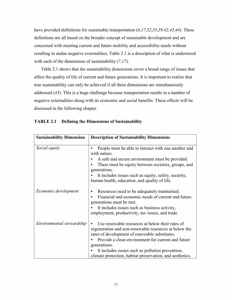
  Table 2.1 shows that the sustainability dimensions cover a broad range of issues that 

affect the quality of life of current and future generations. It is important to realize that 

true sustainability can only be achieved if all three dimensions are simultaneously 

addressed (43). This is a huge challenge because transportation results in a number of 

negative externalities along with its economic and social benefits. These effects will be 

discussed in the following chapter. 

 TABLE 2.1  Defining the Dimensions of Sustainability  

Sustainability Dimension  

Description of Sustainability Dimensions 

Social equity  

• People must be able to interact with one another and with nature. • A safe and secure environment must be provided. • There must be equity between societies, groups, and generations. • It includes issues such as equity, safety, security, human health, education, and quality of life.  

Economic development  

• Resources need to be adequately maintained. • Financial and economic needs of current and future generations must be met. • It includes issues such as business activity, employment, productivity, tax issues, and trade.  

Environmental stewardship  • Use renewable resources at below their rates of regeneration and non-renewable resources at below the rates of development of renewable substitutes. • Provide a clean environment for current and future generations. • It includes issues such as pollution prevention, climate protection, habitat preservation, and aesthetics. 

 

  12

Negative Externalities 

  The economic system takes renewable and non-renewable resources from the 

environment, processes them to derive some benefits and then discards what is left as 

different forms of waste into the environment. The only continuous external input into the 

global system is solar energy, and the only output leaving the system is low-level heat. 

The dumping of waste streams may lead to substantial and sometimes irreversible 

damage to the environment. The interests of future generations are damaged: if non- 

renewable resources are used without enabling the production of full substitutes; if 

renewable resources are used faster than they can be reproduced; or if more waste is 

dumped into the environment than the ecological systems can safely absorb (45). 

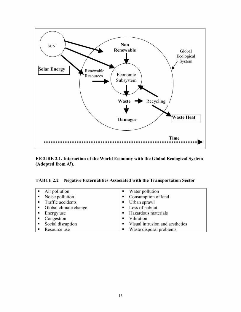
  Figure 2.1 shows how the world economy interacts with the global ecological 

subsystem. In this figure the economic subsystem is represented as the inner circle in the 

diagram and the global ecological system as the outer circle. In an unsustainable situation 

the size of the economic subsystem continues to increase up to a point that the ecological 

system is not able to accommodate it anymore (45). Transportation plays a key role in the 

economic system and, therefore, has a major impact on the ecological system. Results 

showed that transportation can typically represent ten percent of a nationís gross 

domestic product and is responsible for twenty-two percent of the global energy 

consumption and twenty-five percent of fossil fuel burning across the world (2,46). Table 

2.2 provides a brief description of each of the negative externalities associated with 

transportation. 

  13

 

FIGURE 2.1. Interaction of the World Economy with the Global Ecological System (Adopted from 45).   TABLE 2.2  Negative Externalities Associated with the Transportation Sector   Air pollution  Noise pollution  Traffic accidents  Global climate change  Energy use  Congestion  Social disruption  Resource use 

Water pollution  Consumption of land  Urban sprawl  Loss of habitat  Hazardous materials  Vibration  Visual intrusion and aesthetics  Waste disposal problems 

 

 

 SUN 

Economic Subsystem 

Non Renewable 

 Renewable  Resources 

Waste

Damages

Recycling 

Waste Heat 

Solar Energy 

Time 

Global Ecological System 

  14

LEGISLATIVE, PLANNING, AND POLICY FRAMEWORKS Legislative Framework 

  Legislation forms the basis for transportation planning practice. It is, therefore, 

necessary to understand the relevant legislation when attempting to plan for a sustainable 

transportation system. The following are Federal laws in the United States that can have 

an affect on sustainable transportation (47): 

 

• Urban Mass Transportation Act of 1964; 

• National Historic Preservation Act of 1966; 

• Department of Transportation Act of 1966; 

• Housing and Urban Development Act of 1966; 

• National Environmental Policy Act of 1969; 

• Noise Control Act of 1972; 

• Federal Aid to Highways Act (Various years); 

• Clean Water Act (with major amendments in 1972, 1977, and 1987); 

• Clean Air Act (with major amendments in 1965, 1970, 1977, and 1990); 

• Oil Pollution Act of 1990; 

• Intermodal Surface Transportation Efficiency Act (1991); 

• Energy Policy Act (1992); and  

• Transportation Equity Act of the 21st Century (1997). 

 

  The watershed legislation in terms of transportation planning in the United States was 

the Intermodal Surface Transportation Efficiency Act of 1991. This act implicitly 

supports the goals of sustainable transportation, and its three-part philosophy is stated as: 

i) decentralization; ii) friendlier to the environment; and iii) more responsive to the needs 

of increasingly diverse populations and businesses (48). This philosophy can be achieved 

by promoting transportation systems that maximize mobility and accessibility and 

minimize transportation related negative externalities. The Transportation Equity Act for 

the 21st Century, which builds on the initiatives of ISTEA, was signed into law in June 

1998. Some of the significant features of TEA-21 include: i) a guaranteed level of 

Federal funds for surface transportation through fiscal year 2003; ii) extension of the 

  15

Disadvantaged Business Enterprises (DBE) program; iii) strengthening of the safety 

programs; iv) continuation of the highways and transit initiatives under ISTEA; and v) 

investing in research and its application to maximize the performance of the 

transportation system (21). Apart from these pieces of legislation, the Clean Air Act 

Amendments (CAAA) of 1990 and the National Environmental Policy Act (NEPA) 

process ensure that air pollution associated with transportation is addressed (20). 

 

Planning Framework 

  ISTEA and TEA-21 also outline transportation planning requirements of state 

departments of transportation and metropolitan planning organizations (MPOs). These 

requirements must be followed in order for these levels of government to receive Federal 

funding for transportation projects. Metropolitan areas are required to develop long-term 

(twenty-year) Metropolitan Transportation Plans (MTPs) and short-term (three-year) 

Transportation Improvement Plans (TIPs). The metropolitan areas provide their TIPs to 

the state so that it can prepare a Statewide Transportation Improvement Plan (STIP) (14). 

Where the planning process identifies a problem in a corridor or sub-area that suggests 

the possible need for a major investment using Federal funds, a Major Investment Study 

(MIS) may be required. The purpose of a MIS is to analyze solutions to address 

substantial transportation problems and to present this information to decision-makers 

(20). 

  The NEPA process focuses on projects after they have been included in the MTP or 

TIP. This process can be performed in conjunction or at the end of a MIS. There are three 

classes of action that prescribe the level of documentation required in the NEPA process. 

These actions relate to the type of transportation investments and their anticipated 

impacts on the environment, and can be summarized as follows (20): 

 

• Class I: Environmental Impact Statement: These are actions that significantly 

affect the environment and require an Environmental Impact Statement (EIS). 

• Class II: Categorical Exclusions: These are actions that do not have a significant 

effect and are excluded from the requirements to prepare environmental 

assessments. 

  16

• Class III: Environmental Assessment: These are actions in which the significance 

of the environmental impact is not clearly established. An Environmental 

Assessment (EA) needs to be prepared to determine the appropriate 

environmental document required. 

 

  The Clean Air Act Amendments of 1990 set forth specific air quality goals to be 

achieved by certain dates. Once an area reaches attainment, it is classified as a 

maintenance area for twenty years past the attainment date and must still fulfill CAAA 

requirements. The United States Environmental Protection Agency (EPA) is the Federal 

agency charged with implementing the CAAA. The EPA established National Ambient 

Air Quality Standards (NAAQS) in 1970, with the purpose of protecting human life. In 

terms of the NAAQS the EPA has set national air quality standards for six principal 

pollutants, namely CO, lead, NOx, ozone, particulate matter and SO2. The CAAA require 

that the EPA review the NAAQS every five years to determine if the standards are still 

adequate. The EPA relies on the states for preparing State Implementation Plans (SIPs) to 

submit to the EPA, detailing how they intend to reduce vehicular emissions (49). 

  If the EPA classifies an area as non-attainment for air quality, those transportation 

plans and programs must conform to air quality goals or Federal funding may be 

withheld. The plans demonstrate conformity if the planís forecasted emission estimates 

are less than or equal to that areaís on-road Motor Vehicle Emissions Budget (MVEB) 

listed in the SIP. A MVEB is generally required for each transportation related pollutant 

and/or pollutant precursor for which the area is in non-attainment. If a non-attainment 

area cannot demonstrate conformity within the required timeframe, a transportation 

conformity lapse occurs. During such a lapse, the EPA allows only certain transportation 

projects to proceed. Conformity determination must be performed each time a SIP is 

revised that adds, deletes, or changes emission budgets, or when Transportation Control 

Measures (TCMs) are submitted to the EPA, detailing how those reductions will occur 

(49). 

  ISTEA requires non-attainment area MTPs to be reviewed and updated at least every 

three years, whereas TIPs in non-attainment areas must be updated at least every two 

years. The CAAA state that conformity to a SIP means conformity to the planís purpose 

  17

of eliminating or reducing the severity and number of violations of the NAAQS. In 

addition, the activities must not cause or contribute to a new violation, increase the 

frequency or severity of an existing violation, or delay timely attainment of any standard 

interim milestone (50). 

  The procedure of showing that the transportation plans, programs and projects are 

conforming to air quality goals is a long and detailed process that requires many skilled 

personnel and a sizable budget. It is, however, a very necessary process to assist in 

achieving sustainable transportation. Failure to adhere to the CAAA and the 

ISTEA/TEA-21 requirements can have serious consequences, both due to Federally 

imposed sanctions in the form of funding that is withheld, as well as all the negative 

effects related to poor air quality. 

 

Policy Framework 

  As in the case of legislation, policies can play a pivotal role in achieving the goals of 

sustainable transportation. The concept of policy may be defined as (51) ì a purposeful 

course of action followed by an actor or set of actors in dealing with a problem or matter 

of concern.î  This definition of policy links it to a goal oriented action rather than to 

random behavior or chance occurrences. Public policies are those developed by 

governmental bodies, and they are designed to accomplish specified goals or produce 

definite results (51). Because policies are linked to goals, they can be developed as part 

of a strategic planning exercise. The transportation sector is, however, a particularly 

difficult sector to address due to its high dependence on fossil fuels and the fact that 

objectives associated with an effective and efficient transportation system are often not 

compatible with environmental objectives (52). The development of appropriate policy 

for transportation is, therefore, a complex issue. 

  The main focus of a policy for sustainable transportation should be to achieve long-

term sustainability based on the understanding that the world economy is a sub-system of 

the global ecological system, which is restricted by its capacity (45). The World Bank 

defines a policy for sustainable transportation as follows (39): ì it identifies and 

implements the win-win policy instruments and explicitly confronts the tradeoffs so that 

the balance is chosen rather than accidentally arrived at. It is a policy of informed, 

  18

conscious choices.î  A number of authors have investigated policy options to support 

sustainable transportation. The following are some of the most important policy 

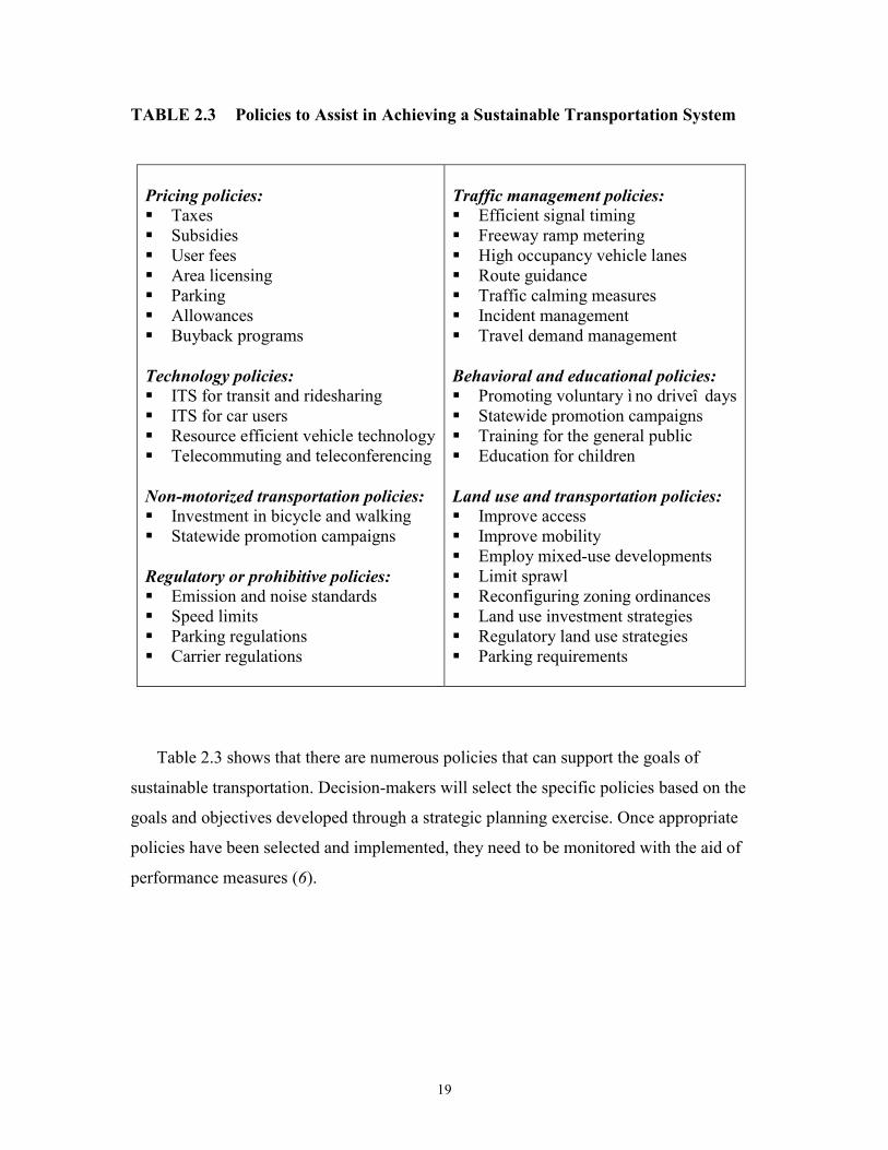
categories that can be used in the context of sustainable transportation, whereas Table 2.3 

shows a detailed listing of the specific policies that can be utilized under each category 

(17,28,43,53,54,55): 

 

• Pricing policies: Transportation systems and services must be priced to result in 

the optimal allocation of resources. This entails the inclusion of external social 

costs into the pricing of transportation. 

• Technology policies: Technology plays a vital role in providing transportation 

options, making information available to users, and reducing environmental 

damage. 

• Non-motorized transportation policies: Among the different modes of 

transportation, walking and cycling rank highest on the sustainability scale, and 

the single-occupant automobile ranks the lowest. It is, therefore, necessary to have 

policies in place that promote the utilization of non-motorized modes of 

transportation. 

• Regulatory or prohibitive policies: In some instances it is necessary to regulate 

and prohibit certain actions. 

• Traffic management policies: Traffic flow conditions can be improved through a 

number of traffic management techniques, and improved traffic flow can assist in 

making transportation more sustainable. 

• Behavioral and educational policies: Users of the transportation system need to 

change their transportation behavior in order to facilitate the achievement of a 

more sustainable transportation system. 

• Land use and transportation policies: Without adequate land use reforms and an 

integrated land use and transportation approach, the goals of sustainable 

transportation are not likely to be met. 

  19

TABLE 2.3  Policies to Assist in Achieving a Sustainable Transportation System  

 Pricing policies:  Taxes  Subsidies  User fees  Area licensing  Parking  Allowances  Buyback programs  Technology policies:  ITS for transit and ridesharing  ITS for car users  Resource efficient vehicle technology  Telecommuting and teleconferencing  Non-motorized transportation policies:  Investment in bicycle and walking  Statewide promotion campaigns  Regulatory or prohibitive policies:  Emission and noise standards  Speed limits  Parking regulations  Carrier regulations  

 Traffic management policies:  Efficient signal timing  Freeway ramp metering  High occupancy vehicle lanes  Route guidance  Traffic calming measures  Incident management  Travel demand management  Behavioral and educational policies:  Promoting voluntary ì no driveî  days  Statewide promotion campaigns  Training for the general public  Education for children  Land use and transportation policies:  Improve access  Improve mobility  Employ mixed-use developments  Limit sprawl  Reconfiguring zoning ordinances  Land use investment strategies  Regulatory land use strategies  Parking requirements 

 

 

  Table 2.3 shows that there are numerous policies that can support the goals of 

sustainable transportation. Decision-makers will select the specific policies based on the 

goals and objectives developed through a strategic planning exercise. Once appropriate 

policies have been selected and implemented, they need to be monitored with the aid of 

performance measures (6). 

 

  20

PERFORMANCE MEASURES The Role of Performance Measures 

  Performance measures or indicators are very important in the context of sustainable 

development and sustainable transportation. Agenda 21 of the United Nations Conference 

on Environment and Development considers the function of performance measures as 

follows (56): ì indicators of sustainable development need to be developed to provide 

solid bases for decision-making at all levels and to contribute to a self-regulating 

sustainability of integrated environment and development systems.î  Performance 

measures are broadly used for simplification, quantification, and communication. They 

are able to translate data and statistics into succinct information that can be readily 

understood and used by several groups of people including scientists, administrators, 

politicians, and the general public (57,58). A comprehensive performance measure would 

include measurements of the condition, trends over time, and the share attributed to the 

different agencies and/or actors (56). 

  ISTEA and TEA-21 recognize performance monitoring as a critical part of 

transportation planning and have called for a more performance-based approach. This 

requires that the performance of transportation systems must be quantitatively measured 

for a variety of modes and criteria (22). Apart from the requirements of legislation, 

performance measures can be very powerful planning and management tools. The 

following are some of the most important uses of performance measures (31,59): provide 

a broad perspective; assess facility or system performance; calibrate models; identify 

problems; develop and assess improvements; formulate programs and priorities; educate 

a wide range of interest groups; and set policies. Although performance measures have a 

wide range of applications, there are instances where they should not be used, such as to 

(59): isolate the effects of individual regulations; provide a full economic analysis; define 

acceptable levels of impact; and set final priorities. Performance measures are, therefore, 

able to provide the decision-maker with the quantitative information necessary to make 

informed decisions. 

 

  21

Levels of Aggregation 

  Performance measures are quantified with information that is prepared from various 

data sources. The quantified performance measures can be aggregated and weighted in 

order to produce composite measures known as indices (56). Indices are often used to 

measure trends and to track progress toward a goal. They have been developed for a 

number of applications such as for infrastructure conditions and congestion. The 

advantages of indices are as follows (60): 

 

• Easy to use;  

• Simple to interpret; and 

• Ability to reduce information overloads that can often result from individual 

performance measures. 

 

  The problems with indices, however, are as follows (44): 

 

• Can mask information;  

• Their robustness can be limited by different spatial and temporal scales; and 

• It is not always clear how and by whom the indices were developed.  

 

  Very few authors have looked into indices for sustainable transportation. Litman 

proposes a sustainable transportation index that is based on fourteen performance 

measures that range from personal travel characteristics to transportation system 

performance (29). Black proposes an index that is based on principal component analysis 

and that uses the following measures (61): 

 

• Dependence on petroleum fuels; 

• Impact of emissions on local air quality and human health; 

• Number of injuries and fatalities due to road accidents; 

• The effect of congestion; and 

• Availability of other modes. 

  22

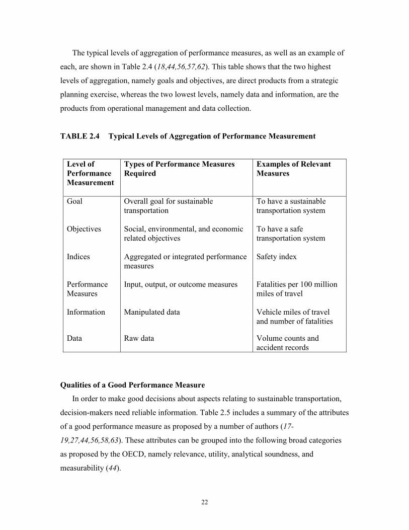
  The typical levels of aggregation of performance measures, as well as an example of 

each, are shown in Table 2.4 (18,44,56,57,62). This table shows that the two highest 

levels of aggregation, namely goals and objectives, are direct products from a strategic 

planning exercise, whereas the two lowest levels, namely data and information, are the 

products from operational management and data collection. 

 

TABLE 2.4  Typical Levels of Aggregation of Performance Measurement 

 

Level of Performance Measurement  

Types of Performance Measures Required 

Examples of Relevant Measures 

Goal  

Overall goal for sustainable transportation  

To have a sustainable transportation system 

Objectives   

Social, environmental, and economic related objectives 

To have a safe transportation system  

Indices   

Aggregated or integrated performance measures 

Safety index 

Performance  Measures  

Input, output, or outcome measures  Fatalities per 100 million miles of travel 

Information  

Manipulated data   Vehicle miles of travel and number of fatalities  

Data  Raw data  Volume counts and accident records 

 

 

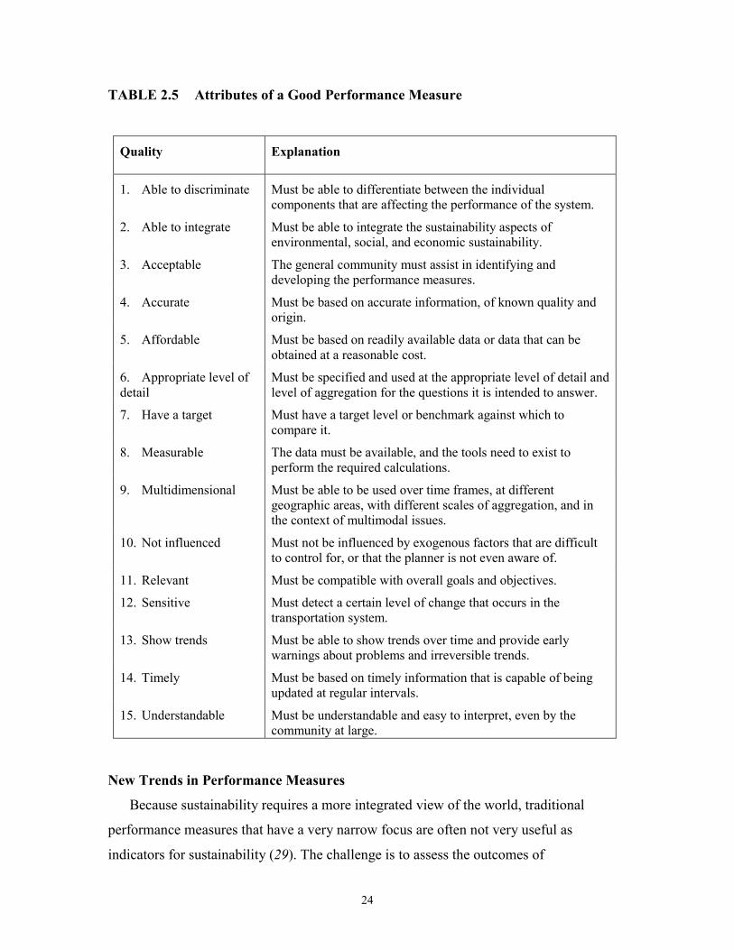
Qualities of a Good Performance Measure 

  In order to make good decisions about aspects relating to sustainable transportation, 

decision-makers need reliable information. Table 2.5 includes a summary of the attributes 

of a good performance measure as proposed by a number of authors (17-

19,27,44,56,58,63). These attributes can be grouped into the following broad categories 

as proposed by the OECD, namely relevance, utility, analytical soundness, and 

measurability (44). 

  23

  It should be noted that the fifteen attributes of a good performance measure as 

suggested in Table 2.5 are in effect a wish-list for which the planner strives. It will be 

very rare for a performance measure to possess most of the attributes listed in Table 2.5. 

There are instances where certain attributes of a good performance measure are not 

compatible and a particular performance measure will, therefore, not comply with both 

such characteristics. As an example, it is very difficult for a performance measure to be 

simple (understandable at the community level) and also able to address certain complex 

multidimensional aspects. It is often necessary, therefore, to have a variety of indicators 

for different applications. 

 

  24

TABLE 2.5  Attributes of a Good Performance Measure 

 

Quality  

Explanation 

1.  Able to discriminate  Must be able to differentiate between the individual components that are affecting the performance of the system. 

2.  Able to integrate  Must be able to integrate the sustainability aspects of environmental, social, and economic sustainability. 

3.  Acceptable  The general community must assist in identifying and developing the performance measures. 

4.  Accurate  Must be based on accurate information, of known quality and origin. 

5.  Affordable  Must be based on readily available data or data that can be obtained at a reasonable cost. 

6.  Appropriate level of detail 

Must be specified and used at the appropriate level of detail and level of aggregation for the questions it is intended to answer. 

7.  Have a target  Must have a target level or benchmark against which to compare it. 

8.  Measurable  The data must be available, and the tools need to exist to perform the required calculations. 

9.  Multidimensional  Must be able to be used over time frames, at different geographic areas, with different scales of aggregation, and in the context of multimodal issues. 

10. Not influenced  Must not be influenced by exogenous factors that are difficult to control for, or that the planner is not even aware of. 

11. Relevant  Must be compatible with overall goals and objectives. 

12. Sensitive  Must detect a certain level of change that occurs in the transportation system. 

13. Show trends  Must be able to show trends over time and provide early warnings about problems and irreversible trends. 

14. Timely  Must be based on timely information that is capable of being updated at regular intervals. 

15. Understandable  Must be understandable and easy to interpret, even by the community at large. 

  New Trends in Performance Measures 

  Because sustainability requires a more integrated view of the world, traditional 

performance measures that have a very narrow focus are often not very useful as 

indicators for sustainability (29). The challenge is to assess the outcomes of 

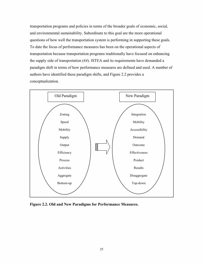
  25

transportation programs and policies in terms of the broader goals of economic, social, 

and environmental sustainability. Subordinate to this goal are the more operational 

questions of how well the transportation system is performing in supporting these goals. 

To date the focus of performance measures has been on the operational aspects of 

transportation because transportation programs traditionally have focused on enhancing 

the supply side of transportation (64). ISTEA and its requirements have demanded a 

paradigm shift in terms of how performance measures are defined and used. A number of 

authors have identified these paradigm shifts, and Figure 2.2 provides a 

conceptualization.  

 Figure 2.2. Old and New Paradigms for Performance Measures.  

 

Integration 

Mobility 

Accessibility 

Demand 

Outcome 

Effectiveness

Product 

Results 

Disaggregate 

Top-down 

Old Paradigm 

Zoning 

Speed 

Mobility 

Supply 

Output 

Efficiency 

Process 

Activities 

Aggregate  

Bottom-up 

New Paradigm 

  26

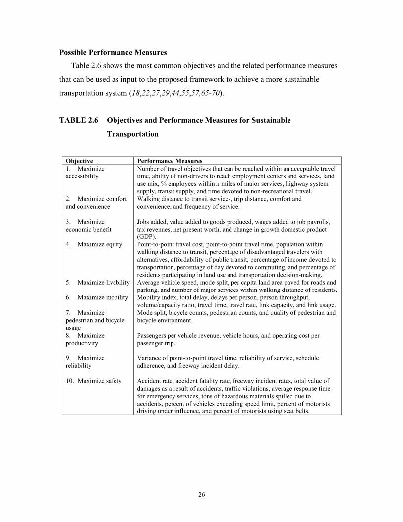
Possible Performance Measures 

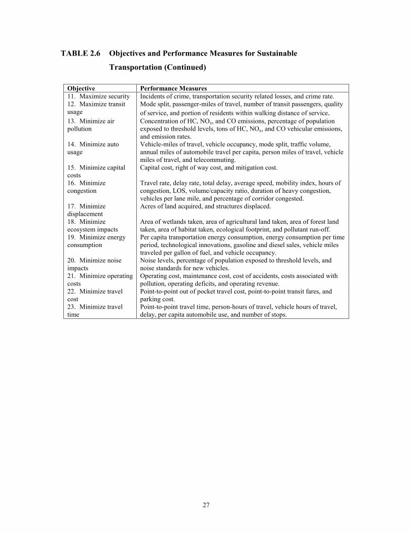
  Table 2.6 shows the most common objectives and the related performance measures 

that can be used as input to the proposed framework to achieve a more sustainable 

transportation system (18,22,27,29,44,55,57,65-70). 

 

TABLE 2.6  Objectives and Performance Measures for Sustainable 

        Transportation 

 Objective  Performance Measures 1.  Maximize accessibility 

Number of travel objectives that can be reached within an acceptable travel time, ability of non-drivers to reach employment centers and services, land use mix, % employees within x miles of major services, highway system supply, transit supply, and time devoted to non-recreational travel. 

2.  Maximize comfort and convenience  

Walking distance to transit services, trip distance, comfort and convenience, and frequency of service. 

3.  Maximize economic benefit  

Jobs added, value added to goods produced, wages added to job payrolls, tax revenues, net present worth, and change in growth domestic product (GDP). 

4.  Maximize equity    

Point-to-point travel cost, point-to-point travel time, population within walking distance to transit, percentage of disadvantaged travelers with alternatives, affordability of public transit, percentage of income devoted to transportation, percentage of day devoted to commuting, and percentage of residents participating in land use and transportation decision-making.  

5.  Maximize livability  

Average vehicle speed, mode split, per capita land area paved for roads and parking, and number of major services within walking distance of residents.  

6.  Maximize mobility  

Mobility index, total delay, delays per person, person throughput, volume/capacity ratio, travel time, travel rate, link capacity, and link usage. 

7.  Maximize pedestrian and bicycle usage  

Mode split, bicycle counts, pedestrian counts, and quality of pedestrian and bicycle environment.  

8.  Maximize productivity  

Passengers per vehicle revenue, vehicle hours, and operating cost per passenger trip. 

9.  Maximize reliability  

Variance of point-to-point travel time, reliability of service, schedule adherence, and freeway incident delay. 

10.  Maximize safety    

Accident rate, accident fatality rate, freeway incident rates, total value of damages as a result of accidents, traffic violations, average response time for emergency services, tons of hazardous materials spilled due to accidents, percent of vehicles exceeding speed limit, percent of motorists driving under influence, and percent of motorists using seat belts. 

 

  27

TABLE 2.6  Objectives and Performance Measures for Sustainable 

        Transportation (Continued)  Objective  Performance Measures 11.  Maximize security  Incidents of crime, transportation security related losses, and crime rate. 12.  Maximize transit usage 

Mode split, passenger-miles of travel, number of transit passengers, quality of service, and portion of residents within walking distance of service. 

13.  Minimize air pollution 

Concentration of HC, NOx, and CO emissions, percentage of population exposed to threshold levels, tons of HC, NOx, and CO vehicular emissions, and emission rates. 

14.  Minimize auto usage 

Vehicle-miles of travel, vehicle occupancy, mode split, traffic volume, annual miles of automobile travel per capita, person miles of travel, vehicle miles of travel, and telecommuting. 

15.  Minimize capital costs 

Capital cost, right of way cost, and mitigation cost. 

16.  Minimize congestion 

Travel rate, delay rate, total delay, average speed, mobility index, hours of congestion, LOS, volume/capacity ratio, duration of heavy congestion, vehicles per lane mile, and percentage of corridor congested. 

17.  Minimize displacement 

Acres of land acquired, and structures displaced. 

18.  Minimize ecosystem impacts 

Area of wetlands taken, area of agricultural land taken, area of forest land taken, area of habitat taken, ecological footprint, and pollutant run-off. 

19.  Minimize energy consumption 

Per capita transportation energy consumption, energy consumption per time period, technological innovations, gasoline and diesel sales, vehicle miles traveled per gallon of fuel, and vehicle occupancy. 

20.  Minimize noise impacts 

Noise levels, percentage of population exposed to threshold levels, and noise standards for new vehicles. 

21.  Minimize operating costs 

Operating cost, maintenance cost, cost of accidents, costs associated with pollution, operating deficits, and operating revenue. 

22.  Minimize travel cost 

Point-to-point out of pocket travel cost, point-to-point transit fares, and parking cost. 

23.  Minimize travel time 

Point-to-point travel time, person-hours of travel, vehicle hours of travel, delay, per capita automobile use, and number of stops. 

 

  28

MODELING TECHNIQUES   Once the appropriate performance measures have been identified, modeling 

techniques are often used to quantify such measures over space and time (17). Models for 

quantifying sustainable transportation include transportation models, transportation 

environmental impact models, and economic models. In addition to output from the 

various models, data collected through Intelligent Transportation Systems (ITS) 

applications can be used to quantify performance measures for sustainable transportation. 

The following is a discussion of aggregate and disaggregate approaches to modeling, as 

well as the appropriate data collection and modeling techniques for quantifying 

performance measures for sustainable transportation. 

 

Aggregate versus Disaggregate Approaches 

  The travel behavior of large groups is the manifestation of the travel choices of 

numerous individual travelers. Disaggregate travel models are constructed by using data 

at the level of the individual traveler, whereas with aggregate models the individuals are 

placed into groups with common characteristics. The data that are based on the group are 

an aggregate representation of the real underlying distribution of the individual data (71). 

The axioms of disaggregate behavioral modeling are that individuals represent the basic 

decision-making unit and that individuals will choose one alternative among those 

available that they find most desirable or useful. The choice depends on the attributes of 

the alternative and the socioeconomic characteristics of the individual (72). 

  The probability of a decision is considered to be a function of the utility for that 

decision (73). For modeling purposes the utility is composed of two components, namely 

the observed attributes referred to as the representative utility, and an unobserved 

component known as the random utility. Random utility is based on the assumption that 

although the individualís choice is rational, an observer cannot accurately predict a given 

individualís choice because of the influence of unobserved determinants of choice as 

reflected in the random component (74). 

  The most common way of representing the aggregate data is by a measure of central 

tendency such as the mean. Every aggregate representation of the underlying detailed 

individual data, however, results in a loss of information. If the underlying disaggregate 

  29

model is linear over the range of interest, the aggregate forecasting model will have the 

same linear specifications. In this case, the averages for the variable can be substituted for 

the individual values. However, if the disaggregate model is nonlinear, the disaggregate 

functional specification, in which averages will be substituted for individual values, will 

give a biased forecast of the average of the dependent variable (75). The average of the 

function, therefore, is not equal to the function of the averages, and this bias is widely 

known as aggregation bias (73). Clustering the market into groups or segments of 

homogeneous characteristics can limit the problem of aggregation bias (74). 

  The forecasting approach, which employs group means as independent variables, is 

known as the ì naÔve methodî  or the ì direct methodî  of aggregation. The most reliable 

method of making predictions with disaggregate models is to use the values for each 

individual in the forecasting model as independent variables and make the prediction over 

all individuals. This method has been referred to as the ì enumeration method.î  The 

disaggregate method of analysis indicates that changes in the travel choice environment 

affect different market segments in substantially different ways. 

  A number of crucial sustainability issues, therefore, can be overlooked by only 

considering averages or aggregate information. Disaggregate information on the other 

hand has the potential of considerably improving the accuracy by which certain 

sustainable transportation performance measures are quantified. Various authors have 

over a period of more than thirty years studied the application of disaggregate travel 

demand models as compared to aggregate travel demand models. They found that apart 

from the additional detail, a number of other benefits can be obtained through a 

disaggregate approach. 

  The following are some of the benefits identified, and it is postulated that these 

benefits can also be of relevance for disaggregate traffic supply models, which are the 

focus of this research (24,71-74,76): calibrating a model on a disaggregate level will 

reduce aggregation bias; there is potential to reduce the data requirements, and therefore 

the cost, if models are calibrated on individual data; disaggregate models are more 

sensitive to changes in individual behavior and changes in policy; recommendations 

based on disaggregate models have more credibility, because the results are based on the 

effects of individuals, which are considered to be more intuitive; disaggregate models can 

  30

be applied at any level of aggregation; and there is an improved possibility for 

transferring modeling results from disaggregate models from one geographic area to 

another. 

  There are very few examples where aspects related to sustainable transportation are 

calculated on a disaggregate level. One application showed better estimates of air 

pollution and energy consumption using acceleration noise instead of average speed (77). 

In another study it was shown that relatively short segment lengths are needed to detect 

localized traffic effects. This study found that traffic disturbances become visible only 

when segment lengths are at most half the length of the associated disturbance (78). 

 

Intelligent Transportation System (ITS) Data 

  Intelligent Transportation Systems are becoming very prevalent in a variety of 

transportation applications. Automatic Vehicle Identification, Automatic Vehicle 

Location (AVL), cellular phone technology, and Global Positioning Systems (GPS) are 

examples of ITS applications that can be used to obtain disaggregate travel data. 

  Of these techniques, AVI technology can be used to capture disaggregate travel data. 

It has emerged recently in various traffic management and toll collection applications. An 

AVI system consists of an in-vehicle transponder (tag), a roadside reader unit, and a 

central computer system. When a vehicle that is equipped with a transponder passes a 

roadside reader unit, the information on the transponder is read by the reader unit and 

transferred to the central computer. The information that is sent to the central computer 

will include the vehicleís identification number, the time that it was read, the date that it 

was read, and the number of the reader unit that performed the read. For computing travel 

times, the central computer monitors several consecutive reader units, matches the 

transponder identification numbers, and computes the travel time information. Travel 

time information is very important for quantifying a number of performance measures for 

sustainable transportation (31). 

 Transportation Models 

  The current state of the practice in terms of transportation modeling is the so-called 

four-step travel demand model. This is a macroscopic approach based on a disaggregate 

  31

trip generation model, an aggregate trip distribution model, a disaggregate mode split 

model, and an aggregate network assignment model. Disaggregate in this instance refers 

to the individual level, and aggregate refers to groups of vehicles. The net result of this 

type of model is aggregate vehicle flows on the selected network, as well as the 

associated level of service performance measures (24). This modeling structure was 

developed decades ago and is largely unchanged for the past fifteen years. These models 

were adequate for the purpose for which they were developed, namely for making broad 

decisions regarding major transportation investments. They are, however, not adequate to 

deal with the new demands from ISTEA, TEA-21, the Clean Air Act and sustainable 

transportation in general (55). The major shortcomings of these models are that their 

estimates and forecasts are approximate, especially for individual facilities or small sub-

areas. They are also not sensitive to ì softer measuresî  such as vehicle occupancy, non-

motorized mode share, travel demand management, and various policy changes (55). 

  The state-of-the-art technologies in transportation planning and modeling make it 

possible to obtain travel information at a disaggregate level. These new innovations in 

transportation modeling include simultaneous travel demand modeling, where all four 

steps are combined into one. An example of such a model is the microscopic 

TRANSIMS, which is currently under development by the Los Alamos National 

Laboratory. The new technical approaches in TRANSIMS permit analyses of 

transportation alternatives, service reliability, and forecast uncertainty. Moreover, 

TRANSIMS can perform all of the traditional analyses conducted by the current four-step 

models. The model functions by creating a virtual metropolitan region with a complete 

representation of the regionís individuals, their activities, and their trip making 

characteristics. It is composed of four basic modules with various interactions as 

illustrated in Figure 2.3 (79,80). The first box shown in Figure 2.3 is mostly equivalent to 

the trip generation and trip distribution steps of the traditional four-step model, whereas 

the second box is mostly equivalent to the traffic assignment step of that model. 

  

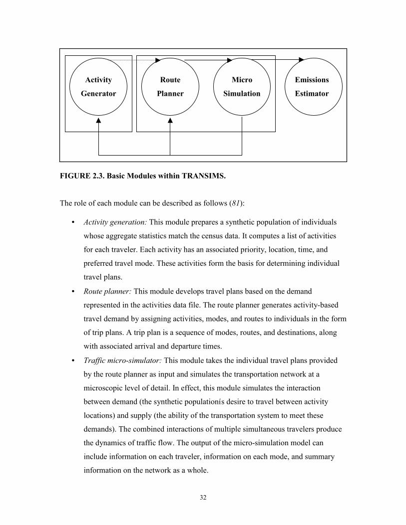
  32

 FIGURE 2.3. Basic Modules within TRANSIMS.   The role of each module can be described as follows (81):  

• Activity generation: This module prepares a synthetic population of individuals 

whose aggregate statistics match the census data. It computes a list of activities 

for each traveler. Each activity has an associated priority, location, time, and 

preferred travel mode. These activities form the basis for determining individual 

travel plans. 

• Route planner: This module develops travel plans based on the demand 

represented in the activities data file. The route planner generates activity-based 

travel demand by assigning activities, modes, and routes to individuals in the form 

of trip plans. A trip plan is a sequence of modes, routes, and destinations, along 

with associated arrival and departure times. 

• Traffic micro-simulator: This module takes the individual travel plans provided 

by the route planner as input and simulates the transportation network at a 

microscopic level of detail. In effect, this module simulates the interaction 

between demand (the synthetic populationís desire to travel between activity 

locations) and supply (the ability of the transportation system to meet these 

demands). The combined interactions of multiple simultaneous travelers produce 

the dynamics of traffic flow. The output of the micro-simulation model can 

include information on each traveler, information on each mode, and summary 

information on the network as a whole. 

Activity 

Generator 

Route 

Planner 

Micro 

Simulation 

Emissions 

Estimator 

  33

• Emissions estimator: This module translates traveler behavior into estimates of air 

quality, energy consumption, and carbon dioxide emissions. It should be noted, 

however, that while the vehicles are modeled at a microscopic level of detail their 

emissions are not estimated within the micro-simulation module; they are instead 

estimated in a separate module from more aggregate output data. This approach 

was adopted because there is no guarantee that the microscopic speed profiles 

produced by the TRANSIMS micro-simulator are accurate or even reasonable. 

 

  Note that TRANSIMS relies heavily on feedback in that congestion, as measured in 

the micro-simulation, can affect the synthetic populationís activities, plans, and routes. 

Details of the full model may be found elsewhere (79,80,81). 

  A key concept in the TRANSIMS micro-simulator logic is the particle hopping and 

cellular automata models. Particle hopping models originated from work by physicists to 

describe particle movement. Cellular automata is a subset of particle hopping models and 

is conceptually quite simple. It is this simplicity that allows it to be used to simulate 

traffic networks down to the driveway level, in a reasonable amount of time and 

accuracy. Cellular automata operates on an array of small clearly bounded locations or 

cells that are 7.5 m in length. Each cell can be either occupied by a vehicle or empty. The 

vehicles are moved through the network by a set of rules, which controls aspects such as 

acceleration, deceleration, and lane changing. The velocity of a given vehicle is an 

integer number that ranges from zero to five cells per second, which translates to a range 

from 0 to 135 km/h in steps of 27 km/h (79). 

 

Environmental Models 

Air Pollution Models 

  The most commonly used vehicular emission model in North America is the 

MOBILE 5a model. This model estimates volatile organic compounds (VOCs), carbon 

monoxide (CO), and nitrogen oxide (NOx) emissions from highway vehicles. The 

emission rates produced by the model are developed on a disaggregate level and an 

attempt is made to consider aspects such as the operating mode (cold start, hot start, and 

  34

stabilized conditions) (82). The application of the emission rates to obtain total air 

pollution values, however, is mostly done on an aggregate level. 

  There are numerous other initiatives to develop and refine vehicle emission models. 

These initiatives are attempting to increase prediction accuracy by using more extensive 

databases and to conduct the modeling on a more microscopic level. Some of these 

initiatives in the United States are as follows (83): 

 

• The EPA model being developed by the Georgia Institute of Technology; 

• The National Cooperative Highway Research Program (NCHRP) Modal Model 

being developed by the University of California at Riverside; 

• Modal emission projects completed by the University of Michigan;  

• Various models developed by the California Air Resources Board (CARB); 

• The EMFAC model developed by the California Department of Transportation; 

and 

• The MOBILE 6 model currently being developed by the Office of Mobile Studies 

of the EPA. 

 

Noise Pollution Models 

  Most traffic noise models estimate noise as a line source rather than per individual 

vehicle. The noise impact is estimated based on a variety of variables associated with the 

traffic stream and the surrounding environment. Factors that influence noise levels can be 

divided into those that influence noise generation and those that affect noise propagation. 

Factors influencing noise generation from vehicles include average flow rate, 

composition of the vehicle stream, average speed, road surface and tire interface, 

roadway gradient, and proximity of the site to a junction. The propagation of noise 

between the source and the receiver is dependent upon several factors including the 

distance between the source and the receiver, the amount and type of ground cover, the 

presence of sound barriers, the angle of view of the receiver, reflection by facades, and 

the road width (84). 

  There are a number of vehicle noise models developed across the world, and the 

following are some of the more widely known ones (84,85): 

  35

• The U.K. DoE model developed in the United Kingdom; 

• Various versions of the STAMINA model developed in the United States; 

• The Transport and Road Research Laboratory (TRRL) model developed in the 

United Kingdom; and 

• The new Federal Highway Administration Traffic Noise Prediction Model 

(FHWA TNM), which is currently under development by the Federal Highway 

Administration. This model is calibrated on a disaggregate data set comprising of 

6,000 individual pass-by events and will shortly become the state of the practice 

in traffic noise modeling in the United States. 

 

Fuel Consumption Models 

  Vehicular fuel consumption models are based on variables such as speed, 

acceleration, deceleration, fraction of time that the vehicle is stopped, and grade. These 

models are mostly calibrated based upon the characteristics of individual vehicles. There 

are a number of fuel consumption models available. The following are some of the better 

known models (77,86): 

 

• A model contained in the macroscopic simulation model, FREFLO;  

• ARFCOM, a detailed incremental power model developed by the Australian Road 

Research Board; 

• A model developed by Bester based on speed, acceleration, and gradient; 

• A module contained in the TRANSIT-7F signal coordination program; 

• NETSIM, which utilizes a table to determine the fuel consumption as a function 

of both acceleration and speed (this table is now also incorporated in the 

CORSIM traffic simulation model); and 

• Several other models that are only a function of speed such as FREQ10 and 

NETFLO. 

 

CONCLUDING REMARKS 

  While the term sustainable development is fairly recent, the modern principles 

associated with it date back to the eighteenth century when people became aware of the 

  36

human impact on the environment. Over the years the concept of sustainability has been 

much debated and argued over. A number of authors have provided definitions for 

sustainable development and sustainable transportation, although none of these 

definitions seem to capture all the essential aspects of sustainability. 

  Current legislation, planning regulations, and policies are becoming more geared 

toward the principles of sustainable transportation. The actual implementation of these 

principles up to now have, however, been very disappointing, and successes are few and 

far between. Inadequate transportation planning practice is mostly blamed for the poor 

implementation record of sustainable transportation. Specific deficiencies include a lack 

of understanding and appreciation for sustainable transportation, as well as a lack of 

quantified measures to monitor progress and to assist with decision-making. 

  The challenge, therefore, is to identify and quantify appropriate performance 

measures for sustainable transportation and to use them in the decision-making process. 

The following levels of performance measures were identified, namely data, information, 

performance measures, indices, objectives, and goals. The highest levels of aggregation 

are direct products of a strategic planning exercise, whereas the two lowest levels are the 

products from operational management and data collection. The new trend in 

performance measures is for them to become more outcome oriented versus the 

traditional efficiency focus. Even though there are numerous performance measures that 

can be used in the context of sustainable transportation, there are still challenges 

associated with adequately and accurately quantifying such measures. 

  Models for quantifying performance measures for sustainable transportation include 

transportation models, transportation environmental impact models, and economic 

models. The state of the practice for these models is to base their information on 

aggregate data sets. Significant shortcomings of this approach are the inaccuracies due to 

a loss in detail and the effect of aggregation bias. There are very few examples where 

aspects related to sustainable transportation are calculated at a disaggregate level. The 

latest state of the art in transportation modeling and data collection techniques, however, 

make it possible to quantify performance measures at a disaggregate level. New ITS 

technologies, for example, make it possible to calculate individual travel times, whereas 

  37

new transportation models, such as TRANSIMS, make it possible to trace simulated 

individual commuters on a second-by-second basis. 

  The following chapter provides a more comprehensive definition for sustainable 

transportation and proposes a framework for identifying, quantifying, and using 

performance measures for sustainable transportation in the decision-making process. 

 

 

 

 

39 

CHAPTER 3: A FRAMEWORK FOR ACHIEVING SUSTAINABLE 

TRANSPORTATION  

  As discussed in the preceding chapters, the primary reason that sustainable 

transportation concepts have not been implemented successfully is that the concepts are 

still unclear and have not been adequately quantified. Apart from the lack of clarity with 

regard to the interpretation of sustainable transportation, the current state of the practice 

in modeling techniques is also inadequate to quantify the sustainable transportation 

performance measures at the appropriate level of detail and accuracy. There is, therefore, 

a need to define sustainable transportation and to put it in context with the broader issue 

of sustainable development. There is also a need to show how performance measures for 

sustainable transportation can be identified and how they can be quantified with the latest 

state of the art in data collection and modeling techniques. 

 

DEFINING SUSTAINABLE TRANSPORTATION 

  Various definitions have been proposed for sustainable development and sustainable 

transportation. It should be noted that all these definitions are based on the one adopted 

by the Brundtlandt commission (4). None of the proposed definitions, however, seems to 

capture all the essential aspects of sustainability. The authors propose the following 

definition for sustainable development for this research: ì sustainable development is 

development that ensures intergenerational equity by simultaneously addressing the 

multi-dimensional components of economic development, environmental stewardship, 

and social equity. It is a dynamic process, which considers the changing needs of society 

both spatially and temporally. Sustainable development can be viewed as a continuum, 

representing various degrees of sustainability. It must, however, be achieved within 

resource, environmental, and ecological constraints.î  

  The following principles of sustainable development are included in the definition: 

 

• Intergenerational equity: A major goal of sustainable development is to ensure 

that current and future generations can enjoy an acceptable quality of life. There 

  40

should also be an equitable distribution of resources between communities and 

generations. 

• Multi-dimensional: The three dimensions of sustainable development are 

economic development, environmental stewardship, and social equity. These 

dimensions are interrelated and must be simultaneously addressed in order to 

meet the needs of current and future generations.  

• Dynamic: In considering intergenerational equity it is necessary to take 

cognizance of the fact that the needs of societies change both spatially and 

temporally. 

• Continuum: Sustainability is not represented by discrete indications of 

sustainability or unsustainability, but rather as a continuum, which represents 

various degrees of sustainability. 

 The following constraints with regard to sustainable development are included in the 

definition: 

 

• Resource constraints: Non-renewable resources should not be used without 

enabling the production of substitutes, and renewable resources should not be 

used at a faster rate than they can be reproduced. 

• Ecological constraints: The ecological boundaries are exceeded if more waste is 

dumped into the ecological system than the system can safely absorb, or if the 

system is damaged by taking excessive amounts of good, arable land to provide 

transportation infrastructure. 

• Environmental constraints: The environment is damaged by excessive pollution 

that can result in ill health for humans and animals, and damage to plant species. 

Pollution can also result in climate changes, which can cause floods, droughts, 

and increased diseases. 

 

  unstainability can be measured against the needs of communities. Each community 

and each sector within each community, however, have different needs and expectations 

regarding the principles of sustainable development. These needs are not consistent and 

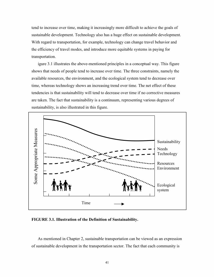
  41

tend to increase over time, making it increasingly more difficult to achieve the goals of 

sustainable development. Technology also has a huge effect on sustainable development. 

With regard to transportation, for example, technology can change travel behavior and 

the efficiency of travel modes, and introduce more equitable systems in paying for 

transportation. 

  igure 3.1 illustrates the above-mentioned principles in a conceptual way. This figure 

shows that needs of people tend to increase over time. The three constraints, namely the 

available resources, the environment, and the ecological system tend to decrease over 

time, whereas technology shows an increasing trend over time. The net effect of these 

tendencies is that sustainability will tend to decrease over time if no corrective measures 

are taken. The fact that sustainability is a continuum, representing various degrees of 

sustainability, is also illustrated in this figure. 

 

FIGURE 3.1. Illustration of the Definition of Sustainability.  

 

  As mentioned in Chapter 2, sustainable transportation can be viewed as an expression 

of sustainable development in the transportation sector. The fact that each community is 

  Sustainability 

Needs Technology  Resources Environment   

Ecological system 

Time 

Some Appropriate Measures 

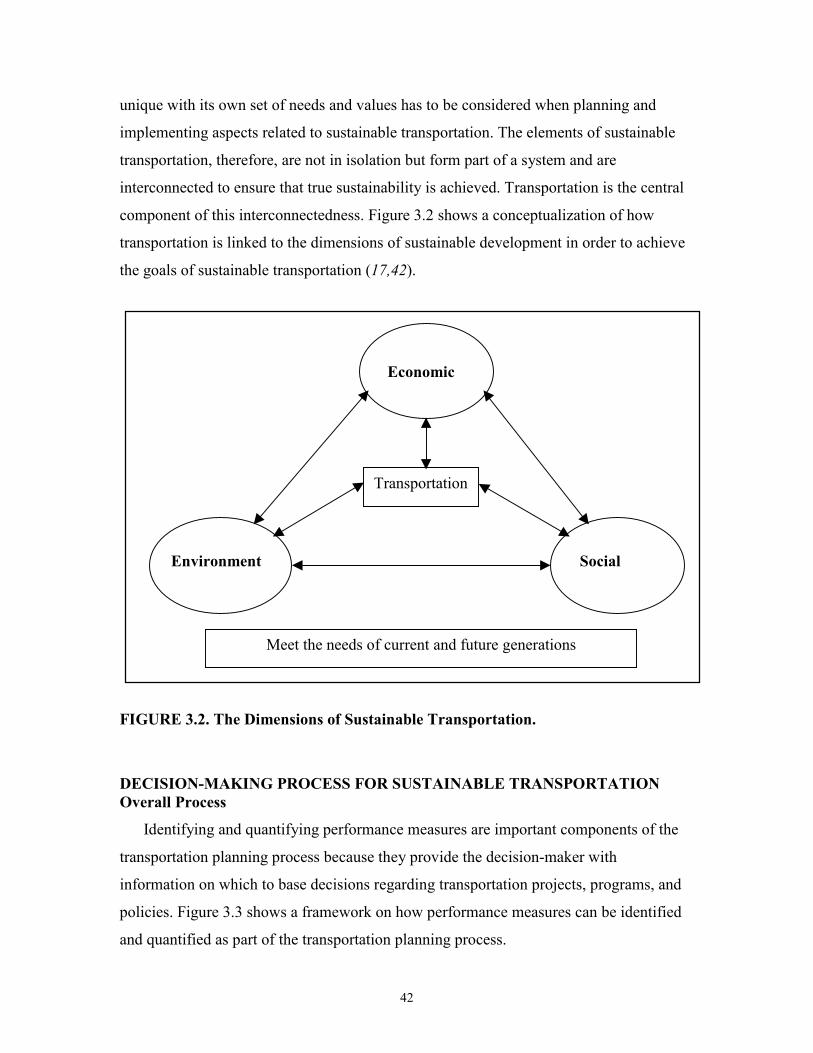
  42

unique with its own set of needs and values has to be considered when planning and 

implementing aspects related to sustainable transportation. The elements of sustainable 

transportation, therefore, are not in isolation but form part of a system and are 

interconnected to ensure that true sustainability is achieved. Transportation is the central 

component of this interconnectedness. Figure 3.2 shows a conceptualization of how 

transportation is linked to the dimensions of sustainable development in order to achieve 

the goals of sustainable transportation (17,42). 

 

FIGURE 3.2. The Dimensions of Sustainable Transportation.  

 DECISION-MAKING PROCESS FOR SUSTAINABLE TRANSPORTATION Overall Process 

  Identifying and quantifying performance measures are important components of the 

transportation planning process because they provide the decision-maker with 

information on which to base decisions regarding transportation projects, programs, and 

policies. Figure 3.3 shows a framework on how performance measures can be identified 

and quantified as part of the transportation planning process. 

 Economic  

Environment   Social 

Meet the needs of current and future generations 

Transportation

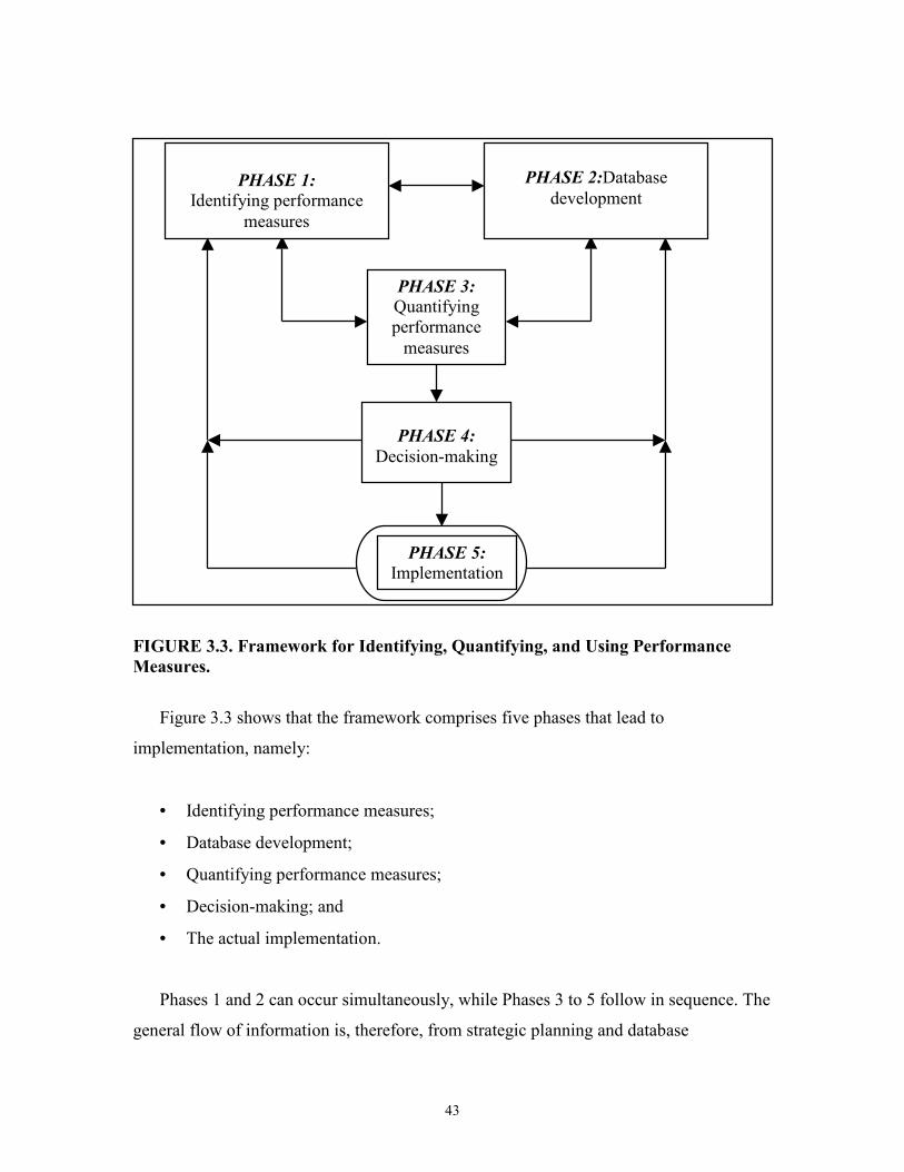
  43

 

 

FIGURE 3.3. Framework for Identifying, Quantifying, and Using Performance Measures.  

  Figure 3.3 shows that the framework comprises five phases that lead to 

implementation, namely: 

 

• Identifying performance measures; 

• Database development; 

• Quantifying performance measures; 

• Decision-making; and 

• The actual implementation. 

 

  Phases 1 and 2 can occur simultaneously, while Phases 3 to 5 follow in sequence. The 

general flow of information is, therefore, from strategic planning and database 

 PHASE 4: 

Decision-making 

PHASE 5: Implementation 

 PHASE 1: 

Identifying performance measures 

PHASE 2:Database development 

PHASE 3: Quantifying performance measures 

  44

development toward implementation. At the center of the activities is the quantification 

of performance measures, which is linked to Phases 1, 2, and 4. Once decision-making or 

implementation has occurred, feedback is required to the first two phases to ensure that 

any necessary adjustments can be made. Each of the five phases of the framework will 

now be discussed in turn to illustrate how they can be developed and applied. 

 

Phase 1: Identifying Performance Measures 

  The identification of appropriate performance measures is a very important task 

because poor performance measures can lead to poor decisions and poor outcomes. It 

should be noted that because interest groups such as the general public, engineers, 

managers, and decision-makers have different expectations, needs, and technical 

expertise, it is possible to identify different sets of performance measures. Engineers, for 

example, prefer a more quantitative approach and tend to strive for optimum results, 

whereas most decision-makers are very comfortable with a more qualitative approach. 

The increased demand for public participation requires performance measures that are 

understandable by the public at large. Consideration of the needs and technical abilities of 

the target group, therefore, is of key importance. The strategic planning approach is able 

to incorporate the needs and technical abilities of the various interest groups. 

  The strategic planning process is comprised of a number of steps. These steps are to 

develop a vision, mission, goals, objectives, strategies, policies, and actions. As discussed 

in Chapter 2, the process does not flow smoothly from one step to the next. It is at best a 

highly iterative process that requires consistent checks to ascertain whether the outcomes 

of the existing step of the process are consistent with what have been proposed in 

previous steps. 

  The strategic planning process is outlined in Figure 3.4, which shows that a Strengths, 

Weaknesses, Opportunities, and Threats (SWOT) analysis feeds into the determination of 

strategies and policies. The strengths and weaknesses refer to the internal strengths and 

weaknesses of the organization, whereas the opportunities and threats refer to external 

opportunities and threats that might impact upon the organization. The SWOT analysis is 

a powerful tool to ensure that the strategies and policies are both effective and realistic. 

  Figure 3.4 also shows that performance measures are identified at the levels of goals 

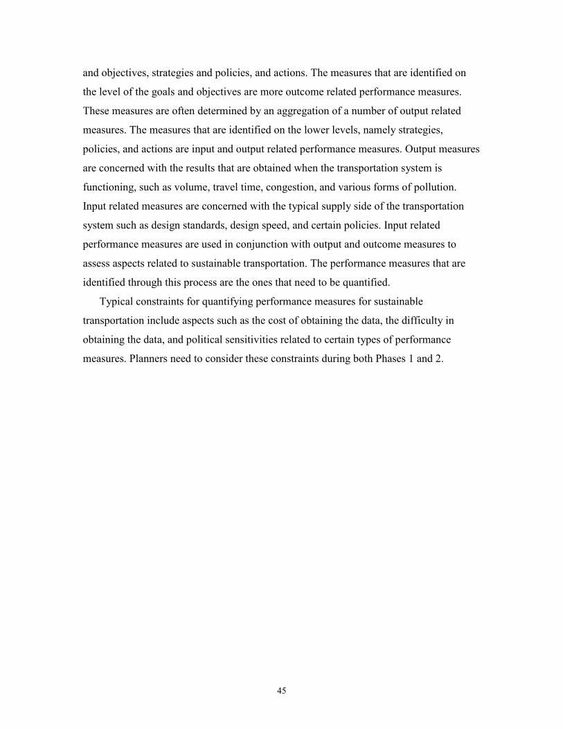
  45

and objectives, strategies and policies, and actions. The measures that are identified on 

the level of the goals and objectives are more outcome related performance measures. 

These measures are often determined by an aggregation of a number of output related 

measures. The measures that are identified on the lower levels, namely strategies, 

policies, and actions are input and output related performance measures. Output measures 

are concerned with the results that are obtained when the transportation system is 

functioning, such as volume, travel time, congestion, and various forms of pollution. 

Input related measures are concerned with the typical supply side of the transportation 

system such as design standards, design speed, and certain policies. Input related 

performance measures are used in conjunction with output and outcome measures to 

assess aspects related to sustainable transportation. The performance measures that are 

identified through this process are the ones that need to be quantified. 

  Typical constraints for quantifying performance measures for sustainable 

transportation include aspects such as the cost of obtaining the data, the difficulty in 

obtaining the data, and political sensitivities related to certain types of performance 

measures. Planners need to consider these constraints during both Phases 1 and 2. 

 

 

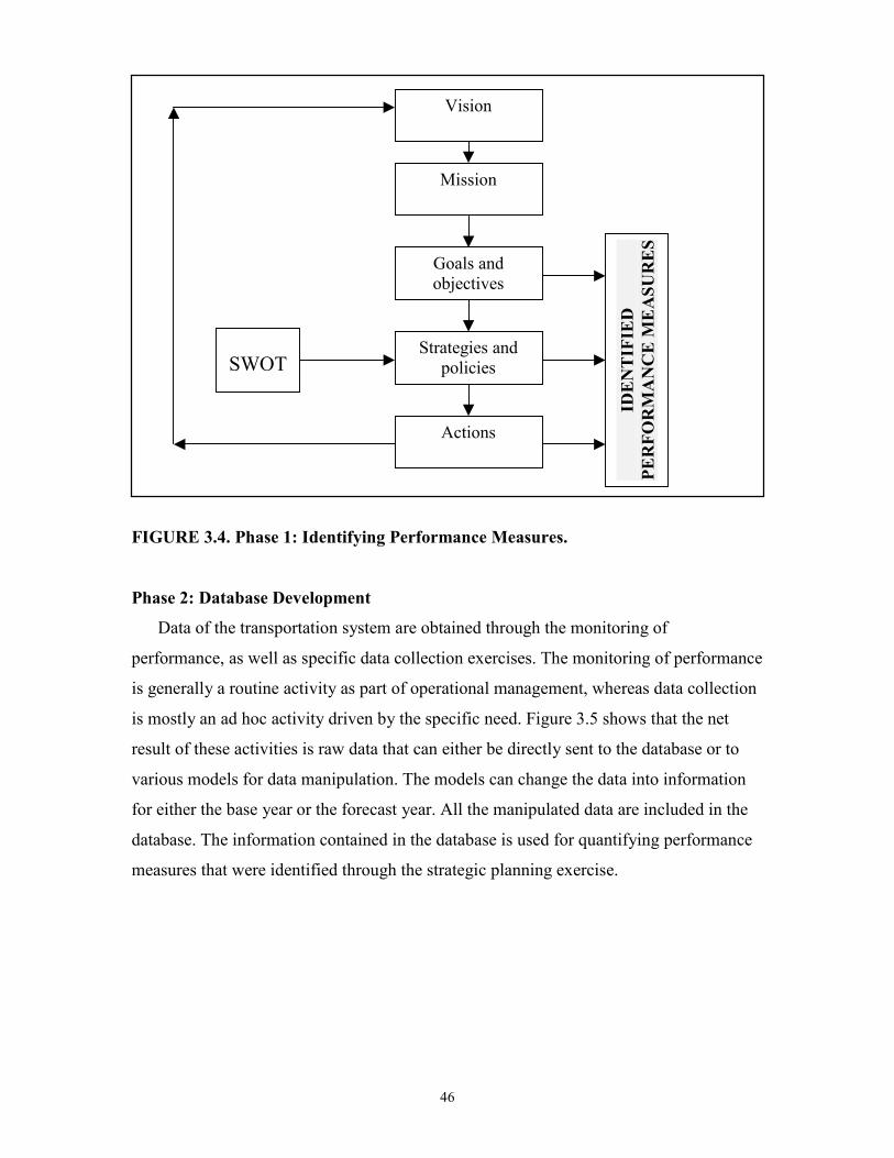
  46

 

FIGURE 3.4. Phase 1: Identifying Performance Measures.   Phase 2: Database Development 

  Data of the transportation system are obtained through the monitoring of 

performance, as well as specific data collection exercises. The monitoring of performance 

is generally a routine activity as part of operational management, whereas data collection 

is mostly an ad hoc activity driven by the specific need. Figure 3.5 shows that the net 

result of these activities is raw data that can either be directly sent to the database or to 

various models for data manipulation. The models can change the data into information 

for either the base year or the forecast year. All the manipulated data are included in the 

database. The information contained in the database is used for quantifying performance 

measures that were identified through the strategic planning exercise. 

Vision 

Mission 

Goals and objectives 

Strategies and policies 

Actions 

IDENTIFIED 

PERFORMANCE MEASURES 

SWOT 

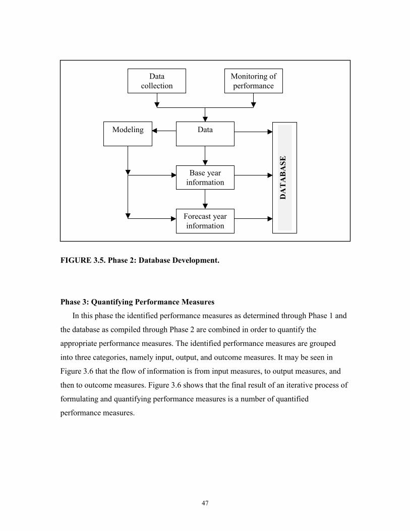
  47

 

FIGURE 3.5. Phase 2: Database Development. 

 

 

Phase 3: Quantifying Performance Measures 

  In this phase the identified performance measures as determined through Phase 1 and 

the database as compiled through Phase 2 are combined in order to quantify the 

appropriate performance measures. The identified performance measures are grouped 

into three categories, namely input, output, and outcome measures. It may be seen in 

Figure 3.6 that the flow of information is from input measures, to output measures, and 

then to outcome measures. Figure 3.6 shows that the final result of an iterative process of 

formulating and quantifying performance measures is a number of quantified 

performance measures. 

Data collection 

Monitoring of performance

Data 

Base year information 

Forecast year information 

Modeling 

DATABASE

 

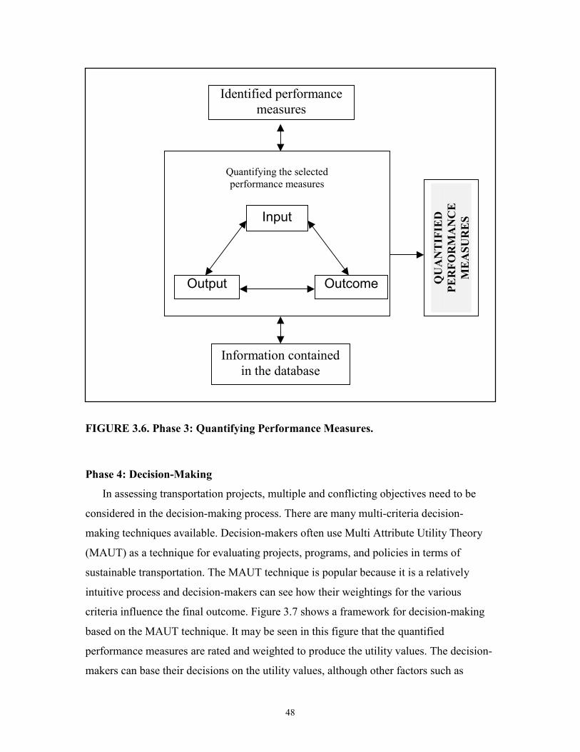
  48

 

FIGURE 3.6. Phase 3: Quantifying Performance Measures. 

  Phase 4: Decision-Making 

  In assessing transportation projects, multiple and conflicting objectives need to be 

considered in the decision-making process. There are many multi-criteria decision-

making techniques available. Decision-makers often use Multi Attribute Utility Theory 

(MAUT) as a technique for evaluating projects, programs, and policies in terms of 

sustainable transportation. The MAUT technique is popular because it is a relatively 

intuitive process and decision-makers can see how their weightings for the various 

criteria influence the final outcome. Figure 3.7 shows a framework for decision-making 

based on the MAUT technique. It may be seen in this figure that the quantified 

performance measures are rated and weighted to produce the utility values. The decision- 

makers can base their decisions on the utility values, although other factors such as 

Information contained in the database 

Input 

OutcomeOutput  QUANTIFIED 

PERFORMANCE 

MEASURES 

Identified performance measures 

Quantifying the selected performance measures 

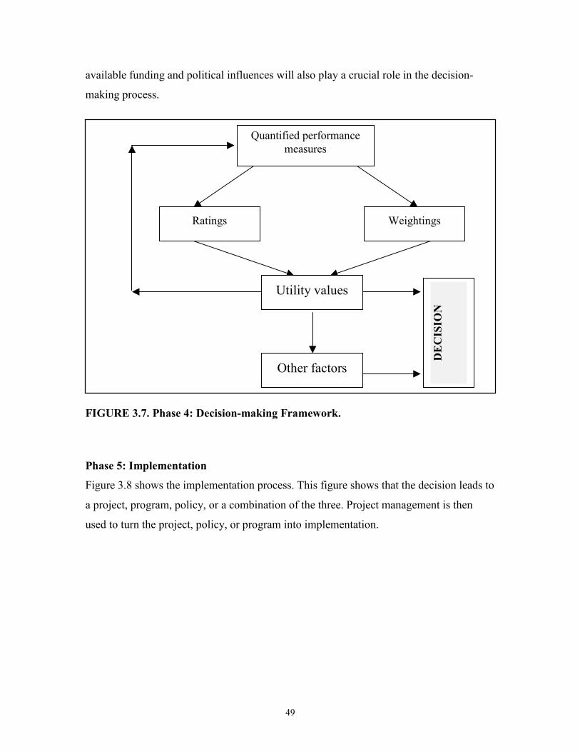
  49

available funding and political influences will also play a crucial role in the decision-

making process. 

 FIGURE 3.7. Phase 4: Decision-making Framework.  

 

Phase 5: Implementation 

Figure 3.8 shows the implementation process. This figure shows that the decision leads to 

a project, program, policy, or a combination of the three. Project management is then 

used to turn the project, policy, or program into implementation. 

Quantified performance measures 

Ratings  Weightings 

DECISION 

Utility values 

Other factors 

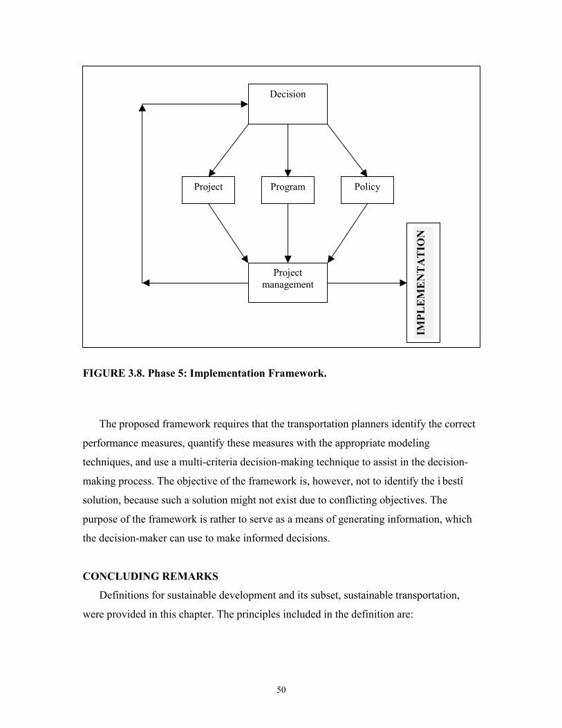
  50

 

FIGURE 3.8. Phase 5: Implementation Framework.  

 

  The proposed framework requires that the transportation planners identify the correct 

performance measures, quantify these measures with the appropriate modeling 

techniques, and use a multi-criteria decision-making technique to assist in the decision-

making process. The objective of the framework is, however, not to identify the ì bestî  

solution, because such a solution might not exist due to conflicting objectives. The 

purpose of the framework is rather to serve as a means of generating information, which 

the decision-maker can use to make informed decisions. 

 

CONCLUDING REMARKS 

  Definitions for sustainable development and its subset, sustainable transportation, 

were provided in this chapter. The principles included in the definition are: 

Decision 

Program

Project management 

IMPLEMENTATION 

Policy Project 

  51

 i) intergenerational equity; ii) multi-dimensional; iii) dynamic over space and time; and 

iv) continuum. Constraints that may directly influence sustainability are i) resource 

constraints; ii) ecological constraints; and iii) environmental constraints. 

  The authors proposed a framework on how to identify, quantify, and use performance 

measures for sustainable transportation in the transportation planning process. The 

framework comprises the following five phases that are interlinked to ensure adequate 

feedback and information flow: 

 

• Identifying performance measures; 

• Database development; 

• Quantifying performance measures; 

• Decision-making; and 

• Implementation. 

 

  A comprehensive investigation into important mobility and reliability related 

performance measures, namely travel time and travel time variability, is provided. A test 

bed comprising of two freeway corridors is introduced that forms the basis for the various 

applications. Observed AVI data is used to quantify travel time and travel time variability 

at various levels of aggregation, as well as at the level of the individual commuter.  

The following chapters will illustrate how this framework can be applied to identify and 

quantify performance measures for sustainable transportation. 

 

 

 

 

 

53 

CHAPTER 4: TRAVEL TIME ANALYSIS FROM ITS DATA  

  In Chapter 3 the authors propose a framework on identifying, quantifying, and using 

performance measures for sustainable transportation in the transportation planning 

process. This chapter focuses on Phases 1, 2, and 3, namely identification of performance 

measures, database development, and quantifying performance measures. The level of the 

individual commuter is an important component of disaggregate analysis. In this chapter, 

observed AVI data is used for quantifying travel time and travel time variability at the 

level of the individual commuter, as well as a number of levels of aggregation. 

 

DESCRIPTION OF THE TEST BED 

  A 22 km section of the Interstate 10 (I-10) corridor and a 21 km section of the US-

290 corridor in Houston, Texas, were selected as test beds for this research. Figure 4.1 

shows a location map of the freeway system in the Houston area. The locations of the two 

test corridors relative to the other major freeways, as well as the locations the AVI 

stations, are shown in this figure. Both test corridors are divided freeways with full grade 

separation, three to four lanes per direction, and high occupancy vehicle (HOV) facilities 

in the median. 

  The portion of the I-10 corridor stretches from just west of the Barker Cypress entry 

to just east of the Silber entry, which is approximately seven kilometers from the central 

business district (CBD) of Houston. This section of freeway comprises fourteen on-

ramps, twelve off-ramps, and five AVI stations. Each merge and diverge point, as well as 

the AVI stations, were considered as nodes, which resulted in a total of twenty-eight links 

associated with on- and off-ramps (freeway links) and four larger links associated with 

AVI stations (AVI links). The portion of the US-290 corridor stretches from just east of 

the FM 1960 entry to just west of the I-610 exit, which is approximately eight kilometers 

from the CBD of Houston. This section of freeway is comprised of eleven on-ramps, 

twelve off-ramps, and six AVI stations, which resulted in twenty-four freeway links and 

five AVI links. 

 

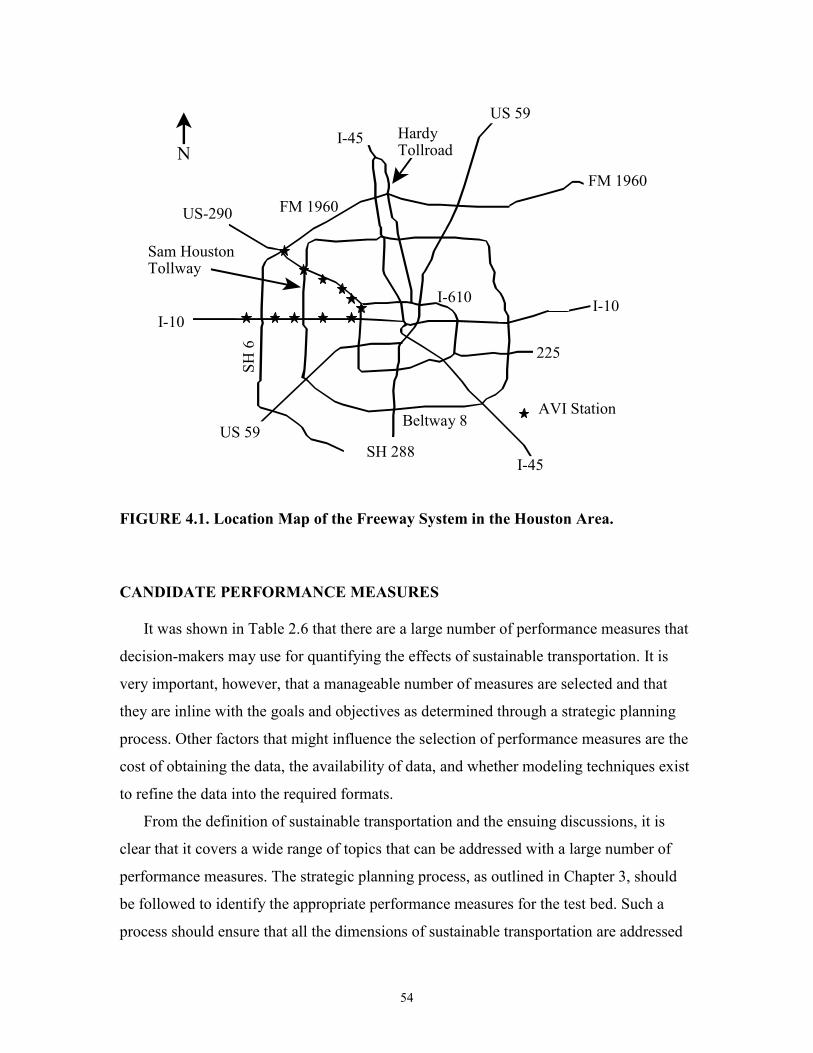
  54

US-290

I-45

I-610I-10

US 59

US 59

I-45 HardyTollroad

AVI Station

N

Sam HoustonTollway

FM 1960

225

I-10

FM 1960

SH 6

Beltway 8

SH 288 

 

FIGURE 4.1. Location Map of the Freeway System in the Houston Area.  

 

CANDIDATE PERFORMANCE MEASURES    It was shown in Table 2.6 that there are a large number of performance measures that 

decision-makers may use for quantifying the effects of sustainable transportation. It is 

very important, however, that a manageable number of measures are selected and that 

they are inline with the goals and objectives as determined through a strategic planning 

process. Other factors that might influence the selection of performance measures are the 

cost of obtaining the data, the availability of data, and whether modeling techniques exist 

to refine the data into the required formats. 

  From the definition of sustainable transportation and the ensuing discussions, it is 

clear that it covers a wide range of topics that can be addressed with a large number of 

performance measures. The strategic planning process, as outlined in Chapter 3, should 

be followed to identify the appropriate performance measures for the test bed. Such a 

process should ensure that all the dimensions of sustainable transportation are addressed 

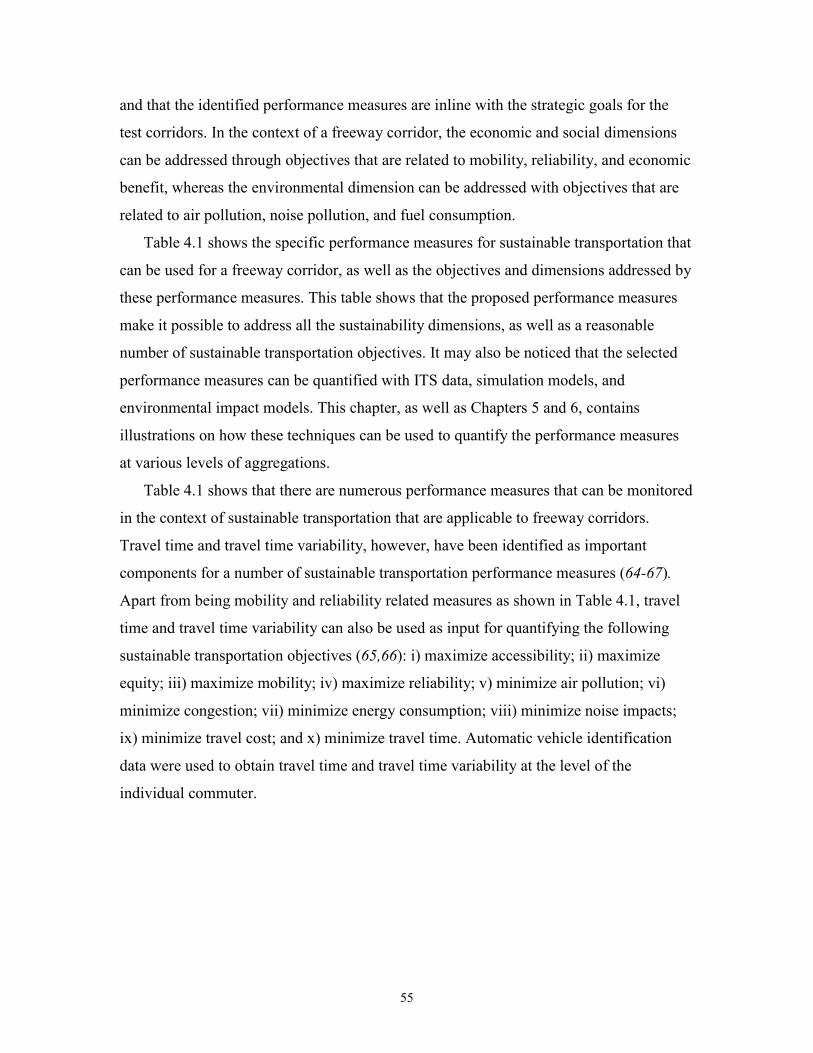
  55

and that the identified performance measures are inline with the strategic goals for the 

test corridors. In the context of a freeway corridor, the economic and social dimensions 

can be addressed through objectives that are related to mobility, reliability, and economic 

benefit, whereas the environmental dimension can be addressed with objectives that are 

related to air pollution, noise pollution, and fuel consumption. 

  Table 4.1 shows the specific performance measures for sustainable transportation that 

can be used for a freeway corridor, as well as the objectives and dimensions addressed by 

these performance measures. This table shows that the proposed performance measures 

make it possible to address all the sustainability dimensions, as well as a reasonable 

number of sustainable transportation objectives. It may also be noticed that the selected 

performance measures can be quantified with ITS data, simulation models, and 

environmental impact models. This chapter, as well as Chapters 5 and 6, contains 

illustrations on how these techniques can be used to quantify the performance measures 

at various levels of aggregations. 

  Table 4.1 shows that there are numerous performance measures that can be monitored 

in the context of sustainable transportation that are applicable to freeway corridors. 

Travel time and travel time variability, however, have been identified as important 

components for a number of sustainable transportation performance measures (64-67). 

Apart from being mobility and reliability related measures as shown in Table 4.1, travel 

time and travel time variability can also be used as input for quantifying the following 

sustainable transportation objectives (65,66): i) maximize accessibility; ii) maximize 

equity; iii) maximize mobility; iv) maximize reliability; v) minimize air pollution; vi) 

minimize congestion; vii) minimize energy consumption; viii) minimize noise impacts; 

ix) minimize travel cost; and x) minimize travel time. Automatic vehicle identification 

data were used to obtain travel time and travel time variability at the level of the 

individual commuter. 

 

  56

TABLE 4.1  Performance Measures for a Transportation Corridor 

 Analysis Technique  

Sustainability Dimension 

Objective  Performance Measures 

AVI data and traffic simulation models 

Economic, social     Economic, social    Economic  

Maximize reliability     Maximize mobility     Maximize economic benefit  

Standard deviation of travel time, or coefficient of variation of travel time  Total delay, travel rate, travel time, % corridor congested, and LOS  Net present worth 

Traffic simulation models, emission models, noise models, and fuel consumption models 

Environmental   Environmental   Environmental 

Minimize air pollution   Minimize noise impacts  Minimize energy use 

VOC, CO, and NOx emissions  Noise levels   Fuel consumption 

  

DESCRIPTION OF THE AVI DATA 

  The AVI system in Houston comprises AVI reader stations, a large pool of vehicles 

that have AVI tags fitted to them (probe vehicles), and a central computer system. The 

probe vehicles are comprised of vehicles whose owners use the electronic capabilities of 

the Houston tollway network or who have voluntarily placed AVI tags in their vehicles. 

The AVI stations are spaced at intervals that range from one to ten miles, and there may 

be highway interchanges located between them. When the data was collected in 1996, 

there were 113 AVI stations located throughout the Houston freeway network, resulting 

in approximately 340,000 reads per day. The first stage of adding AVI readers on the 

arterial system is currently underway, which means that AVI data can be used in the 

future to determine performance measures for sustainable transportation on arterial 

roadways, as well as freeways. 

  57

  When a probe vehicle passes a roadside reader unit, the information on the 

transponder is read by the reader unit and transferred to the central computer. The 

information that is sent to the central computer will include the vehicleís identification 

number, the time that it was read, the date that it was read, and the number of the reader 

unit that performed the read. For computing travel times, the central computer monitors 

several consecutive reader units and matches the transponder identification numbers. In 

the data provided for this research, the identification numbers were randomized to yield 

anonymous identification numbers so that the privacy of the commuters could be 

protected. 

  For the purpose of this research, the AVI data for sixty-two consecutive weekdays 

during September, October, and November of 1996 were obtained. The morning peak 

period, which was identified as lasting from 6 a.m. to 9 a.m., was selected as the analysis 

period. The three-hour period was divided into twelve fifteen-minute time increments to 

ensure that a reasonable number of observations (an average of 120 per time increment) 

were obtained for each of the corridors. It should also be noted that in the Highway 

Capacity Manual (HCM) the fundamental flow parameters are usually based on point 

observations over a fifteen-minute period (87). 

  Factors such as congestion, driver behavior, incidents, and weather condition can all 

influence the travel time and travel time distribution. No major incidents were noticed 

during the analysis period and no attempt was made to exclude any observations as a 

result of any of the above-mentioned factors. In analyzing AVI data at the disaggregate 

level, it was assumed that the same driver used the specific vehicle every time that it was 

detected on the corridor. This assumption can be regarded as reasonable because for 

commuter trips the same driver normally drives the same vehicle. 

  When a very long travel time was observed, it was necessary to determine whether 

such a travel time was due to congested conditions or because the vehicle had left the 

freeway to make a stop before re-entering upstream of the next AVI station. For this 

purpose, primary and secondary threshold values were used as proposed by Dixon (88). 

The threshold values used for this purpose were based on rolling means, standard 

deviations, and medians that are based on the previous ten observations. The primary 

threshold value was calculated by: i) assuming that the travel times were normally 

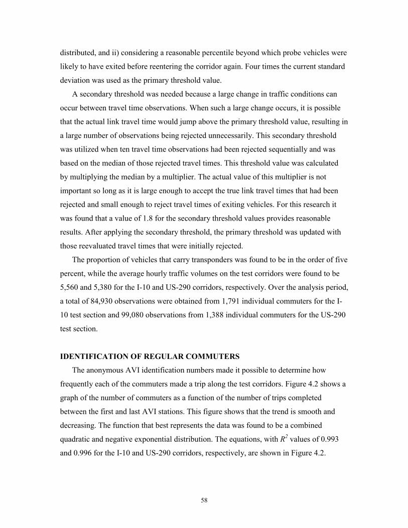
  58

distributed, and ii) considering a reasonable percentile beyond which probe vehicles were 

likely to have exited before reentering the corridor again. Four times the current standard 

deviation was used as the primary threshold value. 

  A secondary threshold was needed because a large change in traffic conditions can 

occur between travel time observations. When such a large change occurs, it is possible 

that the actual link travel time would jump above the primary threshold value, resulting in 

a large number of observations being rejected unnecessarily. This secondary threshold 

was utilized when ten travel time observations had been rejected sequentially and was 

based on the median of those rejected travel times. This threshold value was calculated 

by multiplying the median by a multiplier. The actual value of this multiplier is not 

important so long as it is large enough to accept the true link travel times that had been 

rejected and small enough to reject travel times of exiting vehicles. For this research it 

was found that a value of 1.8 for the secondary threshold values provides reasonable 

results. After applying the secondary threshold, the primary threshold was updated with 

those reevaluated travel times that were initially rejected. 

  The proportion of vehicles that carry transponders was found to be in the order of five 

percent, while the average hourly traffic volumes on the test corridors were found to be 

5,560 and 5,380 for the I-10 and US-290 corridors, respectively. Over the analysis period, 

a total of 84,930 observations were obtained from 1,791 individual commuters for the I-

10 test section and 99,080 observations from 1,388 individual commuters for the US-290 

test section. 

 

IDENTIFICATION OF REGULAR COMMUTERS 

  The anonymous AVI identification numbers made it possible to determine how 

frequently each of the commuters made a trip along the test corridors. Figure 4.2 shows a 

graph of the number of commuters as a function of the number of trips completed 

between the first and last AVI stations. This figure shows that the trend is smooth and 

decreasing. The function that best represents the data was found to be a combined 

quadratic and negative exponential distribution. The equations, with R2 values of 0.993 

and 0.996 for the I-10 and US-290 corridors, respectively, are shown in Figure 4.2. 

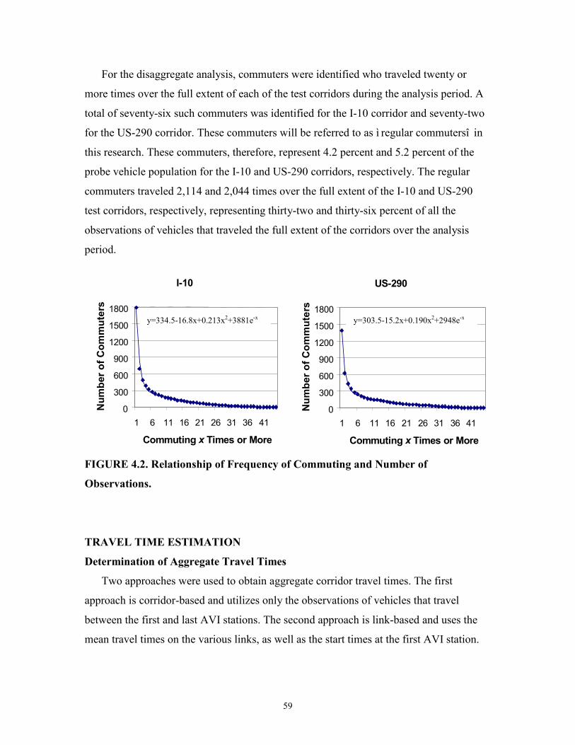
  59

For the disaggregate analysis, commuters were identified who traveled twenty or 

more times over the full extent of each of the test corridors during the analysis period. A 

total of seventy-six such commuters was identified for the I-10 corridor and seventy-two 

for the US-290 corridor. These commuters will be referred to as ì regular commutersî  in 

this research. These commuters, therefore, represent 4.2 percent and 5.2 percent of the 

probe vehicle population for the I-10 and US-290 corridors, respectively. The regular 

commuters traveled 2,114 and 2,044 times over the full extent of the I-10 and US-290 

test corridors, respectively, representing thirty-two and thirty-six percent of all the 

observations of vehicles that traveled the full extent of the corridors over the analysis 

period. 

FIGURE 4.2. Relationship of Frequency of Commuting and Number of 

Observations. 

 

 

TRAVEL TIME ESTIMATION 

Determination of Aggregate Travel Times 

  Two approaches were used to obtain aggregate corridor travel times. The first 

approach is corridor-based and utilizes only the observations of vehicles that travel 

between the first and last AVI stations. The second approach is link-based and uses the 

mean travel times on the various links, as well as the start times at the first AVI station. 

I-10

0

300

600

900

1200

1500

1800

1 6 11 16 21 26 31 36 41

Commuting x Times or More

Number of Com

muters

US-290

0

300

600

900

1200

1500

1800

1 6 11 16 21 26 31 36 41

Commuting x Times or More

Num

ber of Com

muters

y=334.5-16.8x+0.213x2+3881e-x  y=303.5-15.2x+0.190x2+2948e-x 

  60

  In terms of the corridor-based approach, the mean corridor travel time can be 

computed as a function of time of day and for each day analyzed, as shown in Equation 

4.1. This technique of aggregation will be referred to as the aggregation by day (ABD) 

approach, because it is based on aggregate data for each day and corridor-entering time 

interval. A further form of aggregation was obtained by combining the data from all the 

days while still keeping the corridor-entering time intervals separate as illustrated with 

Equation 4.2. This technique of aggregation will be referred to as the aggregation across 

days (AAD) approach, because it is based on aggregate data over a number of days. It is 

important to note that the latter approach has been adopted at a number of ITS 

deployment sites. 

 

cdtX  =  [ ]∑=

dtn

jcjdt

dt

Xn 1

1                 (4.1) 

 

ctX  =  [ ]∑∑= =

d dtn

d

n

jcjdt

t

Xn 1 1

1                (4.2) 

 

where: 

  cdtX   = Mean corridor travel time on day d and at time interval t 

  ctX    = Mean corridor travel time at time interval t and across all days 

  Xcjdt  = Corridor travel time for individual j on day d and time interval t 

  ndt  = Total number of observations on day d and at time interval t 

  nt  = Total number of observations in time interval t 

  nd  = Total number of days that were analyzed 

 

  The second approach for estimating corridor travel times uses link travel times 

because link travel times typically are the only information that is available. For ABD the 

mean travel time on each link was calculated as a function of time of day for each day 

analyzed. The corridor travel time was then estimated from the sample central moments 

as proposed by Fu and Rilett (89). This process involves the accumulation of link travel 

  61

times over the different time periods and for the different days. The time-dependent link 

travel time is modeled as a discrete step function. The arrival time at an AVI station falls 

into a specific time period, and the average link travel time of that period is then added to 

the current travel time in order to predict the arrival time at the next AVI station. This 

process is repeated for all the links along the corridor to yield the total corridor travel 

time. The recursive formula used to calculate mean corridor travel times for the ABD 

approach is shown as Equation 4.3. The mean corridor travel time for the AAD approach 

can also be determined with Equation 4.3, but mean travel times computed across days 

should be used instead of computed by days. 

 

( )∑=

−=jn

jjnj

jcdt TT

nX

11

1               (4.3) 

 

jT1 = Corridor-entering time of vehicle j; 

1112 dtjj XTT += ; 2223 dtjj XTT += Ö .,

1)1()1( −−− +=ndtnjnnj XTT  

 

where: 

  Xcdt        = Mean corridor travel time on day d and time interval t 

 11dtX       = Mean travel time on link 1 on day d and time interval  1t  

  njjj TTT ,..,, 21   = Arrival times at AVI stations 1, 2,Ö , n for vehicle j 

  nttt ,....,, 21    = Time intervals associated with arrival times  njjj TTT ,..,, 21  

 

  In order to obtain homogeneous samples, it was necessary to apply two constraints to 

the database. The first constraint states that only observations of vehicles that traversed 

the full extent of the corridors could be used, whereas the second constraint states that 

only trips that were observed at each of the AVI stations along the corridors could be 

used. Based on these constraints, sample sizes of 4,861 for I-10 and 3,943 for US-290 

were obtained over the analysis period. Both the corridor-based and the link-based 

approaches were used to determine the ABD and AAD travel time estimates for the two 

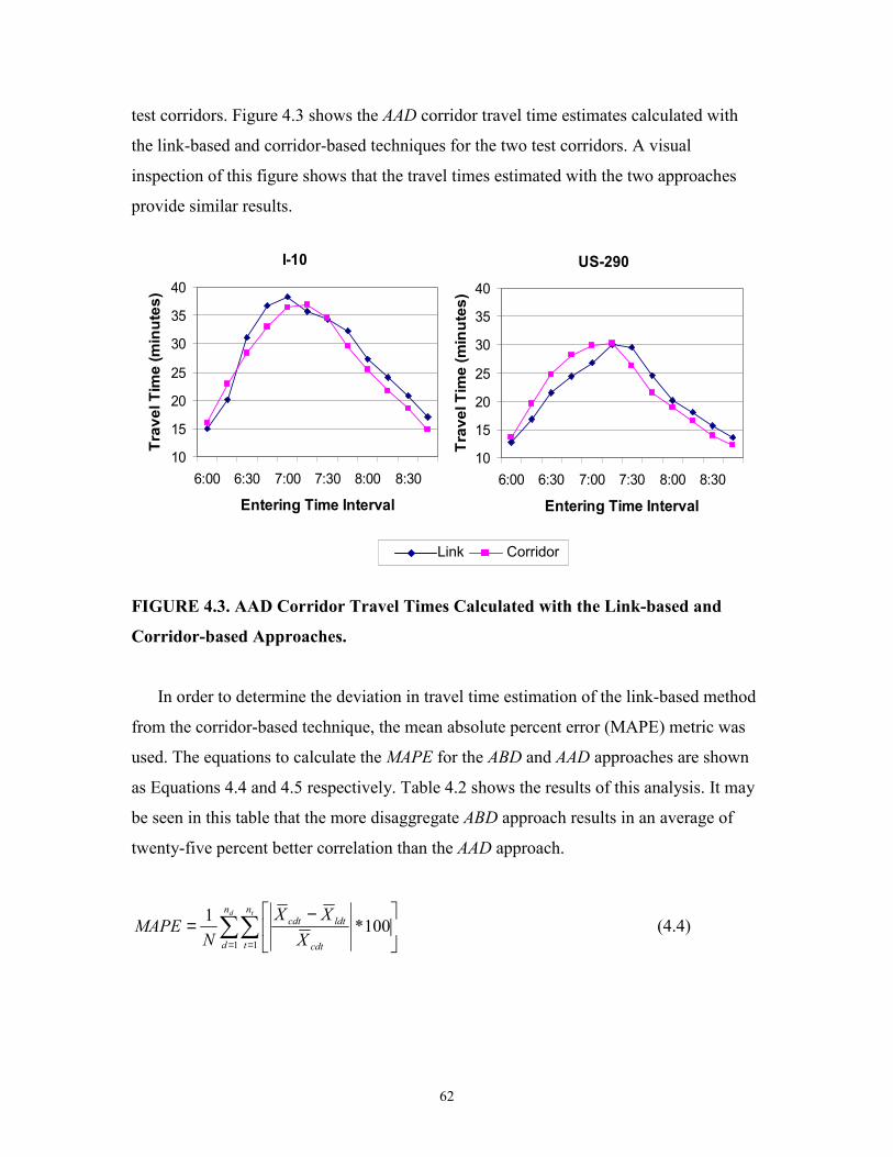
  62

test corridors. Figure 4.3 shows the AAD corridor travel time estimates calculated with 

the link-based and corridor-based techniques for the two test corridors. A visual 

inspection of this figure shows that the travel times estimated with the two approaches 

provide similar results. 

 

FIGURE 4.3. AAD Corridor Travel Times Calculated with the Link-based and 

Corridor-based Approaches. 

 

  In order to determine the deviation in travel time estimation of the link-based method 

from the corridor-based technique, the mean absolute percent error (MAPE) metric was 

used. The equations to calculate the MAPE for the ABD and AAD approaches are shown 

as Equations 4.4 and 4.5 respectively. Table 4.2 shows the results of this analysis. It may 

be seen in this table that the more disaggregate ABD approach results in an average of 

twenty-five percent better correlation than the AAD approach.  

 

∑∑= =

−=

d tn

d

n

t cdt

ldtcdt

XXX

NMAPE

1 1100*1           (4.4) 

 

I-10

10

15

20

25

30

35

40

6:00 6:30 7:00 7:30 8:00 8:30

Entering Time Interval

Travel Time (minutes)

US-290

10

15

20

25

30

35

40

6:00 6:30 7:00 7:30 8:00 8:30

Entering Time Interval

Travel Time (minutes)

Link  Corridor 

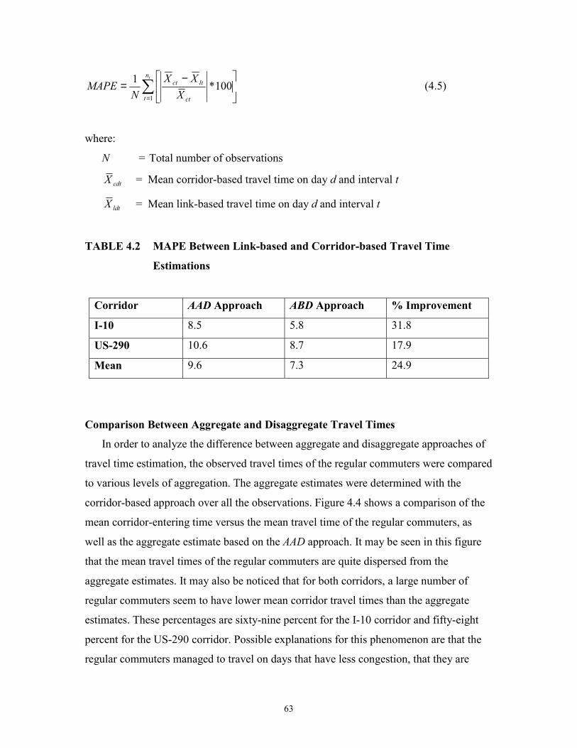
  63

∑=

−=

tn

t ct

ltct

XXX

NMAPE

1100*1             (4.5) 

 

where: 

  N     = Total number of observations 

  cdtX   =  Mean corridor-based travel time on day d and interval t   

  ldtX   =  Mean link-based travel time on day d and interval t   

 

TABLE 4.2  MAPE Between Link-based and Corridor-based Travel Time 

        Estimations 

 

Corridor  AAD Approach  ABD Approach  % Improvement 

I-10  8.5  5.8  31.8 

US-290  10.6  8.7  17.9 

Mean  9.6  7.3  24.9 

 

 

Comparison Between Aggregate and Disaggregate Travel Times 

  In order to analyze the difference between aggregate and disaggregate approaches of 

travel time estimation, the observed travel times of the regular commuters were compared 

to various levels of aggregation. The aggregate estimates were determined with the 

corridor-based approach over all the observations. Figure 4.4 shows a comparison of the 

mean corridor-entering time versus the mean travel time of the regular commuters, as 

well as the aggregate estimate based on the AAD approach. It may be seen in this figure 

that the mean travel times of the regular commuters are quite dispersed from the 

aggregate estimates. It may also be noticed that for both corridors, a large number of 

regular commuters seem to have lower mean corridor travel times than the aggregate 

estimates. These percentages are sixty-nine percent for the I-10 corridor and fifty-eight 

percent for the US-290 corridor. Possible explanations for this phenomenon are that the 

regular commuters managed to travel on days that have less congestion, that they are 

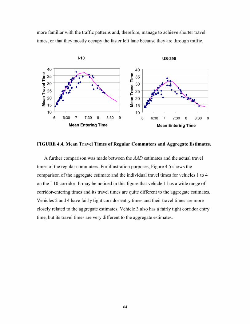
  64

more familiar with the traffic patterns and, therefore, manage to achieve shorter travel 

times, or that they mostly occupy the faster left lane because they are through traffic. 

 

FIGURE 4.4. Mean Travel Times of Regular Commuters and Aggregate Estimates.  

  A further comparison was made between the AAD estimates and the actual travel 

times of the regular commuters. For illustration purposes, Figure 4.5 shows the 

comparison of the aggregate estimate and the individual travel times for vehicles 1 to 4 

on the I-10 corridor. It may be noticed in this figure that vehicle 1 has a wide range of 

corridor-entering times and its travel times are quite different to the aggregate estimates. 

Vehicles 2 and 4 have fairly tight corridor entry times and their travel times are more 

closely related to the aggregate estimates. Vehicle 3 also has a fairly tight corridor entry 

time, but its travel times are very different to the aggregate estimates. 

I-10

10

15

20

25

30

35

40

6 6:30 7 7:30 8 8:30 9

Mean Entering Time

Mean Travel Time

US-290

10

15

20

25

30

35

40

6 6:30 7 7:30 8 8:30 9

Mean Entering TimeMean Travel Time

  65

 

FIGURE 4.5. Individual Travel Times and Aggregate Estimates Based on the AAD Approach.  

  In order to analyze the effect of a more disaggregate level of travel time estimation, 

the results from the ABD approach were compared to the actual travel times of the 

individual commuters traveling on the given days and within the time intervals. Figure 

4.6 shows the result obtained from this analysis for the same four vehicles as discussed 

above. It may be noticed that a much better prediction of the actual behavior is obtained 

when the travel time estimates are also disaggregated by individual days. This is 

particularly evident for vehicles 1 and 3 that show markedly better correlation with the 

ABD approach as compared to the AAD approach. 

 

Vehicle 1

10

20

30

40

50

6 6:30 7 7:30 8 8:30 9

Corridor Entering Time

Travel Time

Vehicle 2

10

20

30

40

50

6 6:30 7 7:30 8 8:30 9

Corridor Entering Time

Travel Time

Vehicle 3

10

20

30

40

50

6 6:30 7 7:30 8 8:30 9

Corridor Entering Time

Travel Time

Vehicle 4

10

20

30

40

50

6 6:30 7 7:30 8 8:30 9

Corridor Entering Time

Travel Time

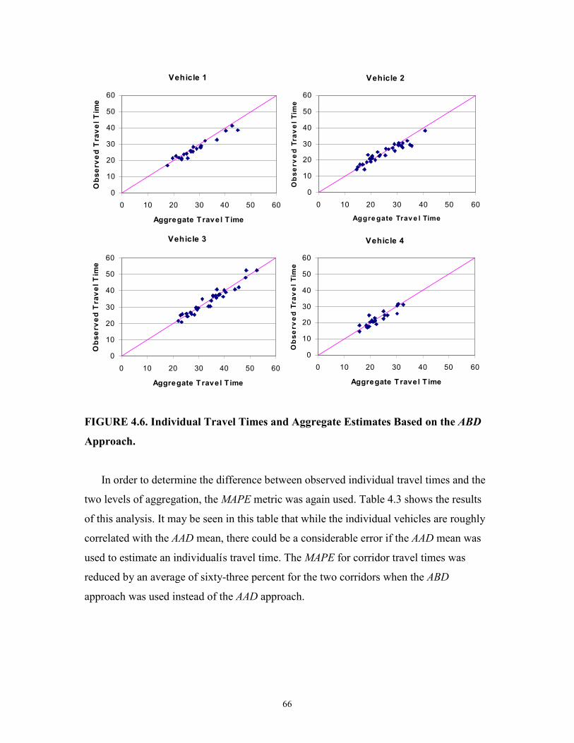
  66

 

FIGURE 4.6. Individual Travel Times and Aggregate Estimates Based on the ABD 

Approach. 

 

  In order to determine the difference between observed individual travel times and the 

two levels of aggregation, the MAPE metric was again used. Table 4.3 shows the results 

of this analysis. It may be seen in this table that while the individual vehicles are roughly 

correlated with the AAD mean, there could be a considerable error if the AAD mean was 

used to estimate an individualís travel time. The MAPE for corridor travel times was 

reduced by an average of sixty-three percent for the two corridors when the ABD 

approach was used instead of the AAD approach. 

 

 

Vehicle 1

0

10

20

30

40

50

60

0 10 20 30 40 50 60

Aggregate  Travel Time

Observed Travel Time

Vehicle 2

0

10

20

30

40

50

60

0 10 20 30 40 50 60

Aggregate  Trave l Time

Observed Travel Time

Vehicle 3

0

10

20

30

40

50

60

0 10 20 30 40 50 60

Aggregate  Travel Time

Observed Travel Time

Vehicle 4

0

10

20

30

40

50

60

0 10 20 30 40 50 60

Aggregate  Travel T ime

Observed

 Travel Time

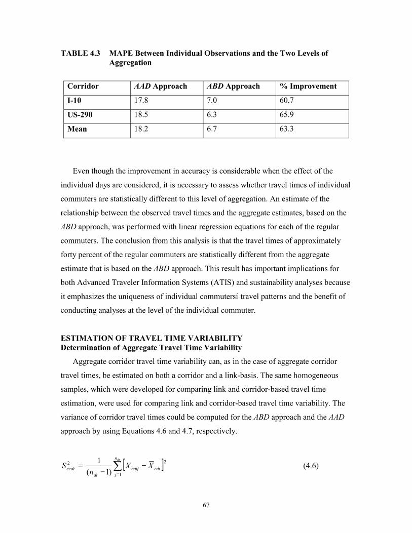
  67

TABLE 4.3  MAPE Between Individual Observations and the Two Levels of         Aggregation  

Corridor  AAD Approach  ABD Approach  % Improvement 

I-10  17.8  7.0  60.7 

US-290  18.5  6.3  65.9 

Mean  18.2  6.7  63.3 

 

 

  Even though the improvement in accuracy is considerable when the effect of the 

individual days are considered, it is necessary to assess whether travel times of individual 

commuters are statistically different to this level of aggregation. An estimate of the 

relationship between the observed travel times and the aggregate estimates, based on the 

ABD approach, was performed with linear regression equations for each of the regular 

commuters. The conclusion from this analysis is that the travel times of approximately 

forty percent of the regular commuters are statistically different from the aggregate 

estimate that is based on the ABD approach. This result has important implications for 

both Advanced Traveler Information Systems (ATIS) and sustainability analyses because 

it emphasizes the uniqueness of individual commutersí travel patterns and the benefit of 

conducting analyses at the level of the individual commuter. 

 

ESTIMATION OF TRAVEL TIME VARIABILITY Determination of Aggregate Travel Time Variability 

  Aggregate corridor travel time variability can, as in the case of aggregate corridor 

travel times, be estimated on both a corridor and a link-basis. The same homogeneous 

samples, which were developed for comparing link and corridor-based travel time 

estimation, were used for comparing link and corridor-based travel time variability. The 

variance of corridor travel times could be computed for the ABD approach and the AAD 

approach by using Equations 4.6 and 4.7, respectively. 

 

2ccdtS  =  [ ]∑

=

−−

dtn

jcdtcdtj

dt

XXn 1

2

)1(1             (4.6) 

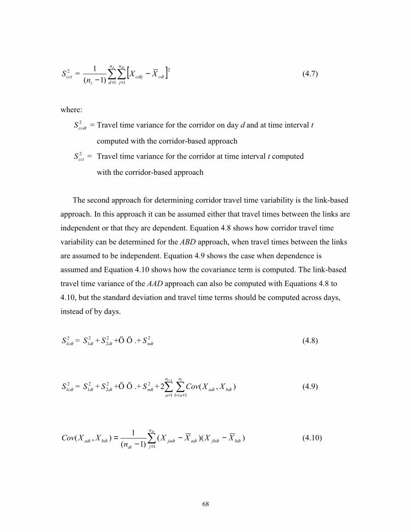
  68

 

2cctS  =  [ ]∑∑

= =

−−

d dtn

d

n

jcdtcdtj

t

XXn 1 1

2

)1(1             (4.7) 

 

where: 

  2ccdtS  = Travel time variance for the corridor on day d and at time interval t  

      computed with the corridor-based approach 

  2cctS  =  Travel time variance for the corridor at time interval t computed 

      with the corridor-based approach 

 

  The second approach for determining corridor travel time variability is the link-based 

approach. In this approach it can be assumed either that travel times between the links are 

independent or that they are dependent. Equation 4.8 shows how corridor travel time 

variability can be determined for the ABD approach, when travel times between the links 

are assumed to be independent. Equation 4.9 shows the case when dependence is 

assumed and Equation 4.10 shows how the covariance term is computed. The link-based 

travel time variance of the AAD approach can also be computed with Equations 4.8 to 

4.10, but the standard deviation and travel time terms should be computed across days, 

instead of by days. 

 2lcdtS =  2

1dtS + 22dtS +Ö Ö .+ 2

ndtS              (4.8) 

 

2lcdtS =  2

1dtS + 22dtS +Ö Ö .+ 2

ndtS + ∑ ∑−

= +=

1

1 1

),(2l ln

a

n

abbdtadt XXCov       (4.9) 

 

)()()1(

1),(1

bdtjbdt

n

jadtjadt

dtbdtadt XXXX

nXXCov

dt

−−−

= ∑=

      (4.10) 

 

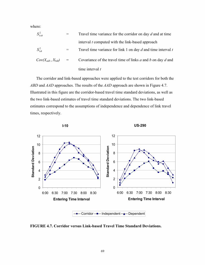
  69

where: 

  2lcdtS         =  Travel time variance for the corridor on day d and at time 

              interval t computed with the link-based approach 

  21dtS         =  Travel time variance for link 1 on day d and time interval t  

  Cov(Xadt , Xbdt)   =  Covariance of the travel time of links a and b on day d and 

              time interval t 

  The corridor and link-based approaches were applied to the test corridors for both the 

ABD and AAD approaches. The results of the AAD approach are shown in Figure 4.7. 

Illustrated in this figure are the corridor-based travel time standard deviations, as well as 

the two link-based estimates of travel time standard deviations. The two link-based 

estimates correspond to the assumptions of independence and dependence of link travel 

times, respectively. 

 

FIGURE 4.7. Corridor versus Link-based Travel Time Standard Deviations.  

I-10

0

2

4

6

8

10

12

6:00 6:30 7:00 7:30 8:00 8:30

Entering Time Interval

Standard Deviation

US-290

0

2

4

6

8

10

12

6:00 6:30 7:00 7:30 8:00 8:30

Entering Time Interval

Standard Deviation

Corridor Independent  Dependent 

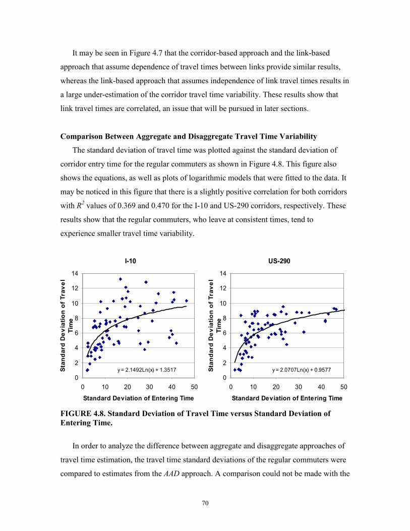
  70

  It may be seen in Figure 4.7 that the corridor-based approach and the link-based 

approach that assume dependence of travel times between links provide similar results, 

whereas the link-based approach that assumes independence of link travel times results in 

a large under-estimation of the corridor travel time variability. These results show that 

link travel times are correlated, an issue that will be pursued in later sections.  

 

Comparison Between Aggregate and Disaggregate Travel Time Variability 

  The standard deviation of travel time was plotted against the standard deviation of 

corridor entry time for the regular commuters as shown in Figure 4.8. This figure also 

shows the equations, as well as plots of logarithmic models that were fitted to the data. It 

may be noticed in this figure that there is a slightly positive correlation for both corridors 

with R2 values of 0.369 and 0.470 for the I-10 and US-290 corridors, respectively. These 

results show that the regular commuters, who leave at consistent times, tend to 

experience smaller travel time variability. 

FIGURE 4.8. Standard Deviation of Travel Time versus Standard Deviation of Entering Time.  

  In order to analyze the difference between aggregate and disaggregate approaches of 

travel time estimation, the travel time standard deviations of the regular commuters were 

compared to estimates from the AAD approach. A comparison could not be made with the 

I-10

y = 2.1492Ln(x) + 1.35170

2

4

6

8

10

12

14

0 10 20 30 40 50

Standard Deviation of Entering Time

Standard Deviation of Travel 

Time

US-290

y = 2.0707Ln(x) + 0.95770

2

4

6

8

10

12

14

0 10 20 30 40 50

Standard Deviation of Entering Time

Standard Deviation of Travel 

Time

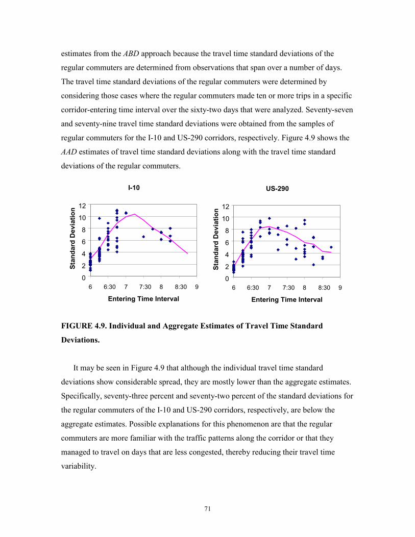
  71

estimates from the ABD approach because the travel time standard deviations of the 

regular commuters are determined from observations that span over a number of days. 

The travel time standard deviations of the regular commuters were determined by 

considering those cases where the regular commuters made ten or more trips in a specific 

corridor-entering time interval over the sixty-two days that were analyzed. Seventy-seven 

and seventy-nine travel time standard deviations were obtained from the samples of 

regular commuters for the I-10 and US-290 corridors, respectively. Figure 4.9 shows the 

AAD estimates of travel time standard deviations along with the travel time standard 

deviations of the regular commuters. 

 FIGURE 4.9. Individual and Aggregate Estimates of Travel Time Standard 

Deviations. 

 

  It may be seen in Figure 4.9 that although the individual travel time standard 

deviations show considerable spread, they are mostly lower than the aggregate estimates. 

Specifically, seventy-three percent and seventy-two percent of the standard deviations for 

the regular commuters of the I-10 and US-290 corridors, respectively, are below the 

aggregate estimates. Possible explanations for this phenomenon are that the regular 

commuters are more familiar with the traffic patterns along the corridor or that they 

managed to travel on days that are less congested, thereby reducing their travel time 

variability. 

I-10

0

2

4

6

8

10

12

6 6:30 7 7:30 8 8:30 9

Entering Time Interval

Standard Deviation

US-290

0

2

4

6

8

10

12

6 6:30 7 7:30 8 8:30 9

Entering Time Interval

Standard Deviation

  72

The MAPE metric was again used to compare the differences between the aggregate 

estimate of travel time variability that is based on the AAD approach and the observed 

travel time variability of the regular commuters. The MAPEs for the I-10 and US-290 

corridors were found to be very similar, namely 32.2 percent for the I-10 corridor and 

32.5 percent for the US-290 corridor. These results show that there is a considerable error 

associated with estimating travel time variability of individual commuters with the AAD 

approach. 

  The statistical differences between the travel time standard deviations of the regular 

commuters and the aggregate estimates based on the ABD approach were modeled as 

linear regression equations. The standard deviations of the regular commuters were again 

determined by considering those cases where they traveled the full extent of the corridor 

ten or more times during a particular corridor-entering time interval. For developing 

linear regression equations, only cases were considered that had three or more data 

points. The results from the tests indicated that the null hypothesis could be rejected for 

twenty percent of the days for the I-10 corridor and 15.4 percent of the days for the US-

290 corridor. This implies that for an average of approximately twenty percent of the 

cases the travel time standard deviations of the regular commuters are statistically 

different to the ABD estimates at the ninety-five percent level of confidence. 

 

LINK-BASED COMPARISON 

Aggregate Link-Based Travel Time Correlation 

  The preliminary analysis indicated that the AVI link travel times are correlated. In 

order to do a thorough test of this hypothesis, the sample correlation coefficients between 

the links were determined. The correlation coefficient between two links is directly 

related to the covariance between the links and can be formulated for the ABD approach 

as shown in Equation 4.11. The correlation coefficient for the AAD approach can also be 

computed with Equation 4.11 but the travel time terms should be computed across days 

instead of by days. 

 

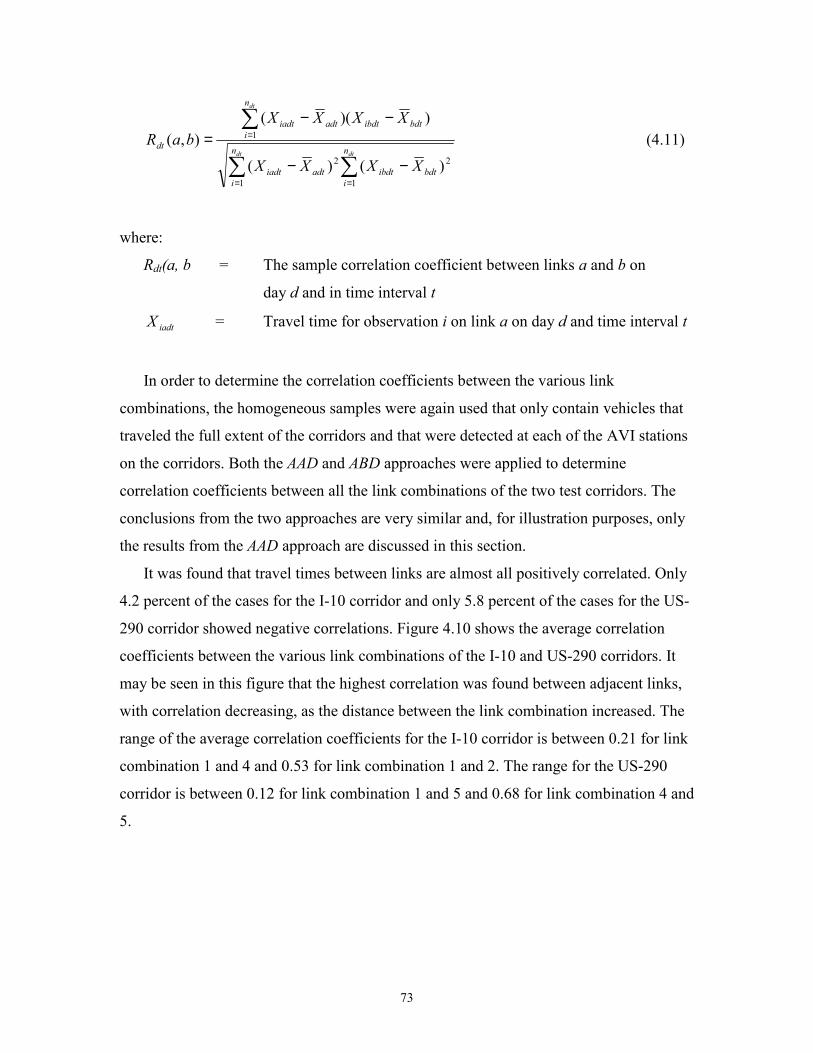
  73

 

∑ ∑

∑

= =

=

−−

−−=

dt dt

dt

n

i

n

ibdtibdtadtiadt

n

ibdtibdtadtiadt

dt

XXXX

XXXXbaR

1 1

22

1

)()(

))((),(         (4.11) 

 

where: 

  Rdt(a, b    =  The sample correlation coefficient between links a and b on  

          day d and in time interval t 

  iadtX     =  Travel time for observation i on link a on day d and time interval t 

 

  In order to determine the correlation coefficients between the various link 

combinations, the homogeneous samples were again used that only contain vehicles that 

traveled the full extent of the corridors and that were detected at each of the AVI stations 

on the corridors. Both the AAD and ABD approaches were applied to determine 

correlation coefficients between all the link combinations of the two test corridors. The 

conclusions from the two approaches are very similar and, for illustration purposes, only 

the results from the AAD approach are discussed in this section. 

  It was found that travel times between links are almost all positively correlated. Only 

4.2 percent of the cases for the I-10 corridor and only 5.8 percent of the cases for the US-

290 corridor showed negative correlations. Figure 4.10 shows the average correlation 

coefficients between the various link combinations of the I-10 and US-290 corridors. It 

may be seen in this figure that the highest correlation was found between adjacent links, 

with correlation decreasing, as the distance between the link combination increased. The 

range of the average correlation coefficients for the I-10 corridor is between 0.21 for link 

combination 1 and 4 and 0.53 for link combination 1 and 2. The range for the US-290 

corridor is between 0.12 for link combination 1 and 5 and 0.68 for link combination 4 and 

5. 

 

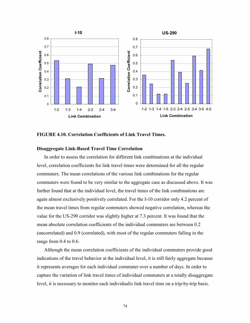
  74

 

FIGURE 4.10. Correlation Coefficients of Link Travel Times.  

Disaggregate Link-Based Travel Time Correlation  

  In order to assess the correlation for different link combinations at the individual 

level, correlation coefficients for link travel times were determined for all the regular 

commuters. The mean correlations of the various link combinations for the regular 

commuters were found to be very similar to the aggregate case as discussed above. It was 

further found that at the individual level, the travel times of the link combinations are 

again almost exclusively positively correlated. For the I-10 corridor only 4.2 percent of 

the mean travel times from regular commuters showed negative correlation, whereas the 

value for the US-290 corridor was slightly higher at 7.3 percent. It was found that the 

mean absolute correlation coefficients of the individual commuters are between 0.2 

(uncorrelated) and 0.9 (correlated), with most of the regular commuters falling in the 

range from 0.4 to 0.6. 

  Although the mean correlation coefficients of the individual commuters provide good 

indications of the travel behavior at the individual level, it is still fairly aggregate because 

it represents averages for each individual commuter over a number of days. In order to 

capture the variation of link travel times of individual commuters at a totally disaggregate 

level, it is necessary to monitor each individualís link travel time on a trip-by-trip basis. 

I-10

0

0.1

0.2

0.3

0.4

0.5

0.6

0.7

0.8

1-2 1-3 1-4 2-3 2-4 3-4

Link Combination

Correlation Coefficient

US-290

0

0.1

0.2

0.3

0.4

0.5

0.6

0.7

0.8

1-2 1-3 1-4 1-5 2-3 2-4 2-5 3-4 3-5 4-5

Link Combination

Correlation Coefficient

  75

This was achieved by comparing each individualís link travel time on a specific day and 

within a specific time interval, with the aggregate estimates for that day and time interval.  

It was found that the link travel times of individual commuters on a trip-by-trip basis are 

not mostly positively correlated as the more aggregate approach suggested. One 

hypothesis for this result is the fact that commuters have certain time budgets for 

traveling a corridor. They would, therefore, compensate by traveling faster on subsequent 

links after experiencing a slow link and vice versa. Another hypothesis is that the slow-

fast pattern along the corridor can be attributed to the effect of shock waves moving up 

and down the corridor during congested conditions. In all likelihood the results are some 

combination of these two effects. 

  More accurate estimates of the link-based speeds and travel times can have 

implications for determining certain sustainability performance measures such as air 

pollution, noise pollution, and fuel consumption. 

 

CONCLUDING REMARKS 

  In this chapter the first phase (identification of performance measures) is performed at 

the corridor level. Various mobility, reliability, air pollution, noise pollution, and energy 

consumption measures were identified.  

  AVI data was used to determine travel time and travel time variability at the level of 

the individual commuter, as well as two levels of aggregation, namely aggregation across 

days (AAD) (i.e., without considering the effect of individual days) and aggregation by 

days (ABD) (i.e., keeping the individual days separate). It was illustrated that corridor 

travel times could be determined with link travel times through the use of a recursive step 

function. The AAD approach was found to be sixty-three percent less accurate than the 

ABD approach for determining individual travel times. Even though the latter technique 

was found to be much more accurate, it was illustrated that forty percent of the regular 

commutersí travel times are statistically different to these aggregate estimates. This result 

has significant implications for sustainability analysis and ATIS applications because 

aggregate estimates of travel time could be significantly different to what is actually 

experienced by a large percentage of commuters. It is, therefore, essential to consider the 

  76

individual level when using ATIS techniques or conducting sustainability analysis at the 

individual level. 

  In the case of travel time variability it was found that the variance of corridor travel 

times could be determined, fairly accurately, using measured link variances and 

covariances when dependence of link travel times is assumed. It was found that for an 

average of approximately twenty percent of the cases the travel time standard deviations 

of the regular commuters are statistically different to the ABD estimates. This result again 

illustrates the benefit of conducting analyses at the level of the individual commuter. 

  On a link basis it was found that travel times between links are almost exclusively 

positively correlated with only five percent of the observations indicating negative 

correlations. Most of the regular commuters show a moderate level of correlation with the 

majority of correlation coefficients for regular commuters falling in the range from 0.4 to 

0.6. The results from analyzing link travel times of individual commuters on a trip-by-trip 

basis, however, revealed that individual commuters show great variability in travel 

behavior as evidenced by the fact that large tendencies to having both faster and slower 

link travel times than the aggregate estimates were observed. The link travel times of 

individual commuters on a trip-by-trip basis are, therefore, not mostly positively 

correlated as the more aggregate approach suggested. More accurate estimates of 

performance measures such as vehicular emissions, noise pollution, and fuel consumption 

can, therefore, be made if analyses are conducted on the individual commuter level and 

on a trip-by-trip basis. 

  It was found that a disaggregate approach will result in superior estimates of travel 

time and travel time variability. This is important because sustainability analyses are to a 

large extent reliant on estimates of these two important performance measures. The 

following chapter describes how mobility related performance measures can be 

quantified at various levels of aggregation by using the TRANSIMS model. 

 

 

  77

CHAPTER 5: MOBILITY RELATED PERFORMANCE MEASURES  

  This chapter focuses on the phases of database development and quantifying 

performance measures. Observed travel information at the level of the individual 

commuter, as can be obtained from AVI data, is often not available or extremely 

expensive to obtain. The planner, therefore, often needs to resort to modeling techniques 

to quantify performance measures for sustainable transportation at a disaggregate level. 

In this chapter, a wide range of mobility and reliability related performance measures are 

quantified at various levels of aggregation by using a traffic simulation model. Various 

traffic simulation models are able to model the travel behavior of the individual 

commuter. However, the TRANSIMS model was selected as simulation model for this 

research because it represents the next generation of planning tools. It has the ability to 

simulate the travel behavior of the individual commuter on a second-by-second basis and, 

therefore, could be used to quantify performance measures for sustainable transportation 

at various levels of aggregation. The CORSIM highway microsimulation model was used 

to confirm some of the results obtained with TRANSIMS. 

 METHODS OF DISAGGREGATION 

  For a typical transportation system, a number of different types of disaggregation can 

be considered, namely spatial, temporal, combined spatial and temporal, and the 

individual level. The individual level can be used as a separate level of disaggregation or 

in combination with spatial and/or temporal disaggregation. Spatial and temporal 

disaggregation can each be applied at different levels of detail, which can be defined by 

the segment lengths and time interval lengths, respectively. Figure 5.1 shows how the 

different types of disaggregation are related. It may be seen in Figure 5.1 that there are 

numerous possible combinations in which the types of disaggregation can be applied. The 

eventual accuracy of the application depends on factors such as the type of 

disaggregation that is applied, the level of detail used within each application, and the 

underlying function of the performance measure that is under analysis. The following 

sections describe the different types of disaggregation in more detail. 

 

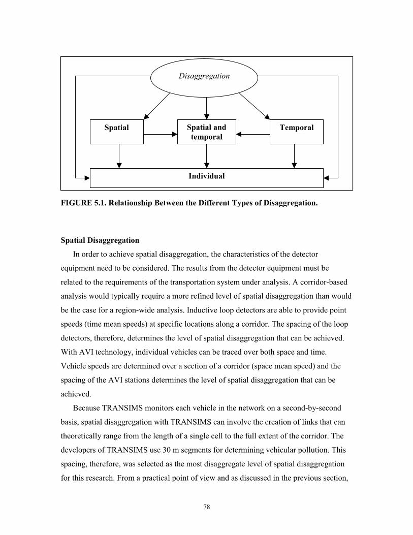
  78

 

 FIGURE 5.1. Relationship Between the Different Types of Disaggregation.  

 

Spatial Disaggregation 

  In order to achieve spatial disaggregation, the characteristics of the detector 

equipment need to be considered. The results from the detector equipment must be 

related to the requirements of the transportation system under analysis. A corridor-based 

analysis would typically require a more refined level of spatial disaggregation than would 

be the case for a region-wide analysis. Inductive loop detectors are able to provide point 

speeds (time mean speeds) at specific locations along a corridor. The spacing of the loop 

detectors, therefore, determines the level of spatial disaggregation that can be achieved. 

With AVI technology, individual vehicles can be traced over both space and time. 

Vehicle speeds are determined over a section of a corridor (space mean speed) and the 

spacing of the AVI stations determines the level of spatial disaggregation that can be 

achieved. 

  Because TRANSIMS monitors each vehicle in the network on a second-by-second 

basis, spatial disaggregation with TRANSIMS can involve the creation of links that can 

theoretically range from the length of a single cell to the full extent of the corridor. The 

developers of TRANSIMS use 30 m segments for determining vehicular pollution. This 

spacing, therefore, was selected as the most disaggregate level of spatial disaggregation 

for this research. From a practical point of view and as discussed in the previous section, 

Spatial  Spatial and temporal 

Temporal 

Individual 

Disaggregation 

  79

the I-10 corridor could be spatially disaggregated into four AVI links or twenty-eight 

interchange links. Similarly, the US-290 corridor could be spatially disaggregated into 

five AVI links and twenty-four interchange links. 

 

Temporal Disaggregation 

  Just as the travel characteristics of a corridor can be spatially disaggregated in terms 

of links, it can also be temporally disaggregated in terms of time intervals. Temporal 

disaggregation with TRANSIMS can involve the creation of time intervals that can 

theoretically range from 1 s to the full extent of the analysis period. For comparison 

purposes, the most disaggregate level of temporal disaggregation was chosen to be 10 s 

intervals. More practical levels of temporal disaggregation could, for example, involve 

the creation of twelve 5-min time intervals or four 15-min time intervals. In the case of 

the test corridors, the highest level of temporal aggregation involves aggregation over the 

whole analysis period. 

 Spatial and Temporal Disaggregation 

  It is also possible to conduct the analysis by disaggregating both spatially and 

temporally. This approach has the potential of considerably reducing the total error as a 

result of aggregation. Joint spatial and temporal disaggregation can also allow the analyst 

to make the necessary trade-offs between aspects such as required accuracy, computing 

time, and memory requirements by selecting the appropriate level of spatial and temporal 

disaggregation. 

 

Disaggregation Based on Individuals 

  Because TRANSIMS can trace the movement of each vehicle in the network, it is 

possible to conduct analyses at the level of the individual vehicle. Another useful aspect 

of data on the individual level is that it lends itself to the determination of mathematical 

or statistical distributions. Histograms were prepared for the mean speeds of the 

individual vehicles on each of the AVI links and for the two test corridors as a whole. 

The shapes of the histograms for the AVI links indicate that the data tend to be normally 

distributed, although fairly long tails to the right were observed for a number of links. 

  80

The Chi-squared distribution with six degrees of freedom was found to be an appropriate 

distribution for individual speed data on the AVI links. 

  On a corridor level the tendency of long tails was less pronounced, and the normal 

distribution seems to be more appropriate. The normal distribution, therefore, can be used 

with caution for approximating individual speed data and for making predictions 

regarding probabilities, percentiles, and confidence intervals. 

 SMOOTHING OF SIMULATED SPEED PROFILES 

  The TRANSIMS model may be classified as a low fidelity model because it has few 

driver decision rules and uses a discrete, cell-based representation of the traffic network. 

In contrast, CORSIM may be considered a high fidelity model because it attempts to 

represent the spatial interaction of drivers on a continuous, rather than a discrete basis 

and because it attempts to model the car-following logic of drivers in detail (90). The 

discrete cell-based nature of TRANSIMS means that vehicles can have instantaneous 

changes in velocity. As mentioned in Chapter 2, a vehicleís speed at any given point in 

time or space is on the range from 0 to 135 km/h in steps of 27 km/h. Each second a 

vehicleís speed is updated and changes of 0 or 27 km/h are applied for acceleration and 0 

to 135 km/h for deceleration. The resulting discrete nature of the individual vehicleís 

speed profile suggests that they may need to be smoothed. 

  There are a number of non-parametric curve-fitting techniques that can be used to 

smooth the individual speed profiles. Some of the best known techniques are smoothing 

splines, kernel estimates, nearest neighbor local polynomials (LOESS) and fixed 

bandwidth local polynomial smoothers (91). 

  These two techniques were compared by using the MAPE metric to compare the 

differences between the smoothed speeds and the simulated speeds, at 1-s intervals. In 

addition to the MAPE metric, the percentage of vehicles that have unrealistic 

accelerations and decelerations were also determined. The uniform kernel technique with 

eleven observations was found to provide the best results under these conditions. This 

approach was used for smoothing speed data from TRANSIMS model. 

  For illustration purposes, Figure 5.2 shows the simulated speed profile for a specific 

vehicle over a 5-min period, as well as the smoothed speed profile as produced by the 

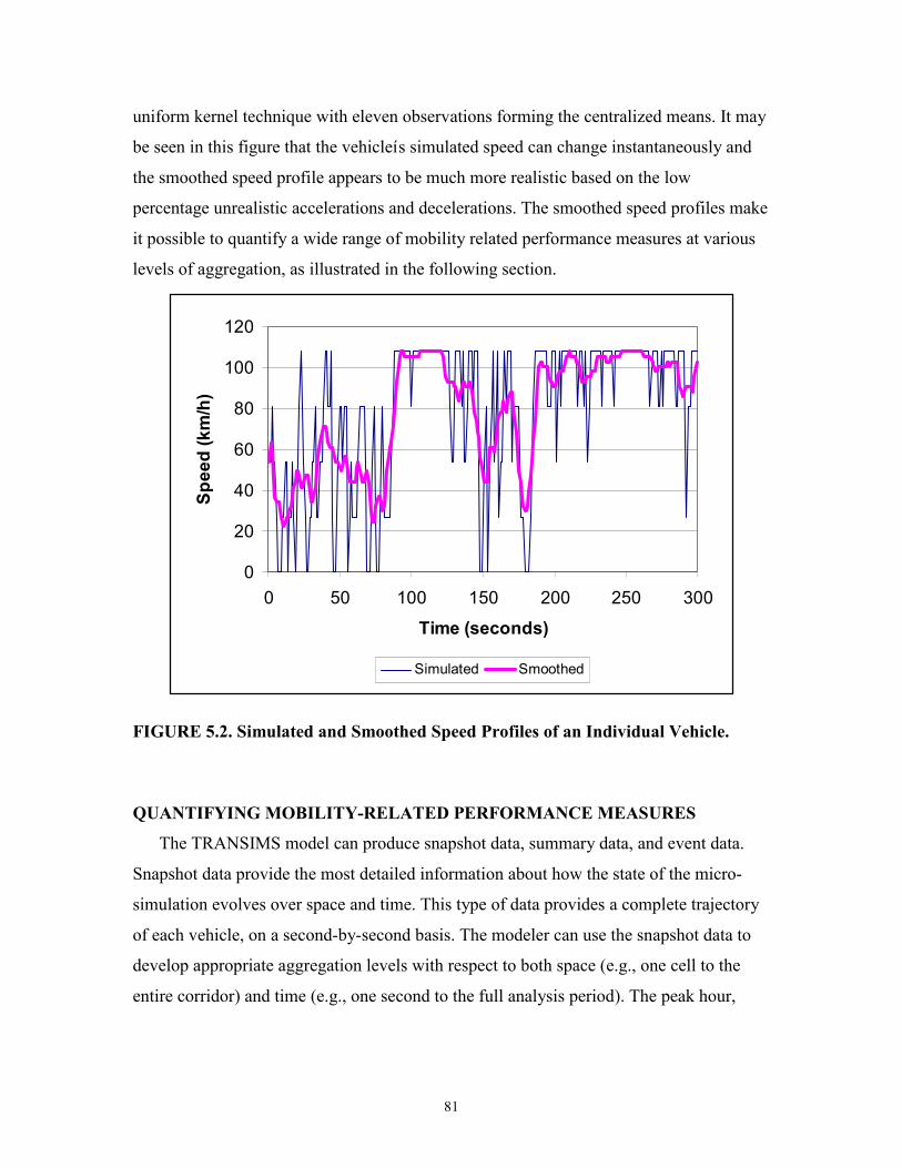
  81

uniform kernel technique with eleven observations forming the centralized means. It may 

be seen in this figure that the vehicleís simulated speed can change instantaneously and 

the smoothed speed profile appears to be much more realistic based on the low 

percentage unrealistic accelerations and decelerations. The smoothed speed profiles make 

it possible to quantify a wide range of mobility related performance measures at various 

levels of aggregation, as illustrated in the following section. 

 

FIGURE 5.2. Simulated and Smoothed Speed Profiles of an Individual Vehicle.  

 

QUANTIFYING MOBILITY-RELATED PERFORMANCE MEASURES 

  The TRANSIMS model can produce snapshot data, summary data, and event data. 

Snapshot data provide the most detailed information about how the state of the micro-

simulation evolves over space and time. This type of data provides a complete trajectory 

of each vehicle, on a second-by-second basis. The modeler can use the snapshot data to 

develop appropriate aggregation levels with respect to both space (e.g., one cell to the 

entire corridor) and time (e.g., one second to the full analysis period). The peak hour, 

0

20

40

60

80

100

120

0 50 100 150 200 250 300

Time (seconds)

Speed (km/h)

Simulated Smoothed

  82

which lasted from 7 a.m. to 8 a.m., was selected as analysis period with the TRANSIMS 

model. 

  It was shown in Chapter 3 that traffic simulation models could be used to quantify 

performance measures that address the sustainable transportation goals of maximizing 

reliability and maximizing mobility. The TRANSIMS model is used to quantify the 

reliability performance measure, namely travel time variability and the following 

mobility related performance measures: i) travel time; ii) total delay; iii) travel rate; iv) 

level of service; and v) percentage corridor congested. It was found that spatial 

disaggregation at the level of interchange links and the temporal disaggregation at 5-min 

time increments are both practical and fairly accurate levels for quantifying performance 

measures. Both these levels of aggregation resulted in an eighty percent improvement in 

speed estimation over the completely aggregate cases. These levels of disaggregation, as 

well as the smoothed speed profiles, were, therefore, used for quantifying the various 

mobility and reliability related performance measures. 

 

Travel Time 

  As discussed in Chapter 4, travel time is a very important performance measure for 

sustainable transportation analysis. It can be measured on a link basis, as well as over the 

full extent of the corridor. The travel time over the full extent of the corridor is often of 

most interest as a performance measure for sustainable transportation and can be 

calculated by recording the difference between the corridor exiting and entering times as 

shown in Equation 5.1. 

 

Corridor travel time =  entryexit tt −             (5.1) 

 

  Figure 5.3 shows the mean travel times for the various corridor entering time 

intervals. It may be seen in Figure 5.3 that the mean travel time for the I-10 corridor 

shows an increasing trend, with the maximum travel time being reached at a corridor 

entering time that occurs just before 8 a.m. The trend for the US-290 corridor, however, 

is slightly decreasing over this period. 

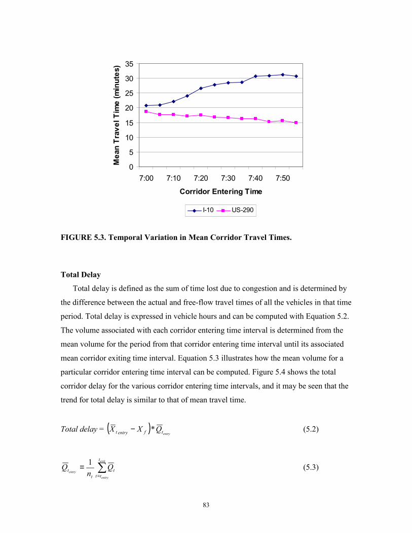
  83

 

FIGURE 5.3. Temporal Variation in Mean Corridor Travel Times.  

 

Total Delay 

  Total delay is defined as the sum of time lost due to congestion and is determined by 

the difference between the actual and free-flow travel times of all the vehicles in that time 

period. Total delay is expressed in vehicle hours and can be computed with Equation 5.2. 

The volume associated with each corridor entering time interval is determined from the 

mean volume for the period from that corridor entering time interval until its associated 

mean corridor exiting time interval. Equation 5.3 illustrates how the mean volume for a 

particular corridor entering time interval can be computed. Figure 5.4 shows the total 

corridor delay for the various corridor entering time intervals, and it may be seen that the 

trend for total delay is similar to that of mean travel time. 

 

Total delay =  ( )entrytfentryt QXX *−             (5.2) 

 

∑=

=exit

entry

entry

t

ttt

tt Q

nQ 1                 (5.3) 

0

5

10

15

20

25

30

35

7:00 7:10 7:20 7:30 7:40 7:50

Corridor Entering Time

Mean Travel Time (minutes)

I-10 US-290

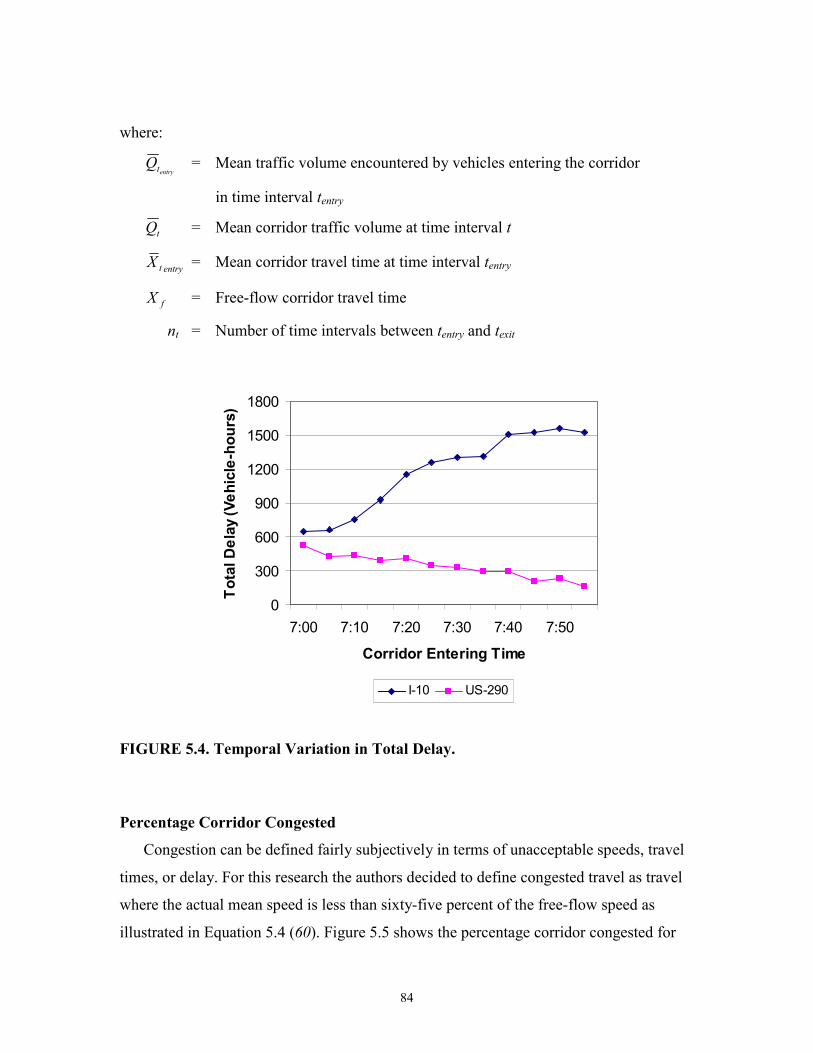
  84

 

where: 

 entrytQ   =  Mean traffic volume encountered by vehicles entering the corridor 

        in time interval tentry 

  tQ     =  Mean corridor traffic volume at time interval t 

  entrytX  =  Mean corridor travel time at time interval tentry 

  fX   =  Free-flow corridor travel time 

    nt   =  Number of time intervals between tentry and texit 

 

FIGURE 5.4. Temporal Variation in Total Delay.  

 

Percentage Corridor Congested 

  Congestion can be defined fairly subjectively in terms of unacceptable speeds, travel 

times, or delay. For this research the authors decided to define congested travel as travel 

where the actual mean speed is less than sixty-five percent of the free-flow speed as 

illustrated in Equation 5.4 (60). Figure 5.5 shows the percentage corridor congested for 

0

300

600

900

1200

1500

1800

7:00 7:10 7:20 7:30 7:40 7:50

Corridor Entering Time

Total Delay (Vehicle-hours)

I-10 US-290

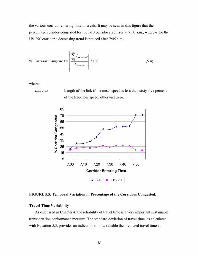
  85

the various corridor entering time intervals. It may be seen in this figure that the 

percentage corridor congested for the I-10 corridor stabilizes at 7:50 a.m., whereas for the 

US-290 corridor a decreasing trend is noticed after 7:45 a.m. 

 

% Corridor Congested =  100*1

∑

=

corridor

n

lcongested

L

Ll

        (5.4) 

 

where: 

  Lcongested   =  Length of the link if the mean speed is less than sixty-five percent 

          of the free-flow speed, otherwise zero. 

 

FIGURE 5.5. Temporal Variation in Percentage of the Corridors Congested.  

Travel Time Variability 

  As discussed in Chapter 4, the reliability of travel time is a very important sustainable 

transportation performance measure. The standard deviation of travel time, as calculated 

with Equation 5.5, provides an indication of how reliable the predicted travel time is. 

5

1525

3545

55

6575

85

7:00 7:10 7:20 7:30 7:40 7:50

Corridor Entering Time

% Corridor Congested

I-10 US-290

  86

Comparisons between links can be performed with the coefficient of variation, which can 

be computed with Equation 5.6. Figure 5.6 shows the travel time standard deviations for 

the various corridor entering time intervals, as well as the coefficients of variation for the 

different links. It may be seen in this figure that the travel time variability shows great 

variation both spatially and temporally with the I-10 corridor showing the greatest travel 

time variability. 

 

  Sct =  [ ]∑=

−−

tn

jctjct

t

XXn 1

2

)1(1     (5.5) 

 

 lt

ltlt X

SCV =     (5.6) 

 

where: 

  Sct    =  Corridor travel time standard deviation at time interval t 

  Slt     =  Travel time standard deviation for link l at time interval t 

  CVlt  =  Coefficient of variation for link l and at time interval t 

  Xjct   =  Corridor travel time for vehicle j at time interval t  

  ctX   =  Mean corridor travel time at time interval t 

  ltX   =  Mean travel time for link l at time interval t 

 

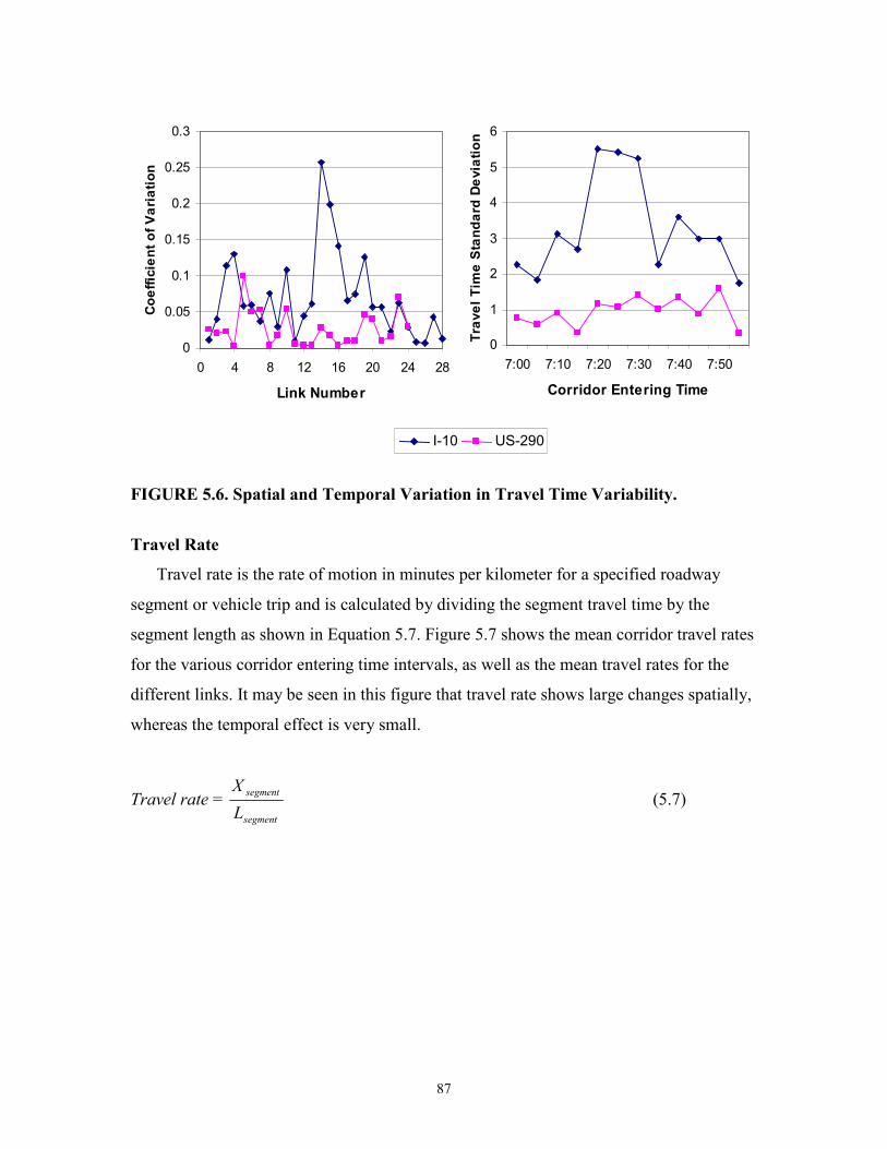
  87

 

FIGURE 5.6. Spatial and Temporal Variation in Travel Time Variability.  

Travel Rate 

  Travel rate is the rate of motion in minutes per kilometer for a specified roadway 

segment or vehicle trip and is calculated by dividing the segment travel time by the 

segment length as shown in Equation 5.7. Figure 5.7 shows the mean corridor travel rates 

for the various corridor entering time intervals, as well as the mean travel rates for the 

different links. It may be seen in this figure that travel rate shows large changes spatially, 

whereas the temporal effect is very small. 

 

Travel rate = segment

segment

LX

               (5.7) 

 

0

1

2

3

4

5

6

7:00 7:10 7:20 7:30 7:40 7:50

Corridor Entering Time

Travel Time Standard Deviation

0

0.05

0.1

0.15

0.2

0.25

0.3

0 4 8 12 16 20 24 28

Link Number

Coefficient of Variation

I-10 US-290 

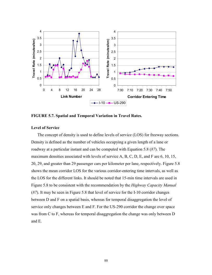
  88

 

FIGURE 5.7. Spatial and Temporal Variation in Travel Rates.  

Level of Service 

  The concept of density is used to define levels of service (LOS) for freeway sections. 

Density is defined as the number of vehicles occupying a given length of a lane or 

roadway at a particular instant and can be computed with Equation 5.8 (87). The 

maximum densities associated with levels of service A, B, C, D, E, and F are 6, 10, 15, 

20, 29, and greater than 29 passenger cars per kilometer per lane, respectively. Figure 5.8 

shows the mean corridor LOS for the various corridor-entering time intervals, as well as 

the LOS for the different links. It should be noted that 15-min time intervals are used in 

Figure 5.8 to be consistent with the recommendation by the Highway Capacity Manual 

(87). It may be seen in Figure 5.8 that level of service for the I-10 corridor changes 

between D and F on a spatial basis, whereas for temporal disaggregation the level of 

service only changes between E and F. For the US-290 corridor the change over space 

was from C to F, whereas for temporal disaggregation the change was only between D 

and E. 

 

0

0.5

1

1.5

2

2.5

3

3.5

4

7:00 7:10 7:20 7:30 7:40 7:50

Corridor Entering Time

Travel Rate (minutes/km)

0

0.5

1

1.5

2

2.5

3

3.5

4

0 4 8 12 16 20 24 28

Link Number

Travel Rate (minutes/km)

I-10 US-290 

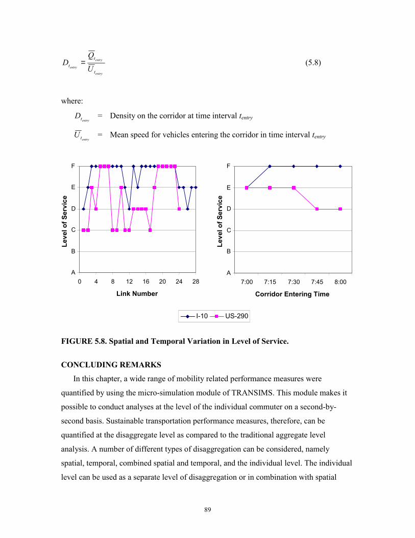
  89

entry

entry

entryt

tt U

QD =                   (5.8) 

 

where: 

 entrytD   =  Density on the corridor at time interval tentry 

 entrytU   =  Mean speed for vehicles entering the corridor in time interval tentry 

 

FIGURE 5.8. Spatial and Temporal Variation in Level of Service.  

CONCLUDING REMARKS 

  In this chapter, a wide range of mobility related performance measures were 

quantified by using the micro-simulation module of TRANSIMS. This module makes it 

possible to conduct analyses at the level of the individual commuter on a second-by-

second basis. Sustainable transportation performance measures, therefore, can be 

quantified at the disaggregate level as compared to the traditional aggregate level 

analysis. A number of different types of disaggregation can be considered, namely 

spatial, temporal, combined spatial and temporal, and the individual level. The individual 

level can be used as a separate level of disaggregation or in combination with spatial 

I-10  US-290

A

B

C

D

E

F

7:00 7:15 7:30 7:45 8:00

Corridor Entering Time

Level of Service

A

B

C

D

E

F

0 4 8 12 16 20 24 28

Link Number

Level of Service

  90

and/or temporal disaggregation. Spatial and temporal disaggregation can each be applied 

at different levels of detail, which can be defined by the segment lengths and time 

interval lengths, respectively. These types of disaggregation, as well as the resolution of 

each dimension, can be changed to allow the analyst to make various trade-offs between 

accuracy, computing time, and memory requirements. 

  It was shown that disaggregation based on individuals improved the accuracy with 

which performance measures were quantified and made it possible to determine statistical 

distributions for parameters such as speed and travel time. The Chi-squared distribution 

was found to be an appropriate distribution for individual speed data on the AVI links, 

whereas the normal distribution showed more promise for individual speed data on the 

corridor level. 

  The discrete cell-based nature of TRANSIMS means that vehicles can have 

instantaneous changes in velocity, resulting in seemingly erratic speed profiles. It was 

found that a uniform kernel estimator can be used to smooth the individual speed profiles 

produced by the TRANSIMS micro-simulator. These smoothed speed profiles were used 

to quantify mobility related performance measures at various levels of spatial and 

temporal disaggregation. It was again found that spatial disaggregation can considerably 

improve the accuracy with which performance measures of sustainable transportation are 

quantified. 

  The quantified performance measures are used as input into the multi-criteria 

decision-making process and the index for sustainable transportation as will be discussed 

in Chapter 7. The following chapter discusses how environmentally related performance 

measures can be quantified by using output from the TRANSIMS model, as well as 

various transportation environmental impact models. 

 

 

 

  91

CHAPTER 6: ENVIRONMENTAL RELATED PERFORMANCE 

MEASURES  

  This chapter focuses on the phases of database development and quantifying 

performance measures. As discussed in Chapter 3, the environment is one of the three 

dimensions of sustainable transportation. In this chapter, environmental related 

performance measures, namely vehicular emissions, noise pollution, and fuel 

consumption are quantified at various levels of aggregation. Output from the micro- 

simulator TRANSIMS, as well as a number of transportation environmental impact 

models, are used to quantify the performance measures. 

 

AIR POLLUTION 

Preparation of the Emission Model 

  For this research, the MOBILE 5a vehicular emission model developed by the EPA 

was used. The reason for using MOBILE 5a is that it is currently the state of the practice 

in Texas and also in most of North America. The basic emission rates are determined 

through actual vehicle tests on an apparatus called a dynamometer, which consists of a 

large chassis with a roller under which the drive wheels of the vehicle are placed. The 

roller applies forces to the drive wheels to simulate the loading experienced in actual 

driving conditions. Vehicles are driven through cycles on the dynamometer that are 

designed to be indicative of driving patterns in urban areas. Emissions for various vehicle 

classes, model years, and operating conditions are recorded with special measuring 

equipment. Basic emission rate equations are then developed for each pollutant, vehicle 

type, model year, as well as emission standards and the emission control technologies 

used (82,84). 

  The MOBILE 5a model can, therefore, be used to determine emissions from the 

operating conditions of individual vehicles on a second-by-second basis. Because 

traditional transportation planning models produce mean speeds for groups of vehicles, 

the MOBILE 5a model is generally not applied at this level of disaggregation. The 

TRANSIMS model, however, can produce this type of disaggregate information. Based 

on the illustrations in Chapter 5 that disaggregate information can provide more accurate 

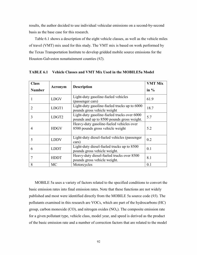
  92

results, the author decided to use individual vehicular emissions on a second-by-second 

basis as the base case for this research. 

  Table 6.1 shows a description of the eight vehicle classes, as well as the vehicle miles 

of travel (VMT) mix used for this study. The VMT mix is based on work performed by 

the Texas Transportation Institute to develop gridded mobile source emissions for the 

Houston-Galveston nonattainment counties (92). 

 

TABLE 6.1  Vehicle Classes and VMT Mix Used in the MOBILE5a Model  

Class 

Number Acronym  Description 

VMT Mix 

in % 

1  LDGV  Light-duty gasoline-fueled vehicles (passenger cars)  61.9 

2  LDGT1  Light-duty gasoline-fueled trucks up to 6000 pounds gross vehicle weight  18.7 

3  LDGT2  Light-duty gasoline-fueled trucks over 6000 pounds and up to 8500 pounds gross weight.  5.7 

4  HDGV Heavy-duty gasoline-fueled vehicles over 8500 pounds gross vehicle weight  

5.2 

5  LDDV  Light-duty diesel-fueled vehicles (passenger cars)  0.2 

6  LDDT  Light-duty diesel-fueled trucks up to 8500 pounds gross vehicle weight.  0.1 

7  HDDT  Heavy-duty diesel-fueled trucks over 8500 pounds gross vehicle weight.  8.1 

8  MC  Motorcycles  0.1  

 

  MOBILE 5a uses a variety of factors related to the specified conditions to convert the 

basic emission rates into final emission rates. Note that these functions are not widely 

published and most were identified directly from the MOBILE 5a source code (93). The 

pollutants examined in this research are VOCs, which are part of the hydrocarbons (HC) 

group, carbon monoxide (CO), and nitrogen oxides (NOx). The composite emission rate 

for a given pollutant type, vehicle class, model year, and speed is derived as the product 

of the basic emission rate and a number of correction factors that are related to the model 

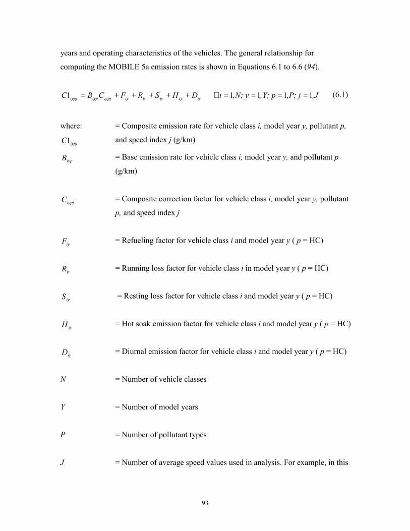
  93

years and operating characteristics of the vehicles. The general relationship for 

computing the MOBILE 5a emission rates is shown in Equations 6.1 to 6.6 (94). 

 

,J,P; j,Y; p,N; yiDHSRFCBC iyiyiyiyiyiypjiypiypj 1111       1 ====∀+++++=  

 

(6.1) 

where: 

iypjC1  

= Composite emission rate for vehicle class i, model year y, pollutant p, 

and speed index j (g/km)  

iypB   = Base emission rate for vehicle class i, model year y, and pollutant p 

(g/km)  

 

iypjC   = Composite correction factor for vehicle class i, model year y, pollutant 

p, and speed index j  

 

iyF   = Refueling factor for vehicle class i and model year y ( p = HC) 

 

iyR   = Running loss factor for vehicle class i in model year y ( p = HC)  

 

iyS    = Resting loss factor for vehicle class i and model year y ( p = HC)  

 

iyH   = Hot soak emission factor for vehicle class i and model year y ( p = HC)  

 

iyD   = Diurnal emission factor for vehicle class i and model year y ( p = HC)  

 

N  = Number of vehicle classes  

 

Y  = Number of model years 

 

P  = Number of pollutant types 

 

J  = Number of average speed values used in analysis. For example, in this 

  94

research the average speeds ranged from 4.8 km/h to 104 km/h in 

increments of 1.6 km/h (1 mi/h) then J = 63 and the speed associated with 

speed index j = 10 would be 19.2 km/h. 

 

  It should be noted that the evaporative factors related to HC emissions in Equation 

6.1 are often given in gram per unit time rather than g/km. These factors, therefore, need 

to be converted in order to obtain the desired emission rate. In addition, ambient 

temperature and Reid vapor pressure (RVP) also affect the emission rate. The details of 

these effects are beyond the scope of this report but may be identified directly from the 

MOBILE 5a source code. 

  The composite correction factor for a given vehicle class i, model year y, pollutant p, 

and speed index j is calculated as shown in Equation 6.2. 

,Jj,P;  ,Y;  p y ,N; iHTALVMS

C iypiypiypiypiypiy

iypsiypj 111 1              =∀==∀=∀=   (6.2) 

where: 

iypjS  

= Speed correction factor for vehicle class i, model year y, pollutant p, and 

speed index j  

 

iyM   = Cold start/ hot start adjustment factor for vehicle class i, and model year y  

 

iypV   = Fuel volatility factor for vehicle class i, model year y, and pollutant p  

 

iypL   = Loading factor for vehicle class i, model year y, and pollutant p  

 

iypA   = Air conditioning factor for vehicle class i, model year y, and pollutant p 

 

iypT   = Trailer towing factor for vehicle class i, model year y, and pollutant p 

 

iypH   = Humidity factor for vehicle class i, model year y, and pollutant p (p= NOX) 

  

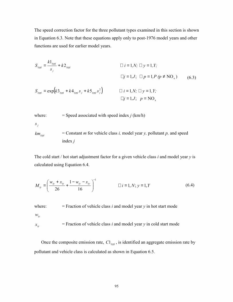
  95

The speed correction factor for the three pollutant types examined in this section is shown 

in Equation 6.3. Note that these equations apply only to post-1976 model years and other 

functions are used for earlier model years. 

 

( )x

2

x

NO   ;1                                                                           11               543exp

)NO1 ;1                                                                           

11                                           21

==∀

=∀=∀++=

≠=∀=∀

=∀=∀+=

p,Jj,Y;   y,N;  iskskkS

,P (p p ,Jj

,Y;   y,N;  iksk

S

jiypjjiypjiypjiypj

iypjj

iypjiypj

 

 

 

 

(6.3) 

where: 

js  

= Speed associated with speed index j (km/h) 

 

iypjkm   = Constant m for vehicle class i, model year y, pollutant p, and speed 

index j  

 

The cold start / hot start adjustment factor for a given vehicle class i and model year y is 

calculated using Equation 6.4. 

 

YyNixwxw

M iyiyiyiyiy ,1 ;,1                    

161

26

1

==∀

−−+

+=

−

 

 

(6.4) 

where: 

iyw  

= Fraction of vehicle class i and model year y in hot start mode 

 

iyx   = Fraction of vehicle class i and model year y in cold start mode 

 

  Once the composite emission rate,  iypjC1 , is identified an aggregate emission rate by 

pollutant and vehicle class is calculated as shown in Equation 6.5. 

 

  96

JjPpNizCCY

yiyjiypjipj ,1 ;,1  ;,1              12

1

===∀=∑=

  (6.5) 

where: 

ipjC2  

= Composite emission rate for vehicle class i, pollutant p, and speed index 

j (g/km) 

 

iyjz   = Fraction of total VKT for vehicle class i contributed by model year y for 

speed index j 

 

 

  It is important to note that emissions on a g/s basis are not calculated in the MOBILE 

5a model. A long section of highway with a high average speed may have the same 

overall level of pollutant emissions as a shorter section of highway with a low average 

speed, all else being equal. The emission rates are developed in terms of grams of 

pollutant per distance traveled, because vehicle kilometers of travel (VKT) and average 

speed per link can be obtained from the output of transportation planning models. The 

total amount of pollutant p emitted in a given traffic network can, therefore, readily be 

calculated by summing the product of the emission rate and the VKT for each vehicle 

class (categorized by average speed) as shown in Equation 6.6.  

 

∑∑= =

=∀=N

i

J

jijipjp PpvCT

1 1

,1            2  

 

(6.6) 

where: 

ijv  

= Vehicle kilometers of travel for vehicle class i traveling at the speed 

associated with speed index j. Note that the VKT implicitly assumes a 

time unit (i.e. per month, per year) 

 

pT   = Total amount of pollutant p produced (g). Note that this is expressed 

in the same units (i.e. per month, per year) as  ijv .  

 

  Given the eight vehicle classifications, three pollutants, fifty model years, and the 

large number of causal variables, the task of writing out all of the equations in the 

  97

MOBILE 5a model would be quite burdensome. Consequently a computer program has 

been written to perform the calculations for the analyst. 

  While the emission rates used in Equation 6.6 are calculated for an individual test 

vehicle traveling at an average speed, there is no standard protocol for identifying the 

VKT for each vehicle class i and speed j ( ijv ). Typically, a macroscopic four-step 

transportation model is used to identify  ijv  and there are three important points related to 

this fact. The first is that for a given link the recorded VKT by vehicle class is based on 

an average speed for all vehicle classes because only one speed value per link is output. 

Secondly, there are no specifications on the appropriate link length or time interval for 

analyses purposes. This potentially could be problematic because the average speed used 

in Equation 6.2 will be a function of the temporal and spatial aggregation length used to 

calculate the average speed. Thirdly, if a network is small, has low volumes of vehicle 

class i (i.e., one unit per time period for a given speed), and if the spatial and temporal 

analysis units were small enough, the net effect would be to run MOBILE 5a at a totally 

disaggregate level. 

  The first issue discussed above may be illustrated best by the following example. 

Consider a 1 km section of roadway that is being analyzed over a given time period. Two 

heavy-duty diesel vehicles (HDDT) traverse the link at an average speed of 60 and 80 

km/h, respectively, and two light-duty gasoline fueled vehicles (LDGV) traverse the link 

at an average speed of 70 and 90 km/h, respectively. The simplest approach, and that 

adopted in most macroscopic models, would be to assign each vehicle class an average 

speed of 75 km/h, even though no vehicle class experiences this average speed. This will 

be referred to as Scenario 1 in this section. 

  The first issue may be obviated through the use of a micro-simulation model. For 

example, the VKT of the HDDT class would be 2 km at an average speed of 70 km/h and 

the VKT of the LDGV class would be 2 km at an average speed of 80 km/h. Note that 

none of the vehicles actually experienced these average speeds over the roadway section. 

By extending this concept further, the emission rates could be calculated at an even more 

disaggregate level. That is, the emission rate for each vehicle on a particular section of 

roadway could be calculated based on the average speed experienced by each vehicle 

rather than the average speed of all the vehicles belonging to that vehicle class. For 

  98

example, the HDDT would have one VKT at an average speed of 60 km/h and one VKT 

at an average speed of 80 km/h, as opposed to the two VKT at an average speed of 70 

km/h. This approach will be referred to as Scenario 2 in this section. 

  The relationship between emission estimates and the time interval and distance used 

in the analyses are unclear. Identifying this relationship will be the focus of the remainder 

of the section by examining how different aggregation levels can affect emission 

estimates. It is important to note that the goal is not to recommend a specific aggregation 

policy but to show how the trade-offs can be examined and to quantify these trade-offs on 

a real test bed. 

 

Sensitivity Analysis of Emissions Estimates 

  It was found that, in general, MOBILE 5a emission rates are: i) relatively high at low 

average speeds; ii) decrease at a decreasing rate as the average speed increases; and iii) 

then, after a threshold average speed, begin to increase again. If the emission rates were a 

linear function of average speed then aggregation size would have no effect on the overall 

results.  However, because emission rates have an inherently non-linear profile, the 

aggregation effect needs to be examined. This point may be illustrated best by example. 

  Consider a 1 km link that is being analyzed over three consecutive 20-min periods. 

There are 100 LDGV vehicles in each 20-min period and the average speed experienced 

on the link in the three periods are 60, 80, and 100 km/h. The corresponding emission 

rates for VOC as produced by the MOBILE 5a model for the Houston test bed are: 

0.6998; 0.5728; and 0.7353 g/km for the 60, 80 and 100 km/h speeds, respectively. If the 

analysis was performed for each 20-min period, the total estimated VOC emissions using 

Equation 6.6 would be 200.8 g. However, if the analysis was performed over 1 h, the 

three 100 VKT for LDGV vehicles would have an average travel speed of 80 km/h and 

the estimated total VOC emissions would be 171.8 g. In order to predict the magnitude of 

this difference and whether it would be positive or negative, detailed information on the 

emission functions would be required. More importantly, because there are no clear 

guidelines provided on how to calculate the VKT (vij) in Equation 6.6, it would be 

impossible to state which aggregation level gives the best results. All that can be shown 

are the relative differences in emission estimates for different scenarios, which is the goal 

  99

of the sensitivity analyses performed in the next section. 

 

Spatial and Temporal Disaggregation 

  The sensitivity of the emission estimates to spatial aggregation was analyzed by 

varying the segment length from 30 m to that of the base links. The full peak hour was 

used as the analysis period. The sensitivity of the emission estimates to temporal 

aggregation was analyzed by varying the analysis time intervals from 10s to 60 min. 

Additionally, the temporal analysis was performed on the base link level. 

  For each level of temporal and spatial aggregation described above, the total emission 

estimates for the corridor were calculated using the previously described Scenarios 1 and 

2. In the case of Scenario 1, the average speed and total distance traveled for all vehicles 

in each vehicle class were determined for each spatial and temporal aggregation level. 

The average speed along with the VKT per vehicle class was then used to estimate vij in 

Equation 6.6. In the case of Scenario 2, the average speed and distance traveled of each 

individual vehicle within each vehicle class were determined for each spatial and 

temporal aggregation level. The average speed and VKT of each vehicle were used to 

estimate vij. The total emissions determined with each scenario were then compared to the 

base case and the real percentage deviations from the base are shown in Figure 6.1. 

 

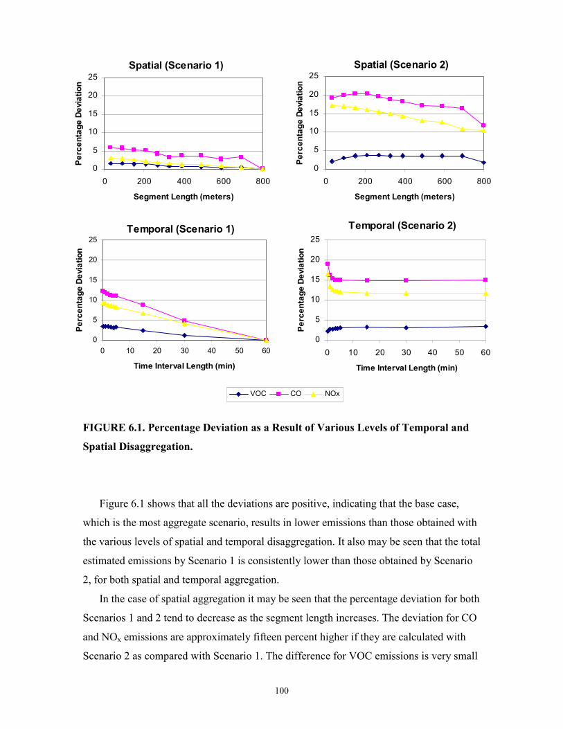
  100

 

FIGURE 6.1. Percentage Deviation as a Result of Various Levels of Temporal and 

Spatial Disaggregation. 

 

 

  Figure 6.1 shows that all the deviations are positive, indicating that the base case, 

which is the most aggregate scenario, results in lower emissions than those obtained with 

the various levels of spatial and temporal disaggregation. It also may be seen that the total 

estimated emissions by Scenario 1 is consistently lower than those obtained by Scenario 

2, for both spatial and temporal aggregation. 

  In the case of spatial aggregation it may be seen that the percentage deviation for both 

Scenarios 1 and 2 tend to decrease as the segment length increases. The deviation for CO 

and NOx emissions are approximately fifteen percent higher if they are calculated with 

Scenario 2 as compared with Scenario 1. The difference for VOC emissions is very small 

VOC CO  NOx 

Temporal (Scenario 2)

0

5

10

15

20

25

0 10 20 30 40 50 60

Time Interval Length (min)

Percentage Deviation

Temporal (Scenario 1)

0

5

10

15

20

25

0 10 20 30 40 50 60

Time Interval Length (min)

Percentage Deviation

Spatial (Scenario 2)

0

5

10

15

20

25

0 200 400 600 800

Segment Length (meters)

Percentage

 Deviation

Spatial (Scenario 1)

0

5

10

15

20

25

0 200 400 600 800

Segment Length (meters)

Percentage

 Deviation

  101

(less than three percent). It may also be seen in Figure 6.1 that for both Scenarios 1 and 2, 

as the segment length increases, the percentage deviation from the base case decreases. 

  In the case of temporal aggregation, it may be seen that Scenario 1 is much more 

susceptible for time interval changes than Scenario 2. In the case of Scenario 1 the 

percentage deviation decreases as the time interval length increases. For Scenario 2 the 

percentage deviation remains nearly constant regardless of the interval length used. In the 

case of CO emissions, for example, the difference between Scenario 1 and Scenario 2 at 

5-min intervals is approximately five percent, whereas the difference at 60-min intervals 

is fifteen percent. 

  It can be concluded that for this test corridor, larger emission estimates will be 

obtained if Scenario 2 is used as opposed to Scenario 1. Therefore, if the hypothesis is 

true that Scenario 2 is more accurate than Scenario 1, the total emissions for the test 

corridor is higher than what is estimated through the conventional approach. 

 

Combined Spatial and Temporal Disaggregation 

  A comparison was performed for combined spatial and temporal disaggregation. Four 

time intervals 10, 60, 120, and 300 s, were used in combination with four segment 

lengths 30, 180, and 360 m and the base links. The total vehicular emission for each of 

the three pollutant types, therefore, could be determined for sixteen combinations of 

spatial and temporal disaggregation and for both Scenarios 1 and 2. 

  It was found that the deviations from the base case for Scenarios 1 and 2 are very 

similar and exclusively positive. Carbon monoxide had the greatest deviation from the 

base case at twenty percent when 30 m segments were combined with 10-s intervals. 

Volatile organic compounds showed the smallest deviation at less than two percent when 

the base links were combined with 5-min intervals. Additionally, it was found that for 

fixed spacings the size of the time increment made hardly any difference (less than two 

percent), whereas for fixed time increments the segment lengths made a more noticeable 

difference (up to ten percent). 

  A test was conducted to determine emission estimates at the totally disaggregate 

level, namely for each vehicle on a second-by-second basis. Although MOBILE 5a was 

never intended to be used in this way, it is interesting to notice that the emissions 

  102

produced by this totally disaggregate approach were within one percent of that obtained 

with Scenario 2 at 10-s intervals and 30 m segments. 

 

Memory Efficiency 

  It can be expected that highly disaggregate data sets produced by micro-simulation 

models and ITS applications can result in very high memory requirements and slow 

computing times. For example, TRANSIMS produced approximately ten million lines of 

data for the I-10 corridor during the peak hour, requiring approximately 500 megabytes 

of memory. 

  By aggregating the micro-simulation data spatially and/or temporally, considerable 

reduction in the total number of observations can be achieved. For example, in the case of 

Scenario 2, a six-fold reduction in data archiving requirements can be achieved when 90 

m segments are used and a ten-fold reduction when 10-s intervals are used, as compared 

with the second-by-second micro-simulation data.  

Sensitivity Analysis with ITS Data 

  Traffic data as produced by ITS applications are sometimes used as input into 

emissions models such as MOBILE 5a (95). These data, however, are typically collected 

and stored at varying levels of spatial and temporal aggregation. Additionally, with some 

forms of ITS data it is also possible to keep track of the individual vehicles. 

  TRANSIMS was used to simulate output from loop detectors, AVI technology, and 

AVL technology. For comparison purposes, only the LDGV vehicle type was considered. 

Equation 6.6 was used to determine the total emissions based on data produced by the 

various types of ITS applications. The peak hour was used as the time interval and the 

base links were used as segments. The only difference between the various calculations is 

in the determination of  ijv  (VKT for the LDGV vehicles traveling at speed index j). The 

most aggregate application (output from the conventional transportation planning model) 

was again selected as the base case. 

 

  103

Loop Detectors 

  The most aggregate form of ITS data considered in this analysis is from inductive 

loop detectors. In order to simulate the loop detectors, detection areas of 40 m in length 

were created before each point where the on- and off-ramps connect with the mainline of 

the freeway. Forty-meter detection areas were used because the maximum simulated 

velocity of a vehicle is 37.5 m/s and the 40 m length ensures that no vehicle will cross it 

undetected. The detection was performed by recording the time and location of the first 

observation of each vehicle within the detection area. 

  The average space mean speed of a given link was assumed to be equal to the average 

instantaneous or time mean speed measured at the loop detectors at the end of the link. 

The VKT was calculated based on the link length and measured volume. Note that due to 

the aggregate nature of link detectors only Scenario 1 could be modeled. 

  It was found that the differences in total emissions calculated with loop detector data 

were zero, twelve, and six percent for VOC, CO, and NOx emissions, respectively. The 

primary reason for the differences is that the speeds from loop detectors are based on 

time mean speed while those for the base case are based on space mean speed. 

 

Automatic Vehicle Identification (AVI) Technology 

  Automatic vehicle identification data were simulated by matching the individual 

vehicles from detection area to detection area, and by determining their mean speeds 

based on the difference in detection times and the spatial separation of the detection 

areas. Given the link travel time and link speed, the average speed of each vehicle 

traversing the link (space mean speed) was determined. These speeds could either be 

averaged across all vehicles in the LDGV class (Scenario 1) or kept separate (Scenario 

2). Because Scenario 1 is equal to the base case, only the application of Scenario 2 will 

be discussed in this section. 

  The VKT is determined by considering the link length and the number of vehicles 

matched at the beginning and end of the links. With this approach a fifteen percent under-

reporting was noticed due to vehicles entering the main lanes downstream of a detection 

area and, therefore, not being detected on that link. This under-reporting was adjusted 

  104

using a factor representing the ratio of the simulated volume for that link and the number 

of matches recorded. 

  The differences in total emission rates, as compared with the base case, of six, 

eighteen, and fourteen percent were obtained for VOC, CO, and NOx emissions, 

respectively. These differences, however, are within five percent of what was obtained 

with Scenario 2 applied at 60 min and for the base links. The AVI results are slightly 

different from this scenario due to the necessary adjustments made because of the under-

reporting in the AVI data, whereas with the regular simulation data the VKT and speed of 

all the vehicles on the network could be determined. 

 

Automatic Vehicle Location (AVL) Technology 

  By keeping track of each vehicleís speed and location on a second-by-second basis, 

AVL data can be simulated. The assumption made for AVL technology is that all 

vehicles in the network may be detected on a second-by-second basis. In the case of AVL 

data, the instantaneous speed and distance traveled by each vehicle on a second-by-

second basis was used for determining  ijv . 

  It was found that the total emissions calculated with AVL data were within two 

percent of that obtained with the AVI data. Differences of four, twenty, and sixteen 

percent as compared with the base case were obtained for VOC, CO, and NOx emissions, 

respectively. The authors hypothesized that the reason that the more disaggregate 

approaches produce higher estimates of emissions is due to a large percentage of high 

emitting low speeds that are not accounted for with aggregate approaches. 

 

Confirmation of Results with Other Models 

  Although TRANSIMS was used as the simulation model for this study, the concepts 

and principles demonstrated could be applied to any simulation model that can produce 

travel information for individual vehicles on a second-by-second basis. For comparison 

purposes, the CORSIM micro-simulation model was calibrated for the I-10 corridor for 

the same analysis period as that used in this study. It should be noted that unlike 

TRANSIMS, which uses cellular automata (particle hopping) logic, CORSIM uses car 

following logic, resulting in potentially different speed profiles for the two models. By 

  105

using a conversion program, travel information could be obtained for individual vehicles. 

A highly congested link of 630 m in length on the I-10 corridor was selected for 

comparison between TRANSIMS and CORSIM results. 

  The total emissions for the link were determined with both models according to 

Scenario 1 (base case) and Scenario 2 (individual vehicles). It was found that the actual 

emissions produced by TRANSIMS were on average twenty percent higher than that 

produced by CORSIM. However, the percentage differences between Scenarios 1 and 2 

of the two models were comparable. 

  In another study the emissions module within the EMPRO model was used to 

illustrate the effect of aggregation on emission estimation for the same corridor (96). The 

magnitude of the differences in emission estimation due to aggregation was found to be 

comparable with this study. It can be concluded, therefore, that aggregation can have an 

important effect on emission estimation, regardless of the type of micro-simulation or 

emissions model used. 

 

Comparison Between Smoothed and Unsmoothed Cases 

  In order to determine whether it makes a large difference in the estimation of 

vehicular emissions if the speed profiles produced by TRANSIMS are not smoothed, a 

comparison was made between the results as obtained from the smoothed and 

unsmoothed speed data. Vehicular emissions were determined for the two test corridors 

on a range of temporal and spatial disaggregation levels as shown above in Figure 6.1. 

The MAPE metric was used to determine the difference between the total vehicular 

emissions as determined with the smoothed speed data and the unsmoothed speed data. It 

was found that the difference between the results of the smoothed approach and the 

unsmoothed approach is generally small. The greatest difference, namely eleven percent, 

is observed for VOC pollution determined on a second-by-second basis, for the I-10 

corridor. For spatial and temporal disaggregation, fairly small differences were observed 

with averages of four percent or less. Unsmoothed speed profiles of individual vehicles, 

therefore, can be used when fairly coarse estimates of vehicular emission are required. 

 

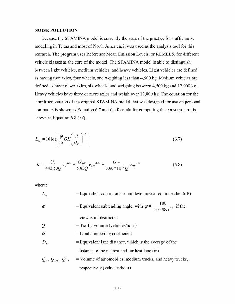
  106

NOISE POLLUTION 

  Because the STAMINA model is currently the state of the practice for traffic noise 

modeling in Texas and most of North America, it was used as the analysis tool for this 

research. The program uses Reference Mean Emission Levels, or REMELS, for different 

vehicle classes as the core of the model. The STAMINA model is able to distinguish 

between light vehicles, medium vehicles, and heavy vehicles. Light vehicles are defined 

as having two axles, four wheels, and weighing less than 4,500 kg. Medium vehicles are 

defined as having two axles, six wheels, and weighing between 4,500 kg and 12,000 kg. 

Heavy vehicles have three or more axles and weigh over 12,000 kg. The equation for the 

simplified version of the original STAMINA model that was designed for use on personal 

computers is shown as Equation 6.7 and the formula for computing the constant term is 

shown as Equation 6.8 (84). 

 

=

+αφ

115

15log10

Eeq D

QKL             (6.7) 

 

  46.12

39.281.2

10*60.383.553.442 HTHT

MTMT

AA v

QQ

vQ

Qv

QQ

K −++=       (6.8) 

 

where: 

  eqL       = Equivalent continuous sound level measured in decibel (dB) 

  φ         = Equivalent subtending angle, with  9.058.01180

αφ

+=  if the  

             view is unobstructed 

  Q         = Traffic volume (vehicles/hour) 

  α         = Land dampening coefficient 

  ED       = Equivalent lane distance, which is the average of the 

            distance to the nearest and furthest lane (m) 

  AQ ,  MTQ ,  HTQ   = Volume of automobiles, medium trucks, and heavy trucks, 

             respectively (vehicles/hour) 

  107

  Av ,  MTv ,  HTv   = Average speed of automobiles, medium trucks, and heavy 

             trucks (kilometers/hour) 

 

  In preparing the setup for STAMINA, the alignment of the roadway, as well as the 

location of the receivers, needs to be specified with a cartesian coordinate system by 

using X, Y, and Z coordinates (97). Additional information that need to be specified for 

the model are as follows: i) hourly volume for each vehicle class on each of the segments; 

ii) average speed on each of the segments; iii) whether to model barriers; and iv) whether 

to model a soft or a hard site. The output provided by STAMINA include the mean, 

standard deviation, median, tenth percentile, and ninetieth percentile Leq values (in dB), 

for all the receivers. 

  It may be noticed in Equation 6.8 that the STAMINA model is developed to make use 

of mean traffic characteristics to compute noise pollution at the link level. The model can, 

therefore, not be used to compute noise pollution at the level of the individual commuter. 

It is also not very suitable for computing noise pollution at short time increments or very 

short segment lengths. 

  By dividing the corridor into segments of reasonable length, the effect of spatial 

disaggregation, however, could be tested. With the highest level of spatial aggregation, 

the whole corridor was considered as one segment. A more disaggregate level considerd 

the AVI links as segments, whereas the most disaggregate form of spatial disaggregation 

considered the interchange links as segments. In each case the coordinates of the 

receivers were specified such that the X-coordinates correspond to the center of the 

segment under investigation, the Y-coordinates correspond to a 100-ft offset from the 

roadway, and the Z-coordinates correspond to a 5-ft elevation to simulate the height of an 

average human. 

  For illustration purposes, Figure 6.2 shows the results of the most aggregate scenario, 

as well as the most disaggregate scenario. It may be noticed in Figure 6.2 that noise 

pollution on the interchange links shows moderate changes over the lengths of the 

corridors, with the I-10 corridor showing greater variation in noise pollution than the US-

290 corridor. The mean noise pollution for the US-290 corridor at 76.8 dB is greater, 

however, than that for the I-10 corridor at 73.7 dB. A methodology that considers spatial 

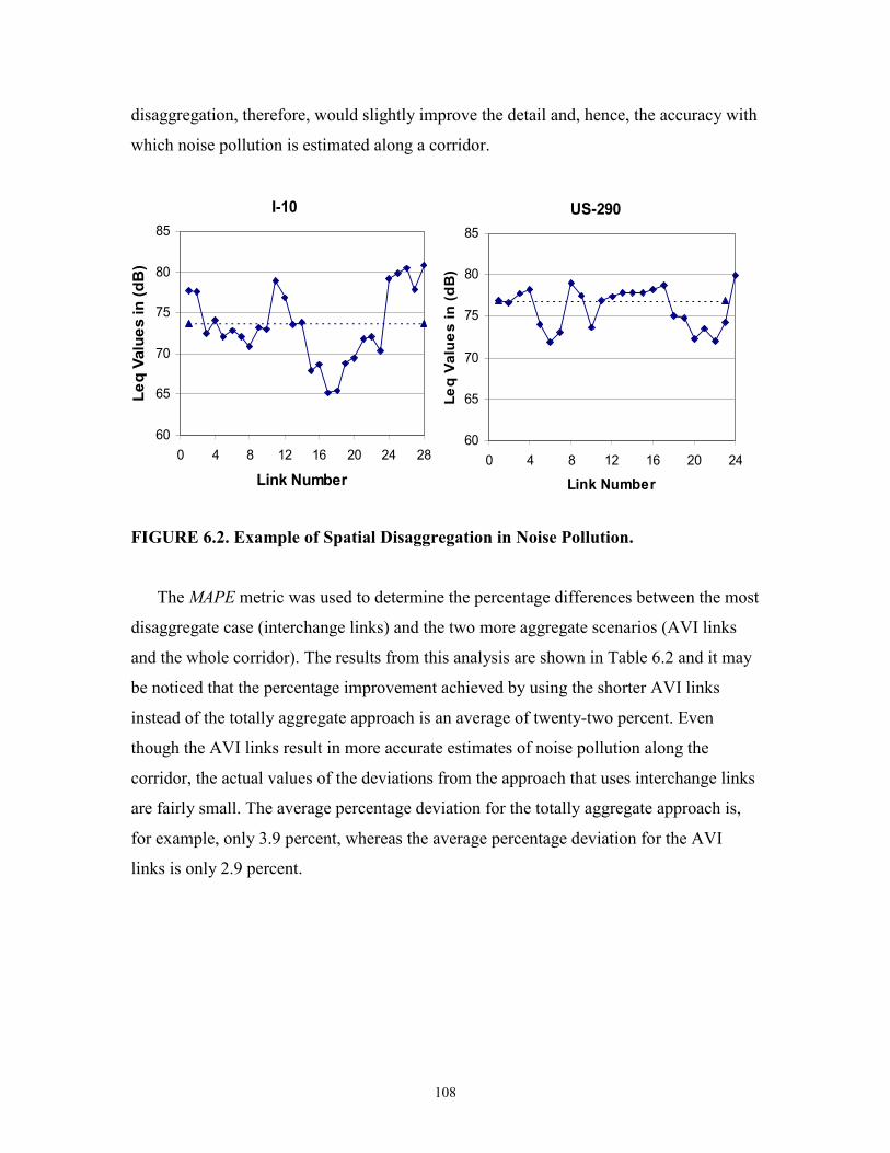
  108

disaggregation, therefore, would slightly improve the detail and, hence, the accuracy with 

which noise pollution is estimated along a corridor. 

 

 

 

 

 

 

 

 

 

 

 

 

FIGURE 6.2. Example of Spatial Disaggregation in Noise Pollution. 

 

  The MAPE metric was used to determine the percentage differences between the most 

disaggregate case (interchange links) and the two more aggregate scenarios (AVI links 

and the whole corridor). The results from this analysis are shown in Table 6.2 and it may 

be noticed that the percentage improvement achieved by using the shorter AVI links 

instead of the totally aggregate approach is an average of twenty-two percent. Even 

though the AVI links result in more accurate estimates of noise pollution along the 

corridor, the actual values of the deviations from the approach that uses interchange links 

are fairly small. The average percentage deviation for the totally aggregate approach is, 

for example, only 3.9 percent, whereas the average percentage deviation for the AVI 

links is only 2.9 percent. 

 

 

I-10

60

65

70

75

80

85

0 4 8 12 16 20 24 28

Link Number

Leq Values in (dB)

US-290

60

65

70

75

80

85

0 4 8 12 16 20 24

Link Number

Leq Values

 in (dB)

  109

TABLE 6.2  MAPE Between the Interchange Links and the Two More Aggregate 

        Scenarios 

 

Corridor  Aggregate Approach  AVI links  % Improvement 

I-10  4.9  3.4  31.0 

US-290  2.8  2.4  13.1 

Mean  3.8  2.9  22.1   

FUEL CONSUMPTION 

  There are numerous models that can be used to determine fuel consumption along a 

freeway corridor. For this research the authors decided to use the fuel consumption model 

that was developed for the macroscopic simulation model (FREFLO). This model was 

selected because of its close resemblance with the widely used energy-based model 

developed by the Australian Road Research Board (ARFCO) and the fact that it was 

validated on a Texas freeway, namely a section of I-35 near Austin (98). It may be seen 

in Equation 6.9 that the form of the model shows a nonlinear relationship with speed and 

acceleration as the two independent variables. 

 

  02

542

32

1 )( >++++=eaeex aPaPvP

vPPF           (6.9) 

 

If the expression  eaPvPP 42

31 ++  is negative, then vPFx 2=  

Where: 

  Fx      = Fuel consumption (in 1000 gal/mile) 

    v       = Mean speed (in ft/sec) 

   ae      =  Effective acceleration (in ft/sec2) 

   P1, P3, P4  = Constants derived for rolling, air, and effective inertial resistance, 

           respectively 

   P2     = A constant related to idle fuel consumption 

   P5     = A constant related to a product of inertial energy and acceleration 

  110

 

  Calibration yielded the following values for the constants: P1 = 12.76; P2 = 700; P3 = 

0.0023; P4 = 39.21; and P5 = 0.0033. These parameters were calibrated from a database 

that was developed through a study commissioned by the Federal Highway 

Administration (FHWA). The purpose of the FHWA study was to relate fuel 

consumption and emissions to vehicle speed and acceleration. The vehicles used for the 

FHWA study were representative of sixty-four percent of the 1980 to 1992 passenger 

vehicle fleet, which included pickup trucks. Fuel consumption and emissions were 

determined for each of the vehicles under different operating conditions. The results from 

the FHWA study were tables and graphs that relate fuel consumption and emissions to 

vehicle speed and acceleration (98). 

  Due to the disaggregate base of the model proposed in Equation 6.9, it can be used to 

compute fuel consumption from speed and acceleration data of individual vehicles, on a 

second-by-second basis. As a result of the findings of Chapter 5 that disaggregate 

information can provide more accurate results, it was decided to use fuel consumption 

computed by individual vehicles on a second-by-second basis as the base case for this 

research. 

  Output from the TRANSIMS model was used to determine the total fuel consumption 

of the two test corridors during the analysis period at various levels of aggregation. The 

most aggregate scenario considered the total distance traveled, mean speed, mean 

acceleration, and mean deceleration of all the vehicles during the analysis period. With a 

more disaggregate scenario these parameters were determined for each individual vehicle 

separately. These two levels of aggregation were further refined through the inclusion of 

spatial disaggregation by dividing the corridors into interchange links. With the most 

disaggregate case, the fuel consumption of each vehicle was determined on a second-by-

second basis. This scenario was used as the base case and resulted in 6,026 and 4,852 

gallons of fuel consumed during the analysis period for the I-10 and US-290 corridors, 

respectively. 

  Figure 6.3 shows the results of the most aggregate approach (all vehicles combined) 

and the most disaggregate approach (each vehicle on a second-by-second basis) for the 

various interchange links. It may be seen in this figure that the results from the aggregate 

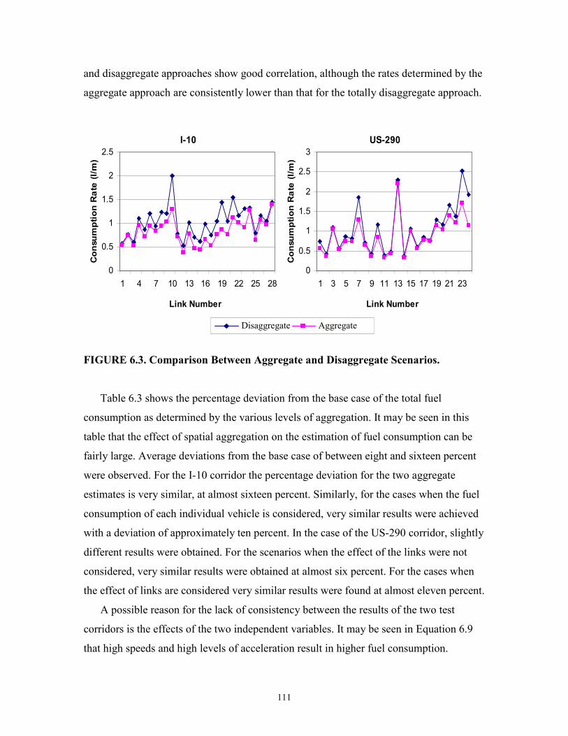
  111

and disaggregate approaches show good correlation, although the rates determined by the 

aggregate approach are consistently lower than that for the totally disaggregate approach. 

 

 

FIGURE 6.3. Comparison Between Aggregate and Disaggregate Scenarios. 

 

  Table 6.3 shows the percentage deviation from the base case of the total fuel 

consumption as determined by the various levels of aggregation. It may be seen in this 

table that the effect of spatial aggregation on the estimation of fuel consumption can be 

fairly large. Average deviations from the base case of between eight and sixteen percent 

were observed. For the I-10 corridor the percentage deviation for the two aggregate 

estimates is very similar, at almost sixteen percent. Similarly, for the cases when the fuel 

consumption of each individual vehicle is considered, very similar results were achieved 

with a deviation of approximately ten percent. In the case of the US-290 corridor, slightly 

different results were obtained. For the scenarios when the effect of the links were not 

considered, very similar results were obtained at almost six percent. For the cases when 

the effect of links are considered very similar results were found at almost eleven percent. 

  A possible reason for the lack of consistency between the results of the two test 

corridors is the effects of the two independent variables. It may be seen in Equation 6.9 

that high speeds and high levels of acceleration result in higher fuel consumption. 

US-290

0

0.5

1

1.5

2

2.5

3

1 3 5 7 9 11 13 15 17 19 21 23

Link NumberConsumption Rate (l/m)

I-10

0

0.5

1

1.5

2

2.5

1 4 7 10 13 16 19 22 25 28

Link Number

Consumption Rate (l/m)

Disaggregate  Aggregate 

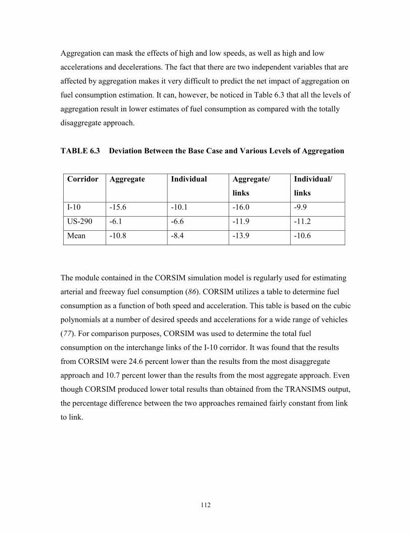
  112

Aggregation can mask the effects of high and low speeds, as well as high and low 

accelerations and decelerations. The fact that there are two independent variables that are 

affected by aggregation makes it very difficult to predict the net impact of aggregation on 

fuel consumption estimation. It can, however, be noticed in Table 6.3 that all the levels of 

aggregation result in lower estimates of fuel consumption as compared with the totally 

disaggregate approach. 

 

TABLE 6.3  Deviation Between the Base Case and Various Levels of Aggregation 

 

Corridor  Aggregate  Individual  Aggregate/ 

links 

Individual/ 

links 

I-10  -15.6  -10.1  -16.0  -9.9 

US-290  -6.1  -6.6  -11.9  -11.2 

Mean  -10.8  -8.4  -13.9  -10.6 

 

 

The module contained in the CORSIM simulation model is regularly used for estimating 

arterial and freeway fuel consumption (86). CORSIM utilizes a table to determine fuel 

consumption as a function of both speed and acceleration. This table is based on the cubic 

polynomials at a number of desired speeds and accelerations for a wide range of vehicles 

(77). For comparison purposes, CORSIM was used to determine the total fuel 

consumption on the interchange links of the I-10 corridor. It was found that the results 

from CORSIM were 24.6 percent lower than the results from the most disaggregate 

approach and 10.7 percent lower than the results from the most aggregate approach. Even 

though CORSIM produced lower total results than obtained from the TRANSIMS output, 

the percentage difference between the two approaches remained fairly constant from link 

to link. 

 

 

  113

CONCLUDING REMARKS 

  The information used as input into typical emission models traditionally has been 

obtained from macroscopic transportation planning models. Over the past ten years, 

however, there has been a definite shift to micro-simulation modeling and the use of ITS, 

providing numerous possibilities for capturing detailed transportation related information. 

These new disaggregate models and data sources provide for alternative ways of 

estimating VKT and average speed as important inputs into an emission model such as 

MOBILE 5a. 

  Two scenarios were constructed. In the case of Scenario 1, the average speed and 

total distance traveled for all vehicles in each vehicle class were determined for each 

spatial and temporal aggregation level. In the case of Scenario 2, the average speed and 

distance traveled of each individual vehicle within each vehicle class were determined for 

each spatial and temporal aggregation level. In order to have a fixed reference point, the 

current state of the practice, namely Scenario 1 applied at the base link level, was used as 

the base case. 

  It was found that all the deviations from the base case are positive, indicating that the 

most aggregate scenario (base case) results in lower emissions than results obtained with 

the various levels of spatial and temporal disaggregation. It also was found that for this 

test corridor larger emission estimates could be obtained if Scenario 2 was used, as 

opposed to Scenario 1. Therefore, if the hypothesis is true that Scenario 2 is more 

accurate than Scenario 1, the total emissions for the test corridor is higher than what is 

estimated through the conventional approach. 

  TRANSIMS was used to simulate output from loop detectors, AVI technology, and 

AVL technology. It was found that the total emissions calculated with loop detector data 

were slightly higher than that obtained with the base case. The reason for this is that in 

the case of loop detector data the speeds are based on time mean speed and for the base 

case they are based on space mean speed. Total emissions calculated with AVI and AVL 

technology were very similar and considerably higher than that obtained with the base 

case. It is hypothesized that the reason for this is that a large percentage of high emitting 

low speeds are not accounted for with the conventional aggregate approach. 

  114

  To illustrate that the results are not related to the type of model used, the analyses 

were repeated using CORSIM, and comparable aggregation effects were obtained. 

Additionally, the analysis was repeated in another study, using the emissions module 

within the EMPRO model and the differences in emission estimation were found to be 

comparable with the results of this study. This shows that aggregation can have an 

important effect on emission estimation, regardless of the type of simulation or emissions 

model used. 

  It was shown in this study that the level of aggregation of the input data can have an 

important effect on the final results. Because emission modeling has a direct bearing on 

whether an area is considered to be in attainment or not, it is very important to ensure that 

these models are applied in an accurate and consistent way. The shift to micro-simulation 

modeling and ITS has created opportunities to use speed and VKT information at 

disaggregate levels. There is, therefore, a need to: i) develop emissions models that can 

perform adequately at these disaggregate levels, and ii) provide policy guidelines to 

ensure consistency of applications. 

  With regard to noise pollution, the STAMINA model was used to quantify noise 

pollution along the corridors at various levels of spatial disaggregation. It was found that 

a twenty-two percent improvement could be achieved by using the shorter AVI links 

instead of the totally aggregate corridor level as compared with the approach that uses 

interchange links. The actual values of the deviations from the approach that uses 

interchange links, however, are fairly small, with differences of only 3.9 percent if the 

whole corridor is used and 2.9 percent if AVI links are used. 

  In the case of fuel consumption the effect of spatial aggregation can be fairly large. 

Average deviations from the totally disaggregate case (calculated for each vehicle on a 

second-by-second basis) of between six and sixteen percent were observed. It was found 

that incorporating the effect of the individual vehicles provides slightly better results. For 

comparison purposes, CORSIM was used to determine the total fuel consumption on the 

interchange links of the I-10 corridor. It was found that even though CORSIM produced 

results that were between ten and twenty-five percent lower than the results obtained 

from the TRANSIMS output, the percentage difference between the two approaches 

remained fairly constant from link to link. 

  115

  The following chapter illustrates a number of applications with performance measures 

of sustainable transportation, namely: i) to use the quantified performance measures in 

the decision-making process; ii) to use equivalency factors for allocating responsibility 

for vehicular emission; and iii) to propose and use a sustainable transportation index to 

determine the sustainability of an existing or planned project. 

 

 

 

 

 

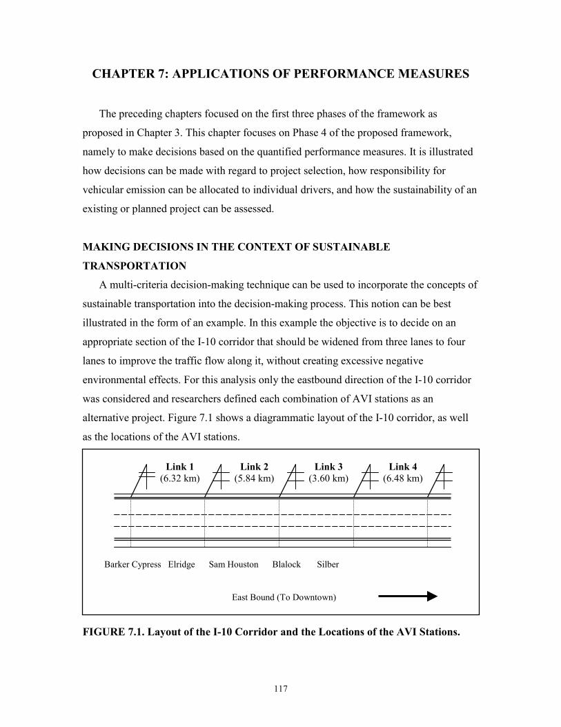
117 

CHAPTER 7: APPLICATIONS OF PERFORMANCE MEASURES  

  The preceding chapters focused on the first three phases of the framework as 

proposed in Chapter 3. This chapter focuses on Phase 4 of the proposed framework, 

namely to make decisions based on the quantified performance measures. It is illustrated 

how decisions can be made with regard to project selection, how responsibility for 

vehicular emission can be allocated to individual drivers, and how the sustainability of an 

existing or planned project can be assessed. 

 

MAKING DECISIONS IN THE CONTEXT OF SUSTAINABLE 

TRANSPORTATION 

  A multi-criteria decision-making technique can be used to incorporate the concepts of 

sustainable transportation into the decision-making process. This notion can be best 

illustrated in the form of an example. In this example the objective is to decide on an 

appropriate section of the I-10 corridor that should be widened from three lanes to four 

lanes to improve the traffic flow along it, without creating excessive negative 

environmental effects. For this analysis only the eastbound direction of the I-10 corridor 

was considered and researchers defined each combination of AVI stations as an 

alternative project. Figure 7.1 shows a diagrammatic layout of the I-10 corridor, as well 

as the locations of the AVI stations. 

 FIGURE 7.1. Layout of the I-10 Corridor and the Locations of the AVI Stations.  

Link 1 (6.32 km) 

East Bound (To Downtown) 

Link 2 (5.84 km) 

Link 3 (3.60 km) 

Link 4 (6.48 km) 

Barker Cypress   Elridge      Sam Houston      Blalock       Silber 

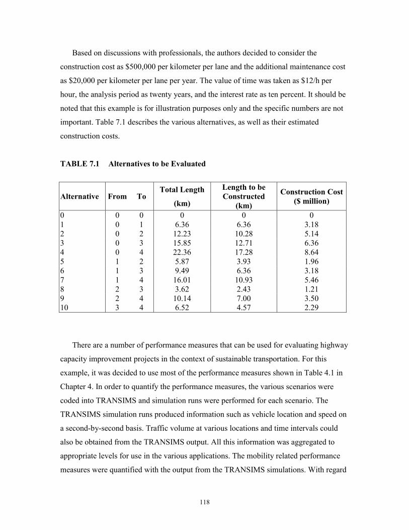
  118

  Based on discussions with professionals, the authors decided to consider the 

construction cost as $500,000 per kilometer per lane and the additional maintenance cost 

as $20,000 per kilometer per lane per year. The value of time was taken as $12/h per 

hour, the analysis period as twenty years, and the interest rate as ten percent. It should be 

noted that this example is for illustration purposes only and the specific numbers are not 

important. Table 7.1 describes the various alternatives, as well as their estimated 

construction costs. 

 

TABLE 7.1  Alternatives to be Evaluated  

Alternative  From  To Total Length 

(km) 

Length to be Constructed 

(km) 

Construction Cost($ million) 

0  0  0  0  0  0 1  0  1  6.36  6.36  3.18 2  0  2  12.23  10.28  5.14 3  0  3  15.85  12.71  6.36 4  0  4  22.36  17.28  8.64 5  1  2  5.87  3.93  1.96 6  1  3  9.49  6.36  3.18 7  1  4  16.01  10.93  5.46 8  2  3  3.62  2.43  1.21 9  2  4  10.14  7.00  3.50 10  3  4  6.52  4.57  2.29  

 

  There are a number of performance measures that can be used for evaluating highway 

capacity improvement projects in the context of sustainable transportation. For this 

example, it was decided to use most of the performance measures shown in Table 4.1 in 

Chapter 4. In order to quantify the performance measures, the various scenarios were 

coded into TRANSIMS and simulation runs were performed for each scenario. The 

TRANSIMS simulation runs produced information such as vehicle location and speed on 

a second-by-second basis. Traffic volume at various locations and time intervals could 

also be obtained from the TRANSIMS output. All this information was aggregated to 

appropriate levels for use in the various applications. The mobility related performance 

measures were quantified with the output from the TRANSIMS simulations. With regard 

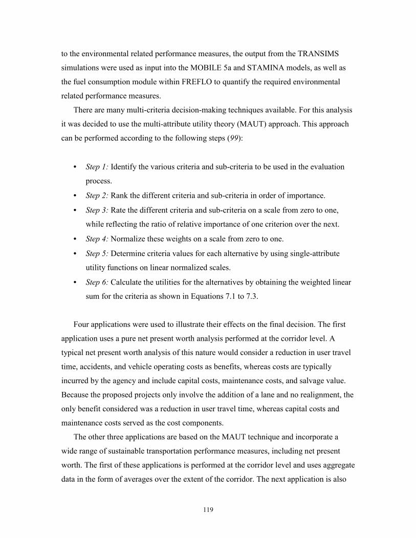
  119

to the environmental related performance measures, the output from the TRANSIMS 

simulations were used as input into the MOBILE 5a and STAMINA models, as well as 

the fuel consumption module within FREFLO to quantify the required environmental 

related performance measures. 

  There are many multi-criteria decision-making techniques available. For this analysis 

it was decided to use the multi-attribute utility theory (MAUT) approach. This approach 

can be performed according to the following steps (99): 

 

• Step 1: Identify the various criteria and sub-criteria to be used in the evaluation 

process. 

• Step 2: Rank the different criteria and sub-criteria in order of importance.  

• Step 3: Rate the different criteria and sub-criteria on a scale from zero to one, 

while reflecting the ratio of relative importance of one criterion over the next. 

• Step 4: Normalize these weights on a scale from zero to one.  

• Step 5: Determine criteria values for each alternative by using single-attribute 

utility functions on linear normalized scales.  

• Step 6: Calculate the utilities for the alternatives by obtaining the weighted linear 

sum for the criteria as shown in Equations 7.1 to 7.3. 

 

  Four applications were used to illustrate their effects on the final decision. The first 

application uses a pure net present worth analysis performed at the corridor level. A 

typical net present worth analysis of this nature would consider a reduction in user travel 

time, accidents, and vehicle operating costs as benefits, whereas costs are typically 

incurred by the agency and include capital costs, maintenance costs, and salvage value. 

Because the proposed projects only involve the addition of a lane and no realignment, the 

only benefit considered was a reduction in user travel time, whereas capital costs and 

maintenance costs served as the cost components. 

  The other three applications are based on the MAUT technique and incorporate a 

wide range of sustainable transportation performance measures, including net present 

worth. The first of these applications is performed at the corridor level and uses aggregate 

data in the form of averages over the extent of the corridor. The next application is also 

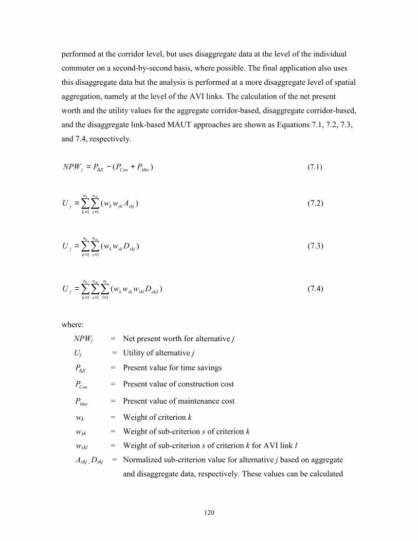
  120

performed at the corridor level, but uses disaggregate data at the level of the individual 

commuter on a second-by-second basis, where possible. The final application also uses 

this disaggregate data but the analysis is performed at a more disaggregate level of spatial 

aggregation, namely at the level of the AVI links. The calculation of the net present 

worth and the utility values for the aggregate corridor-based, disaggregate corridor-based, 

and the disaggregate link-based MAUT approaches are shown as Equations 7.1, 7.2, 7.3, 

and 7.4, respectively.  

)( MntConXj PPPNPW +−= ∆               (7.1) 

 

)(1 1∑∑

= =

=k skn

k

n

sskjskkj AwwU               (7.2) 

 

)(1 1∑∑

= =

=k skn

k

n

sskjskkj DwwU               (7.3) 

 

)(1 1 1∑∑∑

= = =

=k sk ln

k

n

s

n

lskjlsklskkj DwwwU             (7.4) 

               

where: 

  NPWj    =  Net present worth for alternative j 

  Uj       =  Utility of alternative j 

  XP∆     =  Present value for time savings 

  ConP     =  Present value of construction cost 

  MntP     =  Present value of maintenance cost 

   wk      =  Weight of criterion k 

   wsk     =  Weight of sub-criterion s of criterion k 

   wskl    =  Weight of sub-criterion s of criterion k for AVI link l 

   Askj , Dskj   =  Normalized sub-criterion value for alternative j based on aggregate 

          and disaggregate data, respectively. These values can be calculated 

  121

          as follows:  )(, skjskskjskj sfDA =  

  Askjl , Dskjl  =  Normalized sub-criterion value for alternative j on AVI link l based  

          on aggregate and disaggregate data, respectively. These values can 

          be calculated as follows:  )(, skjlskskjlskjl sfDA =  

  sskj      =  Value of sub-criterion s of criterion k for alternative j 

   sskjl    =  Value of sub-criterion s of criterion k for alternative j on AVI link l 

  )(xf sk    =  Single-attribute utility function on a normalized scale from 0 to 1 

          for sub-criterion s of criterion k 

 

  The criteria weights were determined by applying professional judgment and 

following steps 1 to 4 as discussed above. These weights are shown in Table 7.2. It is 

possible to allocate weights to the various sub-criteria within each of the AVI links, as 

illustrated in Equation 7.4. This option allows the decision-maker to allocate importance 

to certain links in terms of certain criteria. The CBD and surrounding areas of a city 

might, for example, be experiencing high levels of air pollution. The decision-maker 

would, therefore, allocate heavier weights for vehicular emission to links that are in the 

area of high air pollution. For illustration purposes, it was decided to allocate more 

importance to the AVI links closer to the CBD. Weights of nine, eighteen, twenty-seven, 

and forty-eight percent were allocated to all the criteria within the AVI links, from the 

furthest AVI link to the one that is closest to the CBD. 

  

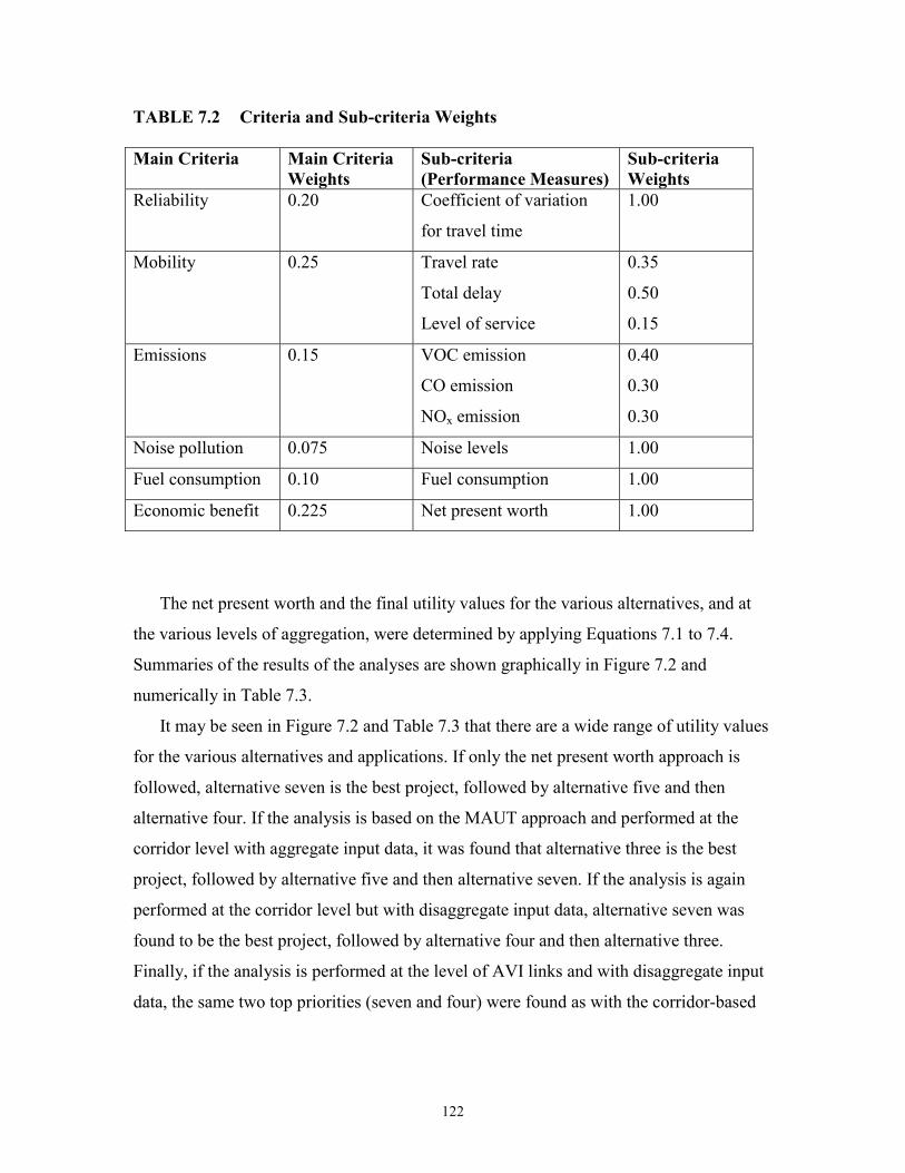
  122

TABLE 7.2  Criteria and Sub-criteria Weights  Main Criteria  Main Criteria 

Weights Sub-criteria (Performance Measures) 

Sub-criteria Weights 

Reliability  0.20  Coefficient of variation 

for travel time 

1.00 

Mobility 

 

0.25  Travel rate 

Total delay 

Level of service 

0.35 

0.50 

0.15 

Emissions 

 

0.15  VOC emission 

CO emission 

NOx emission 

0.40 

0.30 

0.30 

Noise pollution  0.075  Noise levels  1.00 

Fuel consumption  0.10  Fuel consumption  1.00 

Economic benefit  0.225  Net present worth  1.00 

 

 

  The net present worth and the final utility values for the various alternatives, and at 

the various levels of aggregation, were determined by applying Equations 7.1 to 7.4. 

Summaries of the results of the analyses are shown graphically in Figure 7.2 and 

numerically in Table 7.3. 

  It may be seen in Figure 7.2 and Table 7.3 that there are a wide range of utility values 

for the various alternatives and applications. If only the net present worth approach is 

followed, alternative seven is the best project, followed by alternative five and then 

alternative four. If the analysis is based on the MAUT approach and performed at the 

corridor level with aggregate input data, it was found that alternative three is the best 

project, followed by alternative five and then alternative seven. If the analysis is again 

performed at the corridor level but with disaggregate input data, alternative seven was 

found to be the best project, followed by alternative four and then alternative three. 

Finally, if the analysis is performed at the level of AVI links and with disaggregate input 

data, the same two top priorities (seven and four) were found as with the corridor-based  

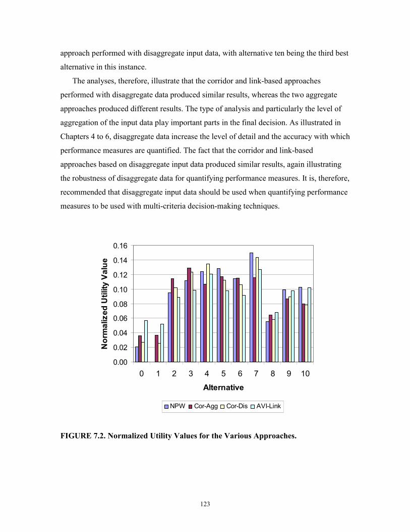
  123

approach performed with disaggregate input data, with alternative ten being the third best 

alternative in this instance. 

  The analyses, therefore, illustrate that the corridor and link-based approaches 

performed with disaggregate data produced similar results, whereas the two aggregate 

approaches produced different results. The type of analysis and particularly the level of 

aggregation of the input data play important parts in the final decision. As illustrated in 

Chapters 4 to 6, disaggregate data increase the level of detail and the accuracy with which 

performance measures are quantified. The fact that the corridor and link-based 

approaches based on disaggregate input data produced similar results, again illustrating 

the robustness of disaggregate data for quantifying performance measures. It is, therefore, 

recommended that disaggregate input data should be used when quantifying performance 

measures to be used with multi-criteria decision-making techniques. 

 

 

FIGURE 7.2. Normalized Utility Values for the Various Approaches. 

 

 

0.00

0.02

0.04

0.06

0.08

0.10

0.12

0.14

0.16

0 1 2 3 4 5 6 7 8 9 10

Alternative

Normalized

 Utility Value

NPW Cor-Agg Cor-Dis AVI-Link

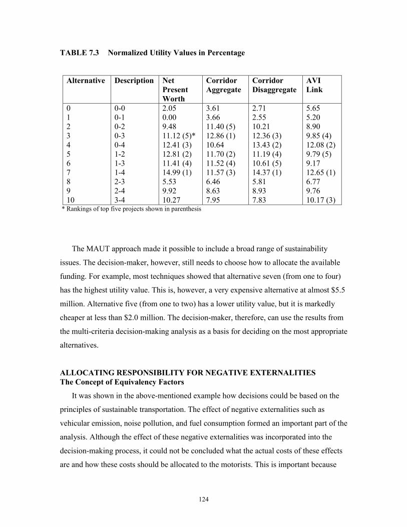
  124

TABLE 7.3  Normalized Utility Values in Percentage 

 

Alternative  Description  Net Present Worth 

Corridor Aggregate 

Corridor Disaggregate 

AVI Link 

0  0-0  2.05  3.61  2.71  5.65 1  0-1  0.00  3.66  2.55  5.20 2  0-2  9.48  11.40 (5)  10.21  8.90 3  0-3  11.12 (5)*  12.86 (1)  12.36 (3)  9.85 (4) 4  0-4  12.41 (3)  10.64  13.43 (2)  12.08 (2) 5  1-2  12.81 (2)  11.70 (2)  11.19 (4)  9.79 (5) 6  1-3  11.41 (4)  11.52 (4)  10.61 (5)  9.17 7  1-4  14.99 (1)  11.57 (3)  14.37 (1)  12.65 (1) 8  2-3  5.53  6.46  5.81  6.77 9  2-4  9.92  8.63  8.93  9.76 10  3-4  10.27  7.95  7.83  10.17 (3) 

 * Rankings of top five projects shown in parenthesis  

 

 

  The MAUT approach made it possible to include a broad range of sustainability 

issues. The decision-maker, however, still needs to choose how to allocate the available 

funding. For example, most techniques showed that alternative seven (from one to four) 

has the highest utility value. This is, however, a very expensive alternative at almost $5.5 

million. Alternative five (from one to two) has a lower utility value, but it is markedly 

cheaper at less than $2.0 million. The decision-maker, therefore, can use the results from 

the multi-criteria decision-making analysis as a basis for deciding on the most appropriate 

alternatives. 

 

ALLOCATING RESPONSIBILITY FOR NEGATIVE EXTERNALITIES The Concept of Equivalency Factors 

  It was shown in the above-mentioned example how decisions could be based on the 

principles of sustainable transportation. The effect of negative externalities such as 

vehicular emission, noise pollution, and fuel consumption formed an important part of the 

analysis. Although the effect of these negative externalities was incorporated into the 

decision-making process, it could not be concluded what the actual costs of these effects 

are and how these costs should be allocated to the motorists. This is important because 

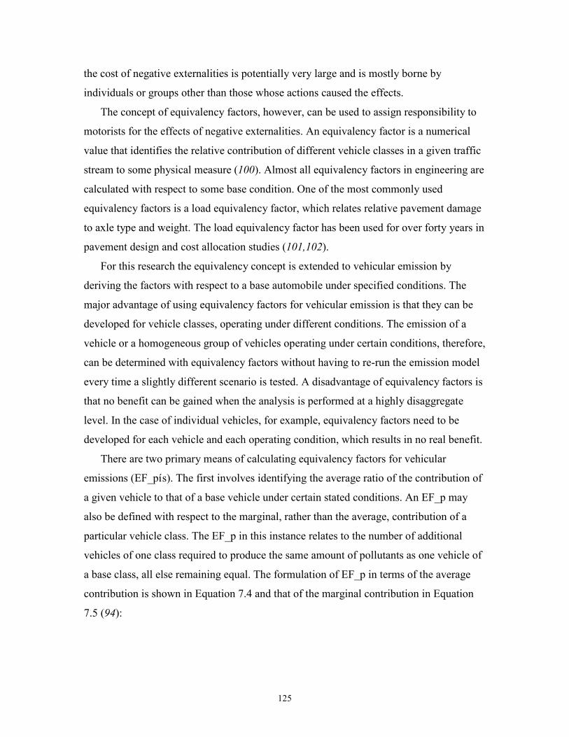
  125

the cost of negative externalities is potentially very large and is mostly borne by 

individuals or groups other than those whose actions caused the effects. 

  The concept of equivalency factors, however, can be used to assign responsibility to 

motorists for the effects of negative externalities. An equivalency factor is a numerical 

value that identifies the relative contribution of different vehicle classes in a given traffic 

stream to some physical measure (100). Almost all equivalency factors in engineering are 

calculated with respect to some base condition. One of the most commonly used 

equivalency factors is a load equivalency factor, which relates relative pavement damage 

to axle type and weight. The load equivalency factor has been used for over forty years in 

pavement design and cost allocation studies (101,102). 

  For this research the equivalency concept is extended to vehicular emission by 

deriving the factors with respect to a base automobile under specified conditions. The 

major advantage of using equivalency factors for vehicular emission is that they can be 

developed for vehicle classes, operating under different conditions. The emission of a 

vehicle or a homogeneous group of vehicles operating under certain conditions, therefore, 

can be determined with equivalency factors without having to re-run the emission model 

every time a slightly different scenario is tested. A disadvantage of equivalency factors is 

that no benefit can be gained when the analysis is performed at a highly disaggregate 

level. In the case of individual vehicles, for example, equivalency factors need to be 

developed for each vehicle and each operating condition, which results in no real benefit. 

  There are two primary means of calculating equivalency factors for vehicular 

emissions (EF_pís). The first involves identifying the average ratio of the contribution of 

a given vehicle to that of a base vehicle under certain stated conditions. An EF_p may 

also be defined with respect to the marginal, rather than the average, contribution of a 

particular vehicle class. The EF_p in this instance relates to the number of additional 

vehicles of one class required to produce the same amount of pollutants as one vehicle of 

a base class, all else remaining equal. The formulation of EF_p in terms of the average 

contribution is shown in Equation 7.4 and that of the marginal contribution in Equation 

7.5 (94): 

 

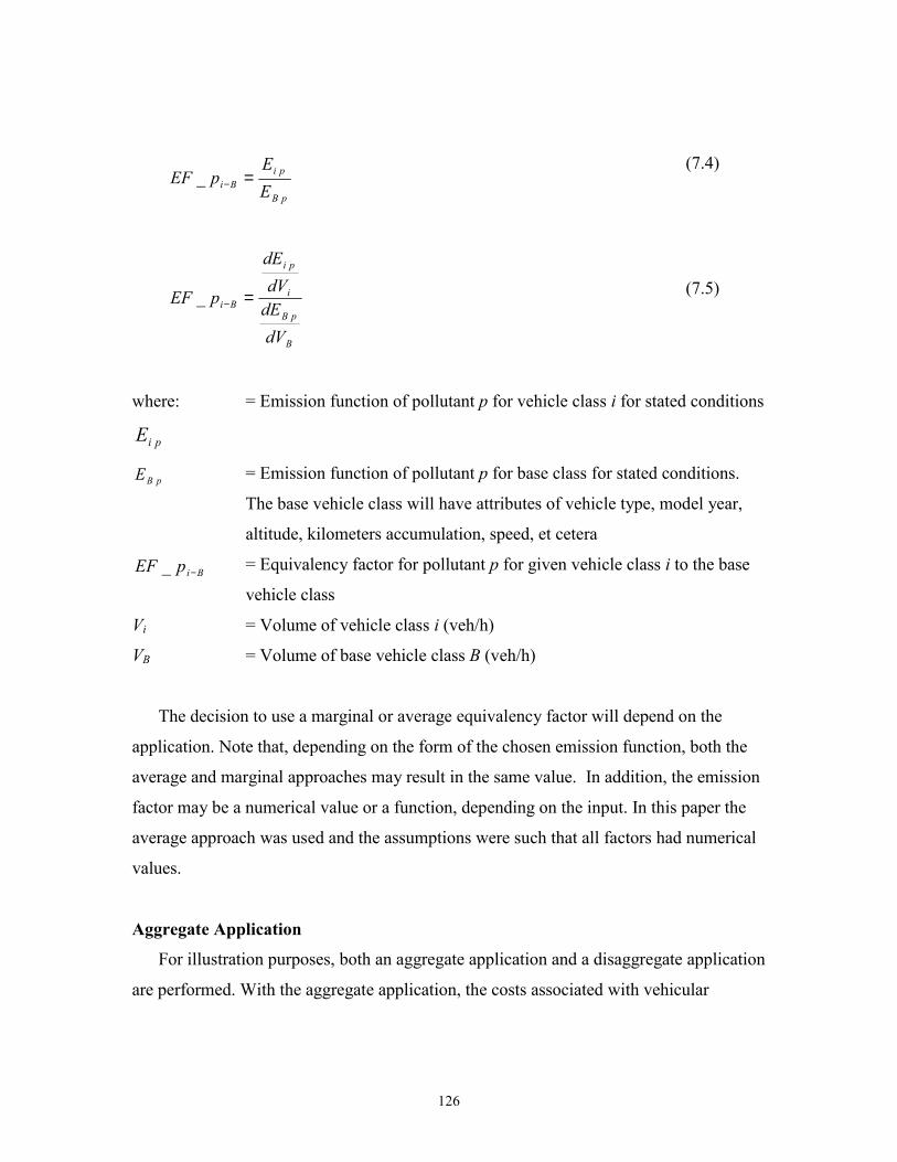
  126

  

        pB

piBi E

EpEF

 

 _ =−  

 

 (7.4) 

 

 

        

B

pB

i

pi

Bi

dVdEdVdE

pEF 

 

_ =−  

 

 

 

 (7.5) 

where: 

piE    

= Emission function of pollutant p for vehicle class i for stated conditions 

pBE     = Emission function of pollutant p for base class for stated conditions. 

The base vehicle class will have attributes of vehicle type, model year, 

altitude, kilometers accumulation, speed, et cetera 

BipEF −_   = Equivalency factor for pollutant p for given vehicle class i to the base 

vehicle class  

Vi  = Volume of vehicle class i (veh/h) 

VB  = Volume of base vehicle class B (veh/h) 

 

  The decision to use a marginal or average equivalency factor will depend on the 

application. Note that, depending on the form of the chosen emission function, both the 

average and marginal approaches may result in the same value.  In addition, the emission 

factor may be a numerical value or a function, depending on the input. In this paper the 

average approach was used and the assumptions were such that all factors had numerical 

values. 

 

Aggregate Application 

  For illustration purposes, both an aggregate application and a disaggregate application 

are performed. With the aggregate application, the costs associated with vehicular 

  127

emissions are determined for the eight vehicle classes, whereas with the disaggregate 

application the costs are determined for individual vehicles. 

  A base vehicle can be selected from any vehicle class, model year, and speed, 

provided this combination is contained in the MOBILE 5a model. For this research the 

base vehicle was taken as a standard LDGV from the 2007 vehicle model year that is 

travelling at a speed of 32 km/h (average speed of the Federal Test Procedure cycle). The 

MOBILE 5a model yielded emission rates of 0.0766, 0.2233, and 0.0674 g/km for VOC, 

CO, and NOx pollution, respectively, for the base vehicle at the selected speed and study 

area characteristics. 

  The TRANSIMS model was used to perform simulation runs for the corridor during 

the peak hour. Individual vehicles of the TRANSIMS output were randomly allocated to 

the eight vehicle classes based on the VMT mix of these classes. For this analysis the 

VMT mix was obtained from work performed by the Texas Transportation Institute to 

develop gridded mobile source emissions for the Houston-Galveston nonattainment 

counties. It was estimated using the Texas Department of Transportation (TxDOT) 

weekday vehicle classification data. The TxDOT classification counts allocate vehicles 

into the standard FHWA vehicle classifications. These categories were then converted 

into the eight EPA vehicle classes by using various conversion functions. 

  Volume and speed data were obtained for the eight vehicle classes using the 

TRANSIMS output. This information could be used as input into the MOBILE 5a model 

to yield emission rates for the eight vehicle classes and for each of the three pollutant 

types analyzed. By applying Equation 7.4 these emission rates, along with the emission 

rates for the base case, could be used to produce the required equivalency factors. The 

results of this analysis are included in Table 7.4. It may be seen in this table, for example, 

that the emission rate for VOC pollution for Class 1 vehicles traveling at a speed of 76 

km/h is 0.58 g/km. The emission rate for VOC pollution of the base vehicle is 0.0766 

g/km. The equivalency factor for Class 1 vehicles traveling at 76 km/h is, therefore, 0.58 

divided by 0.0766, which is 7.6 as shown in Table 7.4. 

 

 

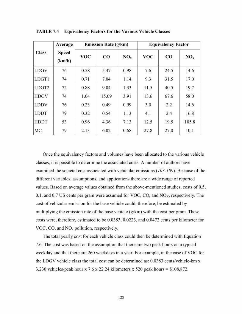
  128

TABLE 7.4  Equivalency Factors for the Various Vehicle Classes  

Emission Rate (g/km)  Equivalency Factor 

Class 

Average 

Speed 

(km/h) VOC  CO  NOx  VOC  CO  NOx 

LDGV  76  0.58  5.47  0.98  7.6  24.5  14.6 

LDGT1  74  0.71  7.04  1.14  9.3  31.5  17.0 

LDGT2  72  0.88  9.04  1.33  11.5  40.5  19.7 

HDGV  74  1.04  15.09  3.91  13.6  67.6  58.0 

LDDV  76  0.23  0.49  0.99  3.0  2.2  14.6 

LDDT  79  0.32  0.54  1.13  4.1  2.4  16.8 

HDDT  53  0.96  4.36  7.13  12.5  19.5  105.8 

MC  79  2.13  6.02  0.68  27.8  27.0  10.1  

 

  Once the equivalency factors and volumes have been allocated to the various vehicle 

classes, it is possible to determine the associated costs. A number of authors have 

examined the societal cost associated with vehicular emissions (103-109). Because of the 

different variables, assumptions, and applications there are a wide range of reported 

values. Based on average values obtained from the above-mentioned studies, costs of 0.5, 

0.1, and 0.7 US cents per gram were assumed for VOC, CO, and NOX, respectively. The 

cost of vehicular emission for the base vehicle could, therefore, be estimated by 

multiplying the emission rate of the base vehicle (g/km) with the cost per gram. These 

costs were, therefore, estimated to be 0.0383, 0.0223, and 0.0472 cents per kilometer for 

VOC, CO, and NOx pollution, respectively. 

  The total yearly cost for each vehicle class could then be determined with Equation 

7.6. The cost was based on the assumption that there are two peak hours on a typical 

weekday and that there are 260 weekdays in a year. For example, in the case of VOC for 

the LDGV vehicle class the total cost can be determined as: 0.0383 cents/vehicle-km x 

3,230 vehicles/peak hour x 7.6 x 22.24 kilometers x 520 peak hours = $108,872. 

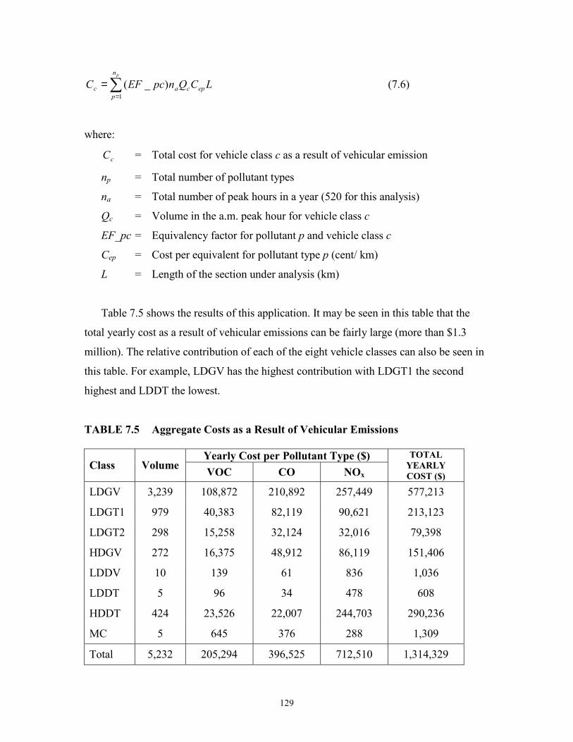
  129

∑=

=pn

pepcac LCQnpcEFC

1

)_(             (7.6) 

 

where: 

  cC    =  Total cost for vehicle class c as a result of vehicular emission 

  np    =  Total number of pollutant types 

  na    =  Total number of peak hours in a year (520 for this analysis) 

  Qc    =  Volume in the a.m. peak hour for vehicle class c 

  EF_pc =  Equivalency factor for pollutant p and vehicle class c 

  Cep   =  Cost per equivalent for pollutant type p (cent/ km) 

  L    =  Length of the section under analysis (km) 

 

  Table 7.5 shows the results of this application. It may be seen in this table that the 

total yearly cost as a result of vehicular emissions can be fairly large (more than $1.3 

million). The relative contribution of each of the eight vehicle classes can also be seen in 

this table. For example, LDGV has the highest contribution with LDGT1 the second 

highest and LDDT the lowest. 

 

TABLE 7.5  Aggregate Costs as a Result of Vehicular Emissions  

Yearly Cost per Pollutant Type ($) Class  Volume  VOC  CO  NOx 

TOTAL YEARLY COST ($) 

LDGV  3,239  108,872  210,892  257,449  577,213 

LDGT1  979  40,383  82,119  90,621  213,123 

LDGT2  298  15,258  32,124  32,016  79,398 

HDGV  272  16,375  48,912  86,119  151,406 

LDDV  10  139  61  836  1,036 

LDDT  5  96  34  478  608 

HDDT  424  23,526  22,007  244,703  290,236 

MC  5  645  376  288  1,309 

Total  5,232  205,294  396,525  712,510  1,314,329 

  130

Disaggregate Application 

  Data collection techniques such as AVI and micro-simulation models such as 

TRANSIMS make it possible to keep track of individual vehicles over space and time. 

This ability allows the planner to determine equivalency factors at a disaggregate or 

individual vehicle level. For this analysis, equivalency factors were used to determine the 

emissions cost associated with commuters. 

  The concept is illustrated by using the observed AVI data that were obtained for the I-

10 corridor. The mean speeds and number of trips undertaken by individual vehicles 

could be determined with the AVI data. For illustration purposes, three randomly selected 

regular commuters were chosen for this analysis. 

  To illustrate the effect of equivalency factors, vehicle one was considered as a light 

passenger car (LDGV), vehicle two as a light-duty gasoline fueled truck with a gross 

weight between 6,000 and 8,500 pounds (LDGT2), and vehicle three as a heavy-duty 

diesel truck with a gross weight over 8,500 pounds (HDDT). In addition, vehicle one was 

assumed to be a 2000 model year, whereas vehicles two and three were assumed to be 

1995 and 1990 model year vehicles, respectively. October 19, 1996, was selected as 

analysis day because on that day all three vehicles made trips along the full extent of the 

corridor and were detected at each of the five AVI stations. 

  MOBILE 5a was again used to produce the required emission rates for the various 

vehicle classes, model years, and speeds. Equivalency factors, therefore, could be 

determined for each vehicle, on each of the AVI links, and for each pollutant type. The 

costs as a result of vehicular emissions for the three test vehicles could be determined by 

multiplying the equivalency factor with the cost per equivalent and the length of the AVI 

link, as shown in Equation 7.7. 

 

∑∑∑= = =

=k l pn

k

n

ll

n

plepj LCpjdlEFC

1 1

)_(             (7.7) 

 

where: 

  jC      =  Total cost for vehicle j during the month under analysis 

  np      =  Total number of pollutant types 

  131

  nl      =  Total number of AVI links in the corridor 

  nk      =  Total number of times that vehicle j is detected on the AVI links 

  EF_pjdl  =  Equivalency factor for pollutant p, vehicle j, trip d and AVI link l 

  Cep     =  Cost per equivalent for pollutant type p (cent/ km) 

  Ll      =  Length of AVI link l (km) 

 

  For example, MOBILE 5a yielded a VOC emission rate of 0.1226 g/km for vehicle 

one traveling at an average speed of 100.9 km/h along AVI link one. Therefore, 0.1226 

divided by the VOC emission rate of the base vehicle (0.0766) yields an equivalency 

factor of 1.6. The cost as a result of VOC emission on AVI link one can be determined 

as: 1.6 x 0.0383 cents per kilometer x 6.32 kilometers = 0.387 cents. Similarly, the cost 

can be determined for all the other pollutants, AVI links, and vehicles. 

  The results of this analysis are included in Table 7.6. It may be seen in this table that 

the cost imposed by each vehicle, as a result of air pollution, can be determined for each 

AVI link. It may also be seen that the costs range from 1 cent to almost 60 cents, 

depending on the length of the AVI link, vehicle class, age of the vehicle, and the mean 

speed of the vehicle on the link. 

 

 

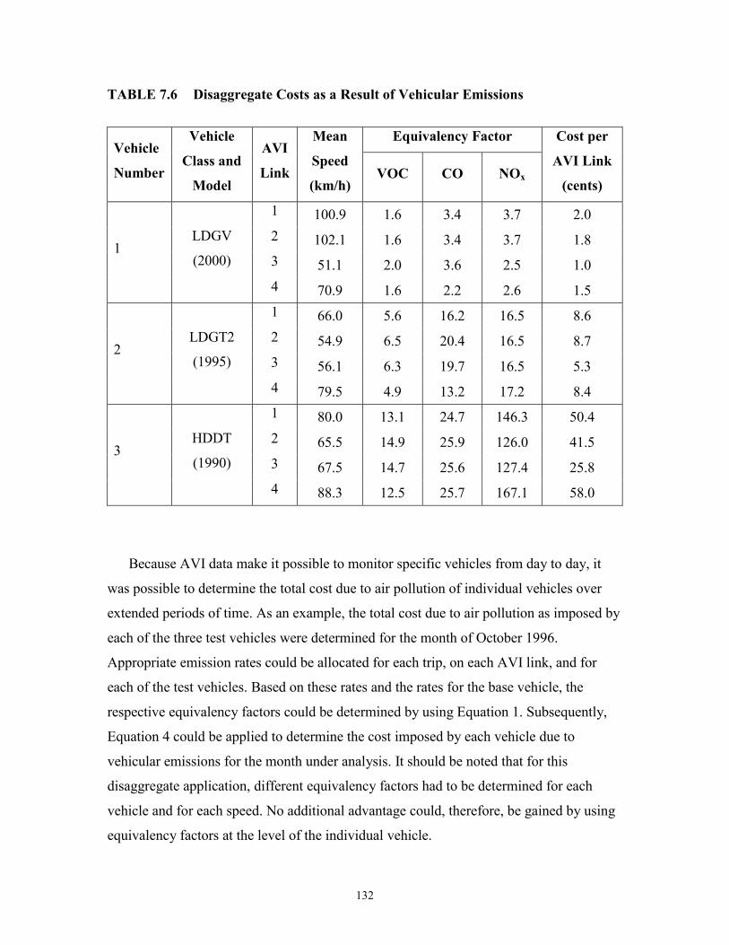
  132

TABLE 7.6  Disaggregate Costs as a Result of Vehicular Emissions 

 Equivalency Factor 

Vehicle 

Number 

Vehicle 

Class and 

Model 

AVI 

Link 

Mean 

Speed 

(km/h) VOC  CO  NOx 

Cost per 

AVI Link 

(cents) 

1  100.9  1.6  3.4  3.7  2.0 2  102.1  1.6  3.4  3.7  1.8 3  51.1  2.0  3.6  2.5  1.0 

1 LDGV 

(2000) 

4  70.9  1.6  2.2  2.6  1.5 1  66.0  5.6  16.2  16.5  8.6 2  54.9  6.5  20.4  16.5  8.7 3  56.1  6.3  19.7  16.5  5.3 

2 LDGT2 

(1995) 

4  79.5  4.9  13.2  17.2  8.4 1  80.0  13.1  24.7  146.3  50.4 2  65.5  14.9  25.9  126.0  41.5 3  67.5  14.7  25.6  127.4  25.8 

3 HDDT 

(1990) 

4  88.3  12.5  25.7  167.1  58.0  

 

  Because AVI data make it possible to monitor specific vehicles from day to day, it 

was possible to determine the total cost due to air pollution of individual vehicles over 

extended periods of time. As an example, the total cost due to air pollution as imposed by 

each of the three test vehicles were determined for the month of October 1996. 

Appropriate emission rates could be allocated for each trip, on each AVI link, and for 

each of the test vehicles. Based on these rates and the rates for the base vehicle, the 

respective equivalency factors could be determined by using Equation 1. Subsequently, 

Equation 4 could be applied to determine the cost imposed by each vehicle due to 

vehicular emissions for the month under analysis. It should be noted that for this 

disaggregate application, different equivalency factors had to be determined for each 

vehicle and for each speed. No additional advantage could, therefore, be gained by using 

equivalency factors at the level of the individual vehicle. 

  133

  It was found that vehicle one made twelve trips and resulted in a cost of only $0.88, 

vehicle two made thirteen trips and resulted in a cost of $5.55, whereas vehicle three only 

made seven trips but resulted in a cost of $11.72. Vehicle one, which is a new passenger 

car traveling at fairly high speeds, resulted in very low emissions as compared to vehicle 

three, which is a 10-year-old heavy-duty diesel truck, traveling at much lower speeds. 

Note that all of these results would change if different assumptions were used regarding 

the costs of vehicular emissions. The important point is that this methodology allows the 

allocation of responsibility at both the aggregate and disaggregate levels. In addition, this 

type of approach can be extended to form the basis of congestion pricing, which is seen 

as a very important strategy to curb congestion. 

 

CONCLUDING REMARKS   Although most transportation projects are evaluated in terms of their costs and 

benefits through net present worth analyses, the public is mostly concerned with issues 

related to sustainability such as equity, safety, and the environment. The penultimate 

phase of the proposed framework is to make decisions based on quantified performance 

measures. It was shown that a multi-criteria decision-making technique can be used to 

incorporate the concepts of sustainable transportation into the decision-making process. 

The MAUT approach was selected to analyze eleven scenarios for the widening the I-10 

corridor from three lanes to four lanes. It was illustrated that project selection could be 

markedly different if a broad range of sustainable transportation principles is considered 

instead of pure economic benefit. The level of aggregation of the input data also made a 

noticeable difference in the final project selection. The effect of analyzing the data at the 

level of AVI links as opposed to the whole corridor allowed for more flexibility in the 

allocation of weights as well as greater accuracy in the results. 

  The concept of equivalency factors can be used to assign responsibility to motorists 

for the effects of negative externalities. Equivalency factors could be used to assist in 

determining the costs imposed by vehicles due to vehicular emission On an aggregate 

level the total yearly cost imposed by each of the eight vehicle classes could be 

determined. For the disaggregate analysis, AVI data and equivalency factors could be 

used to determine the cost imposed by individual vehicles. These costs could be 

  134

determined on a trip-by-trip basis as well as for extended periods of time, such as a full 

month. It was found for example, that a ten-year-old heavy-duty diesel truck that made 

seven trips during the month imposed a cost of $11.72 as a result of air pollution, whereas 

a new passenger car that made twelve trips imposed a cost of only $0.88. Such 

applications can be used as a basis for further research into strategies such as congestion 

pricing to assist in achieving the sustainability goals of social equity and economic 

development. It should be noticed that because equivalency factors had to be determined 

for each vehicle and each speed, no additional advantage could be gained by using 

equivalency factors at the level of the individual vehicle. 

  135

CHAPTER 8: CONCLUSIONS AND FUTURE RESEARCH  

CONCLUSIONS 

  The scope of the research was such that the methodologies developed are of a generic 

nature that can be applied at both the local and network wide levels, as well as for a wide 

range of sustainable transportation performance measures. The applications, however, 

focused on mobility and environmental related performance measures for freeway 

corridors. The following are the more important findings: 

 

• While numerous qualitative studies have been performed on sustainable 

transportation there has been little quantitative research and/or implementation of 

sustainable transportation concepts. The main reasons for this are related to a lack 

of understanding of sustainable transportation and a lack of quantified 

performance measures. 

• The state of the practice of models to quantify performance is to base their 

information on aggregate data sets. Important shortcomings of this approach are 

the inaccuracies due to a loss in detail and the effect of aggregation bias. The 

latest state of the art in transportation modeling and data collection techniques, 

however, make it possible to quantify performance measures at the individual 

level, as well as a wide range of spatial and temporal aggregation. 

• A framework on how to identify, quantify, and use performance measures for 

sustainable transportation in the transportation planning process was proposed. 

The framework comprises the following five phases that are interlinked to ensure 

adequate feedback and information flow: i) identifying performance measures; ii) 

database development; iii) quantifying performance measures; iv) decision-

making; and v) implementation. 

• It was illustrated that forty percent of the regular commuterís travel times are 

statistically different to the state of the practice aggregate estimates. This result 

has significant implications for sustainability analysis and ATIS applications.  

  136

• In the case of travel time variability it was found that in approximately twenty 

percent of the cases the travel time standard deviations of the regular commuters 

are statistically different to the state of the practice aggregate estimates. 

• On a link basis it was found that travel times between links are almost exclusively 

positively correlated with only five percent of the observations indicating negative 

correlations. The results from analyzing link travel times of individual commuters 

on a trip-by-trip basis, however, revealed that individual commuters show great 

variability in travel behavior as evidenced by the fact that large tendencies to 

having both faster and slower link travel times than the aggregate estimates were 

observed. 

• A number of different types of disaggregation can be considered, namely spatial, 

temporal, combined spatial and temporal, and the individual level. The individual 

level can be used as a separate level of disaggregation or in combination with 

spatial and/or temporal disaggregation. Spatial and temporal disaggregation can 

each be applied at different levels of detail and can be defined by the segment 

lengths and time interval lengths, respectively. 

• The TRANSIMS simulation model was used to quantify a wide range of mobility 

related performance measures at various levels of spatial and temporal 

disaggregation. The uniform kernel estimator was used to smooth the erratic 

individual speed profiles produced by the TRANSIMS micro-simulator. 

• The smoothed speed profiles from the TRANSIMS micro-simulator were used 

with the MOBILE 5a model to produce vehicular emissions of individual vehicles 

on a wide range of levels of aggregation. It was shown that the effect of 

aggregation bias can be as much as twenty percent in some instances. 

• Applications such as loop detectors, AVI technology, and AVL technology could 

be simulated with TRANSIMS output. It was found that data from loop detectors 

resulted in estimates that are considerably lower than that with AVI and AVL 

technology. It is hypothesized that the reason for this is that a large percentage of 

high emitting low speeds are not accounted for with the conventional aggregate 

approach. 

  137

• A comparison was made between results with smoothed and unsmoothed speed 

profiles. It was found that both profiles produce very similar results with 

differences of less than eleven percent for all pollutant types. 

• With regard to noise pollution it was found that a twenty-two percent 

improvement could be achieved by using the shorter AVI links instead of the 

totally aggregate corridor level, as compared with the approach that uses 

interchange links. The actual values of the deviations from the approach that uses 

interchange links, however, were fairly small, with values of only 3.9 percent if 

the whole corridor is used and 2.9 percent if AVI links are used. 

• In the case of fuel consumption the effect of spatial aggregation can be fairly 

large. Average deviations from the totally disaggregate case (calculated for each 

vehicle on a second-by-second basis) of between six and sixteen percent were 

observed. It was found that incorporating the effect of the individual vehicles 

provides slightly better results. 

• It was illustrated that project selection could be markedly different if a broad 

range of sustainable transportation principles is considered instead of pure 

economic benefit. The level of aggregation of the input data also made a 

noticeable difference in the final project selection. The effect of analyzing the 

data at the level of AVI links as opposed to the whole corridor allowed for more 

flexibility in the allocation of weights, as well as greater accuracy in the results. 

• It was shown that the concept of equivalency factors can be used to assign 

responsibility to motorists for the effects of negative externalities. Equivalency 

factors could be used to allocate costs on both an aggregate and a disaggregate 

level. Such applications can be used as a basis for further research into strategies 

such as congestion pricing to assist in achieving the sustainability goals of social 

equity and economic development.  

FUTURE RESEARCH 

  This research area that deals with the quantification of performance measures for 

sustainable transportation is still relatively uncultivated. Numerous opportunities for 

further research exist due to new modeling and data collection technologies that make it 

  138

possible to quantify performance measures for sustainable transportation at the 

disaggregate level. The following needs for future research have been identified: 

 

• For this research the steps of the proposed framework were applied to freeway 

corridors. The techniques can, however, be applied to a broad range of 

transportation infrastructure. They can also be applied to geographic areas that are 

larger than corridors, such as cities and regions. A broader range of applications 

can be used to confirm the findings of this research and to obtain results for 

different scenarios. 

• For this research, AVI data and simulated data were used for quantifying the 

performance measures. There are various other types of technologies available 

that can also provide travel data at the disaggregate level. These technologies 

include global positioning systems, satellite surveillance, AVL technology, 

cellular phone technology, and various types of vehicle mounted transponders. 

The implications and benefits of using such technologies for quantifying 

performance measures for sustainable transportation should, therefore, be tested. 

• The current state of the practice in calculating vehicular emission is based on 

aggregate data sets that are used in emission models. Current simulation models 

make it possible to produce disaggregate data sets for use in emission models. The 

effect of aggregation bias, therefore, can be determined for applications in major 

metropolitan areas. This is important because such areas are currently classified in 

terms of attainment based on approaches that are prone to aggregation bias. 

• It was illustrated how equivalency factors and disaggregate data sets can be used 

to determine the costs imposed by vehicles as a result of vehicular emission. 

These techniques need to be expanded by using more comprehensive data sets and 

should also be expanded to a broader range of externalities. Such applications can 

then form the basis for further research into congestion pricing strategies. 

• Very little work has been done on developing an index for sustainable 

transportation. There is a need to augment existing work to develop an index or 

indices that would make it possible to compare the degree of sustainability 

between projects, communities, cities, and even countries. 

  139

• It was shown in this research that the travel time and the travel time variability of 

regular commuters were mostly lower than that of the aggregate estimates. These 

findings can have important implications in quantifying sustainable transportation 

performance measures for such commuters. A detailed study needs to be 

conducted by comparing the travel characteristics of regular commuters versus 

that of the general travelers. 

• It was found in this research that link travel times on an aggregate level are 

mostly positively correlated, whereas link travel times for individual commuters 

on a trip-by-trip basis were found to be mostly negatively correlated. This slow-

fast travel pattern of individual commuters needs to be studied further, because it 

has implications for modeling various effects such as emissions, noise, and fuel 

consumption. 

  140

  

 

  141

CHAPTER 9:  REFERENCES 

1.  Environmental Externalities and Social Costs of Transportation Systems: Measurement, Mitigation and Costing: An Annotated Bibliography. Federal Railroad Administration, U.S. Department of Transportation, Office of Policy, Washington D.C., August 1993. 

2.  Haq, G. Towards Sustainable Transportation Planning: A Comparison Between Britain and the Netherlands. Avebury, Aldershot, England, 1997. 

3.  Nationwide Personal Transportation Survey (NPTS). Federal Highway Administration, U.S. Department of Transportation, Office of Information, Washington D.C., 1995. 

4.  World Commission on Environment and Development (Brundtland Commission). Our Common Future. Oxford University Press, Oxford, England, 1987. 

5.  Presidentís Council on Sustainable Development. http://www.whitehouse.gov/PCSD/CSD. Accessed June 1999. 

6.  Spaethling, D. Sustainable Transportation: The American Experience. Proceedings of Seminar C: Planning for Sustainability of the 24th European Transport Forum, PTRC Education and Research Services Ltd., London, England, September 1996. 

7.  Litman, T. Issues in Sustainable Transportation. Victoria Transportation Policy Institute, Victoria, Canada, December 1999. 

8.  Lindquist, E. Moving Toward Sustainability: Transforming a Comprehensive Land Use and Transportation Plan. In Transportation Research Record 1617, Transportation Research Board, National Research Council, Washington D.C., 1998, pp. 1-9. 

9.  Masser, I., O. Sviden, and M. Wegener, Transport Planning for Equity and Sustainability. Transportation Planning and Technology, Vol. 17, Gordon and Breach Science Publishers, Loughborough, England, 1993, pp. 319-330. 

10.  Peake, S., and C. Hope. Sustainable Mobility in Context: Three Transport Scenarios for the UK. Transport Policy, Vol. 3, Butterworth-Heinemann Ltd, Oxford, England, 1994, pp. 195-207. 

11.  Reid, D. Sustainable Development: An Introductory Guide. Earthscan Publications Ltd., London, England, 1995. 

12.  Dittmar, H. Thinking Like a System: Sustainability Through Transportation Technology. ITS Quarterly, Vol. 4, No. 1, Washington D.C., Winter 1996, pp. 19-26. 

13.  Akinyema, E. O. A Total Performance Approach to Traffic Management for Sustainable Development of Communities in Third World Cities. Proceedings of the National Conference held in Tampa Florida on Transportation and Sustainable Communities, Institute of Transportation Engineers, Washington D.C., 1997. 

  142

14.  Mickelson, R. P. Synthesis of Highway Practice 267: Transportation Development Process. National Cooperative Highway Research Program, Transportation Research Board, National Research Council, Washington D.C., 1998. 

15.  Gatersleben, B. Sustainable Transportation and Quality of Life. Proceedings of the Conference on Social Change and Sustainable Transportation (SCAST), held at the University of California at Berkeley, March 1999. 

16.  Transportation and Sustainable Communities Initiative: Overview of Federal Sustainable Transportation Activities. National Science and Technology Council, Subcommittee on Transportation Research and Development, Washington D.C., June 1998. 

17.  Sustainability Indicators: The Transportation Sector. Ontario Roundtable on Environment and Economy, IndEco Report 94029, Toronto, Canada, September 1995. 

18.  National Transportation System Performance Measures. Report Prepared for the Office of the Secretary of the U.S. Department of Transportation, Washington D.C., April 1996. 

19.  Gardner, K., and J. Carlsen. Performance Indicators for Sustainable Transport in London. Proceedings of Seminar C: Planning for Sustainability, PTRC European Transport Forum, Brunel University, England, September 1996. 

20.  A Guide to Metropolitan Transportation Planning Under ISTEA ñ How the Pieces Fit Together. Federal Transit Administration, U.S. Department of Transportation, Washington D.C., 1997. 

21.  TEA-21: Moving Americans into the 21st Century, U.S. Department of Transportation. http://www.fhwa.dot.gov/tea21/index.htm. Accessed January 1999. 

22.  Codd, N., and C. M. Walton. Performance Measures and Framework for Decision Making Under the National Transportation System. In Transportation Research Record 1518, Transportation Research Board, National Research Council, Washington D. C., 1996, pp.70-77. 

23.  Zietsman, J. and L.R. Rilett. Analysis of Aggregation Bias in Vehicular Emission Estimation Using TRANSIMS Output. In Transportation Research Record 1750, Transportation Research Board, National Research Council, Washington D.C., 2001, pp 56-63. 

24.  Ortuzar, J de D., and L. G. Willumsen. Modelling Transport: Second Edition. John Wiley and Sons, New York, December 1995. 

25.  Smith, L., R. Beckman, D. Anson, K. Nagel, and M.E. Williams. TRANSIMS: Transportation Analysis and Simulation System. Proceedings of the Fifth National Conference on Transportation Planning Methods and Applications held in Seattle, April 1995. 

  143

26.  Alexander, E. R., E. A. Beimborn, C.V. Patton, and L. P. Witzling. Multi-Objective Decision Making for Transportation. Bureau of Policy & Planning, Wisconsin Department of Transportation, Milwaukee, Wisconsin, November 1985. 

27.  Meyer, M. D., and E. J. Miller. Urban Transportation Planning: A Decision-Oriented Approach. McGraw-Hill, New York, 1984. 

28.  Nijkamp, P. Roads Towards Environmentally Sustainable Transport. Transportation Research Part A. Vol. 28A, No. 4, Elsevier Science Ltd., Oxford, England, 1994, pp. 261-271. 

29.  Litman, T. Sustainable Transportation Indicators. Victoria Transportation Policy Institute, Victoria, Canada, July 1997. 

30.  Ewing, R. Beyond Speed: The Next Generation of Transportation Service Standards. Annual meeting of the Institute of Transportation Engineers, Compendium of Technical Papers, Washington D.C., 1992. 

31.  Pratt, R. H., and Lomax T. J. Performance Measures for Multimodal Transportation Systems. In Transportation Research Record 1518, Transportation Research Board, National Research Council, Washington D. C., 1996, pp. 85-93. 

32.  The ì Sî  Factor: Increasingly, Companies are Viewing Sustainability as a Business Issue. The Hands-on Journal for Environmentally Conscious Companies, Washington D.C., June 1998, pp. 1-8. 

33.  Mckee, M., T. W. Morgan, R. Narayanan, and A. B. Bishop. A Methodology for Public-Planner Interaction in Multiobjective Project Planning and Evaluation. Water Resources Planning Series, Utah State University, Logan, Utah, December 1981. 

34.  Toward a Sustainable Future: Addressing the Long-Term Effects of Motor Vehicle Transportation on Climate and Ecology. Special Report 251, Transportation Research Board, National Research Council, Washington D.C., 1997. 

35.  Towards Sustainable Transportation. Proceedings of OECD Conference, Vancouver, Canada, March 1996. 

36.  Livable Communities. http://www.house.gov/blumenauer/livable.htm. Accessed November 1999. 

37.  Ruckelshaus, W. D. Toward a Sustainable World. Scientific American, No. 261, New York, 1989, pp.166-170. 

38.  Pearce, D. Blueprint 3: Measuring Sustainable Development. Earthscan, London England, 1993. 

39.  Sustainable Transportation: Priorities for Policy Reform. The World Bank, Washington D.C., 1996. 

  144

40.  Towards a Sustainable Future. Special Report 251, Transportation Research Board, National Research Council, Washington D.C., 1997. 

41.  European Foundation for the Improvement of Living and Working Conditions. http://susdev.eurofound.ie. Accessed January 2000. 

42.  Moving on Sustainable Transportation (MOST). http://www.tc.gc.ca/envaffairs/most. Accessed January 2000. 

43.  Sperling, D., and S. A. Shaheen. Transportation and Energy: Strategies for a Sustainable Transportation System. Institute of Transportation Studies, University of California, Berkeley, 1995. 

44.  Houghton, N. Ecologically Sustainable Development: Indicators and Decision Process. Report 319, ARRB Transportation Research, Vermont South, Australia, March 1998. 

45.  Hohmeyer, O. Social Costs of Climate Change Strong Sustainability and Social Costs. Proceedings of a Conference Held in Ladenburg, Springer, Berlin, Germany, May 1995. 

46.  Pocket Guide to Transportation. Bureau of Transportation Statistics, U.S. Department of Transportation, Washington D.C., December 1998. 

47.  Schiller, P., and B. de Lille. Green Streets: The 1991 Intermodal Surface Transportation Efficiency Act and the Greening of Transportation Policy in the United States. Surface Transportation Policy Project, Washington D.C., 1997. 

48.  McDowell, B. D. Reinventing Planning Under ISTEA: MPOís and State DOTís. Transportation Research Board, National Research Council, Washington D.C., November 1994. 

49.  Air Quality Demands on Transportation Planning in Texas. A White Paper Prepared by the Technical Working Group for Mobile Source Emissions, Austin, Texas, August 1998. 

50.  Bass, P., D. Perkinson, B. Keitgen, and G. Dresser. The Context of Analysis (ISTEA and the Clean Air Act). Report 1235-14, Texas Transportation Institute, College Station, Texas, 1994. 

51.  Anderson, J. E. Public Policymaking: An Introduction: Second Edition. Houghton Mifflin Company, Boston, 1994. 

52.  Mason, D. Subsidiarity Wins Over Sustainability Every Time. Surveyor, Vol. 181, No. 5280, Hemming Group Ltd, London, England, February 1994, p. 12. 

53.  Richardson, E., D. Rice, and C. Jelly. Urban Transport for a Vital and Sustainable Future. Road and Transport Research, Vol. 2, No. 2, Victoria, Australia, June 1993, pp. 58-68. 

54.  Deakin, E. Policy Responses in the USA. Transport, the Environment, and Sustainable Development. Contained in Transport, the Environment, and 

  145

Sustainable Development. Edited by Banister, D., and K. Button, E & FN Spon, London, England, 1993. 

55.  Ewing, R., Measuring Transportation Performance. Transportation Quarterly. Vol. 49, No. 1, Washington D.C., Winter 1995, pp. 91-104. 

56.  Better Understanding our Cities: The Role of Urban Indicators. Organization for Economic Co-operation and Development, Paris, France, 1997. 

57.  Poister, T. H. Performance Measures in State Departments of Transportation. National Cooperative Highway Research Program, Synthesis of Highway Practice, No. 238, Transportation Research Board, National Research Council, Washington D. C., 1997. 

58.  Hart, M. Hart Environmental Data: Indicators of Sustainability. http://www.subjectmatters.com/indicators/index.html. Accessed December 1998. 

59.  Indicators of the Environmental Impacts of Transportation: Highway, Rail, Aviation, and Maritime Transport. Report 230-R-96-009, Environmental Protection Agency, Washington D.C., October 1996. 

60.  Lomax, T. J., S. M. Turner, and G. Shunk. Quantifying Congestion: Final Report and Userís Guide. Report 398, National Cooperative Highway Research Program, Washington D.C., 1997. 

61.  Black, W. R. Toward a Measure of Transport Sustainability. Proceedings of the 79th Annual Meeting of the Transportation Research Board, National Research Council, Washington D.C., January 2000. 

62.  Stuart, D. G. Goal-Setting and Performance Measurement in Transportation Planning and Programming. Journal of Transportation, Vol. 1, No. 2, Tampa, Florida, Winter 1997, pp. 49-72. 

63.  Rennings, K. Economic and Ecological Concepts of Sustainable Development: External Costs and Sustainability Indicators. Proceedings of a Conference Held in Ladenburg, Springer, Berlin, Germany, May 1995. 

64.  National Transportation System Performance Measures. Report prepared for the Office of the Secretary of the U.S. Department of Transportation, Washington D.C., April 1996. 

65.  Lomax, T. J., and D. L. Schrank. The Keys to Estimating Mobility in Urban Areas, Applying Definitions and Measures that Everyone Understands. Texas Transportation Institute, The Texas A&M University System, College Station, Texas, January 1999. 

66.  Abrams, C. M., and J. F. DiRenzo. Measures of Effectiveness for Multimodal Urban Traffic Management, Volume 2: Development and Evaluation of TSM Strategies. Report FHEA-RD-79-113 Federal Highway Administration, U.S. Department of Transportation, Washington D.C., 1979. 

67.  Turner, S. M., M. E. Best, and D. L. Schrank, Measures of Effectiveness for 

  146

Major Investment Studies. Report SWUTC/96/467106-1, Southwest Region University Transportation Center, Texas A&M University System, College Station, Texas, 1996. 

68.  Guyton, J. W. Presentation of Comparative Data for Transportation Planning Studies. In Transportation Research Record 1617, Transportation Research Board, National Research Council, Washington D.C., 1998, pp. 44-49. 

69.  McLeod, D. S. Special Features of Floridaís Mobility Management Process. In Transportation Research Record 1552, Transportation Research Board, National Research Council, Washington D.C., 1996, pp. 42-47. 

70.  Florida Recommended Mobility Performance Measures. Memorandum prepared by the Florida Department of Transportation, Tallahassee, Florida, July 1998. 

71.  Landau, U. Aggregate Prediction with Disaggregate Models: Behavior of the Aggregation Bias. In Transportation Research Record 673, Transportation Research Board, National Research Council, Washington D. C., 1974, pp. 100-105. 

72.  McFadden, D., and F. Reid. Aggregate Travel Demand Forecasting from Disaggregate Behavioral Models. In Transportation Research Record 534, Transportation Research Board, National Research Council, Washington D. C., 1975, pp. 24-37. 

73.  Koppelman, F. S. Prediction with Disaggregate Models: The Aggregation Issue. In Transportation Research Record 527, Transportation Research Board, National Research Council, Washington D. C., 1974, pp. 73-80. 

74.  Tye, W. B., L. Sherman, M. Kinnucan, D. Nelson, and T. Tardiff. Applications of Disaggregate Travel Demand Models. Report 253, National Cooperative Highway Research Program, Transportation Research Board, National Research Council, Washington D. C., 1982. 

75.  Benjamin J. R., and C. A. Cornell. Probability, Statistics, and Decision for Civil Engineers. McGraw-Hill, New York, 1970. 

76.  Reid, F. A. Minimizing Error in Aggregate Predictions from Disaggregate Models. In Transportation Research Record 673, Transportation Research Board, National Research Council, Washington D.C., 1974, pp. 59-64. 

77.  Eisele, W. L., S. M. Turner, and R. J. Benz. Using Acceleration Characteristics in Air Quality and Energy Consumption Analysis. Report SWUTC/96/465100-1, Southwest Region University Transportation Center, Texas A&M University System, College Station, Texas, August 1996. 

78.  Quiroga, C. A., and D. Bullock. Travel Time Studies With Global Positioning and Geographic Information Systems: An Integrated Methodology. Transportation Research Part C, Vol. 6, Elsevier Science Ltd, Exeter, England, 1998, pp. 101-127. 

79.  Bush, B. W. The TRANSIMS Framework. Report LA-UR-99-7, Los Alamos 

  147

National Laboratory, Los Alamos, New Mexico, 1999. 

80.  Rilett, L. R. Transportation Planning and the TRANSIMS Micro-simulation Model: Prepared for the Transition, Preprint, 80th Annual Meeting of the Transportation Research Board, Washington D. C., 2000. 

81.  Nagel, K., P. Stretz, M. Pieck, S. Lecky, R. Donnelly, and C. L. Barrett. TRANSIMS Traffic Flow Characteristics. Report LA-UR-97-3530, Los Alamos Nation Laboratory, Los Alamos, New Mexico, July 1997. 

82.  United States Environmental Protection Agency (EPA). http://www.epa.gov/. Accessed January 1999. 

83.  Crawford, J. A., C. Jordan, and G. B. Dresser. Modal Emissions Modeling with Real Traffic Data. Report 1358-3F, Texas Transportation Institute, The Texas A&M University System, College Station, Texas, January 1999. 

84.  Jordan, D. C. Measures of Responsibility for Pollution and their Application in Road Pricing. Master of Science Thesis, University of Alberta, Canada, 1996. 

85.  New Highway Traffic Noise Prediction Model Almost Complete, Federal Highway Administration, U.S. Department of Transportation. http://www.tfrc.gov/trnsptr/rttmar96/rd960065.htm. Accessed January 1999. 

86.  McTrans: Center for Microcomputers in Transportation. http://www.mctrans.ce.ufl.edu/. Accessed April 2000. 

87.  Highway Capacity Manual. Special Report 290, Transportation Research Board, National Research Council, Washington D.C., 1997. 

88.  Dixon, M. P. Incorporation of Automatic Vehicle Identification Data Into the Synthetic OD Estimation Process. Ph.D. Dissertation, Texas A&M University, College Station, Texas, May 2000. 

89.  Fu, L., and L. R. Rilett. Expected Shortest Paths in Dynamic and Stochastic Traffic Networks. Transportation Research Part B, Vol. 32, No. 7, 1998, Elsevier Science Ltd., Exeter, England, 1998, pp. 449-516. 

90.  Rilett, L. R., K. Kim, and B. Raney. A Comparison of the Low Fidelity TRANSIMS and High Fidelity CORSIM Highway Simulation Models Using ITS Data. Preprint 00-0678, Transportation Research Board 79th Annual Meeting, Washington D. C., January, 2000. 

91.  Cleveland, W.D., and S.J. Devlin. Locally Weighted Regression: An Approach to Regression Analysis by Local Fitting. Journal of the American Statistical Association, Vol. 83, No. 403, New York, September 1988. 

92.  Perkinson, D. G., C. Bell, and G. B. Dresser. Development of Gridded Mobile Source Emissions Estimates for the Houston-Galveston Nonattainment Counties FY 2007 in Support of the COAST Project. Report 402001, Texas Transportation Institute, The Texas A&M University System, College Station, Texas, December 1998. 

  148

93.  Jordan, D. C. Measures of Responsibility for Pollution and their Application in Road Pricing. Master of Science Thesis, University of Alberta, Canada, 1996. 

94.  Jordan, D. C., J. Zietsman, and L. R. Rilett. Development of Sustainable Transportation Metrics for Vehicular Pollutants. Transportation Planning and Technology, Volume 24, No. 3. Leicestershire, England, 2001, pp 86-94. 

95.  Turner, S.M., B. J. Gajewski, and G. B. Dresser. Sensitivity of Analysis Time Intervals for Mobile Source Emissions Estimation: Using Archived ITS Data to Determine Effects on VKT-Speed Distributions and Emissions Estimates. Preprint, Transportation Research Board 80th Annual Meeting, Washington D. C., January, 2001. 

96.  Zietsman, J., and L. R. Rilett. Using TRANSIMS and ITS Data to Quantify Aspects of Sustainable Transportation. Proceedings of the 9th World Conference on Transportation Research, Seoul, Korea, July 2001.  

97.  Guidelines for Analysis and Abatement of Highway Traffic Noise. Texas Department of Transportation, Environmental Affairs Division, Austin, Texas, June 1996. 

98.  Rao, K. S., and R. A. Krammes. Energy-Based Fuel Consumption Model for FREFLO. In Transportation Research Record 1444, Transportation Research Board, National Research Council, Washington D. C., 1994, pp. 36-43. 

99.  Olson, D. L. Decision Aids for Selection Problems. Springer, New York, 1996. 

100.  Rilett, L. R. Allocating Pollution Costs Using Noise Equivalency Factors. In Transportation Research Record 1498, Transportation Research Board, National Research Council, Washington D. C., 1996, pp. 102-107. 

101.  Rilett, L. R., B. G. Hutchinson, and R .C. G. Haas. Cost Allocation Implications of Flexible Pavement Deterioration Models. In Transportation Research Record 1215, Transportation Research Board, National Research Council, Washington D.C., 1988, pp. 31-42. 

102.  AASHTO Road Test: Report 5- Pavement Research. Special Report 615. American Association of State Highway Transportation Officials (AASHTO), Highway Research Board, Washington D.C., 1962. 

103.  Irwin, N. Transportation Pricing Strategies to Recover Environmental Costs. Annual Conference on Building Environmental Externalities into Full-cost Accounting, Transportation Association of Canada, Prince Edward Island, Canada, October 1996. 

104.  Litman, T. Transportation Cost Analysis for Sustainability. Victoria Transport Policy Institute, Victoria, Canada, July 1996. 

105.  Whitelegg, J. Transportation for a Sustainable Future: The Case for Europe. Belhave Press, London, England, 1993. 

106.  Zegras, C., and T. A. Litman. Cost Estimates of Transportation Air Pollution in 

  149

Santiago, Chile. In Transportation Research Record 1587, Transportation Research Board, National Research Council, Washington D.C., 1997, pp. 106-112. 

107.  Tellis, R. and C. J. Khisty. Congestion Pricing: The Actual Cost to Drive an Automobile on Urban Highways. Proceedings of the 1995 ASCE Conference, American Society of Civil Engineers, Reston, Virginia, 1995, pp. 946-957. 

108.  Irwin, N. Transportation Pricing Strategies to Recover Environmental Costs. Annual Conference on Building Environmental Externalities into Full-cost Accounting, Transportation Association of Canada, Prince Edward Island, Canada, October 1996. 

109.  Delucchi, M. A. Total Cost of Motor-Vehicle Use. Access No. 8, University of California Transportation Center, Berkeley, California, Spring 1996.