Synthesis of Spatially & Temporally Disaggregate …alaink/Orf467F12/NJ... · 1 synthesis of spatially & temporally disaggregate person trip demand: application for a typical new

1

SYNTHESIS OF SPATIALLY & TEMPORALLY DISAGGREGATE

PERSON TRIP DEMAND:

APPLICATION FOR A TYPICAL NEW JERSEY WEEKDAY

Talal R. Mufti

Adviser: Alain L. Kornhauser

DRAFT COPY

Submitted in partial fulfillment of the

requirements for the degree of Master of

Science in Engineering

Department of Operations Research and

Financial Engineering

Princeton University

November 2012

2

I hereby declare I am the sole author of this thesis.

Talal R Mufti

I authorize Princeton University to lend this thesis to other institutions or individuals for the

purpose of scholarly research.

Talal R Mufti

I further authorize Princeton University to replicate this thesis by photocopying or by other means,

in total or in part, at the request of other institutions or individuals for the purpose of scholarly

research.

Talal R Mufti

3

ABSTRACT With the advent of technologies such as autonomous taxis and large-scale personal rapid transit

networks drawing nearer to the present reality, serious studies must be made with regard to what

levels of demand and opportunity exist for the degree of accessibility that such technologies can

provide in urban areas. With a lack of high resolution information available from conventional

surveying methods, this thesis looks to generate synthetic data regarding person trips at a highly

disaggregated level, in space and in time, across the entire state of New Jersey. The model used

produces an output of 32.6 million trips where the average trip distance, after removing outliers, is

12.4 miles and the average travel time to work is 21 minutes—figures that are reasonably near to

New Jersey benchmarks. The thesis documents the model’s methodologies and results and

proceeds to display limitations as well as suggest improvements for future iteration.

4

Table of Contents Abstract ....................................................................................................................................................................................... 3

List of Figures ............................................................................................................................................................................ 5

List of Tables .............................................................................................................................................................................. 6

Introduction .......................................................................................................................................................................... 7

Motivation .............................................................................................................................................................................. 7

Background ........................................................................................................................................................................... 8

Scope ........................................................................................................................................................................................ 8

Goals ......................................................................................................................................................................................... 9

Some Terminology ............................................................................................................................................................. 9

History and State of the Art ............................................................................................................................................... 11

Early Travel Demand Models....................................................................................................................................... 11

Activity-Based Models .................................................................................................................................................... 12

Methodology: ........................................................................................................................................................................... 13

Predictable Activities & Others Trips ....................................................................................................................... 13

Fundamental Assumptions ........................................................................................................................................... 13

Task 1: Generating the Populace ................................................................................................................................ 17

Task 2: Assigning Work Places to Workers ........................................................................................................... 23

Task 3: Assigning Schools and other Educational Institutions ...................................................................... 28

Task 4: Assigning Activity Patterns ........................................................................................................................... 32

Task 5: Assigning Destinations for Other Trips ................................................................................................... 34

Task 6: Adding the Temporal Dimension ............................................................................................................... 39

Data ............................................................................................................................................................................................. 43

2010 Census Summary File 1 Data ............................................................................................................................ 44

American Community Survey ...................................................................................................................................... 49

School Data Sets ................................................................................................................................................................ 49

Employers and Patronage Data .................................................................................................................................. 50

Schedule Files ..................................................................................................................................................................... 51

Data for Future Projects ................................................................................................................................................. 52

Results ........................................................................................................................................................................................ 53

Attributes of the Synthetic Population and its Workers................................................................................... 53

Household Income and Work Industries ................................................................................................................ 58

Student Populations Numbers .................................................................................................................................... 60

5

Activity Pattern Distributions ..................................................................................................................................... 61

Commute Times and Trip Distance Distributions ............................................................................................... 63

Conclusions, Limitations, and Next Steps .................................................................................................................... 67

Task 1..................................................................................................................................................................................... 67

Task 2..................................................................................................................................................................................... 68

Task 3..................................................................................................................................................................................... 69

Task 4..................................................................................................................................................................................... 70

Task 5..................................................................................................................................................................................... 70

Task 6..................................................................................................................................................................................... 71

Other Possible Improvements ..................................................................................................................................... 71

Bibliography ............................................................................................................................................................................ 73

Appendices ............................................................................................................................................................................... 77

Random Draw Functions ............................................................................................................................................... 77

Links to Synthesizer Code and Other Scripts ........................................................................................................ 78

LIST OF FIGURES Figure 1 Process Chart of Task 1 Methods .................................................................................................................. 20

Figure 2 Population Hierarchy ......................................................................................................................................... 21

Figure 3 Sample Output of Module 1 ............................................................................................................................. 22

Figure 4 Process Chart of Task 2 Methods for non-NJ Counties ........................................................................ 23

Figure 5 Process Chart of Task 2 Methods for NJ ..................................................................................................... 26

Figure 6 Sample Output of Module 2a which generates out-of-state workers ............................................ 26

Figure 7 Sample Output of Module 2c which adds work attributes to out-of-state workers ................ 26

Figure 8 Sample Output of Module 2b .......................................................................................................................... 27

Figure 9 Process Chart of Task 3 Methods .................................................................................................................. 28

Figure 10 Sample Output of Module 3 .......................................................................................................................... 31

Figure 11 Process Chart of Module 4 ............................................................................................................................ 34

Figure 12 Process chart of Module 5 ............................................................................................................................. 36

Figure 13 Sample Output of Module 5. ......................................................................................................................... 37

Figure 14 Visualizing Trip Filaments Using a Google Earth Application ........................................................ 39

Figure 15 Process Chart of Module 6 ............................................................................................................................ 40

Figure 16 Tree Structure of Folders Relevant to Synthesizer ............................................................................. 43

Figure 17 Census Block Boundaries and their Centroids for Atlantic County ............................................. 45

Figure 18 Plot of sorted Land Area for all blocks in NJ .......................................................................................... 46

Figure 19 After cutting off tail at y=120000 ............................................................................................................... 46

Figure 20 Populations by County and Sex from Synthesizer Output ............................................................... 56

Figure 21 Populations by County and Sex from 2010 Census ............................................................................ 56

6

Figure 22 CDF of Synthesized Population by Age and Sex for NJ ...................................................................... 57

Figure 23 CDF of Population by Age Ranges and Sex for NJ from 2010 Census .......................................... 57

Figure 24 Household Incomes for Synthesized Population ................................................................................. 58

Figure 25 Household Income Brackets from ACS 2010 ........................................................................................ 59

Figure 26 Workers by Travel Time to Work for New Jersey and United States (2000) (DMJM Harris,

Inc, 2006) .................................................................................................................................................................................. 64

Figure 27 Commute Times of Non-Homeworker, Non-Student Workers over 16 ..................................... 64

Figure 28 Histogram of Distances under 70 miles .................................................................................................. 66

Figure 29 Histogram of Distances under 10 miles .................................................................................................. 66

LIST OF TABLES Table 1 Codes for Traveler Types, Household Types, and Income Brackets ................................................ 17

Table 2 Out-of-State Locations and Categorizations ............................................................................................... 23

Table 3 Industry Codes used in Module 2 ................................................................................................................... 24

Table 4 Activity Patterns .................................................................................................................................................... 32

Table 5 Probability Distributions of Activity Pattern by Traveler Type ......................................................... 33

Table 6 Neighboring (1-adjacent) Counties ............................................................................................................... 35

Table 7 Output Fields by Module ordered by Field Index. Note that Module 6 inserts new fields

rather than appending them. ............................................................................................................................................ 41

Table 8 2010 Census SF 1 Data Used in Task 1 ......................................................................................................... 47

Table 9 County Populations: Output and Census Numbers ................................................................................. 53

Table 10 Number of Out-of-State Workers ................................................................................................................. 54

Table 11 Number of Workers in Output and QWI data ......................................................................................... 54

Table 13 Student Type distributions of Synthesized Population and ACS 2010......................................... 60

Table 14 Probability Distributions of Activity Pattern by Traveler Type as Calculated from

Synthesizer Output ............................................................................................................................................................... 61

Table 15 Percentages of Trip Types from Synthesizer Output and from Trip Chaining Summary

Statistics .................................................................................................................................................................................... 62

Table 16 Percentiles of Distances of Synthesized School Trips ......................................................................... 65

Table 17 Percentiles of Distances of all Synthesized Trips .................................................................................. 65

7

INTRODUCTION

“PRT is the Technology of the Future… And it always will be.” - Anonymous

Transportation is a vital service to every sector of the economy of any nation. The need for

individuals and organizations to travel quickly to exact locations, and hence the primary need for

transportation, has long been identified as an inherently derived demand, and not an end in and of

itself (Jones, 1979). It has been several decades now since this notion of travel as a derivative of

human behavior and activity has been more deeply explored and utilized in transportation models.

However, it is this past decade's ready availability of fast processors and large inexpensive memory

that have allowed the emergence of many highly complex models.

In 2010, New Jersey (NJ) was the second highest (FTA, 2010) recipient of ARRA (American

Recovery and Reinvestment Act) funding and the 6th highest (FTA, 2010) recipient of non-ARRA

funds and grants from the US Department of Transportation (DOT). It is evident that great lengths

have been taken by the NJDOT—the first State DOT—and regional planners to develop the

infrastructures for both motorized vehicles, as well as other transit systems such as rail and light-

rail. The latter alone meets only the demand to and from very specific locations. Supplemented with

the automobile’s ubiquitous accessibility, such spatial aggregation was tolerable. It becomes

intolerable, however, when dealing with systems with accessibility at very few specific locations

relative to the multitude of places where it is needed.

MOTIVATION Despite a significant pouring of resources and funding by the New Jersey Transit Corporation,

NJDOT’s “operating arm,” Mass Transit in New Jersey still serves a relatively small share of the

market. Nationally, transit only serves “about 2% of all motorized trips” (Kornhauser, 2012). It has

become apparent that currently available transit systems simply cannot compete with personal

automobiles, especially in suburban areas. The figure above rises slightly to about 5% (McKenzie &

Rapino, 2011) in the best case scenario of daily commuting. This supports the common reasoning

that with enough aggregation at two points, A and B, in a short enough span of time, Mass Transit

becomes more viable. Conversely, when the A’s and B’s are distributed very broadly in both space

and time, the likelihood of finding A,B pairs which can be adequately and feasibly serviced by mass

transit diminishes rapidly, as is the case currently. The automobile, however, can readily serve such

trips with less agony than transit, generally acceptable travel times even in congestion, ability to

service precise locations, as well as and due to the utilization of extensive existing roadway

infrastructure. That is to say, it outdoes transit because of its ubiquitous accessibility and its ability

to serve individual trips, all at a cost that most are willing to pay.

To compete against all the strengths of the automobile, transit must first and foremost increase its

accessibility while remaining fast and economical. This requires a two-pronged approach:

significantly reducing the cost of the “driver” and accessibility through a more extensive network

that would service a great percentage of urban and suburban travel demand. Today advancements

in technology, both existing and on the horizon, can make both of these possible. Several successful

proof-of-concept Personal Rapid Transit (PRT) systems have emerged in recent years (Adanced

Transit Applications, 2012). Such systems’ relatively compact and inexpensive guideway, and

intelligent pod allocation could meet both demands stated above. More promising still, is the

8

prospect of Automated Taxis Systems that could simply utilize the existing roads and highways. The

advent of such technologies, however, will require a much better and more detailed understanding

of where exactly people want to go. Models without sufficient spatial disaggregation are of little use

since they do not have the specificity to determine the true level of accessibility being provided to

users. If a traveler has to walk more than, say, a quarter-mile to reach an access point, such as a PRT

station, then he/she is more likely to forgo the option altogether. Determining where exactly to

place access points to meet demand is pivotal in competing with the automobile, and doing so

requires information and a level of detail that no current surveys can provide.

BACKGROUND There are several organizations that oversee the planning of the state’s transportation

infrastructure and that create the models on which decisions are based. While the chief decision

maker is the NJDOT, much of the modeling and planning is done by the three Metropolitan Planning

Organizations (MPO) in the region, namely the North Jersey Transportation Planning Association,

presiding over the 13 northernmost counties, the South Jersey Transportation Planning

Organization for the four southernmost counties, and the Delaware Valley Regional Planning

Committee (DVRPC) for the remaining four counties in addition to some outside NJ. Currently all

three use transportation models based on the classic but still-popular 4-step process, though the

DVRPC has recently begun creating an AB model as of January 2012. . Most activity-based (AB)

models first emerged in Europe, but they are now reaching a point of maturity across the developed

world and will likely become the dominant paradigm in travel forecasting and transportation

planning, especially in larger metropolitan regions (Puchalsky, 2012).

Such models are meant for both analysis and forecasting. Doing the latter accurately would require

a significant amount of time and energy for development, calibration and validation—the DVRPC's

new model is currently expected to be ready in three years’ time (Puchalsky, 2012) for example and

it is unclear how well–geared it will be to studying the possibility of Advanced Transit Systems.

SCOPE A model that instead localizes the temporal dimension of the model to a single day is substantially

easier and more feasible for the purposes of a single person project. Furthermore, the level of detail

which such a model provides allows for highly-useful, albeit synthetic, data about travel at a spatial

resolution that is otherwise unattainable.

As such, creating a simulation that synthesizes a permutation of all trips that occur in day through

the state of New Jersey was considered a feasible low-hanging fruit to address and work on. Later

sections in this thesis will discuss the extensibility of this project—other fruit to be picked—as well

as other branches, which all belong to the same tree—a potentially comprehensive and integrated

activity-based transportation demand analysis and forecasting model. The majority of this thesis

deals with the project at hand, which integrates large amounts of demographic, employment,

industry, school, and human behavioral data to create a high-resolution snapshot of travel demand,

via each individual trip made by each individual NJ resident and each individual out-of-state

commuter that works in New Jersey.

9

GOALS Once again, the goal of the synthesizer is to generate the precise origin, destination, and

arrival/departure time for every trip made by every individual on a typical workday when school is

in session. More simply, it is a look into where residents and visitors to the state go on a typical day

and when. Every individual run of the synthesizer produces a unique trip file that contains an

individualized, probabilistic record of every person-trip on an average weekday, which is expected

to total to just over 30 million trips. Each record includes every trip the person makes including

spatial coordinates of the origins and destinations as well as the exact departure and arrival times

in seconds after midnight, as well as pointers into relevant files listing places of interest such as

schools and work places.

SOME TERMINOLOGY Among the plethora of papers, reports and theses in the area of transportation demands

models, there are at least a few terms which tend to be used with slightly different meanings or

nuances in the minds of different authors. Here we define a few of these terms for the purpose of

clarity and unambiguous use throughout this paper. Many of these terms will be elaborated on as

necessary and new terms will be introduced as needed in the relevant sections below.

• Trip A single movement of a person from an origin to a destination, independent of mode of travel

or other trips.

• Tour or Trip Chain A tour is typically considered a set of consecutive trips, thought of here as a

multiple stop tour starting at home, usually in the morning, and returning home sometime later in

the day. Since the Synthesizer does not deal with Mode Assignment, the term tour is used to be

synonymous with trip-chain, which is simply the chain of trips a single person goes on

throughout the day. The distinction between these definitions and those of the National Household

Travel Survey are made in the section on

10

Activity Pattern Distributions.

• Activity Pattern or Tour Type A particular tour, assigned to a generated person, that determines

his/her activities, and therefore trips, for the day.

• Home Worker This is used as a blanket term for persons generated such that they do not travel

to work or school that day. This includes many possible types of residents include the

unemployed, self-employed, those taking a sick-day off, or even the elderly or infants.

• Other Trips that are made to or from any place other than home, school or work. If prefaced

with Homebased or Workbased, this implies the origin of the trip is home or work respectively.

• Householder The ‘head’ of the household, or simply the first adult resident to be placed by the

Synthesizer in a household.

11

HISTORY AND STATE OF THE ART A Glimpse at 60 Years of Transportation Demand Modeling

What follows is a brief history of travel demand modeling citing a short selection of important

literature to chronicle the field's evolution from simplistic statistically-oriented trip-based

modeling to current behaviorally-oriented activity-based modeling and the state of the art.

EARLY TRAVEL DEMAND MODELS Following the end of the Second World War, the boom in the American automobile industry, and

the Federal-Aid Highway Acts of 1934, 1944, and 1956, transportation planning models seemed

more needed than ever. Personal motorized vehicles were no longer just pleasure vehicles but

rather a significant and rapidly-growing mode of transport (Weiner, 1992). Some of the earliest

attempts to forecast and model this growth and its effect on regional land-use and mobility can be

dated even further back to the late 1920s—the Boston Transportation Study of 1926 saw the use of

a rudimentary gravity model to forecast traffic. The field steadily grew, finally achieving critical

mass in the early 1960's through the help of greater funding and the availability of non-military

computers with which to process large amounts of data (Southworth, 1995). A Model of Metropolis

(Lowry, 1964) and other works built upon it were among the first attempts at an urban model for

travel demand and land-use characteristics like population and employment.

Trip-based travel demand models, much like the one used by Lowry, came to be the most

popular and widely-used for several decades to come. They were centered around single

purpose single destination trips and, at first, only considered trips to work and home. Such models

essentially all followed the same paradigm of four sequential steps: trip generation, trip

distribution, mode split, and route assignment. Most models used today follow the same paradigm

and the majority of improvements to this have been incremental, such as adding School and Other

(recreation and dining) Trips, as well as a temporal aspect in the form of limited time-of-day

attributes to trips. Through repeated calibration and improved data—both in accuracy and

disaggregation—such models have generally yielded satisfactory results, particularly in the realm

of land-use and regional travel demand (mostly in the form of aggregated flow) forecasting.

This approach contains several conceptual problems and practical limitations. The most

fundamental of these is the use of independent single stop trips. This makes it difficult, for example,

to properly account for a unimodal multistop tour as well as the fact that mode choice needs to be

determined for the tour as a whole and not for each individual trip. Furthermore, the modeling of

home-based trips and non-homebased trips separately does not accurately reflect travel behavior

and, in a sense, ignores the crucial recognition that travel is, by and large (Mokhtarian & Salomon,

2001), a derived demand. Lee's Requiem for Large Scale Models (Lee Jr., 1973) poses many of the

problems with models of the day, and some like "Grossness," or aggregation of spatial and temporal

data and "Complicatedness," lack of microscopic behavior modeling—are issues that are still found

in many modern implementations today. Though adequate for "evaluating the relative performance

of capital-intensive transportation infrastructure" (Kim, 2008) at a macro level, the trip-based

approach proved to be insufficient in terms of complexity and behavioral modeling and thus, is

12

gradually being replaced with newer activity-based (AB) approaches to travel demand modeling.

For a more complete historical documentation of travel demand models up until the mid-1990s, the

reader is referred to Southworth's A Technical Review of Urban Land Use—Transportation Models as

Tools for Evaluating Vehicle Travel Reduction Strategies (1995).

ACTIVITY-BASED MODELS AB models start from the belief that participation in activities is a more basic need than travel and

that the latter arises when said "activities are distributed in space" (Koppelman & Bhat, 2003). This

approach allows for a more holistic look at the interactions between activities and travel behavior,

not just for individuals but potentially for groups such as firms or multiple members of a household.

Since single trips are no longer the basic unit of analysis, activities and their corresponding trips

can be comprehensively sequenced into chains (tours) over varying periods of time. This allows for

a lot of previously impossible or difficult analysis and forecasting such as that of reliable

congestion-management or Transportation Control Measures (TCMs), which include congestion

pricing and HOV lanes. In 1990, the Clean Air Act Amendments (CAAAs) were passed, creating a

large demand for better information in the fields of travel demand, emissions and other

environmental metrics. To illustrate the impetus the CAAAs created for AB models, the act required

that models provide the number of new vehicle trips or cold-starts in every time period, an

estimate that is difficult to obtain from single destination trip-based models. Overall, AB models

have been found to be even more data-intensive than their statistically-oriented counterparts;

however, the more holistic approach they bring allows for far greater extensibility to new

requirements. The input for the distribution of activities in an AB model typically comes from either

travel diaries or time-use surveys -- preferably from a targeted region rather than nationwide data.

Considering activities both in and out of home permits better analysis of how people substitute in-

home and out-of-home activities in relation to, for example, other household members or to travel

conditions.

Research on activity analysis began with the seminal work of Hägerstrand (1970), laying

down the principles of spatial and temporal constraints and interrelationships on activities, and

as such shaped the course of transportation analysis as well as many social sciences with what is

commonly known as the space-time prism. Within a few years, research in the field sought to

classify different spatial and temporal constraints by different rigidities. This led to further research

in the 80s using various approached to model mainly household and out-of-home activities. It was

not until the 1990s with research from the likes of Bhat and Kitamura that activity generating and

scheduling models were used in true activity-based travel demand models such as Prism-

Constrained Activity-Travel Generation for Workers (Kitamura & Fujii, TWO COMPUTATIONAL

PROCESS MODELS OFACTIVITY-TRAVEL BEHAVIOR, 1998), CATGW (Bhat & Singh)and

ALBATROSS (Arentze & Timmermans, 2000). For greater insight into AB models over the past

decade, see chapter 3 (Koppelman & Bhat, 2003) of the Handbook of Transportation Science.

13

METHODOLOGY: Synthesizing Travel Demand across New Jersey

To restate the goals of this project in operational terms, the model creates a population of

individuals whose characteristics, together, come to resemble the aggregate characteristics of

people who live and/or work in New Jersey. Then for each of those individuals, the model assigns a

‘Traveler Type’ that is representative of individuals with such characteristics and a home that is

representative of where people actually live in NJ. Next, it assigns them work, school and other

activities as well as the timings for these functions that are representative of where and when

people take part in those respective functions. This section reports and discusses the thought

process and methods used to accomplish each of the tasks that are required for the project's high

fidelity synthesis.

PREDICTABLE ACTIVITIES & OTHERS TRIPS The different tasks involved in the Synthesizer are of varying difficulties. Even if one were simply

modeling his/her own travel patterns for just an average weekday, something as simple as where

he/she might go for lunch or to relax after work can be surprisingly difficult to guess. On the other

hand, that one will likely go to school and work, and eventually back home can be predicted with

great certainty. The trip ends to the less difficult tasks mentioned, such as Home, Work, and School

correlate with what are referred to in the literature as ‘more rigid activities,’ and as ‘anchors’ in

travel survey documentation (NHTS, 2011). The time a person spends during such activities are

considered ‘blocked periods’ in Kitamura and Fuji’s (1998) PCATS model, periods modeled before

more variable ‘open periods’. Though this terminology is not used here, the principle remains that

activities such as work and school are modeled first due to their greater feasibility of prediction

when compared to ‘Other’ trips.

To illustrate, generating places of residence down to the Census Block level and then filling them

with people of the right age, sex, and Traveler Type is somewhat easier than deciding where those

people go to work and/or school, which is in turn easier than deciding where they choose to dine

and recreate. Still this model does all this, in that order, and creates plausible, albeit synthetic,

outcomes of trips in space and time. In addition to requiring a large amount of disaggregated

location-specific data for such a model, many fundamental assumptions must be made.

FUNDAMENTAL ASSUMPTIONS A model of real world phenomena is only as good as the assumptions it is based on. The

assumptions below cater mainly to the level of data available, as well as the issues of limited time

and processing power. They are divided by the tasks to which they are relevant, and in doing so,

they reveal the structure of the following section on building the complete New Jersey trip file, in

which they are expounded. Some of these assumptions can be improved upon, and will be touched

on later in the Conclusions, Limitations, and Next Steps section.

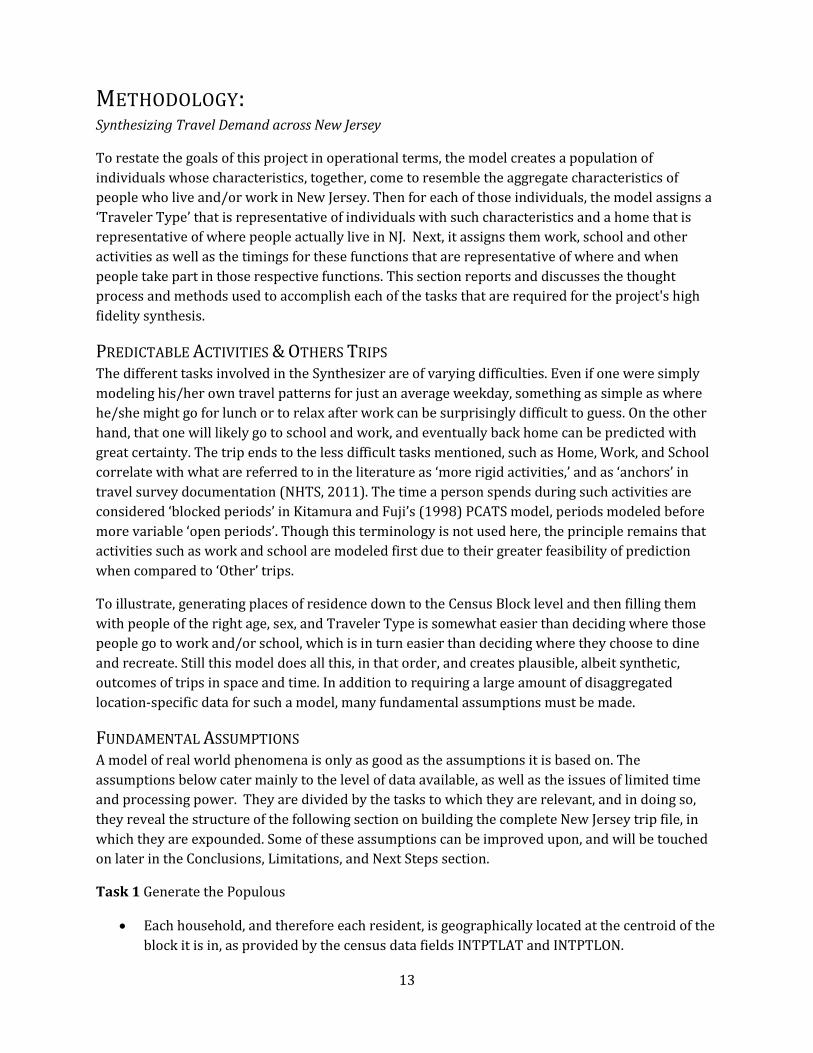
Task 1 Generate the Populous

Each household, and therefore each resident, is geographically located at the centroid of the

block it is in, as provided by the census data fields INTPTLAT and INTPTLON.

14

The number of people by age and sex is known down to the Census Block level, but ages are

divided by the census into intervals, 0-4, 5-9, etc. Ages within these intervals are assumed to

be distributed uniformly and are sampled as such1.

The population is divided into households and group quarters such as dormitories and

nursing homes. All are represented as households however and have a household type from

0 to 8. 0 and 1 refer to actual households and the rest refer to group quarters - a full list is

shown in Table 1 Codes for Traveler Types, Household Types, and Income BracketsTable 1.

Households are built by first choosing a household size and a female or male householder.

The rest are filled based on household relations distributions as in table P29 in the Census

SF1. All sampling used here (and later on) is done with replacement.

Residents are assigned a Traveler Type from 0-7, which helps the Synthesizer categorize

them and later specify their potential sequences of daily activities.

Traveler Type is based on age and household type (particularly if the household is a group

quarter).

Incomes are assigned to each entire household to reflect in aggregate the income

characteristics of each Census Tract. It is then divided among its residents that work to

assign them individual incomes.

Task 2 Assign Work Places

Workers from out of state are generated deterministically from the 2000 Journey to Work

Census data rather than sampled.

Out-of-state workers are given Household and Traveler Types of 9 and 7 respectively and

are immediately assigned a county to work in. Their records are saved in seven different

files based on where they reside.

Every resident worker is first assigned a working county where their employment is located

to reflect in aggregate the county-to-county flow from the 2000 Journey to Work Census

data.

All non-workers like children and the elderly, as well as Homeworkers (Traveler Type 6)—

including homemakers, the unemployed, or even workers on a sick day—are given a -1

instead of a working county.

Workers who work outside the state are assigned a -2 instead of a working county.

Workers who are in school, college, or university work in the same county that they live in

by default.

Workers are then assigned an industry, followed by an employer within that industry. Both

are drawn from distributions built using attraction equations.

Task 3 Assign Schools

Despite the availability of data on preschools and kindergartens that have children under

the age of 5, residents in this age range are of Traveler Type 0 and are not assigned a school,

as their travel patterns are typically tied more to that of their parents.

1 There exist a few blocks so lowly populated that this information is only available at tract level and not displayed at the block level, for privacy concerns.

15

The data detailing the percent of students enrolled by level and age group used here is at

the national level.

The proportion of enrolled students in public and private institutions by age group, school

level, and sex is available at the county level, though age group is used rather than school

level.

For simplicity, lists of schools, colleges, and universities drawn from, both public and

private, are limited to those in the same county as the student.

For public K-12 schools of any level, no sampling is done; rather the school nearest to the

child’s resident Census Block is chosen.

For private schools and higher education, sampling is done with replacement, as has been

the case in previous modules.

Private schools and colleges/universities are sampled from distributions built using an

attraction equation, which is weighted by the size of the school over the squared distance

between campus centroid and centroid of the Census Block the student lives in.

Task 4 Assign Tours/Activity Patterns

All tours begin and end at Home.

Revised Traveler Type is assigned to deal with students (TT’s 1-4) who are assigned as “Not

Enrolled” (Student Type 9). TT’s 1, 2, and 4 are changed to TT 1, Homeworkers. TT 3’s

becomes 5’s as they simply work that day without attending college.

For simplicity, there are exactly 17 different Activity Patterns (referred to in the code as

Tour Types), with a different probability for every type of resident.

If the resident is a Homeworker, all Work nodes in any of the Activity Patterns are

considered Other nodes.

Task 5 Assign Other Trips

Other trips made from work during lunch hours must be within the work county (Type 11)

The rest of the Other trips can be in the county itself or any county that is 1-adjacent to it, or

neighboring.

An O location (place of patronage) is drawn randomly with replacement from a distribution

that is weighted by the daily patronage at the place divided by the L2 (Euclidean) distance

from home to the place, even when it is an Other trip following another Other trip.

Any trip less than the equivalent of a quarter-mile in distance is ignored, and for Other trips

that are followed by a return to work (Type 11), they must be less than 5 miles away or the

next nearest place of patronage.

Task 6 Assign Arrival and Departure Times

Arrival and Departure Times are all represented by asymmetrical triangular distributions

for simplicity, such that few people arrive late or leave early.

All times are in seconds after midnight.

Only one average speed is used for all trips, 30 MPH.

16

All distances here are calculated more precisely using Great Circle Distance (aka Haversine

distance).

Durations of stay at places of patronage are also drawn using a triangular distribution, the

parameters of which are hardcoded to reflect times spent recreating. Minimum is set to 6

minutes, maximum to 2 hours and the mode to 20 minutes.

With the fundamental assumptions of each part of the simulation covered, the following sections

proceed to explain more fully each task and how they come together to produce the final trip file.

Each task is written up in python code as a module, links to which can be found in the appendix on

page 78.

17

TASK 1: GENERATING THE POPULACE The first task operates primarily based on population and household demographics from the 2010

Decennial Census. The goal of Module 1—the programming counterpart to Task 1–is to output a

complete resident file for each county in the state. This resident file can be seen as a synthetically

generated database that includes rows/records for individual people and columns/fields for

particular attributes. These attributes include county number, Household ID, Household Type,

latitude and longitude, ID number, Age, Sex, Traveler Type and Income Bracket.

New Jersey counties are represented by an odd number between 1 and 41 following the FIPS

County codes; though, within the modules’ coding a custom code from 0-20 is sometimes used for

convenience. Out-of-state counties and their categorization into regions are also coded with

numbers following 41 and 20 (FIPS and custom codes respectively) but are not dealt with until

Task 2. Next, an integer household ID, tracks which household the resident is in. Residents in the

same household are displayed in consecutive rows with the same household ID. Household Type

uses an integer from 0 to 8 to describe the kind of household or group quarter as shown in Table 1

below.

The latitude and longitude of the center of population (2010 Census Centers of Population by

County, 2010) of the Census Block which the resident is in are expressed to 7 decimal places. Every

resident's ID starts with a three letter code for the county he/she lives in, followed by an 8 digit

number. Then the age and sex of each resident are added, followed by an integer between 0 and 8

representing Traveler Type. And lastly, a code from 0 to 10 signifies which income bracket the

resident falls under. All integer-represented attributes are detailed in the table below.

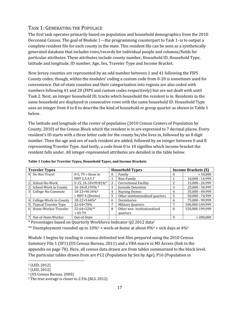
Table 1 Codes for Traveler Types, Household Types, and Income Brackets

Traveler Types Household Types Income Brackets ($) 0 Do-Not-Travel 0-5, 79 + those in

HHT 2,3,4,5,7 0 Family 0 < 10,000 1 Non-Family 1 10,000 - 14,999

1 School-No-Work 5-15, 16-18×99.81%* 2 Correctional Facility 2 15,000 - 24,999 2 School-Work in County 16-18×0.193% * 3 Juvenile Detention 3 25,000 - 34,999 3 College-No-Commute 18-22×90.34%*

+ HHT 6 (Dorms) 4 Nursing Homes 4 35,000 - 49,999 5 Other institutionalized quarters 5 50,000 - 74,999

4 College-Work-in-County 18-22×9.66%* 6 Dormitories 6 75,000 - 99,999 5 Typical Traveler Type 22-64×78% 7 Military Quarters 7 100,000-149,999 6 Home-Worker-Traveler 22-64×22%**

+ 65-79 8 Other noninstitutionalized

quarters 8 150,000-199,999

7 Out-of-State-Worker Out-of-State 9 > 200,000

* Percentages based on Quarterly Workforce Indicator Q2 2012 data2

** Unemployment rounded up to 10%3 + work-at-home at about 8%4 + sick days at 4%5

Module 1 begins by reading in comma-delimited text files prepared using the 2010 Census

Summary File 1 (SF1) (US Census Bureau, 2011) and a VBA macro in MS Access (link in the

appendix on page 78). Here, all census data drawn are from tables summarized to the block level.

The particular tables drawn from are P12 (Population by Sex by Age), P16 (Population in 2 (LED, 2012) 3 (LED, 2012) 4 (US Census Bureau, 2005) 5 The true average is closer to 2.5% (BLS, 2012)

18

Households by Age—the table differentiates by ages under/over 18), P29 (Household Type by

Relationship), H13 (Household Size), and P43 (Group Quarter Population by Sex by Age by Group

Quarter Type). There are likely many ways one could use these and other tables from SF1 to

generate a synthetic population for a state. The method used in Module 1 is repeated for every

Census Block in every county and is explained briefly below in the following paragraphs. In addition

to data from SF1, income data is read in from the 2010 5-Year American Community Survey (US

Census Bureau, 2011). This will be explained further below when describing assigning incomes to

households and residents.

The census makes available exact block-level data stating the number of people for each sex in each

age group (P12). These are iterated through, generating the appropriate number of residents for

each group. Their exact age is then chosen randomly by uniformly sampling from within the

particular age range. These are kept in four lists, male adults, female adults, male children, and

female children, which are shuffled so that they do not remain in the original order of iteration,

youngest to oldest age groups. The cut-off age for children in this model is 22 rather than 18 for

simplicity that will become apparent in Task 3: Assigning Schools and other Educational

Institutionswhere schools and universities are assigned.

Next, the module begins to form households of different sizes and types. It first iterates over a

census data table (H13) which states exactly how many households of sizes 1 to 7+ exist in each

block—in this model 7 is the maximum number of occupants generated for any Non-Group Quarter

household. For each household in each of these household sizes, the program calls a function to

create a single household of the appropriate size. This function works by first selecting whether or

not the household is considered a family (Household Type 0) or non-family (Household Type 1),

since this affects which distribution to use in determining household members. Next it chooses

whether the main householder is a male or a female; again, the distribution sampled from to decide

this differs based on family status. Afterwards the remaining members of the household are chosen

where the main aspects differentiating them are sex and adult/child status. To illustrate this with

an example, two of the fields in table P29 are "Male Biological Child" and "Male Adopted Child,"

however this level of detail is beyond the scope of this model and thus when either of these options

is drawn, the household member created is simply considered a male child. Sampling this way, the

appropriate number of times, creates an empty shell for the household. This is then represented by

a list, which is filled by popping residents, as appropriate, from the male adults, female adults, male

children, and female children lists (here used as stacks) mentioned earlier. Returning to our

example, the male children list would be popped twice thus choosing two male children that were

generated for this Census Block.

With households of types 0 and 1 generated for a Census Block, the model now generates residents

living in other living spaces, which the Census calls Group Quarters. These include places such as

military barracks and school dormitories among others detailed in Table 1 above. Table P43

includes a great level of detail, dividing the population into institutionalized quarters like

correctional and juvenile facilities and noninstitutionalized quarters such as student housing and

military quarters, with those all divided into three age categories: Under 18 years, 18 to 64 years,

and 65 years and over. The model assumes only one of each type of quarter per Census Block. This

follows the reasoning that most such quarters would be rather large in comparison to the area of a

19

single Census Block. The presence of multiple ones is both unlikely and effectively the same for the

purposes of this model. As such, the table is iterated through and group quarters, much like

households are represented by lists which are populated by popping the appropriate types of

residents from their respective lists. In the remainder of this thesis, unless otherwise mentioned,

the term household will also include Group Quarters or Household Types 2 to 8. In populating the

block's group quarters, certain other information can immediately be determined and assigned to

their residents, namely, Traveler Type and Income Bracket, the final two attributes given to each

resident in this model's resident file.

Now every resident is assigned a Traveler Type, numbered from 0 to 6 such as School-No-Work (1)

and Homeworker-Traveler (6). These are based primarily on a resident's age and the type of

household which they reside in. For example, people in adult correctional facilities and those over

65 in nursing facilities are all of Traveler Type, Do-Not-Travel (0). The rest are detailed in Table 1

above based on a distribution that is currently hard-coded to reflect the distribution for the whole

state (see Conclusions, Limitations, and Next Steps for how this could be improved).

20

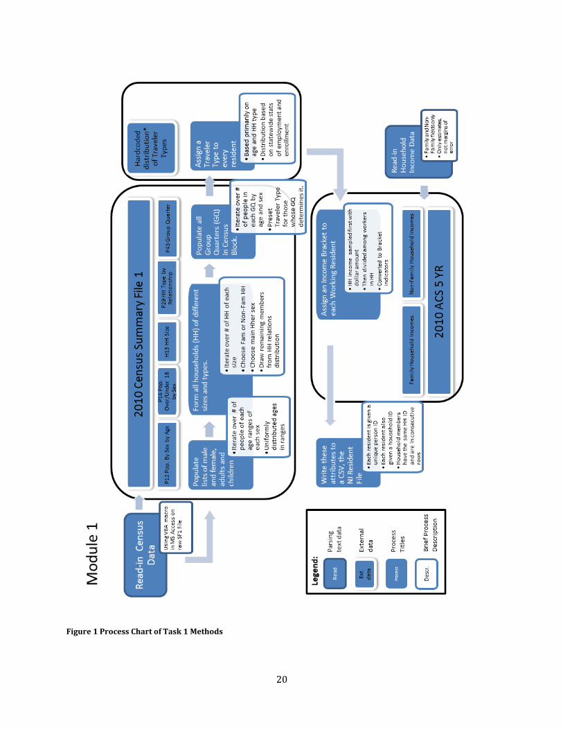
Figure 1 Process Chart of Task 1 Methods

21

Three more Traveler Types are relevant at this time: School-Work-in-County ( 2), College-Work-in-

County( 4), Typical-Traveler-Type ( 5). Residents of these types, as well as Homeworker-Travelers

are all assigned an Income Bracket coded between 1 and 10—0 indicates no income. For the first

three, this is of consequence because it will be used in Module 2 to help choose where that resident

works; not so for type 6 residents because they work at home by definition.

As mentioned earlier, before iterating over the Census Blocks in a county, Census data relevant to

the county are read. Before this, however, household income data are read for the entire state. This

is done because the data are available only at the Census Tract level, thus the file is not nearly as

long. This file can be generated easily using the American FactFinder website (American FactFinder,

2012). It includes the estimated number of households of different types—family and non-family

households are used here—in each income bracket. These estimates are used as distributions from

which Non-Group Quarter household incomes are sampled. The file also includes margins of error

as well as other estimates, however these are never used, and only relevant data are read by the

module.

The data are first sampled for every household to generate a household income; a dollar amount is

randomly drawn uniformly within the range of the income bracket. This is then distributed over all

working members of the household. Once again there are many possible ways in which this could

be done; for example, age and/or position in the household could be taken into consideration. In

this instance, the module uses a simple function which randomly generates a coefficient for each

worker (these coefficients sum to 1), which decides the portion of the household income that

he/she makes annually. Each income is then aggregated to an Income Bracket (from 1 to 10) which

it falls under.

Figure 2 Population Hierarchy

22

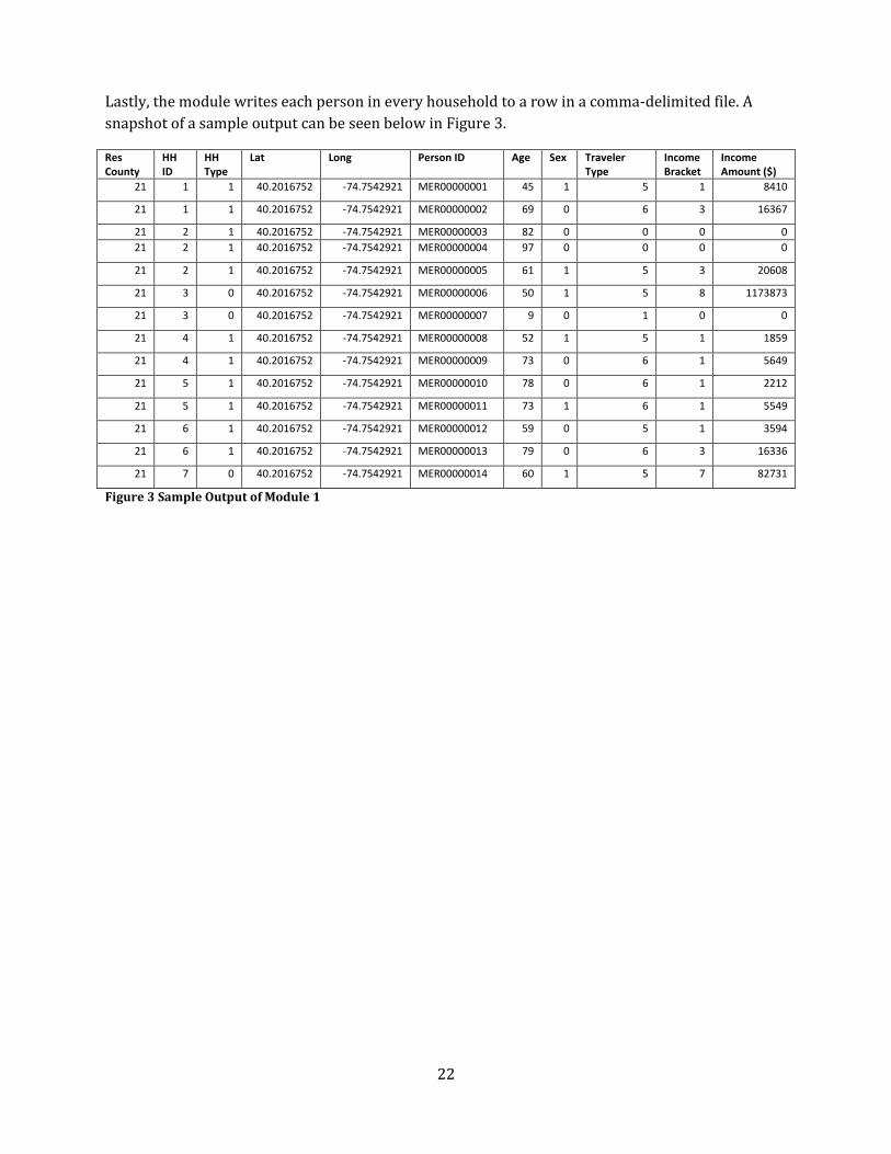
Lastly, the module writes each person in every household to a row in a comma-delimited file. A

snapshot of a sample output can be seen below in Figure 3.

Res County

HH ID

HH Type

Lat Long Person ID Age Sex Traveler Type

Income Bracket

Income Amount ($)

21 1 1 40.2016752 -74.7542921 MER00000001 45 1 5 1 8410

21 1 1 40.2016752 -74.7542921 MER00000002 69 0 6 3 16367

21 2 1 40.2016752 -74.7542921 MER00000003 82 0 0 0 0

21 2 1 40.2016752 -74.7542921 MER00000004 97 0 0 0 0

21 2 1 40.2016752 -74.7542921 MER00000005 61 1 5 3 20608

21 3 0 40.2016752 -74.7542921 MER00000006 50 1 5 8 1173873

21 3 0 40.2016752 -74.7542921 MER00000007 9 0 1 0 0

21 4 1 40.2016752 -74.7542921 MER00000008 52 1 5 1 1859

21 4 1 40.2016752 -74.7542921 MER00000009 73 0 6 1 5649

21 5 1 40.2016752 -74.7542921 MER00000010 78 0 6 1 2212

21 5 1 40.2016752 -74.7542921 MER00000011 73 1 6 1 5549

21 6 1 40.2016752 -74.7542921 MER00000012 59 0 5 1 3594

21 6 1 40.2016752 -74.7542921 MER00000013 79 0 6 3 16336

21 7 0 40.2016752 -74.7542921 MER00000014 60 1 5 7 82731

Figure 3 Sample Output of Module 1

23

TASK 2: ASSIGNING WORK PLACES TO WORKERS The second task generates exact work places for every worker in New Jersey, including both

working residents generated in Task 1 as well as out-of-state workers which commute to different

counties in the state.

First, Module 2a, the first python script used in Task 2, creates seven resident files, identical in

format to those made in Task 1, to account for people who work in New Jersey but reside outside

the state. Those who reside outside the United States and Canada are ignored in our model due to

their relatively low numbers. These workers are all assigned a Traveler Type of 7 and a Household

Type of 9, which reflect that their households are not in the state and that their travel pattern

reflects that only come to NJ for work. They are also given an age uniformly chosen between 22 and

65 and a sex drawn at random with a higher probability, 0.61, of being Male. In any case, these

attributes play no role in choosing their work place or travel patterns within the scope of this

model. In fact, the counties in which each worker lives and works is known deterministically from

the 2000 Journey-to-Work Census data's County to County flows file sorted by work state and

county. This data is only publicly available at the only county level for privacy reasons (US Census

Bureau, 2000).

Figure 4 Process Chart of Task 2 Methods for non-NJ Counties

Nevertheless, since the county which they work in within New Jersey is given, determining the

work county is trivial. As for their residence counties, all locations are categorized into 7 possible

places for the scope of this project, outlined below (credit to N. Webb for its initial compilation).

Table 2 Out-of-State Locations and Categorizations

ID Custom Coding

Ext. FIPS

Region Exact Location Latitude, Longitude

NYC 21 42 New York City Empire State Building (40.748716,-73.986171) PHL 22 43 Philadelphia Ben Franklin statue (39.952335,-75.163789) BUC 23 44 Bucks County PA and West to CA Newtown, PA (40.229275,-74.936833) SOU 24 45 South of Philadelphia Wilmington DE (39.745833,-75.546667) NOR 25 46 North of Bucks County in PA Allentown PA (40.608431,-75.490183) WES 26 47 Westchester County NY and East White Plains (41.033986,-73.76291) ROC 27 48 Rockland, Orange and Rest of NY State Rockland (41.148946,-73.983003) INTL 28 49 Outside the United States NY Penn Station (40.750580,-73.993580)

24

A complete dictionary mapping each state and/or county to one of these locations, is used in all

three parts of Module 2 and are based on work first done by A. Kumar for his part of the ORF467

Trip Synthesizer project Module 2a is essentially a simplified version of Task 1 for out-of-state

workers. Module 2c assigns work related attributes in much the same as shall now described for

the New Jersey residents and will be elaborated on at the end of this section to highlight

noteworthy differences from 2b.

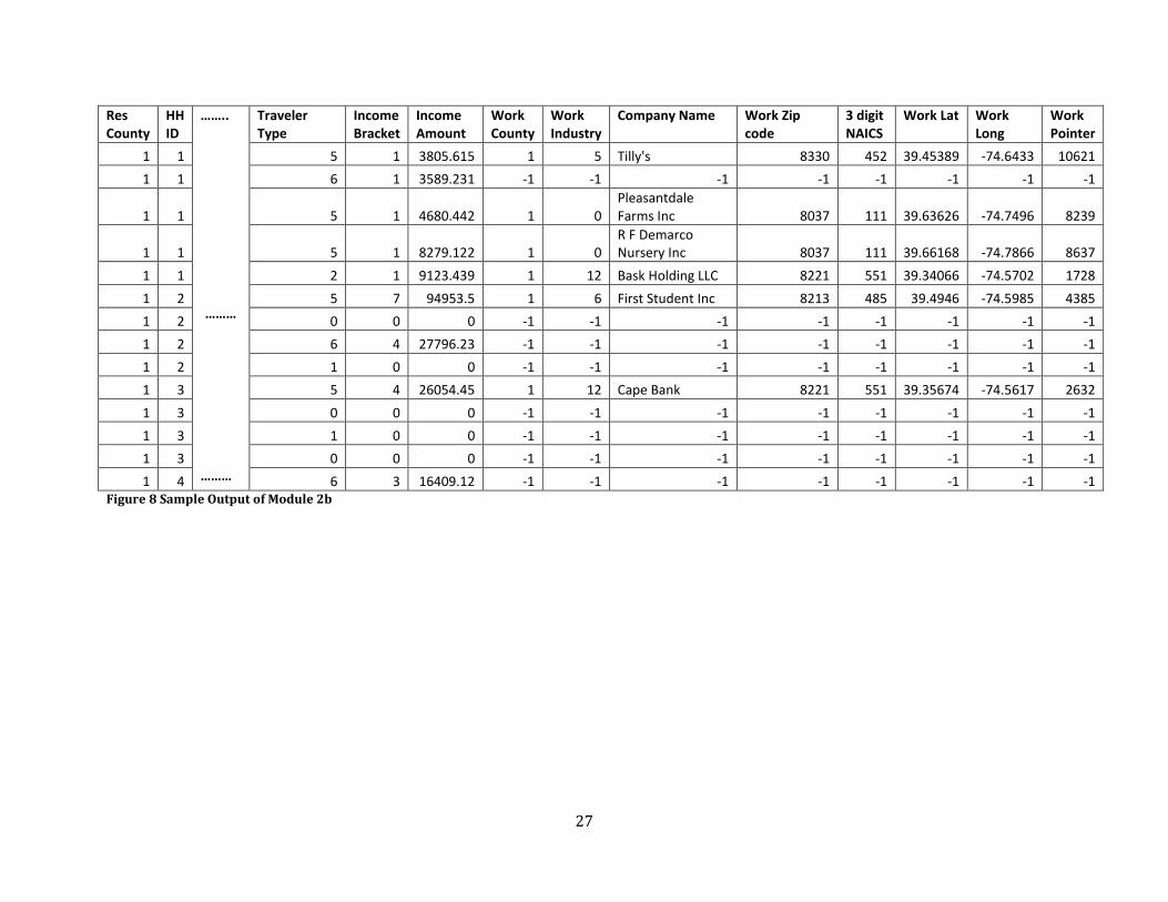
Module 2b, reads in the 21 New Jersey resident files generated in Task 1 so as to append to them

the following fields, Work County, Simplified Industry Code, Company of Employment's Name,

Employment Zip Code, 3-digit NAICS code, a pointer into the work file, Latitude and Longitude. Note

that the pointer, currently, is a row number that refers directly into the Employer file with a header,

as it would be viewed in a spreadsheet editor. Due to indices starting with 0 in the code—but 1 in

say Excel—and the skipping of the header, should the pointer be used for later code, 1 or 2 may

have to be subtracted.

First each resident is assigned an integer to indicate which county they work in, if they work at all.

-1 indicates that they do not work, and odd numbers from 1 to 41 (FIPS county codes) represent the

21 counties in New Jersey, with the out-of-state locations represented by consecutive numbers

following that, 42 – 49, where 49 is International and is not given an exact location. Rather, the

coordinates for international workers are set to those of New York Penn Station. For Traveler Type

5 residents—workers—work counties are drawn from the 2000 Journey-to-Work Census data's

County to County flows file sorted by residence state and county. When a county outside the state is

drawn, one of the seven locations listed above is chosen based on the previously mentioned

mapping (US Census Bureau, 2000).

Table 3 Industry Codes used in Module 2

Code 2-digit Truncated NAICS Name -2 - Out-of-State; No Industry Assigned 0 11 Agriculture Forestry Fishing and Hunting 1 21 Mining 1 22 Utilities 3 23 Construction 4 31 Manufacturing 4 32 Manufacturing 4 33 Manufacturing 5 42 Wholesale Trade 6 44 Retail Trade 6 45 Retail Trade 7 48 Transportation and Warehousing 7 49 Transportation and Warehousing 8 51 Information 9 52 Finance and Insurance 10 53 Real Estate and Rental and Leasing 11 54 Professional Scientific and Technical Services 12 55 Management of Companies and Enterprises 13 56 Administrative and Support and Waste Management and Remediation Services 14 61 Education Services 15 62 Health Care and Social Assistance

25

16 71 Arts Entertainment and Recreation 17 72 Accommodation and Food Services 18 81 Other Services 19 92 Public Administration

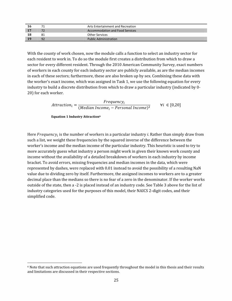
With the county of work chosen, now the module calls a function to select an industry sector for

each resident to work in. To do so the module first creates a distribution from which to draw a

sector for every different resident. Through the 2010 American Community Survey, exact numbers

of workers in each county for each industry sector are publicly available, as are the median incomes

in each of these sectors; furthermore, these are also broken up by sex. Combining these data with

the worker's exact income, which was assigned in Task 1, we use the following equation for every

industry to build a discrete distribution from which to draw a particular industry (indicated by 0-

20) for each worker.

( )

Equation 1 Industry Attraction6

Here is the number of workers in a particular industry i. Rather than simply draw from

such a list, we weight these frequencies by the squared inverse of the difference between the

worker’s income and the median income of the particular industry. This heuristic is used to try to

more accurately guess what industry a person might work in given their known work county and

income without the availability of a detailed breakdown of workers in each industry by income

bracket. To avoid errors, missing frequencies and median incomes in the data, which were

represented by dashes, were replaced with 0.01 instead to avoid the possibility of a resulting NaN

value due to dividing zero by itself. Furthermore, the assigned incomes to workers are to a greater

decimal place than the medians so there is no fear of a zero in the denominator. If the worker works

outside of the state, then a -2 is placed instead of an industry code. See Table 3 above for the list of

industry categories used for the purposes of this model, their NAICS 2-digit codes, and their

simplified code.

6 Note that such attraction equations are used frequently throughout the model in this thesis and their results and limitations are discussed in their respective sections.

26

Figure 5 Process Chart of Task 2 Methods for NJ

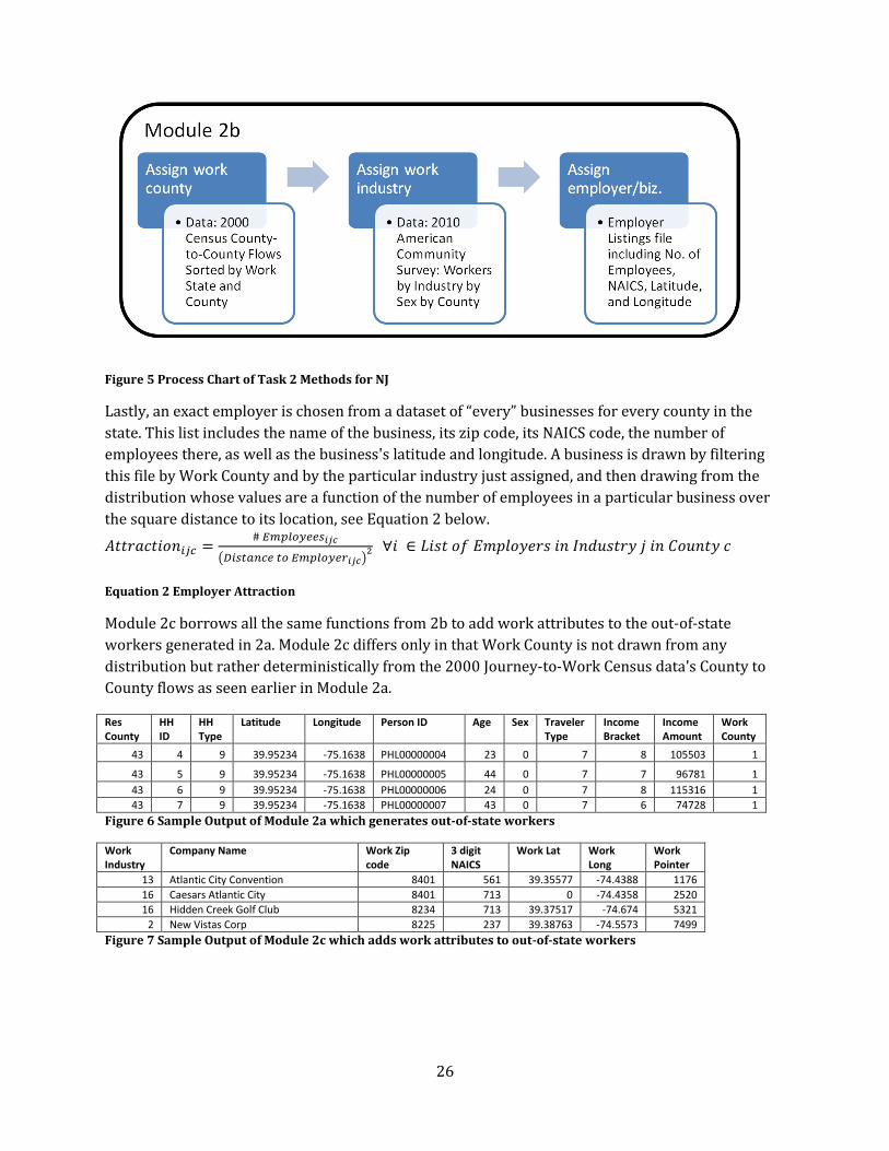
Lastly, an exact employer is chosen from a dataset of “every” businesses for every county in the

state. This list includes the name of the business, its zip code, its NAICS code, the number of

employees there, as well as the business's latitude and longitude. A business is drawn by filtering

this file by Work County and by the particular industry just assigned, and then drawing from the

distribution whose values are a function of the number of employees in a particular business over

the square distance to its location, see Equation 2 below.

( )

Equation 2 Employer Attraction

Module 2c borrows all the same functions from 2b to add work attributes to the out-of-state

workers generated in 2a. Module 2c differs only in that Work County is not drawn from any

distribution but rather deterministically from the 2000 Journey-to-Work Census data's County to

County flows as seen earlier in Module 2a.

Res County

HH ID

HH Type

Latitude Longitude Person ID Age Sex Traveler Type

Income Bracket

Income Amount

Work County

43 4 9 39.95234 -75.1638 PHL00000004 23 0 7 8 105503 1

43 5 9 39.95234 -75.1638 PHL00000005 44 0 7 7 96781 1

43 6 9 39.95234 -75.1638 PHL00000006 24 0 7 8 115316 1

43 7 9 39.95234 -75.1638 PHL00000007 43 0 7 6 74728 1

Figure 6 Sample Output of Module 2a which generates out-of-state workers

Work Industry

Company Name Work Zip code

3 digit NAICS

Work Lat Work Long

Work Pointer

13 Atlantic City Convention 8401 561 39.35577 -74.4388 1176

16 Caesars Atlantic City 8401 713 0 -74.4358 2520

16 Hidden Creek Golf Club 8234 713 39.37517 -74.674 5321

2 New Vistas Corp 8225 237 39.38763 -74.5573 7499

Figure 7 Sample Output of Module 2c which adds work attributes to out-of-state workers

27

Res County

HH ID

…….. ………

………

Traveler Type

Income Bracket

Income Amount

Work County

Work Industry

Company Name Work Zip code

3 digit NAICS

Work Lat Work Long

Work Pointer

1 1 5 1 3805.615 1 5 Tilly's 8330 452 39.45389 -74.6433 10621

1 1 6 1 3589.231 -1 -1 -1 -1 -1 -1 -1 -1

1 1 5 1 4680.442 1 0 Pleasantdale Farms Inc 8037 111 39.63626 -74.7496 8239

1 1 5 1 8279.122 1 0 R F Demarco Nursery Inc 8037 111 39.66168 -74.7866 8637

1 1 2 1 9123.439 1 12 Bask Holding LLC 8221 551 39.34066 -74.5702 1728

1 2 5 7 94953.5 1 6 First Student Inc 8213 485 39.4946 -74.5985 4385

1 2 0 0 0 -1 -1 -1 -1 -1 -1 -1 -1

1 2 6 4 27796.23 -1 -1 -1 -1 -1 -1 -1 -1

1 2 1 0 0 -1 -1 -1 -1 -1 -1 -1 -1

1 3 5 4 26054.45 1 12 Cape Bank 8221 551 39.35674 -74.5617 2632

1 3 0 0 0 -1 -1 -1 -1 -1 -1 -1 -1

1 3 1 0 0 -1 -1 -1 -1 -1 -1 -1 -1

1 3 0 0 0 -1 -1 -1 -1 -1 -1 -1 -1

1 4 6 3 16409.12 -1 -1 -1 -1 -1 -1 -1 -1 Figure 8 Sample Output of Module 2b

28

TASK 3: ASSIGNING SCHOOLS AND OTHER EDUCATIONAL INSTITUTIONS The third task deals with assigning a place of study to residents designated Traveler Types 1

through 4, namely students in K-12 schools, colleges, universities and other schools such ones for

the severely handicapped.

To begin the module looks at each resident and assesses whether they are special needs students or

not. Though a relatively large number of public school students qualify as "Special Needs," the

number of students that attend a dedicated school for handicapped children is about l0,660, or 0.66

% of all K-12 students, according to the New Jersey Department of Education. A randomly drawn

number between 0 and 1 is drawn and compared to this figure to decide whether the student in

question should be assigned a Student Type of 6.

The module then decides whether or not they are enrolled in any non-special school and which

level of education their schooling falls under, and whether that school is private or public. The

datasets from which these attributes are drawn are detailed in the Data section under School Data

Sets. A function performs these checks in that order and assigns one of the following Student Types

to each resident:

0 – Public Elementary School

1 – Public Middle School

2 – Public High School

3 – Private Elementary School

4 – Private Middle School

5 – Private High School

6 – Special Needs

7 – Commuter College/University

8 – Non-commuter College/University

9 – Not Enrolled

Figure 9 Process Chart of Task 3 Methods

29

Next, the resident's Household Type is checked. The assumption is made that residents in Group

Quarters other than dormitories don't go to school or college for simplicity, though in reality a small

number of juvenile detentions do allow children to go to school. Residents in dormitories

(Household Type 6) are automatically assigned a School Type of 8, Non-commuter

College/University. For Household Types of 0 or 1, more typical family or non-family residences,

the enrollment distribution data and private versus public distribution data mentioned earlier are

drawn from, based on age and county, to determine whether the student goes to, say, public middle

school, private high school, or is perhaps not enrolled at all.

With a Student Type assigned to the resident in question, the module goes on to choose an exact

school or educational institution which the resident goes to on a typical weekday morning. In its

current build, the module reads from six files, each of which includes at least School Name, Position

(latitude and longitude), and Total Student Enrollment. In the previous iteration of this project done

by the class of ORF 467 Fall ’11, a separate file was used for each of the student types (other than 9)

resulting in 8 files. While public school data and college/university data were readily accessible

from the website of the New Jersey Department of Education, private school data were poorly

fabricated due to difficulty locating enrollment data at the time. Further research led to finding

these data at the National Center of Education Statistics Website which performs a yearly survey of

private schools across the nation. As such all private school data are currently in one file, bringing

the number of school enrollment files to 6.

Different methods were used to pick different types of institutions. Public K-12 schools and Special

schools were picked purely by shortest great circle distance from schools to the household; both in

the same county. This assumption isn’t unreasonable as School Districts never cross County

boundaries. The mapping is not one-to-one, however. Multiple districts do sometimes exist in the

same County. Ostensibly, a mapping of Census Blocks to School Districts should be simple to make

and use. However, when attempted using the SF1 data, the districts simply did not match those in

the school file (which are most likely the correct ones); so, distance was used instead. Furthermore,

to save time on repeated calculations, these distances could have been calculated only once per

Census Block, however due to the relatively small number of public schools of each level within a

single county, they are calculated every time for different students. One advantage of this, however,

is that in future renditions where each household may be given a location different from and more

accurate than just the Census Block centroid, the code for choosing public schools would still work.

Private schools and all places of higher education are picked randomly from a distribution whose

values are produced by a function of student enrollment (i.e. school size) and distance, much like

the attraction equation used to select industries as a function of frequency and income difference. It

is as follows in Equation 3 for every college/university and private K-12 school.

( ( ))

Equation 3 Private School Attraction

30

Here GCD refers to Great Circle distance, a method of calculating distance between two points on a

sphere; in this case using latitude and longitude coordinates and assuming the Earth’s radius to be

3963.17 miles to cater to coordinates in the Northeast of America.

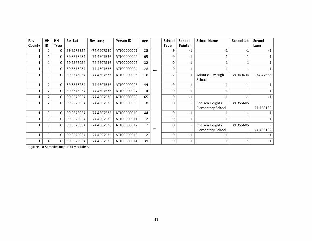
Once an institution is picked for every enrolled student, a new Task 3 file is created for every

county relisting all information from the previous two tasks and appending school information,

specifically Student Type, School Name, a pointer into the school file(i.e. a row number), and the

school's Latitude and Longitude coordinates. Sample output can be found in Figure 10 below.

31

Res County

HH ID

HH Type

Res Lat Res Long Person ID Age ….. ….

School Type

School Pointer

School Name School Lat School Long

1 1 0 39.3578934 -74.4607536 ATL00000001 28 9 -1 -1 -1 -1

1 1 0 39.3578934 -74.4607536 ATL00000002 69 9 -1 -1 -1 -1

1 1 0 39.3578934 -74.4607536 ATL00000003 32 9 -1 -1 -1 -1

1 1 0 39.3578934 -74.4607536 ATL00000004 28 9 -1 -1 -1 -1

1 1 0 39.3578934 -74.4607536 ATL00000005 16 2 1 Atlantic City High School

39.369436 -74.47558

1 2 0 39.3578934 -74.4607536 ATL00000006 44 9 -1 -1 -1 -1

1 2 0 39.3578934 -74.4607536 ATL00000007 4 9 -1 -1 -1 -1

1 2 0 39.3578934 -74.4607536 ATL00000008 65 9 -1 -1 -1 -1

1 2 0 39.3578934 -74.4607536 ATL00000009 8 0 5 Chelsea Heights Elementary School

39.355605 -74.463162

1 3 0 39.3578934 -74.4607536 ATL00000010 44 9 -1 -1 -1 -1

1 3 0 39.3578934 -74.4607536 ATL00000011 2 9 -1 -1 -1 -1

1 3 0 39.3578934 -74.4607536 ATL00000012 7 0 5 Chelsea Heights Elementary School

39.355605 -74.463162

1 3 0 39.3578934 -74.4607536 ATL00000013 2 9 -1 -1 -1 -1

1 4 0 39.3578934 -74.4607536 ATL00000014 39 9 -1 -1 -1 -1

Figure 10 Sample Output of Module 3

32

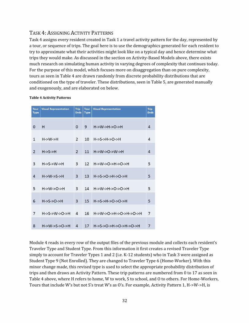
TASK 4: ASSIGNING ACTIVITY PATTERNS Task 4 assigns every resident created in Task 1 a travel activity pattern for the day, represented by

a tour, or sequence of trips. The goal here is to use the demographics generated for each resident to

try to approximate what their activities might look like on a typical day and hence determine what

trips they would make. As discussed in the section on Activity-Based Models above, there exists

much research on simulating human activity in varying degrees of complexity that continues today.

For the purpose of this model, which focuses more on disaggregation than on pure complexity,

tours as seen in Table 4 are drawn randomly from discrete probability distributions that are

conditioned on the type of traveler. These distributions, seen in Table 5, are generated manually

and exogenously, and are elaborated on below.

Table 4 Activity Patterns

Module 4 reads in every row of the output files of the previous module and collects each resident’s

Traveler Type and Student Type. From this information it first creates a revised Traveler Type

simply to account for Traveler Types 1 and 2 (i.e. K-12 students) who in Task 3 were assigned as

Student Type 9 (Not Enrolled). They are changed to Traveler Type 6 (Home-Worker). With this

minor change made, this revised type is used to select the appropriate probability distribution of

trips and then draws an Activity Pattern. These trip patterns are numbered from 0 to 17 as seen in

Table 4 above, where H refers to home, W to work, S to school, and O to others. For Home-Workers,

Tours that include W’s but not S’s treat W’s as O’s. For example, Activity Pattern 1, H->W->H, is

33

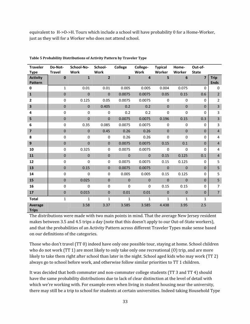
equivalent to H->O->H. Tours which include a school will have probability 0 for a Home-Worker,

just as they will for a Worker who does not attend school.

Table 5 Probability Distributions of Activity Pattern by Traveler Type

Traveler Type

Do-Not-Travel

School-No-Work

School-Work

College College-Work

Typical Worker

Home-Worker

Out-of-State

Activity Pattern

0 1 2 3 4 5 6 7 Trip Ends

0 1 0.01 0.01 0.005 0.005 0.004 0.075 0 0

1 0 0 0 0.0075 0.0075 0.05 0.15 0.6 2

2 0 0.125 0.05 0.0075 0.0075 0 0 0 2

3 0 0 0.405 0.2 0.2 0 0 0 3

4 0 0 0 0.2 0.2 0 0 0 3

5 0 0 0 0.0075 0.0075 0.196 0.15 0.3 3

6 0 0.35 0.085 0.0075 0.0075 0 0 0 3

7 0 0 0.45 0.26 0.26 0 0 0 4

8 0 0 0 0.26 0.26 0 0 0 4

9 0 0 0 0.0075 0.0075 0.15 0.1 0 4

10 0 0.325 0 0.0075 0.0075 0 0 0 4

11 0 0 0 0 0 0.15 0.125 0.1 4

12 0 0 0 0.0075 0.0075 0.15 0.125 0 5

13 0 0.15 0 0.0075 0.0075 0 0 0 5

14 0 0 0 0.005 0.005 0.15 0.125 0 5

15 0 0.025 0 0 0 0 0 0 5

16 0 0 0 0 0 0.15 0.15 0 7

17 0 0.015 0 0.01 0.01 0 0 0 7

Total 1 1 1 1 1 1 1 1

Average Trips

3.58 3.37 3.585 3.585 4.438 3.95 2.5

The distributions were made with two main points in mind. That the average New Jersey resident

makes between 3.5 and 4.5 trips a day (note that this doesn’t apply to our Out-of-State workers),

and that the probabilities of an Activity Pattern across different Traveler Types make sense based

on our definitions of the categories.

Those who don’t travel (TT 0) indeed have only one possible tour, staying at home. School children

who do not work (TT 1) are most likely to only take only one recreational (O) trip, and are more

likely to take them right after school than later in the night. School aged kids who may work (TT 2)

always go to school before work, and otherwise follow similar priorities to TT 1 children.

It was decided that both commuter and non-commuter college students (TT 3 and TT 4) should

have the same probability distributions due to lack of clear distinction at the level of detail with

which we’re working with. For example even when living in student housing near the university,

there may still be a trip to school for students at certain universities. Indeed taking Household Type

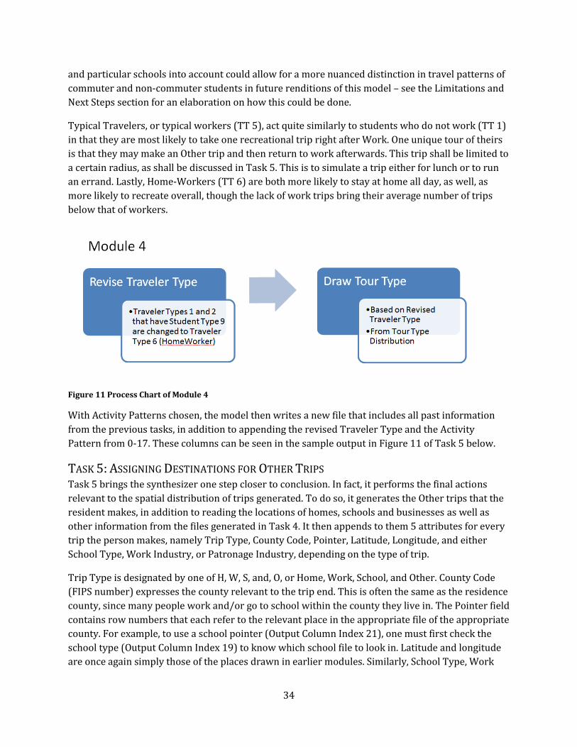
34

and particular schools into account could allow for a more nuanced distinction in travel patterns of

commuter and non-commuter students in future renditions of this model – see the Limitations and

Next Steps section for an elaboration on how this could be done.

Typical Travelers, or typical workers (TT 5), act quite similarly to students who do not work (TT 1)

in that they are most likely to take one recreational trip right after Work. One unique tour of theirs

is that they may make an Other trip and then return to work afterwards. This trip shall be limited to

a certain radius, as shall be discussed in Task 5. This is to simulate a trip either for lunch or to run

an errand. Lastly, Home-Workers (TT 6) are both more likely to stay at home all day, as well, as

more likely to recreate overall, though the lack of work trips bring their average number of trips

below that of workers.

Figure 11 Process Chart of Module 4

With Activity Patterns chosen, the model then writes a new file that includes all past information

from the previous tasks, in addition to appending the revised Traveler Type and the Activity

Pattern from 0-17. These columns can be seen in the sample output in Figure 11 of Task 5 below.

TASK 5: ASSIGNING DESTINATIONS FOR OTHER TRIPS Task 5 brings the synthesizer one step closer to conclusion. In fact, it performs the final actions

relevant to the spatial distribution of trips generated. To do so, it generates the Other trips that the

resident makes, in addition to reading the locations of homes, schools and businesses as well as

other information from the files generated in Task 4. It then appends to them 5 attributes for every

trip the person makes, namely Trip Type, County Code, Pointer, Latitude, Longitude, and either

School Type, Work Industry, or Patronage Industry, depending on the type of trip.

Trip Type is designated by one of H, W, S, and, O, or Home, Work, School, and Other. County Code

(FIPS number) expresses the county relevant to the trip end. This is often the same as the residence

county, since many people work and/or go to school within the county they live in. The Pointer field

contains row numbers that each refer to the relevant place in the appropriate file of the appropriate

county. For example, to use a school pointer (Output Column Index 21), one must first check the

school type (Output Column Index 19) to know which school file to look in. Latitude and longitude

are once again simply those of the places drawn in earlier modules. Similarly, School Type, Work

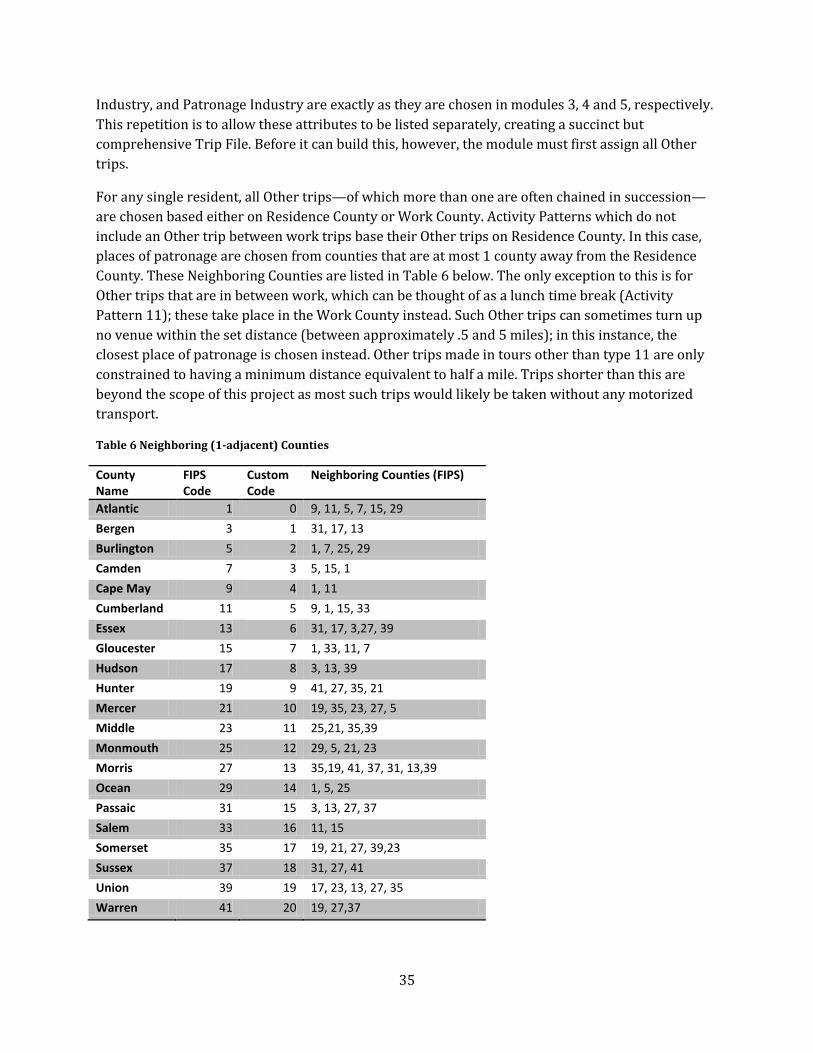
35

Industry, and Patronage Industry are exactly as they are chosen in modules 3, 4 and 5, respectively.

This repetition is to allow these attributes to be listed separately, creating a succinct but

comprehensive Trip File. Before it can build this, however, the module must first assign all Other

trips.

For any single resident, all Other trips—of which more than one are often chained in succession—

are chosen based either on Residence County or Work County. Activity Patterns which do not

include an Other trip between work trips base their Other trips on Residence County. In this case,

places of patronage are chosen from counties that are at most 1 county away from the Residence

County. These Neighboring Counties are listed in Table 6 below. The only exception to this is for

Other trips that are in between work, which can be thought of as a lunch time break (Activity

Pattern 11); these take place in the Work County instead. Such Other trips can sometimes turn up

no venue within the set distance (between approximately .5 and 5 miles); in this instance, the

closest place of patronage is chosen instead. Other trips made in tours other than type 11 are only

constrained to having a minimum distance equivalent to half a mile. Trips shorter than this are

beyond the scope of this project as most such trips would likely be taken without any motorized

transport.

Table 6 Neighboring (1-adjacent) Counties

County Name

FIPS Code

Custom Code

Neighboring Counties (FIPS)

Atlantic 1 0 9, 11, 5, 7, 15, 29

Bergen 3 1 31, 17, 13

Burlington 5 2 1, 7, 25, 29

Camden 7 3 5, 15, 1

Cape May 9 4 1, 11

Cumberland 11 5 9, 1, 15, 33

Essex 13 6 31, 17, 3,27, 39

Gloucester 15 7 1, 33, 11, 7

Hudson 17 8 3, 13, 39

Hunter 19 9 41, 27, 35, 21

Mercer 21 10 19, 35, 23, 27, 5

Middle 23 11 25,21, 35,39

Monmouth 25 12 29, 5, 21, 23

Morris 27 13 35,19, 41, 37, 31, 13,39

Ocean 29 14 1, 5, 25

Passaic 31 15 3, 13, 27, 37

Salem 33 16 11, 15

Somerset 35 17 19, 21, 27, 39,23

Sussex 37 18 31, 27, 41

Union 39 19 17, 23, 13, 27, 35

Warren 41 20 19, 27,37

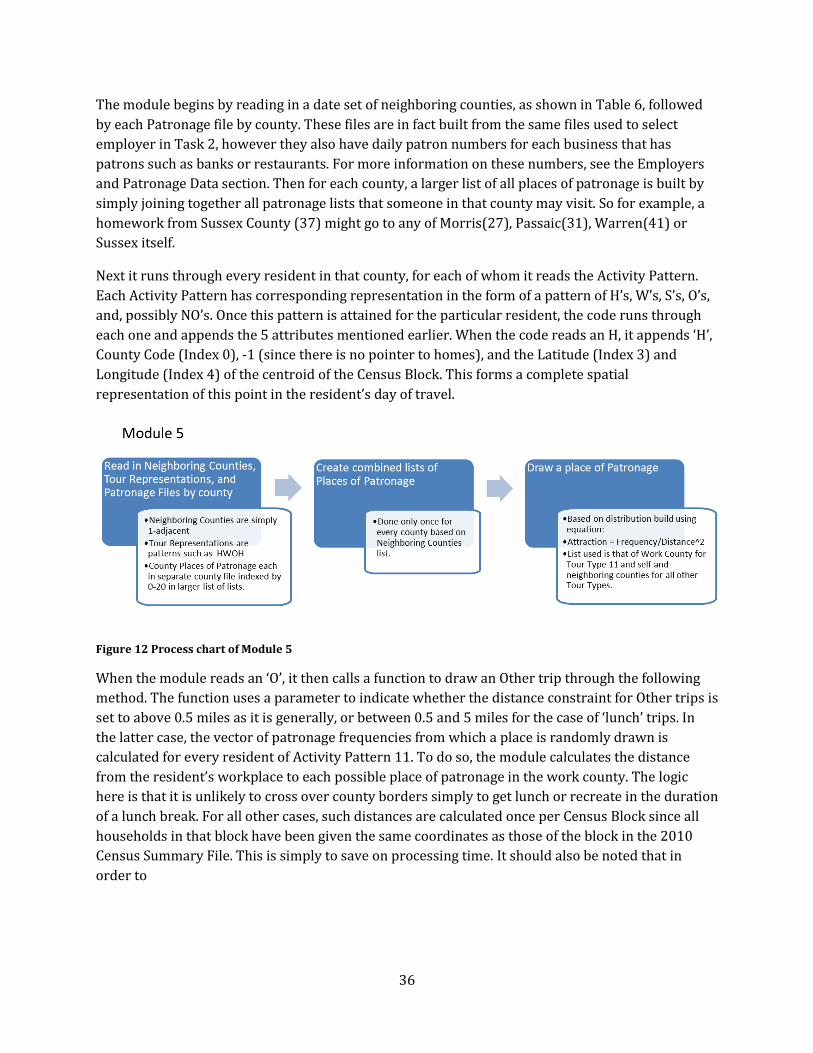
36

The module begins by reading in a date set of neighboring counties, as shown in Table 6, followed

by each Patronage file by county. These files are in fact built from the same files used to select

employer in Task 2, however they also have daily patron numbers for each business that has

patrons such as banks or restaurants. For more information on these numbers, see the Employers

and Patronage Data section. Then for each county, a larger list of all places of patronage is built by

simply joining together all patronage lists that someone in that county may visit. So for example, a

homework from Sussex County (37) might go to any of Morris(27), Passaic(31), Warren(41) or

Sussex itself.

Next it runs through every resident in that county, for each of whom it reads the Activity Pattern.

Each Activity Pattern has corresponding representation in the form of a pattern of H’s, W’s, S’s, O’s,

and, possibly NO’s. Once this pattern is attained for the particular resident, the code runs through

each one and appends the 5 attributes mentioned earlier. When the code reads an H, it appends ‘H’,

County Code (Index 0), -1 (since there is no pointer to homes), and the Latitude (Index 3) and

Longitude (Index 4) of the centroid of the Census Block. This forms a complete spatial

representation of this point in the resident’s day of travel.

Figure 12 Process chart of Module 5

When the module reads an ‘O’, it then calls a function to draw an Other trip through the following

method. The function uses a parameter to indicate whether the distance constraint for Other trips is

set to above 0.5 miles as it is generally, or between 0.5 and 5 miles for the case of ‘lunch’ trips. In

the latter case, the vector of patronage frequencies from which a place is randomly drawn is

calculated for every resident of Activity Pattern 11. To do so, the module calculates the distance

from the resident’s workplace to each possible place of patronage in the work county. The logic

here is that it is unlikely to cross over county borders simply to get lunch or recreate in the duration

of a lunch break. For all other cases, such distances are calculated once per Census Block since all

households in that block have been given the same coordinates as those of the block in the 2010

Census Summary File. This is simply to save on processing time. It should also be noted that in

order to

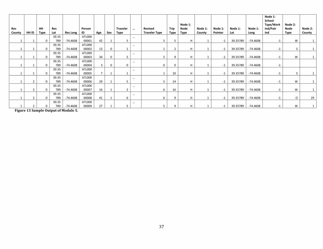
37

Res County HH ID

HH Type

Res Lat Res Long

Person ID Age Sex

Traveler Type

… Revised

Traveler Type Trip Type

Node 1: Node Type

Node 1: County

Node 1: Pointer

Node 1: Lat

Node 1: Long

Node 1: School Type/Work Ind/Patr Ind

Node 2: Node Type

Node 2: County

1 1 0 39.35

789 -74.4608 ATL000

00001 42 1 5 …

5 5 H 1 -1 39.35789 -74.4608 -1 W 1

1 1 0 39.35

789 -74.4608 ATL000

00002 13 0 1 …

1 2 H 1 -1 39.35789 -74.4608 -1 S 1

1 1 0 39.35

789 -74.4608 ATL000

00003 34 0 5 …

5 9 H 1 -1 39.35789 -74.4608 -1 W 1

1 1 0 39.35

789 -74.4608 ATL000

00004 3 0 0 …

0 0 H 1 -1 39.35789 -74.4608 -1

1 1 0 39.35

789 -74.4608 ATL000

00005 7 1 1 …

1 10 H 1 -1 39.35789 -74.4608 -1 S 1

1 2 0 39.35

789 -74.4608 ATL000

00006 29 1 5 …

5 14 H 1 -1 39.35789 -74.4608 -1 W 1

1 2 0 39.35

789 -74.4608 ATL000

00007 16 1 2 …

6 16 H 1 -1 39.35789 -74.4608 -1 W 1

1 2 0 39.35

789 -74.4608 ATL000

00008 41 1 6 …

6 9 H 1 -1 39.35789 -74.4608 -1 O 29

1 2 0 39.35

789 -74.4608 ATL000

00009 27 1 5 …

5 9 H 1 -1 39.35789 -74.4608 -1 W 1

Figure 13 Sample Output of Module 5.

38

reduce processing time, Euclidean L2 distance was used, rather than Great Circle Distance. For the

purposes of using distance as a mere weight to create a distribution from, this is more than

adequate, considering the relatively small range that the coordinates are spread over.

With distances and patronage frequencies available, the module draws from a distribution created

in the following way.

( ( ))

Equation 4 Patronage Attraction

This is repeated until each letter in the resident’s trip chain is read and the row of the resident’s

information is appended with the results of the module, Trip Type, County, Pointer, Latitude,

Longitude, and Industry/School Type for each trip, for each tour, for each resident, for each county.

A few row of abridged sample output are displayed above in Figure 11, which also shows Revised

Traveler Type and Trip Type fields that were added in Module 4.

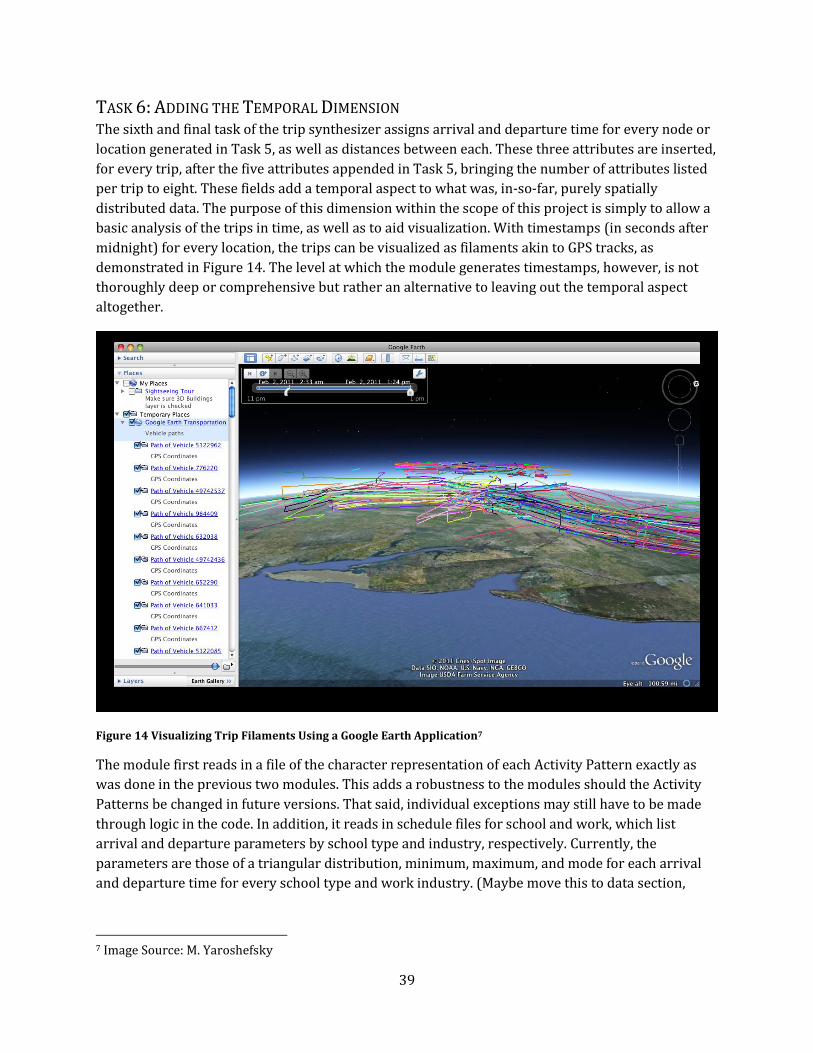
39

TASK 6: ADDING THE TEMPORAL DIMENSION The sixth and final task of the trip synthesizer assigns arrival and departure time for every node or

location generated in Task 5, as well as distances between each. These three attributes are inserted,

for every trip, after the five attributes appended in Task 5, bringing the number of attributes listed

per trip to eight. These fields add a temporal aspect to what was, in-so-far, purely spatially

distributed data. The purpose of this dimension within the scope of this project is simply to allow a

basic analysis of the trips in time, as well as to aid visualization. With timestamps (in seconds after

midnight) for every location, the trips can be visualized as filaments akin to GPS tracks, as

demonstrated in Figure 14. The level at which the module generates timestamps, however, is not

thoroughly deep or comprehensive but rather an alternative to leaving out the temporal aspect

altogether.

Figure 14 Visualizing Trip Filaments Using a Google Earth Application7

The module first reads in a file of the character representation of each Activity Pattern exactly as

was done in the previous two modules. This adds a robustness to the modules should the Activity

Patterns be changed in future versions. That said, individual exceptions may still have to be made

through logic in the code. In addition, it reads in schedule files for school and work, which list

arrival and departure parameters by school type and industry, respectively. Currently, the

parameters are those of a triangular distribution, minimum, maximum, and mode for each arrival

and departure time for every school type and work industry. (Maybe move this to data section,

7 Image Source: M. Yaroshefsky

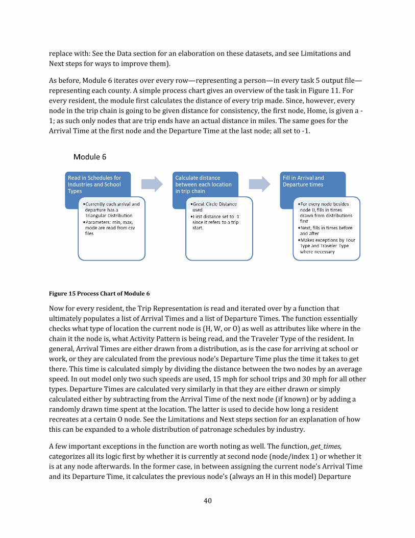
40

replace with: See the Data section for an elaboration on these datasets, and see Limitations and

Next steps for ways to improve them).

As before, Module 6 iterates over every row—representing a person—in every task 5 output file—

representing each county. A simple process chart gives an overview of the task in Figure 11. For

every resident, the module first calculates the distance of every trip made. Since, however, every

node in the trip chain is going to be given distance for consistency, the first node, Home, is given a -

1; as such only nodes that are trip ends have an actual distance in miles. The same goes for the

Arrival Time at the first node and the Departure Time at the last node; all set to -1.

Figure 15 Process Chart of Module 6

Now for every resident, the Trip Representation is read and iterated over by a function that

ultimately populates a list of Arrival Times and a list of Departure Times. The function essentially

checks what type of location the current node is (H, W, or O) as well as attributes like where in the

chain it the node is, what Activity Pattern is being read, and the Traveler Type of the resident. In

general, Arrival Times are either drawn from a distribution, as is the case for arriving at school or

work, or they are calculated from the previous node’s Departure Time plus the time it takes to get

there. This time is calculated simply by dividing the distance between the two nodes by an average

speed. In out model only two such speeds are used, 15 mph for school trips and 30 mph for all other

types. Departure Times are calculated very similarly in that they are either drawn or simply

calculated either by subtracting from the Arrival Time of the next node (if known) or by adding a

randomly drawn time spent at the location. The latter is used to decide how long a resident

recreates at a certain O node. See the Limitations and Next steps section for an explanation of how

this can be expanded to a whole distribution of patronage schedules by industry.

A few important exceptions in the function are worth noting as well. The function, get_times,

categorizes all its logic first by whether it is currently at second node (node/index 1) or whether it

is at any node afterwards. In the former case, in between assigning the current node’s Arrival Time

and its Departure Time, it calculates the previous node’s (always an H in this model) Departure

41

Time by subtracting trip time, in the manner mentioned above. Arrival Time and Distance for the

first node (node/index 0) are set to -1. Similarly, the Departure Time of the final node, also an H, is

set to -1.

After node 1, another exception must be made for tours where the resident both works and goes to

school, or vice versa. This is due to there not being a schedule for those who work and go to school.

To make up for the current simplification, the function shortens both events and ensures that the

second never begins before the first and so on.

With these Arrival Times, Departure Times, and Distances inserted in to each row in the

appropriate trip columns, Module 6 outputs these rows to the final products of this trip synthesizer.

Instead of a sample of this output a clear table of all output fields, their indices, and the module that

generates them is listed below in Table 7.

Table 7 Output Fields by Module ordered by Field Index. Note that Module 6 inserts new fields rather than appending them.

Module Field Index Module Field Index

Module 1 Residence County 0 Module 6 Node 2: Arrival Time 51

HH ID 1 Node 2: Departure Time 52

HH Type 2 Node 2: Distance 53

Residence Latitude 3 Module 5 Node 3: Node Type 54

Residence Longitude 4 Node 3: County 55

Person ID 5 Node 3: Pointer 56

Age 6 Node 3: Latitude 57

Sex 7 Node 3: Longitude 58

Traveler Type 8 Node 3: School Type/Work Industry/Patronage Industry

59

Income Bracket 9 Module 6 Node 3: Arrival Time 60

Income 10 Node 3: Departure Time 61

Module 2 Work County 11 Node 3: Distance 62

Work Industry 12 Module 5 Node 4: Node Type 63

Company Name 13 Node 4: County 64

Work Zip code 14 Node 4: Pointer 65

3 digit NAICS 15 Node 4: Latitude 66

Work Latitude 16 Node 4: Longitude 67

Work Longitude 17 Node 4: School Type/Work Industry/Patronage Industry

68

Work Pointer 18 Module 6 Node 4: Arrival Time 69

Module 3 Student Type 19 Node 4: Departure Time 70

School County 20 Node 4: Distance 71

School Pointer 21 Module 5 Node 5: Node Type 72

School Name 22 Node 5: County 73

School Lat 23 Node 5: Pointer 74

School Long 24 Node 5: Latitude 75

Module 4 Revised Traveler Type 25 Node 5: Longitude 76

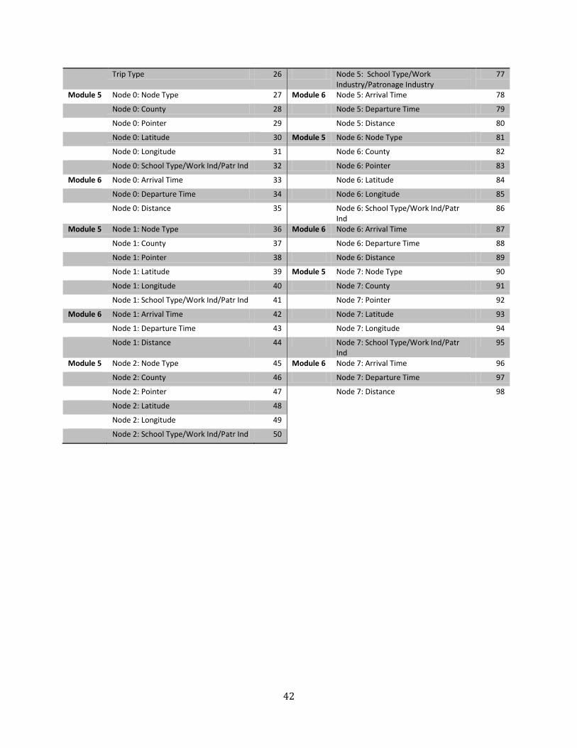
42

Trip Type 26 Node 5: School Type/Work Industry/Patronage Industry

77

Module 5 Node 0: Node Type 27 Module 6 Node 5: Arrival Time 78

Node 0: County 28 Node 5: Departure Time 79

Node 0: Pointer 29 Node 5: Distance 80

Node 0: Latitude 30 Module 5 Node 6: Node Type 81

Node 0: Longitude 31 Node 6: County 82

Node 0: School Type/Work Ind/Patr Ind 32 Node 6: Pointer 83

Module 6 Node 0: Arrival Time 33 Node 6: Latitude 84

Node 0: Departure Time 34 Node 6: Longitude 85

Node 0: Distance 35 Node 6: School Type/Work Ind/Patr Ind

86




Node 1: Latitude 39 Module 5 Node 7: Node Type 90

Node 1: Longitude 40 Node 7: County 91

Node 1: School Type/Work Ind/Patr Ind 41 Node 7: Pointer 92

Module 6 Node 1: Arrival Time 42 Node 7: Latitude 93

Node 1: Departure Time 43 Node 7: Longitude 94

Node 1: Distance 44 Node 7: School Type/Work Ind/Patr Ind

95




Node 2: Latitude 48

Node 2: Longitude 49

Node 2: School Type/Work Ind/Patr Ind 50

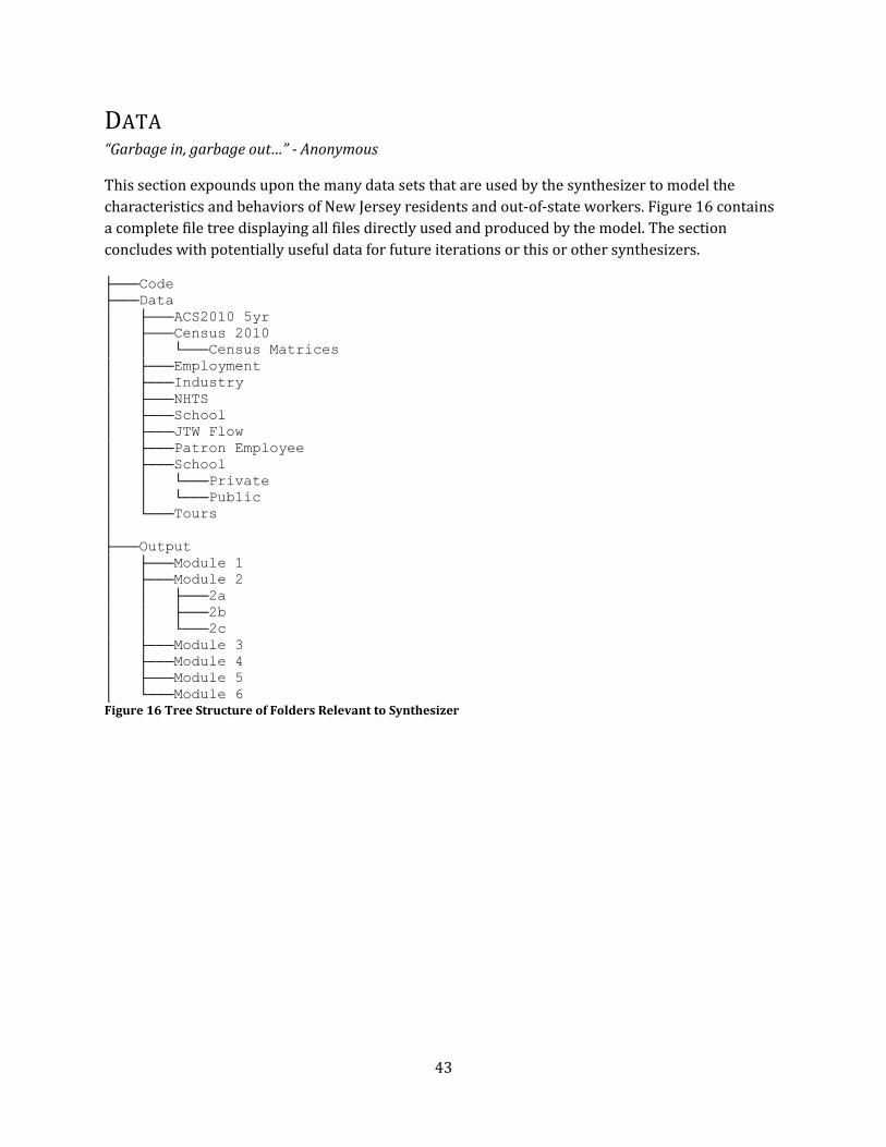
43

DATA “Garbage in, garbage out…” - Anonymous

This section expounds upon the many data sets that are used by the synthesizer to model the

characteristics and behaviors of New Jersey residents and out-of-state workers. Figure 16 contains

a complete file tree displaying all files directly used and produced by the model. The section

concludes with potentially useful data for future iterations or this or other synthesizers.

├───Code

├───Data

│ ├───ACS2010 5yr

│ ├───Census 2010

│ │ └───Census Matrices

│ ├───Employment

│ ├───Industry

│ ├───NHTS

│ ├───School

│ ├───JTW Flow

│ ├───Patron Employee

│ ├───School

│ │ └───Private

│ │ └───Public

│ └───Tours

│

├───Output

│ ├───Module 1


│ │ ├───2a

│ │ ├───2b

│ │ └───2c




│ └───Module 6

Figure 16 Tree Structure of Folders Relevant to Synthesizer

44

2010 CENSUS SUMMARY FILE 1 DATA It should first be noted that with the vast amount of Census Data that is publicly available, there are

actually several official places from which the data can be attained. In its raw form, however, the

data can be downloaded directly from ftp2.census.gov. A more complete link to the exact New

Jersey data can be found in the References section. However these data do require preprocessing,

first as detailed in the Readme file found in the ftp directory of the site (Summary File 1, 2011).

Following all instructions will give the user access to a 2.2 GB database file best opened using MS

Access 2007 or later. To save the user the trouble of then creating an appropriate table for the

needs of this project’s synthesizer, a VBA program is included (Appendix 1) to create 21 comma-

delimited text files named as such, “CountyCensusMatrix.txt” where County is one of the 21 County

in New Jersey using queries and then exporting the resulting tables to text files.

All entries in these files are numeric, allowing a fast reader like loadtxt from the Numpy package to

be used, and are at the block level only. To increase memory efficiency further, the fields INTPTLAT

(Latitude) and INTPTLON (Longitude) are read in a separate matrix as FLOAT data type. All other

fields are integers and read into an INT type matrix. A partial representation of all SF1 data used

here is found on the next page in Table 8. Note that some tables are pulled in their entirety such

that their field label starts at 1, such as HH_REL_DIST which starts at P0290001; while others start

higher as the previous fields are unnecessary; for example, GROUP_QUARTERS starts at field

P0430005. This is due to how the SQL queries used in the VBA script were built; that is with the

least amount of necessary data to be read. The field labels, as seen in the first row of Table 8,

correspond exactly to both the tables created by the queries as well as the original tables used by

the SF1 MS Access file. A complete reference to all fields can be found in chapter 5 of the 2010

Census of Population and Housing Technical Documentation (2012).

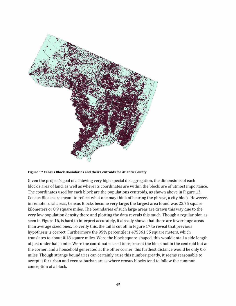
45

Figure 17 Census Block Boundaries and their Centroids for Atlantic County

Given the project’s goal of achieving very high special disaggregation, the dimensions of each

block’s area of land, as well as where its coordinates are within the block, are of utmost importance.

The coordinates used for each block are the populations centroids, as shown above in Figure 13.

Census Blocks are meant to reflect what one may think of hearing the phrase, a city block. However,

in remote rural areas, Census Blocks become very large: the largest area found was 22.75 square

kilometers or 8.9 square miles. The boundaries of such large areas are drawn this way due to the

very low population density there and plotting the data reveals this much. Though a regular plot, as

seen in Figure 16, is hard to interpret accurately, it already shows that there are fewer huge areas

than average sized ones. To verify this, the tail is cut off in Figure 17 to reveal that previous

hypothesis is correct. Furthermore the 95% percentile is 475361.55 square meters, which

translates to about 0.18 square miles. Were the block square-shaped, this would entail a side length

of just under half a mile. Were the coordinates used to represent the block not in the centroid but at

the corner, and a household generated at the other corner, this furthest distance would be only 0.6

miles. Though strange boundaries can certainly raise this number greatly, it seems reasonable to

accept it for urban and even suburban areas where census blocks tend to follow the common

conception of a block.

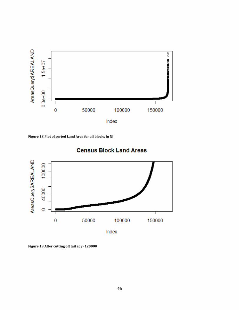
46

Figure 18 Plot of sorted Land Area for all blocks in NJ

Figure 19 After cutting off tail at y=120000

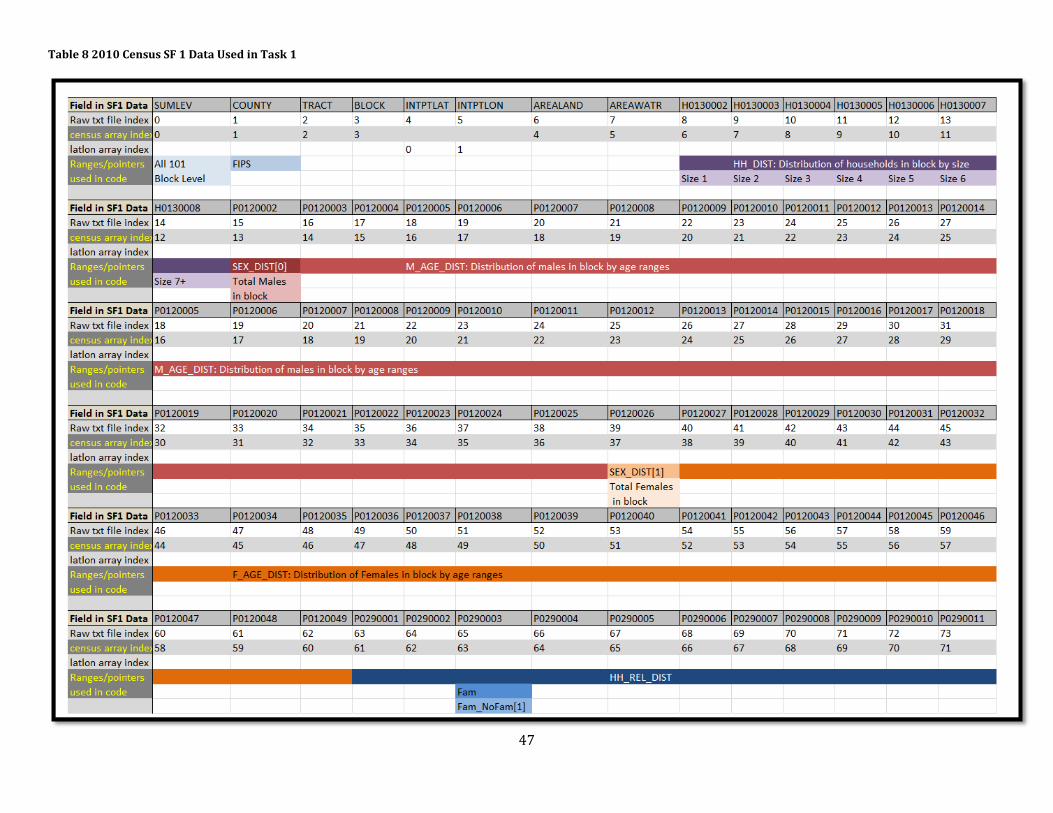
47

Table 8 2010 Census SF 1 Data Used in Task 1

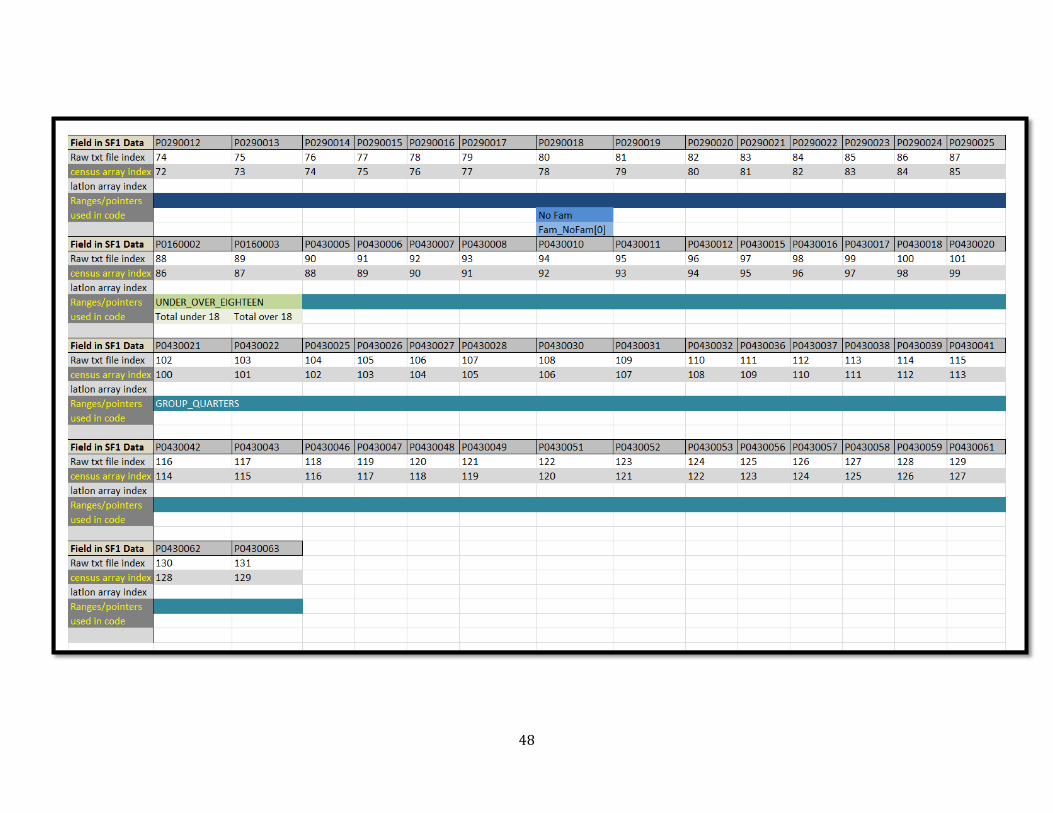
48

49

AMERICAN COMMUNITY SURVEY The ACS is an ongoing statistical survey that is also performed by the US Census Bureau. It samples

about 3 million people a year, trading some sampling error for the ability to ask more questions and

produce more detailed data from its surveys. It is meant to supplement the wide-coverage but short

form surveys of the decennial Census (American Communty Survey, 2012). A few data tables from

the American Community Survey are used by the synthesizer, specifically from the 2010 5-Year ACS

and 2010 3-Year ACS. These can very easily be retrieved by using the US Census FactFinder

(FactFinder, 2012) website and/or swapped out for other equivalent datasets (with file paths

changed appropriately). A full distinction between the 1-year, 3-year, and 5-year data sets can be

found on the ACS website (When to use 1-year, 3-year, or 5-year estimates, 2011). The longer

surveys have less sampling error (due to larger sample) and better specificity to analyzing small

populations (due to better scatter of samples); however, they are less current due to the sampling

being spread over 3 or 5 years.

The most important table from the ACS used here, is the ACS_10_5YR_S1910 which contains

distributions of household income by household type at the Census Tract level (the lowest public

available). These data are used in Task 1 to assign households and income bracket. A similar table

exists for individuals rather than households.

It is also worth noting that for every estimate in an ACS data table there is margin of error that is

given. These were not factored in for two main reasons. First, they were generally consistent and

small in magnitude, and second, the estimates were used as weights to draw from, that is as a

discrete distribution, and not to fit any sort of closed-form probability distribution around each

value or a set of values.

SCHOOL DATA SETS Another ACS data set used, ACS_10_3YR_S1401, contains data about private versus public school

enrollments by grade and age range at the County level, and includes the age groups 3-4, 5-9, 10-14,

15-17, 18-19, 20-24, and so on. Once again, only the estimates from this table, and not the margins

of error, were used in Task 3. Many other data sets had to be gathered from different sources to be

able to generate educational characteristics that are representative of actual students in New

Jersey. They are described here.

The October 2009 Current Population Survey contains several data tables regarding student

enrollment. The table "Enrollment Status of the Population 3 years old and over” provides the

number of students enrolled by education level and age at the national level. The categories for

education level are Nursery/Kindergarten, Elementary schools, High schools,

Undergraduate/Graduate, and Not Enrolled. Since Middle school is not actually specified, the line is

drawn such that students above ten years old are considered middle schoolers. A more detailed

distribution of middle schoolers versus elementary schoolers by age could not be ascertained and

so the aforementioned simplifying assumptions were made. The age ranges used are 3-4, 5-6, 7-9,

10-13, 14-15, 16-17, 18-19, 20-21, 22-24, 25-29, and so on. Enrollment numbers after the age of 29

are very low, and those in the 25-29 age bracket are reasonably low as well. As such, 22-24 is the

oldest bracket used to keep in line with the simplifying assumption of this model. It is a reasonable

50

one, since many residents over the age of 24 who are, for example graduate students, are also

counted as employees at their universities; therefore their trips should be accounted for by Module

2 when assigning workplaces.

Data on public schools are very easy to find. So much so that a few different organizations each have

their own datasets with different amounts of information for all the schools listed. The most

important data fields for the purposes of this synthesizer are the type of school or grade range,

enrollment numbers, and latitude and longitudinal coordinates (other potentially useful fields

include enrollment by grade and school district code). With these requirements in mind, the data

set for public schools was retrieved from the NJ Department of Education’s 2010 enrollment file,

and then separated into files for elementary, middle, high, and special schools.

A great deal of searching was needed to attain enrollment numbers for private schools. These data

were found and downloaded from the National Center of Education Statistics Website which

performs a yearly survey of private schools across the nation (Private School Universe Survey,

2009-2010).

Lastly university and college enrollments were also easily attainable from the New Jersey

government website (Fall 2011 Enrollment in New Jersey Colleges and Universities, 2011). This list

was divided into two files, Commuter and Non-commuter. The former list includes every

community college in the state as well as few more such the University of Phoenix and DeVry

University campuses and some other public institutions. The Non-commuter Universities/Colleges

file includes the remaining universities such as Rider, Princeton, Rutgers, NJIT and many more. One

glaring problem with this list, however, is that not all schools are listed separately by campus. In

addition to this, though the two categories created are meant to reflect the different living and thus

behavioral patterns of attendees of the institutions in those categories, some institutions were

placed in lists by assumption rather than by exploration of their student demographics. That is to

say, a more rigorous run through the colleges and universities in future endeavors can allow for

characteristics that more in line with those of college students in New Jersey.

EMPLOYERS AND PATRONAGE DATA The dataset containing businesses from which work places and places of patronage are picked was

obtained internally from a private source. It was intended to contain every business in the state of

New Jersey, however, at present it is unclear what percent of businesses may be missing and

whether there are any biases to certain industries caused by this. Nevertheless, the output when

using these data appears reasonable, as is demonstrated in the Results section. Every business in

the file contains many attributes including name, number of workers, NAICS code, county, street

address, latitude and longitude coordinates. NAICS codes are 8 digit indicators of industry type for

places of employment, where the first two digits from the left give a very general industry category

and every subsequent digit adds greater detail to the exact industry which the business falls under.

Due to the complexity of using so many digits, as well as the lack of data which can be matched at

such a high level, these code are truncated to the 3 left-most digits and appended after the Primary

NAICS column.

51

The availability of a latitude and longitude for every business (or at least a street address to be

geocoded) is what makes this dataset crucial. Even an incomplete dataset such as this one allows

for much more precise spatial distribution than Worker densities, Traffic Assignment Zones (TAZ),

or EPA zoning codes, which are commonly used in more traditional models. (Koppelman & Bhat,

2003)

There are many other fields in the original file that were discarded in the files read by Modules 2

and 4. A few noteworthy ones for future endeavors are whether the place is a home business and

whether it is a branch or a main office.

The same files used for businesses are used for patronage data with only a few simple

modifications. It was hypothesized that if for every NAICS code, a ratio of Average Daily Patronage

to Worker would make for a simple way to mimic daily patronage numbers while at the same time

retaining the same high level of spatial resolution that the synthesizer aims to do. As with before

however truncating the 8 digit NAICS codes was necessary if there was any hope of creating a table

of such ratios. Even with that, however, it appears that no such attempt has been made before and

so data for such a ratio doesn’t exist. Credit must be given to Bharath Alamanda of the ORF 467

class who during the previous incarnation of the synthesizer, performed the task of truncating

NAICS codes and creating Patron:Worker ratios to all two-digit codes. These ratios were reused this

time around as well, mainly due to time constraints as well as the lack of any clear data on which to

base the ratios on. In addition, if to be redone, it would be best if at least 3-digit NAICS codes were

used and an exact Patron:Worker ratio was actually drawn from a distribution, the parameters of

which were listed in the businesses file, instead of a constant ratio.

SCHEDULE FILES Module 6 reads in two files, for schools and businesses respectively, containing the fields:

minimum, maximum, and mode for both arrival and departure time for every school type and for

every 2-digit industry code, respectively. These parameters are used in triangular distributions that

will be used to draw a random time of arrival and/or departure. This distribution was chosen for its

simplicity in allowing a highly asymmetric distribution, which is useful in modeling, for example,

how more people should arrive early for school than late. The mode parameters generally reflect

the bell times of a school or start and end times for work.

While the bell times are essentially rounded averages for each school type for the entire state

rather than at the county-level, the variations in actual bell times are generally minor enough that

the data used still reflects the times at which students in New Jersey arrive at and leave schools. The

same cannot be said for different industries. First, as previously mentioned, the industries are

rather aggregated within their 2-digit industry codes, which causes the times set to less accurately

represent all different types of businesses within the code. Additionally, the data for every industry

is unimodal, that is to say, occurs during a single shift. For those who work after school, the arrival

and departure parameters are simply incremented such that they cannot overlap with school

timings. See the Conclusions, Limitations, and Next Steps section for both a simple way to

implement dual shifts without adding any data, as well as how to replace Tasks 4, 5, and 6 with a

much more comprehensive activity-based location selection model.

52

DATA FOR FUTURE PROJECTS Early in the project, several ideas not included in the current synthesizer were considered to

capture with even greater accuracy the characteristics of New Jersey residents. Some of these ideas

will be explained further in the Limitations and Next Steps section under Worthwhile Increases in

Complexity. Some of the data sets with potential to be used in improving the synthesizer are listed

here.

Currently a single unemployment rate is used for the whole state (9.8% rounded up to 10%). This

can definitely be disaggregated to the county level using data from either the Quarterly Workforce

Indicator (LED, 2012) or from the Bureau of Labor Statistics (BLS, 2012).

In this version of the synthesizer, household locations are simply the centroid coordinates of the

Census Block they are in. There are several ways in which these households can be distributed

reasonably within the block. At least a few of these ways could benefit from EPA zoning data and/or

Traffic Assignment Zone data that can inform the synthesizer of the type of buildings/residences in

a particular block. This could also be achieved on some level by merely creating block level density

of population over land area of the block. With data such as these, Real Estate/Housing Value data

from Zillow.com could then be used to match households that are likely to afford such real estate,

and from this find where to place that household. This is briefly elaborated on in the Limitations

and Next Steps Section.

Lastly, the American Time Use Survey (BLS, 2012) and the 2009 National Household Travel Survey

(NHTS, 2011) contains data that can be useful in better modeling Mobility Behavior, as well as the

durations spent recreating depending on the type.

53

RESULTS “The guts of it.”

With output from several runs of all 6 modules produced, it is now prudent to assess how accurate

the results are. The first order estimation of this is done simply by comparing with the

distributions of input data with output data. The frequent random sampling performed in this

synthesizer, albeit approximate and based on pseudorandom number generators, should result in

distributions matching those that were used as input, and thus, create characteristics that are

representative of the New Jersey population and their behavior. Next, aggregate values from the

output, such as county worker populations, are compared to their real values. These act as

benchmarks that indicate that nothing is lost through the use more disaggregated inputs. Lastly,

distributions of different attributes generated by the synthesizer are compared graphically and

heuristically. These include age, income, and trip distance distributions. Note that the exact

numbers tabulated below were chosen out of several possible output sets to be representative of

the output of the Synthesizer. Some tables were created based on output files from different runs

and such numbers across tables may not all correspond perfectly.

ATTRIBUTES OF THE SYNTHETIC POPULATION AND ITS WORKERS First it is confirmed that the total populations of each county are almost exactly as listed in the

2010 Census, as seen in Table 9, thanks to deterministically using the exact population of every

Census Block to generate residents. It isn’t certain how the module can result in a higher population

output than the data; however, the outputs that are slightly lower than the real numbers can be

explained by the fact that households created have at most 7 people in them, while in the Census

data, the relevant data field is in fact for 7 or more people.

Table 9 County Populations: Output and Census Numbers

County Output Census 2010 Population % Difference

Atlantic 272,552 274,549 -0.7274 Bergen 907,113 905,116 0.2206 Burlington 448,523 448,734 -0.0470 Camden 513,868 513,657 0.0411 Cape May 97,259 97,265 -0.0062 Cumberland 156,904 156,898 0.0038 Essex 783,969 783,969 0.0000 Gloucester 288,288 288,288 0.0000 Hudson 634,266 634,266 0.0000 Hunterdon 128,349 128,349 0.0000 Mercer 365,012 366,513 -0.4095 Middlesex 811,359 809,858 0.1853 Monmouth 630,380 630,380 0.0000 Morris 492,276 492,276 0.0000 Ocean 576,562 576,567 -0.0009 Passaic 501,225 501,226 -0.0002 Salem 66,088 66,083 0.0076 Somerset 323,445 323,444 0.0003 Sussex 149,265 149,265 0.0000 Union 536,499 536,499 0.0000

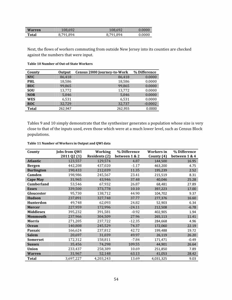
54

Warren 108,692 108,692 0.0000

Total 8,791,894 8,791,894 0.0000

Next, the flows of workers commuting from outside New Jersey into its counties are checked

against the numbers that were input.

Table 10 Number of Out-of-State Workers

County Output Census 2000 Journey-to-Work % Difference

NYC 86,418 86,418 0.0000 PHL 18,586 18,586 0.0000 BUC 99,865 99,865 0.0000 SOU 13,772 13,772 0.0000 NOR 5,046 5,046 0.0000 WES 6,531 6,531 0.0000 ROC 32,729 32,737 -0.0002

Total 262,947 262,955 0.0000

Tables 9 and 10 simply demonstrate that the synthesizer generates a population whose size is very

close to that of the inputs used, even those which were at a much lower level, such as Census Block

populations.

Table 11 Number of Workers in Output and QWI data

County Jobs from QWI 2011 Q2 (1)

Working Residents (2)

% Difference between 1 & 2

Workers in County (4)

% Difference between 1 & 4

Atlantic 123,557 129,574 4.87 144,500 16.95 Bergen 442,208 437,020 -1.17 463,200 4.75 Burlington 190,433 212,039 11.35 195,239 2.52 Camden 198,986 245,567 23.41 215,519 8.31 Cape May 31,965 43,946 37.48 40,046 25.28 Cumberland 53,546 67,932 26.87 68,481 27.89 Essex 339,500 373,778 10.10 397,223 17.00 Gloucester 95,730 138,712 44.90 104,702 9.37 Hudson 237,891 327,748 37.77 277,376 16.60 Hunterdon 49,748 62,093 24.82 52,903 6.34 Mercer 227,959 172,996 -24.11 212,508 -6.78 Middlesex 395,232 391,581 -0.92 402,905 1.94 Monmouth 237,966 304,509 27.96 265,113 11.41 Morris 271,205 237,722 -12.35 284,668 4.96 Ocean 140,808 245,529 74.37 172,060 22.19 Passaic 166,624 237,812 42.72 199,488 19.72 Salem 20,697 31,039 49.97 26,119 26.20 Somerset 172,312 158,811 -7.84 171,471 -0.49 Sussex 35,456 74,298 109.55 44,901 26.64 Union 233,437 258,389 10.69 251,850 7.89 Warren 31,967 52,148 63.13 41,053 28.42

Total 3,697,227 4,203,243 13.69 4,031,325 9.03

55

Next, worker numbers for every county are compared to numbers from the 2011 Q2 figures of the

Quarterly Workforce Indicators (LED, 2012). Table 11 below looks at the number of all workers in

each county.

First it should be noted that the QWI numbers in column 1 of Table 11 are not actually of workers

but of jobs, so these figures could potentially be higher than those of the actual number of workers

since some workers could potentially hold more than one job. Still, this is not the case in the

Synthesizer’s population model and the numbers in columns 2 and 4 are mostly greater than those

in column 1. The total number of full-time workers generated is about 14% higher than the QWI

figures. That said, however, the total number of workers according to the 2010 3-yr ACS is

4,237,908; which is much closer to the number of Traveler Type 5s from the Synthesizer output.

Based on the larger percent differences on a county level than on the state level, it is very likely that

the use of a single unemployment rate for the entire state has caused several counties to have far

too many workers, while others too few. Furthermore, the numbers seen in the first data column of

Table 11 are workers who live in their respective counties, but not necessarily work in them. On the

other hand those in column 4 work in the counties listed but do not necessarily live in them.

Counties with a large difference between columns 2 and 4 are evidently ones with a high degree of

out-of-county commuting. For such counties, like Sussex and Warren, the column 1 figures poorly

reflect the numbers of workers who commute to work daily. Similarly the totals of columns 2 and 4

are likely different because column 4 does not include those who leave the state for work.

Furthermore, the synthesizer produced far too few residents who both work and go to high school.

The synthesizer output contains just over 5,000 such school-age workers (TT 2), about 15 times

fewer than the 75 thousand jobs held by residents ages 14 to 18, according to the QWI 2011 Q2

(LED, 2012), but exactly 0.194 percent of the total number of school-age residents (TT’s 1 and 2) as

was input. This percentage was calculated erroneously from the QWI numbers and was thought to

be a percent of the total number of school-aged children, but in fact is a percent of school-aged

working children (under 19) to all workers. The latest version of Module 1 uses an updated

percentage and this will be reflected in all later runs

Next, Figure 20 Populations by County and Sex from Synthesizer Outputand Figure 21 are

juxtaposed to show that the female to male ratios of the output are perfectly preserved by the

synthesizer. The state-wide cumulative distributions of ages in Figure 22 and Figure 23 also match

well. The numbers of bins in these two charts differ because of the fact that the Census data is given

in age ranges while the synthesizer output gives exact ages. Furthermore, the number of people

above the age of 85 seems less than expected; however, this has no bearing on the model used by

this synthesizer as they are considered non-travelers.

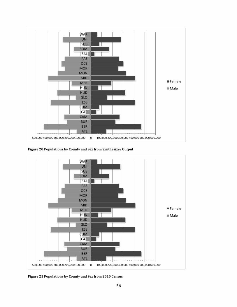
56

Figure 20 Populations by County and Sex from Synthesizer Output

Figure 21 Populations by County and Sex from 2010 Census

500,000 400,000 300,000 200,000 100,000 0 100,000 200,000 300,000 400,000 500,000 600,000

ATL

BER

BUR

CAM

CAP

CUM

ESS

GLO

HUD

HUN

MER

MID

MON

MOR

OCE

PAS

SAL

SOM

SUS

UNI

WAR

Female

Male

500,000 400,000 300,000 200,000 100,000 0 100,000 200,000 300,000 400,000 500,000 600,000

ATL

BER

BUR

CAM

CAP

CUM

ESS

GLO

HUD

HUN

MER

MID

MON

MOR

OCE

PAS

SAL

SOM

SUS

UNI

WAR

Female

Male

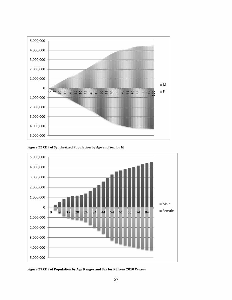
57

Figure 22 CDF of Synthesized Population by Age and Sex for NJ

Figure 23 CDF of Population by Age Ranges and Sex for NJ from 2010 Census

5,000,000

4,000,000

3,000,000

2,000,000

1,000,000

0

1,000,000

2,000,000

3,000,000

4,000,000

5,000,000

0 5

10

15

20

25

30

35

40

45

50

55

60

65

70

75

80

85

90

95

10

0

M

F

5,000,000

4,000,000

3,000,000

2,000,000

1,000,000

0

1,000,000

2,000,000

3,000,000

4,000,000

5,000,000

0 9 17 20 24 34 44 54 61 66 74 84

Male

Female

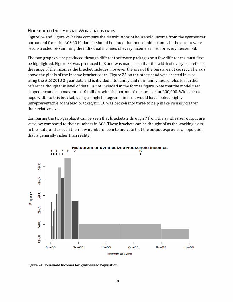
58

HOUSEHOLD INCOME AND WORK INDUSTRIES Figure 24 and Figure 25 below compare the distributions of household income from the synthesizer

output and from the ACS 2010 data. It should be noted that household incomes in the output were

reconstructed by summing the individual incomes of every income earner for every household.

The two graphs were produced through different software packages so a few differences must first

be highlighted. Figure 24 was produced in R and was made such that the width of every bar reflects

the range of the incomes the bracket includes, however the area of the bars are not correct. The axis

above the plot is of the income bracket codes. Figure 25 on the other hand was charted in excel

using the ACS 2010 3-year data and is divided into family and non-family households for further

reference though this level of detail is not included in the former figure. Note that the model used

capped income at a maximum 10 million, with the bottom of this bracket at 200,000. With such a

huge width to this bracket, using a single histogram bin for it would have looked highly

unrepresentative so instead bracket/bin 10 was broken into three to help make visually clearer

their relative sizes.

Comparing the two graphs, it can be seen that brackets 2 through 7 from the synthesizer output are

very low compared to their numbers in ACS. These brackets can be thought of as the working class

in the state, and as such their low numbers seem to indicate that the output expresses a population

that is generally richer than reality.

Figure 24 Household Incomes for Synthesized Population

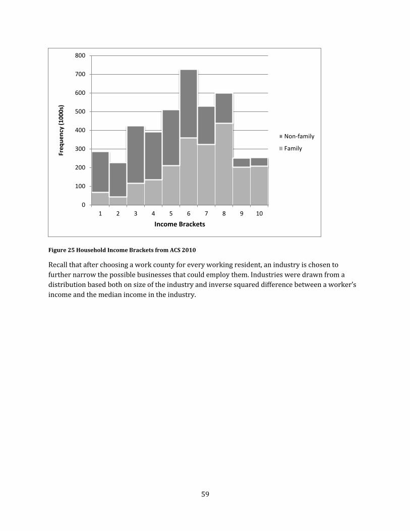
59

Figure 25 Household Income Brackets from ACS 2010

Recall that after choosing a work county for every working resident, an industry is chosen to

further narrow the possible businesses that could employ them. Industries were drawn from a

distribution based both on size of the industry and inverse squared difference between a worker’s

income and the median income in the industry.

0

100

200

300

400

500

600

700

800

1 2 3 4 5 6 7 8 9 10

Fre

qu

en

cy (

10

00

s)

Income Brackets

Non-family

Family

60

STUDENT POPULATIONS NUMBERS Next the numbers of students and their distribution by student type is explored. Though now fixed,

the code used at the time of writing contained a bug that resulted in output that did not assign any

private schools to students. According to the 2010 ACS data, this represents about 12% student

enrollment. As such the spatial distribution of schools destinations in the output is less

representative of reality than future iterations of the synthesizer. The total numbers of students in

different grade levels are compared in Table 13 below.

Table 12 Student Type distributions of Synthesized Population and ACS 2010

Students in Synthesized Population Students According to ACS 2010 Student Type # Population Total Total Population Student Type Public Elementary 0 535,217 916,495 1,030,002 117,180 Kindergarten Public Middle 1 381,278 450,923 Grades 1-4 461,899 Grades 5-8 Public High 2 472,476 472,476 502,073 502,073 Grades 9-12 Commuter Uni/College 7 242,884 319,061 576,938 456,431 Undergraduate Non-commuter Uni/College

8 76,177 120,507 Graduate/Prof.

Special Needs 6 13,983 13,983

As mentioned back in the section on assigning schools, most data sets found did not contain data

specific to middle school, but either included it in the data on elementary schools or created a

division different than elementary/middle. Since the middle school distinction was created using

age in the synthesizer, the number of middle school students will be added to elementary school

students. The commuter/non-commuter distinction in university and colleges was also one made

only for the purposes of the synthesizer so these values are summed together and compared to the

sum of undergraduate and graduate students in Table 13.

The number of students in the synthesized population is somewhat low across all grade levels, most

notably the number of college students. This is likely due to the fact that the cutoff age for students

was set to 22, which excludes a large number of potential students, making them workers or

homeworkers instead. This also supports the reasoning behind the high number of workers from

before.

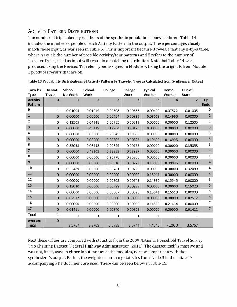
61

ACTIVITY PATTERN DISTRIBUTIONS The number of trips taken by residents of the synthetic population is now explored. Table 14

includes the number of people of each Activity Pattern in the output. These percentages closely

match those input, as was seen in Table 5. This is important because it reveals that any n-by-8 table,

where n equals the number of possible activity/tour patterns and 8 refers to the number of

Traveler Types, used as input will result in a matching distribution. Note that Table 14 was

produced using the Revised Traveler Types assigned in Module 4. Using the originals from Module

1 produces results that are off.

Table 13 Probability Distributions of Activity Pattern by Traveler Type as Calculated from Synthesizer Output

Traveler Type

Do-Not-Travel

School-No-Work

School-Work

College College-Work

Typical Worker

Home-Worker

Out-of-State

Activity Pattern

0 1 2 3 3 5 6 7 Trip Ends

0 1 0.01005 0.01019 0.00508 0.00658 0.00400 0.07522 0.01005 0

1 0 0.00000 0.00000 0.00794 0.00859 0.05013 0.14990 0.00000 2

2 0 0.12505 0.04948 0.00785 0.00819 0.00000 0.00000 0.12505 2

3 0 0.00000 0.40439 0.19964 0.20170 0.00000 0.00000 0.00000 3

4 0 0.00000 0.00000 0.20045 0.19638 0.00000 0.00000 0.00000 3

5 0 0.00000 0.00000 0.00805 0.00823 0.19630 0.14995 0.00000 3

6 0 0.35058 0.08493 0.00829 0.00752 0.00000 0.00000 0.35058 3

7 0 0.00000 0.45102 0.25925 0.25857 0.00000 0.00000 0.00000 4

8 0 0.00000 0.00000 0.25778 0.25906 0.00000 0.00000 0.00000 4

9 0 0.00000 0.00000 0.00810 0.00779 0.15035 0.09996 0.00000 4

10 0 0.32489 0.00000 0.00781 0.00720 0.00000 0.00000 0.32489 4

11 0 0.00000 0.00000 0.00000 0.00000 0.15011 0.00000 0.00000 4

12 0 0.00000 0.00000 0.00802 0.00743 0.14980 0.15545 0.00000 5

13 0 0.15020 0.00000 0.00798 0.00855 0.00000 0.00000 0.15020 5

14 0 0.00000 0.00000 0.00507 0.00528 0.15041 0.15518 0.00000 5

15 0 0.02512 0.00000 0.00000 0.00000 0.00000 0.00000 0.02512 5

16 0 0.00000 0.00000 0.00000 0.00000 0.14889 0.21434 0.00000 7

17 0 0.01411 0.00000 0.00870 0.00895 0.00000 0.00000 0.01411 7

Total 1 1 1 1 1 1 1 1

Average Trips

0 3.5767 3.3709 3.5788 3.5744 4.4346 4.2030 3.5767

Next these values are compared with statistics from the 2009 National Household Travel Survey

Trip Chaining Dataset (Federal Highway Administration, 2011). The dataset itself is massive and

was not, itself, used in either input for any of the modules, nor for comparison with the

synthesizer’s output. Rather, the weighted summary statistics from Table 3 in the dataset’s

accompanying PDF document are used. These can be seen below in Table 15.

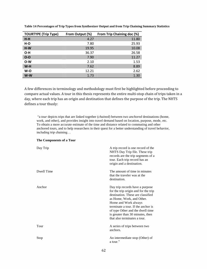
62

Table 14 Percentages of Trip Types from Synthesizer Output and from Trip Chaining Summary Statistics

TOURTYPE (Trip Type) From Output (%) From Trip Chaining doc (%)

H-H 4.27 11.80 H-O 7.80 25.93 H-W 19.95 10.08 O-H 36.37 26.58 O-O 7.90 11.27 O-W 2.10 1.53 W-H 7.62 8.89 W-O 12.21 2.62 W-W 1.73 1.30

A few differences in terminology and methodology must first be highlighted before proceeding to

compare actual values. A tour in this thesis represents the entire multi-stop chain of trips taken in a

day, where each trip has an origin and destination that defines the purpose of the trip. The NHTS

defines a tour thusly:

“a tour depicts trips that are linked together (chained) between two anchored destinations (home,

work, and other), and provides insight into travel demand based on location, purpose, mode, etc.

To obtain a more accurate estimate of the time and distance related to commuting and other

anchored tours, and to help researchers in their quest for a better understanding of travel behavior,

including trip chaining…

The Components of a Tour

Day Trip

A trip record is one record of the

NHTS Day Trip file. These trip

records are the trip segments of a

tour. Each trip record has an

origin and a destination.

Dwell Time The amount of time in minutes

that the traveler was at the

destination.

Anchor Day trip records have a purpose

for the trip origin and for the trip

destination. These are classified

as Home, Work, and Other.

Home and Work always

terminate a tour. If the anchor is

of type Other and the dwell time

is greater than 30 minutes, then

that also terminates a tour.

Tour A series of trips between two

anchors.

Stop An intermediate stop (Other) of

a tour.”

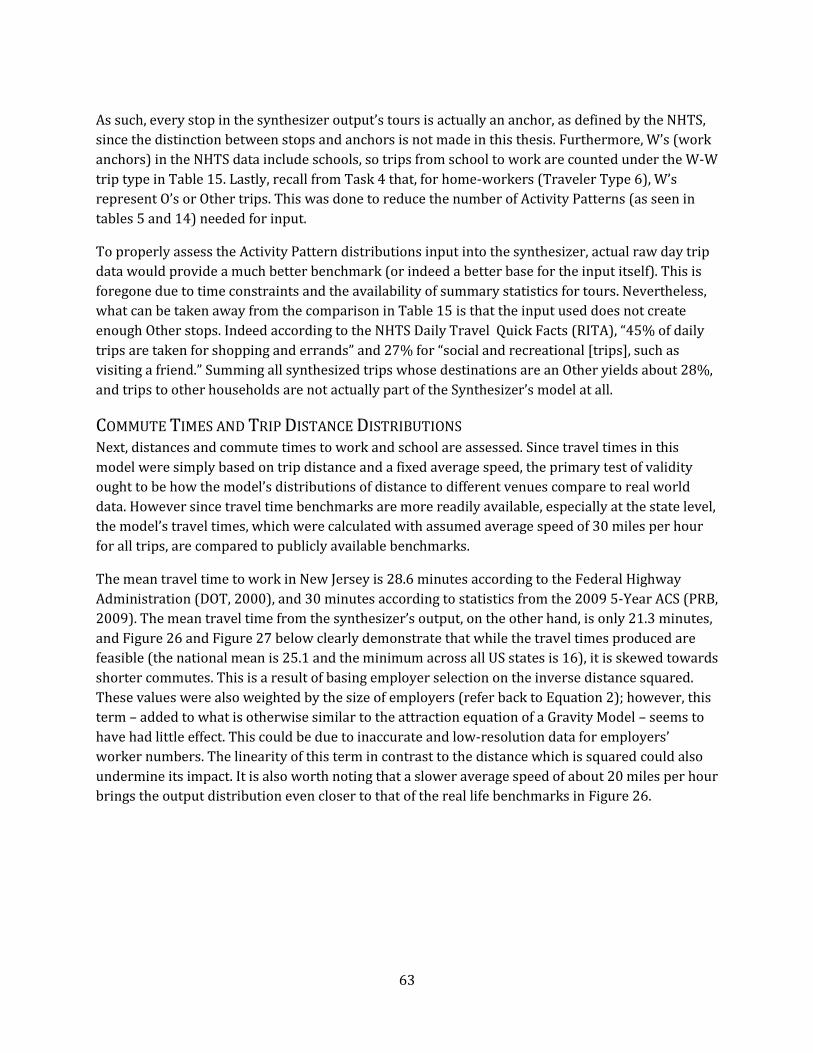
63

As such, every stop in the synthesizer output’s tours is actually an anchor, as defined by the NHTS,

since the distinction between stops and anchors is not made in this thesis. Furthermore, W’s (work

anchors) in the NHTS data include schools, so trips from school to work are counted under the W-W

trip type in Table 15. Lastly, recall from Task 4 that, for home-workers (Traveler Type 6), W’s

represent O’s or Other trips. This was done to reduce the number of Activity Patterns (as seen in

tables 5 and 14) needed for input.

To properly assess the Activity Pattern distributions input into the synthesizer, actual raw day trip

data would provide a much better benchmark (or indeed a better base for the input itself). This is

foregone due to time constraints and the availability of summary statistics for tours. Nevertheless,

what can be taken away from the comparison in Table 15 is that the input used does not create

enough Other stops. Indeed according to the NHTS Daily Travel Quick Facts (RITA), “45% of daily

trips are taken for shopping and errands” and 27% for “social and recreational [trips], such as

visiting a friend.” Summing all synthesized trips whose destinations are an Other yields about 28%,

and trips to other households are not actually part of the Synthesizer’s model at all.

COMMUTE TIMES AND TRIP DISTANCE DISTRIBUTIONS Next, distances and commute times to work and school are assessed. Since travel times in this

model were simply based on trip distance and a fixed average speed, the primary test of validity

ought to be how the model’s distributions of distance to different venues compare to real world

data. However since travel time benchmarks are more readily available, especially at the state level,

the model’s travel times, which were calculated with assumed average speed of 30 miles per hour

for all trips, are compared to publicly available benchmarks.

The mean travel time to work in New Jersey is 28.6 minutes according to the Federal Highway

Administration (DOT, 2000), and 30 minutes according to statistics from the 2009 5-Year ACS (PRB,

2009). The mean travel time from the synthesizer’s output, on the other hand, is only 21.3 minutes,

and Figure 26 and Figure 27 below clearly demonstrate that while the travel times produced are

feasible (the national mean is 25.1 and the minimum across all US states is 16), it is skewed towards

shorter commutes. This is a result of basing employer selection on the inverse distance squared.

These values were also weighted by the size of employers (refer back to Equation 2); however, this

term – added to what is otherwise similar to the attraction equation of a Gravity Model – seems to

have had little effect. This could be due to inaccurate and low-resolution data for employers’

worker numbers. The linearity of this term in contrast to the distance which is squared could also

undermine its impact. It is also worth noting that a slower average speed of about 20 miles per hour

brings the output distribution even closer to that of the real life benchmarks in Figure 26.

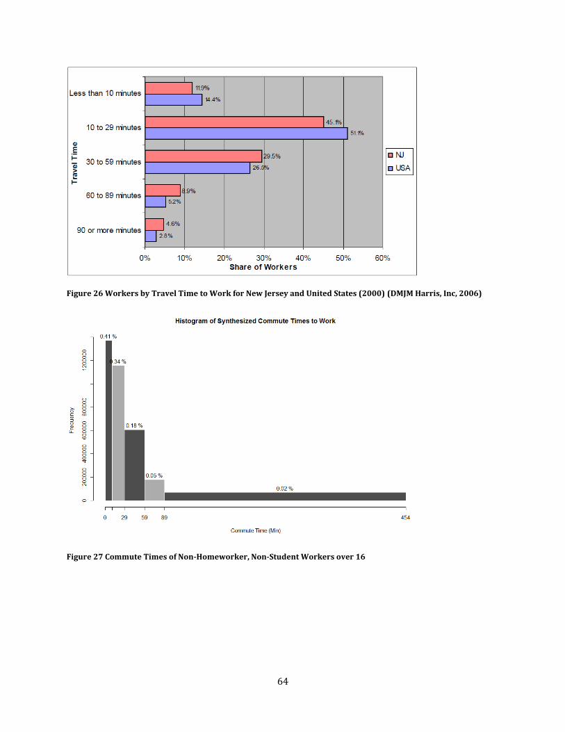
64

Figure 26 Workers by Travel Time to Work for New Jersey and United States (2000) (DMJM Harris, Inc, 2006)

Figure 27 Commute Times of Non-Homeworker, Non-Student Workers over 16

65

Though actual statistics or data with which to benchmark the output’s school distributions are hard

to find, conventional knowledge of schools can quickly reveal that the distances to school suffer of

the same problems distances to work did, only to a greater extent. The percentiles in Table 16 are

telling. Almost 90% of students go to schools that are only 4 miles away and 50% live less than a

mile away from school. Had this been reality there would not even be a need to create any separate

transportation for this purpose.

Table 15 Percentiles of Distances of Synthesized School Trips

Percentile 0% 10% 20% 30% 40% 50% 60% 70% 80% 90% 100%

Distance(mi) 0.01 0.23 0.37 0.51 0.68 0.89 1.17 1.58 2.29 4.17 145.21

Recall from Task 3 that all public K-12 schools were assigned by greatest proximity to home, and

that private schools (which are far fewer than public ones) and all colleges and universities were

selected using the modified attraction equation used repeatedly in this model; here based on

enrollment over squared distance. The limitations of this equation are discussed in the following

section.

Lastly, trip distances across all purposes are analyzed and compared. A look at the percentiles in

Table 17 reveals some heavy outliers and a more detailed look reveals that even the 98th percentile

is 52 miles, a still reasonable distance for a very long single trip.

Table 16 Percentiles of Distances of all Synthesized Trips

Percentile 10% 20% 30% 40% 50% 60% 70% 80% 90% 98% 100%

Distance(mi) 1.25 3.04 5.16 7.28 9.49 12.09 15.41 20.27 29.16 52.02 5,451.27

The mean of the unfiltered output (32.6 million trips) is just under 78 miles, however after

removing outliers by curtailing the distances at 170 miles, the mean is found to be 12.4 miles – just

3 miles over the national mean according to the 2009 Nationwide Personal Transportation Survey

(Energy Efficiency and Renewable Energy, 2012). A histogram of the output less than 70 miles can

be found on the next page in Figure 28, followed by the same output filtered to be below 10 miles.

Overall the distribution in Figure 28 fit the expected output of a Gravity Model, inverse

proportionality to squared distance, quite well. The only exception is the very first bin, or distances

under 2 miles of which there are more than hoped for. In Figure 29, it is clear that trips under half a

mile are significantly less than those closer to 1. This is likely due to the restriction of Other trips to

being of at least a half mile distance in Module 5. Still it did not do enough to reproduce a more

realistic distribution of distances where the bin frequencies should rise before going back down

and before resembling a quadratic curve. Such a monotonic curve arises due to the phenomenon in

which the places one needs to go are less likely to all be very close, reducing the number of possible

short trips despite one’s affinity to a shorter trip.

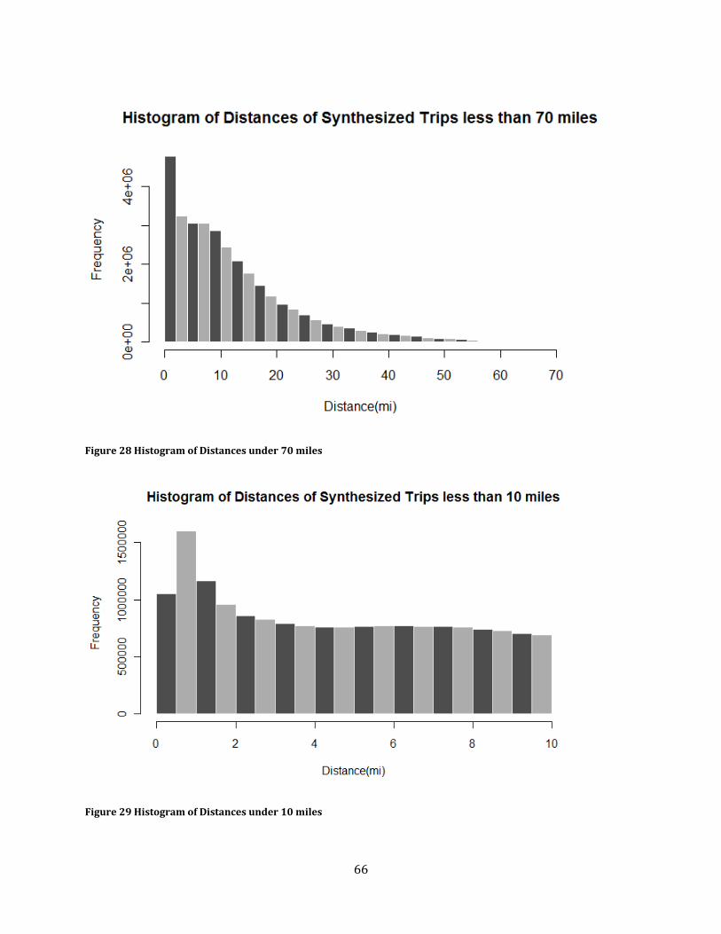
66

Figure 28 Histogram of Distances under 70 miles

Figure 29 Histogram of Distances under 10 miles

67

CONCLUSIONS, LIMITATIONS, AND NEXT STEPS In this section, conclusions about the results of the Synthesizer’s output are drawn, limitations–

intended or otherwise–are noted, and potential improvements are stated. Specifically, for each task

the goodness of the used methods and data are addressed for their strengths and weaknesses, as

well next steps to take in pursuing the goals of this thesis.

TASK 1 The output of Module 1 indicates that the methods used there are reasonable and valid for the

purpose of creating a populous with the characteristics of New Jersey, except for a few flaws.

Besides these flaws, addressed below, the methods used can likely be reproduced quite easily for

any other state in the country.

Though the data used as input in Module 1 has already been discussed both in the Methodology and

Data sections, it’s worth once again stating how vast the data that can be acquired from the

decennial Census and the American Community Survey. One limitation worth noting is that, for

privacy concerns, low populated areas have more aggregated data than otherwise, so when looking

only at block-level data, a small percentage of residents are glossed over. Statistically this is nearly

insignificant for the purposes of this model.

There are many tables and fields of data that could be of use in adding complexity to how the

synthetic population is created, but even more so that would likely be overkill. The Census includes

a table with the exact number of children of every age under 20 at the block level (P14 – Sex by Age

for the Population Under 20 Years Old); this would invariably add even greater, though

unnecessary, accuracy to the generation of school-aged residents. The Census also contains tables

containing the exact number of households containing people over 60, 65, and 75 – such data on the

other hand seem superfluous. There is greater data on family types, householder relationships, and

even car-ownership; all of which could be of potential use in synthesizing residents whose

characteristics match those of real residents in their location.

In addition, incomes assigned to households (and subsequently to workers) can without a doubt be

improved. One glaring issue is that while the model does read in household income distributions

across different income brackets and household types (family/non-family) at the Census Tract

level, it does not take into account the size of household or the number of workers. Only after

assigning a household income, are shares of the total income allocated to individual workers.

Integrating the use of individual income distributions (also available through ACS data) would

likely improve these results. One possible method would be to create distributions of individual

income, conditioned on household income.

Another income related suggestion involves acquiring data on land values and/or rent at the

Census Tract level and further integrating it into assigning household incomes.

Perhaps most importantly in a future iteration of such a synthesizer, after correcting any simple

numerical or coding errors mentioned in the results section, it would be imperative to use

unemployment numbers at the county level or lower, rather than at the state level as was used

68

here. Furthermore, categorizing employment into full-time and part-time would allow for better

Activity Pattern distributions in Task 4, as well as better numbers for working students.

Lastly, adding names to every resident in the synthetic population was desired but left out due to

time constraints. There are many ways this could be approached; however, most will ultimately be

limited due to whatever data sets can be found, especially if a probability distribution is desired

rather than a list where all names carry the same likelihood. A more promising solution was to

reverse look-up large areas in the White-Pages, from which a list of names can be produced, tallied,

and sampled. This however, cannot be done simply with the official White-Pages API as it only

allows for single person/address queries at any one time, as well as limiting these to 100 queries a

day. Other means to acquire a complete text format White-Pages Listing would have to be pursued.

TASK 2 Module 2’s overall goal is to correctly reflect the characteristics of workers in New Jersey, both

those from within (Module 2b) and from outside the state (Modules 2a and 2c). The methods used

to select industries and places of employment relied on attraction equations (generally a weight

over a squared distance) to create the distributions from which to draw.

For industries, distance was the difference between a worker’s income and the median income of a

certain industry, and the weighting factor was the size of the industry. Though the results were too

many and cumbersome to display in the Results section, analysis of the number of workers for

every industry as well their median incomes showed that the output did accurately recreate those

of the input. Further study is required to find a more suitable model for work industry selection.

One promising method would be to use a separate distribution of income for every industry by

county, rather than simply a median income. If such data were found, a conditional probability

distribution for every industry given the worker’s income could be created using Bayes’ theorem.

Better industry and income assignment would likely improve the overall distribution of where

people work. Currently incomes are first assigned to households and then divided evenly over all

working members. This can be improved in a number of ways, including using individual income

distribution, or dividing household income more intelligently based on householder relations,

household size, and/or sex.

For places of employment, distance was L-2 distance based on latitude/longitude coordinates and

the weighting factor was the number of workers at the branch or business. This model, which

mimics a traditional gravity model used in classic four step Transportation Models, produced

results that reasonably represented the expected worker behavior –aversion to working far away.

That said one of the biggest improvements would come from a better employer data. Not only a

more complete list of employers but more accurate employment numbers, or perhaps better square

footage data, which combined with industry type, could heuristically be used to gauge the number

of employees. Furthermore, including mobile employment in the model would better account for

jobs that involve traveling and would bring up the low average number of trips in the output.

Finally, another glaring aspect of employment that is in part missing from the current data sets is

employment numbers for schools, airports, and railway stations.

69

A method to ensure that the number of workers in each county was correct and in line with the

numbers in the Journey-to-Work census was also devised early on, but left out due to time

constraints and explained here briefly. First compare the number of workers generated (GWi) in

county i to sum of all workers who commute to work in county i (JTWi) from the Journey-to-Work

data; since this is commuter data, it should not include homeworkers. If GWi is greater than JTWi ,

define the probability of staying home, P(Staying Home) as in Equation 5 below, then iterate over

every worker and draw based on this probability whether or not the worker works at home or

commutes.

( ) ( )

Equation 5 Probability of staying home to adjust number of workers

If GWi is less than JTWi , determine how many workers the model is short, then iterate over all

eligible non-workers and draw from based on the absolute value of Equation 5 whether to convert a

non-worker to a worker. Finally check to see if new GWi = JTWi . Repeat if necessary.

TASK 3 The methods used to assign student types were ultimately found to be somewhat convoluted,

especially after first having to assign a Traveler Type in Task 1, a Student Type in Task 3, and then

in Task 4 a Revised Traveler Type, which simply sets school-aged children (TT’s 1 and 2) who were

not enrolled (ST 9) to Homeworkers (TT 6). In the future it would be best to use the enrollment

percent numbers early on in Task 1 to decide whether a school-aged child goes to school or not.

Then TT 2s (children over 15 who go to school and work) could also just be converted to TT 5.

Keeping a distinct Student Type indicator is reasonable as it allows for greater specificity in the

mobility patterns of students, i.e. by conditioning students’ Activity Patterns on Student Type rather

than just Traveler Type.

As discussed in the Data section, most of the ample datasets pertaining to schools and students are

not well standardized, using different age ranges, and different grade categories; many do not use

the term middle school at all. As such eliminating the middle school category would likely be best in

the future.

The distinction between college students that might commute to work as opposed to live on

campus was also not well established. Though it may be sound to say, for example, that the travel

behavior of Princeton students are very different than those of Bergen Community College, using

the same binary categorization to create a distinction between college students who work part time

and those who do not now seems erroneous. This distinction was actually ignored in the end due to

the realization that for some non-commuter colleges, students are just as likely to hold a part-time

job as those in a commuter college. This was further obfuscated by the choice of placing

Universities like Rutgers (which has only one listing despite having multiple campuses) in the Non-

Commuter list. Future iterations can improve on this in one of two possible ways. The conservative

way is to simply make the non-commuter list much smaller, such that only schools like Princeton,

which indeed have almost 100% students living on campus and very few holding off-campus jobs,

70

are placed in the Non-Commuter list. The remaining colleges and universities are placed in another

list and whether or not their students work or live off campus is decided at draw by some statistic.

The more complex improvement would require attaining or creating a dataset of statistics and

indicators for each university across several criteria such as number of commuters and number of

off-campus workers.

Lastly, should a future iteration desire even more accurate and comprehensive school

characteristics, data on night schools could be considered and factored in to both in Task 3 and in

Task 4 to allow school trips at night.

TASK 4 As the focus of the model in this thesis is a very high level of disaggregation in space and time, less

emphasis was placed on advanced behavioral simulation of travelers. Instead, discrete probability

distributions of travel patterns, labeled Activity Patterns, based on the resident’s Traveler Type

were created and drawn from to decide what each person’s day looked like in terms of travel. There

are a number of ways in which this can be greatly improved upon.

The simplest improvement involves creating a more comprehensive set of Activity Pattern

distributions and ensuring that the average number of trips for each type of person is near the

values found in data and literature. This would involve many more Activity Patterns, longer tours

with more Other stops and more Work stops for workers with multiple jobs. The distribution tables

could be created algorithmically for every type of worker based on probabilities of particular trips

at certain times of the day, or conditional on only the previous trip – possibly using a simple Markov

model. Furthermore, the terminology used (especially the terms ‘trip’ and ‘tour’) could be switched

to be more in line with US travel surveys and hence allow trip chaining, as discussed in the results

of task 4 on page 60. If mode of travel were to be considered, another step would be to include trips

to airports, train stations, or park-and-rides as parts of multi-modal tours.

A much more involved and, likely, better improvement would be to implement one of the many

Activity-Based behavior decision models in the current literature (see Activity-Based Models on

page 11). While cutting edge models such as Bhat’s (2011) Maximum Approximate Composite

Marginal Likelihood approach are reaching maturity, it may be better to begin with a more tried

and tested method such as Kitamura et al’s (1998) Prism Constrained Activity-Travel Simulator

(PCATS). This approach divides a day into open periods and blocked periods and defines a

Hägerstrand’s prism for each open period, simulating activities within it. This is in fact very

similar to the process undertaken in Task 4 where blocked periods such as work or school are

determined earlier on and then trips are planned around it, except the PCATS activity selection

methods are more complex and data-driven (ASU Ira A Fulton School of Engineering, 2010).

TASK 5 The methods used here to decide residents’ places of recreation (O trip ends) are less complex than

some other models, which condition the probability of a traveler selecting an O location on his/her

last stop, rather than relying mainly on the location’s distance to home and the patronage numbers

of the place. Nevertheless, the analysis in the Results section on page 66 indicates that trip lengths

71

and therefore the sparseness of O locations seems reasonable. What would no doubt improve these

results further is improved data.

The simplest improvement in regard to data is to expand the way in each patronage for each

business is calculated. The single ratio of “daily patrons to employees” for all businesses can be

replaced by a different ratio for every industry type. In addition to industry, a future iteration could

make the ratios a function of square-footage as well and add a noise element to help create some

spread to the ratios. All of this is, of course, dependent on the validity of the employer data from

Task 2. Adding complexity to Task 4, as mentioned above, should also improve the distribution of

places of recreation.

Lastly, Os here are all places of paid recreation such as shopping and dining. This leaves out places

like public parks and beaches and, perhaps more importantly, other residents’ homes. These

aspects should no doubt be explored in any future iteration.

TASK 6 The temporal aspect of the current model is of a much lower fidelity than that of the spatial aspects.

This is a result of having put a much greater emphasis on location selection methods rather than

extensive behavioral modeling, as well as completely omitting mode choice and route planning. The

latter was largely overlooked as the purpose of this thesis is to try to determine demand more

abstractly—albeit at a very fine resolution—rather than depending on mode or route.

Improvements to the current methods of Module 6 could include more accurate probability

distributions for dwell times and trip or mode-dependent average speeds. Data for dwell times

could be based on the publicly available American Time Use Survey (BLS, 2012), with activity

durations modeled by Weibull distributions (Kitamura, Chen, & Pendayla, Generation of Synthetic

Daily Activity-Travel Patterns, 1997). In addition, a more extensive list of activity patterns in Task

4, would allow Module 6 more room to better represent trips in time by adding more night trips,

and short shifts for part-time employment.

OTHER POSSIBLE IMPROVEMENTS Many different methodologies were considered early on while planning the Trip Demand

Synthesizer, only some of which were chosen based on considerations of scope and time. In

addition to those already mentioned, a few of the general ideas that were not implemented are

described here.

Module 1 differed slightly from other modules, in that it built a more comprehensive world, if only

though population and household demographics and statistics. Modules 2, 3, and 5 on the other

hand merely assigned locations from which the residents created in Module 1 could travel to

through filtering and sampling via different criteria. A greater level of correlation between these

modules can be added. For example, by tracking how many workers were assigned to different

businesses in Module 2, these employment numbers can be used in deciding patronage numbers in

Module 5. A clear inconsistency in current iteration of the Synthesizer is that there are residents

who recreate at night but no workers to run those businesses. Also, since faculty and staff sizes are

not known for every school, the current model probably has schools that house children without

72

any teachers. Faculty sizes could be determined as a proportion of enrolled students. Such changes

should increase the consistency of numbers between different modules.

Another big planned feature that was scrapped due to time was making the 6-Module Synthesizer

part of a larger iterative process. That is, if the entire process of the synthesizer can be thought of as

a discrete-time stochastic process, then every output file is but a single instance of this process. To

more rigorously assess the validity of this process, many more instances are necessary. The

simplest way to achieve this is through a Monte Carlo Simulation that simply runs the entire

synthesizer thousands of times, collecting many key indicators from each run. Summarizing the

output of each run is imperative to avoid having to deal with massive amounts of raw output data at

the end of the simulation, and all relevant post-processing and analysis must be automated.

Though many runs of the current synthesizer were run and looked at, this number pales in

comparison to what is a necessary to paint a complete picture of the process. Furthermore, it makes

the task of tweaking or calibrating the synthesizer very painful. This could be addressed by creating

a model that changes with every run, or learns much like Timmermans’ ALBATROSS (2000) model.

An intelligently parameterized version of the Synthesizer could be run multiple times, only every

run would produce not only output files, but indications of the output’s performance compared to

given benchmarks, such the next run would then use these indications to recalibrate the

simulation’s parameters. This would allow the simulation to be represented as a Markov Chain,

opening up the possibility to further mathematical analysis.

73

BIBLIOGRAPHY Private School Universe Survey. (2009-2010). Retrieved from National Center for Education

Statistics : http://nces.ed.gov/surveys/pss/pssdata.asp

2010 Census Centers of Population by County. (2010). Retrieved 8 30, 2012, from United States

Census Bureau:

http://www.census.gov/geo/www/2010census/centerpop2010/county/countycenters.ht

ml

Fall 2011 Enrollment in New Jersey Colleges and Universities. (2011). Retrieved from State of New

Jersey - Higher Education: http://www.nj.gov/highereducation/statistics/Enr2011.pdf

When to use 1-year, 3-year, or 5-year estimates. (2011). Retrieved from American Community

Survey: http://www.census.gov/acs/www/guidance_for_data_users/estimates/

2010 Census of Population and Housing - Technical Documentation. (2012, March). Retrieved from

2010 Census Summary File 1: http://www.census.gov/prod/cen2010/doc/sf1.pdf

Adanced Transit Applications. (2012). Retrieved 8 29, 2012, from Advanced Transit Association:

http://www.advancedtransit.org/advanced-transit/applications/

American Communty Survey. (2012). Retrieved from US Census Bureau:

http://www.census.gov/acs/www/about_the_survey/american_community_survey/

American FactFinder. (2012). Retrieved from American FactFinder: http://factfinder2.census.gov

FactFinder. (2012). Retrieved from US Census Bureau: http://factfinder2.census.gov

Arentze, T., & Timmermans, H. (2000). The ALBATROSS System. Eindhoven: European Institute of

Retailing and Services Studies.

ASU Ira A Fulton School of Engineering. (2010). Activity-Based Travel Demand Models. Baltimore:

National.

Bhat, C. (2011). The maximum approximate composite marginal likelihood (MACML).

Transportation, 923-939.

Bhat, R. C., & Singh, S. K. (n.d.). A Comprehensive Daily Activity-Travel Generation Model System for

Workers. Transportation Research Part A, Vol. 34, No. 1, 1-22.

BLS. (2012, June 22). American Time Use Survey. Retrieved from Bureau of Labor Statistics:

http://www.bls.gov/tus/#tables

BLS. (2012, 2 19). Buereau of Labor Statistics. Retrieved 8 30, 2012, from Paid Sick Leave:

Prevalence, Provision, and Usage among Full-Time Workers in Private Industry:

http://www.bls.gov/opub/cwc/cm20120228ar01p1.htm

74

BLS. (2012). Labor force data by county, not seasonally adjusted, latest 14 months. Retrieved from

BLS Local Area Unemployment Statistics: http://www.bls.gov/lau/laucntycur14.txt

DMJM Harris, Inc. (2006). New Jersey Long-Range Transportation Plan 2030: Task 7.3 – Demographic

Analysis. AECOM.

DOT. (2000). Average Travel Time to Work. Retrieved October 2012, from Federal Highway

Administration: http://www.fhwa.dot.gov/ohim/onh00/

Energy Efficiency and Renewable Energy. (2012, May 21). Vehicle Technologies Program. Retrieved

from US Department of Energy:

http://www1.eere.energy.gov/vehiclesandfuels/facts/2012_fotw728.html

Federal Highway Administration. (2011, February). NHTS. Retrieved from NHTS Data Center:

http://nhts.ornl.gov/download.shtml

FTA. (2010). USDOT Federal Transit Administration. Retrieved from U.S. Distribution of Funds

Awarded in FY 2010: http://www.fta.dot.gov/grants/sitemap_13447.html#NJ

FTA. (2010, 9 30). USDOT Federal Transit Administration. Retrieved from ARRA Recipients:

http://www.fta.dot.gov/12350_11894.html

Hägerstrand, T. (1970). What about people in Regional Science? Papers in Regional Science, 6-21.

Jones, P. M. (1979). New approaches to understanding travel behaviour: the human activity

approach. Behavioural Travel Modelling, 55-80.

Kim, H.-K. (2008). Activity-based Travel Demand Model with Time-use and. University of California

Transportation Center.

Kitamura, R., & Fujii, S. (1998). TWO COMPUTATIONAL PROCESS MODELS OFACTIVITY-TRAVEL

BEHAVIOR. Theoretical Foundations of Travel Choice Modeling, 251-279.

Kitamura, R., Chen, C., & Pendayla, R. M. (1997). Generation of Synthetic Daily Activity-Travel

Patterns. Transportation Research Record 1607, 154-162.

Koppelman, F. S., & Bhat, C. R. (2003). Activity-Based Modeling of Travel Demand. Handbook of

Transportation Science.

Kornhauser, A. L. (2012). The Role of Automation in Revolutionizing Public Transportation. Future

of Road Vehicle Automation (p. 2). Irvine, CA: Transportation Research Board.

LED. (2012). US Census Bureau - Local Employment Dynamics. Retrieved 8 30, 2012, from QWI

Online [NAICS]: http://lehd.did.census.gov/led/datatools/qwiapp.html

Lee Jr., D. B. (1973). Requiem for Large-Scale Models. Journal of the American Institute of Planners,

163-178.

75

Lowry, I. S. (1964, August). A Model of Metropolis. Retrieved from RAND Corporation:

http://www.prgs.edu/content/dam/rand/pubs/research_memoranda/2006/RM4035.pdf

McKenzie, B., & Rapino, M. (2011, September). www.census.gov. Retrieved from Commuting in the

United States: 2009: www.census.gov/prod/2011pubs/acs-15.pdf

Mokhtarian, P. L., & Salomon, I. (2001, September). How derived is the demand for travel? Some

conceptual and measurement considerations. Transportation Research Part A: Policy and

Practice, pp. 695-719.

NHTS. (2011, February). 2009 National Household Travel Survey. Retrieved from NHTS Data Center:

http://nhts.ornl.gov/download.shtml

PRB. (2009). Mean Travel Time to Work of Workers Ages 16 and Older Who Did Not Work at Home

(Minutes) (5-Year ACS). Retrieved from Population Refernce Bureau:

http://www.prb.org/DataFinder/Topic/Rankings.aspx?ind=129

Puchalsky, C. (2012, March 30). Associate Director, DVRPC. (T. Mufti, Interviewer)

RITA. (n.d.). National Household Travel Survey Daily Travel Quick Facts. Retrieved from Bureau of

Transportation Statistics:

http://www.bts.gov/programs/national_household_travel_survey/daily_travel.html

Rodrigue, D. J.-P. (1998). Transportation as a Derived Demand. Retrieved from THE GEOGRAPHY OF

TRANSPORT SYSTEMS:

http://people.hofstra.edu/geotrans/eng/ch1en/conc1en/deriveddemand.html

Southworth, F. (1995, July). A Technical Review of Urban Land Use--Transportation Models as Tools

for Evaluating Vehicle Travel Reduction Strategies. Retrieved from RITA National

Transportation Library: http://ntl.bts.gov/DOCS/ornl.html

Summary File 1. (2011, 8 11). ftp://ftp2.census.gov/census_2010/04-

Summary_File_1/New_Jersey/0README_SF1_v2.pdf. Retrieved from ftp2.census.gov:

ftp://ftp2.census.gov/census_2010/04-

Summary_File_1/New_Jersey/0README_SF1_v2.pdf

US Census Bureau. (2000). 2KRESCO_NJ.xls. Retrieved from US Census Bureau County-To-County

Worker Flow Files: http://www.census.gov/population/www/cen2000/commuting/#NJ

US Census Bureau. (2005). Commuting (Journey to Work). Retrieved 8 30, 2012, from US Census

Bureau: http://www.census.gov/hhes/commuting/files/2005/2005%20Table%201.xls

US Census Bureau. (2011, 11 28). Index of /acs2010_5yr/summaryfile/2006-

2010_ACSSF_By_State_All_Tables/. Retrieved from Census.gov:

ftp://ftp2.census.gov/acs2010_5yr/summaryfile/2006-2010_ACSSF_By_State_All_Tables/

US Census Bureau. (2011, 8 11). Index of /census_2010/04-Summary_File_1/New_Jersey/. Retrieved

from Census.gov: ftp://ftp2.census.gov/census_2010/04-Summary_File_1/New_Jersey/

76

Weiner, E. (1992, November). Urban Transportation Planning in the United States - A Historical

Overview. Retrieved from RITA National Transportation Library:

http://ntl.bts.gov/DOCS/UTP.html

77

APPENDICES

RANDOM DRAW FUNCTIONS (details written quickly and roughly for now) + Update, less on binary search and more on

normalization/integerization – maybe kevin can help make this slightly more mathy

One of the most vital functions to the Trip Synthesizer is one that draws a random element from a

potentially massive distribution efficiently and robustly. The input to such a function would be the

frequency distribution of some characteristic where the values can be either integers or floats. The

function must then draw a single element from this distribution with the correct probability that it

has based on the distribution so that as the number of runs goes to infinity, the resulting

distribution comes very close to the original input; barring only the inevitable limitations of the

pseudorandom number generator in use. It is outside the scope of this section to discuss the

limitations of using pseudorandom number generators and seed choice.

Initially two different approaches were used, each with distinct advantages and cost. As with many

algorithms the main tradeoff was the classic one of memory and speed. The two approaches used

here are named Expand & Select and Build Cumulative and Binary Select; each contains two

functions.

The first approach is ideal for integer frequencies or larger frequencies that can be

rounded/truncated with little effect, as well as frequencies with only a few decimal places since

they can easily be scaled up by 10d where d is the number of relevant decimal places.

Let F be the original list of frequencies to be sampled and let L, called the Expanded List, be an

integer list such that for every frequency fi in F, L has fi elements whose value is i. That is to say the

frequencies are expanded to be represented by units—this is the first step. Next, an integer

between 0 and the length of L is randomly drawn and used as an index/pointer into L. The integer

value retrieved is now used as an index/pointer into F. This chooses a random frequency from list

F. As such, expansion can be performed once for a list, after which draw can be made in constant

time, O(c).

When large lists of large frequencies are used, memory begins to become an issue for the expanded

list, in the first approach, whose length is equal the sum of all frequencies. This is also true for

numbers with many decimal places which must either be rounded up, losing great resolution, or

scaled up, and once again resulting in a memory problem; or both. To deal with this, a small amount

of approximation was accepted in order to maintain the advantage of constant draw times. Note

that several possibilities to perform a suitable approximation exist and the following, named

Normalize by Average, is simply one that was selected here. Before expanding the list F, every

frequency in F is scaled down by the average value of all frequencies, then increased by 0.5, and

finally truncated (integerized). These final addition and truncation steps were found to be faster

than and equivalent to a rounding function in the list expansion step. With this, frequencies that are

less than half of the average are ignored. To reduce this effect in certain instances, the normalized

78

frequencies were multiplied by 10 before addition and truncation. In future iterations, 0.5 could be

raised to about 0.8 to marginalize less of the lower end of the distribution being drawn from.

The second approach is slower but significantly less memory intensive, and was used mostly before

the normalizing method was thought of, as well for shorter distributions which should be produced

exactly. This approach uses first creates a cumulative distribution, which is painless and only

requires as much space as original list. Next a random number between 0 and the largest number in

the cumulative distribution (or simply 1 if the cumulative is normalized) is drawn and a binary

search is used to find the right bin the number falls in. This method has the binary search as its

bottleneck and therefore is O(log n). Dictionaries must be used; otherwise elements with frequency

zero ruin the ordering and cause incorrect draws.

LINKS TO SYNTHESIZER CODE AND OTHER SCRIPTS

Documents

Synthesis of Spatially & Temporally Disaggregate …alaink/Orf467F12/NJ... · 1 synthesis of spatially & temporally disaggregate person trip demand: application for a typical new