Embed Size (px)
Citation preview

A Comparative Study of Weaving Sections in TRANSIMS
and Highway Capacity Manual
Srinivas Jillella
Thesis submitted to the Faculty of
Virginia Polytechnic and State University
in partial fulfillment of the requirements for the degree of
Master of Science
in
Civil and Environmental Engineering
Dr. Antoine Hobeika, Chairman
Dr. John Collura Dr. Hesham Rakha
June, 2001
Blacksburg, Virginia.
Keywords: TRANSIMS, Weaving sections, Highway Capacity Manual
A Comparative Study of Weaving Sections in TRANSIMS
and Highway Capacity Manual
Srinivas Jillella
Abstract Weaving is defined as the crossing of two or more traffic streams traveling in the same
direction along a significant length of the highway without the aid of traffic control
devices. The traditional methods used for the design and operational analysis of a
highway is the Highway Capacity Manual (HCM). These traditional methods in the
manual use road geometry and traffic volumes as input and provide an estimate of the
speed as an output. TRANSIMS is a new computer simulation package in transportation
that can be used as an analysis as well as a planning tool. The Microsimulator in
TRANSIMS deals with the actual simulation of traffic on roadways. The intent of this
research is to evaluate TRANSIMS Microsimulator and compare it with the traditional
Highway Capacity Manual in modeling the weaving sections on a freeway and make
recommendations. This research will also compare the modeling strategy and provide
analysis of the output.

Acknowledgements
I would like to take this opportunity to express my sincere appreciation to Dr. Antoine G.
Hobeika for his guidance, patience and encouragement throughout the period of this
thesis. I would also like to thank all the other Faculty members in the Civil Engineering
Department for their assistance and help in the development of my program of study at
Virginia Tech.
At this point I would like to dedicate this thesis to my parents, Uma and Ravi Sharma
Jillella, and brother Pavan Jillella for their continued support and encouragement
throughout my studies.
On a personal note, I would wish to express my gratitude to Dr. Baik for his elderly
advice and support. I am also grateful to my roommates and friends, Prashanth K., Surya
K., Rajan P., Navin P.V. and others.
I would also thank Pramod M. for his timely advice. And finally, I wish to express my
sincere thanks to Dr. Jamal El Zarif, my seniors Casturi, Vijay P., and my juniors
Nanditha K., Senanu A., Lu Q., Sudheer D., Debayan S., Lee, Anis M. for helping me at
various stages of this thesis and in making my stay at Blacksburg a very wonderful and
memorable one and I wish them all the very best for their Masters program.
iv
Table Of Contents Abstract.............................................................................................................................. ii Acknowledgements .......................................................................................................... iii Table Of Contents ............................................................................................................ iv List of Figures................................................................................................................... vi List of Tables .................................................................................................................. viii Chapter 1: Introduction ................................................................................................... 1
1.1 Background ......................................................................................................... 1 1.2 Problem Statement .............................................................................................. 1 1.3 Objective ............................................................................................................. 8 1.4 Organization of the Thesis .................................................................................. 8
Chapter 2: Literature Review.......................................................................................... 9 2.1 Introduction......................................................................................................... 9 2.2 Past Research Related to Freeway Weaving Analysis........................................ 9 2.3 Vehicular Traffic Theory.................................................................................. 11
2.3.2 Traffic Flow Theory – (Fluid Dynamical Models) ................................... 15 2.3.3 Car Following Model................................................................................ 19
2.4 Simulation......................................................................................................... 22 2.4.1 CORSIM (Microscopic) Vs TRANSIMS (Mesoscopic) .......................... 25
Chapter 3: Methodologies TRANSIMS and HCM...................................................... 26 3.1 HCM Methodology........................................................................................... 26
3.1.1 Procedure For Application........................................................................ 30 3.2 TRANSIMS Methodology................................................................................ 32
3.2.1 Microsimulator Introduction..................................................................... 33 3.2.2 Input Data.................................................................................................. 36 3.2.3 TRANSIMS Microsimulator Logic .......................................................... 38
Chapter 4: Description of the Ramp-Weave Model.................................................... 57 4.1 Introduction....................................................................................................... 57 4.2 Assumptions...................................................................................................... 57 4.3 The Modeling Concept...................................................................................... 59 4.4 Modeling in TRANSIMS.................................................................................. 60
4.4.1 Assumptions made in TRANSIMS........................................................... 60 4.4.2 General Modeling Strategy used in TRANSIMS ..................................... 60
4.5 Description of Models....................................................................................... 61 Chapter 5: Comparing HCM Vs TRANSIMS Results................................................ 67
5.1 Model Calibration............................................................................................. 67 5.1.1 Deceleration Probability ........................................................................... 67 5.1.2 Lane Change Probability........................................................................... 68 5.1.3 Planning ahead for a lane change .............................................................. 69
5.2 Calibration Tests and Sensitivity Analysis ....................................................... 70 5.3 Results of TRANSIMS and HCM .................................................................... 84
Chapter 6: Conclusions .................................................................................................. 87 Bibliography

v
APPENDIX APPENDIX-A APPENDIX-B Vita

vi
List of Figures Figure 1: Type A Weaving Sections 4
Figure 2: Type B Weaving Sections 5
Figure 3: Type C Weaving Sections 6
Figure 4: TRANSIMS Framework 34
Figure 5: Overview Of Microsimulator 35
Figure 6: Major Inputs To The Microsimulator 36
Figure 7: Flowchart Explaining The Placement Of Travelers And Vehicles on Network
41
Figure 8: Microsimulator Steps In Each Timestep Update 42
Figure 9: In-Lane Movement Of Car 1 Based On Gaps At T=t 44
Figure 10: Position And Speed Of Car 1 Based On Gaps At T=t+1 44
Figure 11: Flowchart For General Movement Of Vehicles In The Same Lane 46
Figure 12: Left Lane Change Considerations For Car 1 At T=t 48
Figure 13: Right Lane Change For Car1 49
Figure 14: Example For Lane Change Based On Plan Following 51
Figure 15: Queue Formation At A Turn Pocket 53
Figure 16: A Flowchart Representing The Lane Change Procedures 55
Figure 17: Methodology Adopted in Research 58
Figure 18: Analysis of Ramp-Weave section (Scenario 1) 61
Figure 19: Node Representation of Scenario 1 63
Figure 20: A constrained operation of a ramp weave section 64
Figure 21: Node Representation of Scenario 2 66
Figure 22: Velocity Profiles of Weaving Vehicles for Test Case 1 71
Figure 23: Velocity Profiles of Nonweaving Vehicles for Test Case 1. 72
Figure 24: Velocity Profiles of Weaving Vehicles for Test Case 2. 72
Figure 25: Velocity Profile of Nonweaving Vehicle for Test Case 2 73
Figure 26: Velocity Profile of a Weaving Vehicle for Test Case 3. 74
Figure 27: Velocity Profile of a Nonweaving Vehicle for Test Case 3 74
Figure 28: Velocity Profile of a Weaving Vehicle for Test Case 4 75
Figure 29: Velocity Profile of a Nonweaving Vehicle for Test Case 4. 75
Figure 30: Time-Space Diagrams for a single Ramp-Ramp moving vehicle 76
Figure 31: Time-Space Diagrams for a single Through vehicle 77
Figure 32: Time-Space Diagrams for a single Offramp vehicle 77
Figure 33: Time-Space Diagrams for a single Onramp vehicle 78
Figure 34: Lane Usage Statistics (by all vehicles) for different Test Cases 79
Figure 35: Lane Usage Statistics by Movement Type for different Test Cases 81
Figure 36: Number of Lost Vehicles for different Test Cases 81
Figure 37: Comparison of Velocities (Weaving) for different Test Cases in HCM and TRANSIMS
82
Figure 38: Comparison of Velocities (Nonweaving) for different Test Cases in HCM and TRANSIMS
83
vii
Figure 39: Comparison of Densities for different Test Cases in HCM and TRANSIMS
83
Figure 40: Comparison of Velocities by Movement Type for different Test Cases in TRANSIMS
84
Figure 41: Comparison of Velocities for different Test Cases in TRANSIMS and HCM
84
Figure 42: Comparison of Densities for different Test Cases in TRANSIMS and HCM
85
Figure 43: Comparison of density and velocities in TRANSIMS and HCM for scenario2
86
viii
List of Tables
Table 1: Configuration Type versus Minimum Number of Required Lane Changes
6
Table 2: Parameters Affecting Weaving Area Operation 7
Table 3: Type of Configuration Vs Constant Values 27
Table 4: Criteria For Unconstrained Versus Constrained Operation Of Weaving Areas
28
Table 5: Configuration Constraint Values 29
Table 6: LOS Criteria for Weaving Areas 30
Table 7: Interdependencies Between Network Data Tables 37
Table 8: Computation Of Weights For Lane Changes For Passing Slower Vehicles
48
Table 9: Network configuration for Scenario 1 62
Table 10: Network configuration for Scenario 2 65
Table 11: Lane Usage Statistics (by all vehicles) for different Test Cases. 79
Table 12: Lane Usage Statistics by Movement Type for different Test Cases 80
Table 13: Number of Lost Vehicles for different Test Cases 81
Table 14: Comparison of Velocities (Weaving) for different Test Cases in HCM and TRANSIMS
82
Table 15: Comparison of Velocities (Nonweaving) for different Test Cases in HCM and TRANSIMS
83
Table 16: Comparision of Densities for different Test Cases in HCM and TRANSIMS 83
Table 17: Comparison of Velocities by Movement Type for different Test Cases in TRANSIMS 84
Table 18: Comparison of Velocities for different Test Cases in TRANSIMS and HCM 84
Table 19: Comparison of Densities for Test Cases in TRANSIMS and HCM 85
Table 20: Comparison of density and velocities in TRANSIMS and HCM for scenario2
86
1
Chapter 1: Introduction
1.1 Background
Weaving is defined as the crossing of two streams traveling in the same direction along a
significant length of the highway without the aid of traffic control devices. Weaving areas
are formed when a merge area is closely followed by a diverge area, or when an on ramp
is closely followed by an off ramp and the two are joined by an auxiliary lane. Weaving
areas require intense lane changing maneuvers, as drivers must access lanes appropriate
to their desired exit point.
As a result, traffic in a weaving area is subject to turbulence in excess of that normally
present on the basic highway sections. Capacity is reduced in these weaving areas
because drivers from two upstream lanes compete for space and merge into a single lane
and then diverge into two different upstream lanes. As lane changing is critical
component of the weaving areas, configuration (number of entry lanes and exit lanes and
relative placement) is one of the important geometric factors that need to be considered.
Some of the other factors are speed, level of service, volume distribution etc. The
turbulence created by the “weaving” of vehicles often presents operational problems and
special design requirements. Transportation Research Record, Washington D.C., 1997.
1.2 Problem Statement
The Highway Capacity Manual (HCM) has been traditionally used for design and
operational analysis of a highway. The methodologies and procedures described in the
manual having evolved from empirical studies for over four decades starting as early as
the 1960’s. The manual addresses various issues like operational analysis, design and
planning. It addresses different aspects of network analysis such as weaving, ramp
analysis on freeway, LOS at intersections (signalized and unsignalized) etc.
The traditional weaving methods in the highway capacity model use the traffic conditions
and the roadway geometry as inputs in analysis of the weaving sections and estimates the
speeds as an output. Further this estimated speed is used in finding the Level of Service
of the weaving area. A brief methodology of how HCM conducts the analysis of a
2
weaving area is presented further in this chapter and later a detailed explanation is listed
later.
Though the Highway Capacity Manual adopts a traditional approach, it has several
shortcomings. It can be argued that the choice of speed for accessing capacity and Level
of Service for weaving area is not very good. Furthermore, the manual does not address
complicated issues like the driver characteristics and lane changes etc.
Another modern approach in traffic engineering is the use of computer simulation. The
traffic system simulated on a computer using some simulation model allows for the
analysis, prediction of the effects of traffic control, geometry change etc., and
transportation system management on the systems operational performance as expressed
in terms of average vehicle speed, vehicle stops, delays etc.
Although simulation is a powerful tool for the for traffic analysis and easy to build and
inexpensive to use, it does suffer from some drawbacks. Firstly the simulation model
heavily relies on data availability, knowledge of the model and often requires various
calibration and validation issues have to be addressed.
The TRansportation ANalysis SIMulation System (TRANSIMS) is a set of new
transportation and air quality analysis and forecasting procedures developed to meet the
Clean Air Act, the Intermodal Surface Transportation Efficiency Act, Transportation
Equity Act for the 21st Century, and other regulations. It consists of mutually supporting
simulations, models, and databases that employ advanced computational and analytical
techniques to create an integrated regional transportation system analysis environment.
By applying advanced technologies and methods, it simulates the dynamic details that
contribute to the complexity inherent in transportation issues. The integrated results from
the detailed simulations helping support transportation planners, engineers, decision
makers, and others who must address environmental pollution, energy consumption,
traffic congestion, land use planning, traffic safety, intelligent vehicle efficiencies, and
the transportation infrastructure effect on the quality of life, productivity, and economy.
(TRANSIMS website). The research will compare the modeling strategy and provide
analysis of the output.
This section will further look at the factors that affect the analysis of weaving areas and
lists them. This comprehensive list is specified as defined in the HCM.
3
Although weaving areas can exist on any type of facility: freeways, multilane highways,
two-lane highways or arterials, this paper will only focus on the weaving areas on
freeways. The factors that affect the capacity of such sections are briefly discussed
below. Transportation Research Record, Washington D.C., 1997
Weaving length:
Weaving length is measured from the merge gore area at a point where the right edge of
the freeway shoulder lane and the left edge of the merging lane(s) are 2 ft apart to a point
at the diverge gore area where the two edges are 12 ft apart. The length of the weaving
area constrains the time and space in which the drivers have to make the necessary and
the required lane changes. As the length of the weaving area decreases, other factors
remaining a constant, the intensity of the lane changing as well as the turbulence
increases in the weaving area. The average speed of the vehicles in the weaving area also
reduces.
Configuration:
Configuration of a weaving area refers to the relative placement and the number of entry
lanes and exit lanes for the section. The Configuration directly impacts the amount of
lane changing that takes place in the section and is a critical operational feature of
weaving areas and affects its performance.
According to the Highway Capacity Manual the weaving sections are categorized into
three primary types referred to as Type A, Type B and Type C. The types of
configuration defined in terms of the minimum number of lane changes that must be
made by weaving vehicles as they traverse the section.
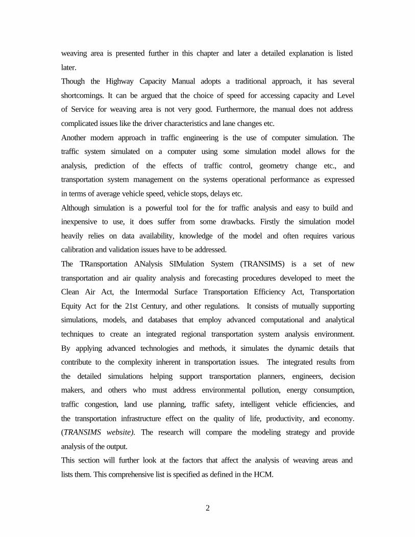
Type A Weaving Areas
These types of weaving areas require each weaving vehicle to make one lane change in
order to execute the desired movement. The Figure 1 shows two types of Type A
weaving areas. Shown in Figure 1a, is an on-ramp followed by an off-ramp, with a
continuous auxiliary lane between the ramps. In this configuration all on ramp vehicles
must perform one lane change out of the auxiliary lane into the shoulder lane of the
freeway, and all off-ramp vehicles must make a lane change from the shoulder lane of the
freeway to the auxiliary lane.
4
Figure 1a & b: Type A Weaving Sections (Source HCM)
These sections that are formed by on-ramp/off-ramp sequences joined by continuous
auxiliary lanes are referred to as ramp-weave sections. The Figure 1(b) shows a major
weaving section characterized by three or more entry and exit roadways having multiple
lanes. All weaving vehicles in this scenario too need to make at least one lane change to
get into their desired lanes.
This type of weaving configuration is characterized by the presence of a crown line (the
line connecting the nose of the entrance gore area to the nose of the exit gore area). Every
weaving vehicle makes a lane change and crosses over this crown line. The primary
difference between the two scenarios shown in the figure is the impact of ramp
geometrics on speed, the ramp weave model having its vehicle to accelerate or decelerate
as they move from the on to the off-ramp.
Since the weaving vehicles in this type of configuration cross the crown line, they are
usually confined to the two lanes adjacent to the crown line in the weaving section. A
significant effect of this configuration on operations is the maximum number of lanes that
weaving vehicles occupy while traversing the section.
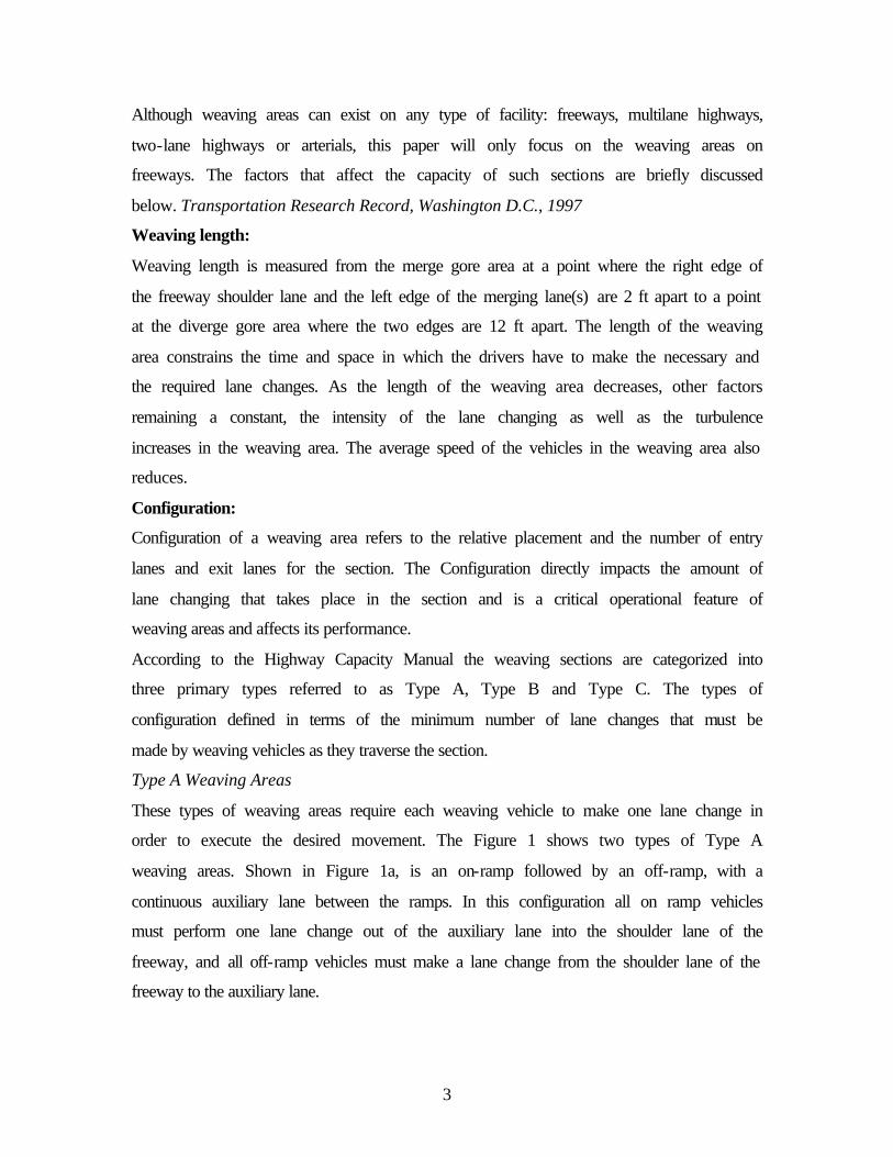
Type B Weaving Areas:
Type B configuration weaving areas involve multilane entry legs or exit legs or both.
Two characteristics that distinguish Type B with others are that one weaving movement
would not require any lane change while the other would require at most one lane change
for this configuration.
Figure 2 a, b and c shows three such weaving areas. As can be seen the movement B-C
would not require any lane changes while A-D would require one lane change. In Figure
2(a) it can be seen that this is achieved by lane balancing, while in b this is achieved by a
lane in Leg A merging with a lane from leg B at the entrance gore area.
( a ) ( b )
5
It has been found that this kind of a weaving configuration are efficient in carrying large
weaving volumes much attributed to the provision of a through lane from one weaving
movement. This configuration allows for the weaving vehicles to occupy a substantial
number of lanes in the weaving section and not restricted as in Type A configuration
sections.
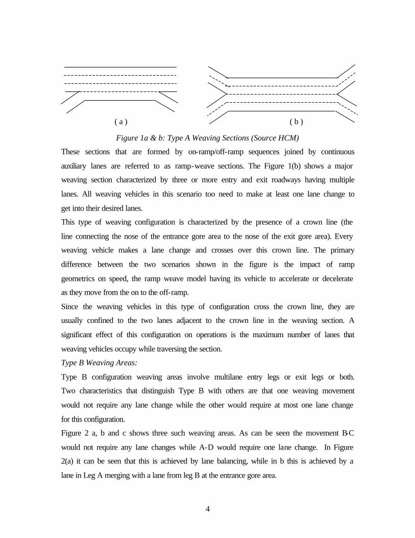
Type C Weaving Areas:
Type C configuration Weaving Areas are very similar to those of Type B. They are
similar in the fact that one weaving movement can be accomplished by no lane change
i.e., one or more through lanes are provided for one of the weaving movements. The
dissimilarity lies in the number of lane changes necessary for the other weaving
movement. A Type C weaving area is characterized by the fact that one weaving
movement can be accomplished without a lane change whilst the other weaving
movement requiring two or more lane changes. An example of this type of weaving
section is illustrated in the Figure 3.
It can be seen in the figure that the movement B-C does not require any lane change
while the movement A-D requires two lane changes which qualifies the section into a
Type C configuration weaving area.
Figure 2: Type B Weaving Sections (Source HCM)
( a ) ( b )
( c )
A
B
C
D
6
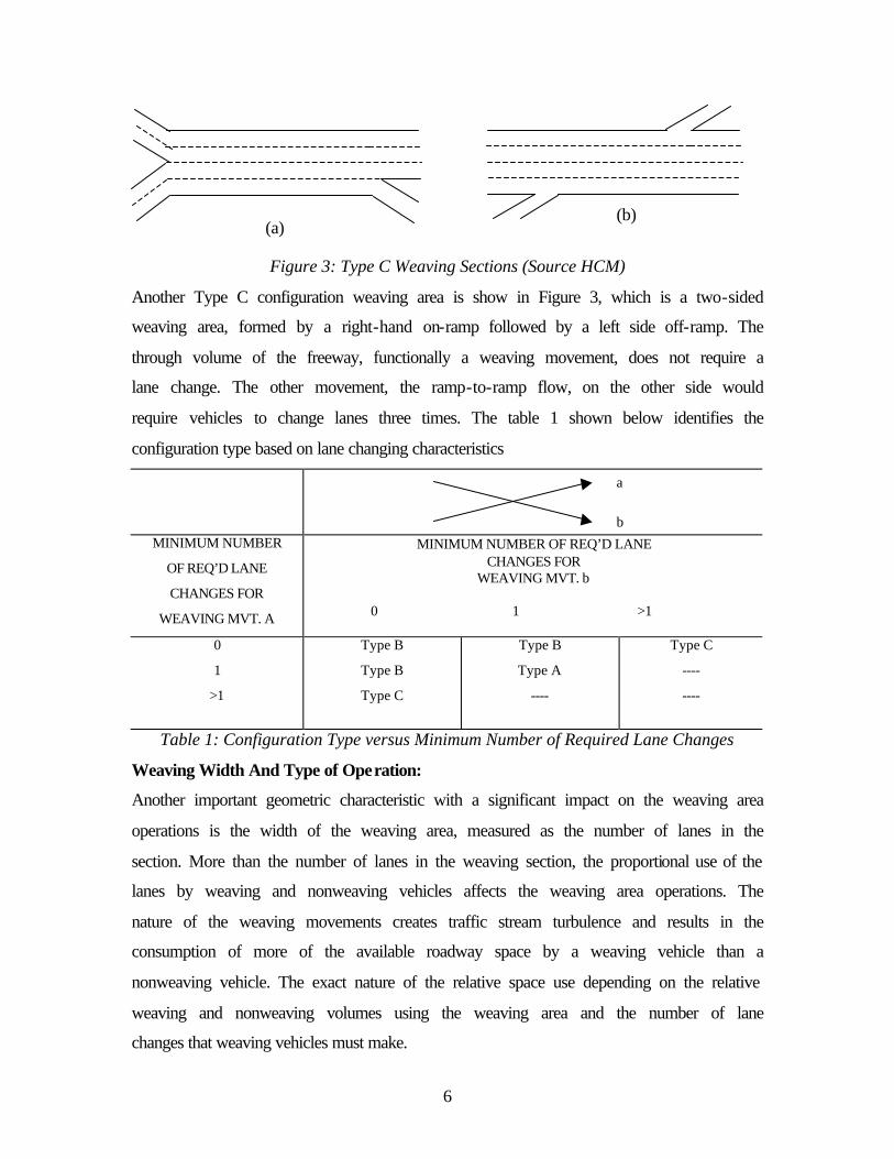
Figure 3: Type C Weaving Sections (Source HCM)
Another Type C configuration weaving area is show in Figure 3, which is a two-sided
weaving area, formed by a right-hand on-ramp followed by a left side off-ramp. The
through volume of the freeway, functionally a weaving movement, does not require a
lane change. The other movement, the ramp-to-ramp flow, on the other side would
require vehicles to change lanes three times. The table 1 shown below identifies the
configuration type based on lane changing characteristics
MINIMUM NUMBER
OF REQ’D LANE
CHANGES FOR
WEAVING MVT. A
MINIMUM NUMBER OF REQ’D LANE CHANGES FOR
WEAVING MVT. b 0 1 >1
0
1
>1
Type B
Type B
Type C
Type B
Type A
----
Type C
----
----
Table 1: Configuration Type versus Minimum Number of Required Lane Changes
Weaving Width And Type of Operation:
Another important geometric characteristic with a significant impact on the weaving area
operations is the width of the weaving area, measured as the number of lanes in the
section. More than the number of lanes in the weaving section, the proportional use of the
lanes by weaving and nonweaving vehicles affects the weaving area operations. The
nature of the weaving movements creates traffic stream turbulence and results in the
consumption of more of the available roadway space by a weaving vehicle than a
nonweaving vehicle. The exact nature of the relative space use depending on the relative
weaving and nonweaving volumes using the weaving area and the number of lane
changes that weaving vehicles must make.
a
b
(a) (b)

7
The impact of configuration is felt most in Type A sections where all weaving vehicles
must cross a crown line and is the least severe in Type B sections. It is also observed that
vehicles in the weaving area will make use of the available lanes in a way such that all
component flows achieve approximately the same average running speeds, with weaving
flows somewhat slower than nonweaving flows. Sometimes, the configuration type limits
the ability of weaving vehicles to occupy the proportion of available lanes required to
achieve this equivalent or balanced operation. Weaving vehicles in such cases occupy a
smaller proportion of the available lanes than desired, and nonweaving vehicles occupy a
larger proportion of lanes than for balanced operation. When this occurs, the operation of
the weaving area is classified as constrained by the configuration. The result of the
constrained operation is that nonweaving vehicles will operate at significantly higher
speeds than nonweaving vehicles.
Weaving Area Parameters
Table 2, shown below summarizes the parameters that may affect the operation of the
weaving areas and defines symbols that used to depict them.
Symbol Definition
L Length of the Weaving area, in ft
LH Length of the Weaving area, in hundreds of ft.
N Total number of lanes in the weaving area.
Nw Number of lanes used by weaving vehicles in weaving area.
Nnw Number of lanes used by nonweaving vehicles in weaving area.
V Total flow rate in weaving area, in passenger car equivalents, in pcph.
vw Total weaving flow rate in the weaving area, in passenger car equivalents, in pcph.
vw1 Weaving flow rate for the larger of the two flow rates, in passenger car equivalents, in pcph.
vw2 Weaving flow rate for the smaller of the two flow rates, in passenger car equivalents, in pcph.
vnw Total nonweaving flow rate in the weaving area, in passenger car equivalents, in pcph.
VR Volume ratio vw/v .
R Weaving ratio vw2/vw.
Sw Average (space mean) speed of weaving vehicles in the weaving area, in mph.
Snw Average (space mean) speed of nonweaving vehicles in the weaving area, in mph.
Table 2: Parameters Affecting Weaving Area Operation

8
1.3 Objective
The HCM has been developed on empirical data with certain assumptions while
TRANSIMS takes a different perspective to dealing with the handling of movements of
vehicles on the network. The objective of this study is to compare the TRANSIMS
weaving movements and results to that of HCM results. Scenarios already existing in the
HCM are modeled using TRANSIMS. Type A Weaving areas are only tested in both
cases as they are the most common type facilities found on freeways. The factors that
affect the speed of the vehicles in the weaving section and thus the density are identified.
A comparative study of the two models in accessing the freeway sections is conducted.
The limitations of each model are described and finally possible recommendations are
made to both TRANSIMS for future research.
1.4 Organization of the Thesis
In Chapter 2, a literature review is presented on all the past research conducted in this
area. Ongoing research in this area is also discussed here. Chapter 2 also discusses the
various ways in which vehicular traffic theory has been modeled highlighting the
advantages and the drawbacks of each theory.
Chapter 3 describes the methodologies used by HCM and TRANSIMS. Procedure for
application is also given for the HCM. A brief discussion of TRANSIMS package
highlighting the Microsimulator is presented.
This is followed by the description of the proposed research in Chapter 4. The scenarios
that are compared, analyzed and modeled are described. The modeling strategies adopted
to model these scenarios are also discussed.
The comparison and sensitivity analysis of results are presented in Chapter 5. Also
included in the chapter are the recommendations for future research.
The data used for analysis and validation form the Appendix A. Appendix B contains the
data used for plotting various graphs in this paper.
9
Chapter 2: Literature Review
2.1 Introduction
In this chapter, the literature behind weaving analysis is discussed. Since the scope of this
research is to provide a comparative analysis between HCM and TRANSIMS for
weaving highway sections, various factors such as speed, capacity of the freeway etc.
affecting weaving operation is briefly outlined. Since TRANSIMS is essentially a particle
hopping cellular automata model. This type of model is described here. Further for the
better understanding of the various ways of representing vehicular traffic in a simulation
modeling environment, the various approaches such as fluid mechanical models and car
following models are described too. The various analytical models, which led to the
development of the current version of the simulation model are discussed. This chapter
also talks about the advantages and disadvantages of using a computer model versus an
analytical model.
2.2 Past Research Related to Freeway Weaving Analysis
The methodology adopted in the comparative analysis is to model a particular weaving
scenario using both HCM and TRANSIMS. To adjust the simulation model, various
factors such as capacity of the weaving section, speed, driver characteristics etc needs to
be studied. As the scope of my research is to identify various parameters, which affect the
result of simulation and methods to improve them, the next few paragraphs talk about
some earlier research done on some of the various parameters, which might affect the
calibration of the model and their resulting conclusions. Suresh Ramachandran et al.
A study on capacity and level of service at ramp freeway junctions by Roger P. Roess
and Jose M. Ulerio found that if some parameters such as volume distribution, speed
variance can be improved, its use could augment field data and allow more consistent and
thorough calibration of regression/simulation models. The importance of the driver
population to the freeway traffic operation analysis also should not be neglected. In
analyzing freeway capacity, one of the most important factors is speed because service
flow rate can be obtained from the value of density multiplied by the value of average
speed. Most traditional weaving analysis methods use roadway geometry and traffic
10
volumes as inputs and provide an estimate of speed as an output. The use of speed for
assessing the capacity and level of service for weaving has proved to be a poor choice.
One reason is that speed is not very sensitive to flow at saturation level. A study
conducted by Halati et al has shown that the concept of a stable relationship between
speed and flow is fundamentally flawed. As flow nears capacity, it begins a series of fast
and unstable jumps from the smooth flow to an unstable one. With this approach, traffic
only flows at capacity speed while transitioning from fast sub capacity flow to a slow
congested flow. In effect, capacity speed is ephemeral and can be quantified in averages.
Since speed has been identified as one of the important factors that might affect the
calibration of the model, the variance of speed in the output results needs to be studied.
The next few paragraphs talk about the impact of speed limit on a freeway. A study
conducted by Jack D. Jernigan and Cheryl W. Lynn on impact of speed limit on freeway
showed that the speed limit has influence on average speed, percentile speed and speed
variation. According to their study for Virginia’s rural interstate highway, they indicated
that the average speed of Virginia’s rural interstate was 56.3 mph when the speed limit
was 55 mph and the percentile speed was 62mph. One year after the speed limit was
increased to 65mph the average speed was 63.5mph and the percentile speed was 70mph.
In another study, Harkey, David L., Robertson, Douglas, and Davis, Scott E., found that
an increase of 4mph occurred in percentile speed of the passenger vehicles along the rural
interstate highways in Illinois after the change of the 65mph speed limit from 55 mph
speed limit. Nicholas J. Garber and Ravi Gadijaru conducted a study on factors affecting
speed variance. They found that the difference between the design speed and the posted
speed limit had a statistically significant effect on speed variance. Furthermore they
found that drivers tend to drive at increasing speeds as the roadway geometrics improved,
regardless of the posted speed limits.
Another study was conducted by Adolph D. May, to determine the congestion causes in
weaving areas. One of the important observations that came out from this research was
that vehicles tend to reduce speed in weaving areas depending upon the merging
characteristics of the driver, number of lanes and volume distribution. These observations
were made were based on several factors such as interrelationships between volume,
occupancy and speed, the measurement of the effect of congestion on traffic flow and
11
travel time and a comparison of traffic characteristics just before and after congestion
Essam Radwan and Sylvester A. F. Kalevela conducted an investigation of the effect of
change in vehicular characteristics on the highway capacity. The results from analyzing
traffic flow models and time headway’s showed that despite the change in vehicular
characteristics there has not been a discernible corresponding change in highway
parameters. This research clearly shows that by altering various vehicular parameters,
there has been no influence on highway parameters.
2.3 Vehicular Traffic Theory
Vehicular traffic theory has traditionally been modeled in different ways, which can
broadly be classified into three groups: Traffic flow model, car-following model and
particle hopping model.
Particle Hopping Models
Another approach for modeling traffic is the use of particle hopping model. In general all
particle-hopping models are defined on a lattice. The lattice being made up of a certain
number of sites, each of which an either is empty or occupied by a particle. Another
characteristic of the model is that only one particle can occupy each site and all the
movement of these particles is to be in one direction. This model adheres to the laws of
conservation of total mass, which states that the total particles in the system are
conserved except at boundaries where particles can either enter or exit. In traffic models
the road segments are generally thought of as a lattice and each vehicle represents
particles. (Nagel, K. et al, LA-UR 96-659)
The Stochastic Traffic Cellular Automaton (STCA)
The characteristics of the Stochastic Traffic Cellular Automaton are defined below. Each
particle (in traffic sense referring to a vehicle) has a velocity that is either 0 or an integer.
The speed constrained by a maximum of vmax. This means that every vehicle can only
take integer values of velocity between 0 and vmax. The configuration of timestep t+1 is
computed from the stored configuration of timestep t, using either parallel or
synchronous updates. The decisions for the timestep t+1 entirely depend on the
configuration at timestep t. Briefed below are the update procedures executed by every
particle/vehicle in parallel. (Nagel,K. et al, LA-UR 95-2098)
12
• The gap ahead of the particle/vehicle is computed
• If the velocity of the particle is greater than the gap,
a need for slowing down the particle is observed and its velocity changed
so it equals the gap ahead.
Else if there is enough headway in front of the vehicle and the vehicle is not
moving at the maximum speed allowed then
its velocity is incremented so as to represent and acceleration. This
acceleration is however gradual so as to represent daily behavior.
• To capture the realistic behavior of traffic, some randomness is introduced. This
models the idea of particles/vehicles slowing down without reason, fluctuations at
maximum speed, overreactions at breaking and noisy accelerations. For such a
condition to occur, the velocity of the particle should clearly be positive and non-
zero. With a probability p, the velocity of such a particle is thus reduced by one.
• Once these decisions have been taken the particle/vehicle is moved ahead
depending on the velocity computed as listed above.
It is interesting to note in this model if the maximum velocity is set to one, i.e., vmax =1,
then the model behaves very differently from what it would when the maximum velocity
is greater than two. All the conditions stated above reduce to a singular statement that
states a particle to move ahead to the next cell with a probability of p, should it be free.
The analysis for STCA/2 (STCA with vmax>=2) shows that there is a very dynamic and a
different flow regime that does not have an exact solution. Inspection of the space-time
plots visually confirmed that the dynamics of this model was very similar to STCA-CC/2
(which is discussed later) more than to the ASEP (discussed later). It was observed that
multiple jams could exist simultaneously. Jams in such a models start simultaneously and
independently of other jams attributed to the velocity fluctuations at maximum speed and
depended on the parameter pfree (not equal to zero).
2.3.1.1 The Cruise Control Limit of STCA (STCA-CC)
This model is very similar to the one described previously. The difference being in the
way fluctuations occur at free driving speeds i.e., at maximum speed and undisturbed by
other cars. The fluctuations at these cruise speeds are set to zero. All the rules for
13
particles/vehicles not traveling at maximum speeds remain the same as that of STCA
discussed in the previous subsection. (Nagel,K. et al, LA-UR 95-2098)
A new set of rules that all particles/vehicles do in parallel is listed below.
• Should a vehicle be traveling at maximum velocity vmax and there be free
headway i.e., gap greater than or equal to vmax, then the vehicle maintains its
velocity.
• Else (i.e., vehicle not at maximum velocity or no free headway) the standard rules
1-3 of Stochastic Traffic Cellular Automaton are applied.
The analysis of STCA-CC/1 clearly shows that the maximum flow occurs with all cars at
maximum speed and having ahead of them a gap greater than or equal to the maximum
velocity. When the density of flow is less than the density of the maximum flow of the
deterministic model. ρc2 = 1 / ( vmax + 1 ), the flow is smooth. It is also seen that above a
certain density ρc1 the flow becomes unstable to local perturbations. When a perturbed
car slows down and eventually re-accelerates to the maximum velocity, the following car
might have come too close to it and has to break/slow down. This may initiate a chain
reaction and thus an emergent traffic jam.
The STCA-CC/2 with a maximum velocity greater than or equal to two is seen not to
have changed the critical behavior described above but add a complication. Jam clusters
are seen to branch, with large jam-free holes between branches of jams. The space-time
graphs of such flows appear to show fractal properties.
2.3.1.2 The Deterministic Limit of the STCA (CA-184)
The deterministic limit of the STCA models unprobabilistic nature of the STCA i.e.,
taking the randomness out of the randomness step. This is, when the maximum velocity
equal to one, equivalent to cellular automaton rule 184 in wolfram’s notation. (Nagel,K.
et al, LA-UR 95-2098) It is interesting to note that most Cellular Automaton Traffic
models are based on this model.
14
2.3.1.3 The Cruise Control version of CA-184 (CA-184-CC)
This is a different CA model that is equivalent to the deterministic cruise control situation
for the CA-184/1. If the maximum velocity considered is vmax = 1, the rules are simple
and short and are described below.
All particles follow this set of rules in parallel
• If velocity is equal to one and the site ahead is free or the gap is greater than one
then the particle/vehicle is moved onto the next cell
• If the velocity of the particle is zero or in other words the particle is at rest then it
cannot move until the gap ahead is greater than or equal to two cells.
Although the rule set has been detailed for a maximum velocity of one, generalizations to
this model where the maximum velocities are greater than one are straightforward.
2.3.1.4 The Asymmetric Stochastic Exclusion Process (ASEP)
The Asymmetric Exclusion Process or ASEP for short is probably the most investigated
particle-hopping model. The ASEP models behavior that can be generalized by two
simple rules stated below
• Selection of a random particle/vehicle;
• Movement of the particle to the right should the space on that site be empty.
The ASEP model is closely related to the STCA and CA models that were discussed
earlier. The ASEP model behaves just the same way that STCA/1 and CA-184/1 do. This
is because in rule two of ASEP, particles are only updated to the next site and not further.
The basic difference though between them would be the way in which the particles are
updated.
STCA/1 and CA-184/1 particles are all updated once and synchronously while ASEP
does random updates of particles in a sense that these updates are a random serial
sequence. However comparisons can be made between these models after defining the
quantity timestep for the ASEP model. The definition of a timestep is clear and
understood for the STCA and the CA-184 models as being the time between two
successive updates of particles. In ASEP at an average a particle is updated after n single-
particle updates, a timestep is thus completed after N single-particle updates.
It can also be observed that the randomness in the updates of the particles can be reduced
i.e., reduction in the noise by techniques discussed by Wolf and Kertesz. They stated that
15
using a counter associated with every particle could considerably reduce the noise if the
updates are only made after k trials. It can also be seen that as k increases to a very large
value the ASEP model slowly tends to behave as a CA-184. (Nagel,K. et al, LA-UR 95-
2098)
2.3.2 Traffic Flow Theory – (Fluid Dynamical Models)
This kind of a modeling typically involves the identification of relations between the
three fundamental variables of traffic flow namely velocity (v), density (ρ) and flow (j).
Of the three variables, two are considered independent and the following relation exists
among the three; j=ρν. The possible units for the three variables being [ν] = km/hr, [ρ]=
veh/km and [j]= veh/hr.
The type of an approach originated from the conventional fluid-dynamical models. The
theory being developed from the standard fluid-dynamical conservation equations for
mass and momentum as a beginning point, which are stated below.
∂t ρ + ∂x (ρν) = 0 (equation of continuity) …...(2.1)
dv/dt = ∂t ν + ν. ∂x ν = F/m ( momentum equation) …...(2.2)
Where
ρ is the density;
ν is the velocity;
d/dt is the individual derivative (Lagrangian);
F is the force acting on a mass m.
The first equation capturing the mass conservation while the second equation describes
the fact that momentum of mass m changes only due to a force F. The force F in traffic
terms would include vehicle and individual driving dynamics. (Nagel,K. et al, LA-UR 95-
4018)
Described below are the improvements and additions to the basic continuity equation or
other approaches developed from these basic equations. Each of them is highlighted
below and described in brief (Nagel,K. et al, LA-UR 95-2908), but in enough detail to
give continuity and meaning to the following chapters.
16
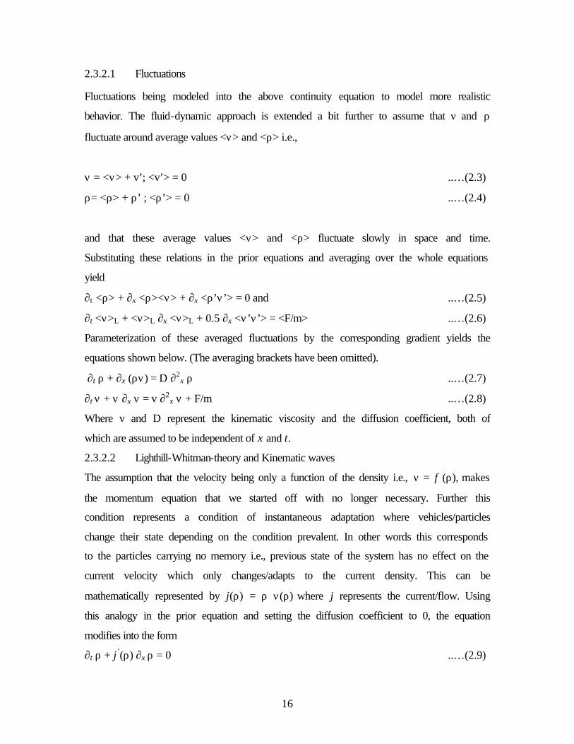
2.3.2.1 Fluctuations
Fluctuations being modeled into the above continuity equation to model more realistic
behavior. The fluid-dynamic approach is extended a bit further to assume that ν and ρ
fluctuate around average values <ν> and <ρ> i.e.,
ν = <ν> + v’; <v’> = 0 ..…(2.3)
ρ= <ρ> + ρ’ ; <ρ’> = 0 ..…(2.4)
and that these average values <ν> and <ρ> fluctuate slowly in space and time.
Substituting these relations in the prior equations and averaging over the whole equations
yield
∂t <ρ> + ∂x <ρ><ν> + ∂x <ρ’ν’> = 0 and ..…(2.5)
∂t <ν>L + <ν>L ∂x <ν>L + 0.5 ∂x <ν’ν’> = <F/m> ..…(2.6)
Parameterization of these averaged fluctuations by the corresponding gradient yields the
equations shown below. (The averaging brackets have been omitted).
∂t ρ + ∂x (ρν) = D ∂2x ρ ..…(2.7)
∂t ν + ν ∂x ν = v ∂2x ν + F/m ..…(2.8)
Where v and D represent the kinematic viscosity and the diffusion coefficient, both of
which are assumed to be independent of x and t.
2.3.2.2 Lighthill-Whitman-theory and Kinematic waves
The assumption that the velocity being only a function of the density i.e., ν = f (ρ), makes
the momentum equation that we started off with no longer necessary. Further this
condition represents a condition of instantaneous adaptation where vehicles/particles
change their state depending on the condition prevalent. In other words this corresponds
to the particles carrying no memory i.e., previous state of the system has no effect on the
current velocity which only changes/adapts to the current density. This can be
mathematically represented by j(ρ) = ρ ν(ρ) where j represents the current/flow. Using
this analogy in the prior equation and setting the diffusion coefficient to 0, the equation
modifies into the form
∂t ρ + j’(ρ) ∂x ρ = 0 ..…(2.9)
17
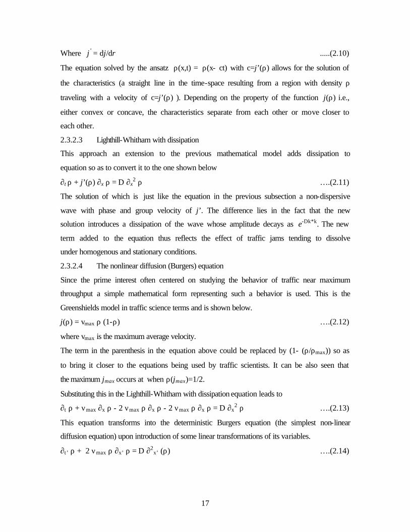
Where j’ = dj/dρ .....(2.10)
The equation solved by the ansatz ρ(x,t) = ρ(x- ct) with c=j’(ρ) allows for the solution of
the characteristics (a straight line in the time-space resulting from a region with density ρ
traveling with a velocity of c=j’(ρ) ). Depending on the property of the function j(ρ) i.e.,
either convex or concave, the characteristics separate from each other or move closer to
each other.
2.3.2.3 Lighthill-Whitham with dissipation
This approach an extension to the previous mathematical model adds dissipation to
equation so as to convert it to the one shown below
∂t ρ + j’(ρ) ∂x ρ = D ∂x2 ρ ….(2.11)
The solution of which is just like the equation in the previous subsection a non-dispersive
wave with phase and group velocity of j’. The difference lies in the fact that the new
solution introduces a dissipation of the wave whose amplitude decays as e-Dk*k. The new
term added to the equation thus reflects the effect of traffic jams tending to dissolve
under homogenous and stationary conditions.
2.3.2.4 The nonlinear diffusion (Burgers) equation
Since the prime interest often centered on studying the behavior of traffic near maximum
throughput a simple mathematical form representing such a behavior is used. This is the
Greenshields model in traffic science terms and is shown below.
j(ρ) = vmax ρ (1-ρ) ….(2.12)
where vmax is the maximum average velocity.
The term in the parenthesis in the equation above could be replaced by (1- (ρ/ρmax)) so as
to bring it closer to the equations being used by traffic scientists. It can be also seen that
the maximum jmax occurs at when ρ(jmax)=1/2.
Substituting this in the Lighthill-Whitham with dissipation equation leads to
∂t ρ + νmax ∂x ρ - 2 νmax ρ ∂x ρ - 2 νmax ρ ∂x ρ = D ∂x2 ρ ….(2.13)
This equation transforms into the deterministic Burgers equation (the simplest non-linear
diffusion equation) upon introduction of some linear transformations of its variables.
∂t ’ ρ + 2 νmax ρ ∂x’ ρ = D ∂2x’ (ρ) ….(2.14)
18
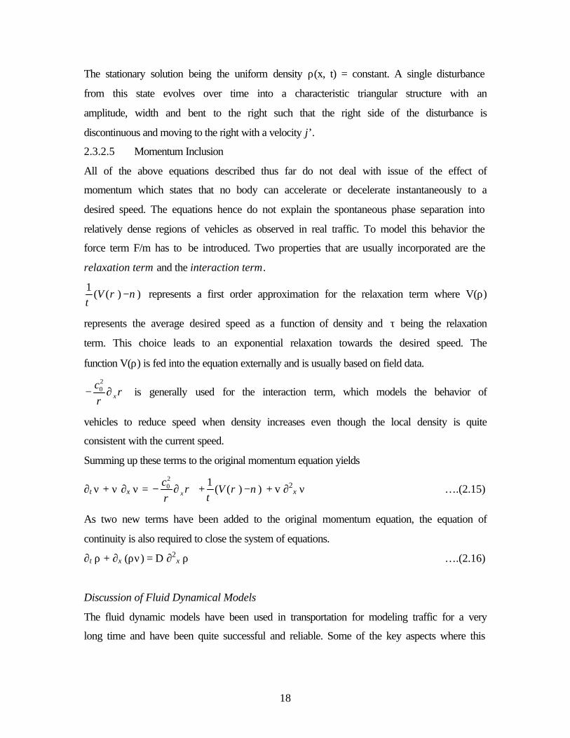
The stationary solution being the uniform density ρ(x, t) = constant. A single disturbance
from this state evolves over time into a characteristic triangular structure with an
amplitude, width and bent to the right such that the right side of the disturbance is
discontinuous and moving to the right with a velocity j’.
2.3.2.5 Momentum Inclusion
All of the above equations described thus far do not deal with issue of the effect of
momentum which states that no body can accelerate or decelerate instantaneously to a
desired speed. The equations hence do not explain the spontaneous phase separation into
relatively dense regions of vehicles as observed in real traffic. To model this behavior the
force term F/m has to be introduced. Two properties that are usually incorporated are the
relaxation term and the interaction term.
))((1
νρτ
−V represents a first order approximation for the relaxation term where V(ρ)
represents the average desired speed as a function of density and τ being the relaxation
term. This choice leads to an exponential relaxation towards the desired speed. The
function V(ρ) is fed into the equation externally and is usually based on field data.
ρρ xc
∂−20 is generally used for the interaction term, which models the behavior of
vehicles to reduce speed when density increases even though the local density is quite
consistent with the current speed.
Summing up these terms to the original momentum equation yields
∂t ν + ν ∂x ν = ρρ xc
∂−20 + ))((
1νρ
τ−V + v ∂2
x ν ….(2.15)
As two new terms have been added to the original momentum equation, the equation of
continuity is also required to close the system of equations.
∂t ρ + ∂x (ρν) = D ∂2x ρ ….(2.16)
Discussion of Fluid Dynamical Models
The fluid dynamic models have been used in transportation for modeling traffic for a very
long time and have been quite successful and reliable. Some of the key aspects where this
19
theory does not perform well are listed below. The listing is though not comprehensive
provides enough insight and identifies key areas where the model does not do well.
One of the major unsettling issues associated theory is that the relation between two of
the variables has to be fed into the model i.e., the relation between speed or flow and
density. This means the theory developed might eventually be different for different
interpretations of these relations and would differ fundamentally. The fact that there is no
common standpoint on the functional form of the speed-density relation further
complicates the issue.
Another problem area lies in the fact that the fluid dynamical models deal with
fluids/gases where an increase in the temperature would result in the increase in the
random fluctuations of particles about their mean. This implies that for gasses the
fluctuations and temperature increase with density, while in our case granular media i.e.,
vehicular traffic these fluctuations are observed to decrease with density (inside a jam)
and this inverse temperature effect is claimed to be responsible for clustering. (Nagel,K.
et al, LA-UR 95-4018)
Another point of contention voiced by some is the claim that all second-order fluid
dynamical models produce unrealistic behavior (such as backwards moving vehicles
caused by the diffusion term) making it unsuitable for modeling of traffic streams.
2.3.3 Car Following Model
The car following model for studying traffic behavior models traffic based on individual
car reactions. This type of modeling traffic is classified as microscopic because of its
nature of handling the movements of vehicles and resolution. Every vehicle makes a
decision depending on parameters of the leading vehicle and its own characteristics. It
should be noted that the macroscopic characteristics such as the flow, density etc., are all
aggregated from these individual vehicle interactions. This type of an analysis of the
system allows for the close inspection of individual behavior of vehicles or allows for the
rules to be written so as to model individual behavior rather than a wholistic view of the
system variables in the form of equations as done by the macroscopic variables.
This subsection will focus on the various car-following models that are in use and briefly
explain some algorithms developed over the years. A characteristic about the car
following approach is the way in which all of the models model the behavior of each
20
vehicle in relation to the vehicle ahead. It should also kept in mind that this theory is
mainly accurate for single lane situations where in reality every driver reacts only to the
vehicle in front of him/her. Most of the car following models use the equation of the form
given below for interaction between the vehicle and the leading car. (Suresh
Ramachandran et al.)
)(.)]([
v(t) )(
m
tvtx
Ttal
∆∆
+ α ….(2.17)
Where
a represents the acceleration of the car under consideration;
v represents the velocity of the car under consideration;
∆x represents distance of the two vehicles; (car under observation and leading vehicle)
∆v is the velocity difference between the car under observation and the leading vehicle;
T represents the delay time between stimulus and the response time; and
m and l being constants.
Other forms of the equation also are in use to model car following but generally having
an equation that relates the acceleration of the vehicle under observation to the velocity
difference and the space between the vehicles. Mathematically, parts of this theory are
very similar to the treatment of atomic movements in crystals, and gives results about the
stability of chains of cars (“platoons”) in following-the-leader situation. These car
following models were successful in a way that they could model the static flow-density
relations that were observed to some extent.
For use in digital micro simulations, the analytical car-following models described above
are seen to have two drawbacks, firstly they are developed for a continuous rather than
discrete time parameter and secondly no single model would be appropriate to all traffic
conditions. As a result traffic simulation models have been developed and deployed.
Fail safe models is a process of determining a vehicles speed and position given that its
leader has a speed and position that has already been calculated, for the current time span.
Such a type of model has two elements, 1) there is a car-following model which
calculates the followers’ behavior based on some prescribed following distance and 2) the
21
model has an overriding collision factor which prevents the following vehicle to avoid
collision when the leader undergoes extreme deceleration pattern. Three Algorithms are
considered here and looked into in detail.
2.3.3.1 The UTCS-1 Algorithm:
This model consists of a spacing algorithm, which provides for collision avoidance when
the leading vehicle decelerates suddenly to a stop. There is no specific car-following
algorithm apart from the critical headway calculations. The output of the algorithm, is
given by
A=[7(x-y-vT-L)+(2u2-3v2)/6]/(v+3) ….(2.18)
where
a = acceleration of the follower
x = position of the leader
y = position of the follower
u = speed of the Leader
v = speed of the follower
L = length of the leader
T = simulation scanning interval.
2.3.3.2 The Aerospace Algorithm
This model uses the May-Keller calibration of the conventional analytical car-following
model
A=λy(u-v)/(x-y)2 ….(2.19)
where λ is the driver sensitivity factor.
When (u-v) is positive or close to zero, the above formula is inoperative and
normal acceleration patterns are followed subject to safe spacing limitations.
2.3.3.3 The PITT Algorithm:
The PITT algorithm was developed by the university of Pittsburgh. This model is
founded on a combination of the Northwestern car following and the UTCS collision
avoidance features. The primary car following relationship is that a following vehicle
attempts to maintain a space headway of L+kv+10+bk(u-v)2 feet. The sensitivity factor,
“k”, which is a function of driver type, regulates maximum lane capacity. The car
following formula is
22
A=2[x-y-L-10-(k+T)v – bk(u-v)2]/(T2 + 2kT) ….(2.20)
where
b = constant for high relative closing speed
A lag, c, is introduced into this formula after ‘a’ has been calculated. The lag is applied to
the speed and new speed is calculated as follows
v1 = v+ a(T-c) ….(2.21)
Overriding this car following model is a collision avoidance set of equations that prevent
collisions when vehicles are undertaking maximum emergency deceleration.
These collision avoidance equations are constraints, which determine the follower
vehicles acceleration, which must be maintained in order to satisfy emergency non –
collision conditions. The emergency constraint is also used in lane changing mechanism
where vehicles may not be in a safe position relative to each other.
2.4 Simulation
Simulation modeling is a tool often used for analyzing a wide variety of dynamical
problems, which are not amenable to study by other means. Such problems, usually
associated with complex processes, cannot be readily described in analytical terms. They
are generally characterized by the interaction of many system components or entities.
The behavior of each entity and the interaction of a limited number of entities, being well
understood and which can be reliably represented logically and mathematically with
acceptable confidence. However, the complex, simultaneous interactions of many system
components cannot be adequately described in mathematical or logical forms.
Simulation models are designed to "mimic" the behavior of such systems. The simulation
models integrate these separate entity behaviors and interactions to produce a detailed,
quantitative description of system performance. The simulation models are
mathematical/logical representations (or abstractions) of real-world systems, which take
the form of software executed on a digital computer in an experimental fashion. The
results usually numeric provide the analyst with detailed quantitative descriptions of what
is likely to happen in such a real world scenario. The graphical and animated
representations of the system functions provide insights so that the trained observer can
23
gain an understanding of why the system is behaving this way. The proper interpretation
of the results from the wealth of information provided by the model helps in gaining an
understanding of cause-and-effect relationships.
Almost all traffic simulation models describe dynamical systems where time is always the
basic independent variable. This section further highlights the categories into which
simulation models are classified.
Continuous simulation models describe how the elements of a system change state
continuously over time in response to continuous stimuli whereas Discrete simulation
models represent real-world systems (that are either continuous or discrete) by asserting
that their states change abruptly at points in time. There are generally two types of
discrete models: a) Discrete time and b) Discrete event. The first, segments time into a
succession of known time intervals. Within each such interval, the simulation model
computes the activities, which change the states of selected system elements. This
approach is analogous to representing an initial-value differential equation in the form of
a finite-difference expression with the independent variable, t.
Some systems are characterized by entities that are "idle" much of the time. For such
systems of limited size or those representing entities whose states change infrequently,
discrete event simulations are more appropriate than are discrete time simulation models,
and are far more economical in execution time. However, for systems where most entities
experience a continuous change in state (e.g., a traffic environment) and where the model
objectives require very detailed descriptions, the discrete time model is a better choice.
Simulation models may also be classified according to the level of detail with which they
represent the system to be studied:
• Microscopic (high fidelity)
• Mesoscopic (mixed fidelity)
• Macroscopic (low fidelity)
A microscopic model describes both the system entities and their interactions at a high
level of detail. A mesoscopic model generally represents most entities at a high level of
detail but describes their activities and interactions at a much lower level of detail than
would a microscopic model. A macroscopic model describes entities and their activities
and interactions at a low level of detail.
24
High-fidelity microscopic models, and the resulting software, are costly to develop,
execute and to maintain, relative to the lower fidelity models. While these detailed
models possess the potential to be more accurate than their less detailed counterparts, this
potential may not always be realized due to the complexity of their logic and the larger
number of parameters that need to be calibrated.
Lower-fidelity models are easier and less costly to develop, execute and to maintain.
They carry a risk that their representation of the real-world system may be less accurate,
less valid or perhaps, inadequate. Use of lower-fidelity simulations is appropriate if:
• The results are not sensitive to microscopic details.
• The scale of the application cannot accommodate the higher execution time of the
microscopic model.
• The available model development time and resources are limited.
Another classification of the simulation models, which addresses the processes,
represented by the model: (1) Deterministic and (2) Stochastic.
Deterministic models have no random variables; all entity interactions are defined by
exact relationships (mathematical, statistical or logical). Stochastic models have
processes, which include probability functions. For example, a car-following model can
be formulated either as a deterministic or stochastic relationship by defining the driver's
reaction time as a constant value or as a random variable, respectively.
Since simulation models describe a dynamical process in statistical and pictorial formats,
they can be used to analyze a wide range of applications ranging from queuing problems
to scheduling tasks to optimal shipping strategies to wherever
• Mathematical treatment of a problem is infeasible or inadequate due to its temporal
or spatial scale, and/or the complexity of the traffic flow process.
• The assumptions underlying a mathematical formulation (e.g., a linear program) or a
heuristic procedure (e.g., those in the Highway Capacity Manual) cast some doubt on
the accuracy or applicability of the results.
• The mathematical formulation represents the dynamic traffic/control environment as
a simpler quasi steady-state system.
• There is a need to view vehicle animation displays to gain an understanding of how
the system is behaving in order to explain why the resulting statistics were produced.
25
• Congested conditions persist over a significant time.
It must be emphasized that traffic simulation, by itself, cannot be used in place of
optimization models, capacity estimation procedures, demand modeling activities and
design practices. Simulation can be used to support such undertakings, either as
embedded submodels or as an auxiliary tool to evaluate and extend the results provided
by other procedures.
2.4.1 CORSIM (Microscopic) Vs TRANSIMS (Mesoscopic)
Before discussing the different methodologies adopted by TRANSIMS and Highway
Capacity Manual a brief summary of the differences between two existing simulation
models is presented here. The reason for the choice of CORSIM (Corridor Simulation) is
its popularity in traffic simulation communities.
The first and the foremost striking difference is in basic nature of the models itself,
CORSIM represents a microscopic model where each vehicle is modeled individually
and whereas TRANSIMS is a mesoscopic simulation model with a trade-off between the
resolution and fidelity. Although the degree of detail in TRANSIMS is a single vehicle,
the location and speed of the vehicle suffers from some error. Although TRANSIMS
Microsimulator is a kind of car following model as vehicle movements occur based on
the gap ahead and the current velocity, it is not a true car-following model as the leader
cars’ velocity is not used in the calculations of the follower.
With reference to weaving sections the comparisons can be highlighted in the lane
changing logic. There are more microscopic parameters captured in the CORSIM model
in terms of maneuver time, percentage of co-operative drivers etc.
26
Chapter 3: Methodologies TRANSIMS and HCM
In this Chapter a detailed outline of how each of the models, HCM and TRANSIMS,
treats weaving models is outlined. Firstly the procedures in the Highway Capacity
Manual are discussed, following which the TRANSIMS procedures are shown. As
TRANSIMS has no separate logic in the handling of weaving maneuvers, the algorithm
of lane changing and movement of vehicles is discussed. The inputs to the
Microsimulator are also presented.
3.1 HCM Methodology
The four important steps in the analysis of weaving sections identified by the HCM
include the prediction of the weaving and nonweaving speeds, determination about the
type of weaving operation, a check to see if the analysis is within the limiting values
defined in the HCM and finally the estimation of the Level of Service after the
calculation of the average density of the weaving area. Transportation Research Record,
Washington D.C., 1997
Prediction of Weaving and Nonweaving Speeds:
A very important step in the analysis of weaving areas is the prediction of speeds and
density of vehicles within the weaving area. As can be understood, the speeds of weaving
and nonweaving vehicles can vary largely and hence are predicted separately. Finally an
average speed and density is estimated for all the vehicles, the level of service determined
based on the density.
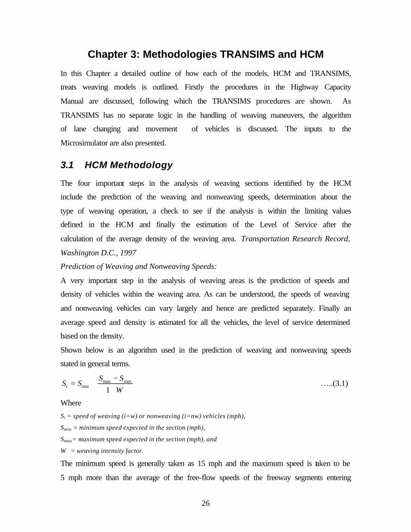
Shown below is an algorithm used in the prediction of weaving and nonweaving speeds
stated in general terms.
WSS
SSi +−
+=1
minmaxmin …..(3.1)
Where
Si = speed of weaving (i=w) or nonweaving (i=nw) vehicles (mph),
Smin = minimum speed expected in the section (mph),
Smax= maximum speed expected in the section (mph), and
W = weaving intensity factor.
The minimum speed is generally taken as 15 mph and the maximum speed is taken to be
5 mph more than the average of the free-flow speeds of the freeway segments entering
27
and leaving the section. The addition of the 5 mph accounts for the underpredicton of
high speeds. The new equation would then be represented as
WS
S FFi +
−+=
110
15 Where, …..(3.2)
SFF = average free flow speed of the freeway segments entering and leaving the weaving area
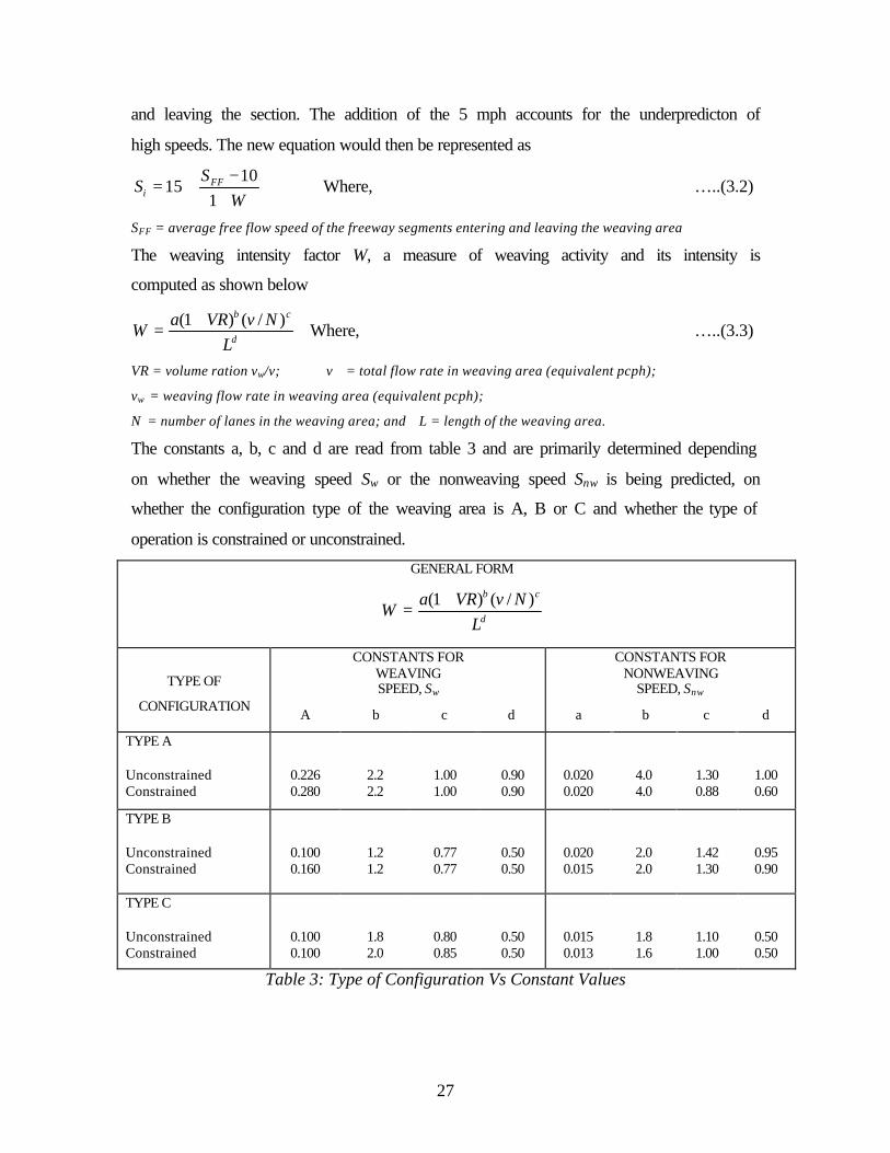
The weaving intensity factor W, a measure of weaving activity and its intensity is
computed as shown below
d
cb
LNvVRa
W)/()1( +
= Where, …..(3.3)
VR = volume ration vw/v; v = total flow rate in weaving area (equivalent pcph);
vw = weaving flow rate in weaving area (equivalent pcph);
N = number of lanes in the weaving area; and L = length of the weaving area.
The constants a, b, c and d are read from table 3 and are primarily determined depending
on whether the weaving speed Sw or the nonweaving speed Snw is being predicted, on
whether the configuration type of the weaving area is A, B or C and whether the type of
operation is constrained or unconstrained.
GENERAL FORM
d
cb
LNvVRa
W)/()1( +
=
CONSTANTS FOR WEAVING SPEED, Sw
CONSTANTS FOR NONWEAVING
SPEED, Snw
TYPE OF
CONFIGURATION A b c d a b c d
TYPE A Unconstrained Constrained
0.226 0.280
2.2 2.2
1.00 1.00
0.90 0.90
0.020 0.020
4.0 4.0
1.30 0.88
1.00 0.60
TYPE B Unconstrained Constrained
0.100 0.160
1.2 1.2
0.77 0.77
0.50 0.50
0.020 0.015
2.0 2.0
1.42 1.30
0.95 0.90
TYPE C Unconstrained Constrained
0.100 0.100
1.8 2.0
0.80 0.85
0.50 0.50
0.015 0.013
1.8 1.6
1.10 1.00
0.50 0.50
Table 3: Type of Configuration Vs Constant Values
28
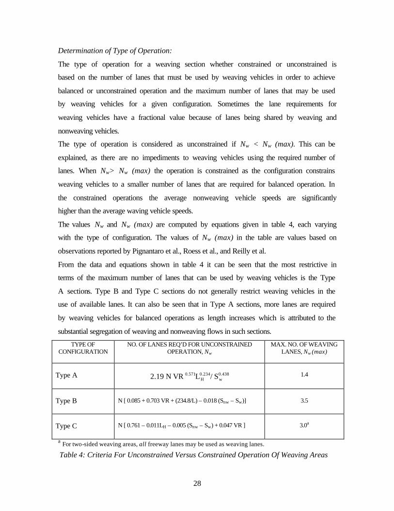
Determination of Type of Operation:
The type of operation for a weaving section whether constrained or unconstrained is
based on the number of lanes that must be used by weaving vehicles in order to achieve
balanced or unconstrained operation and the maximum number of lanes that may be used
by weaving vehicles for a given configuration. Sometimes the lane requirements for
weaving vehicles have a fractional value because of lanes being shared by weaving and
nonweaving vehicles.
The type of operation is considered as unconstrained if Nw < Nw (max). This can be
explained, as there are no impediments to weaving vehicles using the required number of
lanes. When Nw> Nw (max) the operation is constrained as the configuration constrains
weaving vehicles to a smaller number of lanes that are required for balanced operation. In
the constrained operations the average nonweaving vehicle speeds are significantly
higher than the average waving vehicle speeds.
The values Nw and Nw (max) are computed by equations given in table 4, each varying
with the type of configuration. The values of Nw (max) in the table are values based on
observations reported by Pignantaro et al., Roess et al., and Reilly et al.
From the data and equations shown in table 4 it can be seen that the most restrictive in
terms of the maximum number of lanes that can be used by weaving vehicles is the Type
A sections. Type B and Type C sections do not generally restrict weaving vehicles in the
use of available lanes. It can also be seen that in Type A sections, more lanes are required
by weaving vehicles for balanced operations as length increases which is attributed to the
substantial segregation of weaving and nonweaving flows in such sections.
TYPE OF CONFIGURATION
NO. OF LANES REQ’D FOR UNCONSTRAINED OPERATION, Nw
MAX. NO. OF WEAVING LANES, Nw (max)
Type A
0.438w
0.234H
0.571 S/ LVRN 19.2
1.4
Type B
N [ 0.085 + 0.703 VR + (234.8/L) – 0.018 (Snw – Sw)]
3.5
Type C
N [ 0.761 – 0.011LH – 0.005 (Snw – Sw) + 0.047 VR ]
3.0a
a For two-sided weaving areas, all freeway lanes may be used as weaving lanes.
Table 4: Criteria For Unconstrained Versus Constrained Operation Of Weaving Areas
29
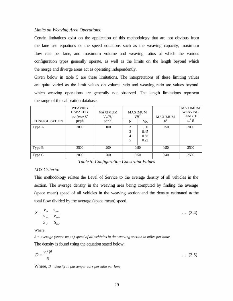
Limits on Weaving Area Operations:
Certain limitations exist on the application of this methodology that are not obvious from
the lane use equations or the speed equations such as the weaving capacity, maximum
flow rate per lane, and maximum volume and weaving ratios at which the various
configuration types generally operate, as well as the limits on the length beyond which
the merge and diverge areas act as operating independently.
Given below in table 5 are these limitations. The interpretations of these limiting values
are quire varied as the limit values on volume ratio and weaving ratio are values beyond
which weaving operations are generally not observed. The length limitations represent
the range of the calibration database.
MAXIMUM
VRC
CONFIGURATION
WEAVING CAPACITY vW (max),a
pcph
MAXIMUM
Vv/N,b pcphl N VR
MAXIMUM Rd
MAXIMUM WEAVING LENGTH
L,e ft
Type A
2000
100
2 3 4 5
1.00 0.45 0.35 0.22
0.50
2000
Type B 3500 200 0.80 0.50 2500
Type C 3000 200 0.50 0.40 2500
Table 5: Configuration Constraint Values
LOS Criteria:
This methodology relates the Level of Service to the average density of all vehicles in the
section. The average density in the weaving area being computed by finding the average
(space mean) speed of all vehicles in the weaving section and the density estimated as the
total flow divided by the average (space mean) speed.
nw
nw
w
w
nww
Sv
Sv
vvS
+
+= …..(3.4)
Where,
S = average (space mean) speed of all vehicles in the weaving section in miles per hour.
The density is found using the equation stated below:
SNv
D/
= …..(3.5)
Where, D= density in passenger cars per mile per lane.
30
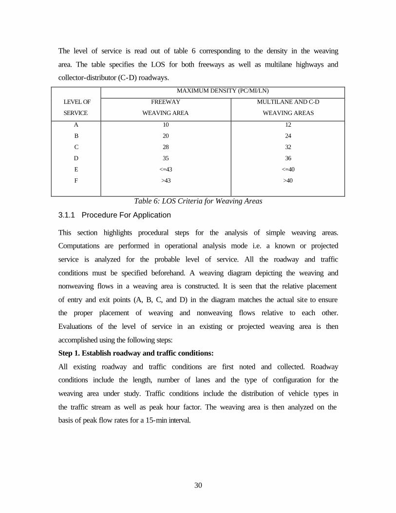
The level of service is read out of table 6 corresponding to the density in the weaving
area. The table specifies the LOS for both freeways as well as multilane highways and
collector-distributor (C-D) roadways.
MAXIMUM DENSITY (PC/MI/LN)
LEVEL OF
SERVICE
FREEWAY
WEAVING AREA
MULTILANE AND C-D
WEAVING AREAS
A
B
C
D
E
F
10
20
28
35
<=43
>43
12
24
32
36
<=40
>40
Table 6: LOS Criteria for Weaving Areas
3.1.1 Procedure For Application This section highlights procedural steps for the analysis of simple weaving areas.
Computations are performed in operational analysis mode i.e. a known or projected
service is analyzed for the probable level of service. All the roadway and traffic
conditions must be specified beforehand. A weaving diagram depicting the weaving and
nonweaving flows in a weaving area is constructed. It is seen that the relative placement
of entry and exit points (A, B, C, and D) in the diagram matches the actual site to ensure
the proper placement of weaving and nonweaving flows relative to each other.
Evaluations of the level of service in an existing or projected weaving area is then
accomplished using the following steps:
Step 1. Establish roadway and traffic conditions:
All existing roadway and traffic conditions are first noted and collected. Roadway
conditions include the length, number of lanes and the type of configuration for the
weaving area under study. Traffic conditions include the distribution of vehicle types in
the traffic stream as well as peak hour factor. The weaving area is then analyzed on the
basis of peak flow rates for a 15-min interval.

31
Step 2. Convert all traffic volumes to peak flow rates
As the speed and lane use algorithms are based on peak flow rates, all component flows
must be converted to flow rate for peak 15 min, by using following equation:
pwHV xfxfPHFxfV
v = …..(3.6)
Where, v=flow rate for peak 15 min under ideal conditions (pcph);
V=hourly volume under prevailing conditions (veh/hr);
PHF= peak-hour Factor;
fHV=heavy-vehicle adjustment factor;
fp=driver population adjustment factor.
Step 3. Construction of Weaving Diagram
It is necessary and helpful to construct a weaving diagram that shows all flows indicated
at peak flow rates under ideal conditions in passenger cars per hour.
Step 4. Computation of Unconstrained Weaving and Nonweaving Speeds
In this step it is assumed that the operation is unconstrained. The weaving intensity factor
for the appropriate configuration is read from table 3. The average (space mean) speed is
then computed for the weaving and nonweaving vehicles.
Step 5. Check for Constrained operation
Using the speeds computed in the previous step, an estimate of the number of lanes used
by weaving vehicles to achieve unconstrained operation is made using the equations
specified in the table 4. This computed value of Nw is then compared with Nw (max) (read
from table 4).
If Nw (max) is less than or equal to Nw then the operation is constrained as per definition
and hence the assumption that this is an unconstrained operation is accurate. If the
condition is not satisfied then the operation is constrained and the values of the weaving
and nonweaving speeds are recomputed using the constrained weaving intensity factor
for the appropriate configuration.
Step 6. Computation of Average (Space Mean) Speed and Density in Weaving Area
The equation stated earlier in the methodology is used to compute the average (space
mean) speed of all vehicles in the weaving section. Then this average speed (space mean)
is used in the equation to compute the density of the weaving area.
32
Step 7. Check for Weaving Area Limitations
As a final check to see if the whole analysis is acceptable the table specifying the
limitations on the weaving sections is consulted and is made sure that none of the
parameters have exceeded their limits specified by the table.
Step 8. Determination of Level of Service
The estimated value of density, D, in the weaving area is compared with the criteria in the
table 6 to determine the prevailing Level of Service.
3.2 TRANSIMS Methodology
TRANSIMS consists of mutually supporting simulations, models, and databases that
employ advanced computational and analytical techniques to create an integrated regional
transportation system analysis environment. By applying advanced technologies and
methods, it simulates the dynamic details that contribute to the complexity inherent in
transportation issues. The integrated results from the detailed simulations help address
environmental pollution, energy consumption, traffic congestion, land use planning,
traffic safety, intelligent vehicle efficiencies, and the transportation infrastructure effect
on the quality of life, productivity, and economy. (TRANSIMS website)
TRANSIMS is a five-module software package; each module dealing with a specific
task. The modules are Population Synthesizer, Activity Generator, Route Planner,
Microsimulator and a Selector. Another module is the Emissions Estimator, which as the
name suggests calculates the amount of emissions for the region in analysis using the
outputs of the above-mentioned previous five modules. An interaction among the
modules is depicted in Figure 4.
A very brief description of what each module does is presented next starting with the
Population Synthesizer. This module of TRANSIMS uses the PUMS data and the STF-
3A data provided by the Census to create synthetic population having the same aggregate
characteristics to those in the census data. This module also locates this synthetic
population on transportation network using a suitable algorithm.
The Activity Generator then assigns activities to these synthetic population based on the
activity survey data depending on the household and demographic characteristics using
the CART algorithm. Once the synthetic population is in place with their respective

33
activities the Route Planner designates to each traveler his travel plans, i.e., how he/she
goes about doing his/her activities. Should the activity of synthetic household include
activities that require travel on the transportation network, the Route Planner finds the
shortest path using various shortest path algorithms and assigns the traveler his exact
itinerary detailing the links and nodes he travels on to reach his destination.
On having these plans and the transportation network, the Microsimulator simulates the
plans for all travelers on the network, their movements being governed by some simple
rules. The Microsimulator uses a cellular automata approach for simulating vehicles on
the network. Traffic behavior that the analyst wants to study is collected as the simulation
progresses.
The selector module provides the feedback for the whole process so that any unrealistic
data such as an infeasible plan or an unlocatable household can be dealt by redoing his
plan or relocating him with changed household characteristics or demographics.
As this research mainly deals with analyzing weaving areas, it is noted that the
Microsimulator is the only module that affects it. For this reason the following section
discusses in detail about its working, logic and rationale for vehicle movements.
3.2.1 Microsimulator Introduction
The TRANSIMS Microsimulator module simulates the movement and the interactions of
travelers in the transportation system of the study area. In this module every traveler tries
to execute his/her travel movements according to plan. These movements and interactions
produce key data that is output from the Microsimulator, bringing about more
macroscopic quantities like volume, flow etc by aggregation of these individual
interactions. The Microsimulator imitates realistic traffic behavior in decisions about lane
changes, passing slow vehicles and evaluating interactions with other vehicles.
A coarse simulation approach entitled “Cellular Automata” (CA) is used to keep up with
a fast computational speed necessary to simulate very large region. TRANSIMS
Microsimulator also provides the capability of using multiple CPUs to support a large
number of travelers and a considerable size transportation network.
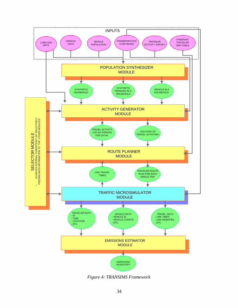
34
Figure 4: TRANSIMS Framework
INPUTS
POPULATION SYNTHESIZERMODULE
CENSUS DATA
LAND-USEDATA
TRANSPORTATION NETWORK
VEHICLEPOPULATION
ITINERANTTRAVELERTRIP-TABLE
TRAVELERACTIVITY SURVEY
SE
LEC
TO
R M
OD
ULE
�A
CH
IEV
ES
INT
ER
NA
L C
ON
SIS
TE
NC
Y B
Y S
ELE
CT
IVE
LYF
EE
DIN
G B
AC
K IN
FO
RM
AT
ION
TO
TH
E O
TH
ER
MO
DU
LES
SYNTHETICHOUSEHOLD
VEHICLE IN AHOUSEHOLD
SYNTHETICPERSONS IN AHOUSEHOLD
TRAVEL ACTIVITYLIST BY PERSON
FOR 24 Hrs.
ACTIVITY GENERATORMODULE
ROUTE PLANNERMODULE
TRAFFIC MICROSIMULATORMODULE
EMISSIONS ESTIMATORMODULE
LOCATION OFTRAVEL ACTIVITIES
LINK TRAVELTIMES
TRAVELER ROUTEPLAN FOR EACH
SINGLE TRIP
TRAVELER DATA - ID - TIME - LOCATION - ETC.
TRAVEL DATA - LINK TIMES - LINK DENSITIES - ETC.
VEHICLE DATA - VEHICLE ID - VEHICLE COUNTS - ETC.
EMISSIONSINVENTORY

35
The Cellular Automata approach divides every link on the network into a finite number
of cells. At every timestep each of these “cells” is scanned for a vehicle presence. If a
vehicle is present, the vehicle position is advanced to another cell using a simple rule set.
Reducing the size of the “cell”, expanding the rule set and adding vehicle attributes
increases the fidelity of the Microsimulator but would greatly affect the computational
speed. The size of 7.5 meters length and a traffic lane in width is chosen as a default
value for the “cell” for TRANSIMS.
The input to the Microsimulator aside from the traveler’s plans includes data about the
transportation network, vehicles, transit and traveler plans. The outputs from the
Microsimulator include spatial, temporal summary data (e.g., densities, travel times etc.),
snapshot data and traveler event data as shown in Figure 5.
A brief explanation of the Microsimulator is also presented in Figure 5 and is explained
in detail in the following sections.
Figure 5: Overview Of Microsimulator
Perform Vehicle Movement
Vehicles Enter Parking
Migrate Vehicles
Vehicles Leave Intersections
Vehicles Enter Intersections
Collect Output Partition Network
Queue Vehicles on parking places
Place Travelers on Network
Update Signals
Perform Lane Changes
Vehicles Exit Parking
Network Data
Vehicles
Transit Data
Traveler Plans
Traveler Event Data
Snapshot Data
Summary Data
MICROSIMULATOR FUNCTIONS
INPUT OUTPUT
Nex
t T
imes
tep
Servicing Transit Stop

36
3.2.2 Input Data
Figure 6: Major Inputs To The Microsimulator
This section highlights the various inputs to the Microsimulator. These inputs can be
grouped into four different categories, each providing information critical to the operation
of the Microsimulator.
The inputs to the Microsimulator include the Network Data files, the Vehicle files, the
Transit Data files and the Traveler Plans. These data files provide sufficient information
for the Microsimulator to simulate the movements and the interactions of the travelers in
the transportation study area. The detail of the information input also influences the
coarseness of the Microsimulator output. Some studies may require highly detailed
information about the network while some others may require just the minimum to
construct a network.
Network Data • Nodes • Links • Lane Use And Connectivity • Intersections (signals & signs) • Activity Locations • Parking
2. Vehicles
Transit Data • Route Paths in Network • Schedule of Stops • Driver Plans • Vehicle Properties
4. Major Inputs
Network Data
• Nodes • Links • Lane Use And Connectivity • Intersections (signals & signs) • Activity Locations • Parking • Transit Stops
Vehicles
Transit Data • Route Paths in Network • Schedule of Stops • Driver Plans • Vehicle Properties (e.g. Starting
Location)
Traveler Plans
Microsimulator
1. Major Inputs
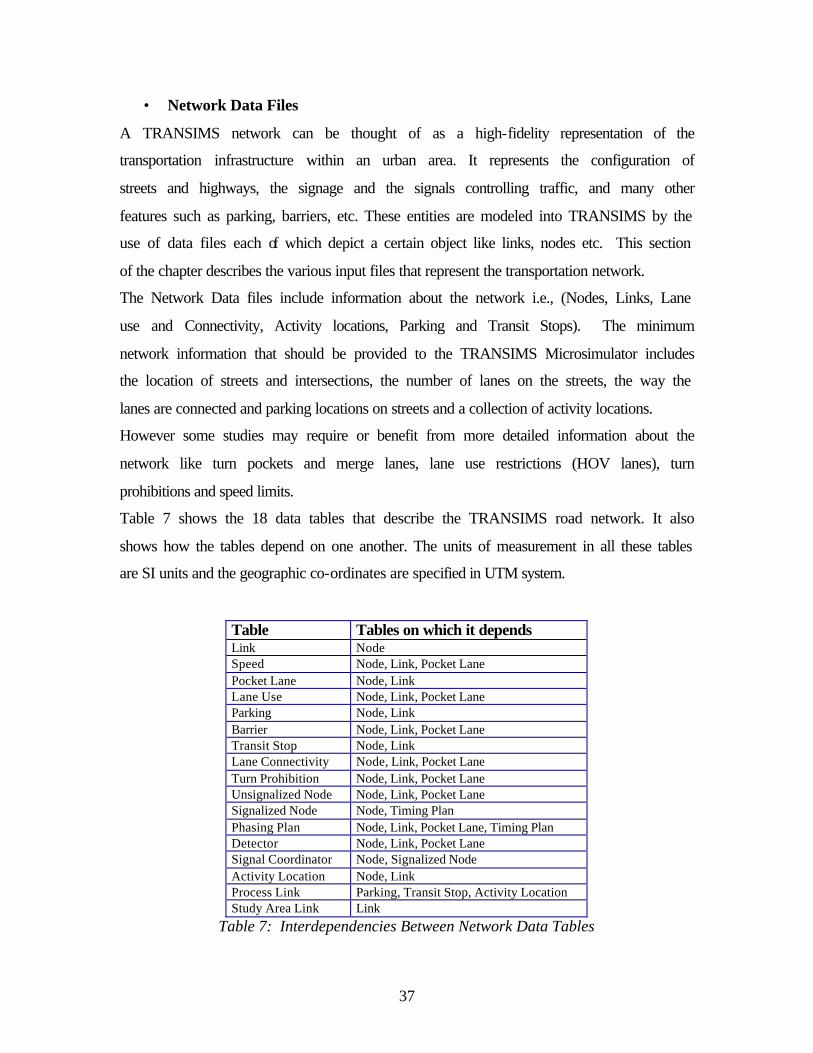
37
• Network Data Files
A TRANSIMS network can be thought of as a high-fidelity representation of the
transportation infrastructure within an urban area. It represents the configuration of
streets and highways, the signage and the signals controlling traffic, and many other
features such as parking, barriers, etc. These entities are modeled into TRANSIMS by the
use of data files each of which depict a certain object like links, nodes etc. This section
of the chapter describes the various input files that represent the transportation network.
The Network Data files include information about the network i.e., (Nodes, Links, Lane
use and Connectivity, Activity locations, Parking and Transit Stops). The minimum
network information that should be provided to the TRANSIMS Microsimulator includes
the location of streets and intersections, the number of lanes on the streets, the way the
lanes are connected and parking locations on streets and a collection of activity locations.
However some studies may require or benefit from more detailed information about the
network like turn pockets and merge lanes, lane use restrictions (HOV lanes), turn
prohibitions and speed limits.
Table 7 shows the 18 data tables that describe the TRANSIMS road network. It also
shows how the tables depend on one another. The units of measurement in all these tables
are SI units and the geographic co-ordinates are specified in UTM system.
Table Tables on which it depends Link Node Speed Node, Link, Pocket Lane Pocket Lane Node, Link Lane Use Node, Link, Pocket Lane Parking Node, Link Barrier Node, Link, Pocket Lane Transit Stop Node, Link Lane Connectivity Node, Link, Pocket Lane Turn Prohibition Node, Link, Pocket Lane Unsignalized Node Node, Link, Pocket Lane Signalized Node Node, Timing Plan Phasing Plan Node, Link, Pocket Lane, Timing Plan Detector Node, Link, Pocket Lane Signal Coordinator Node, Signalized Node Activity Location Node, Link Process Link Parking, Transit Stop, Activity Location Study Area Link Link
Table 7: Interdependencies Between Network Data Tables
38
• Vehicle Data files
The Microsimulator also reads in the vehicle data files, which affects vehicle usage (e.g.,
transit, private auto, taxi etc.) referred to as vehicle specification file and vehicle
characteristics (length, acceleration, profile, etc.) referred to as the vehicle prototype file.
The TRANSIMS Population Synthesizer generates and assigns private vehicles to
households and the Activity Generator assigns a possible set of vehicles to each member
of a household. Freight and transit vehicles, though generated by separate utilities, are
included in the vehicle database. Every freight and transit vehicle has a unique ID.
• Transit Data Files
The Transit Data required by the TRANSIMS Microsimulator deals with the route paths
of transit vehicles in the network, the schedule of stops, the transit drivers plans, and the
vehicle properties each specified to TRANSIMS through a separate file such as the
Transit route file, Transit schedule file.
• Traveler Plans
The other input to the Microsimulator are the travelers’ plans that are typically generated
by the Route Planner. The Microsimulator executes these plans for individual travelers
and the interactions of which on the transportation network provide the traffic patterns
and behavior.
3.2.3 TRANSIMS Microsimulator Logic
This section highlights how the Microsimulator conducts the movements of the travelers
encompassing vehicle movements, lane changes, traversal across intersections, transit
scheduling, entry and exit from parking places etc.
At the beginning of the simulation, the Microsimulator reads in the transportation
network files followed location of every vehicle on the network and the traveler’s plans.
The travelers are then placed on the network and allowed to move from their origins to
their destinations. For non-simulated modes, such as movement from a transit stop to a
parking place- a traveler is removed from the buffer in one activity (transit stop) and
placed in the buffer on another activity (parking place), with a new departure time
reflecting the estimated duration of the trip in the process link. Vehicles (simulated mode)
are moved from one grid cell to another using the rules embedded in the CA approach, to
be described next, with modifications to support lane changing and plan following until
39
they reach the end of the grid. There they wait for an acceptable gap in the traffic or for
protection at a signal before moving through the intersection onto the next grid. This
continues until each vehicle reaches its destination, where it is removed from the grid.
In carrying out the movements of travelers and vehicles on the transportation network,
the Microsimulator invokes several procedures categorized as follows:
• Placing Travelers and Vehicles on the Network,
• Updating the location of each Traveler and Vehicle,
• Preparing for a Timestep,
• Cleaning up after a Timestep, and
• Supporting Parallel Computation.
The following sections address these five procedures.
Placing Travelers and Vehicles On Network
The placement of the travelers and the vehicles on the network takes place at the start of
the simulation. In this initialization step, all the input information required to run the
Microsimulator is read from the vehicle, the plan, the transit route, and the network files.
The vehicle and the plan files are accessed through an index, which are generated from an
appropriate file. A list of Vehicle IDs located at each parking accessory is initialized from
the vehicles file.
The Microsimulator reads in the traveler plans (i.e., legs of a plan) using the index sorted
by expected departure time, until all the plans departing before or on the current
simulation time are read. In addition, the ID’s of the hibernating travelers (those who
have already executed one leg of their plan and are waiting to depart on another) are
popped off the queue of Arrived Traveler list. The next leg of plan for each of the arrived
travelers is read using an index that is sorted according to the traveler ID.
For a traveler to get onto the transportation network, the corresponding plan needs to be:
a) local; originating in an accessory (transit stop or parking place) that is a part of the
network under the control of the CPU and b) should be active (expected arrival time
before the simulation start time and departure time before the simulation end time). The
transportation network is partitioned into several CPUs to facilitate the running of the
simulation.
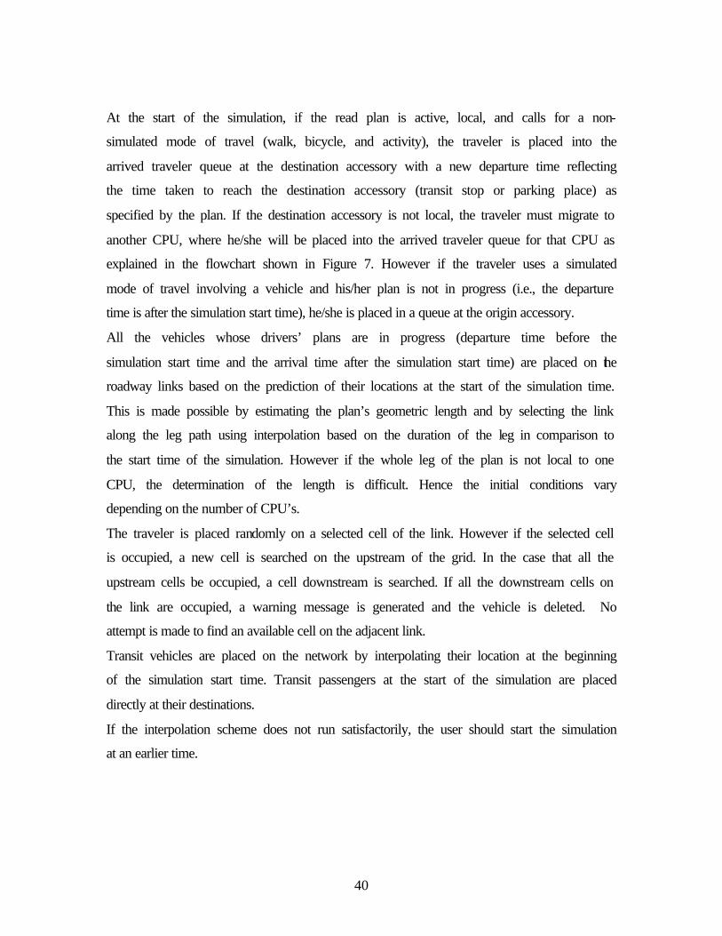
40
At the start of the simulation, if the read plan is active, local, and calls for a non-
simulated mode of travel (walk, bicycle, and activity), the traveler is placed into the
arrived traveler queue at the destination accessory with a new departure time reflecting
the time taken to reach the destination accessory (transit stop or parking place) as
specified by the plan. If the destination accessory is not local, the traveler must migrate to
another CPU, where he/she will be placed into the arrived traveler queue for that CPU as
explained in the flowchart shown in Figure 7. However if the traveler uses a simulated
mode of travel involving a vehicle and his/her plan is not in progress (i.e., the departure
time is after the simulation start time), he/she is placed in a queue at the origin accessory.
All the vehicles whose drivers’ plans are in progress (departure time before the
simulation start time and the arrival time after the simulation start time) are placed on the
roadway links based on the prediction of their locations at the start of the simulation time.
This is made possible by estimating the plan’s geometric length and by selecting the link
along the leg path using interpolation based on the duration of the leg in comparison to
the start time of the simulation. However if the whole leg of the plan is not local to one
CPU, the determination of the length is difficult. Hence the initial conditions vary
depending on the number of CPU’s.
The traveler is placed randomly on a selected cell of the link. However if the selected cell
is occupied, a new cell is searched on the upstream of the grid. In the case that all the
upstream cells be occupied, a cell downstream is searched. If all the downstream cells on
the link are occupied, a warning message is generated and the vehicle is deleted. No
attempt is made to find an available cell on the adjacent link.
Transit vehicles are placed on the network by interpolating their location at the beginning
of the simulation start time. Transit passengers at the start of the simulation are placed
directly at their destinations.
If the interpolation scheme does not run satisfactorily, the user should start the simulation
at an earlier time.
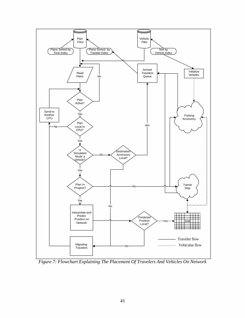
41
Plan Files
Vehicle Files
ReadPlans
PlanActive?
isSimulatedMode aVehicle?
Plan InProgres?
PredictedPositionLocal?
ParkingAccessory
TransitStop
Grid
Yes
Yes
Yes
No
Yes
DestinationAccessory
Local?
yes
No
No
No
No
Plans Sorted byTraveler Index
Plans Sorted byTime Index
Sort byVehicle Index
InitializeVehicles
PlanLocal toCPU?
Yes
No
Send toAnother
CPU
Interpolate andPredict
Position onNetwork
ArrivedTravelersQueue
MigratingTravelers
Figure 7: Flowchart Explaining The Placement Of Travelers And Vehicles On Network
Traveler flow
Vehicular flow
42
Update Travelers Locations
After reading and placing travelers, the simulation executes their plans one step at a time.
A single timestep is broken down into several events as shown in Figure 8.
Figure 8: Microsimulator Steps In Each Timestep Update
To accomplish a simulation update of the vehicle movements involved in carrying out
each traveler plan, the following steps are executed:
a) Perform lane changes for passing and lane following
b) Service Transit stop
c) Exit vehicles from parking places
d) Move vehicles in the same lane
e) Enter vehicles to parking places
f) Perform movements at Intersections: divided into
i) Unsignalized Intersections
ii) Signalized Intersections
g) Mark vehicles off-plan
Perform Vehicle Movement
Vehicles Enter Parking Places
Migrate Vehicles
Vehicles Leave Intersections
Vehicles Enter Intersections
Collect Output Partition Network
Queue Vehicles on parking places
Place Travelers on Network
Update Signals
Perform Lane Changes
Vehicles Exit Parking
Nex
t T
imes
tep
Initialization Step
Service Transit Stop
43
Although the sequence for the timestep update of vehicle movements is as stated above,
the presentation of the material is given in a slightly different sequence in order to
facilitate the understanding of the material by the reader.
• General Movement In The Same Lane
Vehicles in the TRANSIMS network follow simple rules that govern their movements.
These rules are intentionally kept simple to enhance the computation speed considering
the millions of interactions taking place in the system. At the core, the rules for a vehicle
movement in the same lane could be put simply as “Acceleration whenever possible,
Deceleration only if necessary and sometimes for no reason”.
The decision by a vehicle to accelerate or decelerate depends on its current speed, and the
gap between it and the immediate vehicle ahead in the same lane. Another factor that
influences the movement of a vehicle is the deceleration probability (Pd), which can be
thought of as the probability of a vehicle decelerating in the timestep. All the vehicles in
the TRANSIMS network are constrained by a maximum attainable speed that is specified
(VGlobalMax, which is 5 cells/timestep or about 80 mph).
Consider a vehicle traveling at a certain speed at a given timestep. Now if the vehicle
speed is greater than the gap ahead, the vehicle needs to reduce its speed to avoid a
collision. The amount of deceleration being subject to, depends on how large or small the
current gap (Gc) is compared to the current speed. To model aggressive breaking an
element of randomness in the form of Pd is used. If the probability of decelerating is
greater than a certain threshold value (Pnoise), the speed of the vehicle is further reduced
than what can be actually attainable based on gap (Gc).
Considering the scenario where the gap ahead of the vehicle is larger than its current
speed, then the vehicle can possibly accelerate. The magnitude of acceleration is
specified differently for each type of vehicle. For autos, the maximum acceleration At, is
specified in the vehicle prototype file. For trucks and other vehicles, the grade of the road
plays an important role in determining the magnitude of acceleration. All velocity and
acceleration changes are integer values based on the number of cells/second or
cells/second/second respectively. In case calculated At is fractional then it is randomly
increased to a full number (60% of the time) and decreased to a full number (40% of the
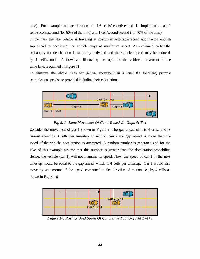
44
time). For example an acceleration of 1.6 cells/second/second is implemented as 2
cells/second/second (for 60% of the time) and 1 cell/second/second (for 40% of the time).
In the case that the vehicle is traveling at maximum allowable speed and having enough
gap ahead to accelerate, the vehicle stays at maximum speed. As explained earlier the
probability for deceleration is randomly activated and the vehicles speed may be reduced
by 1 cell/second. A flowchart, illustrating the logic for the vehicles movement in the
same lane, is outlined in Figure 11.
To illustrate the above rules for general movement in a lane, the following pictorial
examples on speeds are provided including their calculations.
Fig 9: In-Lane Movement Of Car 1 Based On Gaps At T=t
Consider the movement of car 1 shown in Figure 9. The gap ahead of it is 4 cells, and its
current speed is 3 cells per timestep or second. Since the gap ahead is more than the
speed of the vehicle, acceleration is attempted. A random number is generated and for the
sake of this example assume that this number is greater than the deceleration probability.
Hence, the vehicle (car 1) will not maintain its speed. Now, the speed of car 1 in the next
timestep would be equal to the gap ahead, which is 4 cells per timestep. Car 1 would also
move by an amount of the speed computed in the direction of motion i.e., by 4 cells as
shown in Figure 10.
Figure 10: Position And Speed Of Car 1 Based On Gaps At T=t+1
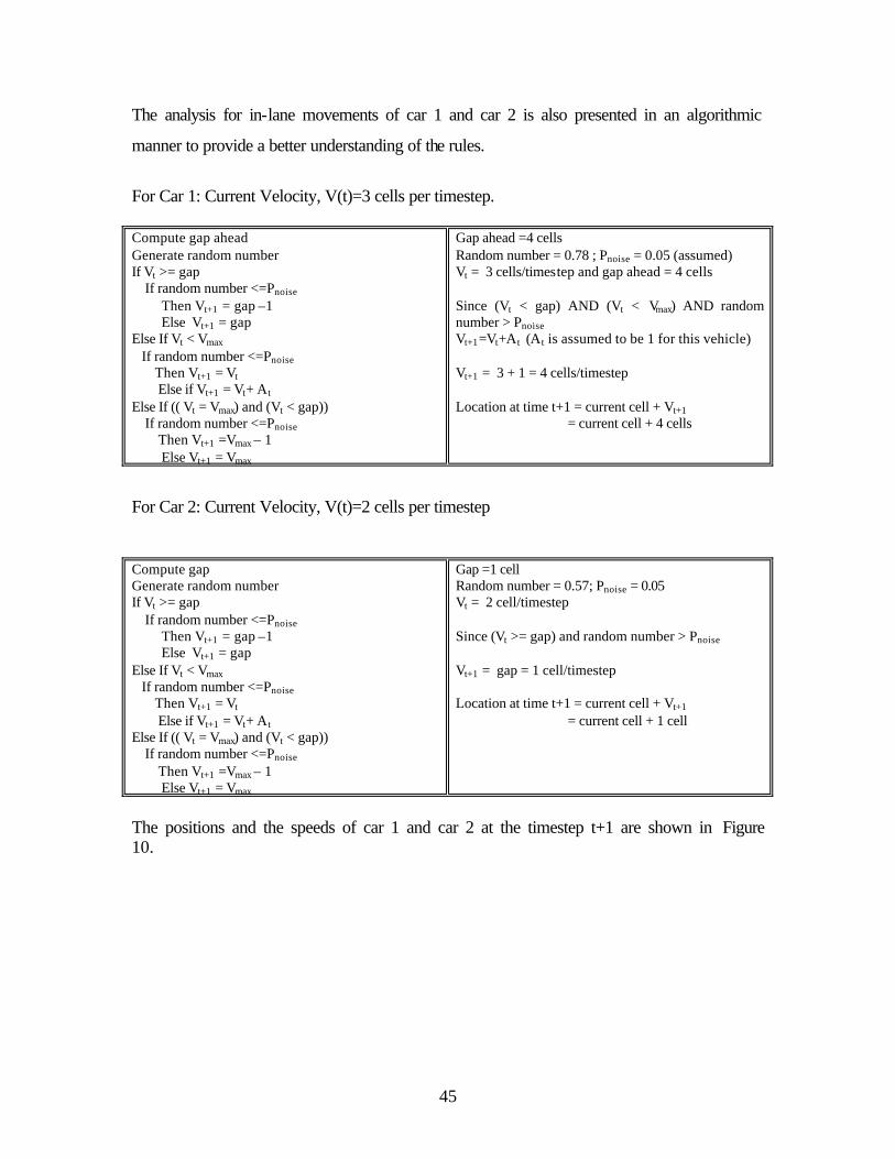
45
The analysis for in-lane movements of car 1 and car 2 is also presented in an algorithmic
manner to provide a better understanding of the rules.
For Car 1: Current Velocity, V(t)=3 cells per timestep. Compute gap ahead Generate random number If Vt >= gap If random number <=Pnoise Then Vt+1 = gap –1 Else Vt+1 = gap Else If Vt < Vmax If random number <=Pnoise Then Vt+1 = Vt Else if Vt+1 = Vt+ At Else If (( Vt = Vmax) and (Vt < gap)) If random number <=Pnoise Then Vt+1 =Vmax – 1 Else Vt+1 = Vmax
Gap ahead =4 cells Random number = 0.78 ; Pnoise = 0.05 (assumed) Vt = 3 cells/timestep and gap ahead = 4 cells Since (Vt < gap) AND (Vt < Vmax) AND random number > Pnoise Vt+1=Vt+At (At is assumed to be 1 for this vehicle) Vt+1 = 3 + 1 = 4 cells/timestep Location at time t+1 = current cell + Vt+1 = current cell + 4 cells
For Car 2: Current Velocity, V(t)=2 cells per timestep
Compute gap Generate random number If Vt >= gap If random number <=Pnoise Then Vt+1 = gap –1 Else Vt+1 = gap Else If Vt < Vmax If random number <=Pnoise Then Vt+1 = Vt Else if Vt+1 = Vt+ At Else If (( Vt = Vmax) and (Vt < gap)) If random number <=Pnoise Then Vt+1 =Vmax – 1 Else Vt+1 = Vmax
Gap =1 cell Random number = 0.57; Pnoise = 0.05 Vt = 2 cell/timestep Since (Vt >= gap) and random number > Pnoise Vt+1 = gap = 1 cell/timestep Location at time t+1 = current cell + Vt+1 = current cell + 1 cell
The positions and the speeds of car 1 and car 2 at the timestep t+1 are shown in Figure 10.
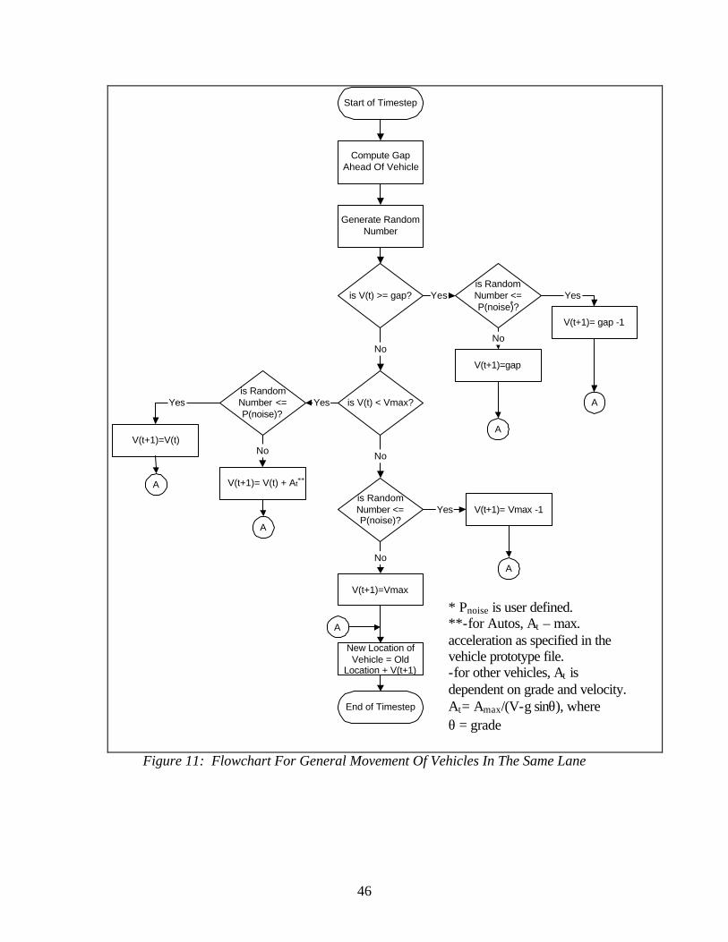
46
Start of Timestep
Compute GapAhead Of Vehicle
Generate RandomNumber
is V(t) >= gap?is RandomNumber <=P(noise)?
is V(t) < Vmax?is RandomNumber <=P(noise)?
is RandomNumber <=P(noise)?
V(t+1)= gap -1
V(t+1)=gap
V(t+1)= Vmax -1
V(t+1)=Vmax
V(t+1)=V(t)
V(t+1)= V(t) + At
Yes
Yes
Yes
Yes
Yes
NoNo
NoNo
No
A
A
A
A
A
End of Timestep
A
New Location ofVehicle = Old
Location + V(t+1)
Figure 11: Flowchart For General Movement Of Vehicles In The Same Lane
* Pnoise is user defined. **-for Autos, At – max. acceleration as specified in the vehicle prototype file. -for other vehicles, At is dependent on grade and velocity. At= Amax/(V-g sinθ), where θ = grade
*
**
47
• Performing Lane Changes
The lane-changing maneuver of a vehicle in TRANSIMS Microsimulator occurs to pass a
slower vehicle immediately ahead or to make turns at intersections following its current
plan. The decisions for lane changes take place before the in-lane movement of the
vehicles on the links occur. This ensures that the in-lane movement of the vehicles takes
into account the effect of lane changes.
Lane changes into the left lane and into the right lane are treated by the Microsimulator
on alternating timesteps. The left lane changes are made on even timesteps while the right
ones are made on odd timesteps. Multilane roadways are processed from left to the right
during left lane changing and from the right to the left during right lane changing
procedures. It should be noted that these lane change procedures are only explored if the
cell on the adjacent lane in which the vehicle is trying to change into is vacant.
The above mentioned lane changing procedures are discussed in detail below under two
separate categories. One category is for lane changing based purely on passing a slower
vehicle, and the other one is based on making turns at intersections to follow plan.
Lane changes based on passing slower vehicles:
The lane changes based on this criterion occur only if the speed of the vehicle under
consideration is more than or equal to the gap ahead of it in the current lane (Gc). Another
important consideration is the magnitude of the gaps in the adjacent lane to which the
vehicle is attempting a lane change into. The gap ahead of the vehicle in the new adjacent
lane (Gf) should be larger than the one in the current lane (Gc). The vehicle, before
making the necessary lane change, should also consider if the vehicle behind it in the new
lane is sufficiently far away (Gb) to avoid any kind of collision.
The above ideas are captured into the TRANSIMS Microsimulator using three variables
Weight1, Weight2 and Weight 3. The values of these weights are computed as shown in
Table 8. For a vehicle to make a lane change the following three criterions should be
satisfied: Weight1 be greater than zero; Weight1 be greater than Weight2, and Weigt1 be
greater than Weight 3.
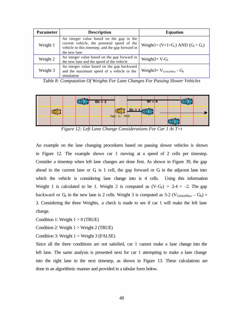
48
Parameter Description Equation
Weight 1 An integer value based on the gap in the current vehicle, the potential speed of the vehicle in this timestep, and the gap forward in the new lane
Weight1= (V+1>Gc) AND (Gf > Gc)
Weight 2 An integer value based on the gap forward in the new lane and the speed of the vehicle
Weight2= V-Gf
Weight 3 An integer value based on the gap backward and the maximum speed of a vehicle in the simulation
Weight3= VGlobalMax - Gb
Table 8: Computation Of Weights For Lane Changes For Passing Slower Vehicles
Figure 12: Left Lane Change Considerations For Car 1 At T=t
An example on the lane changing procedures based on passing slower vehicles is shown
in Figure 12. The example shows car 1 moving at a speed of 2 cells per timestep.
Consider a timestep when left lane changes are done first. As shown in Figure 39, the gap
ahead in the current lane or Gc is 1 cell, the gap forward or Gf in the adjacent lane into
which the vehicle is considering lane change into is 4 cells. Using this information
Weight 1 is calculated to be 1. Weight 2 is computed as (V-Gf) = 2-4 = -2. The gap
backward or Gb in the new lane is 2 cells. Weight 3 is computed as 5-2 (VGlobalMax – Gb) =
3. Considering the three Weights, a check is made to see if car 1 will make the left lane
change.
Condition 1: Weight 1 > 0 (TRUE)
Condition 2: Weight 1 > Weight 2 (TRUE)
Condition 3: Weight 1 > Weight 3 (FALSE)
Since all the three conditions are not satisfied, car 1 cannot make a lane change into the
left lane. The same analysis is presented next for car 1 attempting to make a lane change
into the right lane in the next timestep, as shown in Figure 13. These calculations are
done in an algorithmic manner and provided in a tabular form below.
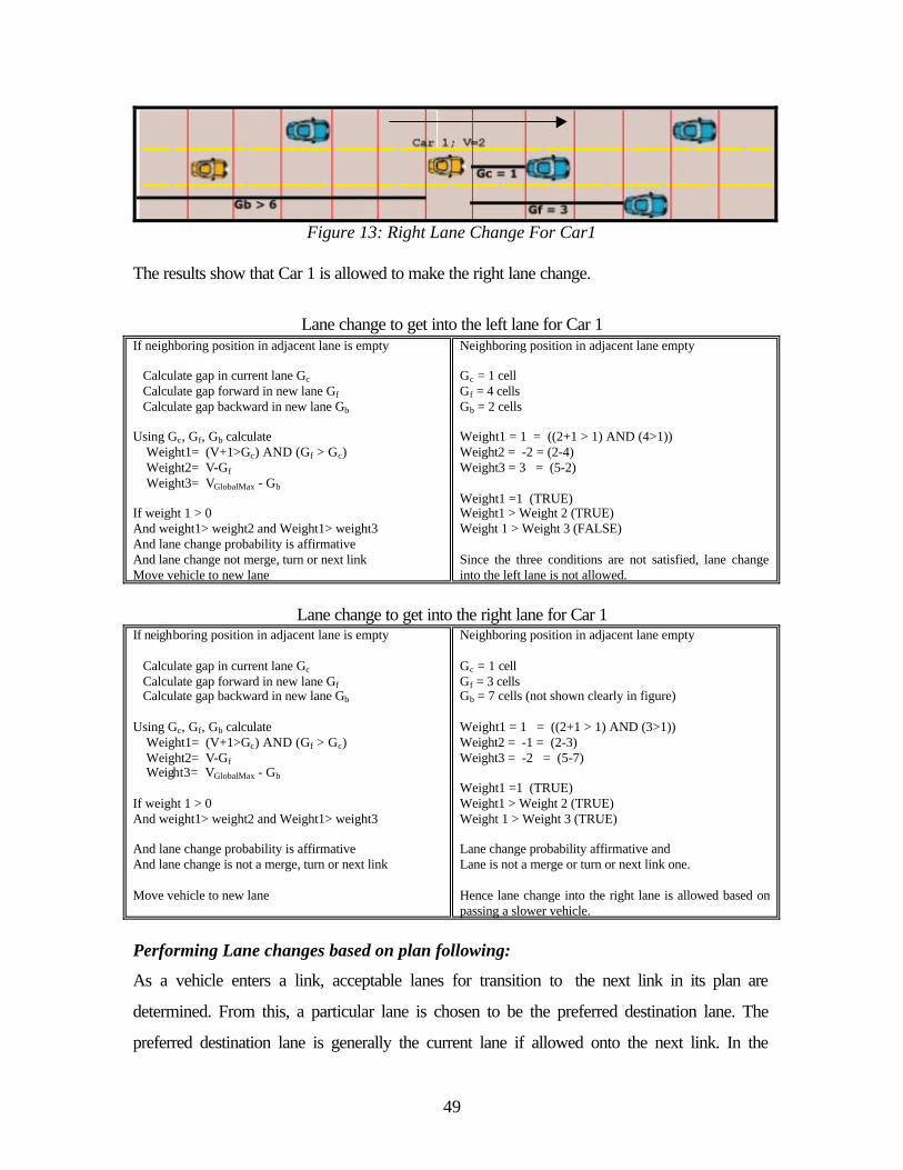
49
Figure 13: Right Lane Change For Car1
The results show that Car 1 is allowed to make the right lane change.
Lane change to get into the left lane for Car 1
If neighboring position in adjacent lane is empty Calculate gap in current lane Gc Calculate gap forward in new lane Gf Calculate gap backward in new lane Gb Using Gc, Gf, Gb calculate Weight1= (V+1>Gc) AND (Gf > Gc) Weight2= V-Gf Weight3= VGlobalMax - Gb If weight 1 > 0 And weight1> weight2 and Weight1> weight3 And lane change probability is affirmative And lane change not merge, turn or next link Move vehicle to new lane
Neighboring position in adjacent lane empty Gc = 1 cell Gf = 4 cells Gb = 2 cells Weight1 = 1 = ((2+1 > 1) AND (4>1)) Weight2 = -2 = (2-4) Weight3 = 3 = (5-2) Weight1 =1 (TRUE) Weight1 > Weight 2 (TRUE) Weight 1 > Weight 3 (FALSE) Since the three conditions are not satisfied, lane change into the left lane is not allowed.
Lane change to get into the right lane for Car 1
If neighboring position in adjacent lane is empty Calculate gap in current lane Gc Calculate gap forward in new lane Gf Calculate gap backward in new lane Gb Using Gc, Gf, Gb calculate Weight1= (V+1>Gc) AND (Gf > Gc) Weight2= V-Gf Weight3= VGlobalMax - Gb If weight 1 > 0 And weight1> weight2 and Weight1> weight3 And lane change probability is affirmative And lane change is not a merge, turn or next link Move vehicle to new lane
Neighboring position in adjacent lane empty Gc = 1 cell Gf = 3 cells Gb = 7 cells (not shown clearly in figure) Weight1 = 1 = ((2+1 > 1) AND (3>1)) Weight2 = -1 = (2-3) Weight3 = -2 = (5-7) Weight1 =1 (TRUE) Weight1 > Weight 2 (TRUE) Weight 1 > Weight 3 (TRUE) Lane change probability affirmative and Lane is not a merge or turn or next link one. Hence lane change into the right lane is allowed based on passing a slower vehicle.
Performing Lane changes based on plan following:
As a vehicle enters a link, acceptable lanes for transition to the next link in its plan are
determined. From this, a particular lane is chosen to be the preferred destination lane. The
preferred destination lane is generally the current lane if allowed onto the next link. In the
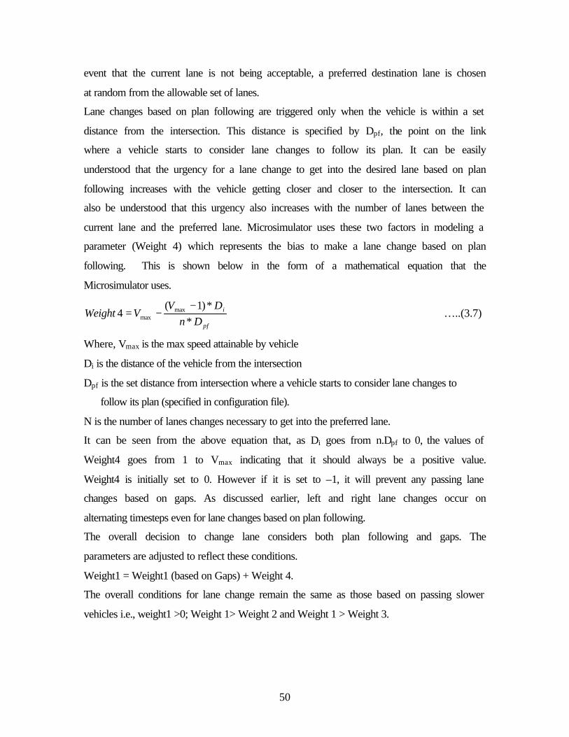
50
event that the current lane is not being acceptable, a preferred destination lane is chosen
at random from the allowable set of lanes.
Lane changes based on plan following are triggered only when the vehicle is within a set
distance from the intersection. This distance is specified by Dpf, the point on the link
where a vehicle starts to consider lane changes to follow its plan. It can be easily
understood that the urgency for a lane change to get into the desired lane based on plan
following increases with the vehicle getting closer and closer to the intersection. It can
also be understood that this urgency also increases with the number of lanes between the
current lane and the preferred lane. Microsimulator uses these two factors in modeling a
parameter (Weight 4) which represents the bias to make a lane change based on plan
following. This is shown below in the form of a mathematical equation that the
Microsimulator uses.
pf
i
DnDV
VWeight*
*)1(4 max
max
−−= …..(3.7)
Where, Vmax is the max speed attainable by vehicle
Di is the distance of the vehicle from the intersection
Dpf is the set distance from intersection where a vehicle starts to consider lane changes to
follow its plan (specified in configuration file).
N is the number of lanes changes necessary to get into the preferred lane.
It can be seen from the above equation that, as Di goes from n.Dpf to 0, the values of
Weight4 goes from 1 to Vmax indicating that it should always be a positive value.
Weight4 is initially set to 0. However if it is set to –1, it will prevent any passing lane
changes based on gaps. As discussed earlier, left and right lane changes occur on
alternating timesteps even for lane changes based on plan following.
The overall decision to change lane considers both plan following and gaps. The
parameters are adjusted to reflect these conditions.
Weight1 = Weight1 (based on Gaps) + Weight 4.
The overall conditions for lane change remain the same as those based on passing slower
vehicles i.e., weight1 >0; Weight 1> Weight 2 and Weight 1 > Weight 3.
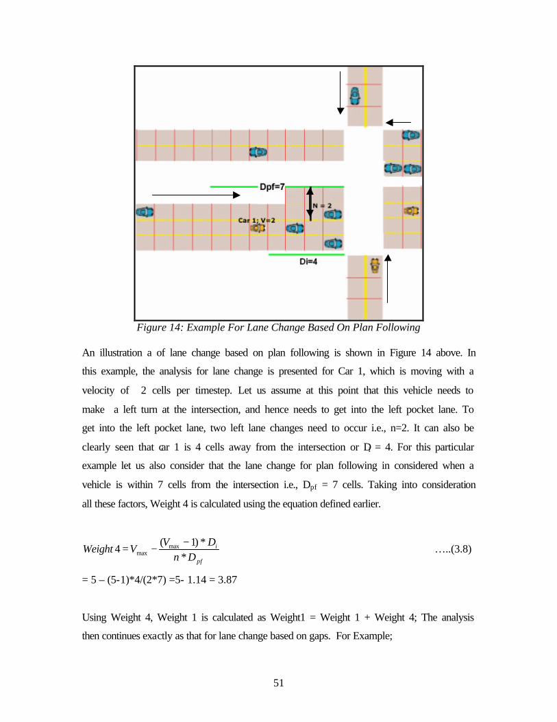
51
Figure 14: Example For Lane Change Based On Plan Following
An illustration a of lane change based on plan following is shown in Figure 14 above. In
this example, the analysis for lane change is presented for Car 1, which is moving with a
velocity of 2 cells per timestep. Let us assume at this point that this vehicle needs to
make a left turn at the intersection, and hence needs to get into the left pocket lane. To
get into the left pocket lane, two left lane changes need to occur i.e., n=2. It can also be
clearly seen that car 1 is 4 cells away from the intersection or Di = 4. For this particular
example let us also consider that the lane change for plan following in considered when a
vehicle is within 7 cells from the intersection i.e., Dpf = 7 cells. Taking into consideration
all these factors, Weight 4 is calculated using the equation defined earlier.
pf
i
DnDV
VWeight*
*)1(4 max
max−
−= …..(3.8)
= 5 – (5-1)*4/(2*7) =5- 1.14 = 3.87
Using Weight 4, Weight 1 is calculated as Weight1 = Weight 1 + Weight 4; The analysis
then continues exactly as that for lane change based on gaps. For Example;
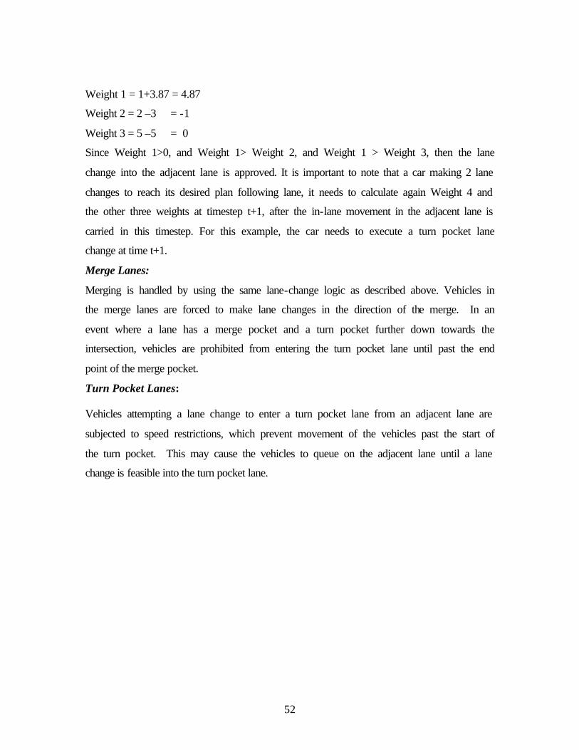
52
Weight 1 = 1+3.87 = 4.87
Weight 2 = 2 –3 = -1
Weight 3 = 5 –5 = 0
Since Weight 1>0, and Weight 1> Weight 2, and Weight 1 > Weight 3, then the lane
change into the adjacent lane is approved. It is important to note that a car making 2 lane
changes to reach its desired plan following lane, it needs to calculate again Weight 4 and
the other three weights at timestep t+1, after the in-lane movement in the adjacent lane is
carried in this timestep. For this example, the car needs to execute a turn pocket lane
change at time t+1.
Merge Lanes:
Merging is handled by using the same lane-change logic as described above. Vehicles in
the merge lanes are forced to make lane changes in the direction of the merge. In an
event where a lane has a merge pocket and a turn pocket further down towards the
intersection, vehicles are prohibited from entering the turn pocket lane until past the end
point of the merge pocket.
Turn Pocket Lanes: Vehicles attempting a lane change to enter a turn pocket lane from an adjacent lane are
subjected to speed restrictions, which prevent movement of the vehicles past the start of
the turn pocket. This may cause the vehicles to queue on the adjacent lane until a lane
change is feasible into the turn pocket lane.
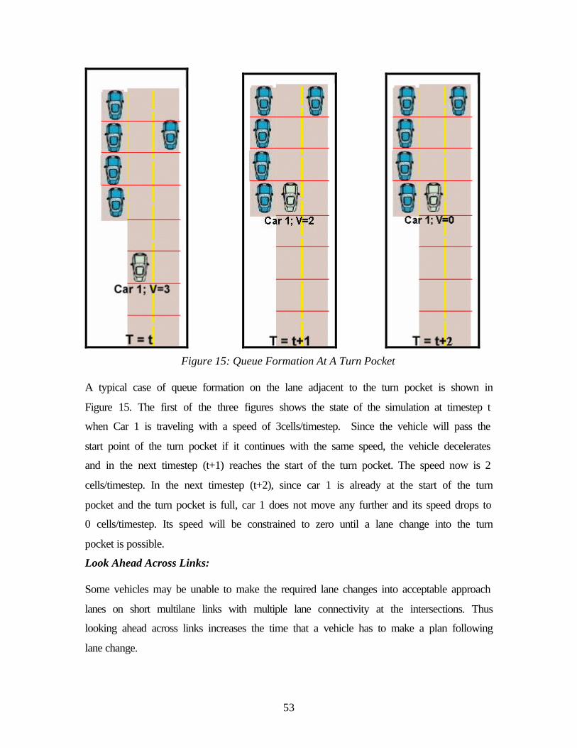
53
Figure 15: Queue Formation At A Turn Pocket
A typical case of queue formation on the lane adjacent to the turn pocket is shown in
Figure 15. The first of the three figures shows the state of the simulation at timestep t
when Car 1 is traveling with a speed of 3cells/timestep. Since the vehicle will pass the
start point of the turn pocket if it continues with the same speed, the vehicle decelerates
and in the next timestep (t+1) reaches the start of the turn pocket. The speed now is 2
cells/timestep. In the next timestep (t+2), since car 1 is already at the start of the turn
pocket and the turn pocket is full, car 1 does not move any further and its speed drops to
0 cells/timestep. Its speed will be constrained to zero until a lane change into the turn
pocket is possible.
Look Ahead Across Links: Some vehicles may be unable to make the required lane changes into acceptable approach
lanes on short multilane links with multiple lane connectivity at the intersections. Thus
looking ahead across links increases the time that a vehicle has to make a plan following
lane change.
54
The acceptable approach lanes are determined based on a plan look ahead distance. The
distance is used to determine how many links in the plan will be considered when
determining the approach lanes on the current link. A distance of 262.5 meters (35 grid
cells) is the default value. A value of 0.0 implies approach lanes are being determined by
considering the next link only.
A flowchart depicting the logic for all cases of lane changing in shown in Figure 16.
• Off-Plan Vehicles
Any vehicle becomes off-plan if it is not in the acceptable approach lane while entering a
link or an intersection and thus cannot follow its assigned plan. Also, vehicles attempting
to enter an intersection are marked off-plan if they have not moved for the duration of
time specified by the configuration key CA_MAX_WAITING_SECONDS. The number of
vehicles that become off-plan can be captured during the simulation output and are
referred to as lost vehicles.
TRANSIMS Microsimulator deals with the off-plan vehicles by keeping the vehicle in
simulation until a time again specified by the CA_OFF_PLAN_EXIT_TIME configuration
key is reached, after which the vehicle exits at the nearest parking location. In order to
keep the off-plan vehicle in simulation, new destination link is selected from the links
that are connected to the vehicles current lane. This method of choosing random links
occurs until the exit time for the vehicle is reached.
• Exit Travelers and Vehicles from Parking Places
A parking place accessory has a list of IDs for the vehicles that are present (either
because they begin the simulation there or they have arrived during the course of the
simulation). It also has a queue of travelers and their associated plans. This procedure
handles each traveler in the traveler queue whose departure time has arrived.
If the traveler is waiting for a vehicle, he or she cannot leave till the assigned vehicle with
appropriate ID is present. If the vehicle is not there, the traveler’s departure time is
incremented and he or she is replaced in the queue. A vehicle whose ID is on the list will
have been instantiated in the simulation only if it has arrived here from somewhere else.
Otherwise, a new vehicle with this ID must be created using the type implied by the
traveler’s plan.
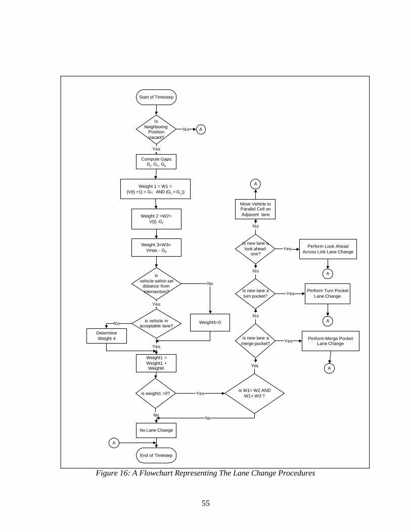
55
Start of Timestep
IsNeighboring
PositionVacant?
Compute GapsGc, G f, Gb
Weight 1 = W1 =(V(t) +1) > Gc AND (Gf > Gc))
Weight 2 =W2=V(t) -Gf
Weight 3=W3=Vmax - Gb
isvehicle within set
distance fromintersection?
is vehicle inacceptable lane?
DetermineWeight 4
Weight1 =Weight1 +Weight4
is weight1 >0?is W1> W2 AND
W1> W3 ?
is new lane amerge pocket?
is new lane aturn pocket?
is new lane alook ahead
one?
Perform Turn PocketLane Change
No Lane Change
End of Timestep
Move Vehicle toParallel Cell onAdjacent lane
No
Yes
Yes
No
No
No
Yes
Yes
Yes
No
Yes
No
A
A
Yes
No
Yes
No A
A
A
A
Perform Look AheadAcross Link Lane Change
Perform Merge PocketLane Change
Weight4=0
Figure 16: A Flowchart Representing The Lane Change Procedures
56
The traveler is added to the vehicle as a driver or passenger, depending on the traveler’s
plan. If the driver has not yet been added to the vehicle, the next traveler is not popped
off the queue and continues waiting. Otherwise, the driver checks to see how many
passengers are anticipated. (This information is contained in the driver’s plan, along with
the IDs of the expected passengers). If any passenger is missing, the driver is placed
back in the queue so that the vehicle will try to leave again on the next timestep. If the
driver and all passengers are present, the vehicle attempts to find a place on the grid in
the local CPU in any lane, traveling at the speed limit.
The appropriate grid for the planned direction of travel is determined, and the grid is
searched upstream for a distance of VMax cells. If a vehicle is found to occupy that cell in
a lane, that lane and adjacent lanes are eliminated from consideration. All lanes are
searched and if a lane is available, the vehicle is placed on the lane at the cell
corresponding to the parking place location. If there is no room on the grid, the driver is
returned to the traveler queue.
• Enter Vehicles into Parking Places
Vehicles are removed from the roadway at destination parking places by checking all of
the cells in all lanes downstream from a parking place for a distance of VGlobalMax cells. If
a vehicle is found on the last step of the current leg of its plan and with this parking place
as its destination, the vehicle is removed from the roadway. Its ID is placed onto the list
of vehicles present at that parking place.
57
Chapter 4: Description of the Ramp-Weave Model
4.1 Introduction
The developed model in this research uses the TRANSIMS simulation model. A
sequential process is used for the development of the simulation model as illustrated in
figure 17. The principal aim was to model and compare the results for particular weaving
scenarios using the simulation model and HCM.
The following section discusses the various assumptions made in TRANSIMS. Next the
modeling methodology adopted is listed. The two different scenarios used are described
along with their geometric characteristics as given my HCM. The chapter concludes with
a table listing the various values used in TRANSIMS to model a similar scenario and
their corresponding configuration keys.
4.2 Assumptions
To model a similar type of weaving scenario as the one conducted in HCM, the following
assumptions are made in TRANSIMS
• All vehicles adhere to the specifications, shape and performance as specified by the
vehicle prototype file.
• Each vehicle follows a particular behavioral pattern which is quantifiable
• The position of a vehicle is given by a cell location that specifies a region of 7.5
meters on a lane.
• All standard assumptions such as the freeway speed limits and ramp speed limits are
used for each scenario.
• The whole model is simulated for 15 minutes. A 15-minute simulation run only
represents one point of the data sample while HCM method may represent an average
value of samples. More than one run has simulated as necessary for a statistically
meaningful comparison presented in chapter 5.
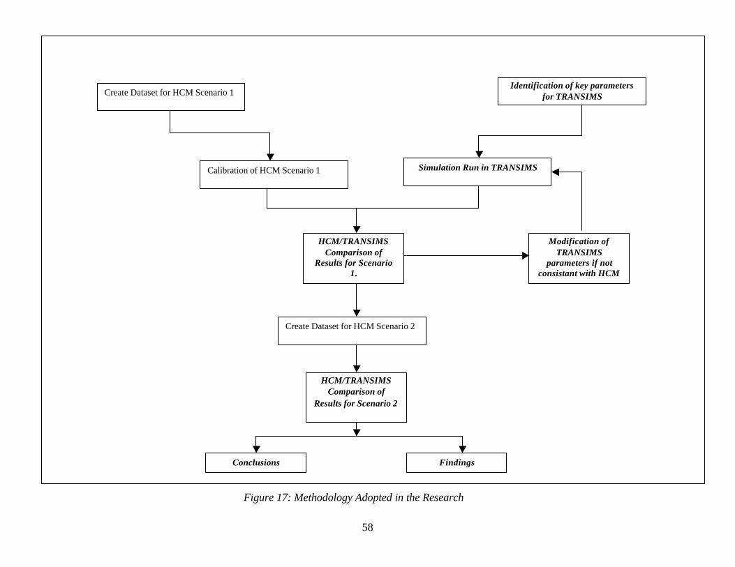
58
Create Dataset for HCM Scenario 1
Create Dataset for HCM Scenario 2
Calibration of HCM Scenario 1
Identification of key parameters for TRANSIMS
HCM/TRANSIMS Comparison of
Results for Scenario 1.
Simulation Run in TRANSIMS
Modification of TRANSIMS
parameters if not consistant with HCM
HCM/TRANSIMS Comparison of
Results for Scenario 2
Conclusions Findings
Figure 17: Methodology Adopted in the Research
59
4.3 The Modeling Concept
The traditional models in HCM predict volumes immediately upstream of the ramp
junction. This prediction is based upon full hour volumes and is done in mixed vehicles
per hour (vph). These models, while simple and straightforward in prediction of volume
become complex when applied to capacity analysis.
In the context of the proposed model construct, several changes have been made to
incorporate a similar model existing in HCM.
• Traditional HCM models focus on volume as input and get speed as an output for the
entire weaving section.
• The HCM is based upon analysis of flow rates within 15-minutes periods of time. To
conform to other methodologies in HCM, 15-minute data periods were used in all the
models studied.
• The calibrations for scenario 1 were made in passenger car equivalents (pce’s), while
Scenario 2 used mixed traffic for analysis purpose.
60
4.4 Modeling in TRANSIMS
4.4.1 Assumptions made in TRANSIMS Some of the standard assumptions made in TRANSIMS
• The link is divided into 7.5-meter cells.
• The vehicles moving on the links are of the types specified by the vehicle prototype
file. They comprise of autos that occupy one cell or trucks that occupy two cells. The
file also states their maximum acceleration and speeds possible.
• The HCM manual specifies the weaving speed and non-weaving speed per vehicle
and all the result that is output from the Microsimulator is the snapshot data. This
snapshot data is interpreted to get all other results.
4.4.2 General Modeling Strategy used in TRANSIMS
To develop a similar scenario as the highway capacity manual, all the necessary tables in
the network were coded manually. The network was split into a combination of nodes
and links with parking at each entry and exit point of the links from where vehicles are
generated and absorbed. Travel plans for each, weaving and nonweaving movements are
generated for the necessary volume to be simulated. The lane, which connects the on-
ramp and the off-ramp on each lane of the weaving link, is modeled as a full-length
auxiliary lane. The rates at which vehicles are generated at the entry links follow a
random normal distribution.
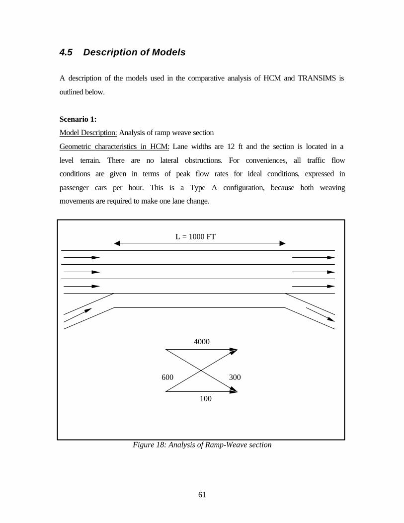
61
4.5 Description of Models
A description of the models used in the comparative analysis of HCM and TRANSIMS is
outlined below.
Scenario 1:
Model Description: Analysis of ramp weave section
Geometric characteristics in HCM: Lane widths are 12 ft and the section is located in a
level terrain. There are no lateral obstructions. For conveniences, all traffic flow
conditions are given in terms of peak flow rates for ideal conditions, expressed in
passenger cars per hour. This is a Type A configuration, because both weaving
movements are required to make one lane change.
Figure 18: Analysis of Ramp-Weave section
L = 1000 FT
600 300
100
4000
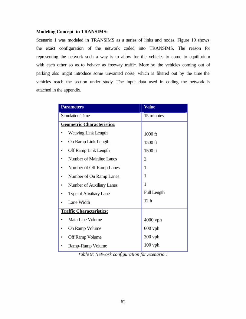
62
Modeling Concept in TRANSIMS:
Scenario 1 was modeled in TRANSIMS as a series of links and nodes. Figure 19 shows
the exact configuration of the network coded into TRANSIMS. The reason for
representing the network such a way is to allow for the vehicles to come to equilibrium
with each other so as to behave as freeway traffic. More so the vehicles coming out of
parking also might introduce some unwanted noise, which is filtered out by the time the
vehicles reach the section under study. The input data used in coding the network is
attached in the appendix.
Parameters Value
Simulation Time 15 minutes
Geometric Characteristics:
• Weaving Link Length
• On Ramp Link Length
• Off Ramp Link Length
• Number of Mainline Lanes
• Number of Off Ramp Lanes
• Number of On Ramp Lanes
• Number of Auxiliary Lanes
• Type of Auxiliary Lane
• Lane Width
1000 ft
1500 ft
1500 ft
3
1
1
1
Full Length
12 ft
Traffic Characteristics:
• Main Line Volume
• On Ramp Volume
• Off Ramp Volume
• Ramp-Ramp Volume
4000 vph
600 vph
300 vph
100 vph
Table 9: Network configuration for Scenario 1
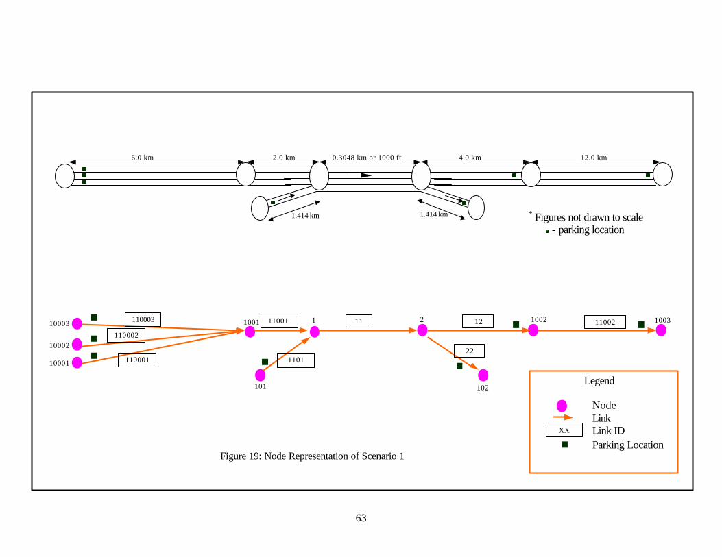
63
Legend Node Link Link ID Parking Location
* Figures not drawn to scale
- parking location
6.0 km 2.0 km 0.3048 km or 1000 ft 4.0 km 12.0 km
1.414 km 1.414 km
10003
10002
10001
1001 1 2 1002 1003
101 102
110003
110002
110001
11001 11
1101
12
22
11002
XX
Figure 19: Node Representation of Scenario 1
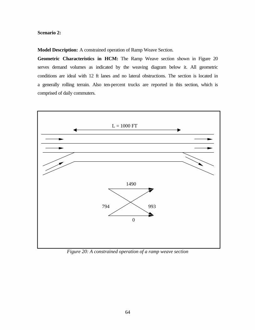
64
Scenario 2:
Model Description: A constrained operation of Ramp Weave Section.
Geometric Characteristics in HCM: The Ramp Weave section shown in Figure 20
serves demand volumes as indicated by the weaving diagram below it. All geometric
conditions are ideal with 12 ft lanes and no lateral obstructions. The section is located in
a generally rolling terrain. Also ten-percent trucks are reported in this section, which is
comprised of daily commuters.
Figure 20: A constrained operation of a ramp weave section
L = 1000 FT
794 993
0
1490
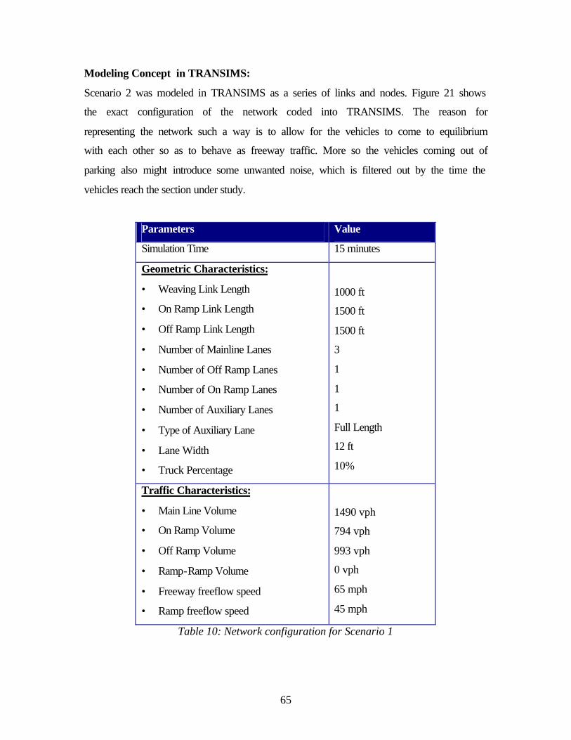
65
Modeling Concept in TRANSIMS:
Scenario 2 was modeled in TRANSIMS as a series of links and nodes. Figure 21 shows
the exact configuration of the network coded into TRANSIMS. The reason for
representing the network such a way is to allow for the vehicles to come to equilibrium
with each other so as to behave as freeway traffic. More so the vehicles coming out of
parking also might introduce some unwanted noise, which is filtered out by the time the
vehicles reach the section under study.
Parameters Value
Simulation Time 15 minutes
Geometric Characteristics:
• Weaving Link Length
• On Ramp Link Length
• Off Ramp Link Length
• Number of Mainline Lanes
• Number of Off Ramp Lanes
• Number of On Ramp Lanes
• Number of Auxiliary Lanes
• Type of Auxiliary Lane
• Lane Width
• Truck Percentage
1000 ft
1500 ft
1500 ft
3
1
1
1
Full Length
12 ft
10%
Traffic Characteristics:
• Main Line Volume
• On Ramp Volume
• Off Ramp Volume
• Ramp-Ramp Volume
• Freeway freeflow speed
• Ramp freeflow speed
1490 vph
794 vph
993 vph
0 vph
65 mph
45 mph
Table 10: Network configuration for Scenario 1

66
Legend Node Link Link ID Parking Location
* Figures not drawn to scale
- parking location
6.0 km 2.0 km 0.3048 km or 1000 ft 4.0 km 12.0 km
1.414 km 1.414 km
10002
10001
1001 1 2 1002 1003
101 102
110002
110001
11001 11
1101
12
22
11002
XX
Figure 21: Node Representation of Scenario 2
67
Chapter 5: Comparing HCM Vs TRANSIMS Results
For the comparison of results between HCM and TRANSIMS it is important to first
create a common data set that could be applied to both models and then results of each
examined and compared to one another.
An important factor for comparison between both the models would be to keep the traffic
conditions similar just before the section under study. HCM does not provide a guideline
to predict the speed and volume of upstream of a ramp. However it can be identified that
this would depend on several parameters such as the type of ramp, total upstream freeway
volume, ramp volume, length, of acceleration lane, anticipatory warning sign distance,
advanced warning sign distance, time to change lanes and freeway flow speed of the
ramp.
A sensitivity analysis is conducted on different parameters to assess the applicability of
TRANSIMS to the existing model in HCM. The following section discusses about these
parameters and the default values used for the scenarios.
5.1 Model Calibration
As there was no field data available to calibrate the simulation model, the HCM results
were used as a baseline for the calibration of TRANSIMS. Although not recommended,
this was done only for the model validation of this experimental study. The following
subsections identify the key parameters or configuration keys and the results of the
sensitivity analysis on them.
5.1.1 Deceleration Probability
The configuration key CA_DECELERATION_PROBABILITY defines the probability of a
driver to decelerate for no reason. This enhances the traffic variation as each automobile
driver randomly decides whether to decelerate for no apparent reason at each timestep.
Since the configuration key defines the probability of a quantity the acceptable values
that can be used for it lie between 0.0 and 1.0.
If the configuration key is set to 0, it would mean that a driver would never decelerate
without a reason. The only time he/she would decelerate would be when the gap ahead of
him/her is less than the velocity at which he/she is driving. If this key is set to 1 it would
68
imply that a driver would always decelerate at every timestep where the gap ahead of
him/her is more than the velocity.
The configuration key is important as it replicates human behavior and tendency to not
accelerate all the time. As stated earlier for a model to depict reality, it is very important
to capture such kind of data and calibrate the model. For the sake of this study, since no
real world data on weaving sections was present. The model was calibrated to that of a
default value of 0.2. This implies that one-fifth of the time a driver would decelerate for
no apparent reason. This value is also justified as the default value was arrived at in
TRANSIMS based on lot of studies conducted by the research team headed by Kai
Nagel.
5.1.2 Lane Change Probability
The configuration key that controls a lane changing maneuver is the
CA_LANE_CHANGE_PROBABILTIY. Should all the conditions be satisfied for a driver to
lane change into the adjacent lane, this configuration key specifies the probability of the
driver to lane change i.e., should a slower vehicle be ahead of a vehicle whose gap ahead
is less than the velocity at which it is traveling and the gap ahead in the adjacent lane is
more than in the current lane while the gap behind in the new lane is more than the
VGlobalMax, then all the conditions are satisfied for a lane change. It should also be noted
that right and left lane changes occur on alternate timesteps. Having all the condition
satisfied for a lane change a driver would still only lane change with a probability given
by this configuration key.
This configuration key is quite crucial for the simulation to be close to reality. An
example to emphasize the importance of this key would be to consider a two lane
roadway with all the vehicles in one lane next to each other. This would mean that every
vehicle would have its conditions for lane change based on gaps fulfilled. So in the next
time step each of the vehicles would move into the adjacent lane. This continues at every
timestep and would result in very unrealistic scenario. Introducing this configuration key
helps stabilize this.
As the configuration key suggests, it represents the probability and so the permissible
values lie between 0 and 1. A default value of 0.99 was arrived at after a lot of
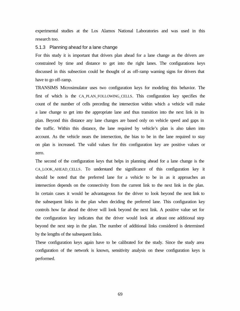
69
experimental studies at the Los Alamos National Laboratories and was used in this
research too.
5.1.3 Planning ahead for a lane change
For this study it is important that drivers plan ahead for a lane change as the drivers are
constrained by time and distance to get into the right lanes. The configurations keys
discussed in this subsection could be thought of as off-ramp warning signs for drivers that
have to go off-ramp.
TRANSIMS Microsimulator uses two configuration keys for modeling this behavior. The
first of which is the CA_PLAN_FOLLOWING_CELLS. This configuration key specifies the
count of the number of cells preceding the intersection within which a vehicle will make
a lane change to get into the appropriate lane and thus transition into the next link in its
plan. Beyond this distance any lane changes are based only on vehicle speed and gaps in
the traffic. Within this distance, the lane required by vehicle’s plan is also taken into
account. As the vehicle nears the intersection, the bias to be in the lane required to stay
on plan is increased. The valid values for this configuration key are positive values or
zero.
The second of the configuration keys that helps in planning ahead for a lane change is the
CA_LOOK_AHEAD_CELLS. To understand the significance of this configuration key it
should be noted that the preferred lane for a vehicle to be in as it approaches an
intersection depends on the connectivity from the current link to the next link in the plan.
In certain cases it would be advantageous for the driver to look beyond the next link to
the subsequent links in the plan when deciding the preferred lane. This configuration key
controls how far ahead the driver will look beyond the next link. A positive value set for
the configuration key indicates that the driver would look at atleast one additional step
beyond the next step in the plan. The number of additional links considered is determined
by the lengths of the subsequent links.
These configuration keys again have to be calibrated for the study. Since the study area
configuration of the network is known, sensitivity analysis on these configuration keys is
performed.
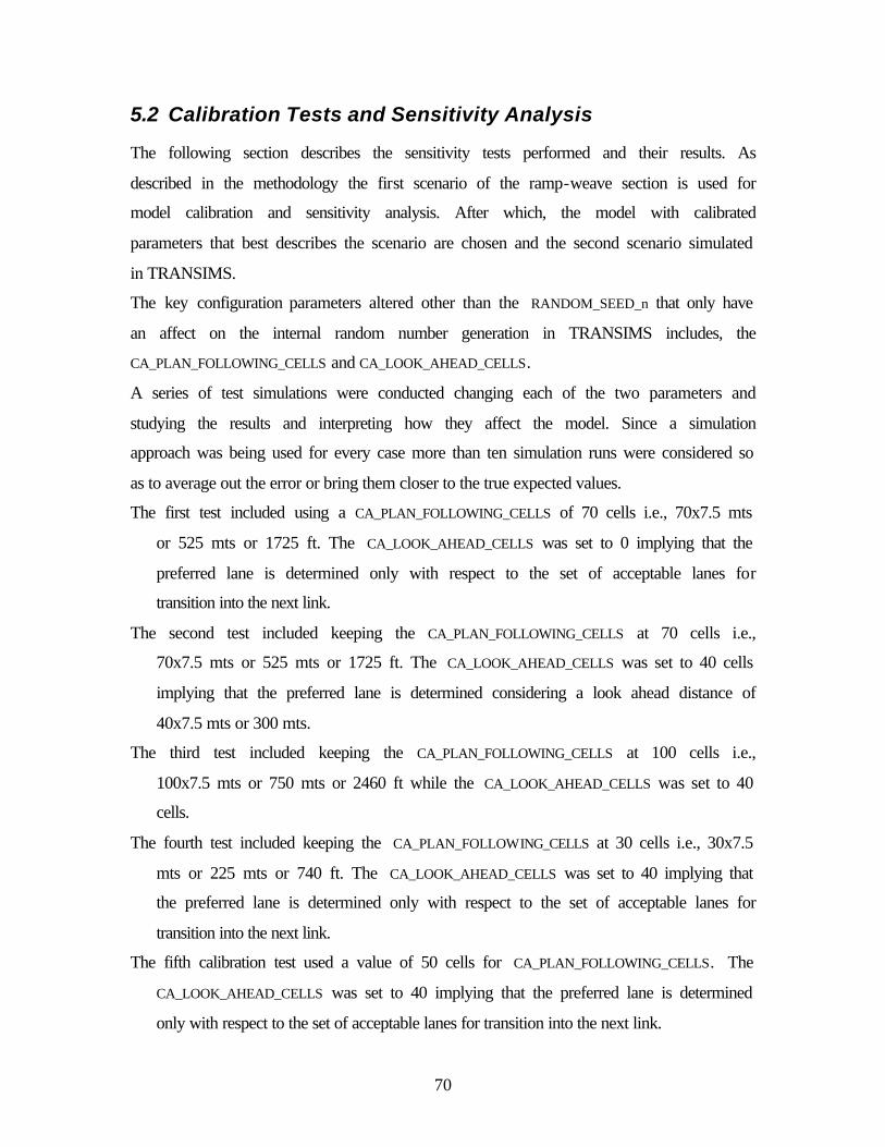
70
5.2 Calibration Tests and Sensitivity Analysis
The following section describes the sensitivity tests performed and their results. As
described in the methodology the first scenario of the ramp-weave section is used for
model calibration and sensitivity analysis. After which, the model with calibrated
parameters that best describes the scenario are chosen and the second scenario simulated
in TRANSIMS.
The key configuration parameters altered other than the RANDOM_SEED_n that only have
an affect on the internal random number generation in TRANSIMS includes, the
CA_PLAN_FOLLOWING_CELLS and CA_LOOK_AHEAD_CELLS.
A series of test simulations were conducted changing each of the two parameters and
studying the results and interpreting how they affect the model. Since a simulation
approach was being used for every case more than ten simulation runs were considered so
as to average out the error or bring them closer to the true expected values.
The first test included using a CA_PLAN_FOLLOWING_CELLS of 70 cells i.e., 70x7.5 mts
or 525 mts or 1725 ft. The CA_LOOK_AHEAD_CELLS was set to 0 implying that the
preferred lane is determined only with respect to the set of acceptable lanes for
transition into the next link.
The second test included keeping the CA_PLAN_FOLLOWING_CELLS at 70 cells i.e.,
70x7.5 mts or 525 mts or 1725 ft. The CA_LOOK_AHEAD_CELLS was set to 40 cells
implying that the preferred lane is determined considering a look ahead distance of
40x7.5 mts or 300 mts.
The third test included keeping the CA_PLAN_FOLLOWING_CELLS at 100 cells i.e.,
100x7.5 mts or 750 mts or 2460 ft while the CA_LOOK_AHEAD_CELLS was set to 40
cells.
The fourth test included keeping the CA_PLAN_FOLLOWING_CELLS at 30 cells i.e., 30x7.5
mts or 225 mts or 740 ft. The CA_LOOK_AHEAD_CELLS was set to 40 implying that
the preferred lane is determined only with respect to the set of acceptable lanes for
transition into the next link.
The fifth calibration test used a value of 50 cells for CA_PLAN_FOLLOWING_CELLS. The
CA_LOOK_AHEAD_CELLS was set to 40 implying that the preferred lane is determined
only with respect to the set of acceptable lanes for transition into the next link.
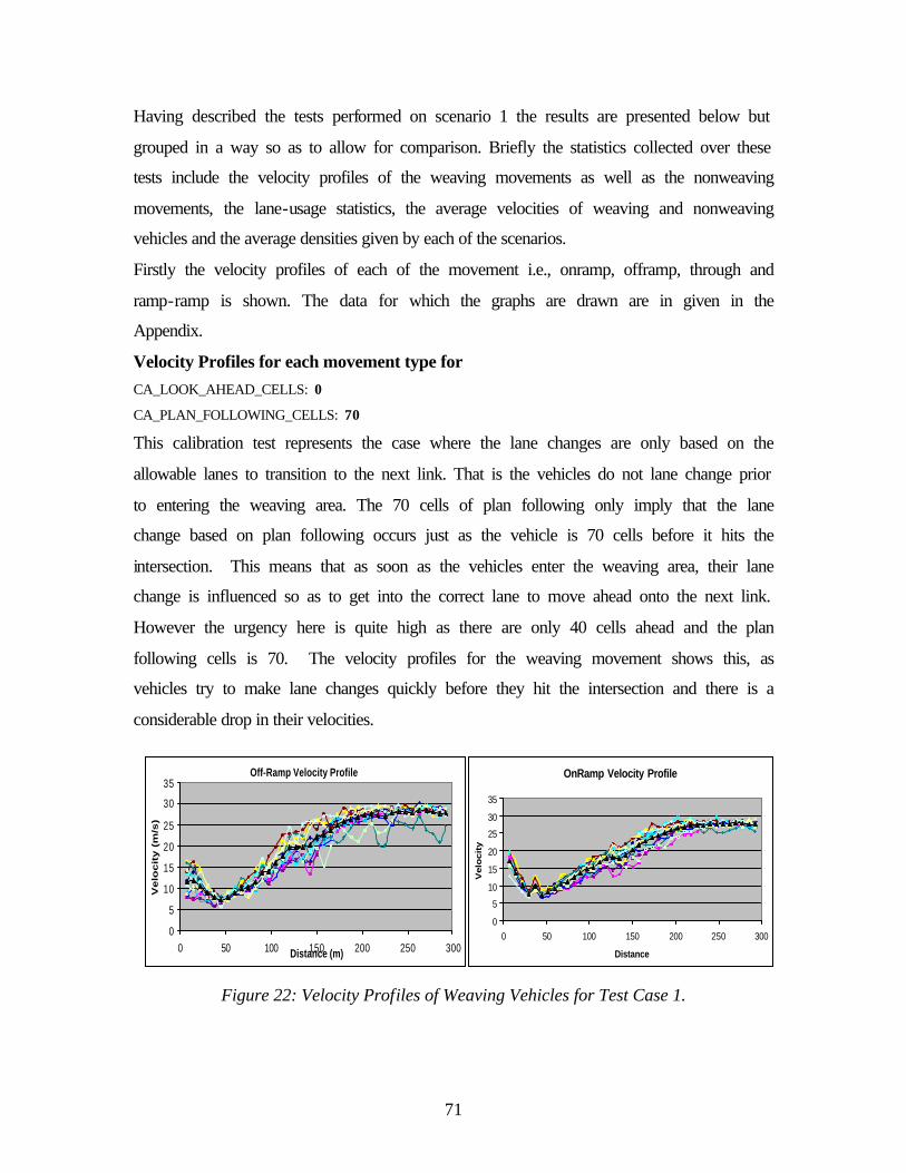
71
Having described the tests performed on scenario 1 the results are presented below but
grouped in a way so as to allow for comparison. Briefly the statistics collected over these
tests include the velocity profiles of the weaving movements as well as the nonweaving
movements, the lane-usage statistics, the average velocities of weaving and nonweaving
vehicles and the average densities given by each of the scenarios.
Firstly the velocity profiles of each of the movement i.e., onramp, offramp, through and
ramp-ramp is shown. The data for which the graphs are drawn are in given in the
Appendix.
Velocity Profiles for each movement type for CA_LOOK_AHEAD_CELLS: 0
CA_PLAN_FOLLOWING_CELLS: 70
This calibration test represents the case where the lane changes are only based on the
allowable lanes to transition to the next link. That is the vehicles do not lane change prior
to entering the weaving area. The 70 cells of plan following only imply that the lane
change based on plan following occurs just as the vehicle is 70 cells before it hits the
intersection. This means that as soon as the vehicles enter the weaving area, their lane
change is influenced so as to get into the correct lane to move ahead onto the next link.
However the urgency here is quite high as there are only 40 cells ahead and the plan
following cells is 70. The velocity profiles for the weaving movement shows this, as
vehicles try to make lane changes quickly before they hit the intersection and there is a
considerable drop in their velocities.
Figure 22: Velocity Profiles of Weaving Vehicles for Test Case 1.
Off-Ramp Velocity Profile
0
5
10
15
20
25
30
35
0 50 100 150 200 250 300Distance (m)
Velo
cit
y (
m/s
)
OnRamp Velocity Profile
0
5
10
15
20
25
30
35
0 50 100 150 200 250 300
Distance
Velo
cit
y
72
For the nonweaving flows i.e., the through traveling vehicles and the ramp-ramp flows,
they should not be much affected because their current lane is a good and an acceptable
lane. The velocities tend to lower near the beginning because of the weaving flows trying
to get into their right lanes. Figure 23 below shows the ramp-ramp and the through
vehicles velocity profiles.
Figure 23: Velocity Profiles of Nonweaving Vehicles for Test Case 1.
Velocity Profiles for each movement type for
CA_LOOK_AHEAD_CELLS: 40
CA_PLAN_FOLLOWING_CELLS: 70
This calibration test exactly the same as the one described above, the only difference
being that the lane changes are now also done looking at the allowable lanes the vehicle
has to be to transition from the next link onto the next. Figure 24 shows the weaving
vehicles velocity profiles, which are not very different from the one above, but the
average vehicle velocities are a bit higher at each distance.
Figure 24: Velocity Profiles of Weaving Vehicles for Test Case 2.
Thru Velocity Profile
0
5
10
15
20
25
30
35
0 50 100 150 200 250 300
Distance
Ve
loc
ity
RampRamp Velocity Profile
0
5
10
15
20
25
30
35
0 50 100 150 200 250 300
Distance (m)V
elo
cit
y (
m/s
)
OffRamp Velocity Profile
0
5
10
15
20
25
30
35
0 50 100 150 200 250 300
distance (m)
ve
loc
ity
(m
/s)
OnRamp Velocity Profile
0
5
10
15
20
25
30
35
0 50 100 150 200 250 300
Distance (m)
Velo
cit
y (m
/s)
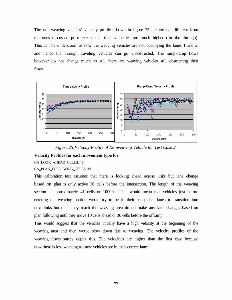
73
The non-weaving vehicles’ velocity profiles shown in figure 25 are too not different from
the ones discussed prior except that their velocities are much higher (for the through).
This can be understood as now the weaving vehicles are not occupying the lanes 1 and 2
and hence the through traveling vehicles can go unobstructed. The ramp-ramp flows
however do not change much as still there are weaving vehicles still obstructing their
flows.
Figure 25:Velocity Profile of Nonweaving Vehicle for Test Case 2.
Velocity Profiles for each movement type for CA_LOOK_AHEAD_CELLS: 40
CA_PLAN_FOLLOWING_CELLS: 30
This calibration test assumes that there is looking ahead across links but lane change
based on plan is only active 30 cells before the intersection. The length of the weaving
section is approximately 41 cells or 1000ft. This would mean that vehicles just before
entering the weaving section would try to be in their acceptable lanes to transition into
next links but once they reach the weaving area do no make any lane changes based on
plan following until they move 10 cells ahead or 30 cells before the offramp.
This would suggest that the vehicles initially have a high velocity at the beginning of the
weaving area and then would slow down due to weaving. The velocity profiles of the
weaving flows surely depict this. The velocities are higher than the first case because
now there is less weaving as most vehicles are in their correct lanes.
Thru Velocity Profile
0
5
10
15
20
25
30
35
0 50 100 150 200 250 300
Distance (m)
Ve
loc
ity
(m
/s)
Ramp-Ramp Velocity Profile
0
5
10
15
20
25
30
35
0 50 100 150 200 250 300
Distance (m)
Velo
cit
y (m
/s)
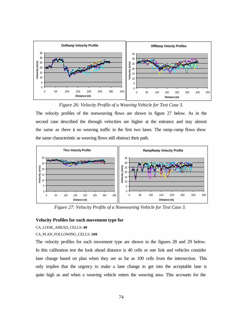
74
Figure 26: Velocity Profile of a Weaving Vehicle for Test Case 3.
The velocity profiles of the nonweaving flows are shown in figure 27 below. As in the
second case described the through velocities are higher at the entrance and stay almost
the same as there is no weaving traffic in the first two lanes. The ramp-ramp flows show
the same characteristic as weaving flows still obstruct their path.
Velocity Profiles for each movement type for CA_LOOK_AHEAD_CELLS: 40
CA_PLAN_FOLLOWING_CELLS: 100
The velocity profiles for each movement type are shown in the figures 28 and 29 below.
In this calibration test the look ahead distance is 40 cells or one link and vehicles consider
lane change based on plan when they are as far as 100 cells from the intersection. This
only implies that the urgency to make a lane change to get into the acceptable lane is
quite high as and when a weaving vehicle enters the weaving area. This accounts for the
OnRamp Velocity Profile
0
5
10
15
20
25
30
35
0 50 100 150 200 250 300 350
Distance (m)
Vel
oci
ty (m
/s)
OffRamp Velocity Profiles
0
5
10
15
20
25
30
35
0 50 100 150 200 250 300 350
Distance (m)
Velo
cit
y (
m/s
)
Thru Velocity Profile
0
5
10
15
20
25
30
0 50 100 150 200 250 300 350
Distance (m)
Velo
cit
y (
m/s
)
RampRamp Velocity Profile
0
5
10
15
20
25
30
35
0 50 100 150 200 250 300 350
Distance (m)
Velo
cit
y (
m/s
)
Figure 27: Velocity Profile of a Nonweaving Vehicle for Test Case 3.
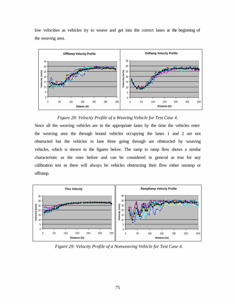
75
low velocities as vehicles try to weave and get into the correct lanes at the beginning of
the weaving area.
Figure 28: Velocity Profile of a Weaving Vehicle for Test Case 4.
Since all the weaving vehicles are in the appropriate lanes by the time the vehicles enter
the weaving area the through bound vehicles occupying the lanes 1 and 2 are not
obstructed but the vehicles in lane three going through are obstructed by weaving
vehicles, which is shown in the figures below. The ramp to ramp flow shows a similar
characteristic as the ones before and can be considered in general as true for any
calibration test as there will always be vehicles obstructing their flow either onramp or
offramp.
OffRamp Velocity Profile
0
5
10
15
20
25
30
35
0 50 100 150 200 250 300
Distance (m)
Velo
cit
y (
m/s
)
OnRamp Velocity Profile
0
5
10
15
20
25
30
35
0 50 100 150 200 250 300
Distance (m)
Ve
loc
ity
(m
/s)
Thru Velocity
0
5
10
15
20
25
30
35
0 50 100 150 200 250 300
Distance (m)
Velo
cit
y (m
/s)
RampRamp Velocity Profile
0
5
10
15
20
25
30
35
0 50 100 150 200 250 300
Distance (m)
Velo
cit
y (
m/s
)
Figure 29: Velocity Profile of a Nonweaving Vehicle for Test Case 4.

76
Time-Space diagrams for a typical vehicle by movement type:
Having looked at the velocity profiles for the different vehicles, a better understanding of
the particle hopping theory as well as the actual movements of the vehicles could be
understood with time-space figures. The time-space diagrams for the four test scenarios
are presented below and since the distance of vehicle movements is closely related to the
velocity, a plot of the velocity on the same figure is shown. The data for which these
figures are plotted are attached in the Appendix B.
Figure 30: Time-Space Diagrams for a single Ramp-Ramp moving vehicle
The figures shown above depict a single vehicles path as it traverses the weaving section.
The x-axis on these graphs represents the time. It is assumed that the time at which the
vehicle enters the weaving section is 0 and the trajectory is presented till the time it
moves off the weaving section. The data are shown in points in accordance with the
cellular automata and particle hopping theory.
Ramp-Ramp Test 1
0
50
100
150
200
250
300
0 2 4 6 8 10 12 14 16 18
Time
Dis
tan
ce (
m);
Sp
eed
(m
/s)
Distance
Speed
Ramp-Ramp Test 2
0
50
100
150
200
250
300
0 5 10 15 20 25
Time
Dis
tan
ce(m
); S
pee
d (
m/s
)distance
speed
Ramp-Ramp Test 3
0
50
100
150
200
250
300
350
0 2 4 6 8 10 12
Time
Dis
tan
ce (
m);
Sp
eed
(m
/s)
distance
speed
Ramp-Ramp Test 4
0
50
100
150
200
250
300
0 2 4 6 8 10
Time
Dis
tan
ce (
m);
Sp
eed
(m
/s)
distance
speed

77
Figure 31: Time-Space Diagrams for a single through vehicle.
Figure 32: Time-Space Diagrams for a single Offramp vehicle.
Offramp Test 1
0
50
100
150
200
250
300
0 2 4 6 8 10 12 14 16 18
Time
Dis
tanc
e(m
); S
peed
(m/s
)
Distance
Speed
Offramp Test 2
0
50
100
150
200
250
300
0 2 4 6 8 10 12 14 16
Time
Dis
tanc
e(m
); S
peed
(m
/s)
distance
speed
Offramp Test 3
0
50
100
150
200
250
300
0 5 10 15 20
Time
Dis
tanc
e (m
); S
peed
(m
/s)
distancespeed
Offramp Test 4
0
50
100
150
200
250
300
0 5 10 15 20 25
Time
Dis
tanc
e (m
); S
peed
(m/s
)
distance
speed
Through Test 1 (lane 4)
0
50
100
150
200
250
300
0 5 10 15 20
Time
Dis
tanc
e(m
); S
peed
(m
/s)
Distance
Speed
Through Test 2
0
50
100
150
200
250
300
350
0 2 4 6 8 10 12
Time
Dis
tanc
e (m
); S
peed
(m/s
)
distance
speed
Through Test 3
0
50
100
150
200
250
300
350
0 2 4 6 8 10 12 14
Time
Dis
tanc
e(m
); S
peed
(m/s
)
distance
speed
Through Test 4
0
50
100
150
200
250
300
0 2 4 6 8 10 12 14 16
Time
Dis
tanc
e(m
); S
peed
(m
/s)
distance
speed
(Lane 3)
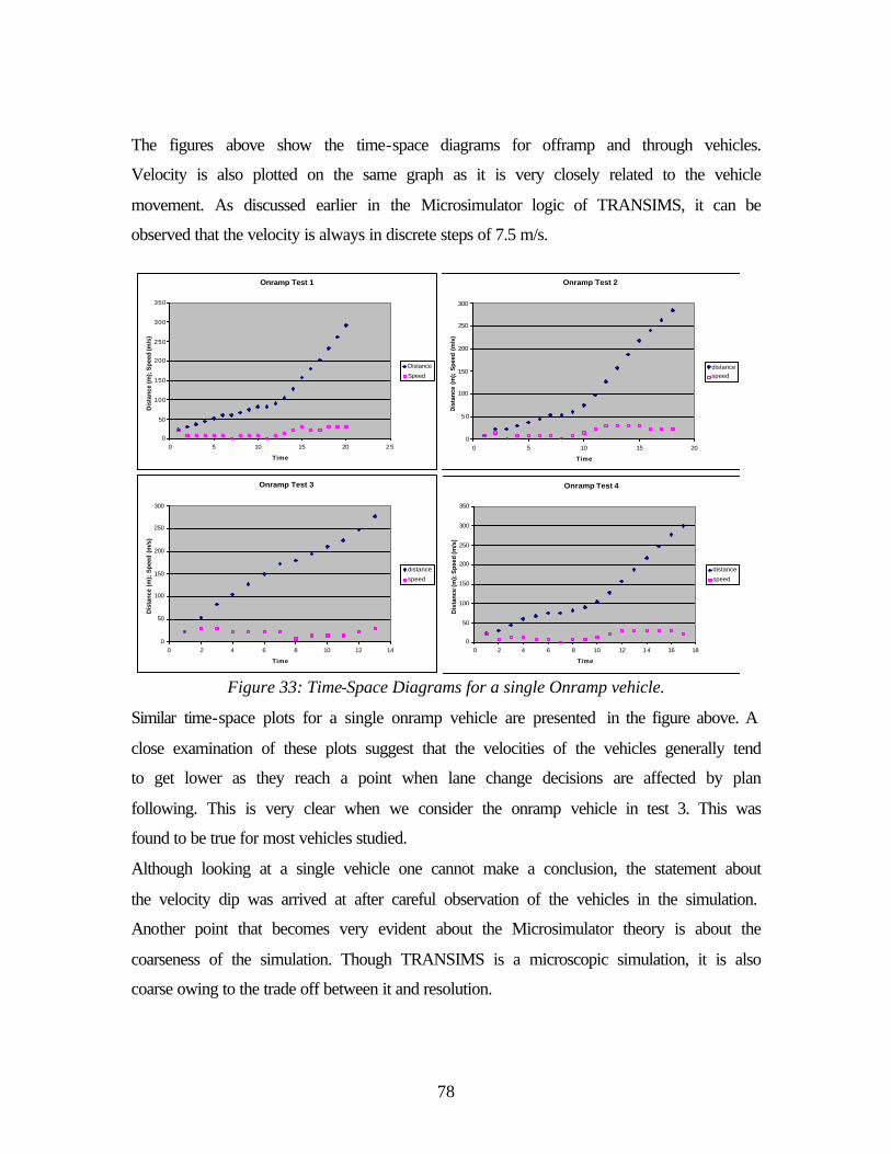
78
The figures above show the time-space diagrams for offramp and through vehicles.
Velocity is also plotted on the same graph as it is very closely related to the vehicle
movement. As discussed earlier in the Microsimulator logic of TRANSIMS, it can be
observed that the velocity is always in discrete steps of 7.5 m/s.
Figure 33: Time-Space Diagrams for a single Onramp vehicle.
Similar time-space plots for a single onramp vehicle are presented in the figure above. A
close examination of these plots suggest that the velocities of the vehicles generally tend
to get lower as they reach a point when lane change decisions are affected by plan
following. This is very clear when we consider the onramp vehicle in test 3. This was
found to be true for most vehicles studied.
Although looking at a single vehicle one cannot make a conclusion, the statement about
the velocity dip was arrived at after careful observation of the vehicles in the simulation.
Another point that becomes very evident about the Microsimulator theory is about the
coarseness of the simulation. Though TRANSIMS is a microscopic simulation, it is also
coarse owing to the trade off between it and resolution.
Onramp Test 1
0
50
100
150
200
250
300
350
0 5 10 15 20 25
Time
Dis
tanc
e (m
); S
peed
(m/s
)
Distance
Speed
Onramp Test 2
0
50
100
150
200
250
300
0 5 10 15 20
TimeD
ista
nce
(m);
Spe
ed (
m/s
)
distancespeed
Onramp Test 3
0
50
100
150
200
250
300
0 2 4 6 8 10 12 14
Time
Dis
tanc
e (m
); S
peed
(m
/s)
distance
speed
Onramp Test 4
0
50
100
150
200
250
300
350
0 2 4 6 8 10 12 14 16 18
Time
Dis
tanc
e (m
); S
peed
(m/s
)
distance
speed
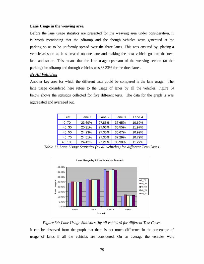
79
Lane Usage in the weaving area:
Before the lane usage statistics are presented for the weaving area under consideration, it
is worth mentioning that the offramp and the though vehicles were generated at the
parking so as to be uniformly spread over the three lanes. This was ensured by placing a
vehicle as soon as it is created on one lane and making the next vehicle go into the next
lane and so on. This means that the lane usage upstream of the weaving section (at the
parking) for offramp and through vehicles was 33.33% for the three lanes.
By All Vehicles:
Another key area for which the different tests could be compared is the lane usage. The
lane usage considered here refers to the usage of lanes by all the vehicles. Figure 34
below shows the statistics collected for five different tests. The data for the graph is was
aggregated and averaged out.
Test Lane 1 Lane 2 Lane 3 Lane 4
0_70 23.69% 27.86% 37.65% 10.69% 40_30 25.31% 27.06% 35.55% 11.97%
40_50 24.93% 27.30% 36.67% 10.99%
40_70 24.51% 27.30% 37.29% 10.79% 40_100 24.42% 27.21% 36.98% 11.27%
Table 11:Lane Usage Statistics (by all vehicles) for different Test Cases.
Figure 34: Lane Usage Statistics (by all vehicles) for different Test Cases.
It can be observed from the graph that there is not much difference in the percentage of
usage of lanes if all the vehicles are considered. On an average the vehicles were
Lane Usage by All Vehicles Vs Scenario
0.00%
5.00%
10.00%
15.00%
20.00%
25.00%
30.00%
35.00%
40.00%
Lane 1 Lane 2 Lane 3 Lane 4
Scenario
Lane
Usa
ge % 0_70
40_30
40_50
40_70
40_100
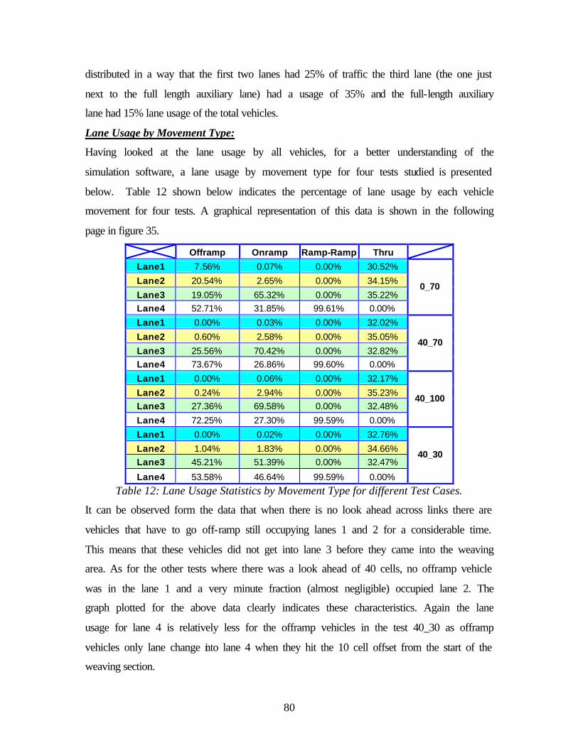
80
distributed in a way that the first two lanes had 25% of traffic the third lane (the one just
next to the full length auxiliary lane) had a usage of 35% and the full-length auxiliary
lane had 15% lane usage of the total vehicles.
Lane Usage by Movement Type:
Having looked at the lane usage by all vehicles, for a better understanding of the
simulation software, a lane usage by movement type for four tests studied is presented
below. Table 12 shown below indicates the percentage of lane usage by each vehicle
movement for four tests. A graphical representation of this data is shown in the following
page in figure 35.
Offramp Onramp Ramp-Ramp Thru
Lane1 7.56% 0.07% 0.00% 30.52%
Lane2 20.54% 2.65% 0.00% 34.15%
Lane3 19.05% 65.32% 0.00% 35.22% Lane4 52.71% 31.85% 99.61% 0.00%
0_70
Lane1 0.00% 0.03% 0.00% 32.02%
Lane2 0.60% 2.58% 0.00% 35.05%
Lane3 25.56% 70.42% 0.00% 32.82% Lane4 73.67% 26.86% 99.60% 0.00%
40_70
Lane1 0.00% 0.06% 0.00% 32.17%
Lane2 0.24% 2.94% 0.00% 35.23% Lane3 27.36% 69.58% 0.00% 32.48%
Lane4 72.25% 27.30% 99.59% 0.00%
40_100
Lane1 0.00% 0.02% 0.00% 32.76%
Lane2 1.04% 1.83% 0.00% 34.66% Lane3 45.21% 51.39% 0.00% 32.47%
Lane4 53.58% 46.64% 99.59% 0.00%
40_30
Table 12: Lane Usage Statistics by Movement Type for different Test Cases.
It can be observed form the data that when there is no look ahead across links there are
vehicles that have to go off-ramp still occupying lanes 1 and 2 for a considerable time.
This means that these vehicles did not get into lane 3 before they came into the weaving
area. As for the other tests where there was a look ahead of 40 cells, no offramp vehicle
was in the lane 1 and a very minute fraction (almost negligible) occupied lane 2. The
graph plotted for the above data clearly indicates these characteristics. Again the lane
usage for lane 4 is relatively less for the offramp vehicles in the test 40_30 as offramp
vehicles only lane change into lane 4 when they hit the 10 cell offset from the start of the
weaving section.
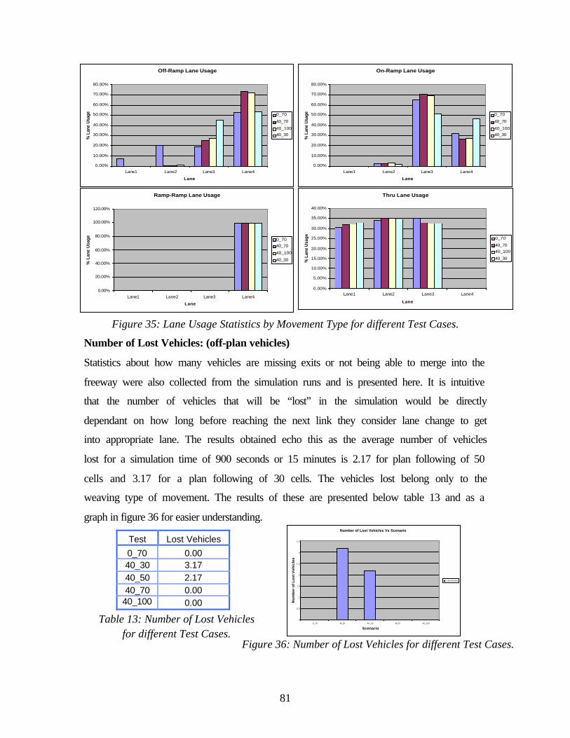
81
Figure 35: Lane Usage Statistics by Movement Type for different Test Cases.
Number of Lost Vehicles: (off-plan vehicles)
Statistics about how many vehicles are missing exits or not being able to merge into the
freeway were also collected from the simulation runs and is presented here. It is intuitive
that the number of vehicles that will be “lost” in the simulation would be directly
dependant on how long before reaching the next link they consider lane change to get
into appropriate lane. The results obtained echo this as the average number of vehicles
lost for a simulation time of 900 seconds or 15 minutes is 2.17 for plan following of 50
cells and 3.17 for a plan following of 30 cells. The vehicles lost belong only to the
weaving type of movement. The results of these are presented below table 13 and as a
graph in figure 36 for easier understanding.
Test Lost Vehicles
0_70 0.00 40_30 3.17 40_50 2.17 40_70 0.00
40_100 0.00
Off-Ramp Lane Usage
0.00%
10.00%
20.00%
30.00%
40.00%
50.00%
60.00%
70.00%
80.00%
Lane1 Lane2 Lane3 Lane4
Lane
% L
ane
Usa
ge 0_70
40_70
40_10040_30
On-Ramp Lane Usage
0.00%
10.00%
20.00%
30.00%
40.00%
50.00%
60.00%
70.00%
80.00%
Lane1 Lane2 Lane3 Lane4
Lane
% L
ane
Usa
ge 0_70
40_70
40_10040_30
Ramp-Ramp Lane Usage
0.00%
20.00%
40.00%
60.00%
80.00%
100.00%
120.00%
Lane1 Lane2 Lane3 Lane4
Lane
% L
ane
Usa
ge 0_7040_70
40_100
40_30
Thru Lane Usage
0.00%
5.00%
10.00%
15.00%
20.00%
25.00%
30.00%
35.00%
40.00%
Lane1 Lane2 Lane3 Lane4
Lane%
Lan
e U
sage 0_70
40_70
40_100
40_30
Number of Lost Vehicles Vs Scenario
0
0.5
1
1.5
2
2.5
3
3.5
0_70 40_30 40_50 40_70 40_100
Scenario
Nu
mb
er o
f L
ost
Veh
icle
s
Lost Vehicles
Figure 36: Number of Lost Vehicles for different Test Cases.
Table 13: Number of Lost Vehicles for different Test Cases.
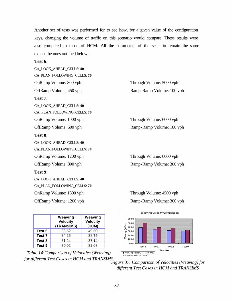
82
Another set of tests was performed for to see how, for a given value of the configuration
keys, changing the volume of traffic on this scenario would compare. These results were
also compared to those of HCM. All the parameters of the scenario remain the same
expect the ones outlined below.
Test 6:
CA_LOOK_AHEAD_CELLS: 40
CA_PLAN_FOLLOWING_CELLS: 70
OnRamp Volume: 800 vph Through Volume: 5000 vph
OffRamp Volume: 450 vph Ramp-Ramp Volume: 100 vph
Test 7:
CA_LOOK_AHEAD_CELLS: 40
CA_PLAN_FOLLOWING_CELLS: 70
OnRamp Volume: 1000 vph Through Volume: 6000 vph
OffRamp Volume: 600 vph Ramp-Ramp Volume: 100 vph
Test 8:
CA_LOOK_AHEAD_CELLS: 40
CA_PLAN_FOLLOWING_CELLS: 70
OnRamp Volume: 1200 vph Through Volume: 6000 vph
OffRamp Volume: 800 vph Ramp-Ramp Volume: 300 vph
Test 9: CA_LOOK_AHEAD_CELLS: 40
CA_PLAN_FOLLOWING_CELLS: 70
OnRamp Volume: 1800 vph Through Volume: 4500 vph
OffRamp Volume: 1200 vph Ramp-Ramp Volume: 300 vph
Weaving Velocity
(TRANSIMS)
Weaving Velocity (HCM)
Test 6 38.52 49.50 Test 7 34.26 38.75 Test 8 31.24 37.14 Test 9 30.02 32.03
Table 14:Comparison of Velocities (Weaving) for different Test Cases in HCM and TRANSIMS
Figure 37: Comparison of Velocities (Weaving) for different Test Cases in HCM and TRANSIMS
Weaving Velocity Comparison
0.00
10.00
20.00
30.00
40.00
50.00
60.00
Test 6 Test 7 Test 8 Test 9
Test No
Velo
city
(mi/h
r)
Weaving Velocity (TRANSIMS)Weaving Velocity (HCM)
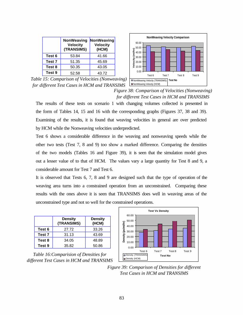
83
NonWeaving
Velocity (TRANSIMS)
NonWeaving Velocity (HCM)
Test 6 53.84 41.66 Test 7 51.35 45.69 Test 8 50.35 43.05 Test 9 52.58 43.72
The results of these tests on scenario 1 with changing volumes collected is presented in
the form of Tables 14, 15 and 16 with the corresponding graphs (Figures 37, 38 and 39).
Examining of the results, it is found that weaving velocities in general are over predicted
by HCM while the Nonweaving velocities underpredicted.
Test 6 shows a considerable difference in the weaving and nonweaving speeds while the
other two tests (Test 7, 8 and 9) too show a marked difference. Comparing the densities
of the two models (Tables 16 and Figure 39), it is seen that the simulation model gives
out a lesser value of to that of HCM. The values vary a large quantity for Test 8 and 9, a
considerable amount for Test 7 and Test 6.
It is observed that Tests 6, 7, 8 and 9 are designed such that the type of operation of the
weaving area turns into a constrained operation from an unconstrained. Comparing these
results with the ones above it is seen that TRANSIMS does well in weaving areas of the
unconstrained type and not so well for the constrained operations.
Density
(TRANSIMS) Density (HCM)
Test 6 27.72 33.26 Test 7 31.13 43.69 Test 8 34.05 48.89 Test 9 35.82 50.86
Figure 38: Comparison of Velocities (Nonweaving) for different Test Cases in HCM and TRANSIMS
Table 15: Comparison of Velocities (Nonweaving) for different Test Cases in HCM and TRANSIMS
NonWeaving Velocity Comparison
0.00
10.00
20.00
30.00
40.00
50.00
60.00
Test 6 Test 7 Test 8 Test 9
Test No
Ve
loc
ity
(m
i/h
r)
NonWeaving Velocity (TRANSIMS)NonWeaving Velocity (HCM)
Figure 39: Comparison of Densities for different Test Cases in HCM and TRANSIMS
Table 16:Comparision of Densities for different Test Cases in HCM and TRANSIMS
Test Vs Density
0.00
10.00
20.00
30.00
40.00
50.00
60.00
Test 6 Test 7 Test 8 Test 9
Test No
Den
sity
(pc/
mi/h
r)
Density (TRANSIMS)
Density (HCM)
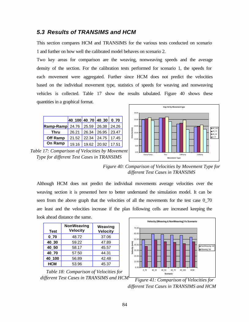
84
5.3 Results of TRANSIMS and HCM
This section compares HCM and TRANSIMS for the various tests conducted on scenario
1 and further on how well the calibrated model behaves on scenario 2.
Two key areas for comparison are the weaving, nonweaving speeds and the average
density of the section. For the calibration tests performed for scenario 1, the speeds for
each movement were aggregated. Further since HCM does not predict the velocities
based on the individual movement type, statistics of speeds for weaving and nonweaving
vehicles is collected. Table 17 show the results tabulated. Figure 40 shows these
quantities in a graphical format.
40_100 40_70 40_30 0_70
Ramp-Ramp 24.76 25.59 26.38 24.26 Thru 26.21 26.34 26.95 23.47
Off Ramp 21.52 22.34 24.75 17.45 On Ramp 19.16 19.62 20.92 17.51
Although HCM does not predict the individual movements average velocities over the
weaving section it is presented here to better understand the simulation model. It can be
seen from the above graph that the velocities of all the movements for the test case 0_70
are least and the velocities increase if the plan following cells are increased keeping the
look ahead distance the same.
Test NonWeaving
Velocity Weaving Velocity
0_70 48.72 37.06 40_30 59.22 47.89 40_50 58.17 45.57 40_70 57.50 44.31 40_100 56.89 42.48 HCM 53.96 45.37
Velocity (Weaving & NonWeaving) Vs Scenario
0.00
10.00
20.00
30.00
40.00
50.00
60.00
70.00
0_70 40_30 40_50 40_70 40_100 HCM
Scenario
Velo
cit
y (
m/s
)
NonWeaving Vel
Weaving Vel
Figure 41: Comparison of Velocities for different Test Cases in TRANSIMS and HCM
Table 18: Comparison of Velocities for different Test Cases in TRANSIMS and HCM
Table 17: Comparison of Velocities by Movement Type for different Test Cases in TRANSIMS
Avg Vel by Movement type
0.00
5.00
10.00
15.00
20.00
25.00
30.00
Ramp-Ramp Thru OffRamp OnRamp
Movement Type
Vel
oci
ty (m
/s) 40_100
40_70
40_30
0_70
Figure 40: Comparison of Velocities by Movement Type for different Test Cases in TRANSIMS
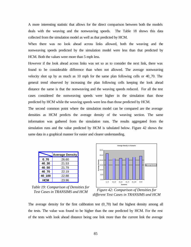
85
A more interesting statistic that allows for the direct comparison between both the models
deals with the weaving and the nonweaving speeds. The Table 18 shows this data
collected from the simulation model as well as that predicted by HCM.
When there was no look ahead across links allowed, both the weaving and the
nonweaving speeds predicted by the simulation model were less than that predicted by
HCM. Both the values were more than 5 mph less.
However if the look ahead across links was set so as to consider the next link, there was
found to be considerable difference than when not allowed. The average nonweaving
velocity shot up by as much as 10 mph for the same plan following cells or 40_70. The
general trend observed by increasing the plan following cells keeping the look ahead
distance the same is that the nonweaving and the weaving speeds reduced. For all the test
cases considered the nonweaving speeds were higher in the simulation than those
predicted by HCM while the weaving speeds were less than those predicted by HCM.
The second common point where the simulation model can be compared are the average
densities as HCM predicts the average density of the weaving section. The same
information was gathered from the simulation runs. The results aggregated from the
simulation runs and the value predicted by HCM is tabulated below. Figure 42 shows the
same data in a graphical manner for easier and clearer understanding.
Average Density
0_70 26.60 40_30 21.53 40_50 21.79 40_70 22.19
40_100 22.88 HCM 23.96
The average density for the first calibration test (0_70) had the highest density among all
the tests. The value was found to be higher than the one predicted by HCM. For the rest
of the tests with look ahead distance being one link more than the current link the average
Average Density vs Scenario
0.00
5.00
10.00
15.00
20.00
25.00
30.00
0_70 40_30 40_50 40_70 40_100 HCM
Scenario
Avera
ge D
en
sit
y
Average Density
Figure 42: Comparison of Densities for different Test Cases in TRANSIMS and HCM
Table 19: Comparison of Densities for Test Cases in TRANSIMS and HCM
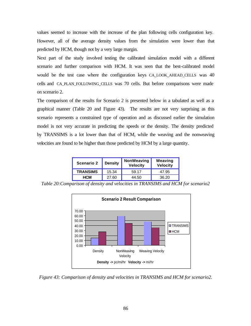
86
values seemed to increase with the increase of the plan following cells configuration key.
However, all of the average density values from the simulation were lower than that
predicted by HCM, though not by a very large margin.
Next part of the study involved testing the calibrated simulation model with a different
scenario and further comparison with HCM. It was seen that the best-calibrated model
would be the test case where the configuration keys CA_LOOK_AHEAD_CELLS was 40
cells and CA_PLAN_FOLLOWING_CELLS was 70 cells. But before comparisons were made
on scenario 2.
The comparison of the results for Scenario 2 is presented below in a tabulated as well as a
graphical manner (Table 20 and Figure 43). The results are not very surprising as this
scenario represents a constrained type of operation and as discussed earlier the simulation
model is not very accurate in predicting the speeds or the density. The density predicted
by TRANSIMS is a lot lower than that of HCM, while the weaving and the nonweaving
velocities are found to be higher than those predicted by HCM by a large quantity.
Scenario 2 Density NonWeaving
Velocity Weaving Velocity
TRANSIMS 15.34 59.17 47.95 HCM 27.60 44.50 36.20
Table 20:Comparison of density and velocities in TRANSIMS and HCM for scenario2
Figure 43: Comparison of density and velocities in TRANSIMS and HCM for scenario2.
Scenario 2 Result Comparison
0.0010.0020.0030.0040.0050.0060.0070.00
Density NonWeavingVelocity
Weaving Velocity
Density -> pc/mi/hr Velocity -> mi/hr
TRANSIMS
HCM

87
Chapter 6: Conclusions
The fundamental difference between HCM and TRANSIMS is that HCM is a
deterministic model in which the results are based on traditional data collected in the
1960’s and revised while TRANSIMS is a stochastic simulation model, which can model
results based on several driver behavior parameters. A 15-minute simulation run only
represents one point of the data sample while HCM may represent an average value of
samples. Although a series of twelve simulation runs were performed for every test and
scenario and an average collected for TRANSIMS, it only reduces the average error and
gets the results closer to the true convergence value of the simulation.
This research evaluates how well TRANSIMS’ ability to replicate complex-weaving
patterns in short distances. The previous chapters have outlined the comparative analysis
and results of weaving areas between TRANSIMS and HCM. In general, the following
conclusions cold be drawn from the basis of the analysis
1) TRANSIMS is not sensitive to various geometric factors such as lane width,
length of acceleration lane, length of deceleration lane etc.
2) It was also found that TRANSIMS results compared fairly well with HCM for
Type A weaving areas under an unconstrained operation but the results did not
match closely with HCM under a constrained operation.
3) The Microsimulator being a microscopic yet a coarse model did not predict the
velocities of individual vehicles along the weaving section very accurately.
Vehicles were found to stop along the weaving section for a second or two, which
is very unlike realistic scenario.
HCM on the other hand was not very useful in predicting the lane usage statistics unlike
most simulation models by which such data could be aggregated. Another key area was
in the prediction of velocities along the section. There was no way of predicting the
velocities across the section for different movement types which can again be collected
from most simulation models.
88
Scope for future research
This research mainly concentrated on comparison of Type A weaving areas, further study
could be conducted on how different the simulation results would be for other types of
configurations. Further research could try to compare a microscopic simulation model to
TRANSIMS and see how the results compare.
Another point of interest is that TRANSIMS does not have logic for deceleration and
acceleration auxiliary lanes. This could be very critical for the consideration of vehicle
emissions. Again, the dealing of TRANSIMS in the deceleration and acceleration of a
vehicle controlled by the configuration keys, does not allow for a change in behavior
depending on the functional class of the road i.e., the same deceleration and acceleration
patters are used for both arterials and freeways. The effectiveness of such an approach or
its deficiencies could be studied.
Bibliography
“A Report on Capacity and Level of Service at Ramp Freeway Junctions” prepared by
Renesselar Polytechnic, New York, 1996
“Center For Microcomputers in Transportation Catalog”, University of Florida
Transportation Research Center, Florida, 1996
Chien, Steven I-Jy and Chowdhury, Shoaib M., "Freeway Capacity Analysis with
Microscopic Simulation Models," Draft Report, Federal Highway Administration, U.S.
Department of Transportation, 1997.
Course Manual on TRANSIMS Microsimulator, Developed at Virginia Tech, 2000.
Essam Radwan, Sylvester A. F. Kalevela “An investigation of the effect of change in
vehicular characteristics on the highway capacity”, Transportation Reset Board,
Washington, D.C., 1975
Finnegan P. and P. Green. “The time to change lanes: A literature review. IVHS”
Technical Report -90-13. US department of Commerce, Sept. 1990
Garber, Nicholas J. And Gadiraju, Ravi, "Factors affecting Speed Variance and Its
Influence on Accidents" Transportation Research Record No. 1213, pp 64-71.
Halati, A., et al., “Lane changing in Freeway Simulation models,” Transportation
Research Board Publication, 1990
Harkey, David L., Robertson, Douglas, and Davis, Scott E., "Assessment of Current
Speed Zoning Criteria," Transportation Research Record No. 1281, Transportation
Research Board, Washington, D. C., 1990.
“Highway Capacity Manual, Special Report 209 ”, Transportation Research Board,
Washington, D. C., 1997.
J.H. Buhr, T.C. Meserole and D.Drew, “ A digital simulation program of a section of
freeway with entrance and exit ramps”, Highway Research Record No. 250, 1968
Jack D. Jernigan and Cheryl W. Lynn “Impact of speed limit on freeway”, Highway
Research Proceedings No. 45, 1996.
Koutsopoullos, H.N., M.E. Ben-Akiva, R.G. Mishalani and K.I. Ahmed. “Modeling
Freeway lane change behavior”. Proceedings of the applications of advanced
technologies in Transportation conference. ASCE, Capri, 1995
May, A.D. “Traffic Flow Fundamentals” Prentice Hall Inc., Englewood Cliffs, NJ, 1990
McShane, William R. and Roess, Roger P., "Traffic Engineering," Prentice Hall press,
1990.
Nemeth, Zoltan A. and Rathi, Ajit K., "Potential impact of speed reduction at freeway
lane closures: A Simulation Study" Transportation Research Record No. 1035, pp 82-84.
Nagel, K. et al, “Two Lane traffic rules for cellular Automata: A systematic approach”,
LA-UR 97-4706, Los Alamos Unclassified Report, Los Alamos National Laboratory, Los
Alamos, NM, USA.
Nagel, K. et al, “TRANSIMS traffic flow characteristics”, LA-UR 97-3531, Los Alamos
Unclassified Report, Los Alamos National Laboratory, Los Alamos, NM, USA.
Nagel, K. et al, “Network Traffic as a self organizing phenomenon”, LA-UR 96-659, Los
Alamos Unclassified Report, Los Alamos National Laboratory, Los Alamos, NM, USA.
Nagel, K., “Particle Hopping Models and Traffic Flow Theory”, LA-UR 95-2908, Los
Alamos Unclassified Report, Los Alamos National Laboratory, Los Alamos, NM, USA.
Nagel, K., “Particle Hopping vs. Fluid-Dynamical Models for Traffic Flow”, LA-UR 95-
4018, Los Alamos Unclassified Report, Los Alamos National Laboratory, Los Alamos,
NM, USA.
Rickert, M., K.Nagel et al, “Two lane simulations using cellular automata”. Technical
Draft, Nov. 1995.
Simon P and Nagel K, “A simplified Cellular Automaton Model for City Traffic”, LA-
UR 97-4707, Los Alamos Unclassified Report, Los Alamos National Laboratory, Los
Alamos, NM, USA.
Suresh Ramachandran, Hobeika A., “Analysis of freeway weaving areas under corridor
simulator and Highway Capacity Manual”, Masters Thesis, Virginia Polytechnic Institute
and State University, November 1997.
TRANSIMS website, http://transims.tsasa.lanl.gov/

APPENDIX

APPENDIX-A
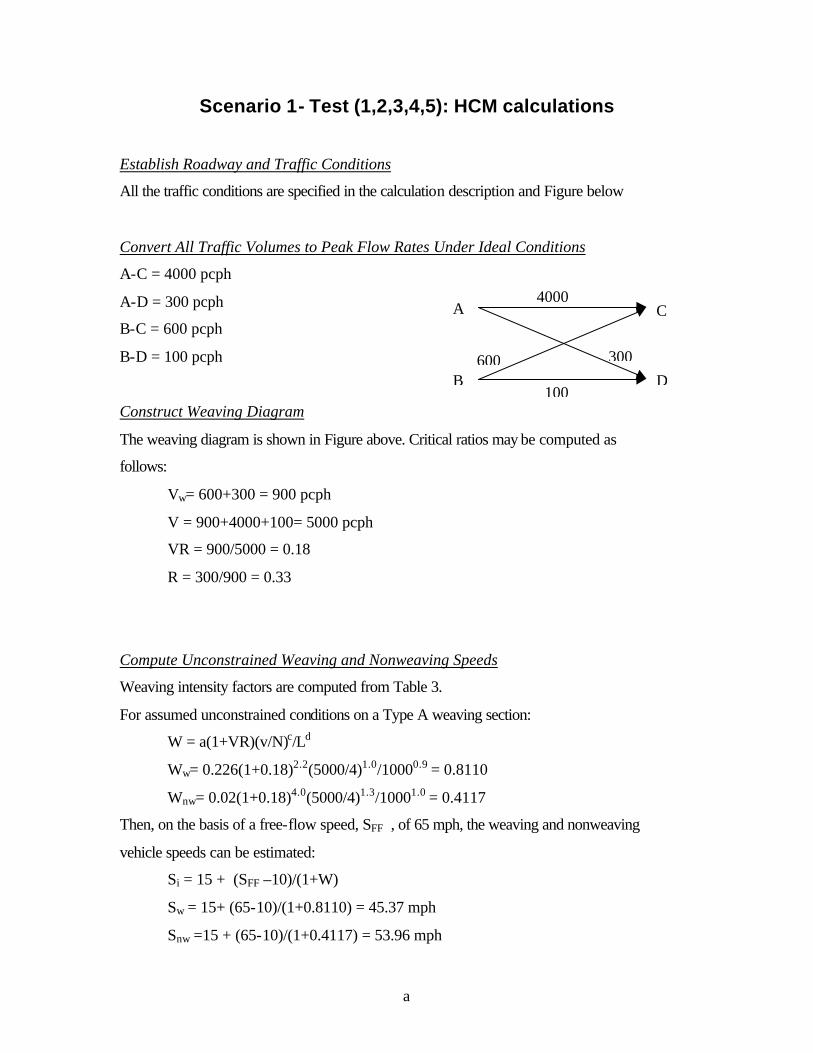
a
Scenario 1- Test (1,2,3,4,5): HCM calculations
Establish Roadway and Traffic Conditions
All the traffic conditions are specified in the calculation description and Figure below
Convert All Traffic Volumes to Peak Flow Rates Under Ideal Conditions
A-C = 4000 pcph
A-D = 300 pcph
B-C = 600 pcph
B-D = 100 pcph
Construct Weaving Diagram
The weaving diagram is shown in Figure above. Critical ratios may be computed as
follows:
Vw= 600+300 = 900 pcph
V = 900+4000+100= 5000 pcph
VR = 900/5000 = 0.18
R = 300/900 = 0.33
Compute Unconstrained Weaving and Nonweaving Speeds
Weaving intensity factors are computed from Table 3.
For assumed unconstrained conditions on a Type A weaving section:
W = a(1+VR)(v/N)c/Ld
Ww= 0.226(1+0.18)2.2(5000/4)1.0/10000.9 = 0.8110
Wnw= 0.02(1+0.18)4.0(5000/4)1.3/10001.0 = 0.4117
Then, on the basis of a free-flow speed, SFF , of 65 mph, the weaving and nonweaving
vehicle speeds can be estimated:
Si = 15 + (SFF –10)/(1+W)
Sw = 15+ (65-10)/(1+0.8110) = 45.37 mph
Snw =15 + (65-10)/(1+0.4117) = 53.96 mph
A
B
C
D 600 300
4000
100
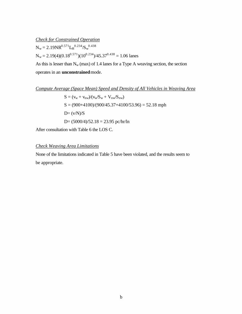
b
Check for Constrained Operation
Nw = 2.19NR0.571LH0.234/Sw
0.438
Nw = 2.19(4)(0.180.571)(100.234)/45.370.438 = 1.06 lanes
As this is lesser than Nw (max) of 1.4 lanes for a Type A weaving section, the section
operates in an unconstrained mode.
Compute Average (Space Mean) Speed and Density of All Vehicles in Weaving Area
S = (vw + vnw)/(vw/Sw + Vnw/Snw)
S = (900+4100)/(900/45.37+4100/53.96) = 52.18 mph
D= (v/N)/S
D= (5000/4)/52.18 = 23.95 pc/hr/ln
After consultation with Table 6 the LOS C.
Check Weaving Area Limitations
None of the limitations indicated in Table 5 have been violated, and the results seem to
be appropriate.
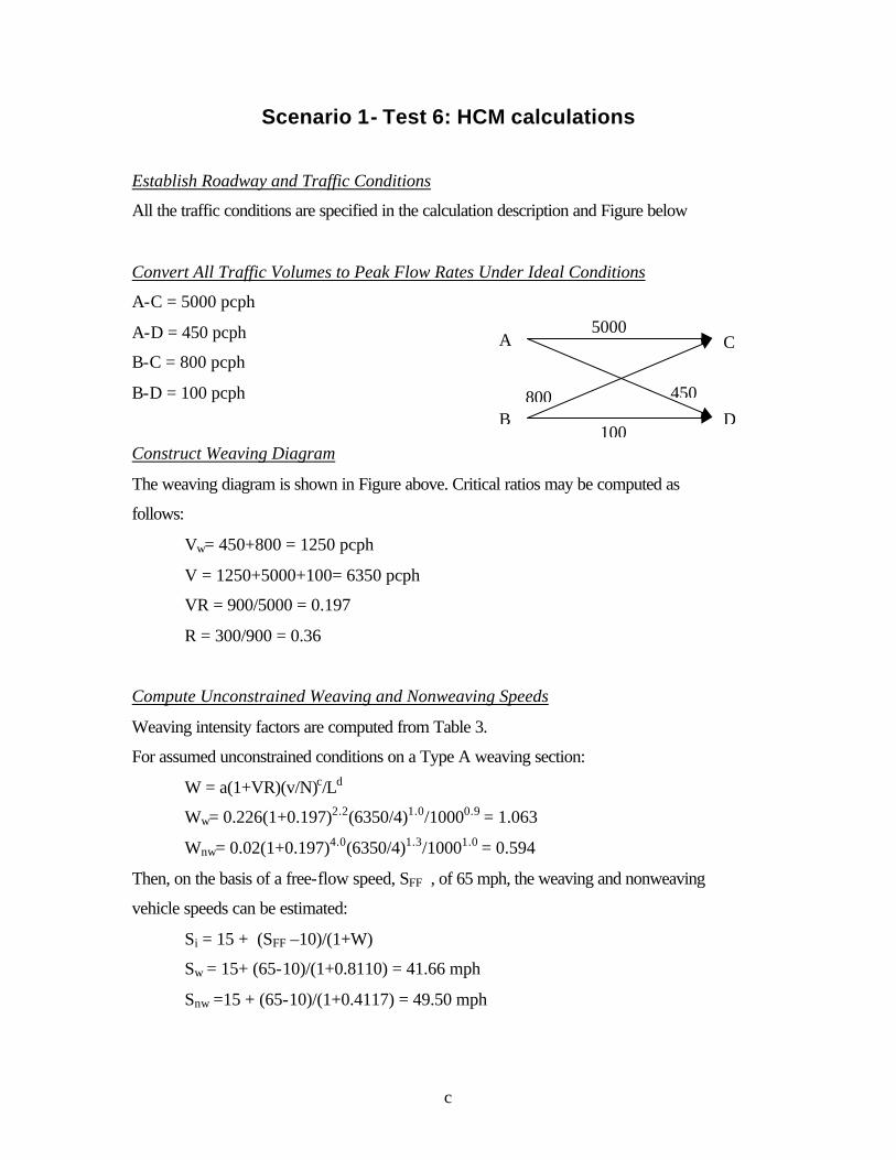
c
Scenario 1- Test 6: HCM calculations
Establish Roadway and Traffic Conditions
All the traffic conditions are specified in the calculation description and Figure below
Convert All Traffic Volumes to Peak Flow Rates Under Ideal Conditions
A-C = 5000 pcph
A-D = 450 pcph
B-C = 800 pcph
B-D = 100 pcph
Construct Weaving Diagram
The weaving diagram is shown in Figure above. Critical ratios may be computed as
follows:
Vw= 450+800 = 1250 pcph
V = 1250+5000+100= 6350 pcph
VR = 900/5000 = 0.197
R = 300/900 = 0.36
Compute Unconstrained Weaving and Nonweaving Speeds
Weaving intensity factors are computed from Table 3.
For assumed unconstrained conditions on a Type A weaving section:
W = a(1+VR)(v/N)c/Ld
Ww= 0.226(1+0.197)2.2(6350/4)1.0/10000.9 = 1.063
Wnw= 0.02(1+0.197)4.0(6350/4)1.3/10001.0 = 0.594
Then, on the basis of a free-flow speed, SFF , of 65 mph, the weaving and nonweaving
vehicle speeds can be estimated:
Si = 15 + (SFF –10)/(1+W)
Sw = 15+ (65-10)/(1+0.8110) = 41.66 mph
Snw =15 + (65-10)/(1+0.4117) = 49.50 mph
A
B
C
D 800 450
5000
100

d
Check for Constrained Operation
Nw = 2.19NR0.571LH0.234/Sw
0.438
Nw = 2.19(4)(0.1970.571)(100.234)/41.660.438 = 1.16 lanes
As this is lesser than Nw (max) of 1.4 lanes for a Type A weaving section, the section
operates in an unconstrained mode.
Compute Average (Space Mean) Speed and Density of All Vehicles in Weaving Area
S = (vw + vnw)/(vw/Sw + Vnw/Snw)
S = (1250+5100)/(1250/41.66+5100/49.50) = 47.73 mph
D= (v/N)/S
D= (6350/4)/47.73 = 33.26 pc/hr/ln
After consultation with Table 6 the LOS C.
Check Weaving Area Limitations
None of the limitations indicated in Table 5 have been violated, and the results seem to
be appropriate.

e
Scenario 1- Test 7: HCM calculations
Establish Roadway and Traffic Conditions
All the traffic conditions are specified in the calculation description and Figure below
Convert All Traffic Volumes to Peak Flow Rates Under Ideal Conditions
A-C = 6000 pcph
A-D = 600 pcph
B-C = 1000 pcph
B-D = 100 pcph
Construct Weaving Diagram
The weaving diagram is shown in Figure above. Critical ratios may be computed as
follows:
Vw= 1000+600 = 1600 pcph
V = 1600+6000+100= 7700 pcph
VR = 1600/7700 = 0.208
R = 600/1600 = 0.375
Compute Unconstrained Weaving and Nonweaving Speeds
Weaving intensity factors are computed from Table 3.
For assumed unconstrained conditions on a Type A weaving section:
W = a(1+VR)(v/N)c/Ld
Ww= 0.226(1+0.208)2.2(7700/4)1.0/10000.9 = 1.315
Wnw= 0.02(1+0.208)4.0(7700/4)1.3/10001.0 = 0.792
Then, on the basis of a free-flow speed, SFF , of 65 mph, the weaving and nonweaving
vehicle speeds can be estimated:
Si = 15 + (SFF –10)/(1+W)
Sw = 15+ (65-10)/(1+1.315) = 38.76 mph
Snw =15 + (65-10)/(1+0.792) = 45.69 mph
A
B
C
D 1000 600
6000
100
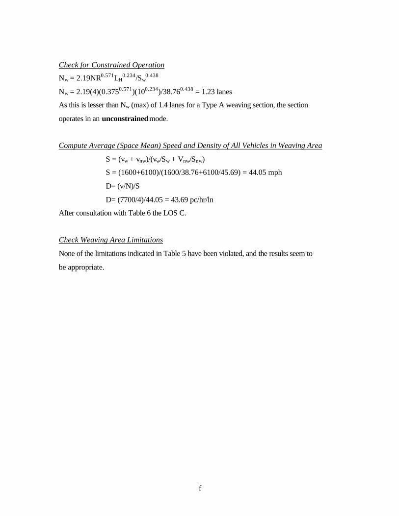
f
Check for Constrained Operation
Nw = 2.19NR0.571LH0.234/Sw
0.438
Nw = 2.19(4)(0.3750.571)(100.234)/38.760.438 = 1.23 lanes
As this is lesser than Nw (max) of 1.4 lanes for a Type A weaving section, the section
operates in an unconstrained mode.
Compute Average (Space Mean) Speed and Density of All Vehicles in Weaving Area
S = (vw + vnw)/(vw/Sw + Vnw/Snw)
S = (1600+6100)/(1600/38.76+6100/45.69) = 44.05 mph
D= (v/N)/S
D= (7700/4)/44.05 = 43.69 pc/hr/ln
After consultation with Table 6 the LOS C.
Check Weaving Area Limitations
None of the limitations indicated in Table 5 have been violated, and the results seem to
be appropriate.

g
Scenario 1- Test 8: HCM calculations
Establish Roadway and Traffic Conditions
All the traffic conditions are specified in the calculation description and Figure below
Convert All Traffic Volumes to Peak Flow Rates Under Ideal Conditions
A-C = 6000 pcph
A-D = 800 pcph
B-C = 1200 pcph
B-D = 100 pcph
Construct Weaving Diagram
The weaving diagram is shown in Figure above. Critical ratios may be computed as
follows:
Vw= 1200+800 = 2000 pcph
V = 2000+6000+100= 8100 pcph
VR = 2000/8100 = 0.247
R = 800/2000 = 0.4
Compute Unconstrained Weaving and Nonweaving Speeds
Weaving intensity factors are computed from Table 3.
For assumed unconstrained conditions on a Type A weaving section:
W = a(1+VR)(v/N)c/Ld
Ww= 0.226(1+0.247)2.2(8100/4)1.0/10000.9 = 1.484
Wnw= 0.02(1+0.247)4.0(8100/4)1.3/10001.0 = 0.961
Then, on the basis of a free-flow speed, SFF , of 65 mph, the weaving and nonweaving
vehicle speeds can be estimated:
Si = 15 + (SFF –10)/(1+W)
Sw = 15+ (65-10)/(1+1.484) = 37.14 mph
Snw =15 + (65-10)/(1+0.961) = 43.05 mph
A
B
C
D 1200 800
6000
100

h
Check for Constrained Operation
Nw = 2.19NR0.571LH0.234/Sw
0.438
Nw = 2.19(4)(0.40.571)(100.234)/37.140.438 = 1.386 lanes
As this is lesser than Nw (max) of 1.4 lanes for a Type A weaving section, the section
operates in an unconstrained mode.
Compute Average (Space Mean) Speed and Density of All Vehicles in Weaving Area
S = (vw + vnw)/(vw/Sw + Vnw/Snw)
S = (2000+6100)/(2000/37.14+6100/43.05) = 41.42 mph
D= (v/N)/S
D= (8100/4)/41.42 = 48.89 pc/hr/ln
After consultation with Table 6 the LOS C.
Check Weaving Area Limitations
None of the limitations indicated in Table 5 have been violated, and the results seem to
be appropriate.

i
Scenario 1- Test 9: HCM calculations
Establish Roadway and Traffic Conditions
All the traffic conditions are specified in the calculation description and Figure below
Convert All Traffic Volumes to Peak Flow Rates Under Ideal Conditions
A-C = 4500 pcph
A-D = 1200 pcph
B-C = 1800 pcph
B-D = 300 pcph
Construct Weaving Diagram
The weaving diagram is shown in Figure above. Critical ratios may be computed as
follows:
Vw= 1200+1800 = 3000 pcph
V = 3000+4500+300 = 7800 pcph
VR = 3000/7800 = 0.3846
R = 1200/3000 = 0.4
Compute Unconstrained Weaving and Nonweaving Speeds
Weaving intensity factors are computed from Table 3.
For assumed unconstrained conditions on a Type A weaving section:
W = a(1+VR)(v/N)c/Ld
Ww= 0.226(1+0.3846)2.2(7800/4)1.0/10000.9 = 1.7991
Wnw= 0.02(1+0.3846)4.0(7800/4)1.3/10001.0 = 1.3912
Then, on the basis of a free-flow speed, SFF , of 65 mph, the weaving and nonweaving
vehicle speeds can be estimated:
Si = 15 + (SFF –10)/(1+W)
Sw = 15+ (65-10)/(1+1.7991) = 34.65 mph
Snw =15 + (65-10)/(1+1.3912) = 38.00 mph
A
B
C
D 1800 1200
4500
300
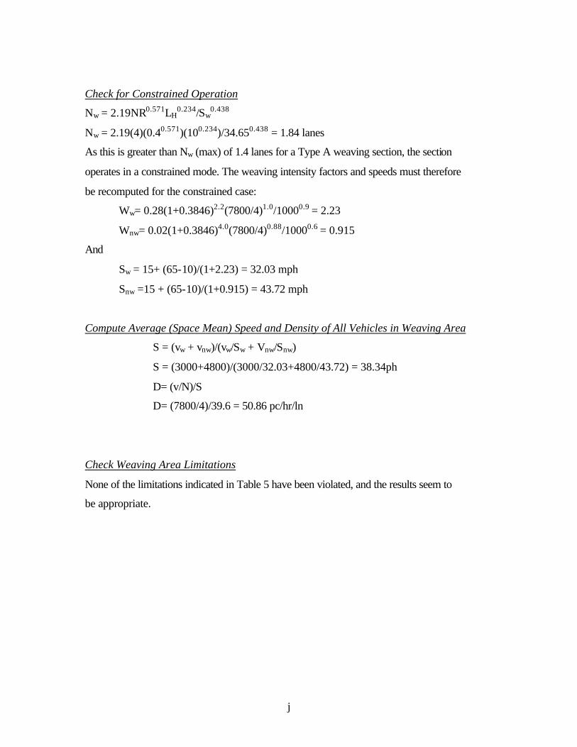
j
Check for Constrained Operation
Nw = 2.19NR0.571LH0.234/Sw
0.438
Nw = 2.19(4)(0.40.571)(100.234)/34.650.438 = 1.84 lanes
As this is greater than Nw (max) of 1.4 lanes for a Type A weaving section, the section
operates in a constrained mode. The weaving intensity factors and speeds must therefore
be recomputed for the constrained case:
Ww= 0.28(1+0.3846)2.2(7800/4)1.0/10000.9 = 2.23
Wnw= 0.02(1+0.3846)4.0(7800/4)0.88/10000.6 = 0.915
And
Sw = 15+ (65-10)/(1+2.23) = 32.03 mph
Snw =15 + (65-10)/(1+0.915) = 43.72 mph
Compute Average (Space Mean) Speed and Density of All Vehicles in Weaving Area
S = (vw + vnw)/(vw/Sw + Vnw/Snw)
S = (3000+4800)/(3000/32.03+4800/43.72) = 38.34ph
D= (v/N)/S
D= (7800/4)/39.6 = 50.86 pc/hr/ln
Check Weaving Area Limitations
None of the limitations indicated in Table 5 have been violated, and the results seem to
be appropriate.
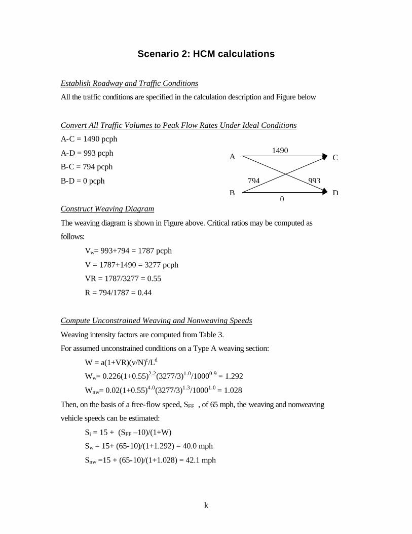
k
Scenario 2: HCM calculations
Establish Roadway and Traffic Conditions
All the traffic conditions are specified in the calculation description and Figure below
Convert All Traffic Volumes to Peak Flow Rates Under Ideal Conditions
A-C = 1490 pcph
A-D = 993 pcph
B-C = 794 pcph
B-D = 0 pcph
Construct Weaving Diagram
The weaving diagram is shown in Figure above. Critical ratios may be computed as
follows:
Vw= 993+794 = 1787 pcph
V = 1787+1490 = 3277 pcph
VR = 1787/3277 = 0.55
R = 794/1787 = 0.44
Compute Unconstrained Weaving and Nonweaving Speeds
Weaving intensity factors are computed from Table 3.
For assumed unconstrained conditions on a Type A weaving section:
W = a(1+VR)(v/N)c/Ld
Ww= 0.226(1+0.55)2.2(3277/3)1.0/10000.9 = 1.292
Wnw= 0.02(1+0.55)4.0(3277/3)1.3/10001.0 = 1.028
Then, on the basis of a free-flow speed, SFF , of 65 mph, the weaving and nonweaving
vehicle speeds can be estimated:
Si = 15 + (SFF –10)/(1+W)
Sw = 15+ (65-10)/(1+1.292) = 40.0 mph
Snw =15 + (65-10)/(1+1.028) = 42.1 mph
A
B
C
D 794 993
1490
0
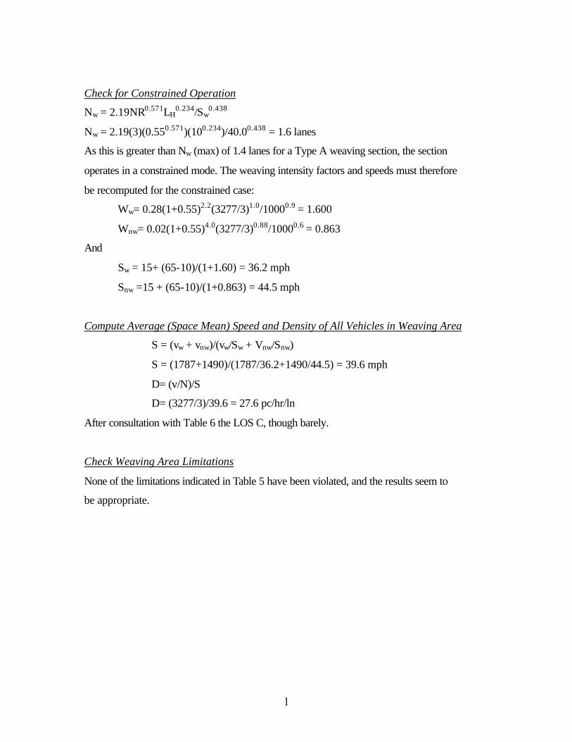
l
Check for Constrained Operation
Nw = 2.19NR0.571LH0.234/Sw
0.438
Nw = 2.19(3)(0.550.571)(100.234)/40.00.438 = 1.6 lanes
As this is greater than Nw (max) of 1.4 lanes for a Type A weaving section, the section
operates in a constrained mode. The weaving intensity factors and speeds must therefore
be recomputed for the constrained case:
Ww= 0.28(1+0.55)2.2(3277/3)1.0/10000.9 = 1.600
Wnw= 0.02(1+0.55)4.0(3277/3)0.88/10000.6 = 0.863
And
Sw = 15+ (65-10)/(1+1.60) = 36.2 mph
Snw =15 + (65-10)/(1+0.863) = 44.5 mph
Compute Average (Space Mean) Speed and Density of All Vehicles in Weaving Area
S = (vw + vnw)/(vw/Sw + Vnw/Snw)
S = (1787+1490)/(1787/36.2+1490/44.5) = 39.6 mph
D= (v/N)/S
D= (3277/3)/39.6 = 27.6 pc/hr/ln
After consultation with Table 6 the LOS C, though barely.
Check Weaving Area Limitations
None of the limitations indicated in Table 5 have been violated, and the results seem to
be appropriate.

m
APPENDIX-B
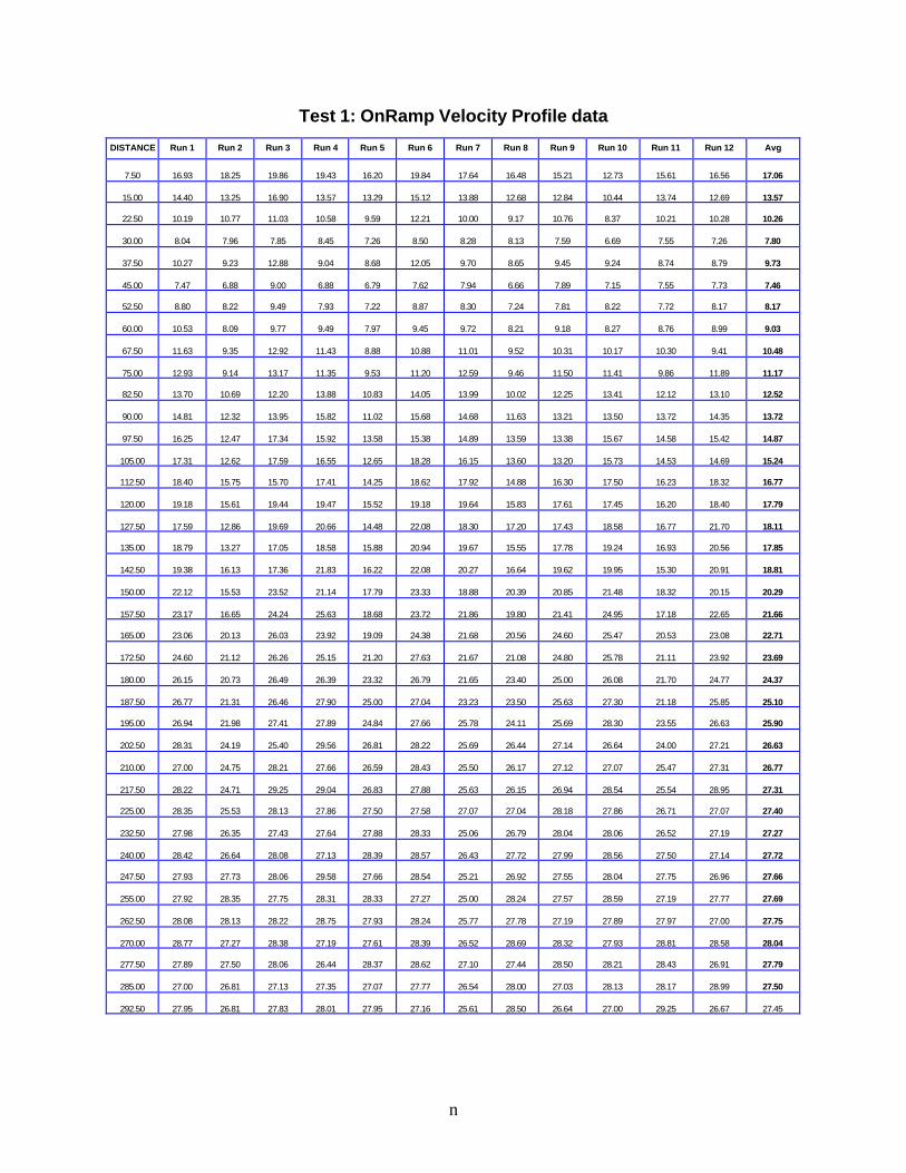
n
Test 1: OnRamp Velocity Profile data
DISTANCE Run 1 Run 2 Run 3 Run 4 Run 5 Run 6 Run 7 Run 8 Run 9 Run 10 Run 11 Run 12 Avg
7.50 16.93 18.25 19.86 19.43 16.20 19.84 17.64 16.48 15.21 12.73 15.61 16.56 17.06
15.00 14.40 13.25 16.90 13.57 13.29 15.12 13.88 12.68 12.84 10.44 13.74 12.69 13.57
22.50 10.19 10.77 11.03 10.58 9.59 12.21 10.00 9.17 10.76 8.37 10.21 10.28 10.26
30.00 8.04 7.96 7.85 8.45 7.26 8.50 8.28 8.13 7.59 6.69 7.55 7.26 7.80
37.50 10.27 9.23 12.88 9.04 8.68 12.05 9.70 8.65 9.45 9.24 8.74 8.79 9.73
45.00 7.47 6.88 9.00 6.88 6.79 7.62 7.94 6.66 7.89 7.15 7.55 7.73 7.46
52.50 8.80 8.22 9.49 7.93 7.22 8.87 8.30 7.24 7.81 8.22 7.72 8.17 8.17
60.00 10.53 8.09 9.77 9.49 7.97 9.45 9.72 8.21 9.18 8.27 8.76 8.99 9.03
67.50 11.63 9.35 12.92 11.43 8.88 10.88 11.01 9.52 10.31 10.17 10.30 9.41 10.48
75.00 12.93 9.14 13.17 11.35 9.53 11.20 12.59 9.46 11.50 11.41 9.86 11.89 11.17
82.50 13.70 10.69 12.20 13.88 10.83 14.05 13.99 10.02 12.25 13.41 12.12 13.10 12.52
90.00 14.81 12.32 13.95 15.82 11.02 15.68 14.68 11.63 13.21 13.50 13.72 14.35 13.72
97.50 16.25 12.47 17.34 15.92 13.58 15.38 14.89 13.59 13.38 15.67 14.58 15.42 14.87
105.00 17.31 12.62 17.59 16.55 12.65 18.28 16.15 13.60 13.20 15.73 14.53 14.69 15.24
112.50 18.40 15.75 15.70 17.41 14.25 18.62 17.92 14.88 16.30 17.50 16.23 18.32 16.77
120.00 19.18 15.61 19.44 19.47 15.52 19.18 19.64 15.83 17.61 17.45 16.20 18.40 17.79
127.50 17.59 12.86 19.69 20.66 14.48 22.08 18.30 17.20 17.43 18.58 16.77 21.70 18.11
135.00 18.79 13.27 17.05 18.58 15.88 20.94 19.67 15.55 17.78 19.24 16.93 20.56 17.85
142.50 19.38 16.13 17.36 21.83 16.22 22.08 20.27 16.64 19.62 19.95 15.30 20.91 18.81
150.00 22.12 15.53 23.52 21.14 17.79 23.33 18.88 20.39 20.85 21.48 18.32 20.15 20.29
157.50 23.17 16.65 24.24 25.63 18.68 23.72 21.86 19.80 21.41 24.95 17.18 22.65 21.66
165.00 23.06 20.13 26.03 23.92 19.09 24.38 21.68 20.56 24.60 25.47 20.53 23.08 22.71
172.50 24.60 21.12 26.26 25.15 21.20 27.63 21.67 21.08 24.80 25.78 21.11 23.92 23.69
180.00 26.15 20.73 26.49 26.39 23.32 26.79 21.65 23.40 25.00 26.08 21.70 24.77 24.37
187.50 26.77 21.31 26.46 27.90 25.00 27.04 23.23 23.50 25.63 27.30 21.18 25.85 25.10
195.00 26.94 21.98 27.41 27.89 24.84 27.66 25.78 24.11 25.69 28.30 23.55 26.63 25.90
202.50 28.31 24.19 25.40 29.56 26.81 28.22 25.69 26.44 27.14 26.64 24.00 27.21 26.63
210.00 27.00 24.75 28.21 27.66 26.59 28.43 25.50 26.17 27.12 27.07 25.47 27.31 26.77
217.50 28.22 24.71 29.25 29.04 26.83 27.88 25.63 26.15 26.94 28.54 25.54 28.95 27.31
225.00 28.35 25.53 28.13 27.86 27.50 27.58 27.07 27.04 28.18 27.86 26.71 27.07 27.40
232.50 27.98 26.35 27.43 27.64 27.88 28.33 25.06 26.79 28.04 28.06 26.52 27.19 27.27
240.00 28.42 26.64 28.08 27.13 28.39 28.57 26.43 27.72 27.99 28.56 27.50 27.14 27.72
247.50 27.93 27.73 28.06 29.58 27.66 28.54 25.21 26.92 27.55 28.04 27.75 26.96 27.66
255.00 27.92 28.35 27.75 28.31 28.33 27.27 25.00 28.24 27.57 28.59 27.19 27.77 27.69
262.50 28.08 28.13 28.22 28.75 27.93 28.24 25.77 27.78 27.19 27.89 27.97 27.00 27.75
270.00 28.77 27.27 28.38 27.19 27.61 28.39 26.52 28.69 28.32 27.93 28.81 28.58 28.04
277.50 27.89 27.50 28.06 26.44 28.37 28.62 27.10 27.44 28.50 28.21 28.43 26.91 27.79
285.00 27.00 26.81 27.13 27.35 27.07 27.77 26.54 28.00 27.03 28.13 28.17 28.99 27.50
292.50 27.95 26.81 27.83 28.01 27.95 27.16 25.61 28.50 26.64 27.00 29.25 26.67 27.45
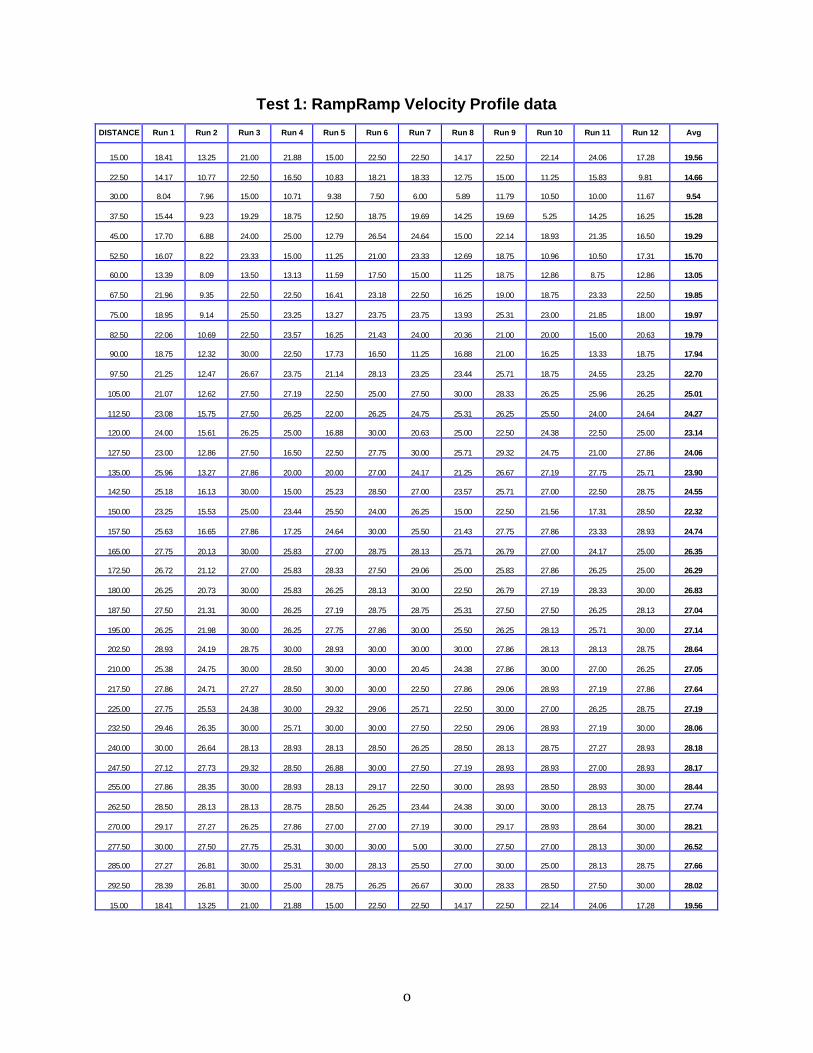
o
Test 1: RampRamp Velocity Profile data
DISTANCE Run 1 Run 2 Run 3 Run 4 Run 5 Run 6 Run 7 Run 8 Run 9 Run 10 Run 11 Run 12 Avg
15.00 18.41 13.25 21.00 21.88 15.00 22.50 22.50 14.17 22.50 22.14 24.06 17.28 19.56
22.50 14.17 10.77 22.50 16.50 10.83 18.21 18.33 12.75 15.00 11.25 15.83 9.81 14.66
30.00 8.04 7.96 15.00 10.71 9.38 7.50 6.00 5.89 11.79 10.50 10.00 11.67 9.54
37.50 15.44 9.23 19.29 18.75 12.50 18.75 19.69 14.25 19.69 5.25 14.25 16.25 15.28
45.00 17.70 6.88 24.00 25.00 12.79 26.54 24.64 15.00 22.14 18.93 21.35 16.50 19.29
52.50 16.07 8.22 23.33 15.00 11.25 21.00 23.33 12.69 18.75 10.96 10.50 17.31 15.70
60.00 13.39 8.09 13.50 13.13 11.59 17.50 15.00 11.25 18.75 12.86 8.75 12.86 13.05
67.50 21.96 9.35 22.50 22.50 16.41 23.18 22.50 16.25 19.00 18.75 23.33 22.50 19.85
75.00 18.95 9.14 25.50 23.25 13.27 23.75 23.75 13.93 25.31 23.00 21.85 18.00 19.97
82.50 22.06 10.69 22.50 23.57 16.25 21.43 24.00 20.36 21.00 20.00 15.00 20.63 19.79
90.00 18.75 12.32 30.00 22.50 17.73 16.50 11.25 16.88 21.00 16.25 13.33 18.75 17.94
97.50 21.25 12.47 26.67 23.75 21.14 28.13 23.25 23.44 25.71 18.75 24.55 23.25 22.70
105.00 21.07 12.62 27.50 27.19 22.50 25.00 27.50 30.00 28.33 26.25 25.96 26.25 25.01
112.50 23.08 15.75 27.50 26.25 22.00 26.25 24.75 25.31 26.25 25.50 24.00 24.64 24.27
120.00 24.00 15.61 26.25 25.00 16.88 30.00 20.63 25.00 22.50 24.38 22.50 25.00 23.14
127.50 23.00 12.86 27.50 16.50 22.50 27.75 30.00 25.71 29.32 24.75 21.00 27.86 24.06
135.00 25.96 13.27 27.86 20.00 20.00 27.00 24.17 21.25 26.67 27.19 27.75 25.71 23.90
142.50 25.18 16.13 30.00 15.00 25.23 28.50 27.00 23.57 25.71 27.00 22.50 28.75 24.55
150.00 23.25 15.53 25.00 23.44 25.50 24.00 26.25 15.00 22.50 21.56 17.31 28.50 22.32
157.50 25.63 16.65 27.86 17.25 24.64 30.00 25.50 21.43 27.75 27.86 23.33 28.93 24.74
165.00 27.75 20.13 30.00 25.83 27.00 28.75 28.13 25.71 26.79 27.00 24.17 25.00 26.35
172.50 26.72 21.12 27.00 25.83 28.33 27.50 29.06 25.00 25.83 27.86 26.25 25.00 26.29
180.00 26.25 20.73 30.00 25.83 26.25 28.13 30.00 22.50 26.79 27.19 28.33 30.00 26.83
187.50 27.50 21.31 30.00 26.25 27.19 28.75 28.75 25.31 27.50 27.50 26.25 28.13 27.04
195.00 26.25 21.98 30.00 26.25 27.75 27.86 30.00 25.50 26.25 28.13 25.71 30.00 27.14
202.50 28.93 24.19 28.75 30.00 28.93 30.00 30.00 30.00 27.86 28.13 28.13 28.75 28.64
210.00 25.38 24.75 30.00 28.50 30.00 30.00 20.45 24.38 27.86 30.00 27.00 26.25 27.05
217.50 27.86 24.71 27.27 28.50 30.00 30.00 22.50 27.86 29.06 28.93 27.19 27.86 27.64
225.00 27.75 25.53 24.38 30.00 29.32 29.06 25.71 22.50 30.00 27.00 26.25 28.75 27.19
232.50 29.46 26.35 30.00 25.71 30.00 30.00 27.50 22.50 29.06 28.93 27.19 30.00 28.06
240.00 30.00 26.64 28.13 28.93 28.13 28.50 26.25 28.50 28.13 28.75 27.27 28.93 28.18
247.50 27.12 27.73 29.32 28.50 26.88 30.00 27.50 27.19 28.93 28.93 27.00 28.93 28.17
255.00 27.86 28.35 30.00 28.93 28.13 29.17 22.50 30.00 28.93 28.50 28.93 30.00 28.44
262.50 28.50 28.13 28.13 28.75 28.50 26.25 23.44 24.38 30.00 30.00 28.13 28.75 27.74
270.00 29.17 27.27 26.25 27.86 27.00 27.00 27.19 30.00 29.17 28.93 28.64 30.00 28.21
277.50 30.00 27.50 27.75 25.31 30.00 30.00 5.00 30.00 27.50 27.00 28.13 30.00 26.52
285.00 27.27 26.81 30.00 25.31 30.00 28.13 25.50 27.00 30.00 25.00 28.13 28.75 27.66
292.50 28.39 26.81 30.00 25.00 28.75 26.25 26.67 30.00 28.33 28.50 27.50 30.00 28.02
15.00 18.41 13.25 21.00 21.88 15.00 22.50 22.50 14.17 22.50 22.14 24.06 17.28 19.56

p
Test 1: Through Velocity Profile data
DISTANCE Run 1 Run 2 Run 3 Run 4 Run 5 Run 6 Run 7 Run 8 Run 9 Run 10 Run 11 Run 12 Avg
7.50 13.79 9.15 18.05 12.26 7.71 12.48 13.64 9.77 9.21 11.57 14.42 10.81 11.90
15.00 15.22 10.79 18.38 13.45 8.00 14.50 14.38 10.47 10.64 12.49 14.84 12.08 12.94
22.50 14.43 11.75 18.33 13.71 10.32 15.91 15.60 11.55 11.92 13.96 14.46 12.76 13.73
30.00 15.02 11.22 18.03 14.13 10.48 16.40 15.52 11.84 11.68 13.65 13.97 12.25 13.68
37.50 14.79 12.04 16.51 15.15 11.35 16.53 15.91 12.17 12.42 14.75 15.10 12.46 14.10
45.00 17.58 14.57 18.98 17.44 14.11 18.17 16.57 12.77 13.76 16.56 16.49 14.88 15.99
52.50 18.27 15.31 20.61 18.74 14.52 19.69 18.57 14.74 14.61 17.36 17.27 15.67 17.11
60.00 18.67 16.12 20.47 19.53 15.03 20.19 19.44 15.34 15.30 18.35 17.69 16.45 17.71
67.50 20.18 16.81 21.44 20.77 15.72 20.13 20.12 16.58 16.86 20.03 18.73 17.54 18.74
75.00 21.70 19.55 22.12 22.57 18.90 22.03 20.68 18.04 18.82 21.79 20.49 20.12 20.57
82.50 22.51 19.22 22.96 22.87 19.00 23.22 21.64 19.13 19.06 21.76 21.27 21.24 21.16
90.00 22.44 20.48 23.23 23.73 19.26 23.96 22.26 19.62 20.38 22.41 22.31 21.76 21.82
97.50 23.70 21.01 23.34 24.75 20.50 24.78 23.05 20.67 21.71 23.25 21.94 22.85 22.63
105.00 24.72 21.98 24.77 24.97 21.85 24.76 24.34 21.09 23.02 25.02 23.47 23.88 23.66
112.50 24.44 21.20 25.07 24.98 21.80 25.90 25.15 22.52 22.72 25.14 23.19 24.79 23.91
120.00 25.40 21.77 25.77 25.94 22.57 25.52 25.08 23.37 24.14 25.13 23.97 25.69 24.53
127.50 25.15 23.24 25.79 26.20 23.80 25.32 25.60 24.04 24.72 25.87 24.06 25.53 24.94
135.00 26.06 24.73 26.28 26.64 24.68 25.90 26.09 24.65 25.61 25.78 24.75 26.22 25.62
142.50 25.91 24.62 27.05 26.47 25.11 26.30 25.75 25.53 25.39 26.17 25.40 26.61 25.86
150.00 26.37 24.99 26.73 27.61 25.43 27.05 25.59 25.34 26.39 27.38 24.69 27.03 26.22
157.50 26.75 25.06 27.07 27.25 26.07 26.98 25.81 26.28 26.85 27.13 25.92 27.50 26.56
165.00 27.18 25.90 27.44 27.77 26.54 27.60 25.21 25.93 26.82 27.58 25.44 28.06 26.79
172.50 27.21 26.33 27.55 27.70 26.90 27.84 25.84 26.02 26.73 27.52 25.85 27.90 26.95
180.00 27.24 26.77 27.66 28.11 27.25 27.91 26.47 26.12 26.65 27.47 26.26 27.74 27.14
187.50 27.65 27.17 27.51 27.96 26.92 27.79 27.06 26.63 26.81 27.80 26.88 27.83 27.33
195.00 28.15 27.37 27.62 28.28 27.42 27.92 26.45 27.52 27.58 27.74 26.42 28.03 27.54
202.50 28.13 26.92 27.69 27.50 26.99 28.06 27.27 27.68 27.33 27.77 27.05 27.76 27.51
210.00 28.18 27.61 27.93 28.23 27.05 27.99 26.83 27.49 27.79 27.88 26.81 28.00 27.65
217.50 28.33 27.96 27.53 28.01 27.68 28.05 26.68 27.63 27.52 27.91 27.42 28.05 27.73
225.00 28.13 27.50 27.78 27.73 27.10 28.08 27.35 27.21 27.65 28.15 27.70 28.18 27.71
232.50 27.93 27.78 27.78 28.29 27.31 28.05 27.65 27.95 27.65 27.58 27.28 28.04 27.78
240.00 28.13 27.82 28.07 27.68 27.45 27.92 27.37 27.61 27.66 28.04 27.79 28.00 27.80
247.50 27.91 27.77 28.09 28.26 27.66 27.44 27.62 27.73 28.02 28.03 27.62 27.87 27.83
255.00 28.03 28.18 28.34 28.53 27.67 28.18 27.42 27.77 27.56 27.89 27.80 28.05 27.95
262.50 27.99 28.35 28.07 27.96 27.32 27.76 27.30 27.92 27.88 27.96 28.15 27.68 27.86
270.00 27.85 27.79 27.84 27.72 27.80 28.04 27.06 27.44 28.37 27.85 28.11 27.39 27.77
277.50 28.15 27.77 28.06 27.77 27.64 27.97 27.51 27.76 28.02 28.23 28.32 28.00 27.93
285.00 27.73 28.10 28.13 27.60 27.41 27.79 27.19 27.78 28.02 27.91 28.03 27.73 27.78
292.50 27.80 27.50 28.00 27.73 27.25 28.03 27.15 27.61 27.67 28.04 27.90 27.90 27.72

q
Test 1: Offramp Velocity Profile data
DISTANCE Run 1 Run 2 Run 3 Run 4 Run 5 Run 6 Run 7 Run 8 Run 9 Run 10 Run 11 Run 12 Avg
7.50 11.84 8.18 16.41 13.79 7.87 13.83 16.07 8.31 9.25 10.82 14.25 8.68 11.61
15.00 13.78 7.60 16.10 12.94 7.50 16.15 14.62 10.04 10.46 9.75 11.75 10.56 11.77
22.50 12.03 8.87 14.67 10.63 7.57 9.89 11.77 9.41 6.93 11.55 13.91 9.67 10.57
30.00 9.28 8.13 10.52 8.71 6.92 8.98 9.66 8.06 7.14 9.89 11.01 8.01 8.86
37.50 7.95 7.65 8.47 9.15 5.77 9.43 8.08 5.93 7.58 8.67 8.80 7.41 7.91
45.00 7.75 6.70 7.00 7.17 6.72 7.93 8.20 7.68 7.59 5.60 7.38 7.23 7.25
52.50 8.11 7.41 9.51 7.50 7.59 7.95 7.29 7.40 8.28 8.80 8.06 7.15 7.92
60.00 8.71 8.51 9.34 10.50 8.28 9.18 8.90 8.63 8.85 9.52 8.86 8.38 8.97
67.50 10.41 9.07 11.67 9.57 8.86 10.53 12.45 8.51 10.16 9.55 9.71 9.12 9.97
75.00 10.68 9.47 11.79 11.59 9.83 12.63 10.67 9.43 10.00 11.09 8.69 7.92 10.32
82.50 10.38 12.39 14.53 13.59 10.90 13.90 11.25 11.18 9.40 12.00 10.77 10.16 11.70
90.00 13.54 11.88 16.42 15.54 12.03 13.79 15.19 12.00 11.91 17.06 13.27 12.05 13.72
97.50 14.13 12.23 15.78 13.46 11.18 17.58 15.47 11.72 12.86 12.95 15.00 15.75 14.01
105.00 17.50 14.82 17.28 14.74 14.84 19.69 15.24 12.68 15.63 17.68 14.32 17.41 15.99
112.50 18.13 15.21 21.39 16.07 14.09 22.50 16.63 15.77 15.91 19.20 16.94 19.29 17.59
120.00 19.17 17.14 19.85 19.35 16.35 22.86 22.03 16.07 18.52 24.46 19.63 20.83 19.69
127.50 19.39 19.14 22.06 15.75 16.62 23.30 22.92 18.75 16.10 20.63 19.58 20.83 19.59
135.00 19.90 16.92 22.14 17.41 17.96 23.75 22.20 16.54 17.77 25.10 16.43 20.11 19.69
142.50 21.89 13.50 25.63 18.87 15.91 25.66 18.17 16.40 18.09 25.76 18.64 24.38 20.24
150.00 21.03 18.75 26.25 20.81 17.95 23.93 22.50 19.69 21.82 26.07 19.62 25.94 22.03
157.50 23.37 21.47 25.42 19.89 22.50 27.61 21.48 20.36 20.74 27.08 15.39 24.83 22.51
165.00 25.07 22.00 25.83 21.79 24.29 24.20 22.17 21.39 25.56 27.07 19.89 23.18 23.54
172.50 25.93 23.39 27.38 24.11 24.38 26.57 20.77 24.25 26.43 26.95 24.52 24.94 24.97
180.00 26.57 24.78 28.44 26.43 25.31 28.93 21.92 25.00 25.00 26.83 23.57 26.70 25.79
187.50 27.43 25.45 26.84 25.00 28.39 27.60 24.17 26.70 25.94 26.54 22.03 28.98 26.26
195.00 27.16 25.50 29.42 26.79 27.39 28.24 26.25 25.65 26.74 28.88 21.20 27.69 26.74
202.50 27.42 27.27 28.13 28.44 27.27 28.75 25.91 25.91 25.94 29.25 23.75 28.42 27.20
210.00 28.06 26.88 28.37 27.19 27.95 27.66 26.43 26.70 28.30 29.42 25.31 28.50 27.56
217.50 28.42 27.39 29.50 28.24 28.66 28.27 20.45 26.70 27.41 28.85 23.21 29.21 27.19
225.00 28.71 27.61 28.13 27.32 27.81 28.00 20.10 26.25 29.06 28.13 23.57 29.38 27.01
232.50 27.92 27.86 28.50 27.98 29.12 28.68 25.80 24.75 28.56 28.03 26.07 28.93 27.68
240.00 28.80 28.75 28.64 28.57 27.67 27.92 25.66 27.90 28.88 29.64 27.69 28.19 28.19
247.50 29.21 27.30 29.38 27.92 27.59 29.66 25.13 28.75 28.97 27.08 28.24 28.50 28.14
255.00 28.78 27.75 29.12 28.13 28.42 28.03 24.08 28.36 27.79 27.98 27.86 27.00 27.77
262.50 30.00 27.38 28.25 28.25 28.24 28.50 26.93 28.13 29.06 28.00 29.50 28.42 28.39
270.00 28.01 28.70 28.75 29.50 28.75 28.42 23.70 27.78 28.88 27.81 29.42 29.44 28.26
277.50 29.09 28.44 27.00 29.21 28.89 28.64 22.92 28.37 29.22 27.66 28.82 28.59 28.07
285.00 28.85 28.04 27.08 26.67 27.75 29.12 20.83 29.22 27.07 28.56 28.93 27.50 27.47
292.50 27.36 29.46 29.40 29.38 27.63 27.92 24.64 27.14 28.13 27.19 28.93 28.24 27.95
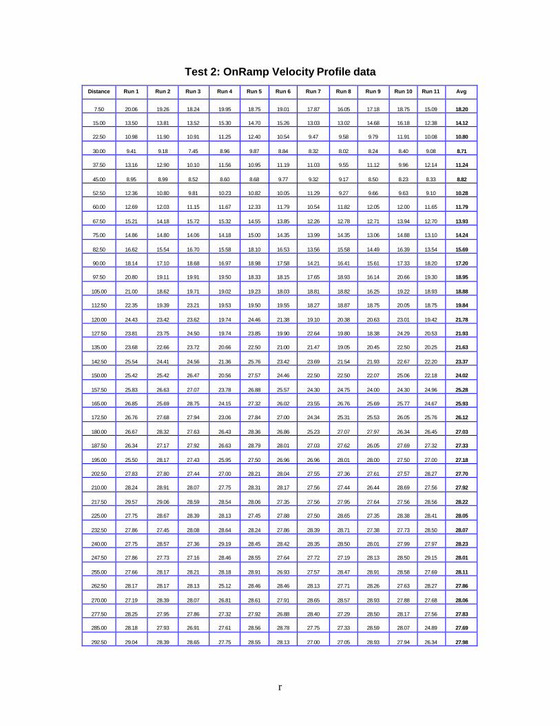
r
Test 2: OnRamp Velocity Profile data
Distance Run 1 Run 2 Run 3 Run 4 Run 5 Run 6 Run 7 Run 8 Run 9 Run 10 Run 11 Avg
7.50 20.06 19.26 18.24 19.95 18.75 19.01 17.87 16.05 17.18 18.75 15.09 18.20
15.00 13.50 13.81 13.52 15.30 14.70 15.26 13.03 13.02 14.68 16.18 12.38 14.12
22.50 10.98 11.90 10.91 11.25 12.40 10.54 9.47 9.58 9.79 11.91 10.08 10.80
30.00 9.41 9.18 7.45 8.96 9.87 8.84 8.32 8.02 8.24 8.40 9.08 8.71
37.50 13.16 12.90 10.10 11.56 10.95 11.19 11.03 9.55 11.12 9.96 12.14 11.24
45.00 8.95 8.99 8.52 8.60 8.68 9.77 9.32 9.17 8.50 8.23 8.33 8.82
52.50 12.36 10.80 9.81 10.23 10.82 10.05 11.29 9.27 9.66 9.63 9.10 10.28
60.00 12.69 12.03 11.15 11.67 12.33 11.79 10.54 11.82 12.05 12.00 11.65 11.79
67.50 15.21 14.18 15.72 15.32 14.55 13.85 12.26 12.78 12.71 13.94 12.70 13.93
75.00 14.86 14.80 14.06 14.18 15.00 14.35 13.99 14.35 13.06 14.88 13.10 14.24
82.50 16.62 15.54 16.70 15.58 18.10 16.53 13.56 15.58 14.49 16.39 13.54 15.69
90.00 18.14 17.10 18.68 16.97 18.98 17.58 14.21 16.41 15.61 17.33 18.20 17.20
97.50 20.80 19.11 19.91 19.50 18.33 18.15 17.65 18.93 16.14 20.66 19.30 18.95
105.00 21.00 18.62 19.71 19.02 19.23 18.03 18.81 18.82 16.25 19.22 18.93 18.88
112.50 22.35 19.39 23.21 19.53 19.50 19.55 18.27 18.87 18.75 20.05 18.75 19.84
120.00 24.43 23.42 23.62 19.74 24.46 21.38 19.10 20.38 20.63 23.01 19.42 21.78
127.50 23.81 23.75 24.50 19.74 23.85 19.90 22.64 19.80 18.38 24.29 20.53 21.93
135.00 23.68 22.66 23.72 20.66 22.50 21.00 21.47 19.05 20.45 22.50 20.25 21.63
142.50 25.54 24.41 24.56 21.36 25.76 23.42 23.69 21.54 21.93 22.67 22.20 23.37
150.00 25.42 25.42 26.47 20.56 27.57 24.46 22.50 22.50 22.07 25.06 22.18 24.02
157.50 25.83 26.63 27.07 23.78 26.88 25.57 24.30 24.75 24.00 24.30 24.96 25.28
165.00 26.85 25.69 28.75 24.15 27.32 26.02 23.55 26.76 25.69 25.77 24.67 25.93
172.50 26.76 27.68 27.94 23.06 27.84 27.00 24.34 25.31 25.53 26.05 25.76 26.12
180.00 26.67 28.32 27.63 26.43 28.36 26.86 25.23 27.07 27.97 26.34 26.45 27.03
187.50 26.34 27.17 27.92 26.63 28.79 28.01 27.03 27.62 26.05 27.69 27.32 27.33
195.00 25.50 28.17 27.43 25.95 27.50 26.96 26.96 28.01 28.00 27.50 27.00 27.18
202.50 27.83 27.80 27.44 27.00 28.21 28.04 27.55 27.36 27.61 27.57 28.27 27.70
210.00 28.24 28.91 28.07 27.75 28.31 28.17 27.56 27.44 26.44 28.69 27.56 27.92
217.50 29.57 29.06 28.59 28.54 28.06 27.35 27.56 27.95 27.64 27.56 28.56 28.22
225.00 27.75 28.67 28.39 28.13 27.45 27.88 27.50 28.65 27.35 28.38 28.41 28.05
232.50 27.86 27.45 28.08 28.64 28.24 27.86 28.39 28.71 27.38 27.73 28.50 28.07
240.00 27.75 28.57 27.36 29.19 28.45 28.42 28.35 28.50 28.01 27.99 27.97 28.23
247.50 27.86 27.73 27.16 28.46 28.55 27.64 27.72 27.19 28.13 28.50 29.15 28.01
255.00 27.66 28.17 28.21 28.18 28.91 26.93 27.57 28.47 28.91 28.58 27.69 28.11
262.50 28.17 28.17 28.13 25.12 28.46 28.46 28.13 27.71 28.26 27.63 28.27 27.86
270.00 27.19 28.39 28.07 26.81 28.61 27.91 28.65 28.57 28.93 27.88 27.68 28.06
277.50 28.25 27.95 27.86 27.32 27.92 26.88 28.40 27.29 28.50 28.17 27.56 27.83
285.00 28.18 27.93 26.91 27.61 28.56 28.78 27.75 27.33 28.59 28.07 24.89 27.69
292.50 29.04 28.39 28.65 27.75 28.55 28.13 27.00 27.05 28.93 27.94 26.34 27.98
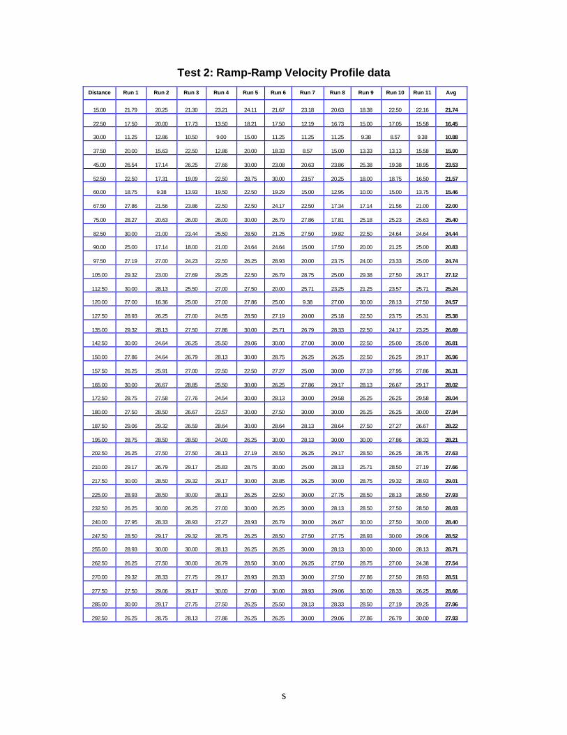
s
Test 2: Ramp-Ramp Velocity Profile data
Distance Run 1 Run 2 Run 3 Run 4 Run 5 Run 6 Run 7 Run 8 Run 9 Run 10 Run 11 Avg
15.00 21.79 20.25 21.30 23.21 24.11 21.67 23.18 20.63 18.38 22.50 22.16 21.74
22.50 17.50 20.00 17.73 13.50 18.21 17.50 12.19 16.73 15.00 17.05 15.58 16.45
30.00 11.25 12.86 10.50 9.00 15.00 11.25 11.25 11.25 9.38 8.57 9.38 10.88
37.50 20.00 15.63 22.50 12.86 20.00 18.33 8.57 15.00 13.33 13.13 15.58 15.90
45.00 26.54 17.14 26.25 27.66 30.00 23.08 20.63 23.86 25.38 19.38 18.95 23.53
52.50 22.50 17.31 19.09 22.50 28.75 30.00 23.57 20.25 18.00 18.75 16.50 21.57
60.00 18.75 9.38 13.93 19.50 22.50 19.29 15.00 12.95 10.00 15.00 13.75 15.46
67.50 27.86 21.56 23.86 22.50 22.50 24.17 22.50 17.34 17.14 21.56 21.00 22.00
75.00 28.27 20.63 26.00 26.00 30.00 26.79 27.86 17.81 25.18 25.23 25.63 25.40
82.50 30.00 21.00 23.44 25.50 28.50 21.25 27.50 19.82 22.50 24.64 24.64 24.44
90.00 25.00 17.14 18.00 21.00 24.64 24.64 15.00 17.50 20.00 21.25 25.00 20.83
97.50 27.19 27.00 24.23 22.50 26.25 28.93 20.00 23.75 24.00 23.33 25.00 24.74
105.00 29.32 23.00 27.69 29.25 22.50 26.79 28.75 25.00 29.38 27.50 29.17 27.12
112.50 30.00 28.13 25.50 27.00 27.50 20.00 25.71 23.25 21.25 23.57 25.71 25.24
120.00 27.00 16.36 25.00 27.00 27.86 25.00 9.38 27.00 30.00 28.13 27.50 24.57
127.50 28.93 26.25 27.00 24.55 28.50 27.19 20.00 25.18 22.50 23.75 25.31 25.38
135.00 29.32 28.13 27.50 27.86 30.00 25.71 26.79 28.33 22.50 24.17 23.25 26.69
142.50 30.00 24.64 26.25 25.50 29.06 30.00 27.00 30.00 22.50 25.00 25.00 26.81
150.00 27.86 24.64 26.79 28.13 30.00 28.75 26.25 26.25 22.50 26.25 29.17 26.96
157.50 26.25 25.91 27.00 22.50 22.50 27.27 25.00 30.00 27.19 27.95 27.86 26.31
165.00 30.00 26.67 28.85 25.50 30.00 26.25 27.86 29.17 28.13 26.67 29.17 28.02
172.50 28.75 27.58 27.76 24.54 30.00 28.13 30.00 29.58 26.25 26.25 29.58 28.04
180.00 27.50 28.50 26.67 23.57 30.00 27.50 30.00 30.00 26.25 26.25 30.00 27.84
187.50 29.06 29.32 26.59 28.64 30.00 28.64 28.13 28.64 27.50 27.27 26.67 28.22
195.00 28.75 28.50 28.50 24.00 26.25 30.00 28.13 30.00 30.00 27.86 28.33 28.21
202.50 26.25 27.50 27.50 28.13 27.19 28.50 26.25 29.17 28.50 26.25 28.75 27.63
210.00 29.17 26.79 29.17 25.83 28.75 30.00 25.00 28.13 25.71 28.50 27.19 27.66
217.50 30.00 28.50 29.32 29.17 30.00 28.85 26.25 30.00 28.75 29.32 28.93 29.01
225.00 28.93 28.50 30.00 28.13 26.25 22.50 30.00 27.75 28.50 28.13 28.50 27.93
232.50 26.25 30.00 26.25 27.00 30.00 26.25 30.00 28.13 28.50 27.50 28.50 28.03
240.00 27.95 28.33 28.93 27.27 28.93 26.79 30.00 26.67 30.00 27.50 30.00 28.40
247.50 28.50 29.17 29.32 28.75 26.25 28.50 27.50 27.75 28.93 30.00 29.06 28.52
255.00 28.93 30.00 30.00 28.13 26.25 26.25 30.00 28.13 30.00 30.00 28.13 28.71
262.50 26.25 27.50 30.00 26.79 28.50 30.00 26.25 27.50 28.75 27.00 24.38 27.54
270.00 29.32 28.33 27.75 29.17 28.93 28.33 30.00 27.50 27.86 27.50 28.93 28.51
277.50 27.50 29.06 29.17 30.00 27.00 30.00 28.93 29.06 30.00 28.33 26.25 28.66
285.00 30.00 29.17 27.75 27.50 26.25 25.50 28.13 28.33 28.50 27.19 29.25 27.96
292.50 26.25 28.75 28.13 27.86 26.25 26.25 30.00 29.06 27.86 26.79 30.00 27.93
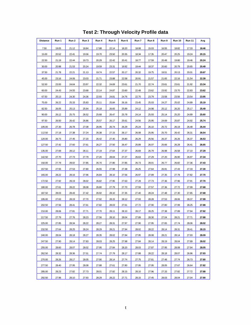
t
Test 2: Through Velocity Profile data
Distance Run 1 Run 2 Run 3 Run 4 Run 5 Run 6 Run 7 Run 8 Run 9 Run 10 Run 11 Avg
7.50 19.05 21.12 18.84 17.88 22.14 18.20 18.08 15.03 16.55 18.82 17.33 18.46
15.00 20.52 22.41 19.56 19.70 23.50 20.35 18.34 17.35 20.47 20.25 19.24 20.15
22.50 21.19 22.44 19.73 20.29 22.42 20.41 18.77 17.59 20.48 19.80 19.46 20.24
30.00 20.98 21.53 20.24 19.59 23.31 19.92 19.44 18.37 20.60 20.79 20.65 20.49
37.50 21.78 22.21 21.13 19.74 22.57 20.17 20.32 19.75 19.51 20.13 20.01 20.67
45.00 23.16 24.06 23.03 21.71 23.88 22.58 20.91 21.57 21.65 22.16 21.54 22.39
52.50 23.93 24.64 23.97 22.32 24.69 23.61 21.70 22.74 23.61 23.61 21.92 23.34
60.00 24.43 24.55 23.68 22.14 24.87 23.60 22.48 23.62 23.92 23.70 22.83 23.62
67.50 25.13 24.30 24.36 22.93 24.81 24.76 22.70 23.79 23.58 23.56 23.54 23.95
75.00 26.22 25.33 25.83 25.11 25.84 26.16 23.45 25.03 24.27 25.02 24.89 25.19
82.50 26.05 25.13 25.94 25.18 26.65 25.89 24.12 24.98 25.12 26.20 25.17 25.49
90.00 26.12 25.75 26.52 25.68 26.47 25.78 24.14 25.93 25.14 25.20 24.89 25.60
97.50 26.50 26.42 26.86 25.57 26.17 25.61 24.56 25.95 24.69 25.87 24.92 25.74
105.00 27.30 26.78 27.08 26.95 26.74 26.29 25.24 26.10 25.72 26.19 26.48 26.44
112.50 27.18 27.38 27.24 26.38 27.15 26.17 26.08 25.95 25.70 26.42 26.31 26.54
120.00 26.73 27.45 27.20 26.42 27.40 25.80 26.29 25.56 26.37 26.26 26.37 26.53
127.50 27.42 27.60 27.61 26.27 27.50 26.47 25.89 26.07 25.66 26.28 26.41 26.65
135.00 27.69 28.12 28.11 27.19 27.64 27.37 26.69 26.79 26.98 26.58 27.10 27.29
142.50 27.70 27.73 27.79 27.20 28.04 27.27 26.63 27.29 27.20 26.90 26.97 27.34
150.00 27.79 28.02 27.85 26.70 27.80 27.85 26.73 28.01 26.77 26.82 27.36 27.43
157.50 27.55 27.53 27.80 26.55 27.98 27.38 26.25 27.64 26.91 27.43 27.33 27.30
165.00 28.22 28.16 27.96 26.84 28.10 27.56 26.97 27.89 27.35 27.78 27.82 27.70
172.50 27.92 28.19 28.02 26.82 27.95 27.63 27.28 27.73 27.36 27.96 27.91 27.70
180.00 27.61 28.22 28.08 26.80 27.79 27.70 27.59 27.57 27.36 27.72 27.99 27.68
187.50 28.03 28.43 27.42 26.92 28.10 27.35 27.40 28.24 27.48 27.30 27.85 27.68
195.00 27.63 28.19 27.70 27.92 28.15 28.12 27.93 28.28 27.53 28.06 28.37 27.99
202.50 27.56 28.41 27.61 27.82 28.03 27.61 27.72 27.90 27.80 27.99 28.25 27.88
210.00 28.06 27.81 27.71 27.70 28.11 28.10 28.17 28.25 27.38 27.89 27.94 27.92
217.50 27.79 27.76 28.23 27.56 28.10 28.04 27.89 28.30 27.04 28.21 27.71 27.88
225.00 27.85 28.34 28.22 28.27 28.31 27.97 27.90 27.95 27.65 27.74 28.06 28.02
232.50 27.64 28.25 28.24 28.29 28.21 27.94 28.02 28.22 28.14 28.31 28.41 28.15
240.00 28.04 28.18 28.27 28.35 28.02 27.84 27.95 28.08 28.21 28.14 27.93 28.09
247.50 27.90 28.14 27.83 28.03 28.25 27.98 27.84 28.14 28.19 28.04 27.89 28.02
255.00 28.60 28.07 28.02 27.95 27.84 28.20 28.03 27.87 27.95 28.08 27.94 28.05
262.50 28.32 28.36 27.51 27.74 27.79 28.17 27.88 28.22 28.18 28.07 26.96 27.93
270.00 28.26 28.17 28.05 27.90 28.14 27.74 27.75 27.81 27.48 27.74 26.73 27.80
277.50 28.40 27.95 28.08 27.88 27.61 27.80 27.95 27.95 28.05 27.67 26.64 27.82
285.00 28.23 27.82 27.73 28.01 27.82 28.15 28.10 27.96 27.33 27.82 27.72 27.88
292.50 27.96 28.10 27.93 28.29 28.22 27.71 28.15 27.45 28.03 28.04 27.04 27.90

u
Test 2: Offramp Velocity Profile data
Distance Run 1 Run 2 Run 3 Run 4 Run 5 Run 6 Run 7 Run 8 Run 9 Run 10 Run 11 Avg
7.50 17.05 15.66 10.04 9.89 13.71 13.04 11.58 7.19 10.43 13.55 11.34 12.13
15.00 14.23 15.61 12.21 13.91 18.55 10.50 12.14 10.00 13.50 14.34 11.61 13.33
22.50 15.48 15.48 10.36 13.75 14.36 13.72 13.91 11.51 11.25 12.66 11.14 13.06
30.00 13.28 15.85 12.38 12.59 15.77 15.23 12.93 9.87 10.40 13.78 11.88 13.09
37.50 13.95 14.44 11.25 13.50 15.23 14.36 15.00 10.00 14.14 12.03 14.34 13.48
45.00 13.60 13.16 13.21 13.13 15.23 12.41 13.38 12.07 14.00 11.55 16.20 13.45
52.50 14.13 13.64 16.46 14.74 16.39 15.50 17.34 13.29 14.81 15.00 15.52 15.16
60.00 15.75 16.36 14.69 16.45 17.33 17.02 17.05 14.81 14.58 13.50 15.50 15.73
67.50 17.74 16.82 15.83 17.56 15.58 19.09 16.82 16.03 17.50 15.00 18.52 16.95
75.00 18.39 18.88 20.10 16.18 20.71 18.75 17.68 16.50 21.33 18.21 17.61 18.58
82.50 20.45 18.63 20.95 18.89 20.94 23.75 18.57 22.08 19.58 18.30 22.50 20.42
90.00 22.81 22.30 20.16 19.55 25.59 23.52 22.76 21.70 19.69 18.16 22.89 21.74
97.50 24.00 20.70 21.00 24.11 23.75 20.25 24.30 24.38 23.91 21.90 27.24 23.23
105.00 23.86 22.73 25.57 20.63 26.54 22.50 25.26 20.77 25.65 21.25 28.50 23.93
112.50 24.55 20.89 26.09 20.63 27.75 24.38 24.55 26.10 23.57 24.55 25.50 24.41
120.00 24.57 24.38 26.25 25.23 26.25 20.48 25.96 26.25 22.50 25.63 28.27 25.07
127.50 27.50 20.71 24.06 23.95 30.00 23.82 24.06 27.78 23.13 25.94 29.17 25.47
135.00 24.60 24.44 25.15 24.00 27.08 26.67 24.87 27.86 25.20 24.00 29.00 25.72
142.50 26.63 25.34 24.81 23.68 27.61 25.71 24.78 28.80 16.36 25.88 28.59 25.29
150.00 25.28 27.59 27.12 24.23 29.06 26.93 27.30 28.21 17.25 25.18 28.27 26.04
157.50 27.50 25.50 28.03 25.50 28.13 26.25 28.75 29.66 22.78 27.00 28.42 27.05
165.00 28.21 27.39 26.47 20.80 28.33 27.08 28.24 25.96 27.00 27.24 28.85 26.87
172.50 28.04 28.19 27.81 21.65 28.70 25.78 28.98 27.39 26.63 27.79 29.06 27.27
180.00 27.86 27.98 27.00 22.50 29.06 28.13 27.93 28.82 26.25 26.72 27.08 27.21
187.50 28.37 27.79 28.03 24.11 29.50 26.54 26.00 27.69 28.13 28.13 28.50 27.53
195.00 28.21 28.75 27.00 19.74 29.21 28.59 28.68 26.25 27.92 27.79 28.75 27.35
202.50 27.86 28.31 28.50 27.27 29.21 27.08 26.79 28.75 27.95 29.00 28.68 28.13
210.00 28.39 29.29 27.50 25.80 28.33 28.42 29.02 27.50 27.32 29.46 29.12 28.20
217.50 27.60 28.42 27.95 27.72 28.85 26.79 27.86 28.64 28.80 27.78 29.00 28.13
225.00 27.24 28.75 29.06 26.59 28.88 27.86 27.63 30.00 29.00 29.25 28.27 28.41
232.50 27.81 29.00 30.00 27.81 28.21 28.68 28.19 28.13 27.32 28.33 28.68 28.38
240.00 28.75 28.98 27.69 28.37 28.59 29.56 28.50 28.13 27.69 28.27 27.75 28.39
247.50 29.35 28.42 28.93 29.25 28.27 28.24 27.86 29.56 28.80 29.42 28.13 28.75
255.00 28.04 27.67 28.24 27.69 28.88 28.75 28.42 26.72 27.66 27.12 27.19 27.85
262.50 28.93 29.06 28.68 28.50 28.64 29.12 28.55 28.30 28.64 27.79 28.00 28.56
270.00 28.56 28.98 28.75 28.64 29.00 28.42 29.06 28.93 28.27 27.86 28.82 28.66
277.50 28.37 28.21 28.98 29.17 27.08 29.46 26.25 28.68 28.33 28.70 27.69 28.27
285.00 27.90 28.71 27.92 26.45 27.38 28.00 26.03 27.92 29.42 27.50 28.50 27.79
292.50 27.50 28.44 29.06 27.69 28.13 28.24 28.55 28.88 27.00 29.46 27.79 28.25
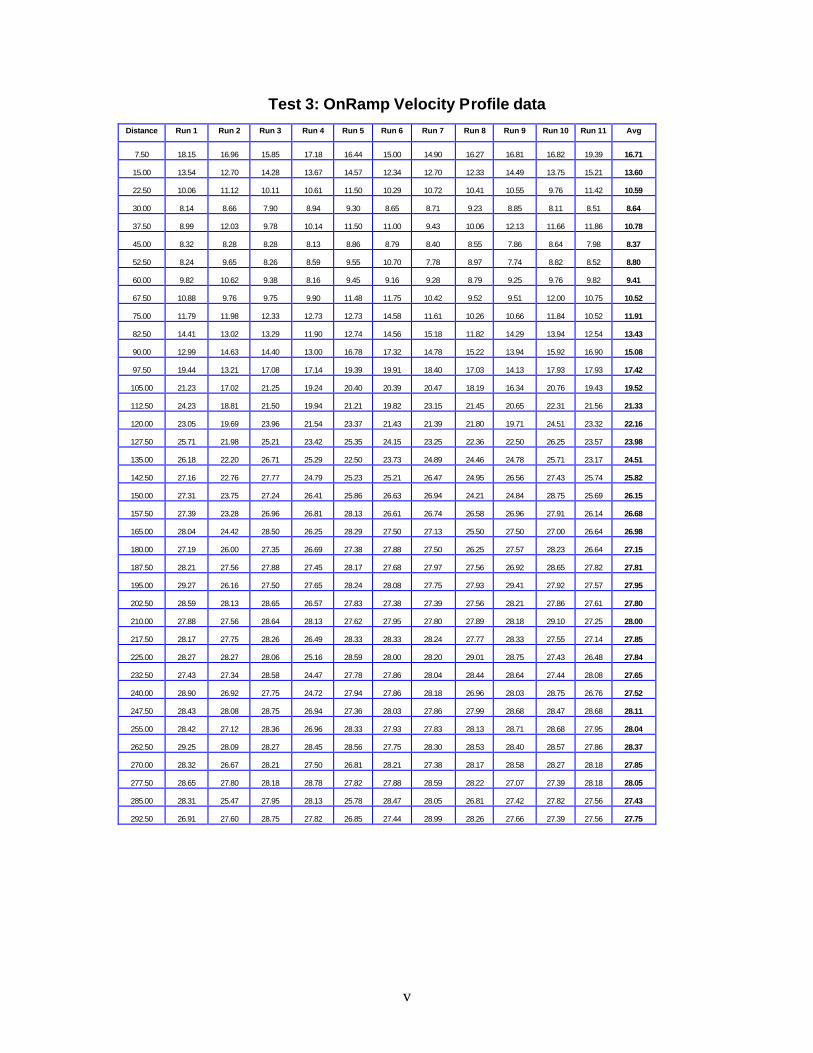
v
Test 3: OnRamp Velocity Profile data
Distance Run 1 Run 2 Run 3 Run 4 Run 5 Run 6 Run 7 Run 8 Run 9 Run 10 Run 11 Avg
7.50 18.15 16.96 15.85 17.18 16.44 15.00 14.90 16.27 16.81 16.82 19.39 16.71
15.00 13.54 12.70 14.28 13.67 14.57 12.34 12.70 12.33 14.49 13.75 15.21 13.60
22.50 10.06 11.12 10.11 10.61 11.50 10.29 10.72 10.41 10.55 9.76 11.42 10.59
30.00 8.14 8.66 7.90 8.94 9.30 8.65 8.71 9.23 8.85 8.11 8.51 8.64
37.50 8.99 12.03 9.78 10.14 11.50 11.00 9.43 10.06 12.13 11.66 11.86 10.78
45.00 8.32 8.28 8.28 8.13 8.86 8.79 8.40 8.55 7.86 8.64 7.98 8.37
52.50 8.24 9.65 8.26 8.59 9.55 10.70 7.78 8.97 7.74 8.82 8.52 8.80
60.00 9.82 10.62 9.38 8.16 9.45 9.16 9.28 8.79 9.25 9.76 9.82 9.41
67.50 10.88 9.76 9.75 9.90 11.48 11.75 10.42 9.52 9.51 12.00 10.75 10.52
75.00 11.79 11.98 12.33 12.73 12.73 14.58 11.61 10.26 10.66 11.84 10.52 11.91
82.50 14.41 13.02 13.29 11.90 12.74 14.56 15.18 11.82 14.29 13.94 12.54 13.43
90.00 12.99 14.63 14.40 13.00 16.78 17.32 14.78 15.22 13.94 15.92 16.90 15.08
97.50 19.44 13.21 17.08 17.14 19.39 19.91 18.40 17.03 14.13 17.93 17.93 17.42
105.00 21.23 17.02 21.25 19.24 20.40 20.39 20.47 18.19 16.34 20.76 19.43 19.52
112.50 24.23 18.81 21.50 19.94 21.21 19.82 23.15 21.45 20.65 22.31 21.56 21.33
120.00 23.05 19.69 23.96 21.54 23.37 21.43 21.39 21.80 19.71 24.51 23.32 22.16
127.50 25.71 21.98 25.21 23.42 25.35 24.15 23.25 22.36 22.50 26.25 23.57 23.98
135.00 26.18 22.20 26.71 25.29 22.50 23.73 24.89 24.46 24.78 25.71 23.17 24.51
142.50 27.16 22.76 27.77 24.79 25.23 25.21 26.47 24.95 26.56 27.43 25.74 25.82
150.00 27.31 23.75 27.24 26.41 25.86 26.63 26.94 24.21 24.84 28.75 25.69 26.15
157.50 27.39 23.28 26.96 26.81 28.13 26.61 26.74 26.58 26.96 27.91 26.14 26.68
165.00 28.04 24.42 28.50 26.25 28.29 27.50 27.13 25.50 27.50 27.00 26.64 26.98
180.00 27.19 26.00 27.35 26.69 27.38 27.88 27.50 26.25 27.57 28.23 26.64 27.15
187.50 28.21 27.56 27.88 27.45 28.17 27.68 27.97 27.56 26.92 28.65 27.82 27.81
195.00 29.27 26.16 27.50 27.65 28.24 28.08 27.75 27.93 29.41 27.92 27.57 27.95
202.50 28.59 28.13 28.65 26.57 27.83 27.38 27.39 27.56 28.21 27.86 27.61 27.80
210.00 27.88 27.56 28.64 28.13 27.62 27.95 27.80 27.89 28.18 29.10 27.25 28.00
217.50 28.17 27.75 28.26 26.49 28.33 28.33 28.24 27.77 28.33 27.55 27.14 27.85
225.00 28.27 28.27 28.06 25.16 28.59 28.00 28.20 29.01 28.75 27.43 26.48 27.84
232.50 27.43 27.34 28.58 24.47 27.78 27.86 28.04 28.44 28.64 27.44 28.08 27.65
240.00 28.90 26.92 27.75 24.72 27.94 27.86 28.18 26.96 28.03 28.75 26.76 27.52
247.50 28.43 28.08 28.75 26.94 27.36 28.03 27.86 27.99 28.68 28.47 28.68 28.11
255.00 28.42 27.12 28.36 26.96 28.33 27.93 27.83 28.13 28.71 28.68 27.95 28.04
262.50 29.25 28.09 28.27 28.45 28.56 27.75 28.30 28.53 28.40 28.57 27.86 28.37
270.00 28.32 26.67 28.21 27.50 26.81 28.21 27.38 28.17 28.58 28.27 28.18 27.85
277.50 28.65 27.80 28.18 28.78 27.82 27.88 28.59 28.22 27.07 27.39 28.18 28.05
285.00 28.31 25.47 27.95 28.13 25.78 28.47 28.05 26.81 27.42 27.82 27.56 27.43
292.50 26.91 27.60 28.75 27.82 26.85 27.44 28.99 28.26 27.66 27.39 27.56 27.75

w
Test 3: Ramp-Ramp Velocity Profile data
Distance Run 1 Run 2 Run 3 Run 4 Run 5 Run 6 Run 7 Run 8 Run 9 Run 10 Run 11 Avg
15.00 20.36 23.86 17.10 18.75 21.82 22.14 16.43 18.26 19.69 19.38 18.90 19.70
22.50 15.58 10.83 9.00 17.50 22.50 15.00 10.31 15.00 17.50 15.00 15.00 14.84
30.00 6.56 11.25 8.08 10.50 15.00 12.50 9.00 7.03 15.00 11.25 5.63 10.16
37.50 15.54 13.13 13.93 16.88 22.50 22.50 16.73 8.25 17.88 19.29 16.88 16.68
45.00 26.25 28.50 16.88 21.00 21.00 28.27 16.50 16.88 17.34 20.77 24.11 21.59
52.50 18.00 20.63 15.00 12.00 17.50 18.75 21.00 18.75 9.17 9.38 12.86 15.73
60.00 17.81 15.00 11.25 16.50 11.25 15.00 17.50 11.25 10.83 11.67 12.27 13.67
67.50 23.18 20.83 21.14 16.88 25.50 20.00 22.50 13.13 15.00 18.13 15.44 19.25
75.00 26.25 23.50 20.00 22.50 26.67 25.83 23.57 25.91 21.14 23.18 12.08 22.78
82.50 20.25 20.63 21.25 15.00 26.25 24.64 22.50 18.46 10.71 15.00 18.13 19.35
90.00 22.50 24.38 20.83 15.00 18.75 16.88 26.25 17.14 17.14 19.29 17.25 19.58
97.50 23.75 25.00 23.33 25.00 27.00 26.79 24.64 15.00 23.44 23.75 19.77 23.41
105.00 27.27 26.88 25.00 27.27 30.00 28.13 27.50 25.00 20.77 24.64 16.67 25.37
112.50 25.50 18.75 25.00 22.50 27.50 27.86 27.50 21.43 18.75 18.75 22.50 23.28
120.00 30.00 25.00 25.23 30.00 30.00 24.38 26.25 15.00 25.50 23.33 22.50 25.20
127.50 27.19 28.33 25.00 25.23 27.86 26.25 28.75 20.63 25.50 28.13 21.56 25.86
135.00 27.12 27.95 25.00 28.93 28.50 26.25 27.50 20.50 27.86 27.50 17.50 25.87
142.50 28.75 22.50 24.64 26.25 30.00 28.75 25.00 18.75 22.50 26.25 24.75 25.29
150.00 28.75 27.00 27.50 22.50 25.00 25.71 30.00 21.56 27.50 27.75 25.83 26.28
157.50 28.33 27.27 22.50 28.64 28.75 30.00 28.13 24.38 27.27 27.86 26.25 27.22
165.00 30.00 30.00 28.50 28.75 30.00 28.50 30.00 29.17 25.71 30.00 25.83 28.77
172.50 28.59 27.50 28.42 26.88 27.50 30.00 29.38 29.05 27.50 29.63 27.19 28.33
180.00 27.19 27.50 28.33 25.00 27.50 28.33 28.75 28.93 24.38 29.25 24.75 27.26
187.50 27.50 29.25 25.00 29.25 30.00 28.50 29.06 27.19 29.25 30.00 28.13 28.47
195.00 30.00 28.93 25.00 28.75 28.50 28.50 28.13 29.17 28.75 27.50 28.93 28.38
202.50 28.33 27.50 28.50 26.25 27.50 30.00 27.00 27.50 25.50 25.00 26.25 27.21
210.00 28.13 30.00 28.93 25.50 26.25 30.00 28.50 28.13 30.00 27.75 25.50 28.06
217.50 28.33 29.32 25.50 28.33 27.00 27.86 30.00 28.93 28.75 28.75 27.00 28.16
225.00 28.93 28.93 28.13 30.00 28.13 28.13 30.00 30.00 27.50 28.50 26.25 28.59
232.50 29.17 27.50 30.00 30.00 27.50 27.00 28.75 27.00 30.00 24.64 28.75 28.21
240.00 30.00 26.79 30.00 26.67 28.13 29.06 28.50 27.00 24.38 27.19 28.13 27.80
247.50 29.25 28.50 30.00 27.86 30.00 30.00 28.75 27.00 30.00 26.25 28.50 28.74
255.00 26.59 28.75 27.50 26.25 30.00 27.50 28.13 30.00 30.00 30.00 28.33 28.46
262.50 27.50 27.50 29.06 22.50 28.13 28.13 27.86 27.86 30.00 29.06 28.75 27.85
270.00 26.67 27.50 28.93 29.06 28.13 28.33 30.00 30.00 28.50 29.06 27.50 28.52
277.50 28.13 28.33 27.50 26.67 27.00 27.50 28.93 27.86 28.50 28.75 28.50 27.97
285.00 28.64 28.50 30.00 30.00 26.25 28.50 27.00 30.00 28.50 24.38 27.95 28.16
292.50 25.83 27.50 30.00 22.50 27.50 28.13 28.75 30.00 27.50 30.00 28.64 27.85
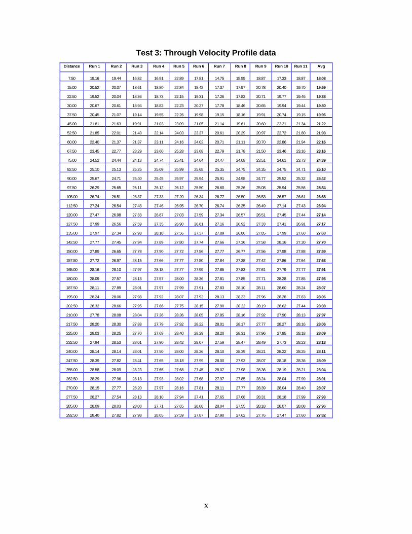
x
Test 3: Through Velocity Profile data
Distance Run 1 Run 2 Run 3 Run 4 Run 5 Run 6 Run 7 Run 8 Run 9 Run 10 Run 11 Avg
7.50 19.16 19.44 16.82 16.91 22.89 17.81 14.75 15.99 18.87 17.33 18.87 18.08
15.00 20.52 20.07 18.61 18.80 22.84 18.42 17.37 17.97 20.78 20.40 19.70 19.59
22.50 19.52 20.04 18.36 18.73 22.15 19.31 17.26 17.82 20.71 19.77 19.46 19.38
30.00 20.67 20.61 18.94 18.82 22.23 20.27 17.78 18.46 20.65 19.94 19.44 19.80
37.50 20.45 21.07 19.14 19.55 22.26 19.98 19.15 18.16 19.91 20.74 19.15 19.96
45.00 21.81 21.63 19.91 21.03 23.09 21.05 21.14 19.61 20.60 22.21 21.34 21.22
52.50 21.85 22.01 21.43 22.14 24.03 23.37 20.61 20.29 20.97 22.72 21.80 21.93
60.00 22.40 21.37 21.37 23.11 24.16 24.02 20.71 21.11 20.70 22.86 21.94 22.16
67.50 23.45 22.77 23.29 23.60 25.28 23.68 22.79 21.78 21.50 23.46 23.16 23.16
75.00 24.52 24.44 24.13 24.74 25.41 24.64 24.47 24.08 23.51 24.61 23.73 24.39
82.50 25.10 25.13 25.25 25.09 25.99 25.68 25.35 24.75 24.35 24.75 24.71 25.10
90.00 25.67 24.71 25.40 25.45 25.97 25.94 25.91 24.98 24.77 25.52 25.32 25.42
97.50 26.29 25.65 26.11 26.12 26.12 25.50 26.60 25.26 25.08 25.94 25.56 25.84
105.00 26.74 26.51 26.37 27.33 27.20 26.34 26.77 26.50 26.53 26.57 26.61 26.68
112.50 27.24 26.54 27.43 27.46 26.95 26.70 26.74 26.25 26.49 27.14 27.43 26.94
120.00 27.47 26.98 27.33 26.87 27.03 27.59 27.34 26.57 26.51 27.45 27.44 27.14
127.50 27.99 26.56 27.59 27.35 26.90 26.81 27.16 26.92 27.33 27.41 26.91 27.17
135.00 27.97 27.34 27.98 28.10 27.56 27.37 27.89 26.86 27.85 27.99 27.60 27.68
142.50 27.77 27.45 27.94 27.89 27.80 27.74 27.66 27.36 27.58 28.16 27.30 27.70
150.00 27.89 26.65 27.78 27.90 27.72 27.56 27.77 26.77 27.56 27.98 27.88 27.59
157.50 27.72 26.97 28.15 27.66 27.77 27.50 27.84 27.38 27.42 27.86 27.64 27.63
165.00 28.16 28.10 27.97 28.18 27.77 27.99 27.85 27.83 27.61 27.79 27.77 27.91
180.00 28.09 27.57 28.13 27.57 28.00 28.36 27.81 27.85 27.71 28.28 27.85 27.93
187.50 28.11 27.89 28.01 27.97 27.99 27.91 27.83 28.10 28.11 28.60 28.24 28.07
195.00 28.24 28.06 27.98 27.92 28.07 27.92 28.13 28.23 27.96 28.28 27.83 28.06
202.50 28.32 28.66 27.95 27.66 27.75 28.15 27.90 28.22 28.19 28.62 27.44 28.08
210.00 27.78 28.08 28.04 27.36 28.36 28.05 27.85 28.16 27.92 27.90 28.13 27.97
217.50 28.20 28.30 27.88 27.79 27.92 28.22 28.01 28.17 27.77 28.27 28.16 28.06
225.00 28.03 28.25 27.70 27.69 28.40 28.29 28.20 28.31 27.96 27.95 28.18 28.09
232.50 27.94 28.53 28.01 27.90 28.42 28.07 27.59 28.47 28.49 27.73 28.23 28.13
240.00 28.14 28.14 28.01 27.50 28.00 28.26 28.10 28.39 28.21 28.22 28.25 28.11
247.50 28.39 27.82 28.41 27.65 28.18 27.99 28.00 27.93 28.07 28.18 28.36 28.09
255.00 28.58 28.09 28.23 27.65 27.68 27.45 28.07 27.98 28.36 28.19 28.21 28.04
262.50 28.29 27.96 28.13 27.93 28.02 27.68 27.97 27.85 28.24 28.04 27.99 28.01
270.00 28.15 27.77 28.20 27.97 28.16 27.81 28.11 27.77 28.39 28.04 28.40 28.07
277.50 28.27 27.54 28.13 28.10 27.94 27.41 27.65 27.68 28.31 28.18 27.99 27.93
285.00 28.09 28.03 28.08 27.71 27.65 28.08 28.04 27.55 28.18 28.07 28.08 27.96
292.50 28.40 27.82 27.98 28.05 27.59 27.87 27.90 27.62 27.76 27.47 27.60 27.82
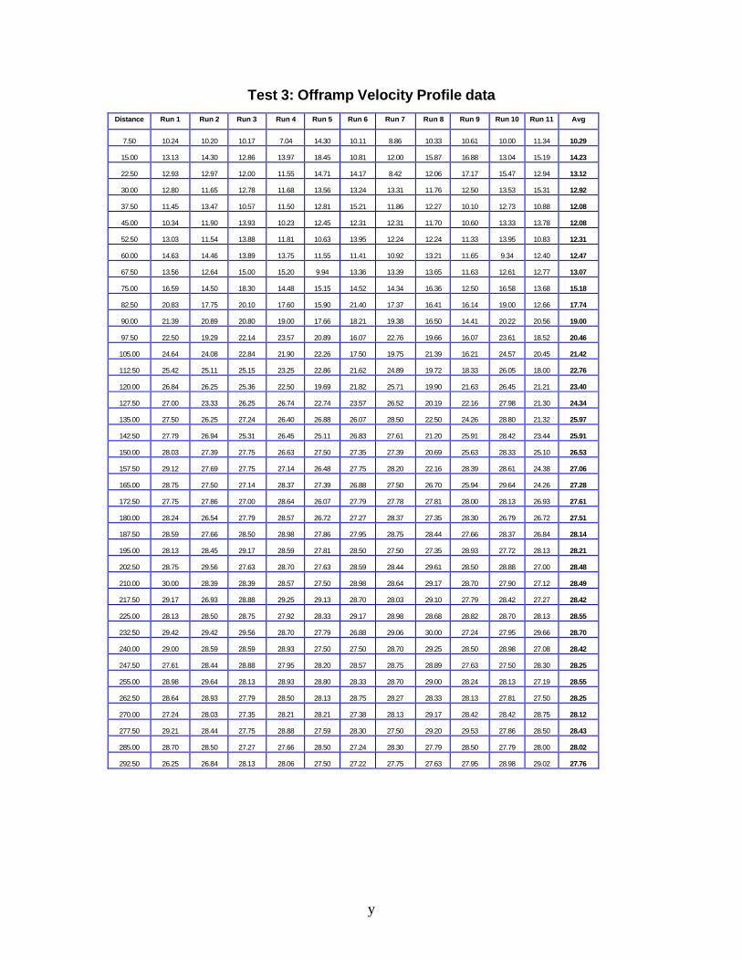
y
Test 3: Offramp Velocity Profile data
Distance Run 1 Run 2 Run 3 Run 4 Run 5 Run 6 Run 7 Run 8 Run 9 Run 10 Run 11 Avg
7.50 10.24 10.20 10.17 7.04 14.30 10.11 8.86 10.33 10.61 10.00 11.34 10.29
15.00 13.13 14.30 12.86 13.97 18.45 10.81 12.00 15.87 16.88 13.04 15.19 14.23
22.50 12.93 12.97 12.00 11.55 14.71 14.17 8.42 12.06 17.17 15.47 12.94 13.12
30.00 12.80 11.65 12.78 11.68 13.56 13.24 13.31 11.76 12.50 13.53 15.31 12.92
37.50 11.45 13.47 10.57 11.50 12.81 15.21 11.86 12.27 10.10 12.73 10.88 12.08
45.00 10.34 11.90 13.93 10.23 12.45 12.31 12.31 11.70 10.60 13.33 13.78 12.08
52.50 13.03 11.54 13.88 11.81 10.63 13.95 12.24 12.24 11.33 13.95 10.83 12.31
60.00 14.63 14.46 13.89 13.75 11.55 11.41 10.92 13.21 11.65 9.34 12.40 12.47
67.50 13.56 12.64 15.00 15.20 9.94 13.36 13.39 13.65 11.63 12.61 12.77 13.07
75.00 16.59 14.50 18.30 14.48 15.15 14.52 14.34 16.36 12.50 16.58 13.68 15.18
82.50 20.83 17.75 20.10 17.60 15.90 21.40 17.37 16.41 16.14 19.00 12.66 17.74
90.00 21.39 20.89 20.80 19.00 17.66 18.21 19.38 16.50 14.41 20.22 20.56 19.00
97.50 22.50 19.29 22.14 23.57 20.89 16.07 22.76 19.66 16.07 23.61 18.52 20.46
105.00 24.64 24.08 22.84 21.90 22.26 17.50 19.75 21.39 16.21 24.57 20.45 21.42
112.50 25.42 25.11 25.15 23.25 22.86 21.62 24.89 19.72 18.33 26.05 18.00 22.76
120.00 26.84 26.25 25.36 22.50 19.69 21.82 25.71 19.90 21.63 26.45 21.21 23.40
127.50 27.00 23.33 26.25 26.74 22.74 23.57 26.52 20.19 22.16 27.98 21.30 24.34
135.00 27.50 26.25 27.24 26.40 26.88 26.07 28.50 22.50 24.26 28.80 21.32 25.97
142.50 27.79 26.94 25.31 26.45 25.11 26.83 27.61 21.20 25.91 28.42 23.44 25.91
150.00 28.03 27.39 27.75 26.63 27.50 27.35 27.39 20.69 25.63 28.33 25.10 26.53
157.50 29.12 27.69 27.75 27.14 26.48 27.75 28.20 22.16 28.39 28.61 24.38 27.06
165.00 28.75 27.50 27.14 28.37 27.39 26.88 27.50 26.70 25.94 29.64 24.26 27.28
172.50 27.75 27.86 27.00 28.64 26.07 27.79 27.78 27.81 28.00 28.13 26.93 27.61
180.00 28.24 26.54 27.79 28.57 26.72 27.27 28.37 27.35 28.30 26.79 26.72 27.51
187.50 28.59 27.66 28.50 28.98 27.86 27.95 28.75 28.44 27.66 28.37 26.84 28.14
195.00 28.13 28.45 29.17 28.59 27.81 28.50 27.50 27.35 28.93 27.72 28.13 28.21
202.50 28.75 29.56 27.63 28.70 27.63 28.59 28.44 29.61 28.50 28.88 27.00 28.48
210.00 30.00 28.39 28.39 28.57 27.50 28.98 28.64 29.17 28.70 27.90 27.12 28.49
217.50 29.17 26.93 28.88 29.25 29.13 28.70 28.03 29.10 27.79 28.42 27.27 28.42
225.00 28.13 28.50 28.75 27.92 28.33 29.17 28.98 28.68 28.82 28.70 28.13 28.55
232.50 29.42 29.42 29.56 28.70 27.79 26.88 29.06 30.00 27.24 27.95 29.66 28.70
240.00 29.00 28.59 28.59 28.93 27.50 27.50 28.70 29.25 28.50 28.98 27.08 28.42
247.50 27.61 28.44 28.88 27.95 28.20 28.57 28.75 28.89 27.63 27.50 28.30 28.25
255.00 28.98 29.64 28.13 28.93 28.80 28.33 28.70 29.00 28.24 28.13 27.19 28.55
262.50 28.64 28.93 27.79 28.50 28.13 28.75 28.27 28.33 28.13 27.81 27.50 28.25
270.00 27.24 28.03 27.35 28.21 28.21 27.38 28.13 29.17 28.42 28.42 28.75 28.12
277.50 29.21 28.44 27.75 28.88 27.59 28.30 27.50 29.20 29.53 27.86 28.50 28.43
285.00 28.70 28.50 27.27 27.66 28.50 27.24 28.30 27.79 28.50 27.79 28.00 28.02
292.50 26.25 26.84 28.13 28.06 27.50 27.22 27.75 27.63 27.95 28.98 29.02 27.76
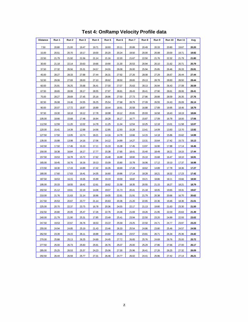
z
Test 4: OnRamp Velocity Profile data
Distance Run 1 Run 2 Run 3 Run 4 Run 5 Run 6 Run 7 Run 8 Run 9 Run 10 Run 11 Avg
7.50 20.80 21.00 19.47 19.71 18.93 20.11 20.89 20.49 20.33 20.80 19.67 20.20
15.00 20.51 20.70 19.17 19.00 20.20 20.24 19.50 20.00 20.08 20.00 19.71 19.92
22.50 21.79 21.92 21.56 21.14 21.16 22.20 21.67 22.50 21.76 22.32 21.79 21.80
30.00 21.18 22.14 20.63 19.66 19.90 21.30 20.53 20.94 20.10 21.62 20.71 20.79
37.50 27.32 26.56 25.31 24.57 24.55 26.08 26.00 25.94 25.85 26.46 26.33 25.91
45.00 28.27 28.33 27.88 27.44 26.31 27.92 27.26 28.08 27.29 26.67 26.44 27.44
52.50 29.06 27.69 28.00 27.10 28.62 28.50 28.65 29.13 28.78 28.83 28.50 28.44
60.00 25.91 26.25 25.68 26.41 27.00 27.07 25.63 28.13 26.94 26.43 27.08 26.59
67.50 28.65 28.99 28.17 28.55 27.97 28.81 28.43 28.41 27.90 28.61 28.06 28.41
75.00 28.27 28.69 27.45 25.16 28.86 27.50 27.73 27.86 28.88 28.59 26.35 27.76
82.50 26.08 24.46 24.55 26.25 25.54 27.68 28.79 27.09 26.55 24.43 26.09 26.14
90.00 20.07 17.72 18.87 18.89 18.44 18.91 20.58 16.88 17.89 19.95 18.46 18.79
97.50 19.30 18.18 19.12 17.78 18.98 19.12 20.65 20.93 16.58 18.43 18.19 18.84
105.00 18.66 15.68 17.48 16.94 18.28 16.17 16.77 15.87 17.09 16.78 18.00 17.06
112.50 12.59 11.20 12.02 14.78 11.25 11.34 12.54 10.25 12.18 13.01 11.58 12.07
120.00 15.41 14.39 12.68 14.56 12.85 12.93 15.28 13.41 14.09 13.83 13.70 13.92
127.50 17.50 13.05 13.74 18.21 14.16 14.78 13.66 14.15 14.18 15.86 15.62 14.99
135.00 15.88 13.98 14.16 17.06 14.12 14.89 14.27 13.31 15.64 17.42 15.73 15.13
142.50 17.50 17.46 15.10 17.11 15.19 15.38 17.45 13.97 16.90 17.88 17.14 16.46
150.00 18.38 16.84 16.17 17.77 15.38 17.65 18.41 15.40 18.49 18.21 19.15 17.44
157.50 19.53 16.78 15.72 17.62 15.48 16.88 18.60 15.10 15.68 16.47 18.10 16.91
165.00 18.45 16.76 16.16 19.13 15.09 15.80 15.78 16.06 17.12 19.10 17.37 16.98
172.50 18.30 17.43 14.89 17.42 16.35 18.69 17.28 18.62 14.89 17.78 18.36 17.27
180.00 17.60 17.63 16.41 14.35 16.60 19.86 17.14 18.28 18.21 18.32 17.23 17.42
187.50 18.53 16.15 19.35 15.99 19.19 19.59 18.82 19.21 18.86 18.11 19.66 18.50
195.00 20.33 18.55 18.42 12.61 18.62 21.58 18.35 20.55 21.15 18.27 18.21 18.79
202.50 21.12 19.61 22.19 14.06 19.07 21.73 20.41 21.18 18.05 19.65 19.31 19.67
210.00 21.76 21.63 21.14 18.96 19.05 22.81 21.91 21.79 20.38 20.66 16.70 20.62
217.50 20.53 20.67 23.77 21.14 20.63 20.36 21.20 22.65 22.36 19.46 18.36 21.01
225.00 20.70 22.37 23.75 16.78 20.36 24.55 22.17 21.13 19.80 21.63 23.30 21.50
232.50 20.80 20.05 25.47 17.26 22.76 24.46 21.69 19.26 21.95 22.03 20.63 21.49
240.00 21.79 21.90 25.31 17.85 23.49 25.41 23.94 22.50 23.20 24.89 22.93 23.02
247.50 19.53 22.67 26.76 18.53 23.22 25.59 23.25 22.50 24.71 24.77 23.97 23.23
255.00 24.94 24.85 25.19 21.43 23.46 26.33 25.54 24.86 23.80 25.46 24.57 24.58
262.50 23.39 24.15 26.11 18.88 24.60 25.66 23.57 23.81 26.71 26.34 25.36 24.42
270.00 25.88 25.13 26.25 24.69 24.45 27.72 26.65 25.76 24.69 26.76 25.00 25.72
277.50 25.00 26.73 25.60 25.91 26.76 25.07 25.00 25.29 27.86 27.66 27.00 26.17
285.00 25.25 26.53 25.37 24.23 25.06 27.30 25.96 26.41 27.26 26.25 27.32 26.09
292.50 26.44 26.59 25.77 27.31 26.46 24.77 26.02 24.41 25.96 27.42 27.14 26.21
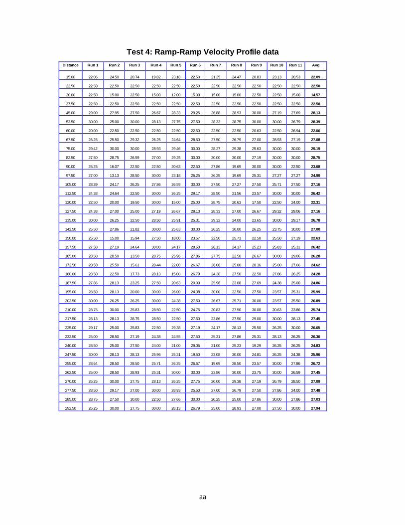
aa
Test 4: Ramp-Ramp Velocity Profile data
Distance Run 1 Run 2 Run 3 Run 4 Run 5 Run 6 Run 7 Run 8 Run 9 Run 10 Run 11 Avg
15.00 22.06 24.50 20.74 19.82 23.18 22.50 21.25 24.47 20.83 23.13 20.53 22.09
22.50 22.50 22.50 22.50 22.50 22.50 22.50 22.50 22.50 22.50 22.50 22.50 22.50
30.00 22.50 15.00 22.50 15.00 12.00 15.00 15.00 15.00 22.50 22.50 15.00 14.57
37.50 22.50 22.50 22.50 22.50 22.50 22.50 22.50 22.50 22.50 22.50 22.50 22.50
45.00 29.00 27.95 27.50 26.67 28.33 29.25 26.88 28.93 30.00 27.19 27.69 28.13
52.50 30.00 25.00 30.00 28.13 27.75 27.50 28.33 28.75 30.00 30.00 26.79 28.39
60.00 20.00 22.50 22.50 22.50 22.50 22.50 22.50 22.50 20.63 22.50 26.94 22.06
67.50 26.25 25.50 29.32 26.25 24.64 28.50 27.50 26.79 27.00 28.93 27.19 27.08
75.00 29.42 30.00 30.00 28.93 29.46 30.00 28.27 29.38 25.63 30.00 30.00 29.19
82.50 27.50 28.75 26.59 27.00 29.25 30.00 30.00 30.00 27.19 30.00 30.00 28.75
90.00 26.25 16.07 22.50 22.50 20.63 22.50 27.86 19.69 30.00 30.00 22.50 23.68
97.50 27.00 13.13 28.50 30.00 23.18 26.25 26.25 19.69 25.31 27.27 27.27 24.90
105.00 28.39 24.17 26.25 27.86 26.59 30.00 27.50 27.27 27.50 25.71 27.50 27.16
112.50 24.38 24.64 22.50 30.00 26.25 29.17 28.50 21.56 23.57 30.00 30.00 26.42
120.00 22.50 20.00 19.50 30.00 15.00 25.00 28.75 20.63 17.50 22.50 24.00 22.31
127.50 24.38 27.00 25.00 27.19 26.67 28.13 28.33 27.00 26.67 29.32 29.06 27.16
135.00 30.00 26.25 22.50 28.50 25.91 25.31 29.32 24.00 23.65 30.00 29.17 26.78
142.50 25.50 27.86 21.82 30.00 25.63 30.00 26.25 30.00 26.25 23.75 30.00 27.00
150.00 25.50 15.00 15.94 27.50 18.00 23.57 22.50 25.71 22.50 25.50 27.19 22.63
157.50 27.50 27.19 24.64 30.00 24.17 28.50 28.13 24.17 25.23 25.83 25.31 26.42
165.00 28.50 28.50 13.50 28.75 25.96 27.86 27.75 22.50 26.67 30.00 29.06 26.28
172.50 28.50 25.50 15.61 28.44 22.00 26.67 26.06 25.00 20.36 25.00 27.66 24.62
180.00 28.50 22.50 17.73 28.13 15.00 26.79 24.38 27.50 22.50 27.86 26.25 24.28
187.50 27.86 28.13 23.25 27.50 20.63 20.00 25.96 23.08 27.69 24.38 25.00 24.86
195.00 28.50 28.13 20.00 30.00 26.00 24.38 30.00 22.50 27.50 23.57 25.31 25.99
202.50 30.00 26.25 26.25 30.00 24.38 27.50 26.67 25.71 30.00 23.57 25.50 26.89
210.00 28.75 30.00 25.83 28.50 22.50 24.75 20.83 27.50 30.00 20.63 23.86 25.74
217.50 28.13 28.13 28.75 28.50 22.50 27.50 23.86 27.50 29.00 30.00 28.13 27.45
225.00 29.17 25.00 25.83 22.50 29.38 27.19 24.17 28.13 25.50 26.25 30.00 26.65
232.50 25.00 28.50 27.19 24.38 24.55 27.50 25.31 27.86 25.31 28.13 26.25 26.36
240.00 28.50 25.00 27.50 24.00 21.00 29.06 21.00 25.23 19.29 26.25 26.25 24.83
247.50 30.00 28.13 28.13 25.96 25.31 19.50 23.08 30.00 24.81 26.25 24.38 25.96
255.00 28.64 28.50 28.50 25.71 26.25 26.67 19.69 28.50 23.57 30.00 27.86 26.72
262.50 25.00 28.50 28.93 25.31 30.00 30.00 23.86 30.00 23.75 30.00 26.59 27.45
270.00 26.25 30.00 27.75 28.13 26.25 27.75 20.00 29.38 27.19 26.79 28.50 27.09
277.50 28.50 29.17 27.00 30.00 28.93 25.50 27.00 26.79 27.50 27.86 24.00 27.48
285.00 28.75 27.50 30.00 22.50 27.66 30.00 20.25 25.00 27.86 30.00 27.86 27.03
292.50 26.25 30.00 27.75 30.00 28.13 26.79 25.00 28.93 27.00 27.50 30.00 27.94
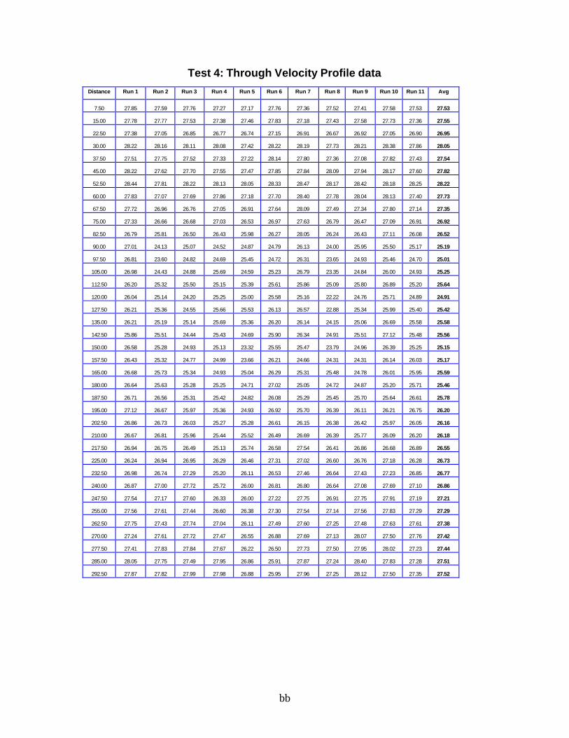
bb
Test 4: Through Velocity Profile data
Distance Run 1 Run 2 Run 3 Run 4 Run 5 Run 6 Run 7 Run 8 Run 9 Run 10 Run 11 Avg
7.50 27.85 27.59 27.76 27.27 27.17 27.76 27.36 27.52 27.41 27.58 27.53 27.53
15.00 27.78 27.77 27.53 27.38 27.46 27.83 27.18 27.43 27.58 27.73 27.36 27.55
22.50 27.38 27.05 26.85 26.77 26.74 27.15 26.91 26.67 26.92 27.05 26.90 26.95
30.00 28.22 28.16 28.11 28.08 27.42 28.22 28.19 27.73 28.21 28.38 27.86 28.05
37.50 27.51 27.75 27.52 27.33 27.22 28.14 27.80 27.36 27.08 27.82 27.43 27.54
45.00 28.22 27.62 27.70 27.55 27.47 27.85 27.84 28.09 27.94 28.17 27.60 27.82
52.50 28.44 27.81 28.22 28.13 28.05 28.33 28.47 28.17 28.42 28.18 28.25 28.22
60.00 27.83 27.07 27.69 27.86 27.18 27.70 28.40 27.78 28.04 28.13 27.40 27.73
67.50 27.72 26.96 26.76 27.05 26.91 27.64 28.09 27.49 27.34 27.80 27.14 27.35
75.00 27.33 26.66 26.68 27.03 26.53 26.97 27.63 26.79 26.47 27.09 26.91 26.92
82.50 26.79 25.81 26.50 26.43 25.98 26.27 28.05 26.24 26.43 27.11 26.08 26.52
90.00 27.01 24.13 25.07 24.52 24.87 24.79 26.13 24.00 25.95 25.50 25.17 25.19
97.50 26.81 23.60 24.82 24.69 25.45 24.72 26.31 23.65 24.93 25.46 24.70 25.01
105.00 26.98 24.43 24.88 25.69 24.59 25.23 26.79 23.35 24.84 26.00 24.93 25.25
112.50 26.20 25.32 25.50 25.15 25.39 25.61 25.86 25.09 25.80 26.89 25.20 25.64
120.00 26.04 25.14 24.20 25.25 25.00 25.58 25.16 22.22 24.76 25.71 24.89 24.91
127.50 26.21 25.36 24.55 25.66 25.53 26.13 26.57 22.88 25.34 25.99 25.40 25.42
135.00 26.21 25.19 25.14 25.69 25.36 26.20 26.14 24.15 25.06 26.69 25.58 25.58
142.50 25.86 25.51 24.44 25.43 24.69 25.90 26.34 24.91 25.51 27.12 25.48 25.56
150.00 26.58 25.28 24.93 25.13 23.32 25.55 25.47 23.79 24.96 26.39 25.25 25.15
157.50 26.43 25.32 24.77 24.99 23.66 26.21 24.66 24.31 24.31 26.14 26.03 25.17
165.00 26.68 25.73 25.34 24.93 25.04 26.29 25.31 25.48 24.78 26.01 25.95 25.59
180.00 26.64 25.63 25.28 25.25 24.71 27.02 25.05 24.72 24.87 25.20 25.71 25.46
187.50 26.71 26.56 25.31 25.42 24.82 26.08 25.29 25.45 25.70 25.64 26.61 25.78
195.00 27.12 26.67 25.97 25.36 24.93 26.92 25.70 26.39 26.11 26.21 26.75 26.20
202.50 26.86 26.73 26.03 25.27 25.28 26.61 26.15 26.38 26.42 25.97 26.05 26.16
210.00 26.67 26.81 25.96 25.44 25.52 26.49 26.69 26.39 25.77 26.09 26.20 26.18
217.50 26.94 26.75 26.49 25.13 25.74 26.58 27.54 26.41 26.86 26.68 26.89 26.55
225.00 26.24 26.94 26.95 26.29 26.46 27.31 27.02 26.60 26.76 27.18 26.28 26.73
232.50 26.98 26.74 27.29 25.20 26.11 26.53 27.46 26.64 27.43 27.23 26.85 26.77
240.00 26.87 27.00 27.72 25.72 26.00 26.81 26.80 26.64 27.08 27.69 27.10 26.86
247.50 27.54 27.17 27.60 26.33 26.00 27.22 27.75 26.91 27.75 27.91 27.19 27.21
255.00 27.56 27.61 27.44 26.60 26.38 27.30 27.54 27.14 27.56 27.83 27.29 27.29
262.50 27.75 27.43 27.74 27.04 26.11 27.49 27.60 27.25 27.48 27.63 27.61 27.38
270.00 27.24 27.61 27.72 27.47 26.55 26.88 27.69 27.13 28.07 27.50 27.76 27.42
277.50 27.41 27.83 27.84 27.67 26.22 26.50 27.73 27.50 27.95 28.02 27.23 27.44
285.00 28.05 27.75 27.49 27.95 26.86 25.91 27.87 27.24 28.40 27.83 27.28 27.51
292.50 27.87 27.82 27.99 27.98 26.88 25.95 27.96 27.25 28.12 27.50 27.35 27.52

cc
Test 4: Offramp Velocity Profile data
Distance Run 1 Run 2 Run 3 Run 4 Run 5 Run 6 Run 7 Run 8 Run 9 Run 10 Run 11 Avg
7.50 25.13 26.03 27.50 27.50 26.07 26.43 26.25 26.05 26.59 25.78 26.47 26.35
15.00 26.35 26.84 26.25 28.50 25.45 26.05 27.50 26.90 24.06 25.50 26.50 26.35
22.50 26.09 26.88 26.36 26.25 26.88 25.66 27.32 26.54 26.25 27.50 25.57 26.48
30.00 27.27 26.59 28.85 28.93 29.00 28.00 26.47 26.47 27.30 26.25 28.42 27.60
37.50 26.70 29.06 26.25 28.30 26.64 28.21 26.25 25.56 27.75 27.66 27.08 27.22
45.00 27.89 27.95 27.72 26.63 25.80 28.33 28.13 26.41 27.81 29.00 27.86 27.59
52.50 28.21 28.64 29.27 28.21 23.65 28.42 28.39 28.13 26.25 26.72 26.74 27.51
60.00 27.61 28.33 28.64 27.27 24.64 26.91 27.66 28.03 27.60 29.00 26.25 27.45
67.50 27.16 28.33 25.11 28.50 27.25 25.71 27.32 26.61 26.05 28.24 23.86 26.74
75.00 28.06 26.39 26.70 28.33 25.80 25.10 27.60 26.25 23.60 23.93 23.13 25.90
82.50 28.04 27.63 25.40 26.13 26.45 24.71 28.56 24.13 19.09 23.25 26.47 25.44
90.00 24.52 23.86 21.25 24.46 23.06 24.46 28.93 24.75 22.28 21.38 21.43 23.67
97.50 20.90 26.56 22.74 23.63 24.38 23.25 23.06 21.32 19.75 20.80 23.10 22.68
105.00 22.31 24.32 22.14 23.75 21.36 23.18 22.71 21.18 20.56 23.37 22.84 22.52
112.50 21.63 21.43 14.44 22.50 18.88 20.92 22.22 17.14 20.19 20.00 21.82 20.11
120.00 20.96 20.70 18.41 20.87 21.21 18.33 19.29 21.04 20.50 20.25 22.50 20.37
127.50 22.50 21.82 18.00 21.11 21.00 19.29 21.94 18.36 18.25 21.71 23.75 20.70
135.00 24.38 24.20 20.63 22.00 21.43 22.50 23.80 18.17 17.59 23.25 24.64 22.05
142.50 24.00 22.13 20.77 22.17 21.00 23.21 23.57 18.43 22.50 22.50 24.78 22.28
150.00 25.00 23.18 21.67 21.16 20.68 23.15 22.92 18.83 22.50 24.38 24.46 22.54
157.50 23.00 23.21 21.48 22.80 19.07 22.88 23.61 17.81 23.13 24.17 23.57 22.25
165.00 23.82 21.90 23.28 20.32 15.00 22.16 20.16 16.81 23.40 25.26 22.14 21.30
180.00 21.67 19.89 22.81 18.75 20.97 21.70 18.50 19.93 21.88 21.75 23.13 21.00
187.50 21.63 23.93 22.50 15.77 21.35 22.50 20.28 21.62 23.75 18.75 22.50 21.32
195.00 24.26 22.20 22.50 20.74 17.73 24.46 20.48 20.40 23.00 17.50 21.25 21.32
202.50 24.11 25.18 25.80 20.00 23.13 24.87 21.43 20.92 22.50 22.50 22.17 22.96
210.00 25.20 24.20 24.64 19.57 26.37 24.55 20.83 23.64 23.93 22.92 24.17 23.64
217.50 24.30 26.25 23.10 21.29 25.67 25.96 24.00 25.40 27.14 23.86 25.18 24.74
225.00 25.78 26.07 25.00 22.00 23.75 26.41 21.00 23.18 20.77 20.63 24.11 23.52
232.50 27.40 24.64 24.17 20.80 22.25 27.00 20.83 21.56 20.92 26.79 25.66 23.82
240.00 26.41 27.24 21.43 19.80 24.57 27.50 19.14 24.11 24.46 25.00 21.90 23.78
247.50 25.45 27.63 25.80 21.09 23.65 24.75 15.58 26.25 24.29 27.92 23.61 24.18
255.00 26.90 27.86 25.00 22.50 23.37 24.13 20.77 26.79 23.71 25.38 21.43 24.35
262.50 27.00 27.50 25.10 21.25 23.08 26.43 23.41 24.44 24.38 27.92 24.64 25.01
270.00 27.14 29.12 22.50 23.70 26.94 26.25 19.90 25.63 22.21 27.50 26.43 25.21
277.50 28.70 28.88 23.25 24.19 25.23 28.33 20.36 25.71 22.86 28.59 26.40 25.68
285.00 27.08 29.25 20.00 22.50 25.83 27.75 25.00 26.47 27.61 27.86 27.12 26.04
292.50 27.61 28.27 24.44 20.63 25.71 28.82 25.34 27.81 26.70 28.33 26.05 26.34
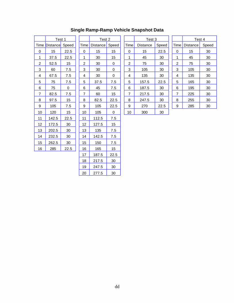
dd
Single Ramp-Ramp Vehicle Snapshot Data
Test 1 Test 2 Test 3 Test 4
Time Distance Speed Time Distance Speed Time Distance Speed Time Distance Speed
0 15 22.5 0 15 15 0 15 22.5 0 15 30
1 37.5 22.5 1 30 15 1 45 30 1 45 30
2 52.5 15 2 30 0 2 75 30 2 75 30
3 60 7.5 3 30 0 3 105 30 3 105 30
4 67.5 7.5 4 30 0 4 135 30 4 135 30
5 75 7.5 5 37.5 7.5 5 157.5 22.5 5 165 30
6 75 0 6 45 7.5 6 187.5 30 6 195 30
7 82.5 7.5 7 60 15 7 217.5 30 7 225 30
8 97.5 15 8 82.5 22.5 8 247.5 30 8 255 30
9 105 7.5 9 105 22.5 9 270 22.5 9 285 30
10 120 15 10 105 0 10 300 30
11 142.5 22.5 11 112.5 7.5
12 172.5 30 12 127.5 15
13 202.5 30 13 135 7.5
14 232.5 30 14 142.5 7.5
15 262.5 30 15 150 7.5
16 285 22.5 16 165 15
17 187.5 22.5
18 217.5 30
19 247.5 30
20 277.5 30
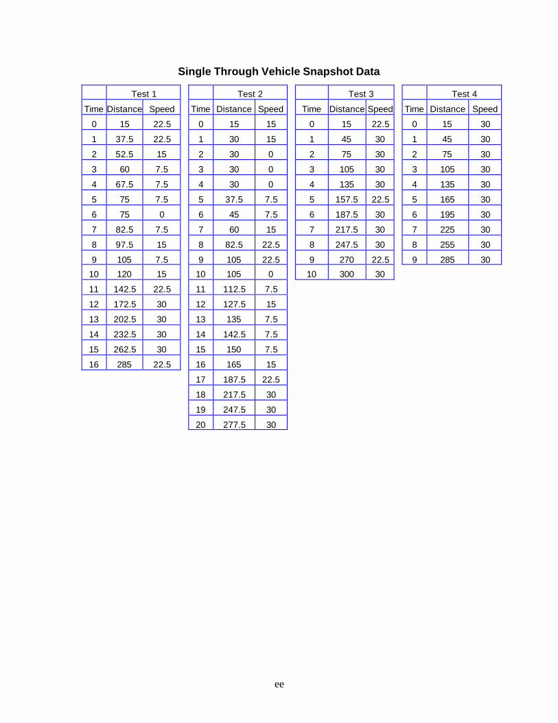
ee
Single Through Vehicle Snapshot Data
Test 1 Test 2 Test 3 Test 4
Time Distance Speed Time Distance Speed Time Distance Speed Time Distance Speed
0 15 22.5 0 15 15 0 15 22.5 0 15 30
1 37.5 22.5 1 30 15 1 45 30 1 45 30
2 52.5 15 2 30 0 2 75 30 2 75 30
3 60 7.5 3 30 0 3 105 30 3 105 30
4 67.5 7.5 4 30 0 4 135 30 4 135 30
5 75 7.5 5 37.5 7.5 5 157.5 22.5 5 165 30
6 75 0 6 45 7.5 6 187.5 30 6 195 30
7 82.5 7.5 7 60 15 7 217.5 30 7 225 30
8 97.5 15 8 82.5 22.5 8 247.5 30 8 255 30
9 105 7.5 9 105 22.5 9 270 22.5 9 285 30
10 120 15 10 105 0 10 300 30
11 142.5 22.5 11 112.5 7.5
12 172.5 30 12 127.5 15
13 202.5 30 13 135 7.5
14 232.5 30 14 142.5 7.5
15 262.5 30 15 150 7.5
16 285 22.5 16 165 15
17 187.5 22.5
18 217.5 30
19 247.5 30
20 277.5 30
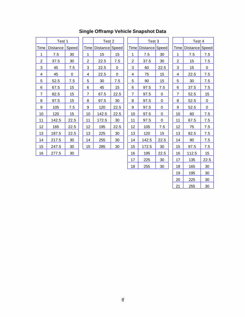
ff
Single Offramp Vehicle Snapshot Data
Test 1 Test 2 Test 3 Test 4
Time Distance Speed Time Distance Speed Time Distance Speed Time Distance Speed
1 7.5 30 1 15 15 1 7.5 30 1 7.5 7.5
2 37.5 30 2 22.5 7.5 2 37.5 30 2 15 7.5
3 45 7.5 3 22.5 0 3 60 22.5 3 15 0
4 45 0 4 22.5 0 4 75 15 4 22.5 7.5
5 52.5 7.5 5 30 7.5 5 90 15 5 30 7.5
6 67.5 15 6 45 15 6 97.5 7.5 6 37.5 7.5
7 82.5 15 7 67.5 22.5 7 97.5 0 7 52.5 15
8 97.5 15 8 97.5 30 8 97.5 0 8 52.5 0
9 105 7.5 9 120 22.5 9 97.5 0 9 52.5 0
10 120 15 10 142.5 22.5 10 97.5 0 10 60 7.5
11 142.5 22.5 11 172.5 30 11 97.5 0 11 67.5 7.5
12 165 22.5 12 195 22.5 12 105 7.5 12 75 7.5
13 187.5 22.5 13 225 30 13 120 15 13 82.5 7.5
14 217.5 30 14 255 30 14 142.5 22.5 14 90 7.5
15 247.5 30 15 285 30 15 172.5 30 15 97.5 7.5
16 277.5 30 16 195 22.5 16 112.5 15
17 225 30 17 135 22.5
18 255 30 18 165 30
19 195 30
20 225 30
21 255 30
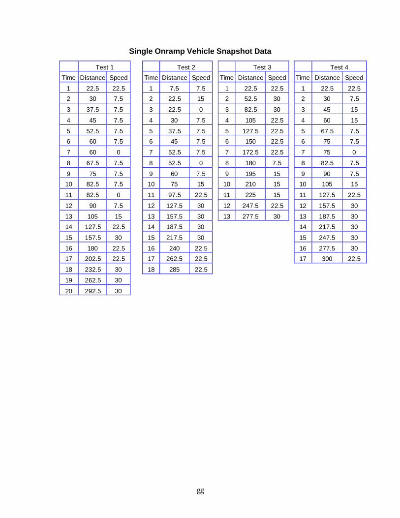
gg
Single Onramp Vehicle Snapshot Data
Test 1 Test 2 Test 3 Test 4
Time Distance Speed Time Distance Speed Time Distance Speed Time Distance Speed
1 22.5 22.5 1 7.5 7.5 1 22.5 22.5 1 22.5 22.5
2 30 7.5 2 22.5 15 2 52.5 30 2 30 7.5
3 37.5 7.5 3 22.5 0 3 82.5 30 3 45 15
4 45 7.5 4 30 7.5 4 105 22.5 4 60 15
5 52.5 7.5 5 37.5 7.5 5 127.5 22.5 5 67.5 7.5
6 60 7.5 6 45 7.5 6 150 22.5 6 75 7.5
7 60 0 7 52.5 7.5 7 172.5 22.5 7 75 0
8 67.5 7.5 8 52.5 0 8 180 7.5 8 82.5 7.5
9 75 7.5 9 60 7.5 9 195 15 9 90 7.5
10 82.5 7.5 10 75 15 10 210 15 10 105 15
11 82.5 0 11 97.5 22.5 11 225 15 11 127.5 22.5
12 90 7.5 12 127.5 30 12 247.5 22.5 12 157.5 30
13 105 15 13 157.5 30 13 277.5 30 13 187.5 30
14 127.5 22.5 14 187.5 30 14 217.5 30
15 157.5 30 15 217.5 30 15 247.5 30
16 180 22.5 16 240 22.5 16 277.5 30
17 202.5 22.5 17 262.5 22.5 17 300 22.5
18 232.5 30 18 285 22.5
19 262.5 30
20 292.5 30
hh
Vita
Srinivas Jillella was born on January 18, 1978 in Hyderabad, India. He graduated with a
Bachelor in Technology degree in Civil Engineering from Indian Institute of Technology,
Bombay, India in 1999. He started his work towards his Masters Degree in Civil
Engineering at Virginia Polytechnic Institute and State University in the fall of 1999.
Srinivas is currently working with Exeter at Cambridge, Massachusetts since July 2001.