Embed Size (px)
Citation preview

Testing the Prebisch-Singer Hypothesis since
1650: Evidence from Panel Techniques that
Allow for Multiple Breaks
Rabah Arezki, Kaddour Hadri, Prakash Loungani, Yao Rao

© 2013 International Monetary Fund WP/13/180
IMF Working Paper
Research Department
Testing the Prebisch-Singer Hypothesis since 1650: Evidence from Panel Techniques that
Allow for Multiple Breaks
Prepared by Rabah Arezki, Kaddour Hadri, Prakash Loungani, Yao Rao1
Authorized for distribution by Prakash Loungani
August 2013
Abstract
In this paper, we re-examine two important aspects of the dynamics of relative primary
commodity prices, namely the secular trend and the short run volatility. To do so, we employ
25 series, some of them starting as far back as 1650 and powerful panel data stationarity tests
that allow for endogenous multiple structural breaks. Results show that all the series are
stationary after allowing for endogeneous multiple breaks. Test results on the Prebisch-
Singer hypothesis, which states that relative commodity prices follow a downward secular
trend, are mixed but with a majority of series showing negative trends. We also make a first
attempt at identifying the potential drivers of the structural breaks. We end by investigating
the dynamics of the volatility of the 25 relative primary commodity prices also allowing for
endogenous multiple breaks. We describe the often time-varying volatility in commodity
prices and show that it has increased in recent years.
JEL Classification Numbers: O13, C22.
Keywords: Primary commodities; Unit root tests; Multiple Structural breaks ; Volatility.
Author’s E-Mail Address: [email protected]; [email protected]; [email protected];
1 International Monetary Fund; Queen.s University; International Monetary Fund; and Liverpool Management
School, respectively. Hadri.s research was partly supported by the British Academy under the Japan-Britain
Research Cooperative Program. The authors are grateful to the participants at the IMF Research Department and
Oxford University conference on "Understanding International Commodity Price Fluctuations" held March 20-21,
2013 in Washington, DC.
This Working Paper should not be reported as representing the views of the IMF.
The views expressed in this Working Paper are those of the author(s) and do not necessarily
represent those of the IMF or IMF policy. Working Papers describe research in progress by the
author(s) and are published to elicit comments and to further debate.

1 Introduction
The present paper re-examines two important aspects of the dynamics of rela-tive primary commodity prices using long time series, some of them starting asfar back as 1650. The dynamics of relative primary commodity prices can be de-composed into essentially three components: The secular trend which Prebisch(1950) and Singer (1950) have conjectured should be declining, the long cyclesthat a¤ect relative primary commodity prices and �nally the volatility which hasbeen found often time varying and generally increasing in recent years.2 In thispaper, we do not examine the long cycles component for lack of space (cf. Ertenand Ocampo, 2012 and references therein). We focus on the Prebisch-Singerhypothesis (thereafter PSH) and the volatility of relative primary commodityprices using recent panel data technology.The �rst step in testing the PSH is to test for the stationarity of the series.
This is important because depending on whether or not the series are stationarywe must use the appropriate regression framework to test for the PSH. If yt, thelogarithm of the relative commodity price is generated by a stationary processaround a time trend, then the following equation is:
yt = �+ �t+ "t; t = 1; : : : ; T; (1)
where t is a linear trend and the random variable "t is stationary with mean0 and variance �2". The parameter of interest is the slope �, which is predictedto be negative under the PSH. If the real commodity prices were generated bya so called di¤erence-stationary or I(1) (thereafter DS) model, implying that ytis non-stationary, then we should employ the following equation:
�yt = � + vt; t = 1; : : : ; T; (2)
where vt is stationary. It is well known that if yt is a DS process, then usingequation (1) to test the null hypothesis of � = 0 will result in acute size dis-tortions, leading to a wrong rejection of the null when no trend is present, evenasymptotically. Alternatively, if the true generating process is given by equation(1) and we base our test on equation (2), our test becomes ine¢ cient and lesspowerful than the one based on the correct equation. Therefore, when testingthe PSH we have �rst to test the order of integration of our relative commodityprices in order to use the right regression. In this paper, we use the Hadri andRao (2008) panel stationarity test in order to test jointly for the stationarityof our series, in turn increasing the power of the test relatively to individuallytesting each time series. Using the Hadri and Rao (2008) panel stationarity testalso allows us to incorporate the information contained in the cross sectionaldependence of our series. It is well known that there are generally positive andsigni�cant correlations between real primary commodity prices. Pindyck andRotemberg (1990) noted this strong correlation in the real prices of unrelatedcommodities which they refer to as "excess co-movement". They found that
2See Hadri (2011) for an analysis of the implications of these components for policymakers.
2

even after controlling for current and expected future values of macroeconomicvariables this excess co-movement remains.We use long time series, some of them starting in 1650. It is thus highly
likely that they will show multiple breaks. Since the pioneering work of Perron(1989), it is widely accepted that the failure of taking into account structuralbreaks is likely to lead to a signi�cant loss of power in unit root tests. Similarly,stationarity tests ignoring the existence of breaks diverge and thus are biasedtoward rejecting the null hypothesis of stationarity in favour of the false alter-native of a unit root hypothesis. This is due to severe size distortion caused bythe presence of breaks (see inter alia Lee et al. (1997). Therefore in our panelstationarity tests, we allow for endogenous multiple breaks in order to avoidbiases in our tests. The other innovation in this paper compared to most previ-ous papers is that not only do we use very long series but we also use relativeprimary commodity prices instead of aggregate indices. By doing so, we avoidthe aggregation bias and the generally ad-hoc weighting rule to combine thecommodity prices involved.The �nal step deals with testing the signi�cance and�nding the sign of the slopes of the appropriate regressions in order to �nd outif the PSH is not rejected by the data. We also make a �rst attempt at identi-fying the potential drivers of those breaks by exploiting information related tothe break dates and the change of the signs in the piecewise regressions of thetrend.We end by examining the volatility of primary commodity prices. It is well
known that primary commodity prices are highly volatile (c.f. Mintz, 1967,Reinhart and Wickham, 1994 and for oil, Dvir and Rogo¤, 2009). Using longseries, we also test for data driven structural breaks in volatility employing Baiand Perron (1998) methodology.
2 Panel stationarity tests with multiple struc-tural breaks
In this paper, we extend Hadri and Rao (2008) to deal with multiple breaks.In Hadri and Rao (2008) we considered four possibilities of e¤ects that a singlebreak may cause on the deterministic parts of the model under the null hypothe-sis. Model 0 has a break in the level (�i) and no trend (�i = 0). Model 1 allowsfor a break in the level and a time trend without a break ("crash model" inPerron�s terminology) and model 2 permits a break in the slope only. In model3, a break is admitted in both the level and the slope. Model 3 is the mostgeneral model which encompasses the three other models. Model 3 is speci�edas follows:
Model 3: yit = �i + rit + �iDit(!�) + �it+ iDTit(!
�) + �it; (3)
withrit = rit�1 + uit; (4)
3

where yit; i = 1; :::; N cross-section units and t = 1; :::; T time periods, are theobserved series for which we wish to test stationarity. For all i; �0is, �
0is, �
0is and
0is are unknown parameters. rit is a random walk with initial values ri0 = 08i: DTit(!�) = t� T � when t > T � and 0 otherwise, Dit(!�) = 1 if t = T � + 1and 0 otherwise, with T � = [!�T ] the break date with the associated breakfraction !��(0; 1) and [.] denotes the integer part of the argument.Under thenull hypothesis of yit being stationary rit reduces to zero and Model 3 becomes:
yit = �i + �iDit(!�) + �it+ iDTit(!
�) + �it;
For testing the PSH on the basis of the general to speci�c methodology weshall be using solely model 3. Within the panel data framework, two modelsamong the four models proposed in Hadri and Rao (2008) were able to allow formultiple breaks (see also Carrion-i-Silvestre, Del Barrio and López-Bazo (2005),thereafter CDL). Each of the two models is based on di¤erent break e¤ects, i.e.breaks in the level and no trend (model 0) and breaks in both the level and thetrend (model 3). The general model considered here can be written as follows:
yi;t = �i;t + �it+ "i;t;
�i;t =
miXk=1
�i;kDUi;k;t +
miXk=1
i;kD(Tib;k)t + �i;t�1 + �i;t;
where �i;t s i:i:d(0; �2v;i); "i;t is allowed to be serially correlated. f�i;tg andf"i;tg are assumed to be mutually independent across i and over t: This as-sumption is relaxed later to allow for cross-sectional dependence. D(T ib;k)t andDUi;k;t are de�ned as D(T ib;k)t = 1 for t = T ib;k + 1 and 0 elsewhere, andDUi;k;t = 1 for t > T ib;k and 0 elsewhere with T
ib;k denoting the kth date of
break for the ith individual, k = 1; :::;mi: The null hypothesis is speci�ed as�2v;i = 0 for all i; under which we obtain:
yi;t = �i +
miXk=1
�i;kDUi;k;t + �it+
miXk=1
i;kD(Tib;k)t + �i;t: (5)
Hence, model 0 is obtained when �i = i;k = 0; and model 3 is de�ned if �i 6= 0and i;k 6= 0, �i is the initial value of �i;t:The proposed test statistic, which is based on the Hadri (2000) LM test, is
expressed as:
LM(�) = N�1NXi=1
(!�2i T�2TXt=1
S2i;t); (6)
where S2i;t =tX
j=1
"i;t denotes the partial sum of OLS estimated residuals "i;t. For
each i, �i = (�i;1; :::; �i;mi)0= (T ib;1=T; ::; T
ib;mi
=T )0 indicates the locations of thebreaks over T: Since autocorrelation is allowed in the residuals, !2i is a consistent
4

long-run variance (LRV) estimate of "i;t for each i. To obtain a consistentestimator of !2i ; we use a nonparametric method jointly with the boundarycondition rule suggested by Sul et al. (2003) which is shown to be e¤ectivein avoiding inconsistency problems in the KPSS-type test. Using appropriatemoments and applying a Central Limit Theorem (CLT), the limiting distributionof the statistic (6) is shown to be a standard normal, that is,
Z(�) =
pN(LM(�)� ��)
�&=) N(0; 1);
with
�� = N�1NXi=1
�i; &2 = N�1
NXi=1
&2i :
The asymptotic mean and variances for each individual have been provided inCBL (2005) as follows:
�i = A
mi+1Xk=1
(�i;k � �i;k�1)2; &2i = Bmi+1Xk=1
(�i;k � �i;k�1)4:
The values of A and B equal the values of moments in Hadri (2000), that is, formodel 0, A = 1
6 ; B =145 ; for model 3, A =
115 ; B =
116300 :
In the situation where break dates are unknown, the SSR procedure is em-ployed to estimate the break points, that is, the estimated break dates are ob-tained by minimizing the sum of squared residuals. To estimate multiple breakdates we employ the method of Bai and Perron (1998) that computes the globalminimization of the sum of squared residuals (SSR), so that all the break datesare estimated via minimizing the sequence of individual SSR(T ib;1; :::; T
ib;mi
)computed from (5)
(T ib;1; :::; Tib;mi
) = arg minT ib;1;:::;T
ib;mi
SSR(T ib;1; :::; Tib;mi
):
2.1 Testing the presence of multiple structural changes
In order to obtain a consistent estimation of the number and dates of the breakswe have �rst to test for the presence of breaks in the series of interest. Bai andPerron (1998) suggest a sup Wald type test for the null hypothesis of no changeagainst an alternative containing an arbitrary number of changes. They alsopropose a sequential test. In this paper, we use the double maximum tests whichhave the advantage that a pre-speci�cation of a particular number of breaks isnot required before testing the signi�cance of the breaks. Therefore, we can testthe null hypothesis of no structural break against an unknown number of breakswith given bound M of number of breaks. It is pointed out by Perron (2005)that double maximum tests can play a signi�cant role in testing for structuralchanges and they are the most useful tests to apply when we want to determineif structural changes are present. In addition, it is also shown in Bai and Perron
5

(2005) by simulations that the double maximum tests is as powerful as the bestpower that can be achieved using the test that accounts for the correct numberof breaks. For the Double maximum tests, the UDmax and WDmax are usedand are de�ned as follows:
UDmaxFT (M; q) = max1�m�M
sup(�1;:::;�m)2��
FT (�1; :::; �m; q)
WDmaxFT (M; q) = max1�m�M
c(q; �; 1)
c(q; �;m)� sup(�1;:::;�m)2��
FT (�1; :::; �m; q)
The UDmax is an equal version of double maximum tests which assuming equalweights to the possible number of structural changes. And WDmax appliesweights to the individual tests such that the marginal p-values are equal acrossvalues of number of breaks. The values of these two tests are reported in theappropriate tables. All the UDmax and WDmax tests are signi�cant at 1%signi�cance level . This clearly shows that at least one structural break is presentfor any of the real primary commodity price.
3 Data
We employ 25 relative commodity prices constructed by Harvey, Kellard Madsenand Wohar (2010)3 . They calculate these relative commodity prices by de�atingthe nominal commodity series with the manufacturing value-added price index.Eight relative commodity prices cover the period 1650-2005. These are: Beef,lamb, lead, sugar, wheat, wool, coal and gold. We call this set 1.The relativeprices of aluminum, cocoa, co¤ee, copper, cotton, hide, rice, silver, tea, tin,tobacco, zinc, pig iron, nickel, and oil cover the period 1872-2005. We call thisset 2, the set including all the commodity prices for which we have observationsduring the period 1872-2005 including set 1. Finally, the relative commodityprices of banana and jute cover the period 1900-2005. We call this set 3, thebalanced panel including all the 25 relative commodity prices covering the period1900-2005. Figure 1 shows the evolution of the natural logarithm of the 25relative commodity prices covering the period 1900-2005. Table 1 gives thecross-sectional correlations between all the commodity prices. Overall, pricesof the various commodities are positively and highly correlated indicating thepresence of a common component.
3We thank David Harvey for providing the data.
6

Figure 1. Evolution of relative primary commodity prices
0500
01000
015
000
2000
0AL
UM
INU
M
1600 1700 1800 1900 2000year
Aluminium
010
0200
3004
00BA
NA
NA
1600 1700 1800 1900 2000year
Banana
010
0200
3004
00BE
EF
1600 1700 1800 1900 2000year
Beef
050
0100
0150
0C
OC
OA
1600 1700 1800 1900 2000year
Cocoa
050
0100
01500
CO
FFEE
1600 1700 1800 1900 2000year
Coffee50
10015
020025
0300
CO
PPER
1600 1700 1800 1900 2000year
Copper
050
0010
000
CO
TTO
N
1600 1700 1800 1900 2000year
Cotton
050
0100
0150
0H
IDE
1600 1700 1800 1900 2000year
Hide
02004
006008
00100
0JU
TE
1600 1700 1800 1900 2000year
Jute
050
1001
5020
0LA
MB
1600 1700 1800 1900 2000year
Lamb
010
0200
3004
00LE
AD
1600 1700 1800 1900 2000year
Lead
010
0020
0030
00R
ICE
1600 1700 1800 1900 2000year
Rice
050
0100
0150
0SI
LVER
1600 1700 1800 1900 2000year
Silver
0200
040006
00080
00SU
GA
R
1600 1700 1800 1900 2000year
Sugar
0500
01000
015
000
2000
0TE
A
1600 1700 1800 1900 2000year
Tea
010
0200
3004
00TI
N
1600 1700 1800 1900 2000year
Tin
010
0200
3004
00TO
BAC
CO
1600 1700 1800 1900 2000year
Tobacco
05001
00015
00200025
00W
OO
L
1600 1700 1800 1900 2000year
Wool
050
0100
0150
0W
HE
AT
1600 1700 1800 1900 2000year
Wheat
020
040
060
0ZI
NC
1600 1700 1800 1900 2000year
Zinc
050
1001
5020
0PI
G IR
ON
1600 1700 1800 1900 2000year
Pig Iron
5010
015
020
0C
OAL
1600 1700 1800 1900 2000year
Coal
020
040
060
0N
ICK
EL
1600 1700 1800 1900 2000year
Nickel50
10015
020025
0300
GO
LD
1600 1700 1800 1900 2000year
Gold
020
0400
6008
00O
IL
1600 1700 1800 1900 2000year
Oil
7

4 Empirical Results
4.1 Testing the Prebisch-Singer hypothesis
4.1.1 Testing the stationarity of relative commodity prices
The �rst step when testing the PSH is to test for the stationarity of the seriesin order to use the right equation to estimate the signi�cance and the sign ofthe coe¢ cient of the time trend �: As explained above, we employ a panelstationarity test allowing for serial correlation, cross-sectional dependence andendogenous multiple breaks. The maximum breaks allowed are speci�ed asmmax = 5 and 8: But we report only mmax = 5 as the di¤erence between thetwo sets of results is negligible. The numbers of breaks are determined by usingthe modi�ed Schwarz Information Criterion (LWZ). The Bootstrap method isemployed to correct for cross-sectional dependence. The critical values, withnumbers of replications equal to 5000, are reported in the tables below. Thecorrection for cross-sectional dependence is essential as the relative commodityprices have been shown in Table 1 to be highly correlated.The following tables summarize the results of break mmax = 5 estimations.
To make the best use of the information contained in the data, we considerthree sets of data. In Table 2 we report the results of the panel stationaritytests for 25 commodities prices for the period 1900-2005. We �rst test forthe presence of structural breaks in the series using UDmax and WDmax :Both tests are signi�cant at 1% signi�cance level. This clearly shows that atleast one structural break is present for all the relative primary commodityprices. (Similar results apply for the other sets and therefore we do not reportthe critical values). Then we determine the number of breaks and the breakdates. The bootstrap critical values show clearly that the null hypothesis ofjoint stationarity of the series is not rejected at the 5% and 10% levels. InTables 3 and 4 we carry the same tests for respectively set 1 and set 2 andfor both the null hypothesis of joint stationarity of the series is not rejectedat the the 5% and 10% levels. Finally, Tables 5, 6 and 7 report the piecewiseregressions for respectively set 3, set 1 and set 2.
8
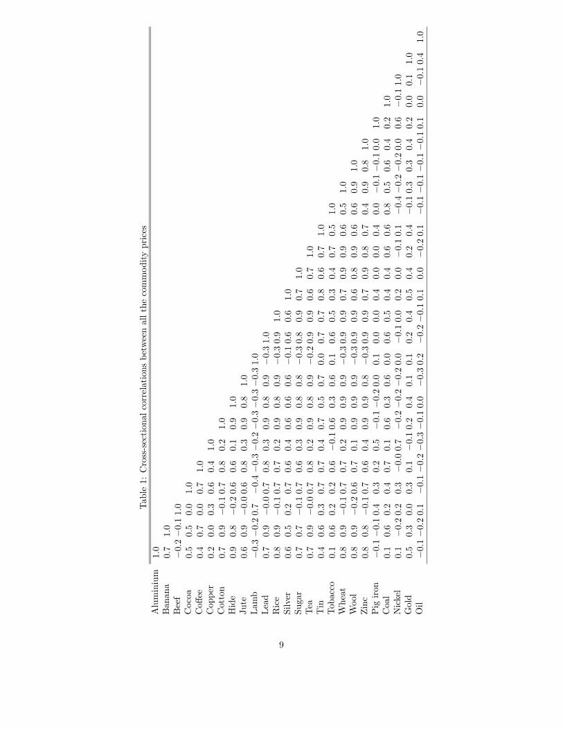
Table1:Cross-sectionalcorrelationsbetweenallthecommodityprices
Aluminium
Banana
Beef
Cocoa
Co¤ee
Copper
Cotton
Hide
Jute
Lamb
Lead
Rice
Silver
Sugar
TeaTinTobacco
Wheat
Wool
Zinc
Pigiron
Coal
Nickel
Gold
Oil
1:0
0:7
1:0
�0:2�0:11:0
0:5
0:5
0:0
1:0
0:4
0:7
0:0
0:7
1:0
0:2
0:0
0:3
0:6
0:4
1:0
0:7
0:9
�0:10:7
0:8
0:2
1:0
0:9
0:8
�0:20:6
0:6
0:1
0:9
1:0
0:6
0:9
�0:00:6
0:8
0:3
0:9
0:8
1:0
�0:3�0:20:7
�0:4�0:3�0:2�0:3�0:3�0:31:0
0:7
0:9
�0:00:7
0:8
0:3
0:9
0:8
0:9
�0:31:0
0:8
0:9
�0:10:7
0:7
0:2
0:9
0:8
0:9
�0:30:9
1:0
0:6
0:5
0:2
0:7
0:6
0:4
0:6
0:6
0:6
�0:10:6
0:6
1:0
0:7
0:7
�0:10:7
0:6
0:3
0:9
0:8
0:8
�0:30:8
0:9
0:7
1:0
0:7
0:9
�0:00:7
0:8
0:2
0:9
0:8
0:9
�0:20:9
0:9
0:6
0:7
1:0
0:4
0:6
0:3
0:7
0:7
0:4
0:7
0:5
0:7
0:0
0:7
0:7
0:8
0:6
0:7
1:0
0:1
0:6
0:2
0:2
0:6
�0:10:6
0:3
0:6
0:1
0:6
0:5
0:3
0:4
0:7
0:5
1:0
0:8
0:9
�0:10:7
0:7
0:2
0:9
0:9
0:9
�0:30:9
0:9
0:7
0:9
0:9
0:6
0:5
1:0
0:8
0:9
�0:20:6
0:7
0:1
0:9
0:9
0:9
�0:30:9
0:9
0:6
0:8
0:9
0:6
0:6
0:9
1:0
0:8
0:8
�0:10:7
0:6
0:4
0:9
0:9
0:8
�0:30:9
0:9
0:7
0:9
0:8
0:7
0:4
0:9
0:8
1:0
�0:1�0:10:4
0:3
0:2
0:5
�0:1�0:20:0
0:1
0:0
0:0
0:4
0:0
0:0
0:4
0:0
�0:1�0:10:0
1:0
0:1
0:6
0:2
0:4
0:7
0:1
0:6
0:3
0:6
0:0
0:6
0:5
0:4
0:4
0:6
0:6
0:8
0:5
0:6
0:4
0:2
1:0
0:1
�0:20:2
0:3
�0:00:7
�0:2�0:2�0:20:0
�0:10:0
0:2
0:0
�0:10:1
�0:4�0:2�0:20:0
0:6
�0:11:0
0:5
0:3
0:0
0:3
0:1
�0:10:2
0:4
0:1
0:1
0:2
0:4
0:5
0:4
0:2
0:4
�0:10:3
0:3
0:4
0:2
0:0
0:1
1:0
�0:1�0:20:1
�0:1�0:2�0:3�0:10:0
�0:30:2
�0:2�0:10:1
0:0
�0:20:1
�0:1�0:1�0:1�0:10:1
0:0
�0:10:4
1:0
9

Table 2. Summary of estimated numbers and location of structural breaks(mmax=5)
(25 commodities from 1900-2005, set 3)Commodities Estimated Break Dates (mmax = 5) UDmax WDmax
TB1 TB2 TB3 TB4 TB5Aluminum 1918 1941 78.26 171.84Banana 1916 1931 1971 238.01 425.41Beef 1950 1965 140.58 177.83Cocoa 1947 1973 1989 85.27 187.22Co¤ee 1949 1987 131.79 175.55Copper 1947 1975 111.57 141.14Cotton 1930 1946 319.80 568.25Hide 1921 1952 32.57 35.92Jute 1947 104.15 209.73Lamb 1935 1950 1965 285.48 427.24Lead 1947 1982 120.11 151.94Rice 1982 75.66 113.09Silver 1940 1979 139.94 177.02Sugar 1925 1965 1982 31.01 68.08Tea 1922 1954 1986 321.52 571.30Tin 1986 75.54 95.56
Tobacco 1918 1968 497.30 629.10Wheat 1946 34.91 57.25Wool 1948 1991 187.97 237.78Zinc 1918 1948 23.42 46.14
Pig Iron 1933 1948 1987 56.43 100.28Coal 1966 1984 166.29 365.12Nickel 1931 1950 1991 142.47 312.81Gold 1917 1934 1957 1979 288.03 632.42Oil 1946 1974 1991 76.22 122.49
Panel Stationarity test Statistics Value Bootstrap Critical Values10% 5%
Homogeneous variance 5.498 12.521 12.911Heterogeneous variance 3.009 4.939 5.414
10

Table 3. Summary of estimated numbers and location of structural breaks(mmax=5)
(8 commodities from 1650-2005, set 1 )Commodities Estimated Break Dates (mmax = 5)
TB1 TB2 TB3 TB4 TB5Beef 1793 1876 1952Lamb 1793 1894 1947Lead 1721 1793 1851 1946Sugar 1833Wheat 1837 1945Wool 1793 1875 1947Coal 1892 1952Gold 1793 1913
Panel Stationarity test Statistics Value Bootstrap Critical Values10% 5%
Homogeneous variance 0.176 2.706 3.290Heterogeneous variance 2.207 2.526 3.096
11

Table 4. Summary of estimated numbers and location of structural breaks(mmax=5)
(23 commodities from 1872-2005, set 2)Commodities Estimated Break Dates (mmax = 5)
TB1 TB2 TB3 TB4 TB5Aluminum 1891 1918 1940Beef 1949 1969Cocoa 1907 1946 1985Co¤ee 1949Copper 1898 1946 1974Cotton 1945Hide 1920 1951Lamb 1934 1955Lead 1946 1981Rice 1981Silver 1939 1978Sugar 1928 1981Tea 1922 1953 1985Tin 1985
Tobacco 1894 1917 1967Wheat 1945Wool 1947 1982Zinc 1917 1947
Pig Iron 1948 1985Coal 1964 1984Nickel 1899 1949Gold 1916 1938 1958 1978Oil 1915 1973
Panel Stationarity test Statistics Value Bootstrap Critical Values10% 5%
Homogeneous variance 1.849 4.380 5.103Heterogeneous variance 2.624 3.988 4.619
4.1.2 Piecewise regressions
After determining the presence, the numbers and the locations of structuralbreaks for the above relative commodity prices, we consider piecewise regressionsto examine the signs, the signi�cance and change of signs over time of theslopes of these regressions. The logarithm of the relative commodity prices areused in the regressions. For each commodity we �t a linear trend model, i.e.,yt = �+ �t+ "t before and after the break dates. The results are summarizedin tables 5, 6 and 7 for the three sets considered in this paper. �m representsthe estimated slope for the linear regression model before the mth structuralbreak. The values in bracket are the p-values for the corresponding parameters.
12

Table 5. Piecewise regression results (mmax=5)(25 commodities from 1900-2005, set 3)
Commodities Piecewise Regression�1 �2 �3 �4 �5
Aluminum -0.03�(0.01) -0.01(0.18) -0.01�(0.00)Banana 0.01(0.00) 0.04(0.00) -0.02�(0.00) -0.02�(0.00)Beef 0.01(0.00) 0.12(0.00) -0.03�(0.00)Cocoa -0.04�(0.00) -0.02�(0.00) -0.05�(0.00) 0.004(0.32)Co¤ee -0.006�(0.02) -0.02�(0.00) -0.044�(0.00)Copper -0.02�(0.00) 0.02(0.00) -0.02�(0.00)Cotton 0.00(0.19) 0.01(0.21) -0.04�(0.00)Hide 0.02(0.00) -0.001(0.39) -0.02�(0.00)Jute -0.01�(0.00) -0.04�(0.00)Lamb 0.02(0.00) -0.07�(0.00) 0.12(0.00) -0.01�(0.01)Lead -0.01�(0.00) -0.02�(0.00) -0.01(0.17)Rice -0 .01�(0.00) -0.01(0.21)Silver -0.02�(0.00) 0.02(0.00) -0.08�(0.00)Sugar -0.004(0.27) -0.002(0.30) 0.04(0.09) -0.02�(0.00)Tea -0.04�(0.00) -0.004(0.18) -0.05�(0.00) -0.01(0.12)Tin 0.001(0.18) -0.02�(0.00)
Tobacco 0.004(0.07) 0.003(0.049) -0.03�(0.00)Wheat -0.02�(0.00) -0.03�(0.00)Wool -0.006�(0.00) -0.05�(0.00) 0.02(0.05)Zinc 0.02(0.03) 0.00(0.49) -0.02�(0.00)
Pig Iron -0.014�(0.00) -0.04�(0.00) 0.01(0.00) 0.003(0.36)Coal 0.01(0.00) 0.02(0.01) -0.02�(0.01)Nickel -0.04�(0.00) -0.04�(0.00) 0.01(0.00) 0.03(0.02)Gold -0.02�(0.00) 0.02(0.00) -0.05�(0.00) 0.01(0.02) -0.03�(0.00)Oil 0.01(0.00) -0.02�(0.00) -0.02(0.17) 0.05(0.00)
13

Table 6. Piecewise regression results (mmax=5)(8 commodities from 1650-2005, set 1 )
Commodities Piecewise Regression�1 �2 �3 �4 �5
Beef 0.002(0.00) 0.014(0.00) -0..002�(0.03) -0.01�(0.02)Lamb 0.001(0.00) 0.014(0.00) 0.02(0.00) 0.018(0.00)Lead -0.01�(0.00) 0.00(0.05) 0.01(0.00) -0.01�(0.00) -0.03�(0.00)Sugar -0.003�(0.00) -0.02�(0.00)Wheat 0.00(0.00) -0.01�(0.00) -0.03�(0.00)Wool -0.002�(0.00) 0.02(0.00) -0.01�(0.00) -0.05�(0.00)Coal 0.001(0.00) 0.01(0.00) -0.02�(0.00)Gold 0.001(0.001) 0.01(0.00) -0.003�(0.01)
14

Table 7. Piecewise regression results (mmax=5)(23 commodities from 1872-2005, set 2)
Commodities Piecewise Regression�1 �2 �3 �4 �5
Aluminum -0.03�(0.003) -0.07�(0.00) -0.01(0.18) -0.012�(0.00)Beef 0.00(0.358) 0.10(0.00) -0.04�(0.00)Cocoa 0.01(0.002) -0.04�(0.00) -0.01�(0.04) -0.02�(0.012)Co¤ee -0.01�(0.00) -0.04�(0.00)Copper -0.02�(0.00) -0.02�(0.00) 0.02(0.00) -0.02�(0.00)Cotton -0.01�(0.00) -0.04�(0.00)Hide 0.002(0.14) -0.001(0.39) -0.02�(0.00)Lamb 0.001(0.16) -0.10�(0.00) 0.00(0.46)Lead -0.004�(0.00) -0.02�(0.00) -0.01(0.17)Rice -0.01�(0:00) -0.01(0.21)Silver -0.024�(0.00) 0.02(0.00) -0.08�(0.00)Sugar -0.02�(0.00) -0.003(0.22) -0.02�(0.00)Tea -0.03�(0.00) -0.01�(0.01) -0.05�(0.00) -0.01(0.12)Tin 0.004(0.00) -0.02�(0.00)
Tobacco 0.05(0.00) -0.00(0.35) 0.003(0.05) -0.03�(0.00)Wheat -0.012�(0.00) -0.03�(0.00)Wool -0.01�(0.00) -0.05�(0.00) -0.02�(0.02)Zinc 0.001(0.294) 0.00(0.49) -0.02�(0.00)
Pig Iron -0.01�(0.00) 0.01(0.00) -0.004(0.32)Coal 0.01(0.00) 0.01(0.17) -0.012�(0.05)Nickel -0.07�(0.00) -0.02�(0.00) 0.002(0.16)Gold 0.00(0.37) 0.04(0.00) -0.05�(0.00) 0.02(0.01) -0.04�(0.00)Oil -0.02�(0.00) -0.02�(0.00) -0.02�(0.02)
15

4.1.3 Analysis of the results of the Prebisch-Singer testing
Tables 2 and 5 report the results for set 3. Table 2 indicates the timing and thenumber of breaks for the 25 primary commodities whereas Table 5 shows thecorresponding signi�cance and sign of the slopes of the piecewise regressions.Four commodities have 1 break, thirteen have 2 breaks, seven register 3 breaksand only one (gold) has 4 breaks. Out of the total of 80 slope estimates, 41 arenegative and signi�cant, 11 are negative but insigni�cant, 21 are positive andsigni�cant �nally, 7 are positive and insigni�cant. Tables 3 and 6 concern set 1.One commodity has one break (sugar), three commodities have 2 breaks, threeother commodities are a¤ected by 3 breaks and one commodity has 4 breaks.Of the 27 slope estimates, 13 are negative and signi�cant, 13 other are positiveand signi�cant and one is positive but insigni�cant. Table 4 and Table 7 dealwith set 2. Five commodities have one break, twelve have 2 breaks, �ve have 3breaks and one commodity has four breaks. Of the 71 slope estimates. forty fourare negative and signi�cant, 7 are negative but insigni�cant, 11 are positive andsigni�cant and 9 are positive but insigni�cant. These results seem to indicatethat in the majority of cases the PSH is not rejected.
4.1.4 Drivers of structural breaks
We make a �rst attempt at identifying the potential drivers of those breaksby simply matching breaks to historical events(see Appendix Table). For theinvestigation of the drivers of the breaks, we shall consider for each commodityprice only its longest series. The appendix table presents a tentative list ofdrivers behind those breaks based on historical accounts of the development inprimary commodity markets. We draw from various sources including Radetzki(2011). In the following, we summarize the main take aways from those historicaldevelopments which help explain the presence of breaks in commodity pricesseries.The share of the primary sector in GDP has declined steadily overtime in
advanced economies (see Radetzki, 2011). Recently, most of the total consump-tion growth of primary commodities has taken place in emerging economies likeChina. For instance, its share of total consumption growth in this century was50%. In the case of copper China�s utilization between 2000 and 2008 corre-sponds to 113% of total increase Cochilco (2009). Also, China�s import growthof iron ore between 2000 and 2009 corresponded to 125% of total import growth(UNCTAD, 2010). The decline in the share of the commodity sector in GDPcan also be explained by the growing ability to create man made substitutes.Another aspect analysed by Radetzki (2011) is the role of relentlessly falling
transport costs in shaping and expanding primary commodity markets sincethe 19th century. Up to mid-19th century, shipment rates on long hauls wereprohibitively high. Only high value primary commodities like co¤ee, cocoa,spices and precious or semi-precious metals could be transported. However,towards the end of the second-half of the 19th century, the use of the steamtechnology made long hauls transport more a¤ordable and bene�ted primary
16

commodities like cotton, wheat and wool. Also, the introduction around 1880sof refrigeration made possible the transport of meat and fruit over long distances.Between 1950 and 1970 steady improvements in specialized bulk carriers leadto dramatic fall in the transport costs of heavy primary commodities like ironore, coal, bauzite and oil.Finally, state intervention starting early 1930s and beginning to fade in 1970s
may had some e¤ects on the formation of prices of primary commodities. Radet-zki (2011) considers four main factors explaining state intrusion in primary com-modity production and commerce: (1) the Great Depression of 1930s led to theprice collapse of many primary commodities like wheat, sugar and rubber. (2)the second world war provoked havoc in the supply routes of numerous com-modities including sugar, wheat, co¤ee and tin. (3) the breakup of colonialempires a¤ected greatly the functioning of primary commodity markets (buy-ing at above market prices, food aid...), (4) the period 1925 to 1975 witnessedthe wide spread belief in collectivism. But since the 1980s government controlstarted to fade except notably in oil industries where it remains strong.The appendix tables provide numerous examples of cases where we identi�ed
that changes in transportation technology and in the structure of commoditymarkets coincide with structural breaks in commodity prices.
4.2 Volatility of relative commodity prices
We now turn to examining the volatility of commodity prices. As in Dvirand Rogo¤ (2009), we de�ne volatility as the mean absolute residual from aregression of a given relative primary commodity price growth on its laggedvalue. It is well documented that primary commodity prices are relatively highlyvolatile and this volatility is time varying (Mintz (1967), Reinhart and Wickham(1994) and Dvir and Rogo¤ (2009) for oil). In contrast, manufactured goodprices have been found to be less volatile. By volatility, we refer to short termmovements of primary commodity prices to be distinguished from medium andlong term cycles that are another characteristics of primary commodity prices.It has also been found that commodity price variability is large relatively to thesecular trend.In order to �nd periods of high price instability, we test for multiple breaks in
commodity price volatility employing the methods proposed by Bai and Perron(1998, 2003).The results are reported graphically below
4.2.1 Analysis of the volatility results
Ten price volatilities are found without breaks. These include copper, pig iron,silver, tin, banana, co¤ee, jute, tobacco, wheat, and oil. This is surprisingparticularly concerning the price volatility of oil which is perceived to be veryvolatile. Dvir and Rogo¤ (2009) �nd three break points for the price volatilityof oil. However, it should be noted that (1) they use real oil price whereas weuse oil price relative to a price index of manufactures, (2) they consider theperiod 1861-2008, while we use observations starting in 1874 and ending in 2005
17

and (3) the results may depend on the various criteria used by Bai and Perron(2008) which do not always agree as noted by Dvir and Rogo¤ (2009). Eightprice volatilities are a¤ected by one break: gold in 1932, lead in 1913, cocoa in1913, rice in 1965, sugar in 1912, beef in 1913, lamb in 1914 and coal in 1704.Three primary commodity relative price volatilities indicates two breaks. Theseare; nickel (1902 and 1985), zinc (1911 and 1938), hide (1917 and 1938), wool(1713 and 1966). Finally, only aluminium has three break points in 1904, 1923and 1986. Some more research is needed to �nd the cause of these breaks. Ingeneral, it seems that volatility has increased for most primary commodities inrecent years.In this section, we do not attempt to match systematically the breaks in
the volatility in commodity price series with historical developments. However,we summarize the main �ndings from the literature on the potential drivers ofvolatility.Cashin and McDermott (2002) describe primary commodity price volatil-
ities as rapid, unexpected and often as large changes in primary commodityprices. They noted an increase in the amplitude of price movements around1899. Some authors found that since the breakdown of the Bretton Woodsexchange regime, real commodity prices have exhibited increasing variabilitysince early 1970 (Chu and Morrisson (1984), Reinhart and Wickham (1994) andCuddington and Liang (1999)). The price elasticity of demand for raw materi-als is generally small because its cost represents only a tiny fraction of the �nalproduct price. Therefore, an increase in the demand for �nished products willcause a greater increase in the demand for the primary materials used due to
18

19

20

the necessary increase of inventories of �nished product which will a¤ect theentire production chain.Fluctuations in supply also contribute to price volatility. The weather is a
factor that can a¤ect the price stability of agricultural products although itsimportance has diminished in recent decades due to the geographical diversi�-cation of production. Important strikes or major technical accidents can be thecause of signi�cant decrease in mineral supply. The price elasticity of supplyis generally low, particularly at around full capacity which is often the case incompetitive markets. Consequently, it takes considerable time to increase sup-ply capacity and in the interim even tiny variations in demand will result inconsiderable change in price. Wars or expected wars are another cause of sharpchange in primary commodity prices.Since World War II, three commodity booms have occurred, 1950, 1973 and
2003 (see Radetzki, 2006). They were all generated by demand shocks dueto rapid macroeconomic expansion. The �rst two commodity booms subsidedin 1952 and 1974 respectively, less than two years after their birth. Duringthe more recent boom, prices increased sharply (food prices by more than 50%and fuel prices doubled) from 2003 and lasted until the �rst-half of 2008. Thiswas followed in the second-half of 2008 by a severe global contraction whichstayed until the end of 2009. Then, commodity prices increased dramaticallyagain. This commodity price recovery is thought to be due to the major emerg-ing economies and possibly to slack monetary policy and the recent in�ows ofspeculative capital into commodity markets.
21

22

23

24

25

26

27

28

29

5 Conclusions
In this paper, we re-examined the Prebisch-Singer hypothesis employing 25 rel-ative primary commodity prices observed over more than three-and-half cen-turies. We found that all the series are stationary employing powerful panelstationarity tests accounting for data driven structural breaks. The results onthe Prebisch-Singer hypothesis tests are mixed. However, the majority of thepiecewise regressions have downward slopes. We also reviewed some potentialdrivers of structural breaks.We also investigated the volatility and data drivenstructural breaks of primary commodity prices. Primary commodity prices arefound to be highly volatile with often time varying volatility. In general thevolatility has the tendency to increase during the recent years.
30

References
[1] Atkinson, G., and K. Hamilton (2003). Savings, Growth and ResourceCurse Hypothesis. World Development, 31(11), 1793-1807.
[2] Bai, J. and P. Perron (1998). Estimating and Testing Linear Models withMultiple Structural Changes, Econometrica, 66, 47-78.
[3] Bai, J. and P. Perron (2008). Computation and Analysis of Multiple Struc-tural Change Models, Journal of Applied Econometrics, 18, 1-22.
[4] Breitung, J. and Pesaran, M. H. (2008). Unit roots and cointegration inpanels. In: L. Matyas and P. Sevestre (eds): The Econometrics of PanelData: Fundamentals and Recent Developments in Theory and Practice.Dordrecht: Kluwer Academic Publishers, 3rd edition, Chapt. 9, pp. 279-322.
[5] Cashin, P. and J. McDermott (2002). The Long-Run Behavior of Com-modity Prices: Small Trends and Big Variability. IMF Sta¤ Papers, 44(2),175-199.
[6] Chu, Keyoung, and T.K. Morrison (1984). The 1981-82 Recession and Non-Oil Primary Commodity Prices. IMF Sta¤ Papers, Vol. 31 (March), pp.93-140.
[7] Christiano, L., and T.J. Fitzgerald (2003), The Bandpass Filter, Interna-tional Economic Review, 44. 435-465.
[8] Cochilco (2009), Yearbook: Copper and other mineral statistics 1989-2008(Santiago Comision del Cobre).
[9] Cuddington, J., and H. Liang (1999). Commodity Price Volatility AcrossExchange Rate Regimes. (unpublished, Washington: Department of Eco-nomics, Georgetown University).
[10] Cuddington, J., and D. Jerret (2008). Super Cycles in Metal Prices?, IMFSta¤ Papers, 55(4), 541-565.
[11] Deaton, A., (1999). Commodity Prices and Growth in Africa, Journal ofEconomic Perspective, 13, 23-40.
[12] Dvir, E., and K.S. Rogo¤ (2009). The threeEpochs of Oil Working paper posted on line athttp://www.economics.harvard.edu/�les/faculty/51_Three_Epochs_of_Oil.pdf.
[13] Erten, B. and J.A. Ocampo. (2012). Super-cycles of commodity prices sincethe mid-nineteenth century. DESAWorking Paper No. 110. United Nations,New York.
31

[14] Grilli, R.E., and M.C. Yang (1988). Commodity Prices, Manufacturedgoods Prices, and the terms of trade of Developing Countries. World BankEconomic Review, 2, 1-48.
[15] Frankel, J. (2010). A Solution to Fiscal Procyclicity: The Structural BudgetInstitutions Pioneered by Chile. Manuscript.
[16] Hadri, K. (2000). Testing for stationarity in heterogeneous panel data.Econometrics Journal 3, 148-161.
[17] Hadri, K. and Larsson, R (2005). Testing for stationarity in heterogeneouspanel data where the time dimension is �nite. Econometrics Journal 8,55-69.
[18] Hadri, K and Y. Rao (2008). Panel stationarity test with structural breaks.Oxford Bulletin of Economics and Statistics 70, 245-269.
[19] Hadri K. (2011) "Primary Commodity Price Series: Lessons for Policy-makers in Ressource-Rich Countries", in Beyond the Curse: Policies toHarness the Power of Natural Resources, R. Arezki, T. Gylfason & A. Sy,eds. (IMF, 2011). Invited address, High Level Seminar, IMF Institute &Central Bank of Algeria, Algiers 2010. Chap. 7, 119-130
[20] Hamilton, K. and J.M. Hartwick, (2005). Investing Exhaustible ResourceRents and the Path of Consumption. Canadian Journal of Economics. Vol.38, No. 2, pp. 615-621.
[21] Hartwick, J. (1977). Intergenerational Equity and the Investing of Rentsfrom Exhaustible Resources. The American Economic Review, 66, 972-4.
[22] Harvey, D. I., S. J. Leybourne, and A. M. R. Taylor, (2007). A Simple, Ro-bust and Powerful Test of the Trend Hypothesis. Journal of Econometrics,141 , 1302�1330.
[23] Harvey, D. I., S. J. Leybourne, and A. M. R. Taylor, (2009). Simple, Robustand Powerful Tests of the Breaking Trend Hypothesis. Econometric Theory,25, 995�1029.
[24] Harvey, D.I., N.M. Kellard, J.B. Madsen, and M.E. Wohar (2010). ThePrebisch-Singer Hypothesis: Four Centuries of Evidence, The review ofEconomics and Statistics, 92(2), 367-377.
[25] Hotteling, H. (1931). The Economics of Exhaustible Resources. Journal ofPolitical Economy, 39(2), 137-75.
[26] Kellard, N., and M.E. Wohar (2006). On the prevalence of trends in Pri-mary Commodity Prices, Journal of Development Economics, 79, 146-167.
[27] Kim, T., Pfa¤enzeller, S., Rayner, A., Newbold, P. (2003). Testing forlinear trend with application to relative primary commodity prices. Journalof Time Series Analysis, 24, 539-551.
32

[28] Lange and Wright (2004). Sustainable development in mineral economies:the example of Botswana. Environment and Development Economics, 9,485�505.
[29] Lewis, (1954). Economic Development with Unlimited Supplies of Labour,Manchester School of Economics and Social Studies, 22, 139-191.
[30] Mintz, I. (1967) Cyclical Fluctuations in the Exports ofthe United States Since 1879. NBER book. Volume URL:http://www.nber.org/books/mint67-1.
[31] Perron, P., (1989). The Great Crash, the Oil Price Shock, and the UnitRoot Hypothesis. Econometrica, 57, 1361-1401.
[32] Pindyck, R.S., and J.J. Rotember (1990). The Excess Co-Movements ofCommodity Prices. The Economic Journal, 100, 1173-1189.
[33] Prebisch, R., (1950). The Economic Development of Latin America and ItsPrincipal Problems. Economic Bulletin for Latin America, 7, 1-12.
[34] Radetzki, M. (2006). The anatomy of Three Commodity Booms. ResourcesPolicy, Vol.31, September.
[35] Radetzki, M. (2011) "Primary Commodities: Historical Perspectives andProspects", in Beyond the Curse: Policies to Harness the Power of Nat-ural Resources, R. Arezki, T. Gylfason & A. Sy, eds. (IMF, 2011). Invitedaddress, High Level Seminar, IMF Institute & Central Bank of Algeria,Algiers 2010. Chap. 3, 35-51.
[36] Reinhart, C., and P. Wickham (1994). Commodity Prices: Cyclical Weak-ness or Secular Decline? MPRA paper No. 8173 posted on line at:http://mpra.ub.uni-muenchen.de/8173/
[37] Rodríguez, J.C., Tokman, C.R., and Vega, A.C. (2007). Structural BalancePolicy in Chile, Published by the Budget O¢ ce of the Finance Ministry ofChile, available at: www.dipres.cl
[38] Singer, H., (1950). The Distribution of Gains between Investing and Bor-rowing Countries, American Economic review, Papers and Proceedings, 40,473-485.
[39] UNCTAD Report (2008). The Least Developed Countries. United Nations,New York.
[40] UNCTAD (2010). Iron Ore marker 2009-2011 (Geneva).
33

Beef16502005
1793Start of the IndustrialRevolution
1876First shipment offrozen beefarrived in NewOrleans(June1869); steamtechnology
1952Specialised bulk carrier
Lamb16502005
1793Start of the Industrialrevolution
1894Steam technologyand refrigeration
1947Specialised bulk carrierand refrigeration
Lead16502005
1721End of war between Russiaand Sweden, South Seabubble
1793Start of theIndustrialRevolution
1851Invention of battery(lead plates)
1946Specialized bulkcarrier
Sugar16502005
1833Abolition of slavery in theBritish empire(the sugar canetrade of the 18th and 19th
century relied on slavelabour)
Wheat16502005
1837Poor wheat harvest in GreatBritain; improvement intransport (canals in the US).
1945End of secondworld war,improvement intransport.
Wool16502005
1793Start of the IndustrialRevolution;Production of wool inAustralia
1875Loss of shipstransporting woolfrom Australia;bad weather alsohamperedtransport of wool
1947Abnormal demand forwool; Decrease in woolproduction in Australiaand South Africa due todrought; Decline in U.S.production
Coal16502005
1892Coal Creek War; Postwarrailroad construction,meanwhile, had opened upthe state's coalfields to majormining operations; Coalstrike in UK
1952Treatyestablishing theEuropean Coaland SteelCommunity;Specialized bulkcarrier
Gold16502005
1793Start of the IndustrialRevolution
1913The FederalReserve wasinstituted inDecember 1913;The last of thetrue GoldCertificates
Aluminium18722005
1891First used for building asteam passenger boat in1891; The Cowles processincreased dramatically the
1918Use of Duraluminin aviation ;First World War
1940Greater use ofaluminium; SecondWorld War
34

Cocoa18722005
1907Boycott against Portuguesecontinued used of slavery togrow cocoa in West Africa
1946Ghana CocoaBoard (1947);Ghana is thesecond largestproducer ofcocoa; End ofWorld War II
1985Major plantation fires inIvory Coast
Coffee18722005
1949The Havana charter onprimary commodityagreement;Improvement in transporttechnology
Copper18722005
1898A financial and commodityderivatives trading platformheadquartered in Chicago; InAlaska found a high gradedeposit of copper
1946End of World WarII
1974The price of copperreached a pick(commodity boom)
Cotton18722005
1945End of World War II
Hide18722005
1920Depression of 1920–21created a shock inagricultural commodityprices
1951Trade Agreementbetween India andPakistan
Rice18722005
1981Dramatic decline in prices
Silver18722005
1939The Great Depression
1978Attempt to cornerthe silver market
Tea18722005
1922 1953Tea Act 1953
1985Price peaked at 165pence/kg in October1989; the highest levelsince October 1985.
Tin18722005
1985Market collapse of themarket of tin due to thefailure of the InternationalTin Agreement
Tobacco18722005
1894F –Billmyer Warehouse(destroyed by arson in1894); Start of productionof tobacco in New Zeland
1917End of FirstWorld War
19671965: The FederalCigarette Labeling andadvertising Act is passedrequiring healthwarnings on cigarettepackages; As many as10,000,000 Americans
35

Zinc18722005
1917End of First World War
1947,End of SecondWorld War
Pig iron18722005
1948End of the Second WorldWar
1985
Nickel18722005
1899 1949Reconstructionafter SecondWorld War
Oil18722005
1915First world war
1973Oil embargoshock
Banana19002005
1916Banana wars
1931The Bananamassacre inColombia onDecember 6,1928,The Banana Wars
1971The period since 1971has seen major changesin both the world bananaeconomy and theeconomic environmentwithin which bananaproduction and tradetake place (The world ofeconomy 19701984,FAO economic andsocial development.
Jute19002005
1947The jute industry wasaffected greatly by theindependence of India andPakistan in 1947.
36