Local stationarity and time-inhomogeneous Markov chains

Lionel Truquet ∗†

Abstract

In this paper, we study a notion of local stationarity for discrete time Markov chains which is usefulfor applications in statistics. In the spirit of some locally stationary processes introduced in the literature,we consider triangular arrays of time-inhomogeneous Markov chains, defined by some families of con-tracting Markov kernels. Using the Dobrushin’s contraction coefficients for various metrics, we showthat the distribution of such Markov chains can be approximated locally with the distribution of ergodicMarkov chains and we also study some mixing properties. From our approximation results in Wasser-stein metrics, we recover several properties obtained for autoregressive processes. Moreover, using thetotal variation distance or more generally some distances induced by a drift function, we consider newmodels, such as finite state space Markov chains with time-varying transition matrices or some time-varying versions of integer-valued autoregressive processes. For these two examples, nonparametrickernel estimation of the transition matrix is discussed.

1 Introduction

Time-inhomogeneous Markov chains have received much less attention in the literature than the homoge-neous case. Such chains have been studied mainly for their long-time behavior, often in connexion with theconvergence of stochastic algorithms. An introduction to inhomogeneous Markov chains and their use inMonte Carlo methods can be found in Winkler (1995). More recent quantitative results for their long timebehavior can be found for instance in Douc et al. (2004), Saloff-Coste and Zúñiga (2007), or Saloff-Costeand Zúñiga (2011). In this paper, we consider convergence properties of nonhomogeneous Markov chainsbut with a different perspective, motivated by applications in mathematical statistics and in the spirit of thenotion of local stationarity introduced by Dahlhaus (1997). Locally stationary processes have received aconsiderable attention over the last twenty years, in particular for their ability to model data sets for whichtime-homogeneity is unrealistic. Locally stationary autoregressive processes (here with one lag for sim-plicity) can be defined by modifying a recursive equation followed by a stationary process. If (Xk)k∈Z is astationary processes defined by Xk = Fθ (Xk−1, εk), where (εk)k∈Z is a sequence of i.i.d random variables andθ ∈ Θ is a parameter, its locally stationary version is usually defined recursively by

Xn,k = Fθ(k/n)(Xn,k−1, εk

), 1 ≤ k ≤ n,

where θ : [0, 1] → Θ is a smooth function. This formalism was exploited for defining locally stationaryversions of classical time-homogeneous autoregressive processes. See for instance Dahlhaus and Subba Rao(2006), Subba Rao (2006) or Vogt (2012). The term local stationarity comes from the fact that, under some

∗UMR 6625 CNRS IRMAR, University of Rennes 1, Campus de Beaulieu, F-35042 Rennes Cedex, France and†Campus de Ker-Lann, rue Blaise Pascal, BP 37203, 35172 Bruz cedex, France. Email: lionel.truquet@ensai.fr.

1

regularity conditions, if k/n is close to a point u of [0, 1], Xn,k is close in some sense to Xk(u) where (Xk(u))k∈Zis the stationary process defined by

Xk(u) = Fθ(u) (Xk−1(u), εk) , k ∈ Z.

Though local stationary processes defined recursively are examples of time-inhomogeneous Markov chains,the properties of these processes are usually derived using this particular autoregressive representation andwithout exploiting the link with Markov chains. This is one the main difference with respect to stationaryprocesses for which the connection between autoregressive processes and Markov chains has been widelyused. See for example the classical textbook of Meyn and Tweedie (2009) for many examples of iterativesystems studied using Markov chains properties. As a limitation, the simple case of a locally stationaryversion of finite state space Markov chains has not been considered in the literature.

In this paper, we consider general Markov chains models which will generalize the existing (Marko-vian) locally stationary processes. Since we do not work directly with autoregressive representations, ourdefinition of local stationarity is based on the approximation of the finite dimensional distributions of thechain with that of some ergodic Markov chains. Let us now give the framework used in the rest of the paper.Let (E, d) be a metric space, B(E) its corresponding Borel σ−field and Qu : u ∈ [0, 1] a family of Markovkernels on (E,B(E)). By convention, we set Qu = Q0 when u < 0. We will consider triangular arraysXn, j : j ≤ n, n ∈ Z+

such that for all n ∈ Z+, the sequence

(Xn, j

)j≤n

is a non homogeneous Markov chainsuch that

P(Xn,k ∈ A|Xn,k−1 = x)

)= Qk/n(x, A), k ≤ n.

In the sequel the family Qu : u ∈ [0, 1] of Markov kernels will always satisfy some regularity conditionsand contraction properties. Precise assumptions will be given in three following sections, but from now on,we assume here that for all u ∈ [0, 1], Qu has a single invariant probability denoted by πu. For all positiveinteger j and all integer k such that k + j− 1 ≤ n, we denote by π(n)

k, j the probability distribution of the vector(Xn,k, Xn,k+1, . . . , Xn,k+ j−1

)and by πu, j the corresponding finite dimensional distribution for the ergodic chain

with Markov kernels Qu. Loosely speaking, the triangular array will be said locally stationary if for allpositive integer j, the probability distribution π(n)

k, j is close to πu, j when the ratio k/n is close to u. A formaldefinition is given below. For an integer j ≥ 1, we denote by P(E j) the set of probability measures on E j.

Definition 1. The triangular array of non-homogeneous Markov chainsXn,k, n ∈ Z+, k ≤ n

is said to be

locally stationary if for all integer j ≥ 1, there exists a metric ϑ j on P(E j

), metrizing the topology of weak

convergence, such that the two following conditions are satisfied.

1. The application u 7→ πu, j is continuous.

2. limn→∞

supk≤n− j+1

ϑ j

(π(n)

k, j, π kn , j

)= 0

In particular, under the two conditions of Definition 1, for all continuous and bounded function f : E j →

R and some integers k = kn ≤ n − j + 1 such that limn→∞ k/n = u ∈ [0, 1], we have

limn→∞E f

(Xn,k, . . . , Xn,k+ j−1

)= lim

n→∞f dπ(n)

k, j = E f(X1(u), . . . , X j(u)

)=

∫f dπu, j,

where (Xk(u))k∈Z denotes a stationary Markov chain with transition Qu. In this paper, Condition 1 willalways hold from the Hölder continuity properties that we will assume for the application u 7→ Qu. Of

2

course, the metrics ϑ j will of the same nature for different integers j, e.g the total variation distance onP(E j).

In this paper, we will consider three type of metrics onP(E) for approximating π(n)k by πk/n or πu (and in a

second step for approximating an arbitrary finite dimensional distribution) and deriving mixing properties ofthese triangular arrays. We will extensively make use of the so-called Dobrushin’s contraction coefficient. InSection 2, we consider the total variation distance. This is the metric for which the contraction coefficient forMarkov kernels has been originally introduced by Dobrushin (1956). Contraction properties of the kernelsQu or their iteration with respect to this metric will enable us to consider a model of nonhomogeneous finitestate space Markov chains for which we will study a nonparametric estimator of the time-varying transitionmatrix. In Section 3, we consider contraction properties for Wasserstein metrics. The contraction coefficientfor the Wasserstein metric of order 1 has been first considered by Dobrushin (1970) for giving sufficientconditions under which a system of conditional distributions defines a unique joint distribution. We willconsider more generally the Wasserstein metric of order p ≥ 1. This type of metric is very well adaptedfor recovering some results obtained for autoregressive processes with time-varying coefficients. Finally,in Section 4, we consider Markov kernels satisfying drift and minoration conditions ensuring geometricergodicity and for which Hairer and Mattingly (2011) have recently found a contraction property for ametric induced by a modified drift function. We illustrate this third approach with the statistical inferenceof some integer-valued autoregressive processes with time-varying coefficients.

2 Total variation distance and finite state space Markov chains

Let us first give some notations that we will extensively use in the sequel. If µ ∈ P(E) and R is a probabilitykernel from (E,B(E)) to (E,B(E)), we will denote by µR the probability measure defined by

µR(A) =

∫R(x, A)dµ(x), A ∈ B(E).

Moreover if f : E → R is a measurable function, we set µ f =∫

f dµ and R f : E → R will be the functiondefined by R f (x) =

∫R(x, dy) f (y), x ∈ E, provided these integrals are well defined. Finally, the Dirac

measure at point x ∈ E is denoted by δx.

2.1 Contraction and approximation result for the total variation distance

The total variation distance between two probability measures µ, ν ∈ P(E) is defined by

‖µ − ν‖TV = supA∈B(E)

|µ(A) − ν(A)| =12

sup‖ f ‖∞≤1

∣∣∣∣∣∫ f dµ −∫

f dν∣∣∣∣∣ ,

where for a measurable function f : E → R, ‖ f ‖∞ = supx∈E | f (x)|.For the family Qu : u ∈ [0, 1], the following assumptions will be needed.

A1 There exist an integer m ≥ 1 and r ∈ (0, 1) such that for all (u, x, y) ∈ [0, 1] × E2,

‖δxQmu − δyQm

u ‖TV ≤ r.

A2 There exist a positive real number L and κ ∈ (0, 1) such that for all (u, v, x) ∈ [0, 1]2 × E,

‖δxQu − δxQv‖TV ≤ L|u − v|κ.

3

The Dobrushin contraction coefficient of Markov kernel R on (E,B(E)) is defined byc(R) = sup(x,y)∈E2 ‖δxR − δyR‖TV . We have c(R) ∈ [0, 1]. Hence, assumption A1 means thatsupu∈[0,1] c

(Qm

u)< 1. We will still denote by ‖ · ‖TV the total variation distance (or the total variation

norm if we consider the space of signed measures) on P(E j) for any integer j. Moreover, let (Xk(u))k∈Zbe a stationary Markov chain with transition Qu, for u ∈ [0, 1]. We remind that for an integer j ≥ 1,π(n)

k, j (resp. πu, j) denotes the probability distribution of the vector(Xn,k, . . . , Xn,k+ j−1

)(resp. of the vector(

Xk(u), . . . , Xk+ j−1(u))),

Theorem 1. Assume that assumptions A1 − A2 hold true. Then for all u ∈ [0, 1], the Markov kernel Qu

has a single invariant probability πu. The triangular array of Markov chainXn,k, n ∈ Z+, k ≤ n

is locally

stationary. Moreover, there exists a positive real number C, only depending on L,m, r, κ such that

‖π(n)k, j − πu, j‖TV ≤ C

k+ j−1∑s=k

∣∣∣∣∣u − sn

∣∣∣∣∣κ +1nκ

.Note. Assumption A1 is satisfied if there exist a positive real number ε, a positive integer m and a familyof probability measures νu : u ∈ [0, 1] such that

Qmu (x, A) ≥ ενu(A), for all (u, x, A) ∈ [0, 1] × E × B(E).

In the homogeneous case, this condition is the so-called Doeblin’s condition (see Meyn and Tweedie (2009),Chapter 16 for a discussion about this condition). To show that this condition is sufficient for A1, one canuse the inequalities

Qmu (x, A) − Qm

u (y, A) ≤ 1 − ε + ενu(E \ A) − Qmu (x, E \ A) ≤ 1 − ε.

For a Markov chain with a finite state space, the Doeblin’s condition is satisfied if infu∈[0,1] Qmu (x, y) > 0,

taking the counting measure for νu. More generally, this condition is satisfied if Qu(x, A) =∫

A fu(x, y)ν(dy)with a probability measure ν and a density uniformly lower bounded, i.e ε = inf

(u,x,y)∈[0,1]×E2fu(x, y) > 0.

Proof of Theorem 1 We remind that for a Markov kernel R on (E,E) and µ, ν ∈ P(E), we have

‖µR − νR‖TV ≤ c(R) · ‖µ − ν‖TV ,

where c(R) = sup(x,y)∈E ‖δxR − δyR‖TV ∈ [0, 1]. Then, under our assumptions, the application T : P(E) →P(E) defined by T (µ) = µQm

u is contractant and the existence and uniqueness of an invariant probability πu

easily follows from the fixed point theorem in a complete metric space.We next show Condition 1 of Definition 1. The result is shown by induction. For j = 1, we have from

assumption A1,

‖πu − πv‖TV ≤ ‖πuQmu − πvQm

u ‖TV + ‖πvQmu − πvQm

v ‖TV

≤ r‖πu − πv‖TV + supx∈E‖δxQm

u − δxQmv ‖TV .

Since for two Markov kernels R and R and µ, ν ∈ P(E), we have

‖µR − νR‖TV ≤ supx∈E‖δxR − δxR‖TV + c

(R)‖µ − ν‖TV ,

4

we deduce from assumption A2 that supx∈E ‖δxQmu − δxQm

v ‖TV ≤ mL|u − v|κ. This leads to the inequality

‖πu − πv‖TV ≤mL

1 − r|u − v|κ

which shows the result for j = 1. If the continuity condition holds true for j − 1, we note that

πu, j(dx1, . . . , dx j−1

)= πu, j−1

(dx1, . . . , dx j−1

)Qu

(x j−1, dx j

).

Moreover, we have

‖πu, j − πv, j‖TV ≤ supx∈E‖δxQu − δxQv‖TV + ‖πu, j−1 − πv, j−1‖TV ,

which leads to the continuity of u 7→ πu, j. This justifies Condition 1 of Definition 1.Finally we prove the bound announced for ‖π(n)

k, j − πu, j‖TV . Note that this bound automatically impliesCondition 2 of Definition 1. Let us first note that if Rk,m = Q k−m+1

nQ k−m+2

n· · ·Q k

n, we have from assumption

A2,

supx∈E‖δxRk,m − δxQm

u ‖TV ≤ Lk∑

s=k−m+1

∣∣∣∣∣u − sn

∣∣∣∣∣κ .Now for j = 1, we have

‖π(n)k − πu‖TV ≤ ‖π(n)

k−mRk,m − π(n)k−mQm

u ‖TV + ‖π(n)k−mQm

u − πuQmu ‖TV

≤ Lk∑

s=k−m+1

∣∣∣∣∣u − sn

∣∣∣∣∣κ + r‖π(n)k−m − πu‖TV .

Using the fact that is s ≤ 0, |u − s/n| ≤ |u|, we deduce that

‖π(n)k − πu‖TV ≤ L

∞∑`=0

r`k−`m∑

s=k−(`+1)m+1

∣∣∣∣∣u − sn

∣∣∣∣∣κ ,which shows the result for j = 1. Next, using the same argument as for the continuity of the finite-dimensional distributions, we have

‖π(n)k, j − πu, j‖TV ≤ L

∣∣∣∣∣u − k + j − 1n

∣∣∣∣∣κ + ‖π(n)k, j−1 − πu, j−1‖TV .

Hence the result easily follows by iteration.

2.2 β−mixing properties

In this subsection, we consider the problem of mixing for the locally stationary Markov chains introducedpreviously. For convenience, we assume that Xn, j is equal to zero if j ≥ n + 1. For a positive integer n andan integer i ∈ Z, we denote by F (n)

i the sigma field σ(Xn, j : j ≤ i

). Now setting

V(F

(n)i , Xn,i+ j

)= sup

∣∣∣∣E [f(Xn,i+ j|F

(n)i

)]− E

[f(Xn,i+ j

)]∣∣∣∣ : f s.t ‖ f ‖∞ ≤ 1,

the βn−mixing coefficient for the sequence(Xn, j

)j∈Z

is defined by

βn( j) =12

supi∈ZE

[V

(F

(n)i , Xn,i+ j

)].

Under our assumptions, this coefficient is shown to decrease exponentially fast.

5

Proposition 1. Assume that assumptions A1 − A2 hold true. Then there exist C > 0 and ρ ∈ (0, 1), onlydepending on m, L, κ and r such that

βn( j) ≤ Cρ[ j/m],

where [x] denotes the integer part of a real number x.

Note. The usual strong mixing coefficient is defined for Markov chains by

αn( j) = supi∈Z

|P(A ∩ B) − P(A)P(B)| : A ∈ σ

(Xn,i

), B ∈ σ

(Xn,i+ j

).

We have αn( j) ≤ βn( j). We refer the reader Doukhan (1994) for the definition of some classical mixingcoefficients and their properties. In this paper, we will mainly use some results available for the larger classof strong-mixing processes.

Proof of Proposition 1 We first consider ε > 0 such that ρ = 2mLεκ + r < 1. Assume first that n ≥ mε . For

k ≤ n, we set Qk,m = Q k−m+1n· · ·Q k

n. By noticing that under Assumption A2, we have

supµ∈P(E)

‖µQu − µQv‖TV ≤ L|u − v|κ,

we deduce the boundsupx∈E‖δxQk,m − δxQm

kn‖TV ≤ mLεκ.

Then, from Assumption A1, we get

supx,y∈E‖δxQk,m − δyQk,m‖TV ≤ ρ.

Now if j = tm + s for two positive integers t, s, we get

‖δXn,k− j Q k− j+1n· · ·Q k

n− π(n)

k− jQ k− j+1n· · ·Q k

n‖TV ≤ ρ

t.

Now, if n < mε , one can show that βn( j) ≤ 1, if j ≤ n and βn( j) ≤ r

[ j−nm

]if j > n. This leads to the result with

an appropriate choice of C, e.g C = ρ−1ε −1.

2.3 Finite state space Markov chains

Let E be a finite set. In this case, we obtain the following result.

Corollary 1. Let Qu : u ∈ [0, 1] be a family of transition matrices such that for each u ∈ [0, 1], the Markovchain with transition matrix Qu is irreducible and aperiodic. Assume further that for all (x, y) ∈ E2, theapplication u → Qu(x, y) is κ−Hölder continuous. Then Theorem 3 applies and the β−mixing coefficientsare bounded as in Proposition 1.

6

Proof of Corollary1 Using the fact that

‖δxQmu − δyQm

u ‖TV = 1 −∑z∈E

Qmu (x, z) ∧ Qm

u (y, z) ≤ 1 − |E| · infx,y∈E

Qmu (x, y).

Then assumption A1 is satisfied as soon as infu∈[0,1],(x,y)∈E2 Qmu (x, y) > 0. From aperiodicity and irreducibil-

ity, it is well know that for each u ∈ [0, 1],

mu = inf

k ≥ 1 : min(x,y)∈E2

Qku(x, y) > 0

< ∞.

By continuity, the sets Ou =v ∈ [0, 1] : Pmu

v > 0

are open subsets of [0, 1]. From the compactness of theinterval [0, 1], [0, 1] can be covered by finitely many Ou, say Ou1 , . . . ,Oud . Then assumption A1 is satisfiedwith m = max1≤i≤d mui . Assumption A2 is automatically satisfied and Theorem 3 applies.

Now, we show that our results can be used for nonparametric kernel estimation of the invariant prob-ability πu or the transition matrix Qu. This kind of estimation requires an estimation of quantities of typehu = E

[f (X1(u), . . . , X`(u))

]where f : E` → R is a function and ` is an integer. To this end, a classical

method used for locally stationary time series is based on kernel estimation. See for instance Dahlhaus andSubba Rao (2006), Fryzlewicz et al. (2008), Vogt (2012) or Zhang and Wu (2015) for nonparametric kernelestimation of locally stationary processes. Let K : R→ R+ be a Lipschitz function supported on [−1, 1] andsuch that

∫K(z)dz = 1. For b = bn ∈ (0, 1), we set

ei(u) =

1nb K

(u − i

n

)1

nb∑n

j=` K(u − j

n

) , u ∈ [0, 1], ` ≤ i ≤ n.

A natural estimator of hu is

hu =

n∑i=`

ei(u) f(Xn,i−`+1, . . . , Xn,i

).

The next proposition gives a uniform control of the variance part hu − Ehu.

Proposition 2. Assume that assumption A3 holds true and that b→ 0, nb1+ε → ∞ for some ε > 0. Then

supu∈[0,1]

∣∣∣hu − Ehu∣∣∣ = OP

√log n√

nb

.Proof of Proposition 2 We set Yn,i = f

(Xn,i−`+1, . . . , Xn,i

). First, note that the triangular array

(Yn,i

)1≤i≤n

is β−mixing (and then α−mixing) with βn( j) ≤ Cρ[ j−`

m

]≤ Cρ−1− `

m ρ j where C is a positive constant andρ = ρ1/m. We have [0, 1] = ∪k+1

s=1Is where k is the integer part of 1/b, Is = ((s − 1)b, sb] for 1 ≤ s ≤ k andIk+1 = (kb, 1]. We set S (n)

0 = 0 and if 1 ≤ i ≤ n, S (n)i =

∑is=1 Z(n)

s , where Z(n)s = Yn,s − EYn,s. Then for

1 ≤ j ≤ j + k ≤ n, we have∣∣∣∣∣∣∣∣j+k∑i= j

ei(u)Z(n)i

∣∣∣∣∣∣∣∣ ≤ e j(u) ·∣∣∣∣S (n)

j−1

∣∣∣∣ + e j+k(u) ·∣∣∣∣S (n)

j+k

∣∣∣∣ +

j+k−1∑i= j

|ei(u) − ei−1(u)| ·∣∣∣∣S (n)

i

∣∣∣∣≤

C′′

nbmax

j−1≤i≤ j+k

∣∣∣∣S (n)i

∣∣∣∣ .7

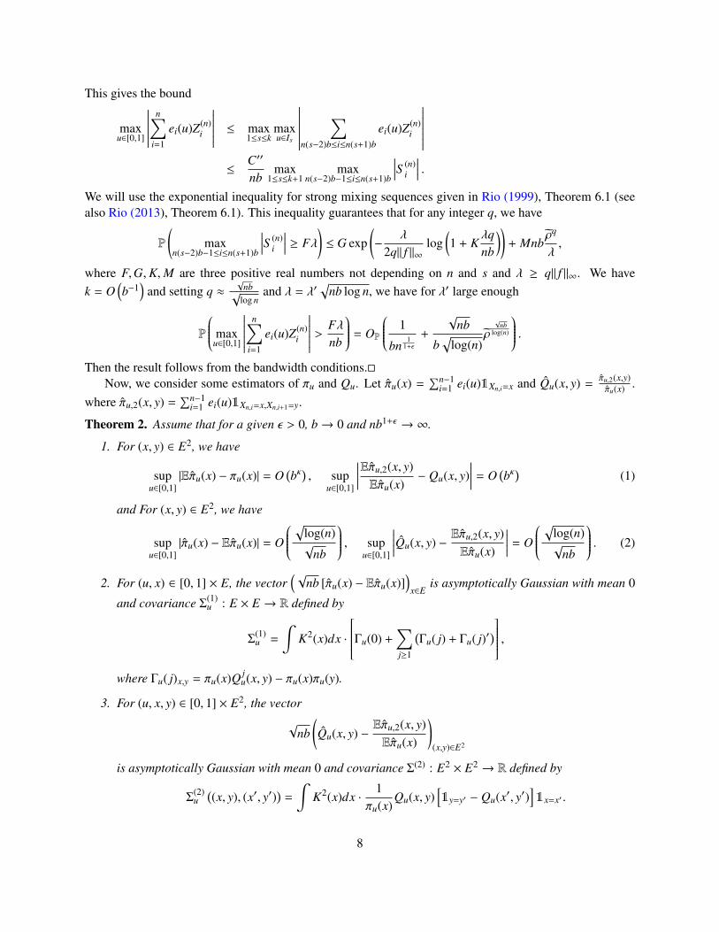
This gives the bound

maxu∈[0,1]

∣∣∣∣∣∣∣n∑

i=1

ei(u)Z(n)i

∣∣∣∣∣∣∣ ≤ max1≤s≤k

maxu∈Is

∣∣∣∣∣∣∣∣∑

n(s−2)b≤i≤n(s+1)b

ei(u)Z(n)i

∣∣∣∣∣∣∣∣≤

C′′

nbmax

1≤s≤k+1max

n(s−2)b−1≤i≤n(s+1)b

∣∣∣∣S (n)i

∣∣∣∣ .We will use the exponential inequality for strong mixing sequences given in Rio (1999), Theorem 6.1 (seealso Rio (2013), Theorem 6.1). This inequality guarantees that for any integer q, we have

P

(max

n(s−2)b−1≤i≤n(s+1)b

∣∣∣∣S (n)i

∣∣∣∣ ≥ Fλ)≤ G exp

(−

λ

2q‖ f ‖∞log

(1 + K

λqnb

))+ Mnb

ρq

λ,

where F,G,K,M are three positive real numbers not depending on n and s and λ ≥ q‖ f ‖∞. We havek = O

(b−1

)and setting q ≈

√nb√

log nand λ = λ′

√nb log n, we have for λ′ large enough

P

maxu∈[0,1]

∣∣∣∣∣∣∣n∑

i=1

ei(u)Z(n)i

∣∣∣∣∣∣∣ > Fλnb

= OP

1

bn1

1+ε

+

√nb

b√

log(n)ρ

√nb

log(n)

.Then the result follows from the bandwidth conditions.

Now, we consider some estimators of πu and Qu. Let πu(x) =∑n−1

i=1 ei(u)1Xn,i=x and Qu(x, y) =πu,2(x,y)πu(x) .

where πu,2(x, y) =∑n−1

i=1 ei(u)1Xn,i=x,Xn,i+1=y.

Theorem 2. Assume that for a given ε > 0, b→ 0 and nb1+ε → ∞.

1. For (x, y) ∈ E2, we have

supu∈[0,1]

|Eπu(x) − πu(x)| = O(bκ

), sup

u∈[0,1]

∣∣∣∣∣Eπu,2(x, y)Eπu(x)

− Qu(x, y)∣∣∣∣∣ = O

(bκ

)(1)

and For (x, y) ∈ E2, we have

supu∈[0,1]

|πu(x) − Eπu(x)| = O

√log(n)√

nb

, supu∈[0,1]

∣∣∣∣∣Qu(x, y) −Eπu,2(x, y)Eπu(x)

∣∣∣∣∣ = O

√log(n)√

nb

. (2)

2. For (u, x) ∈ [0, 1] × E, the vector(√

nb [πu(x) − Eπu(x)])

x∈Eis asymptotically Gaussian with mean 0

and covariance Σ(1)u : E × E → R defined by

Σ(1)u =

∫K2(x)dx ·

Γu(0) +∑j≥1

(Γu( j) + Γu( j)′

) ,where Γu( j)x,y = πu(x)Q j

u(x, y) − πu(x)πu(y).

3. For (u, x, y) ∈ [0, 1] × E2, the vector√

nb(Qu(x, y) −

Eπu,2(x, y)Eπu(x)

)(x,y)∈E2

is asymptotically Gaussian with mean 0 and covariance Σ(2) : E2 × E2 → R defined by

Σ(2)u

((x, y), (x′, y′)

)=

∫K2(x)dx ·

1πu(x)

Qu(x, y)[1y=y′ − Qu(x′, y′)

]1x=x′ .

8

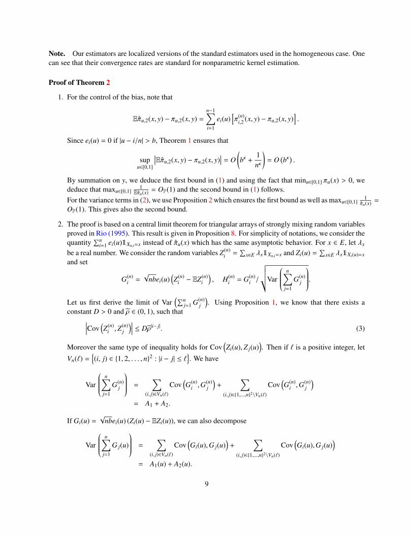
Note. Our estimators are localized versions of the standard estimators used in the homogeneous case. Onecan see that their convergence rates are standard for nonparametric kernel estimation.

Proof of Theorem 2

1. For the control of the bias, note that

Eπu,2(x, y) − πu,2(x, y) =

n−1∑i=1

ei(u)[π(n)

i,2 (x, y) − πu,2(x, y)].

Since ei(u) = 0 if |u − i/n| > b, Theorem 1 ensures that

supu∈[0,1]

∣∣∣Eπu,2(x, y) − πu,2(x, y)∣∣∣ = O

(bκ +

1nκ

)= O

(bκ

).

By summation on y, we deduce the first bound in (1) and using the fact that minu∈[0,1] πu(x) > 0, wededuce that maxu∈[0,1]

1Eπu(x) = OP(1) and the second bound in (1) follows.

For the variance terms in (2), we use Proposition 2 which ensures the first bound as well as maxu∈[0,1]1

πu(x) =

OP(1). This gives also the second bound.

2. The proof is based on a central limit theorem for triangular arrays of strongly mixing random variablesproved in Rio (1995). This result is given in Proposition 8. For simplicity of notations, we consider thequantity

∑ni=1 ei(u)1Xn,i=x instead of πu(x) which has the same asymptotic behavior. For x ∈ E, let λx

be a real number. We consider the random variables Z(n)i =

∑x∈E λx1Xn,i=x and Zi(u) =

∑x∈E λx1Xi(u)=x

and set

G(n)i =

√nbei(u)

(Z(n)

i − EZ(n)i

), H(n)

i = G(n)i /

√√√√Var

n∑j=1

G(n)j

.Let us first derive the limit of Var

(∑nj=1 G(n)

j

). Using Proposition 1, we know that there exists a

constant D > 0 and ρ ∈ (0, 1), such that∣∣∣∣Cov(Z(n)

i ,Z(n)j

)∣∣∣∣ ≤ Dρ|i− j|. (3)

Moreover the same type of inequality holds for Cov(Zi(u),Z j(u)

). Then if ` is a positive integer, let

Vn(`) =(i, j) ∈ 1, 2, . . . , n2 : |i − j| ≤ `

. We have

Var

n∑j=1

G(n)j

=∑

(i, j)∈Vn(`)

Cov(G(n)

i ,G(n)j

)+

∑(i, j)∈1,...,n2\Vn(`)

Cov(G(n)

i ,G(n)j

)= A1 + A2.

If Gi(u) =√

nbei(u) (Zi(u) − EZi(u)), we can also decompose

Var

n∑j=1

G j(u)

=∑

(i, j)∈Vn(`)

Cov(Gi(u),G j(u)

)+

∑(i, j)∈1,...,n2\Vn(`)

Cov(Gi(u),G j(u)

)= A1(u) + A2(u).

9

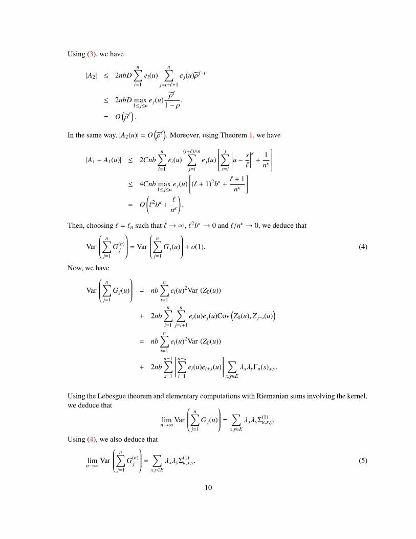
Using (3), we have

|A2| ≤ 2nbDn∑

i=1

ei(u)n∑

j=i+`+1

e j(u)ρ j−i

≤ 2nbD max1≤ j≤n

e j(u)ρ`

1 − ρ.

= O(ρ`

).

In the same way, |A2(u)| = O(ρ`

). Moreover, using Theorem 1, we have

|A1 − A1(u)| ≤ 2Cnbn∑

i=1

ei(u)(i+`)∧n∑

j=i

e j(u)

j∑s=i

∣∣∣∣∣u − s`

∣∣∣∣∣κ +1nκ

≤ 4Cnb max

1≤ j≤ne j(u)

[(` + 1)2bκ +

` + 1nκ

]= O

(`2bκ +

`

nκ

).

Then, choosing ` = `n such that ` → ∞, `2bκ → 0 and `/nκ → 0, we deduce that

Var

n∑j=1

G(n)j

= Var

n∑j=1

G j(u)

+ o(1). (4)

Now, we have

Var

n∑j=1

G j(u)

= nbn∑

i=1

ei(u)2Var (Z0(u))

+ 2nbn∑

i=1

n∑j=i+1

ei(u)e j(u)Cov(Z0(u),Z j−i(u)

)= nb

n∑i=1

ei(u)2Var (Z0(u))

+ 2nbn−1∑s=1

n−s∑i=1

ei(u)ei+s(u)

∑x,y∈E

λxλyΓu(s)x,y.

Using the Lebesgue theorem and elementary computations with Riemanian sums involving the kernel,we deduce that

limn→∞

Var

n∑j=1

G j(u)

=∑

x,y∈E

λxλyΣ(1)u,x,y.

Using (4), we also deduce that

limn→∞

Var

n∑j=1

G(n)j

=∑

x,y∈E

λxλyΣ(1)u,x,y. (5)

10

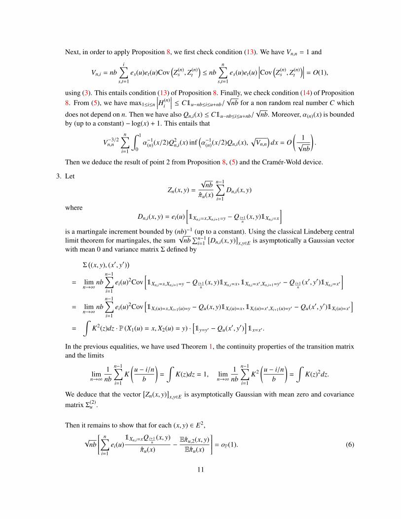
Next, in order to apply Proposition 8, we first check condition (13). We have Vn,n = 1 and

Vn,i = nbi∑

s,t=1

es(u)et(u)Cov(Z(n)

s ,Z(n)t

)≤ nb

n∑s,t=1

es(u)et(u)∣∣∣∣Cov

(Z(n)

s ,Z(n)t

)∣∣∣∣ = O(1),

using (3). This entails condition (13) of Proposition 8. Finally, we check condition (14) of Proposition8. From (5), we have max1≤i≤n

∣∣∣∣H(n)i

∣∣∣∣ ≤ C1u−nb≤i≤u+nb/√

nb for a non random real number C which

does not depend on n. Then we have also Qn,i(x) ≤ C1u−nb≤i≤u+nb/√

nb. Moreover, α(n)(x) is boundedby (up to a constant) − log(x) + 1. This entails that

V−3/2n,n

n∑i=1

∫ 1

0α−1

(n)(x/2)Q2n,i(x) inf

(α−1

(n)(x/2)Qn,i(x),√

Vn,n)

dx = O(

1√

nb

).

Then we deduce the result of point 2 from Proposition 8, (5) and the Cramér-Wold device.

3. Let

Zn(x, y) =

√nb

πu(x)

n−1∑i=1

Dn,i(x, y)

whereDn,i(x, y) = ei(u)

[1Xn,i=x,Xn,i+1=y − Q i+1

n(x, y)1Xn,i=x

]is a martingale increment bounded by (nb)−1 (up to a constant). Using the classical Lindeberg centrallimit theorem for martingales, the sum

√nb

∑n−1i=1

[Dn,i(x, y)

]x,y∈E is asymptotically a Gaussian vector

with mean 0 and variance matrix Σ defined by

Σ((x, y), (x′, y′)

)= lim

n→∞nb

n−1∑i=1

ei(u)2Cov[1Xn,i=x,Xn,i+1=y − Q i+1

n(x, y)1Xn,i=x,1Xn,i=x′,Xn,i+1=y′ − Q i+1

n(x′, y′)1Xn,i=x′

]= lim

n→∞nb

n−1∑i=1

ei(u)2Cov[1Xi(u)=x,Xi+1(u)=y − Qu(x, y)1Xi(u)=x,1Xi(u)=x′,Xi+1(u)=y′ − Qu(x′, y′)1Xi(u)=x′

]=

∫K2(z)dz · P (X1(u) = x, X2(u) = y) ·

[1y=y′ − Qu(x′, y′)

]1x=x′ .

In the previous equalities, we have used Theorem 1, the continuity properties of the transition matrixand the limits

limn→∞

1nb

n−1∑i=1

K(u − i/n

b

)=

∫K(z)dz = 1, lim

n→∞

1nb

n−1∑i=1

K2(u − i/n

b

)=

∫K(z)2dz.

We deduce that the vector[Zn(x, y)

]x,y∈E is asymptotically Gaussian with mean zero and covariance

matrix Σ(2)u .

Then it remains to show that for each (x, y) ∈ E2,

√nb

n∑i=1

ei(u)1Xn,i=xQ i+1

n(x, y)

πu(x)−Eπu,2(x, y)Eπu(x)

= oP(1). (6)

11

To show (6), we use the decomposition

√nb

n−1∑i=1

ei(u)1Xn,i=xQ i+1

n(x, y)

πu(x)−Eπu,2(x, y)Eπu(x)

=

√nb

πu(x)

n−1∑i=1

ei(u)(1Xn,i=x − π

(n)i (x)

)·

(Q i+1

n(x, y) − Qu(x, y)

)+√

nbn−1∑i=1

ei(u)π(n)i (x)

(Q i+1

n(x, y) − Qu(x, y)

)πu(x) − πu(x)πu(x)πu(x)

=An

πu(x)+ Bn

πu(x) − πu(x)πu(x)πu(x)

.

Since the kernel K has a compact support and u 7→ Qu(x, y) is κ−Hölder continuous, we have Bn =

O(√

nbbκ). Moreover, using covariance inequalities, we have Var (An) = O

(b2κ

). Then (6) follows

from πu(x) − πu(x) = OP(

1√nb

)and 1

πu(x) = OP(1). The proof of point 3 is now complete.

3 Contraction of Markov kernels using Wasserstein metrics

In this section, we consider a Polish space (E, d). For p ≥ 1, we consider the set of probability measures on(E, d) admitting a moment of order p:

Pp(E) =

µ ∈ P(E) :

∫d(x, x0)pµ(dx) < ∞

.

Here x0 is an arbitrary point in E. It is easily seen that the set Pp(E) does not depend on x0.The Wasserstein metric Wp of order p associated to d is defined by

Wp(µ, ν) = infγ∈Γ(µ,ν)

∫E×E

d(x, y)pdγ(x, y)1/p

where Γ(µ, ν) denotes the collection of all probability measures on E × E with marginals µ and ν. We willsay that γ ∈ Γ(µ, ν) is an optimal coupling of (µ, ν) if(∫

d(x, y)pγ(dx, dy))1/p

= Wp(µ, ν).

It is well-known that an optimal coupling always exist. See Villani (2009) for some properties of Wassersteinmetrics.

In the sequel, we will use the following assumptions.

B1 For all (u, x) ∈ [0, 1] × E, δxQu ∈ Pp(E).

B2 There exist a positive integer m and two real numbers r ∈ (0, 1) and C1 ≥ 1 such that for all u ∈ [0, 1]and all x ∈ E,

Wp(δxQm

u , δyQmu

)≤ rd(x, y), Wp

(δxQu, δyQu

)≤ C1d(x, y).

B3 The family of transitions Qu : u ∈ [0, 1] satisfies the following Hölder type continuity condition. Thereexist κ ∈ (0, 1] and C2 > 0, such that for all x ∈ E and all u, v ∈ [0, 1],

Wp (δxQu, δxQv) ≤ C2 (1 + d(x, x0)) |u − v|κ.

12

Note. If R is a Markov kernel, the Dobrushin contraction coefficient is now defined by

c(R) = sup(x,y)∈E2

x,y

Wp(δxR, δyR

)d(x, y)

.

Thus Assumption B2 means that supu∈[0,1] c (Qu) < ∞ and supu∈[0,1] c(Qm

u)< 1.

The following proposition shows that under these assumptions, the marginal distribution of the Markovchain with transition Qu converges exponentially fast to its unique invariant probability distribution whichis in turn Hölder continuous with respect to u, in Wasserstein metric.

Proposition 3. Assume that assumptions B1-B3 hold true and set for an integer j ≥ 1,

1. For all u ∈ [0, 1], the Markov chain of transition Qu has a unique invariant probability distributiondenoted by πu. Moreover for all initial probability distribution µ ∈ Pp(E), we have for n = m j + s

Wp(µQn

u, πu)≤ Cs

1r j

(∫ d(x, x0)pµ(dx))1/p

+ κ2

,where κ2 = supu∈[0,1]

(∫d(x, x0)pπu(dx)

)1/p.

2. If u, v ∈ [0, 1], we have

Wp(πu, πv) ≤C2|u − v|κ

1 − r

mCm−11 κ2 +

m−1∑j=0

C j1κ1(m − j − 1)

,where κ1( j) = supu∈[0,1]

(∫d(x, x0)pQ j

u(x0, dx))1/p

.

Proof of Proposition 3 We first show that the quantities κ1( j) are finite. We set q j =(∫

(1 + d(x, x0))p Q j0(x0, dx)

)1/p.

If j ≥ 1, we have, using Lemma 1,

Wp(δx0 Q j

u, δx0 Q j0

)≤ Wp

(δx0 Q j

u, δx0 Q j−10 Qu

)+ Wp

(δx0 Q j−1

0 Qu, δx0 Q j0

)= C1Wp

(δx0 Q j−1

u , δx0 Q j−10

)+ C2|u|κq j−1.

Then we obtain

Wp(δx0 Q j

u, δx0 Q j0

)≤ C2

j−1∑s=0

Cs1q j−s−1. (7)

Then, using Lemma 3 for the function f (x) = 1 + d(x, x0), we get

κ1( j) ≤ q j + C2

j−1∑s=0

Cs1q j−s−1.

13

1. The existence and unicity of an invariant probability πu ∈ Pp easily follows from the fixed pointtheorem for a contractant application in the complete metric space

(Pp,Wp

).

Before proving the geometric convergence, let us show that the quantity κ2 is finite. We have, usingLemma 1,

Wp(πu, π0) ≤ Wp(πuQm

u , π0Qmu)

+ Wp(π0Qm

u , π0Qm0

)≤ rWp (πu, π0) +

(∫W p

p

(δxQm

u , δxQm0

)π0(dx)

)1/p

.

Using (7) and Lemma (1), we have

Wp(δxQm

u , δxQm0

)≤ Wp

(δxQm

u , δx0 Qmu)

+ Wp(δx0 Qm

u , δx0 Qm0

)+ Wp

(δxQm

0 , δx0 Qm0

)≤ 2rd(x, x0) + C2

m−1∑s=0

C j1qm−s−1.

From the previous bound, we easily deduce the existence of a real number D > 0, not depending onu, such that Wp(πu, π0) ≤ D

1−r . Then, using Lemma 3, we get

κ2 ≤D

1 − r+

(∫d(x, x0)pπ0(dx)

)1/p

,

which is finite.Now, the geometric convergence is a consequence of the inequality

Wp(µQn

u, πuQnu)≤ Cs

1r jWp(µ, πu) ≤ Cs1r j

(∫ d(x, x0)pµ(dx))1/p

+ κ2

.Finally, let ν be an invariant probability for Pu (not necessarily in Pp). Let f : E → R be an elementof Cb(E). Since convergence in Wasserstein metric implies weak convergence, we have from thegeometric ergodicity limn→∞ Qn

u f (x) = πu f for all x ∈ E. Hence, using the Lebesgue theorem, wehave

ν f = νQnu f =

∫ν(dx)Qn

u f (x)→ πu f

which shows the unicity of the invariant measure.

2. Proceeding as for the previous point, we have

Wp(πu, πv) ≤ rWp(πu, πv) +

(∫W p

p(δxQm

u , δxQmv)πv(dx)

)1/p

. (8)

But

Wp(δxQm

u , δxQmv)≤ C1Wp

(δxQm−1

u , δxQm−1v

)+ C2|u − v|κ

(∫ [1 + d(y, x0)

]p Qm−1v (x, dy)

)1/p

≤ C1Wp(δxQm−1

u , δxQm−1v

)+ C2|u − v|κ

(κ1(m − 1) + Cm−1

1 d(x, x0)).

14

We deduce that

Wp(δxQm

u , δxQmv)≤ C2|u − v|κ

m−1∑j=0

C j1κ1(m − j − 1) + mCm−1

1 d(x, x0)

.Reporting the last bound in (8), we get the result.

Now let us give the main result of this section. For j ∈ N∗, we endow the space E j with the distance

d j(x, y) =

j∑s=1

d(xs, ys)p

1/p

, x, y ∈ E j.

We will still denote by Wp the Wasserstein metric for Borelian measures on E j.

Theorem 3. Assume that assumptions B1 − B3 hold true. Then the triangular array of Markov chainsXn,k : n ∈ Z+, k ≤ n

is locally stationary. Moreover, there exists a real number C > 0, only depending on

j, p, d, κ, r,C1,C2, κ1(1), . . . , κ1(m), κ2 such that

Wp(π(n)

k, j, πu, j)≤ C

k+ j−1∑s=k

∣∣∣∣∣u − sn

∣∣∣∣∣κ +1nκ

.Proof of Theorem 3

1. We show the result by induction and first consider the case j = 1. For k ≤ n, let Qk,m be the probabilitykernel Q k−m+1

n· · ·Q k

n. We have

Wp(π(n)

k , πu)

= Wp(π(n)

k−mQk,m, πuQmu

)≤ Wp

(π(n)

k−mQk,m, π(n)k−mQm

u

)+ Wp

(π(n)

k−mQmu , πuQm

u

)≤ rWp

(π(n)

k−m, πu)

+

(∫W p

p(δxQk,m, δxQm

u)π(n)

k−m(dx))1/p

.

From Lemma 2, we have

Wp(δxQk,m, δxQm

u)≤

m−1∑s=0

Cs1C2

[∫(1 + d(y, x0))p δxQ k−m+1

n· · ·Q k−s−1

n(dy)

]1/p ∣∣∣∣∣u − k − sn

∣∣∣∣∣κ .First we note that from our assumptions and using Lemma 3 for the function f (x) = 1 + d(x, x0), wehave [

δxQu f p]1/p≤

[δx0 Qu f p]1/p

+ C1d(x, x0) ≤ (1 + κ1(1) + C1) f (x),

where κ1 is defined in Proposition 3. Then we get supu∈[0,1] δxQu f p ≤ Cp3 f p(x), where C3 = 1 +

κ1(1) + C1. This yields to the inequality

Wp(δxQk,m, δxQm

u)≤

m−1∑s=0

Cs1C2Cm−s−1

3

∣∣∣∣∣u − k − sn

∣∣∣∣∣κ f (x).

15

Then we obtain

Wp(π(n)

k , πu)≤ rWp

(π(n)

k−m, πu)

+

m−1∑s=0

Cs1C2Cm−s−1

3

∣∣∣∣∣u − k − sn

∣∣∣∣∣κ (π(n)k−m f p

)1/p.

Then the result will easily follow if we prove that supn,k≤n π(n)k f p < ∞. Setting ck = Wp

(π(n)

k , π kn

)and

C4 =∑m−1

s=0 (s + 1)κCs+11 C2Cm−s−1

3 and using our previous inequality, we have

ck ≤ rWp

(π(n)

k−m, π kn

)+

C4

nκ(π(n)

k−m f p)1/p

≤

(r +

C4

nκ

)ck−m + rWp

(π k−m

n, π k

n

)+

C4

nκ(1 + κ2).

Then, if n0 is such that for all n ≥ n0, r +C4nκ < 1, the last inequality, Proposition 3 and Lemma

3 guarantee that supn≥n0,k≤n π(n)k f p is finite and only depends on p, d, r,C1,C2, κ1(1), . . . , κ1(m), κ2, κ.

Moreover if n ≤ n0, we have(π(n)

k f p)1/p≤ (C4 + 1)n0 (π0 f p)1/p. This concludes the proof for the case

j = 1.

2. Now for j ≥ 2, we define a coupling of(π(n)

k, j, πu, j)

as follows. First we consider an optimal cou-

pling Γ(k,n)u, j−1 of

(π(n)

k, j−1, πu, j−1), and for each (x, y) ∈ E2, we define an optimal coupling ∆

(k,n)x,y, j,u of(

δxQ k+ jn, δyQu

). From Villani (2009), Corollary 5.22, it is possible to choose this optimal coupling

such that the application (x, y) 7→ ∆(k,n)x,y, j,u is measurable. Now we define

Γ(k,n)u, j (dx1, dy1, . . . , dx j, dy j) = ∆

(k,n)x j−1,y j−1, j,u

(dx j, dy j)Γ(k,n)u, j−1(dx1, dy1, . . . , dx j−1, dy j−1).

Then we easily deduce that

W pp

(π(n)

k, j, πu, j)≤ W p

p

(π(n)

k, j−1, πu, j−1)

+

∫W p

p

(δx j−1 Q k+ j

n, δy j−1 Qu

)Γ

(n,k)u, j−1

(dx1, dy1, . . . , dx j−1, dy j−1

).

SinceWp

(δx j−1 Q k+ j

n, δy j−1 Qu

)≤ C1d(x j−1, y j−1) + C2

[1 + d(y j−1, x0)

] ∣∣∣∣∣u − k + jn

∣∣∣∣∣κ .This leads to

Wp(π(n)

k, j, πu, j)≤ (1 + C1)Wp

(π(n)

k, j−1, πu, j−1)

+ C2(1 + κ2)∣∣∣∣∣u − k + j

n

∣∣∣∣∣κ .The results follows by a finite induction.

Finally, note that Condition 1 of Definition 1 follows from induction and the point 2 of Proposition 3,because using the same type of arguments, we have

Wp(πv, j, πu, j

)≤ (1 + C1)Wp

(πv, j−1, πu, j−1

)+ C2(1 + κ2) |u − v|κ .

The proof of the Theorem is now complete.

16

3.1 Mixing conditions

We now introduce another useful coefficient: the τ−mixing coefficient introduced and studied in Dedeckerand Prieur (2004) that we will adapt to our triangular arrays. This coefficient has been introduced for Banachspaces E. In the sequel, we denote by Λ1(E) the set of 1−Lipschitz functions from E to R. Assume first thatE = R and as for the β−mixing coefficients, set Xn, j = 0 for j > n. Then setting

U(F

(n)i , Xn,i+ j

)= sup

∣∣∣∣E [f(Xn,i+ j|F

(n)i

)]− E

[f(Xn,i+ j

)]∣∣∣∣ : f ∈ Λ1(R),

the τn−mixing coefficient for the sequence(X(n)

j

)j∈Z

is defined by

τn( j) = supi∈ZE

[U

(F

(n)i , Xn,i+ j

)].

Now for a general metric space E, the τn−mixing coefficient is defined by

τn( j) = supf∈∆1(E)

supi∈ZE

[U

(F

(n)i , f

(Xn,i+ j

))].

Note that, if Xn,i denotes a copy of Xn,i,

τn( j) ≤ supi∈ZEd

(Xn,i, Xn,i

),

For bounding this mixing coefficient, the following assumption, which strengthens assumption B2 in thecase m ≥ 2 and p = 1, will be needed.

B4 There exists a positive real number ε such that for all (u, u1, . . . , um) ∈ [0, 1]m+1 satisfying |ui − u| < ε

for 1 ≤ i ≤ m, we haveW1

(δxQu1 · · ·Qum , δyQu1 · · ·Qum

)≤ rd(x, y),

where m and r are defined in assumption B2.

Proposition 4. Assume that assumptions B2 and B4 hold true. Then there exists C > 0 and ρ ∈ (0, 1), onlydepending on m, r,C1, ε such that

τn( j) ≤ Cρ j.

Proof of Proposition 4 We first consider the case n ≥ m/ε. Now if k is an integer such that k + m− 1 ≤ n,note that assumption B4 entails that

W1

(µQ k

n· · ·Q k+m−1

n, νQ k

n· · ·Q k+m−1

n

)≤ rW1(µ, ν), (9)

where the probability measures µ and ν have both a finite first moment. If j = mt + s, we get from (9) andAssumption B2,

τn( j) ≤ Cs1rt sup

i∈ZE

[W1

(δXn,i , π

(n)i

)]≤ 2 sup

i∈ZEd

(Xn,i, x0

)·Cs

1rt.

We have seen in the proof of Theorem 3 that supn∈Z,i≤n Ed(Xn,i, x0

)< ∞.

Now assume that n < m/ε. If j ≤ n, we have

τn( j) ≤ 2 supi∈ZEd

(Xn,i, x0

)·Cm/ε

1 .

Now if j > n, we have since (Xn, j) j≤0 is stationary with transition kernel Q0,

τn( j) ≤ 2 supi∈ZEd

(Xn,i, x0

)·Cm/ε+m

1 r[ j−n

m

].

This leads to the result for ρ = r1/m and an appropriate choice of C > 0.

17

Note. Let us remind that Proposition 4 implies a geometric decrease for the covariances. This is a conse-quence of the following property. If f : E → R is measurable and bounded and g : E → R is measurableand Lipschitz, we have

Cov(

f(Xn,i

), g

(Xn,i+ j

))≤ ‖ f ‖∞ · δ(g) · τn( j).

3.2 An extension to q−order Markov chains

We start with an extension of our result to Markov sequences of order q ≥ 1 and taking values in the Polishspace (E, d). Let S u : u ∈ [0, 1] be a family of probability kernels from (Eq,B(Eq)) to (E,B(E)). The twofollowing assumptions will be used.

H1 For all x ∈ Eq, S u(x, ·) ∈ Pp(E).

H2 There exist non-negative real numbers a1, a2, . . . , aq satisfying∑q

j=1 a j < 1 and such that for all (u, x, y) ∈[0, 1] × Eq × Eq,

Wp (S u(x, ·), S u(y, ·)) ≤q∑

j=1

a jd(x j, y j).

H2 There exists a positive real number C and κ ∈ (0, 1) such that for all (u, , v, x) ∈ [0, 1] × [0, 1] × Eq,

Wp (S u(x, ·), S v(x, ·)) ≤ C

1 +

q∑j=1

d(x j, x0)

|u − v|κ.

To define Markov chains, we consider the family of Markov kernels Qu : u ∈ [0, 1] on the measurablespace (Eq,B(E)q) and defined by

Qu (x, dy) = S u(x, dyq

)⊗ δx2(y1) ⊗ · · · ⊗ δxq(dyq−1).

Corollary 2. If the assumptions H1-H3 hold true then Theorem 3 and Proposition 4 apply.

Proof of Corollary 10 Assumption H1 entails B1. Then we check assumption B3. If (u, v, x) ∈ [0, 1] ×[0, 1] × Eq, let αx,u,v be a coupling of the two probability distributions S u(x, ·) and S v(x, ·). Then

γx,u,v(dy, dy′) = αx,u,v(dyq, dy′q) ⊗q−1j=1 δx j+1(dy j) ⊗ δx j+1(dy′j)

defines a coupling of the two measures δxQu and δxQv. We have

Wp (δxQu, δxQv) ≤[∫

d(yq, y′q)pαx,u,v(dyq, dy′q)]1/p

.

By taking the infinimum of the last bound over all the couplings, we get

Wp (δxQu, δxQv) ≤ Wp (S u (x, ·) , S v (x, ·)) ,

which shows B3, using assumption H3.Finally, we check assumptions B2 and B4. For an integer m ≥ 1, (u1, . . . , um) ∈ [0, 1]m and (x, y) ∈ Eq × Eq,

18

we denote by αx,y,u an optimal coupling of (S u(x, ·), S u(y, ·)). From Villani (2009), Corollary 5.22, thereexists a measurable choice of (x, y) 7→ αxy,u. We define

γ(xq+1yq+1)m,u1,...,um

(dxq+1, . . . , dxq+m, dyq+1, . . . , dyq+m

)=

q+m∏i=q+1

αxi,yi,ui(dxi, dyi),

where xi = (xi−1, . . . , xi−q). Let Ω = Em×Em endowed with its Borel sigma field and the probability measureP = γ

(xq+1yq+1)m,u1,...,um . Then we define the random variables Zxq+1

j = x j, Zyq+1j = y j for 1 ≤ j ≤ q and for 1 ≤ j ≤ m,

Zxq+1q+ j (ω1, ω2) = ω1, j, Zyq+1

q+ j (ω1, ω2) = ω2, j for j = 1, . . . ,m. By definition of our couplings, we have

E1/p[d(Zxq+1

k ,Zyq+1k

)p]≤

q∑j=1

a jE1/p

[d(Zxq+1

k− j ,Zyq+1k− j

)p].

Using a finite induction, we obtain

E1/p[d(Zxq+1

k ,Zyq+1k

)p]≤ α

kq max

1≤ j≤qd(x j, y j),

where α =∑q

j=1 a j. Setting Xxm =

(Zx

m−q+1, . . . ,Zxm

), this entails

Wp(δxQu1 · · ·Qum , δyQu1 · · ·Qum

)≤ E1/p

[dq

(Xx

m, Xym

)p]≤

q∑j=1

αm− j+1

q max1≤ j≤q

d(x j, y j)

≤

q∑j=1

αm− j+1

q · dq(x, y).

Then B2-B4 are satisfied if m is large enough by noticing that W1 ≤ Wp.

3.3 Examples of locally stationary Markov chains

Natural examples of a q−order Markov chain satisfying the previous assumptions are based on time-varyingautoregressive process. More precisely, if E and G are measurable spaces and F : [0, 1] × Eq ×G → E, thetriangular array

Xn,i : i ≤ n, n ∈ Z+ is defined recursively by the equations

Xn,i = F( in, Xn,i−1, . . . , Xn,i−q, εi

), i ≤ n, (10)

where the usual convention is to assume that

Xn,i = F(0, Xn,i−1, . . . , Xn,i−q, εi

), i ≤ 0.

Then, if S u(x, ·) denotes the distribution of F(u, xq, . . . , x1, ε1

), we have

Wp (S u(x, ·), S u(y, ·)) ≤ E1/p[d(F

(u, xq, . . . , x1, ε1

), F

(u, yq, . . . , y1, ε1

))p],

Wp (S u(x, ·), S v(x, ·)) ≤ E1/p[d(F

(u, xq, . . . , x1, ε1

), F

(v, xq, . . . , x1, ε1

))p].

19

Then the assumptions H1 −H3 are satisfied if for all (u, v, x, y) ∈ [0, 1] × [0, 1] × Eq × Eq,

E1/p[d(F(u, xq, . . . , x1), x0

)p]< ∞,

E1/p[d(F(u, xq, . . . , x1), F(u, yq, . . . , y1)

)p]≤

q∑j=1

a jd(xq− j+1, yq− j+1

)and

E1/p[d(F(u, xq, . . . , x1), F(v, xq, . . . , x1)

)p]≤ C

1 +

q∑j=1

d(x j, x0)

· |u − v|κ.

A typical example of such time-varying autoregressive process is the univariate tv-ARCH process for which

Xn,i = ξi

√√√a0(i/n) +

q∑j=1

a j(i/n)X2n,i− j,

with Eξt = 0, Var ξt = 1. The previous assumptions are satisfied for the square of this process if the a j’s areκ−Hölder continuous and if

‖ξ2t ‖p · sup

u∈[0,1]

q∑j=1

a j(u) < 1, for some p ≥ 1.

See Fryzlewicz et al. (2008) and Truquet (2016) for the use of those processes for modeling financial data.

Note. The approximation of time-varying autoregressive processes by stationnary processes is discussedin several papers. See for instance Subba Rao (2006) for linear autoregressions with time varying randomcoefficients, Vogt (2012) for nonlinear time-varying autoregressions or Zhang and Wu (2015) for additionalresults in the same setting. However, the approximating stationary process of (10) is given by

Xi(u) = F(u, Xi−1(u), . . . , Xi−q(u), εi

).

Note that Wp(π(n)

k , πu)≤ E1/p

[d(X(n)

k , Xk(u))p]

and the aforementioned references usually study a controlof this upper bound by

∣∣∣u − kn

∣∣∣κ + 1nκ . Note that in the case of autoregressive processes, a coupling of the

time-varying processes and its stationary approximation is already defined because the same noise pro-cess is used in both cases. However it is possible to construct some examples for which π(n)

k = πu andE1/p [

d(Xn,k, Xk(u)

)p] , 0, i.e the coupling used is not optimal. Nevertheless, it is still possible to obtainan upper bound of E1/p

[d(X(n)

k , Xk(u))p]

using our results. To this end, let us assume that q = 1 (otherwiseone can use vectors of q−successive coordinates to obtain a Markov chain of order 1) if u ∈ [0, 1], and weconsider the Markov kernel form

(E2,B(E2)

)to itself, given by

Q(u)v (x1, x2, A) = P ((F(v, x1, ε1), F(u, x2, ε1)) ∈ A) , A ∈ B(E2), v ∈ [0, 1].

One can show that the familyQ(u)

v : v ∈ [0, 1]

satisfies the assumptions B1 − B4 for the metric

d2[(x1, x2), (y1, y2)

]=

(d(x1, y1)p + d(x2, y2)p)1/p .

Moreover, the constant in Theorem 3 does not depend on u ∈ [0, 1]. Then Lemma 4 guarantees that thereexists a positive constant C not depending on k, n, u such that

E1/p (d(Xk,n, Xk(u)

)p)≤ C

[∣∣∣∣∣u − kn

∣∣∣∣∣κ +1nκ

].

20

Iteration of random affine functions Here we assume that for each u ∈ [0, 1], there exists a sequence(At(u), Bt(u))t∈Z of i.i.d random variables such that At(u) takes its values in the spaceMd of squares matricesof dimension d with real coefficients and Bt(u) takes its values in E = Rd. Let ‖ · ‖ a norm on E. We alsodenote by ‖ · ‖ the corresponding operator norm onMd. We then consider the following recursive equations

Xn,i = Ai

( in

)Xn,i−1 + Bi

( in

). (11)

Local approximation of these autoregressive processes by their stationary versions Xt(u) = At(u)Xt−1(u) +

Bt(u) is studied is studied by Subba Rao (2006). In this subsection, we will derive similar results using ourMarkov chain approach. For each u ∈ [0, 1], we denote by γu the top Lyapunov exponent of the sequence(At(u))t∈Z, i.e

γu = infn≥1

1nE log ‖An(u)An−1(u) · · · A1(u)‖.

We assume that there exists t ∈ (0, 1) such that

R1 for all u ∈ [0, 1], E‖A1(u)‖t < ∞, E‖B1(u)‖t < ∞ and γu < 0.

R2 There exists C > 0 and κ ∈ (0, 1) such that for all (u, v) ∈ [0, 1]2,

E‖A1(u) − A1(v)‖t + E‖B1(u) − B1(v)‖t ≤ C|u − v|tκ.

Proposition 5. For s ∈ (0, 1), we set d(x, y) = ‖x − y‖s. Assume that assumptions R1 − R2 hold true. Thenthere exists s ∈ (0, t) such that Theorem 3 applies with p = 1, κ = tκ and d(x, y) = ‖x − y‖s and x0 = 0.

Notes

1. Using the remark in the Note of Section 3.3, we also have E‖Xn,k−Xk(u)‖s ≤ C(∣∣∣u − k

n

∣∣∣κ + 1nκ

)s, where

the process(X j(u)

)j∈Z

satisfies the iterations Xk(u) = Ak(u)Xk−1(u) + Bk(u). Then the triangular arrayXn,k : k ≤ n, n ∈ Z+ is locally stationary in the sense given in Vogt (2012) (see Definition 2.1 of that

paper).

2. One can also give additional results for the Wasserstein metric of order p ≥ 1 and d(x, y) = ‖x − y‖ if

E‖A1(u)‖p + E‖B1(u)‖p < ∞, E1/p‖A1(u) − A1(v)‖p + E1/p‖B1(u) − B1(v)‖p ≤ C|u − v|κ

and there exists an integer m ≥ 1 such that supu∈[0,1] E‖Am(u) · · · A1(u)‖p < 1. In particular, one canrecover results about the local approximation of tv-AR processes defined by

Xn,i =

q∑j=1

a j(i/n)Xn,i− j + σ(i/n)εi

by vectorizing q successive coordinates and assuming κ−Hölder continuity for the a j’s and σ. Detailsare omitted.

21

Proof of Proposition 5 For all (x, u) ∈ Rd × [0, 1], the measure δxQu is the probability distribution of therandom variable Ak(u)x+Bk(u). Condition A1 of Theorem 3 follows directly from assumption R1 (whateverthe value of s ∈ (0, t)). Moreover, we have for s ∈ (0, t),

W1 (δxQu, δxQv) ≤ E‖Ak(u) − Ak(v)‖s · ‖x‖s + E‖Bk(u) − Bk(v)‖s

≤(1 + ‖x‖s

)·(E

st ‖Ak(u) − Ak(v)‖t + E

st ‖Bk(u) − Bk(v)‖t

).

This entails condition A3, using assumption R2. Next, if u ∈ [0, 1], the conditions γu < 0 and E‖At(u)‖t < ∞entail the existence of an integer ku and su ∈ (0, t) such that E‖Aku(u)Aku−1(u) · · · A1(u)‖su < 1 (see forinstance Francq and Zakoïan (2010), Lemma 2.3). Using the axiom of choice, let us select for each u, acouple (ku, su) satisfying the previous property. From assumption R2, the set

Ou =v ∈ [0, 1] : E‖Aku(v)Aku−1(v) · · · A1(v)‖su < 1

is an open set of [0, 1]. By a compactness argument, there exist u1, . . . , ud ∈ [0, 1] such that [0, 1] = ∪d

i=1Oui .Then setting s = min1≤i≤d sui and denoting by m the lowest common multiple of the integers ku1 , . . . , kud , wehave from assumption R2,

r = supu∈[0,1]

E‖Am(u) · · · A1(u)‖s < 1.

This entails condition B2 for this choice of s, m and r. Indeed, we have

W1(δxQm

u , δyQmu

)≤ E‖Am(u) · · · A1(u)(x − y)‖s ≤ rd(x, y).

Note also that condition B4 easily follows from the uniform continuity of the application (u1, . . . , um) 7→E‖Am(u1) · · · A1(um)‖s ..

Time-varying integer-valued autoregressive processes (tv-INAR) Stationary INAR processes are widelyused in the time series community. This time series model has been proposed by Al Osh and Alzaid (1987)and a generalization to several lags was studied in Jin-Guan and Yuan (1991). In this paper, we introduce alocally stationary version of such processes. For u ∈ [0, 1] and j = 1, 2, . . . , q + 1, we consider a probabilityζ j(u) on the nonnegative integers and for 1 ≤ j ≤ q, we denote by α j(u) the mean of the distribution ζ j(u).Now let

Xn,k =

q∑j=1

Xn,k− j∑i=1

Y (n,k)j,i + η(n)

k ,

where for each integer n ≥ 1, the familyY (n,k)

j,i , η(n)h : (k, j, i, h) ∈ Z4

contains independent random vari-

ables and such that for 1 ≤ j ≤ q, Y (n,k)j,i has probability distribution ζ j(k/n) and η(n)

k has probabilitydistribution ζq+1(k/n). Note that, one can define a corresponding stationary autoregressive process. Tothis end, we denote by F j,u the cumulative distribution of the probability ζ j(u) and we consider a fam-ily

U(k)

j,i ,Vk : (i, j, k) ∈ Z3

of i.i.d random variables uniformly distributed over [0, 1] and we set Y (n,k)j,i =

F−1j,k/n

(U(k)

j,i

)where for a cumulative distribution function G, G−1 denotes its left continuous inverse. Then

one can consider the stationary version

Xk(u) =

q∑j=1

Xk− j(u)∑i=1

F−1j,u

(U(k)

j,i

)+ F−1

q+1,u (Vk) .

The following result is a consequence of Corollary 10. Only the case p = 1 is considered here.

22

Corollary 3. Let d be the usual distance on R. Assume that supu∈[0,1]∑q

j=1 α j(u) < 1, ζq+1 has a finite first

moment and W1(ζ j(u), ζ j(v)

)≤ C|u − v|κ for C > 0, κ ∈ (0, 1) and 1 ≤ j ≤ q + 1. Then Theorem 3 and

Proposition 4 apply.

Example. Stationary INAR processes are often used when ζ j is a Bernoulli distribution of parameterα j ∈ (0, 1) for 1 ≤ j ≤ q and ζq+1 is a Poisson distribution of parameter λ. This property guarantees thatthe marginal distribution is also Poissonian. Condition

∑qj=1 α j < 1 is a classical condition ensuring the

existence of a stationary solution for this model. In the locally stationnary case, let U be a random variablefollowing a uniform distribution over [0, 1] and (Nt)t be a Poisson process of intensity 1. Then, we have

W1(ζ j(u), ζ j(v)

)≤ E

∣∣∣1U≤α j(u) − 1U≤α j(v)∣∣∣ ≤ ∣∣∣α j(u) − α j(v)

∣∣∣ ,W1

(ζq+1(u), ζq+1(v)

)≤ E

∣∣∣Nλ(u) − Nλ(v)∣∣∣ ≤ |λ(u) − λ(v)| .

Then the assumptions of Corollary 3 are satisfied if the functions α j and λ are κ−Hölder continuous and if∑qj=1 α j(u) < 1, u ∈ [0, 1].

Note. One can also state a result for p ≥ 1. This case is important if we have to compare the expectationof some polynomials of the time-varying process with its the stationary version. However, in the examplegiven above, a naive application of our results will require

∑qj=1 α j(u)1/p < 1. Moreover, one can show that a

κ−Hölder regularity on α j and λ entails a κp−Hölder regularity in Wasserstein metrics. For instance if q = 1,

we have Wp (δ0Qu, δ0Qv) ≥ |λ(u) − λ(v)|1/p. In order to avoid these unnatural conditions for this model, wewill use the approach developed in Section 4.

4 Local stationarity and drift conditions

In this section, we will use some drift and minoration conditions to extend the Dobrushin’s contractiontechnique of Section 2. A key result for this section is Lemma 5 which is adapted from Lemma 6.29 inDouk et al. (2014). This result gives sufficient conditions for contracting Markov kernels with respect tonorm induced by a particular Foster-Lyapunov drift function. The original argument for such contractionproperties is due to Hairer and Mattingly (2011). This important result will enable us to consider additionalexamples of locally stationary Markov chains with non compact state spaces. For a function V : E → [1,∞),we define the V−norm of signed measure µ on (E,B(E)) by

‖µ‖V = supf :| f (x)|≤V(x)

∣∣∣∣∣∫ f dµ∣∣∣∣∣ . (12)

4.1 General result

We will assume that there exists a measurable function V : E → [1,∞) such that

F1 there exist ε > 0, λ ∈ (0, 1), an integer m ≥ 1 and two real numbers b > 0,K ≥ 1 such that for allu, u1, . . . , um ∈ [0, 1] satisfying |u − ui| ≤ ε,

QuV ≤ KV, Qu1 · · ·QumV ≤ λV + b.

Moreover, there exists η > 0, R > 2b/(1 − λ) and a probability measure ν ∈ P(E) such that

δxQu1 · · ·Qum ≥ ην, if V(x) ≤ R,

23

F2 there exist κ ∈ (0, 1) and a function V : E → (0,∞) such that supu∈[0,1] πuV < ∞ and for all x ∈ E,‖δxQu − δxQv‖V ≤ V(x)|u − v|κ.

We first give some properties of the Markov kernels Qu with respect to the V−norm.

Proposition 6. Assume that assumptions F1 − F2 hold true.

1. There exist C > 0 and ρ ∈ (0, 1) such that for all x ∈ E,

supu∈[0,1]

‖δxQ ju − πu‖V ≤ CV(x)ρ j.

Moreover supu∈[0,1] πuV < ∞.

2. There exists C > 0 such that for all (u, v) ∈ [0, 1]2,

‖πu − πv‖V ≤ C |u − v|κ .

Proof of Proposition 6.

1. According to Lemma 5, there exists (γ, δ) ∈ (0, 1)2 only depending λ, b, η, such that

∆Vδ(Qmu ) = sup

‖µR − νR‖Vδ‖µ − ν‖Vδ

: µ, ν ∈ P(E), µVδ < ∞, νVδ < ∞≤ γ,

with Vδ = 1−δ+δV . From Theorem 6.19 in Douk et al. (2014) and Assumption F1, we have a uniqueinvariant probability for Qu, satisfying πuV < ∞ and for µ ∈ P(E) such that µV < ∞, we have

‖µQ ju − πu‖Vδ ≤ max

0≤s≤m−1∆Vδ(Q

su)γ[ j/m]‖µ − πu‖Vδ .

Note that ‖ · ‖Vδ ≤ ‖ · ‖V ≤1δ ‖ · ‖Vδ and the two norms are equivalent. Using Lemma 6.18 in Douk et al.

(2014), we have

∆Vδ(Qsu) = sup

x,y

‖δxQsu − δyQs

u‖Vδ

Vδ(x) + Vδ(y)≤

K s

δ.

Then it remains to show that supu∈[0,1] πuV < ∞ or equivalently supu∈[0,1] πuVδ < ∞. But this aconsequence of the contraction property of the application µ 7→ µQm

u on the space

Mδ = µ ∈ P(E) : µVδ < ∞

endowed with the distance dδ(µ, ν) = ‖µ − ν‖Vδ , which is a complete metric space (see Proposition6.16 in Douk et al. (2014)). Hence we have

µ − πu =

∞∑j=0

[µQm j

u − µQm( j+1)u

]which defines a normally convergent series inMδ and

‖µ − πu‖Vδ ≤

∞∑j=0

γ j‖µ − µQmu ‖Vδ ≤

µV + KmµV1 − γ

.

This shows that supu∈[0,1] πuV < ∞ and the proof of the first point is now complete.

24

2. To prove the second point, we decompose as in the two previous sections πu − πv = πuQmu − πvQm

u +

πvQmu − πvQm

v . This leads to the inequality

‖πu − πv‖Vδ ≤‖πvQm

u − πvQmv ‖Vδ

1 − γ.

Moreover, we have

‖πvQmu − πvQm

v ‖Vδ ≤ ‖πvQmu − πvQm

v ‖V

≤

m−1∑j=0

‖πvQm− j−1v (Qv − Qu)Q j

u‖V

≤

m−1∑j=0

K j‖πvQm− j−1v (Qv − Qu)‖V

≤

m−1∑j=0

K j · πvV · |u − v|κ.

Hence the result follows with C =supu∈[0,1] πuV

1−γ∑m−1

j=0 K j.

Now, we give our result about local stationarity.

Theorem 4. 1. Under the assumptions F1 − F2, there exists a positive real number C, only dependingon m, λ, b,K and supu∈[0,1] πuV such that

‖π(n)k − πu‖V ≤ C

[∣∣∣∣∣u − kn

∣∣∣∣∣κ +1nκ

].

2. Assume that assumptions F1 − F3 hold true and that in addition, for all (u, v) ∈ [0, 1]2,

‖δxQu − δxQv‖TV ≤ L(x)|u − v|κ with G = supu∈[0,1]1≤`′≤`

EL(X`(u))V(X`′(u) < ∞.

On P(E j), we define the V−norm by

‖ f ‖V = sup∫

f dµ : | f (x1, . . . , x j)| ≤ V(x1) + · · · + V(x j).

Then there exists C > 0, not depending on k, n, u and such that,

‖π(n)k, j − πu, j‖V ≤ C

[∣∣∣∣∣u − kn

∣∣∣∣∣κ +1nκ

].

Moreover, the triangular array of Markov chainsXn,k : n ∈ Z+, k ≤ n

is locally stationary.

25

Proof of Theorem 4. We assume that n ≥ mε .

1. We start with the case j = 1. Under the assumptions of the theorem, Lemma 5 guarantees the existence

of (γ, δ) ∈ (0, 1)2 such that for all k ≤ n, ∆Vδ

(Q k−m+1

n· · ·Q k

n

)≤ γ with Vδ = 1 − δ + δV . In the sequel,

we set Qk,m = Q k−m+1n· · ·Q k

n. Then we get

‖π(n)k − πu‖Vδ ≤ γ‖π

(n)k−m − πu‖Vδ + ‖πuQk,m − πuPm

u ‖Vδ .

Now using F1 and F3, we get

‖πuQk,m − πuQmu ‖V ≤

m−1∑j=0

‖πuQm− j−1u

[Q k− j

n− Qu

]Q k− j+1

n· · ·Q k

n‖V

≤

m−1∑j=0

K j · πuQm− j+1u V ·

∣∣∣∣∣u − k − jn

∣∣∣∣∣κ

≤ Km supu∈[0,1]

πuVk∑

s=k−m+1

∣∣∣∣∣u − sn

∣∣∣∣∣κ .This shows the result in this case, by noticing that ‖ · ‖Vδ ≤ ‖ · ‖V ≤ δ

−1‖ · ‖Vδ .

Now, if n < m/ε, we have

‖πnk − πu‖V ≤ π

(n)k V + sup

u∈[0,1]πuV ≤ K

mε

1 + supu∈[0,1]

πuV ≤ K

mε

1 + supu∈[0,1]

πuV mκ

εκn−κ,

which leads to the result.

2. Assume that the result is true for an integer j ≥ 1. Let f : E j+1 → R+ be such that f (x1, . . . , x j+1) ≤V(x1)+· · ·+V(x j+1). Setting s j =

∑ ji=1 V(xi) and g j(x j+1) = f (x1, . . . , x j+1), we use the decomposition

g j = g j1g j≤V +(g j − V

)1V<g j≤V+s j + V1V<g j≤V+s j ,

and we get∣∣∣∣δx j+1 Q k+ j+1n

g j − δx j+1 Qug j

∣∣∣∣ ≤ ∥∥∥∥δx j+1 Q k+ j+1n− δx j+1 Qu

∥∥∥∥V

+ s j‖δx j+1 Q k+ j+1n− δx j+1 Qu‖TV

≤[V

(x j+1

)+

(V(x1) + · · · + V(x j)

)L(x j)

] ∣∣∣∣∣u − k + j + 1n

∣∣∣∣∣κ .This yields to

‖πu, j ⊗ Q k+ j+1n− πu, j+1‖V ≤ 2

supu∈[0,1]

πuV + jG ∣∣∣∣∣u − k + j + 1

n

∣∣∣∣∣κ .On the other hand

‖πu, j ⊗ Q k+ j+1n− π(n)

k, j+1‖V ≤ (1 + K)‖π(n)k, j − πu, j‖V .

The two last bounds lead to the result using finite induction. Moreover, using the same type of argu-ments, one can check the continuity condition 1 of Definition 1.

26

One can also define a useful upper bound of the usual β−mixing coefficient which is useful to controlcovariances of unbounded functionals of the Markov chain. More precisely, we set

β(V)n ( j) = sup

k≤nE‖π(n)

k − δXn,k− j Q k− j+1n· · ·Q k

n‖V .

We have the following result which proof is straigthforward.

Proposition 7. Assume that assumption F1 holds true and that n ≥ m/ε. Then if j = mg + s, we haveβ(V)

n ( j) ≤ 2δ−1 supk≤n π(n)k V · K sγg, where δ, γ ∈ (0, 1) are given in Lemma 5.

Notes

1. From the drift condition in F1, we have π(n)k V ≤ b

1−λ for n ≥ m/ε. Hence supn∈Z+,k≤n π(n)k V < ∞.

2. We did not adapt the notion of V−mixing given in Meyn and Tweedie (2009), Chapter 16. However,let us mention that if A = supk≤n,n∈Z+ π

(n)k

[|g|V

]< ∞, we get the following covariance inequality∣∣∣∣Cov

(g(Xn,k− j

), f

(Xn,k

))∣∣∣∣ ≤ 2δ−1AK sγg,

when j = mg + s.

4.2 Example 1: the random walk on the nonnegative integers

Let p, q, r : [0, 1] → (0, 1) three κ−Hölder continuous functions such that p(u) + q(u) + r(u) = 1 andp(u)q(u) < 1. For x ∈ N∗, we set Qu(x, x) = r(u), Qu(x, x + 1) = p(u) and Qu(x, x − 1) = q(u). Finally Qu(0, 1) =

1 − Qu(0, 0) = p(u). In the homogeneous case, geometric ergodicity holds under the condition p < q. SeeMeyn and Tweedie (2009), Chapter 15. In this case the function V defined by V(x) = zx is a Foster-Lyapunovfunction if 1 < z < q/p. For the non-homogeneous case, let z ∈ (1, e) where e = minu∈[0,1] q(u)/p(u). Weset γ = maxu∈[0,1]

r(u) + p(u)z + q(u)z−1

and p = maxu∈[0,1] p(u). Note that

γ ≤ 1 + p(z − 1) maxu∈[0,1]

[1 −

q(u)p(u)z

]≤ 1 + p(z − 1)

[1 −

ez

]< 1.

Then we have QuV(x) ≤ γV(x) for all x > 0 and QuV(0) = p(u)z+(1−p(u)) ≤ c = p(z−1)+1. For an integerm ≥ 1, we have Qu1 · · ·QumV ≤ γmV + c

1−γ . If m is large enough, we have 2c(1−γ)(1−γm)V(m) < 1. Moreover, for

such m, if R = V(m), we have V ≤ R = 0, 1, . . . ,m and if x = 0, . . . ,m, we have δxQu1 · · ·Qum ≥ ηδ0 fora η > 0. Assumption F3 is immediate. Moreover the additional condition in the second point of Theorem 4is automatically checked with a constant function L.However this example is more illustrative. Indeed parameters p(u) and q(u) can be directly estimated by

p(u) =

n−1∑i=1

ei(u)1Xn,i+1−Xn,i=1, q(u) =

n−1∑i=1

ei(u)1Xn,i+1−Xn,i=−1,

where the weights ei(u) are defined as in Subsection 2.3. The indicators are independent Bernoulli randomvariables with parameter p

(i+1n

)or q

(i+1n

)and the asymptotic behavior of the estimates is straightforward.

27

4.3 Example 2: INAR processes

We again consider INAR processes. For simplicity, we only consider the case q = 1 with Bernoulli countingsequences and a Poissonian noise. The parameters α(u) (resp. λ(u)) of the counting sequence (resp. thePoissonian noise) are assumed to be κ−Hölder continuous. We will show that our results apply with driftfunctions Vp(x) = xp + 1 for an arbitrary integer p ≥ 1. To this end, we consider a sequence (Yi(u))i≥0of i.i.d random variables following the Bernoulli distribution of parameter α(u) and a random variable ξ(u)following the Poisson distribution of parameter λ(u). We assume that ξ(u) and the sequence (Yi(u))i≥0 areindependent. For u ∈ [0, 1], we have

δxQuVp = 1 + E

α(u)x +

x∑i=1

(Yi(u) − α(u)) + ξ(u)

p

= 1 + α(u)pxp +

p∑j=1

(pj

)α(u)p− jxp− jE

x∑i=1

(Yi(u) − α(u)) + ξ(u)

j

Using the Burkhölder inequality for martingales, we have for an integer ` ≥ 2,

E

x∑i=1

(Yi(u) − α(u))

` ≤ C`x`2 max

1≤i≤xE |Yi(u) − α(u)|` ≤ C`x

`2 ,

where C` is a universal constant. Then, we deduce from the previous equalities that there exist two constantsN1 and N2 such that

δxQuVp ≤ α(u)pVp(x) + M1xp−1 + M2.

To check the drift condition in F1 for m = 1, one can choose γ > 0 such that λ = maxu∈[0,1] α(u)p + γ < 1

and b = M2 +(γ

M1

)p−1. In this case, the minoration condition is satisfied on each finite set C with ν = δ0

because

Qu(x, 0) ≥(1 − max

u∈[0,1]α(u)

)x

exp(− max

u∈[0,1]λ(u)

)and η = minu∈[0,1] minx∈C Qu(x, 0) > 0. This shows that assumption F1 is satisfied by taking R large enough.Finally, we show A3. Let u, v ∈ [0, 1]. Denoting λ = maxu∈[0,1] λ(u) and by µu the Poisson distribution ofparameter λ(u), we have

maxu∈[0,1]

µuVp ≤ 1 + EN pλ, ‖µu − µv‖Vp ≤

∑k≥0

Vp(k)k!

(kλk−1 + λk

)· |λ(u) − λ(v)| ,

where (Nt)t≥0 is Poisson process of intensity 1. Moreover, if νu denotes the Bernoulli distribution of pa-rameter α(u), we have ‖νu − νv‖Vp ≤ 3 |α(u) − α(v)|. From Lemma 6, we easily deduce that F2 holds forV = CVp+1 where C is a positive real number. Note that we have supu∈[0,1] πuV < ∞ because V also satisfiesthe drift and minoration condition.

Let us now give an estimator for parameter (α(u), λ(u)). A natural estimate is obtained by localized leastsquares. Setting a(u) = (α(u), λ(u))′ and Yn,i =

(1, Xn,i−1

)′. Then we define

a(u) = arg minα

n∑i=2

ei(u)(Xn,i − Y

′n,iα

)2=

n∑i=2

ei(u)Yn,iY′n,i

−1 n∑i=2

ei(u)Xn,iYn,i,

28

where the weights ei(u) were defined in Subsection 2.3. Using our results and assuming that b → 0 andnb→ ∞, we get

n∑i=2

ei(u)EYn,iY′n,i = EYi(u)Yi(u)′ + O

(bκ +

1nκ

)= O

(bκ

).

In the same way, we have

n∑i=2

ei(u)EXn,iYn,i = EXi(u)Yi(u) + O(bκ +

1nκ

)= O

(bκ

).

Moreover, using our covariance inequality (see the notes after Proposition 7), we get

Var

n∑i=2

ei(u)Yn,iY′n,i

= O((nb)−1

).

Moreover using the decomposition Xn,i = Y′n,ia(i/n) + Xn,i − E(Xn,i|Fn,i−1

)where Fn,i = σ

(Xn, j : j ≤ i

)and

the fact that for all p ≥ 1, supn∈Z+,k≤n E|Xn,k|p < ∞, we also obtain

Var

n∑i=2

ei(u)Yn,iXn,i

= O((nb)−1

).

Collecting all the previous properties, we get a(u) = a(u)+OP(bκ + 1√

nb

). Asymptotic normality or uniform

control of a(u) − a(u) can also be obtained using adapted results for strong mixing sequences.

5 Auxiliary results

5.1 Auxiliary result for Section 2

Proposition 8. Let(H(n)

i

)1≤i≤n,n>0

be a double array of real-valued random variables with finite variance

and mean zero. Let (αn(k))k≥0 be the sequence of strong mixing coefficients of the sequence(H(n)

i

)1≤i≤n,n>0

and α−1(n) be the inverse function of the associated mixing rate function. Suppose that

lim supn→∞

max1≤i≤n

Vn,i

Vn,n< ∞, (13)

where Vn,i = Var(∑i

j=1 H(n)j

). Let

Qn,i = supt ∈ R+ : P

(∣∣∣∣H(n)i

∣∣∣∣ > t)> u

.

Then∑n

i=1 H(n)i converges to the standard normal distribution if

V−3/2n,n

n∑i=1

∫ 1

0α−1

(n)(x/2)Q2n,i(x) inf

(α−1

(n)(x/2)Qn,i(x),√

Vn,n)

dx→ 0, (14)

as n tends to∞.

29

5.2 Auxiliary Lemmas for Section 3

Lemma 1. Let µ ∈ Pp(E) and Q, R be two probability kernels from (E,B(E)) to (E,B(E)) such that

1. for all x ∈ E, the two probability measures δxQ and δxR are elements of Pp(E),

2. there exists C > 0 such that for all (x, y) ∈ E2,

Wp(δxQ, δyQ

)≤ Cd(x, y), Wp

(δxR, δyR

)≤ Cd(x, y).

Then, if µ ∈ Pp(E), the two probability measures µQ, µR are also elements of Pp(E). Moreover, we have

W pp (µQ, µR) ≤

∫W p

p (δxQ, δxR) dµ(x), (15)

and if ν is another element of Pp(E), we have

Wp (µQ, νQ) ≤ CWp(µ, ν). (16)

Proof of Lemma 1. Using Lemma 3 for f (x) = d(x, x0), we have for a given y ∈ E,∫d(x, x0)pQ(y, dx) ≤

Wp(δyQ, δx0 Q) +

(∫d(x, x0)pQ(x0, dx)

)1/pp

≤

Cd(x0, y) +

(∫d(x, x0)pQ(x0, dx)

)1/pp

.

After integration with respect to µ, it is easily seen that µQ ∈ Pp(E).To show (15), one can use Kantorovitch duality (see Villani (2009), Theorem 5.10). Denoting by Cb(E) theset of bounded continuous functions on E, we have

W pp (µQ, µR) = sup

φ(x)−ψ(y)≤d(x,y)p,(φ,ψ)∈Cb(E)

∫φ(x)µQ(dx) −

∫ψ(y)µR(dy)

≤

∫ supφ(x)−ψ(y)≤d(x,y)p,(φ,ψ)∈Cb(E)

∫φ(x)Q(z, dx) −

∫ψ(y)R(z, dy)

µ(dz)

≤

∫W p

p (δzQ, δzR) µ(dz).

Finally, we show (16). Let φ, ψ be two elements of Cb(E) such that φ(x) − ψ(y) ≤ d(x, y)p and γ an optimalcoupling for (µ, ν). Then, for u, v ∈ E, we have∫

φ(x)Q(u, dx) −∫

ψ(y)Q(v, dy) ≤ W pp (δuQ, δvQ) ≤ Cpd(u, v)p.

Moreover, ∫φ(x)µQ(dx) −

∫ψ(y)νQ(dy) =

∫γ(du, dv)

[∫φ(x)Q(u, dx) −

∫ψ(y)Q(v, dy)

].

Then (16) easily follows from Kantorovitch duality.

30

Lemma 2. Let j ≥ 1 be an integer. Assume that Q1, . . . ,Q j and R1, . . . ,R j are Markov kernels such that forall x ∈ E and 1 ≤ i ≤ j, δxQi and δxRi are elements of Pp(E) satisfying

Wp(δxQi, δyQi

)≤ Lid(x, y), Wp

(δxRi, δyRi

)≤ Lid(x, y),

for all (x, y) ∈ E2. Then, for all x ∈ E, we have

Wp(δxQ1 · · ·Q j, δxR1 · · ·R j

)≤

j−1∑s=0

L j · · · L j−s+1D j−s,

where Dpi =

∫W p

p

(δyQi, δyRi

)δxR1 · · ·Ri−1(dy).

Proof of Lemma 2 Using the inequality

Wp(δxQ1 · · ·Q j, δxR1 · · ·R j

)≤

j−1∑s=0

Wp(δxR1 · · ·R j−s−1Q j−s · · ·Q j, δxR1 · · ·R j−sQ j−s+1 · · ·Q j

),

the result follows using Lemma 1.

Lemma 3. If f : E → R is a Lipschitz function, then for all measures µ, ν ∈ Pp(E), we have∣∣∣∣∣∣∣(∫

f pdµ)1/p

−

(∫f pdν

)1/p∣∣∣∣∣∣∣ ≤ δ( f )Wp(µ, ν),

where δ( f ) denotes the Lipschitz constant of f :

δ( f ) = supx,y

| f (x) − f (y)|d(x, y)

.

Proof of Lemma 3 If γ denotes an optimal coupling for (µ, ν), we get from the triangular inequality,∣∣∣∣∣∣∣(∫

f pdµ)1/p

−

(∫f pdν

)1/p∣∣∣∣∣∣∣

=

∣∣∣∣∣∣∣(∫

f p(x)dγ(x, y))1/p

−

(∫f p(y)dγ(x, y)

)1/p∣∣∣∣∣∣∣

≤

(∫| f (x) − f (y)|pdγ(x, y)

)1/p

≤ δ( f )(∫

d(x, y)pdγ(x, y))1/p

.

which leads to the result of the lemma.

Lemma 4. Let X and Y two random variables taking values in (E, d) and such that PX , PY ∈ Pd(E). OnE × E, we define the metric

d ((x1, x2), (y1, y2)) =(d(x1, y1)p + d(x2, y2)p)1/p .

Then we haveWp

(PX,Y ,PY,Y

)≥ 2−

p−1p E1/p (

d(X,Y)p) .31

Proof of Lemma 4 Consider the Lipschitz function f : E×E → R defined by f (x1, x2) = d(x1, x2). Using

the triangular inequality and convexity, we have δ( f ) ≤ 2p−1

p . Then the result is a consequence of Lemma3.

5.3 Auxiliary Lemmas for Section 4

The following result is an adaptation of Lemma 6.29 given in Douk et al. (2014). The proof is omittedbecause the arguments are exactly the same. See also Hairer and Mattingly (2011) for the original proofof this result. Note however, that we use the condition R > 2b

1−λ instead of R > 2b(1−λ)2 because coefficients

(λ, b) are obtained for m iterations of the kernel (in Douk et al. (2014), these coefficients are that for the casem = 1). For a Markov kernel R on (E,B(E)), we define its Dobrushin’s contraction coefficient by

∆V (R) = sup‖µR − νR‖V‖µ − ν‖V

: µ, ν ∈ P(E), µV < ∞, νV < ∞

.

Lemma 5. Under assumption F1, there exists (γ, δ) ∈ (0, 1)2, only depending on λ, η, b, such that for all(u, u1, . . . , um) ∈ [0, 1]m+1 such that |ui − u| ≤ ε, 1 ≤ i ≤ m, we have

∆Vδ(Qu1 · · ·Qum

)≤ γ, where Vδ = 1 − δ + δV.

Lemma 6. Let X1, X2, . . . , Xn,Y1,Y2, . . . ,Yn be independent random variables such that An = max1≤i≤n EV(Xi)∨EV(Yi) < ∞ for 1 ≤ i ≤ n, with V(x) = 1 + |x|p and p ≥ 1. Then we have

sup| f |≤V|E f (X1 + · · · + Xn) − E f (Y1 + · · · + Yn)| ≤ 2p+1np+1 · An · max

1≤i≤n‖PXi − PYi‖V .

Proof of Lemma 6. Note first that if | f (x)| ≤ V(x) for all x ∈ E, then | f (x + y)| ≤ 2pV(x)V(y). This leadsto

|E f (X1 + · · · + Xn) − E f (Y1 + · · · + Yn)|

≤

n∑j=1

∣∣∣∣E f(X1 + · · · + X j−1 + X j + Y j+1 + · · · + Yn

)− f

(X1 + · · · + X j−1 + Y j + Y j+1 + · · · + Yn

)∣∣∣∣≤ 2p

n∑j=1

‖PX j − PY j‖V · EV(X1 + · · · + X j−1 + Y j+1 + · · · + Yn

)≤ 2p(n − 1)p

n∑j=1

‖PX j − PY j‖V An

≤ 2pnp+1An max1≤i≤n

‖PXi − PYi‖V .

References

M. Al Osh and A. Alzaid. Firs-order integer-valued autoregressive process. J. Time Series Anal., 8:261–275,1987.

R. Dahlhaus. Fitting time series models to nonstationary processes. Ann. Statist., 25:1–37, 1997.

32

R. Dahlhaus and S. Subba Rao. Statistical inference for time-varying arch processes. Ann. Statist., 34:1075–1114, 2006.

J. Dedecker and C. Prieur. Coupling for τ−dependent sequences and applications. Journal of TheoreticalProbability, 17:861–885, 2004.

R.L. Dobrushin. Central limit theorems for nonstationary markov chains. Th. Prob. Appl., 1:329–383, 1956.

R.L. Dobrushin. Prescribing a system of random variables by conditional distributions. Th. Prob. Appl., 15:458–486, 1970.

R. Douc, E. Moulines, and J.S. Rosenthal. Quantitative bounds on convergence of time-inhomogeneousmarkov chains. Ann. Appl. Probab., 14(4):1643–1665, 2004.

R. Douk, E. Moulines, and D. Stoffer. Nonlinear Time Series. Chapman and Hall, 2014.

P. Doukhan. Mixing. Properties and Examples. Springer-Verlag, 1994.

C. Francq and J-M. Zakoïan. GARCH models: structure, statistical inference and financial applications.Wiley, 2010.

P. Fryzlewicz, T. Sapatinas, and S. Subba Rao. Normalized least-squares estimation in time-varying archmodels. Ann. Statist., 36:742–786, 2008.

M. Hairer and J.C. Mattingly. Yet another look at harris’ ergodic theorem for markov chains. InSeminar on Stochastic Analysis, Random Fields and Applications IV, volume 63, pages 109–117.Birkhäuser,/Springer Basel AG, Basel, 2011.

D. Jin-Guan and L. Yuan. The integer-valued autoregressive (inar(p)) model. J. Time Series Anal., 12:129–142, 1991.

S. Meyn and R.L. Tweedie. Markov Chains and Stochastic Stability 2nd. Cambridge University Press NewYork, 2009.

E. Rio. About the lindeberg method for strongly mixing sequences. ESAIM, Probability and Statistics, 1:35–61, 1995.

E. Rio. Théorie asymptotique des processus aléatoires faiblement dépendants. Springer, 1999.

E. Rio. Inequalities and limit theorems for weakly dependent sequences. https://cel.archives-ouvertes/cel-00867106, 2013.

L. Saloff-Coste and J. Zúñiga. Convergence of some time-inhomogeneous markov chains via spectral tech-niques. Stochastic Process. Appl., 117:961–979, 2007.

L. Saloff-Coste and J. Zúñiga. Merging for inhomogeneous finite markov chains, part ii: Nash and log-sobolev inequalities. Ann. Probab., 39:1161–1203, 2011.

S. Subba Rao. On some nonstationary, nonlinear random processes and their stationary approximations.Adv. in App. Probab., 38:1155–1172, 2006.

33

L. Truquet. Parameter stability and semiparametric inference in time-varying arch models. Forthcoming inJ. R. Stat. Soc. Ser. B, 2016.

C. Villani. Optimal Transport. Old and New. Springer, 2009.

M. Vogt. Nonparametric regression for locally stationary time series. Ann. Statist., 40:2601–2633, 2012.

G. Winkler. Image Analysis, Random Fields and Dynamic Monte Carlo Methods. Springer, 1995.

T. Zhang and W.B. Wu. Time-varying nonlinear regression models: nonparametric estimation and modelselection. Ann. Statist., 43:741–768, 2015.

34