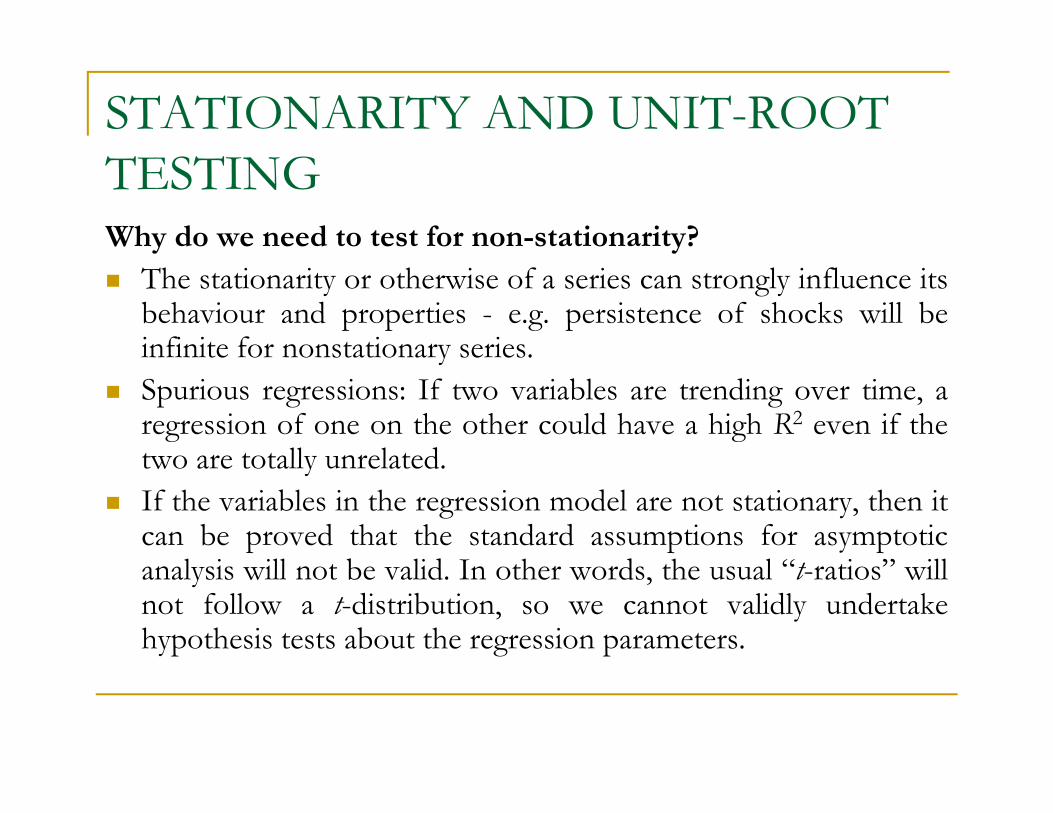
STATIONARITY AND UNIT-ROOT TESTINGWhy do we need to test for non-stationarity?y y

The stationarity or otherwise of a series can strongly influence itsbehaviour and properties - e.g. persistence of shocks will beinfinite for nonstationary series.infinite for nonstationary series.Spurious regressions: If two variables are trending over time, aregression of one on the other could have a high R2 even if thetwo are totally unrelatedtwo are totally unrelated.If the variables in the regression model are not stationary, then itcan be proved that the standard assumptions for asymptotic

l i ill b lid I h d h l “ i ” illanalysis will not be valid. In other words, the usual “t-ratios” willnot follow a t-distribution, so we cannot validly undertakehypothesis tests about the regression parameters.

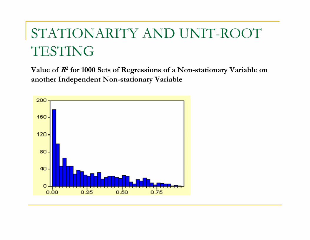
STATIONARITY AND UNIT-ROOT TESTINGValue of R2 for 1000 Sets of Regressions of a Non-stationary Variable on another Independent Non-stationary Variable

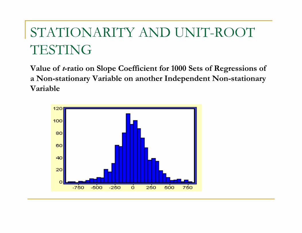
STATIONARITY AND UNIT-ROOT TESTINGValue of t-ratio on Slope Coefficient for 1000 Sets of Regressions of p ga Non-stationary Variable on another Independent Non-stationary Variable

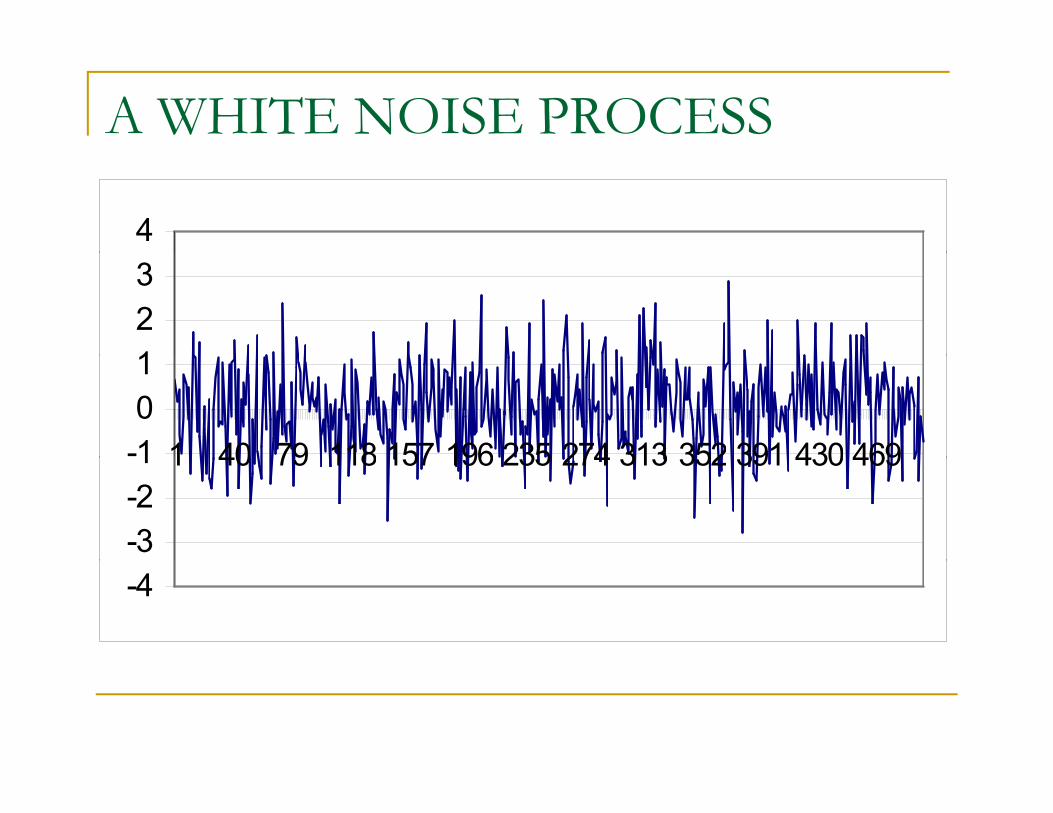
A WHITE NOISE PROCESS

4

123

-101

1 40 79 118 157 196 235 274 313 352 391 430 469

-3-21 1 40 79 118 157 196 235 274 313 352 391 430 469

-4

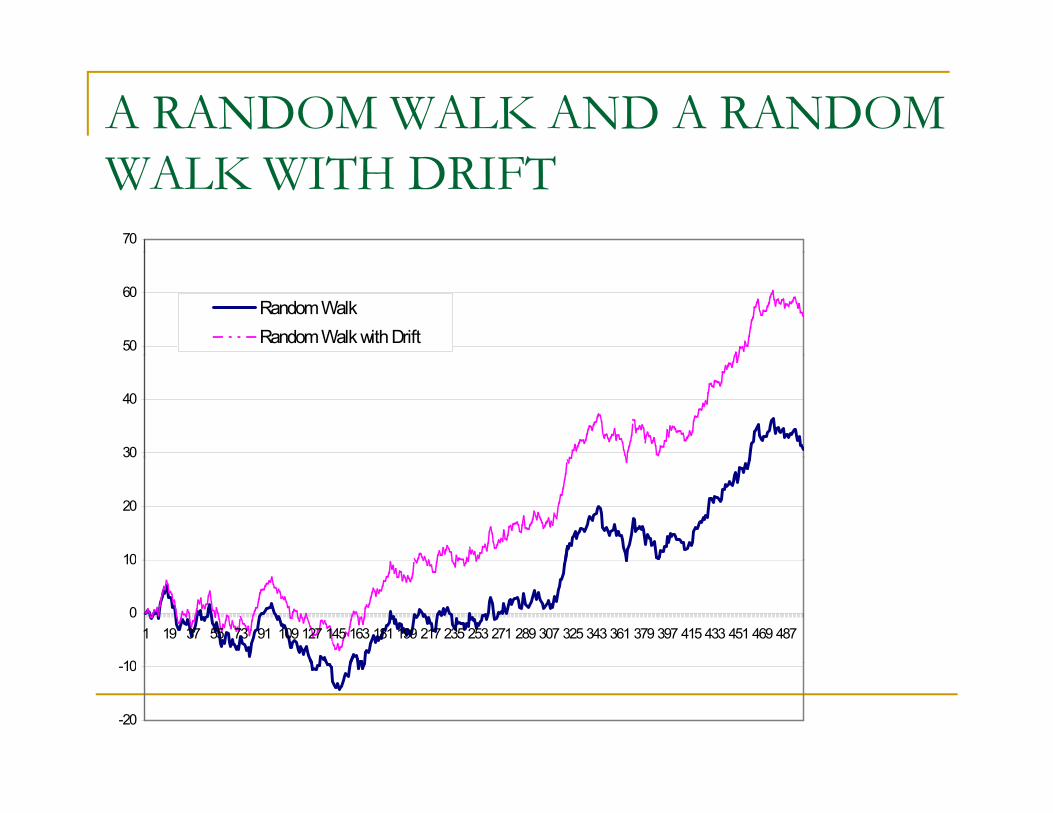
A RANDOM WALK AND A RANDOM WALK WITH DRIFT

70

50

60Random WalkRandom Walk with Drift

30

40

10

20

10

0

10

1 19 37 55 73 91 109 127 145 163 181 199 217 235 253 271 289 307 325 343 361 379 397 415 433 451 469 487

-20

-10

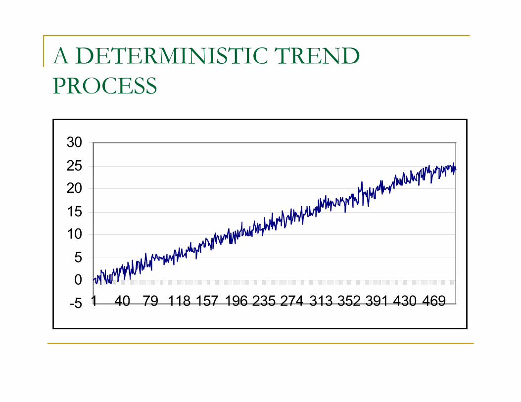
A DETERMINISTIC TREND PROCESS

2530

1520

05

10

-50

1 40 79 118 157 196 235 274 313 352 391 430 469

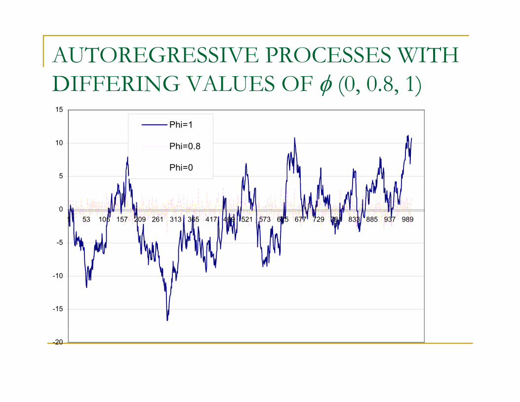
AUTOREGRESSIVE PROCESSES WITH DIFFERING VALUES OF φ (0, 0.8, 1)15

Phi=1

5

10

Phi=1

Phi=0.8

Phi=0

0

5

1 53 105 157 209 261 313 365 417 469 521 573 625 677 729 781 833 885 937 989

-10

-5

-15

10

-20

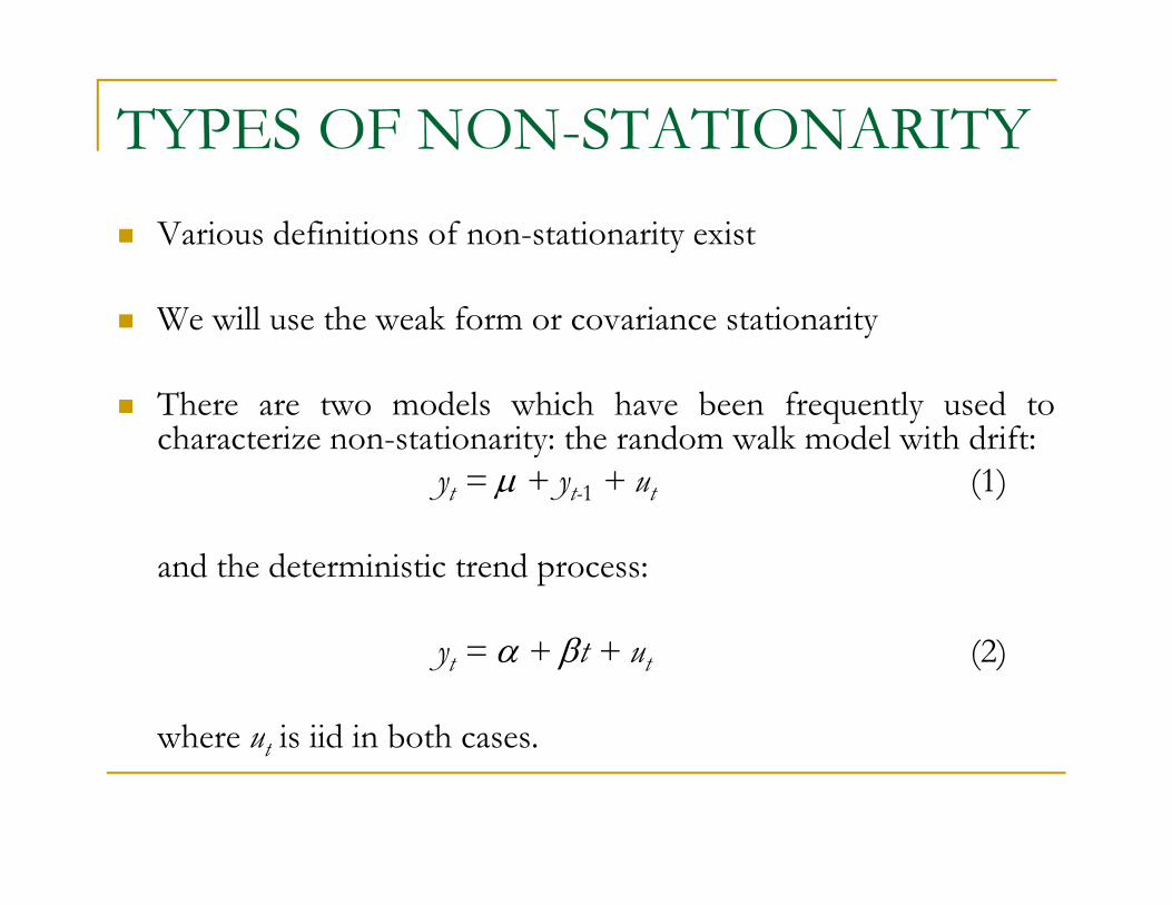
TYPES OF NON-STATIONARITYVarious definitions of non-stationarity exist

We will use the weak form or covariance stationarity

Th d l hi h h b f l dThere are two models which have been frequently used tocharacterize non-stationarity: the random walk model with drift:

yt = μ + yt-1 + ut (1)

and the deterministic trend process:

yt = α + βt + ut (2)

where u is iid in both caseswhere ut is iid in both cases.

STOCHASTIC NON-STATIONARITY

Note that model (1) could be generalized to the case where yt isan explosive process:an explosive process:

yt = μ + φyt-1 + ut

where φ > 1.Typically, the explosive case is ignored and we use φ = 1 tocharacterize the non-stationarity becauseφ d d b d dφ > 1 does not describe many data series in economics andfinance.φ > 1 has an intuitively unappealing property: shocks to theφ > 1 has an intuitively unappealing property: shocks to thesystem are not only persistent through time, they arepropagated so that a given shock will have an increasinglyl i fllarge influence.

STOCHASTIC NON-STATIONARITYTo see this, consider the general case of an AR(1) with no drift:

φyt = φyt-1 + ut (3)Let φ take any value for now.We can write: y 1 = φy 2 + u 1We can write: yt-1 φyt-2 + ut-1

yt-2 = φyt-3 + ut-2Substituting into (3) yields: yt = φ(φyt-2 + ut-1) + ut

= φ2yt-2 + φut-1 + utSubstituting again for yt-2: yt = φ2(φyt-3 + ut-2) + φut-1 + ut

= φ3 y + φ2u + φu + u= φ3 yt-3 + φ ut-2 + φut-1 + utSuccessive substitutions of this type lead to:

yt = φT y0 + φut-1 + φ2ut-2 + φ3ut-3 + ...+ φTu0 + ut

IMPACTS OF SHOCKS TO STATIONARY AND NON-STATIONARY SERIESWe have 3 cases:1. φ<1 ⇒ φT→0 as T→∞

So the shocks to the system gradually die away.2. φ=1 ⇒ φT =1∀ T

So shocks persist in the system and never die away. We obtain:So shocks persist in the system and never die away. We obtain:as T→∞

So just an infinite sum of past shocks plus some starting value ofyy0.

3. φ>1. Now given shocks become more influential as time goes on,since if φ>1, φ3>φ2>φ etc.

DETRENDING A STOCHASTICALLY NON-STATIONARY SERIES

Going back to our 2 characterizations of non-stationarity, the r.w. withd if + + (1)drift: yt = μ + yt-1 + ut (1)and the trend-stationary process

yt = α + βt + ut (2)d dThe two will require different treatments to induce stationarity. The

second case is known as deterministic non-stationarity and what isrequired is detrending.The first case is known as stochastic non stationarity If we letThe first case is known as stochastic non-stationarity. If we let

Δyt = yt - yt-1andIf we take (1) and subtract y 1 from both sides:If we take (1) and subtract yt-1 from both sides:

yt - yt-1 = μ + utΔyt = μ + ut

We say that we have induced stationarity by “differencing once”We say that we have induced stationarity by differencing once .

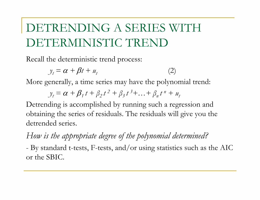
DETRENDING A SERIES WITH DETERMINISTIC TRENDRecall the deterministic trend process: p

yt = α + βt + ut (2)More generally, a time series may have the polynomial trend:

yt = α + β1 t + β2 t 2 + β3 t 3+…+ βn t n + ut

Detrending is accomplished by running such a regression and bt i i th i f id l Th id l ill i thobtaining the series of residuals. The residuals will give you the

detrended series.

How is the appropriate degree of the polynomial determined?How is the appropriate degree of the polynomial determined?- By standard t-tests, F-tests, and/or using statistics such as the AIC or the SBIC.

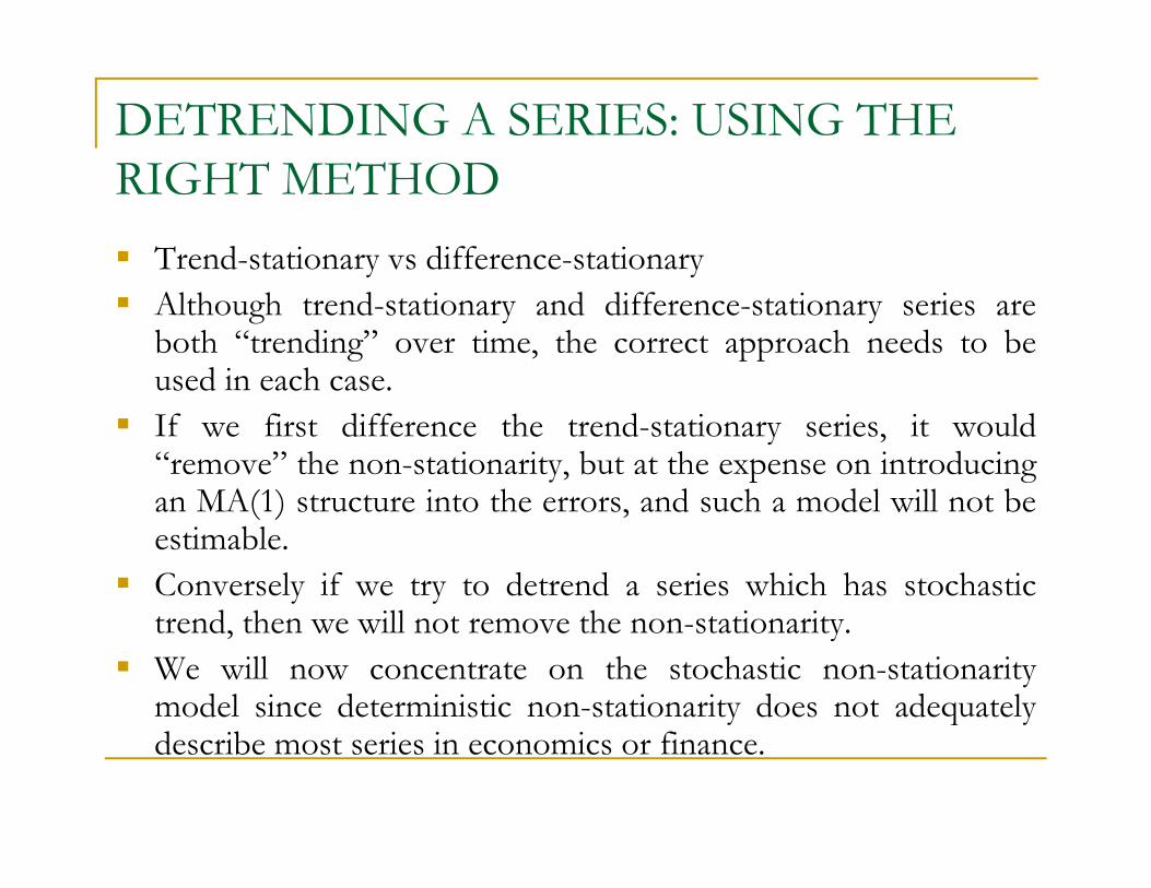
DETRENDING A SERIES: USING THE RIGHT METHODRIGHT METHOD

Trend-stationary vs difference-stationaryy yAlthough trend-stationary and difference-stationary series areboth “trending” over time, the correct approach needs to beused in each case.used in each case.If we first difference the trend-stationary series, it would“remove” the non-stationarity, but at the expense on introducingan MA(1) structure into the errors and such a model will not bean MA(1) structure into the errors, and such a model will not beestimable.Conversely if we try to detrend a series which has stochastic

d h ill h i itrend, then we will not remove the non-stationarity.We will now concentrate on the stochastic non-stationaritymodel since deterministic non-stationarity does not adequatelyy q ydescribe most series in economics or finance.

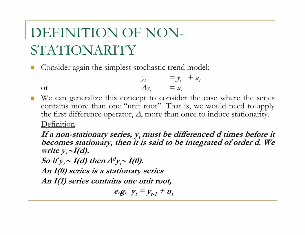
DEFINITION OF NON-STATIONARITY

Consider again the simplest stochastic trend model:yt = yt-1 + ut

or Δyt = utWe can generalize this concept to consider the case where the series

d dcontains more than one “unit root”. That is, we would need to applythe first difference operator, Δ, more than once to induce stationarity.DefinitionIf i i b diff d d i b f iIf a non-stationary series, yt must be differenced d times before itbecomes stationary, then it is said to be integrated of order d. Wewrite yt ∼I(d).So if y ∼ I(d) then Δdy ∼ I(0).So if yt I(d) then Δ yt I(0).An I(0) series is a stationary seriesAn I(1) series contains one unit root,

e g y = y + ue.g. yt = yt-1 + ut

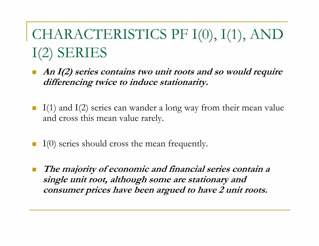
CHARACTERISTICS PF I(0), I(1), AND I(2) SERIES

An I(2) series contains two unit roots and so would require ( ) qdifferencing twice to induce stationarity.

I(1) and I(2) series can wander a long way from their mean valueI(1) and I(2) series can wander a long way from their mean value and cross this mean value rarely.

I(0) series should cross the mean frequently.

The majority of economic and financial series contain aThe majority of economic and financial series contain a single unit root, although some are stationary and consumer prices have been argued to have 2 unit roots.

TESTING FOR UNIT ROOTS: THE DICKEY-FULLER TEST

The early and pioneering work on testing for a unit root in y p g gtime series was done by Dickey and Fuller (Dickey and Fuller 1979, Fuller 1976). The basic objective of the test is to test the null hypothesis that φ =1 in:yp φ

yt = φyt-1 + ut

against the one-sided alternative φ <1. So we have H i i iH0: series contains a unit root

vs. H1: series is stationary. We usually use the regression:W y g

Δyt = ψyt-1 + ut

so that a test of φ=1 is equivalent to a test of ψ=0 (since φ-1 )1=ψ).

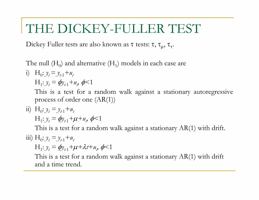
THE DICKEY-FULLER TESTDickey Fuller tests are also known as τ tests: τ, τμ, ττ.

Th ll (H ) d lt r ti (H ) d l i h rThe null (H0) and alternative (H1) models in each case arei) H0: yt = yt-1+ut

H1: yt = φyt-1+ut, φ<1This is a test for a random walk against a stationary autoregressiveprocess of order one (AR(1))

ii) H0: yt = yt-1+ut) 0 yt yt 1 tH1: yt = φyt-1+μ+ut, φ<1This is a test for a random walk against a stationary AR(1) with drift.

iii) H : y = y +uiii) H0: yt = yt-1+utH1: yt = φyt-1+μ+λt+ut, φ<1This is a test for a random walk against a stationary AR(1) with drift

d ti t dand a time trend.

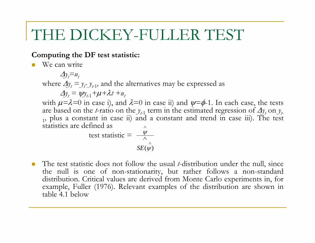
THE DICKEY-FULLER TESTComputing the DF test statistic:

We can writeΔyt=utΔyt ut

where Δyt = yt- yt-1, and the alternatives may be expressed asΔyt = ψyt-1+μ+λt +ut

with μ=λ=0 in case i), and λ=0 in case ii) and ψ=φ-1. In each case, the testsμ ), ) ψ φ ,are based on the t-ratio on the yt-1 term in the estimated regression of Δyt on yt-1, plus a constant in case ii) and a constant and trend in case iii). The teststatistics are defined as

test statistic = ψ∧

test statistic

The test statistic does not follow the usual t-distribution under the null, since

ψ∧

∧

SE( )

the null is one of non-stationarity, but rather follows a non-standarddistribution. Critical values are derived from Monte Carlo experiments in, forexample, Fuller (1976). Relevant examples of the distribution are shown intable 4.1 below

THE DICKEY-FULLER TEST

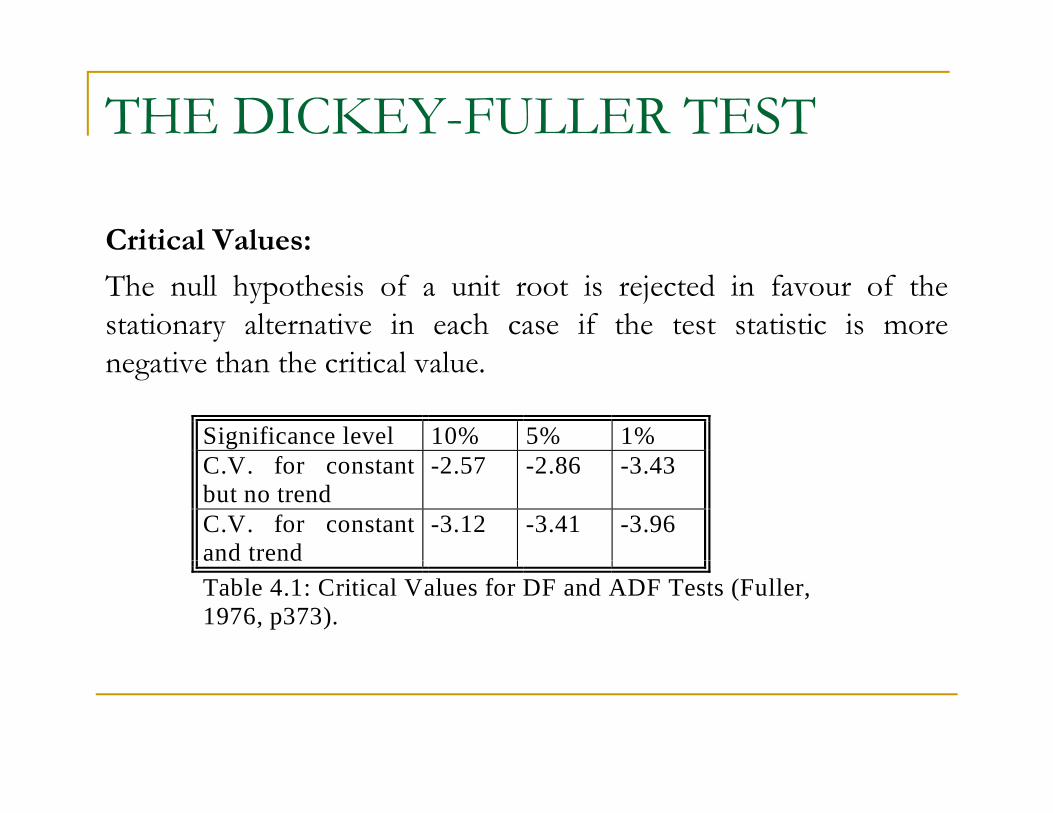
Critical Values:

The null hypothesis of a unit root is rejected in favour of thestationary alternative in each case if the test statistic is more

i h h i i l lnegative than the critical value.

Significance level 10% 5% 1%C V f 2 57 2 86 3 43C.V. for constantbut no trend

-2.57 -2.86 -3.43

C.V. for constantand trend

-3.12 -3.41 -3.96and trendTable 4.1: Critical Values for DF and ADF Tests (Fuller,1976, p373).

TESTING FOR UNIT ROOTS: THE AUGMENTED DICKEY-FULLER TEST

The tests above are only valid if ut is white noise. In particular, ut willbe autocorrelated if there was autocorrelation in the dependentvariable of the regression (Δyt) which we have not modelled. Thesolution is to “augment” the test using p lags of the dependent

i bl Th l i d l i (i) i ivariable. The alternative model in case (i) is now written:

∑=

−− +Δ+=Δp

itititt uyyy

11 αψ

The same critical values from the DF tables are used as before. Aproblem now arises in determining the optimal number of lags of thedependent variable.There are 2 ways- use the frequency of the data to decide- use information criteriause information criteria

TESTING FOR HIGHER ORDERS OF INTEGRATIONINTEGRATION

Consider the simple regression:Δyt = ψyt 1 + utyt ψyt-1 t

We test H0: ψ=0 vs. H1: ψ<0.If H0 is rejected we simply conclude that yt does not contain aunit rootunit root.But what do we conclude if H0 is not rejected? The seriescontains a unit root, but is that it? No! What if yt∼I(2)? We wouldstill not have rejected. So we now need to teststill not have rejected. So we now need to test

H0: yt∼I(2) vs. H1: yt∼I(1)We would continue to test for a further unit root until we rejectedHH0.We now regress Δ2yt on Δyt-1 (plus lags of Δ2yt if necessary).Now we test H0: Δyt∼I(1) which is equivalent to H0: yt∼I(2).So in this case, if we do not reject (unlikely), we conclude that ytis at least I(2).

TESTING FOR UNIT ROOTS: THE PHILLIPS-PERRON TEST

Phillips and Perron have developed a more comprehensive p p ptheory of unit root nonstationarity. The tests are similar to ADF tests, but they incorporate an automatic correction to the DF procedure to allow for autocorrelated residualsprocedure to allow for autocorrelated residuals.

The tests usually give the same conclusions as the ADF tests, y g ,and the calculation of the test statistics is complex.

CRITICISMS OF DICKEY-FULLER AND PHILLIPS PERRON TYPE TESTS

Main criticism is that the power of the tests is low if the process is stationary but with a root close to the non-stationary boundary.e.g. the tests are poor at deciding if

φ=1 or φ=0.95,φ φ ,especially with small sample sizes.

If the true data generating process (dgp) isIf the true data generating process (dgp) is yt = 0.95yt-1 + ut

then the null hypothesis of a unit root should be rejected.

One way to get around this is to use a stationarity test as well as the unit root tests we have looked at.

STATIONARITY TESTS

Stationarity tests haveH0: yt is stationary

versus H1: yt is non-stationary

So that by default under the null the data will appear stationary.

O h i i i h KPSS (K i ki PhilliOne such stationarity test is the KPSS test (Kwaitowski, Phillips, Schmidt and Shin, 1992).

Thus we can compare the results of these tests with the ADF/PP procedure to see if we obtain the same conclusion.

Exercise

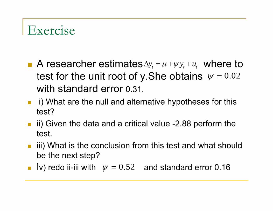
A researcher estimates where toy y uμ ψΔ = + +A researcher estimates where to test for the unit root of y.She obtainswith standard error 0.31.

t t ty y uμ ψΔ + +0.02ψ =

i) What are the null and alternative hypotheses for this test? ii) Given the data and a critical value -2.88 perform the test. iii) What is the conclusion from this test and what shouldiii) What is the conclusion from this test and what should be the next step?İv) redo ii-iii with and standard error 0.160.52ψ =

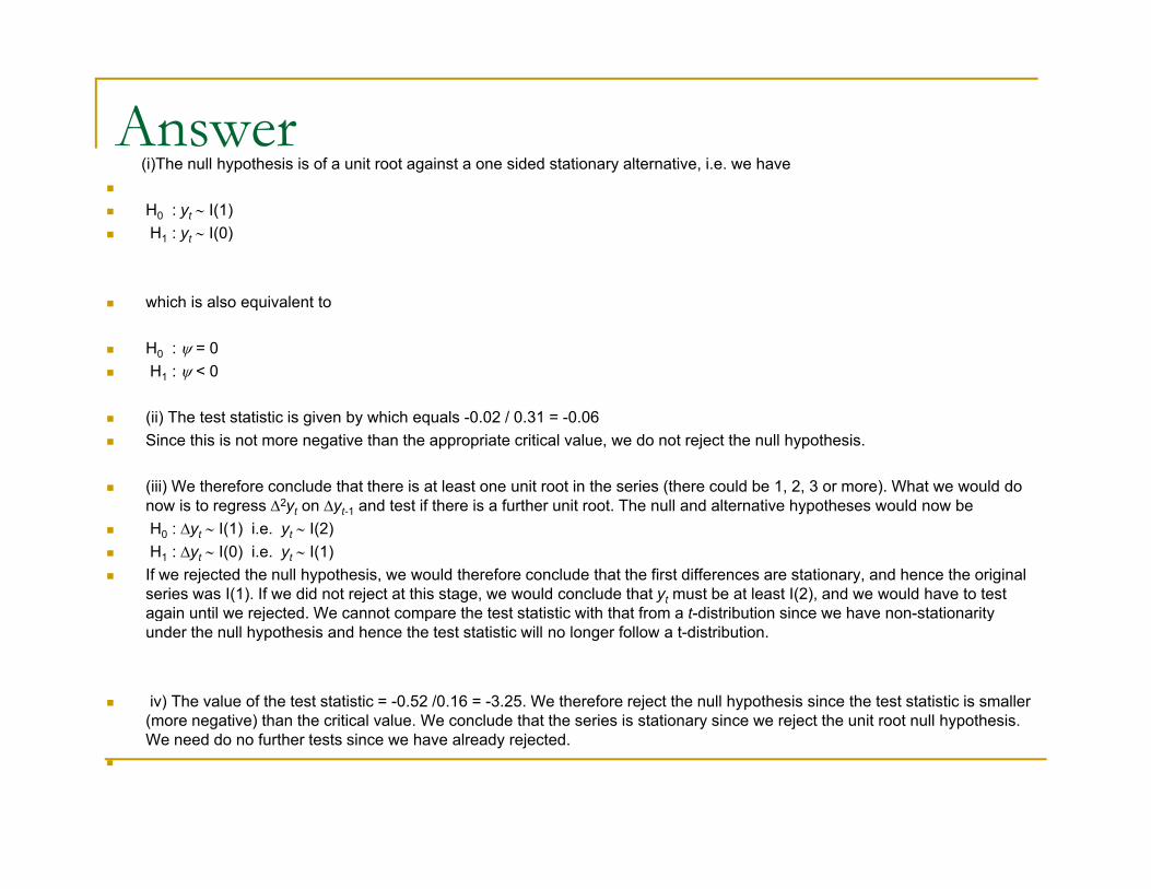
Answer(i)The null hypothesis is of a unit root against a one sided stationary alternative i e we have(i)The null hypothesis is of a unit root against a one sided stationary alternative, i.e. we have

H0 : yt ∼ I(1)H1 : yt ∼ I(0)

which is also equivalent to

H0 : ψ = 0H1 : ψ < 0

(ii) The test statistic is given by which equals -0.02 / 0.31 = -0.06Since this is not more negative than the appropriate critical value, we do not reject the null hypothesis.

(iii) We therefore conclude that there is at least one unit root in the series (there could be 1, 2, 3 or more). What we would doi t Δ2 Δ d t t if th i f th it t Th ll d lt ti h th ld bnow is to regress Δ2yt on Δyt-1 and test if there is a further unit root. The null and alternative hypotheses would now be

H0 : Δyt ∼ I(1) i.e. yt ∼ I(2)H1 : Δyt ∼ I(0) i.e. yt ∼ I(1)If we rejected the null hypothesis, we would therefore conclude that the first differences are stationary, and hence the original series was I(1). If we did not reject at this stage, we would conclude that yt must be at least I(2), and we would have to test again until we rejected We cannot compare the test statistic with that from a t distribution since we have non stationarityagain until we rejected. We cannot compare the test statistic with that from a t-distribution since we have non-stationarity under the null hypothesis and hence the test statistic will no longer follow a t-distribution.

iv) The value of the test statistic = -0.52 /0.16 = -3.25. We therefore reject the null hypothesis since the test statistic is smaller (more negative) than the critical value. We conclude that the series is stationary since we reject the unit root null hypothesis.(more negative) than the critical value. We conclude that the series is stationary since we reject the unit root null hypothesis. We need do no further tests since we have already rejected.

Question

1.) What kinds of variables are likely to be non-1.) What kinds of variables are likely to be nonstationary?

2 ) Why is it important to test for non-stationarity2.) Why is it important to test for non stationarity before estimation?

Answer

1. Many series in finance and economics in their levels (or log-levels) forms are non-stationary and exhibit stochastic trends They have a tendency not to revert to a mean level but they “wander” for prolonged periods instochastic trends. They have a tendency not to revert to a mean level, but they wander for prolonged periods in one direction or the other. Examples would be most kinds of asset or goods prices, GDP, unemployment, money supply, etc. Such variables can usually be made stationary by transforming them into their differences or by constructing percentage changes of them.

2. Non-stationarity can be an important determinant of the properties of a series. Also, if two series are non-i i h bl f “ i ” i Thi hstationary, we may experience the problem of “spurious” regression. This occurs when we regress one non-

stationary variable on a completely unrelated non-stationary variable, but yield a reasonably high value of R2, apparently indicating that the model fits well. Most importantly therefore, we are not able to perform any hypothesis tests in models which inappropriately use non-stationary data since the test statistics will no longer follow the distributions which we assumed they would (e.g. a t or F), so any inferences we make are likely to be invalidinvalid.

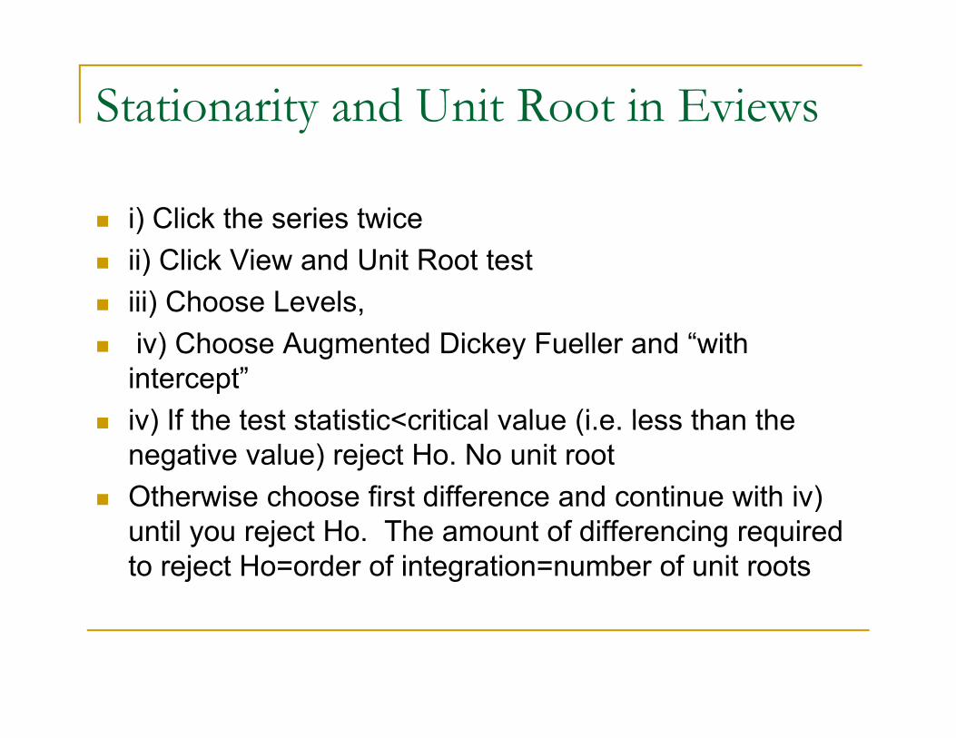
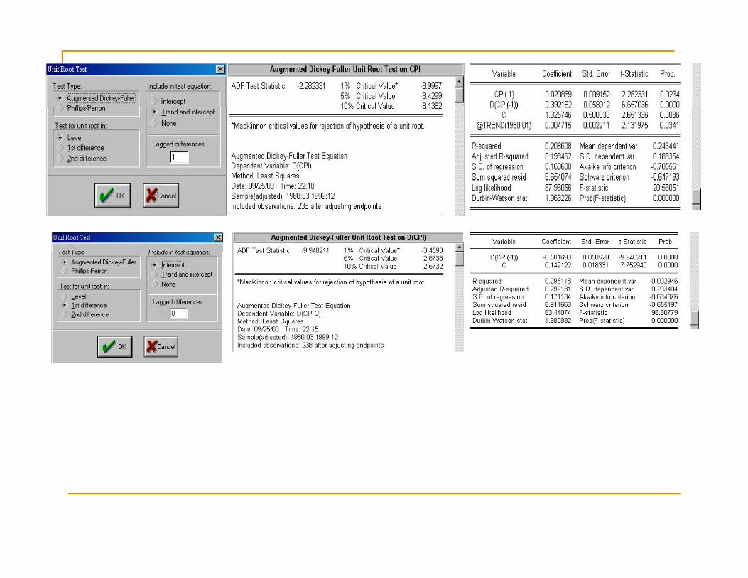
Stationarity and Unit Root in Eviews

i) Click the series twice)ii) Click View and Unit Root testiii) Choose Levels,iv) Choose Augmented Dickey Fueller and “with intercept”iv) If the test statistic<critical value (i e less than theiv) If the test statistic<critical value (i.e. less than the negative value) reject Ho. No unit rootOtherwise choose first difference and continue with iv) )until you reject Ho. The amount of differencing required to reject Ho=order of integration=number of unit roots

��������

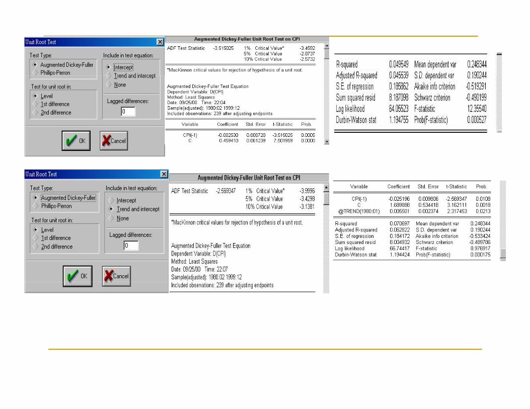
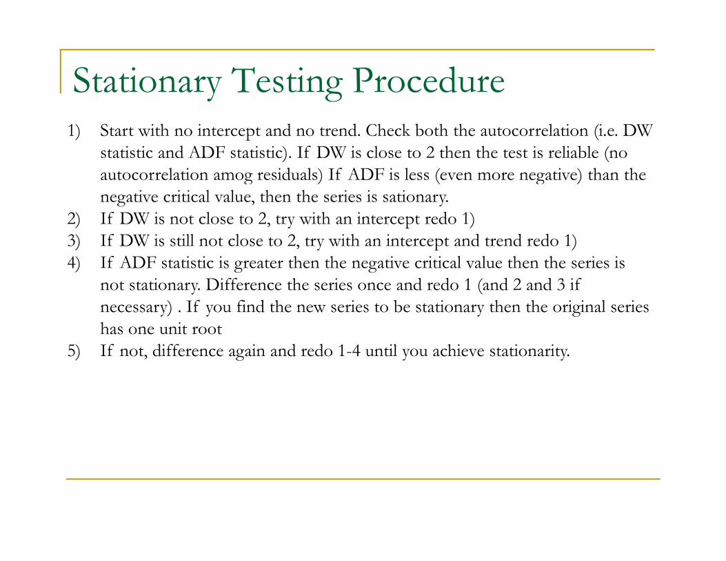
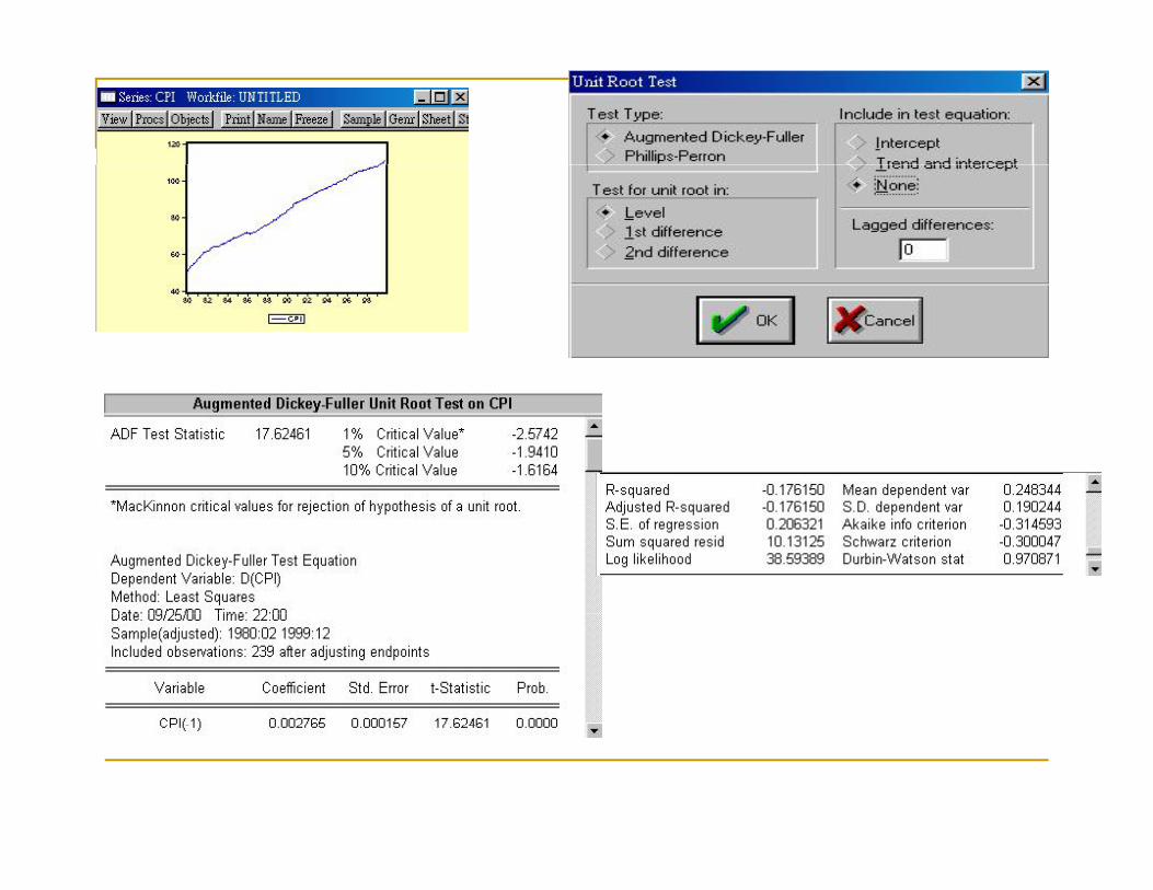
Stationary Testing Procedure1) Start with no intercept and no trend. Check both the autocorrelation (i.e. DW

statistic and ADF statistic). If DW is close to 2 then the test is reliable (no autocorrelation amog residuals) If ADF is less (even more negative) than theautocorrelation amog residuals) If ADF is less (even more negative) than the negative critical value, then the series is sationary.

2) If DW is not close to 2, try with an intercept redo 1)3) If DW is still not close to 2, try with an intercept and trend redo 1)3) If DW is still not close to 2, try with an intercept and trend redo 1)4) If ADF statistic is greater then the negative critical value then the series is

not stationary. Difference the series once and redo 1 (and 2 and 3 if necessary) . If you find the new series to be stationary then the original series y) y y ghas one unit root

5) If not, difference again and redo 1-4 until you achieve stationarity.

COINTEGRATION

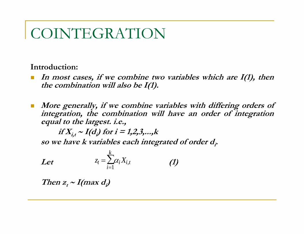
Introduction:In most cases, if we combine two variables which are I(1), thenthe combination will also be I(1).

More generally, if we combine variables with differing orders ofintegration, the combination will have an order of integrationequal to the largest. i.e.,

if X ∼ I(d ) for i = 1 2 3 kif Xi,t ∼ I(di) for i = 1,2,3,...,kso we have k variables each integrated of order di.

Let (1)z Xt i i t

k=∑αLet (1)

Then zt ∼ I(max di)

z Xt i i ti

==∑α ,

1

COINTEGRATION

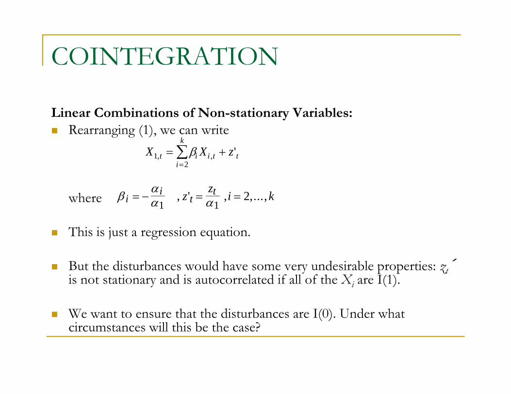
Linear Combinations of Non-stationary Variables:Rearranging (1), we can write

X X zt i i t ti

k

12

, , '= +=∑β

where βαα αi

it

tz z i k= − = =1 1

2, ' , ,...,

This is just a regression equation.

But the disturbances would have some very undesirable properties: zt´y p p ztis not stationary and is autocorrelated if all of the Xi are I(1).

We want to ensure that the disturbances are I(0). Under what circumstances will this be the case?

COINTEGRATIONDefinition of Cointegration (Engle & Granger, 1987)

Let zt be a k×1 vector of variables, then the components of zt aret p ztcointegrated of order (d,b) ifi) All components of zt are I(d)ii) There is at least one vector of coefficients α such that α ′z ∼ii) There is at least one vector of coefficients α such that α ztI(d-b)Many time series are non-stationary but “move together” over time.If i bl i d i h li bi i fIf variables are cointegrated, it means that a linear combination ofthem will be stationary.There may be up to r linearly independent cointegrating

l i hi ( h k 1) l k i irelationships (where r ≤ k-1), also known as cointegrating vectors. ris also known as the cointegrating rank of zt.A cointegrating relationship may also be seen as a long termrelationship.

COINTEGRATION

Cointegration and Equilibrium:Examples of possible Cointegrating Relationships in finance and economics:

spot and futures pricesdratio of relative prices and an exchange rate

equity prices and dividendsreal money balances, real GDP and the determinants of velocity

Market forces arising from no arbitrage conditions should ensure an equilibrium relationship. (UIP, etc.)

No cointegration implies that series could wander apart without bound in the long run.

EQUILIBRIUM CORRECTION OR ERROR CORRECTION MODELS

When the concept of non-stationarity was first considered, a usuali d d l k h fi diff f i fresponse was to independently take the first differences of a series of

I(1) variables.

Th pr bl m ith thi ppr h i th t p r fir t diff r m d lThe problem with this approach is that pure first difference modelshave no long run solution.e.g. Consider yt and xt both I(1).The model we may want to estimate isThe model we may want to estimate is

Δ yt = βΔxt + utBut this collapses to nothing in the long run.

The definition of the long run that we use is whereyt = yt-1 = y; xt = xt-1 = x.

Hence all the difference terms will be zero i e Δ y = 0; Δx = 0Hence all the difference terms will be zero, i.e. Δ yt = 0; Δxt = 0.

EQUILIBRIUM CORRECTION OR ERROR CORRECTION MODELSSpecifying an ECM:

One way to get around this problem is to use both first difference and levels terms, e.g.

Δ yt = β1Δxt + β2(yt 1-γxt 1) + ut (2)yt β1 t β2(yt-1 γ t-1) t ( )yt-1-γxt-1 is known as the error correction term.

Providing that y and x are cointegrated with cointegrating coefficientProviding that yt and xt are cointegrated with cointegrating coefficient γ, then (yt-1-γxt-1) will be I(0) even though the constituents are I(1).

W h lidl OLS (2)We can thus validly use OLS on (2).

The Granger representation theorem shows that any cointegrating relationship can be expressed as an equilibrium correction model.

TESTING FOR COINTEGRATION

The model for the equilibrium correction term can be generalized toinclude more than two variables:

yt = β1 + β2x2t + β3x3t + … + βkxkt + ut (3)

ut should be I(0) if the variables yt, x2t, ... xkt are cointegrated.

So what if we want to test is the residuals of equation (3) to see if theySo what if we want to test is the residuals of equation (3) to see if theyare non-stationary or stationary. We can use the DF / ADF test on ut.So we have the regression

i h iidΔ with vt ∼ iid.

However, since this is a test on the residuals of an actual model, ,

Δu u vt t t= +−ψ 1

utthen the critical values are changed.

TESTING FOR COINTEGRATION

Engle and Granger (1987) have tabulated a new set of criticalg g ( )values and hence the test is known as the Engle Granger (E.G.)test.

We can also use the Durbin Watson test statistic or the PhillipsPerron approach to test for non-stationarity of .ut

What are the null and alternative hypotheses for a test on theresiduals of a potentially cointegrating regression?p g g gH0 : unit root in cointegrating regression’s residualsH1 : residuals from cointegrating regression are stationary

ESTIMATION IN COINTEGRATED SYSTEMS: THE ENGEL GRANGER APPROACHTHE ENGEL-GRANGER APPROACH

There are (at least) 3 methods we could use: Engle Granger, Engle andY d J hYoo, and Johansen.The Engle Granger 2 Step MethodThis is a single equation technique which is conducted as follows:Step 1:- Make sure that all the individual variables are I(1).- Then estimate the cointegrating regression using OLS.- Save the residuals of the cointegrating regression, .- Test these residuals to ensure that they are I(0).Step 2:- Use the step 1 residuals as one variable in the error correction model e.g.

Δ yt = β1Δxt + β2( z ) + utˆ

1ˆ −tuˆwhere z= yt-1- xt-11ˆ −tu γ

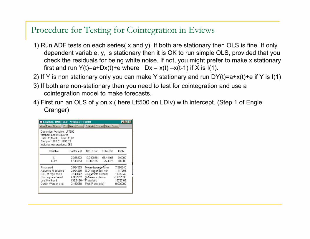
Procedure for Testing for Cointegration in Eviews1) Run ADF tests on each series( x and y) If both are stationary then OLS is fine If only1) Run ADF tests on each series( x and y). If both are stationary then OLS is fine. If only

dependent variable, y, is stationary then it is OK to run simple OLS, provided that you check the residuals for being white noise. If not, you might prefer to make x stationary first and run Y(t)=a+Dx(t)+e where Dx = x(t) –x(t-1) if X is I(1).

) f ( ) ( ) f ( )2) If Y is non stationary only you can make Y stationary and run DY(t)=a+x(t)+e if Y is I(1)3) If both are non-stationary then you need to test for cointegration and use a

cointegration model to make forecasts.4) First run an OLS of y on x ( here Lft500 on LDIv) with intercept. (Step 1 of Engle ) y ( ) p ( p g

Granger)

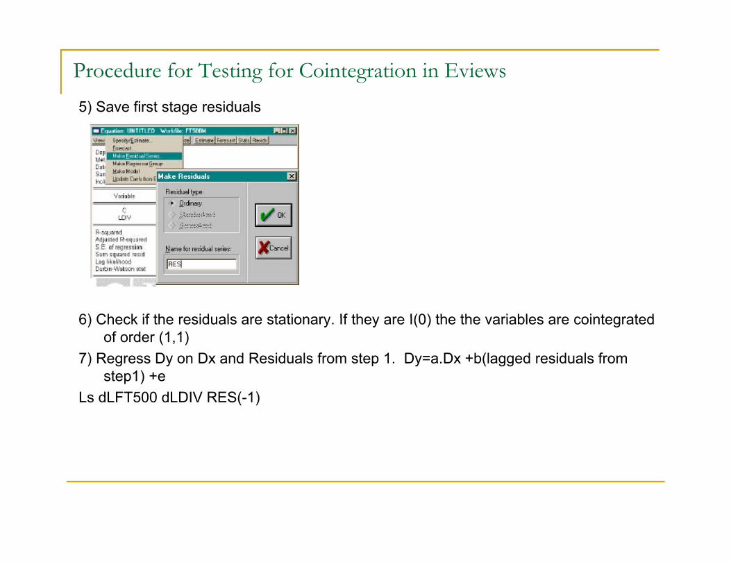
Procedure for Testing for Cointegration in Eviews5) Save first stage residuals5) Save first stage residuals

6) Check if the residuals are stationary If they are I(0) the the variables are cointegrated6) Check if the residuals are stationary. If they are I(0) the the variables are cointegrated of order (1,1)

7) Regress Dy on Dx and Residuals from step 1. Dy=a.Dx +b(lagged residuals from step1) +e

Ls dLFT500 dLDIV RES(-1)

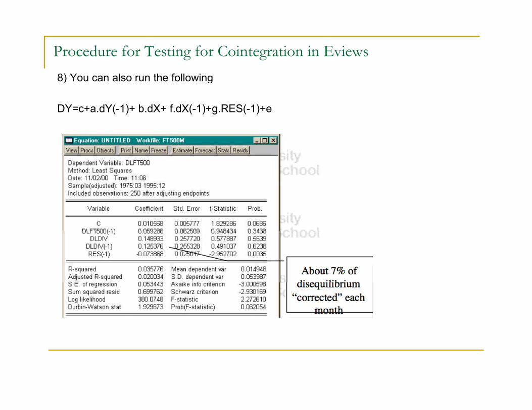
Procedure for Testing for Cointegration in Eviews8) You can also run the following8) You can also run the following

DY=c+a.dY(-1)+ b.dX+ f.dX(-1)+g.RES(-1)+e

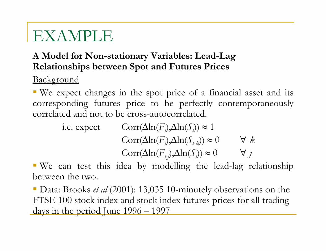
EXAMPLEA Model for Non-stationary Variables: Lead-Lag Relationships between Spot and Futures PricesB k dBackground

We expect changes in the spot price of a financial asset and itscorresponding futures price to be perfectly contemporaneouslycorrelated and not to be cross-autocorrelated.

i.e. expect Corr(Δln(Ft),Δln(St)) ≈ 1Corr(Δln(F ) Δln(S k)) ≈ 0 ∀ kCorr(Δln(Ft),Δln(St-k)) ≈ 0 ∀ kCorr(Δln(Ft-j),Δln(St)) ≈ 0 ∀ j

We can test this idea by modelling the lead-lag relationshipb hbetween the two.

Data: Brooks et al (2001): 13,035 10-minutely observations on the FTSE 100 stock index and stock index futures prices for all trading p gdays in the period June 1996 – 1997

EXAMPLE (CONTINUED)

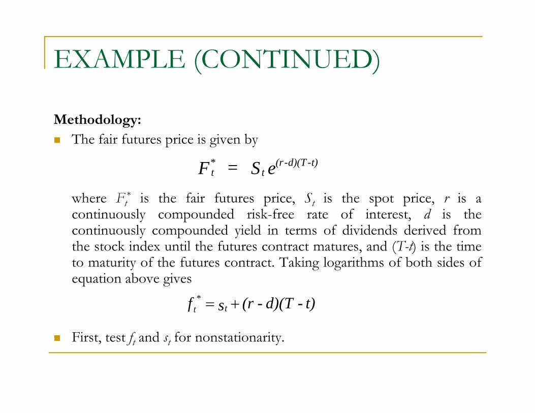
Methodology:The fair futures price is given by

t*

t(r-d)(T-t)F = S e

where Ft* is the fair futures price, St is the spot price, r is a

continuously compounded risk-free rate of interest, d is thecontinuously compounded yield in terms of dividends derived fromcontinuously compounded yield in terms of dividends derived fromthe stock index until the futures contract matures, and (T-t) is the timeto maturity of the futures contract. Taking logarithms of both sides ofequation above givesq g

First test f and s for nonstationarity

t)-d)(T-(r s f tt +=*

First, test ft and st for nonstationarity.

EXAMPLE (CONTINUED)

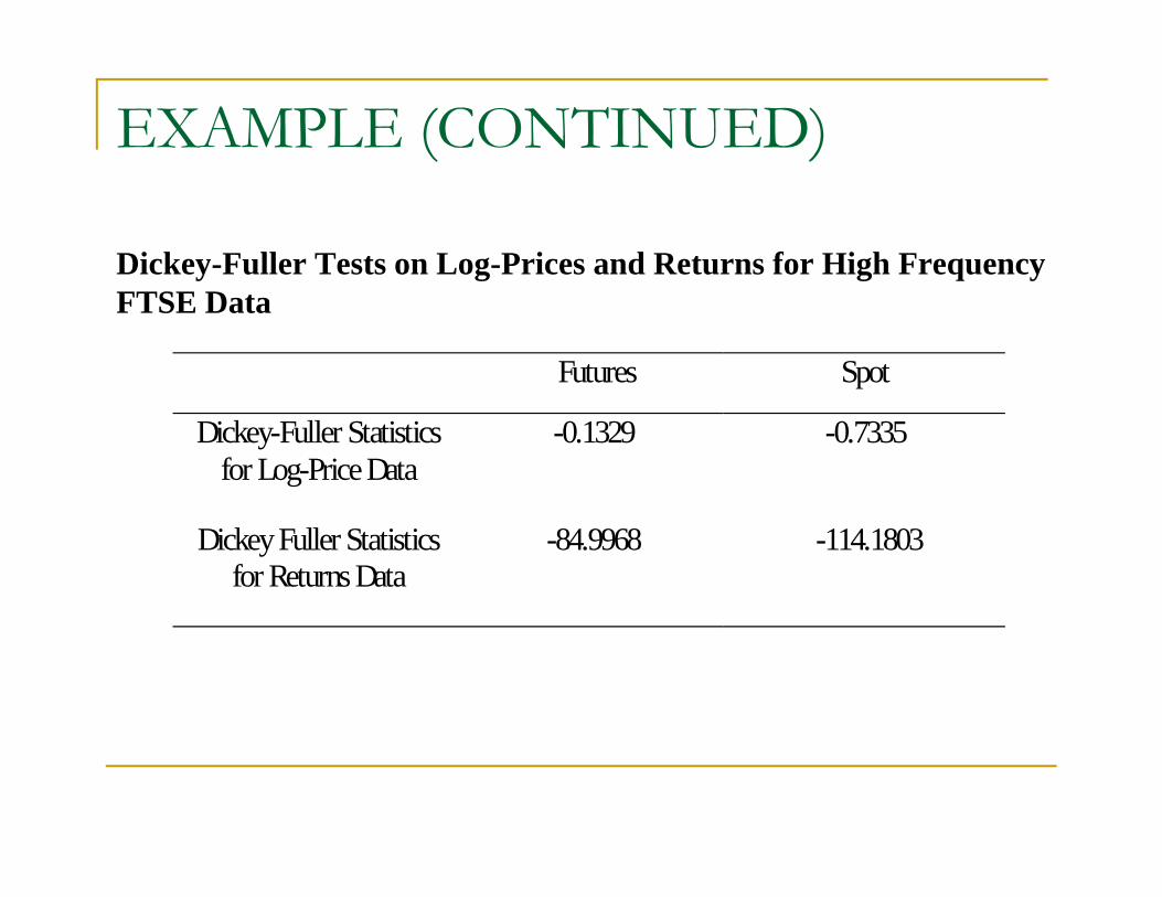
Dickey-Fuller Tests on Log-Prices and Returns for High Frequency y g g q yFTSE Data

Futures Spot

Dickey-Fuller Statisticsfor Log-Price Data

-0.1329 -0.7335

Dickey Fuller Statisticsfor Returns Data

-84.9968 -114.1803

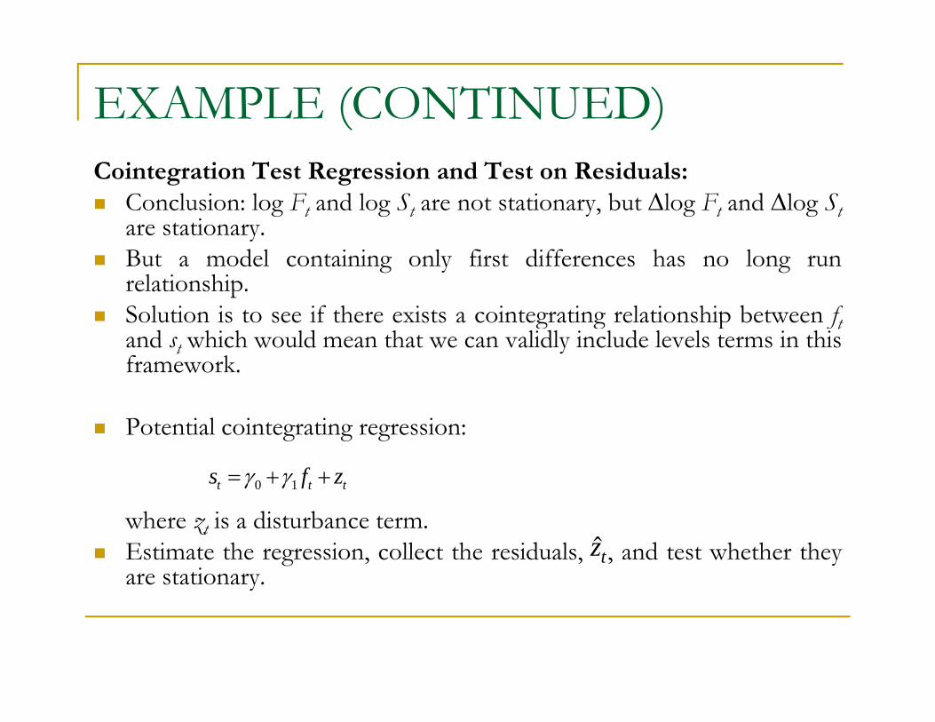
EXAMPLE (CONTINUED)Cointegration Test Regression and Test on Residuals:

Conclusion: log Ft and log St are not stationary, but Δlog Ft and Δlog Stare stationarare stationary.But a model containing only first differences has no long runrelationship.Solution is to see if there exists a cointegrating relationship between fSolution is to see if there exists a cointegrating relationship between ftand st which would mean that we can validly include levels terms in thisframework.

Potential cointegrating regression:

ttt zfs ++= 10 γγ

where zt is a disturbance term.Estimate the regression, collect the residuals, , and test whether theyare stationary.

zty

EXAMPLE (CONTINUED)

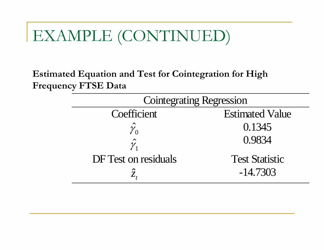
Estimated Equation and Test for Cointegration for High q g gFrequency FTSE Data

Cointegrating RegressionCoefficient

γ 0

Estimated Value0.13450 9834γ10.9834

DF Test on residualsz

Test Statistic14 7303tz -14.7303

EXAMPLE (CONTINUED)

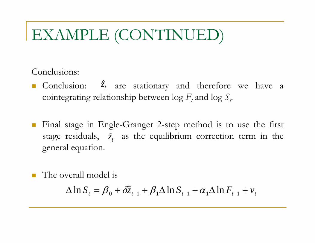
Conclusions:Conclusion: are stationary and therefore we have acointegrating relationship between log Ft and log St.

zt

Final stage in Engle-Granger 2-step method is to use the firststage residuals as the equilibrium correction term in thezstage residuals, as the equilibrium correction term in thegeneral equation.

zt

The overall model is

ttttt vFSzS +Δ+Δ++=Δ −−− 111110 lnlnˆln αβδβ

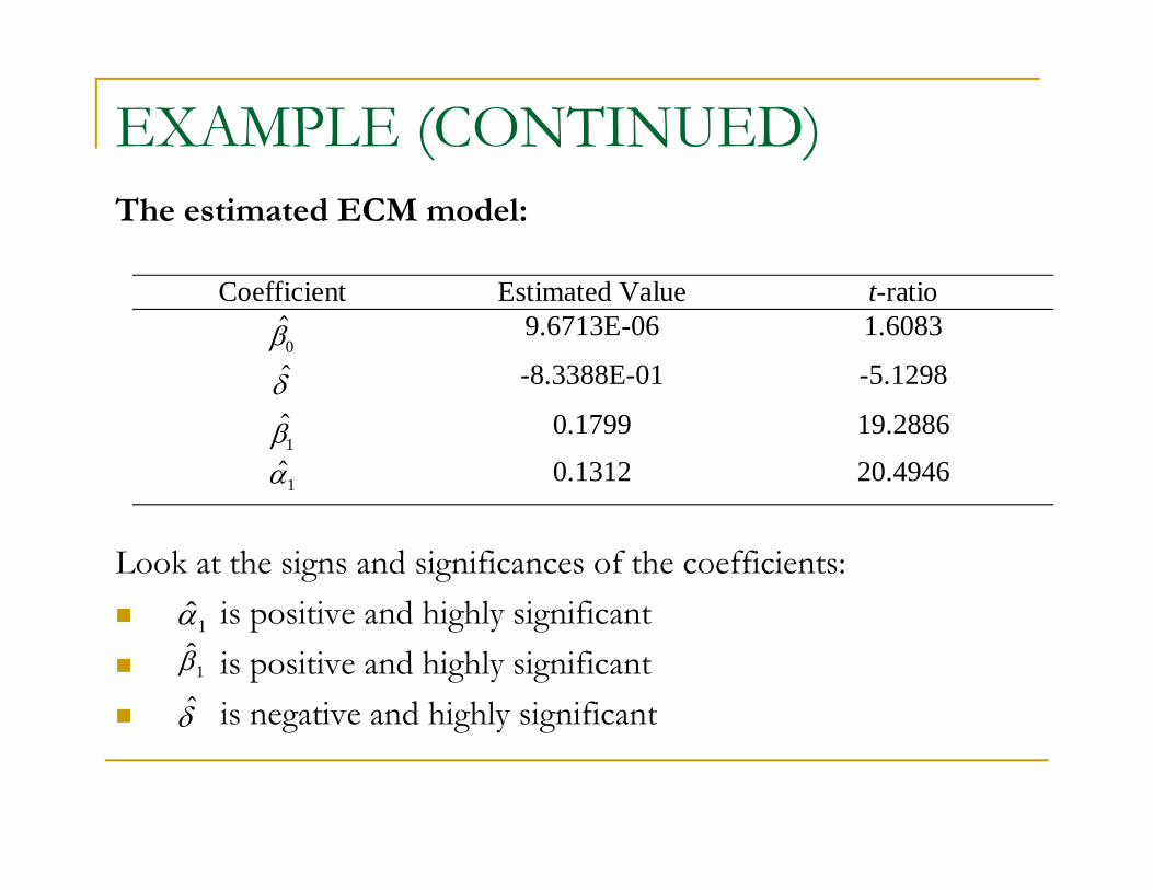
EXAMPLE (CONTINUED)The estimated ECM model:

Coefficient Estimated Value t-ratioβ0

9.6713E-06 1.6083

δ -8.3388E-01 -5.1298δ

β10.1799 19.2886

α1 0.1312 20.4946

Look at the signs and significances of the coefficients:is positive and highly significantα is positive and highly significantis positive and highly significantis negative and highly significant

1α

1β

δ g g y gδ

THE ENGLE-GRANGER APPROACH: SOME DRAWBACKSThis method suffers from a number of problems:

1. Unit root and cointegration tests have low power in finite samples2. We are forced to treat the variables asymmetrically and to specify one as the dependent and the other as independent variables.p p3. Cannot perform any hypothesis tests about the actual cointegrating relationship estimated at stage 1.

- Problem 1 is a small sample problem that should disappear asymptotically.

Problem 2 is addressed by the Johansen approach- Problem 2 is addressed by the Johansen approach.- Problem 3 is addressed by the Engle and Yoo approach or the Johansen approach.

THE ENGLE-YOO 3-STEP METHODOne of the problems with the EG 2-step method is that we cannotmake any inferences about the actual cointegrating regression.

The Engle & Yoo (EY) 3-step procedure takes its first two steps fromEG.

EY add a third step giving updated estimates of the cointegratingvector and its standard errors.

The most important problem with both these techniques is that in thegeneral case above, where we have more than two variables which maybe cointegrated, there could be more than one cointegratingr l ti n hiprelationship.

In fact there can be up to r linearly independent cointegrating vectors( h ≤ 1) h i h b f i bl i l(where r ≤ g-1), where g is the number of variables in total.

THE ENGLE-YOO 3-STEP METHOD

So, in the case where we just had y and x, then r can only be oneor zero.

But in the general case there could be more cointegratingg g grelationships.

And if there are others, how do we know how many there are ord t e e a e ot e s, ow do we ow ow a y t e e a e owhether we have found the “best”?

The answer to this is to use a systems approach to cointegrationThe answer to this is to use a systems approach to cointegration which will allow determination of all r cointegrating relationships - Johansen’s method.