Embed Size (px)
Citation preview
Tensor completion and low-n-rank tensor recovery
via convex optimization
Silvia Gandy1, Benjamin Recht2 and Isao Yamada1
24 January 20111 Tokyo Institute of TechnologyDepartment of Communications and Integrated SystemsMeguro-ku, Ookayama 2-12-1-S3-60152-8550 Tokyo, Japan
2 University of WisconsinComputer Sciences Department1210 W Dayton St Madison, WI 53706
E-mail: [email protected], [email protected],[email protected]
Abstract. In this paper we consider sparsity on a tensor level, as given bythe n-rank of a tensor. In the important sparse-vector approximation problem(compressed sensing) and the low-rank matrix recovery problem, using a convexrelaxation technique proved to be a valuable solution strategy. Here, we will adaptthese techniques to the tensor setting. We use the n-rank of a tensor as sparsitymeasure and consider the low-n-rank tensor recovery problem, i.e., the problem offinding the tensor of lowest n-rank that fulfills some linear constraints. We intro-duce a tractable convex relaxation of the n-rank and propose efficient algorithmsto solve the low-n-rank tensor recovery problem numerically. The algorithms arebased on the Douglas-Rachford splitting technique and its dual variant, the alter-nating direction method of multipliers (ADM).
Keywords: tensor completion, n-rank, nuclear norm, sparsity, Douglas-Rachfordsplitting, alternating direction method of multipliers (ADM)
Tensor completion and low-n-rank tensor recovery via convex optimization 2
1. Introduction
Tensors are the higher-order generalization of vectors and matrices. They have manyapplications in the physical, imaging and information sciences, and an in depthsurvey can be found in [1]. Tensor decompositions give a concise representationof the underlying structure of the tensor, revealing when the tensor-data can bemodeled as lying close to a low-dimensional subspace. Tensor decompositions serve asuseful tools for data summarization in numerous applications, including chemometrics,psychometrics and higher order statistics.
In this work we do not focus on finding the decomposition of a given tensor. Wewill try to recover a tensor by assuming that it is ‘sparse’ in some sense and minimizea sparsity-measure over all tensors that fit the given data. As sparsity-measure weconsider the n-rank of the tensor, i.e., the ranks of the unfoldings of the tensor. Theunfoldings of the tensor are conversions of the tensor into a matrix. The informationwe have about the tensor is modeled as the image of the underlying tensor under aknown linear mapping. One example of such a map is the sampling of a subset ofthe entries of the tensor. This problem is called the tensor completion problem; it isa missing value estimation problem. In computer graphics missing value estimationsproblem are known as in-painting problems and appear for images, videos, etc.
The approaches for completing the tensor can coarsely be divided into local andglobal approaches. A local approach looks at neighboring pixels or voxels of a missingelement and locally estimate the unknown values on basis of some difference measurebetween the adjacent entries. In contrast, a global approach takes advantage of aglobal property of the data, and is the path that we are going to take here.
For matrix-valued data, the rank of a matrix is a good notion of sparsity. As itis a non-convex function, matrix rank is difficult to minimize in general. Recently,the nuclear norm was advocated to be used as convex surrogate function for the rankfunction [2, 3, 4, 5]. Generalizing this program, we will study a convex surrogate forthe tensor rank applied to the unfoldings of the unknown tensor. A related approach,which penalizes the unfoldings of the solution tensor to have low nuclear norm, wasalready presented in [6] for the special case of tensor completion. In this paper, weconsider the more general low-n-rank tensor recovery setting and explicitly deriveconvergence guarantees for our proposed algorithms.
The paper is organized as follows. We will first fix our notation and state somebasic properties of tensors in section 2. Then we will formally introduce the problemof recovering a low-n-rank tensor from partial information together with its convexrelaxation. In the subsequent sections, we will derive algorithms for the tensor recoveryproblem. Section 4 introduces an algorithm based on the Douglas-Rachford splittingtechnique, whereas section 5 focuses on the application of the classical alternatingdirection method of multipliers (ADM), the dual version of the Douglas-Rachfordalgorithm. We will demonstrate the effectiveness of the algorithms in section 6. Wewill test the algorithms on different settings, varying from randomly generated probleminstances to applications to medical images and hyperspectral data.
2. Notations & Basics on tensors
We adopt the nomenclature of Kolda and Bader’s review on tensor decompositions [1].A tensor is the generalization of a matrix to higher dimensions, i.e., X ∈
Rn1×...×nN . Let us denote the vector space of these tensors by T , i.e., T := R
n1×...×nN .
Tensor completion and low-n-rank tensor recovery via convex optimization 3
The order N of a tensor is the number of dimensions, also known as ways or modes.A second-order tensor is a matrix and a first-order tensor is a vector. We will denotehigher-order tensors by boldface letters, e.g., X. Matrices are denoted by non-bolduppercase letters, e.g., X.
Fibers are the higher-order analogue of matrix rows and columns. A fiberis defined by fixing every index but one. The mode-n fibers are all vectorsxi1...in−1:in+1...iN that are obtained by fixing the values of i1, . . . , iN \ in.
The mode-n unfolding (also called matricization or flattening) of a tensor X ∈R
n1×n2×...×nN is denoted by X(n) and arranges the mode-n fibers to be the columnsof the resulting matrix. The tensor element (i1, i2, . . . , iN ) is mapped to the matrixelement (in, j), where
j = 1 +
N∑
k=1k 6=n
(ik − 1)Jk with Jk =
k−1∏
m=1m 6=n
nm
Therefore, X(n) ∈ Rnn×In , where In =
∏Nk=1k 6=n
nk.
The n-rank of a N -dimensional tensor X ∈ Rn1×n2×...×nN is the tuple of the
ranks of the mode-n unfoldings.
n-rank(X) =(rankX(1), rankX(2), . . . , rankX(N)
).
The inner product of two same-sized tensors X,Y ∈ Rn1×n2×...×nN is the sum of
the products of their entries, i.e.,
〈X,Y〉 =n1∑
i1=1
n2∑
i2=1
· · ·nN∑
iN=1
xi1i2...iN yi1i2...iN .
The corresponding (Frobenius-) norm is ‖X‖F =√〈X,X〉.
The n-mode (matrix) product of a tensor X ∈ Rn1×...×nN with a matrix Ψ ∈
RJ×nn is denoted by X ×n Ψ and is of size n1 × . . . × nn−1 × J × nn+1 × . . . × nN .
Each mode-n fiber is multiplied by the matrix Ψ. This idea is compactly expressed interms of unfolded tensors:
Y = X×n Ψ ⇔ Y(n) = ΨX(n)
3. Recovery of low-n-rank tensors from partial information
In this section we consider the following problem: Given a linear mapA : Rn1×...×nN → R
p with p ≤∏N
i=1 ni and given b ∈ Rp, find the tensor X that
fulfills the linear measurements A(X) = b and minimizes a function of the n-rank ofthe tensor.
The n-rank is only one notion of tensor rank [1]. A second notion of rank isrankCP(X) which defines the rank as the minimal number of rank-1 tensors that isnecessary to represent the tensor. A rank-1 tensor is a tensor that is the outer productof N vectors (‘’ represents the vector outer product) and
rankCP(X) := minr∈N
∃v
(i)k , γi s. t. X =
r∑
i=1
γiv(i)1 v
(i)2 . . . v
(i)N
.
In a recent work, Lim and Common [7] discuss the uniqueness of the bestapproximation of a third-order tensor with a tensor of fixed value of rankCP = r.
Tensor completion and low-n-rank tensor recovery via convex optimization 4
In general such a best approximation might not exist, but by introducing conditionson the appearing rank-1 terms, uniqueness can be enforced [7].
This tensor rank is difficult to handle, as there is no straightforward algorithmto determine rankCP of a specific given tensor; in fact, the problem is NP-hard [1, 8].The n-rank on the other hand is easy to compute. Therefore, we only focus on then-rank in this work and consider the minimization problem:
minimizeX∈T
f (n-rank(X)) s. t. A (X) = b,
where f (n-rank(X)) = f(rankX(1), rankX(2), . . . , rankX(N)
). In order to keep
things simple, we will use the sum of the ranks of the different unfoldings in theplace of the function f , i.e., f(n-rank(X)) = ||n-rank(X)||1 =
∑Ni=1 rank (X(i)). This
is one choice, but is also possible to incorporate a weighting, e.g., f(n-rank(X)) =∑Ni=1 γi rank X(i). Thus, our minimization problem of interest becomes:
Problem setting 3.1 (Low-n-rank tensor recovery).
minimizeX∈T
N∑
i=1
rank(X(i)
)s. t. A (X) = b (1)
The exact form of the linear constraints on the tensor X is governed by the linearoperator A which can take many possible forms in general. We would like to pointout one special case, the tensor completion case. In tensor completion, a subset of theentries of the tensor X is given, and under the low-n-rank assumption, the unknownentries are to be deduced. Denoting the set of revealed entries by Ω, the correspondingoperator A retrieves the values of these locations. The vector b will then contain thegiven entries of the tensor X. Equivalently, we can compactly write the constraint asXΩ = TΩ, where XΩ denotes the restriction of the tensor on the entries given by Ω,and TΩ contains the values of those entries of X.
Problem setting 3.2 (Tensor completion).
minimizeX∈T
N∑
i=1
rank(X(i)
)s. t. XΩ = TΩ (2)
The low-n-rank tensor recovery problem (1) (also its variant (2)) is a difficultnon-convex problem. Therefore we will relax it to the following convex problem:
Problem setting 3.3 (Low-n-rank tensor pursuit).
minimizeX∈T
N∑
i=1
||X(i)||∗ s. t. A(X) = b. (3)
Here, ||Z||∗ =∑n
i=1 σi(Z) denotes the nuclear norm, the sum of the singular values ofa matrix Z. It is well known that the nuclear norm is the greatest convex minorant ofthe rank function [2] and therefore we chose to replace each rank term by a nuclear-norm term.
Problem (3) is equivalent to a semidefinite program. For this class of problemsthere exist off-the-shelf solvers that apply interior-point methods and have verygood convergence guarantees. Unfortunately, the calculation of the search directionuses second-order information and scales very badly in the problem dimensions.Therefore, these solvers can only be used for very small-sized problems. As large-size problems appear naturally in tensor problems, the present work will proposefirst-order algorithms that are able to cope with these larger-sized problem instances.
Tensor completion and low-n-rank tensor recovery via convex optimization 5
The same objective function as in (3) was also considered in [9], but with adifferent focus. Their minimization problem assumes the knowledge of complete(noisy) information of a tensor and finds the best low-n-rank-approximation of thistensor. They do not consider the presence of a linear map A. The work of [6] is alsorelated. They use a similar formulation that uses the sum of the nuclear norms of theunfoldings as criterion and derived a specialized algorithm for the tensor completionproblem. We will compare to their algorithm, namely LRTC, in section 6.
In the presence of noise, we can substitute the equality constraint by a norm-bound on the deviation from equality:
minimizeX∈T
N∑
i=1
||X(i)||∗ s. t. ||A(X)− b||2 ≤ ǫ
Introducing a quadratic penalty term [10], we obtain a corresponding unconstrainedformulation:
minimizeX∈T
N∑
i=1
||X(i)||∗ +λ
2||A(X)− b||22 . (4)
The Lagrange multiplier λ controls the fit to the constraint A(X) − b. We will beinterested in ensuring the equalityA(X) = b, so we will apply a continuation technique,i.e., solve (4) for increasing values of λ. In order to achieve ‖A(X) − b‖2 ≤ δ, someheuristic as used in [11], i.e., λnew = λoldδ/‖A(X
(k))− b‖2, can be used.
4. Minimization via the Douglas-Rachford splitting technique
In this section we will derive an algorithm based on the Douglas-Rachford splittingtechnique to solve (4) efficiently. We first need to introduce some notation. Let Γ0(H)denote the class of all lower semicontinuous convex functions from a real Hilbert spaceH to (−∞,∞] which are not identically equal to +∞; let ‖.‖H denote the norm on H.
The Douglas-Rachford splitting technique has a long history [12, 13]; it addressesthe minimization of the sum of two functions (f + g)(x), where f and g are assumedto be elements of Γ0(H). It was recently extended in [14] for the minimization of asum over multiple functions in Γ0(H), based on a product space formulation. TheDouglas-Rachford splitting was also identified as an instance of a Mann iteration [15].
The Douglas-Rachford splitting algorithm approximates a minimizer of (f+g)(x)with the help of the following sequence (xn)n≥0:
xn+1 := xn + tnproxγf
[2proxγg(xn)− xn
]− proxγg(xn)
, (5)
where (tn)n≥0 ⊂ [0, 2] satisfies∑
n≥0 tn(2− tn) =∞.In [13, 14], more involved versions of this process are studied in view of unavoidablenumerical errors during the calculation of the iterates.Under certain conditions (see Theorem 4.1 for details), the iteration process (5)converges (weakly) to a point x, which has the property that proxγg(x) is a minimizerof (f +g)(x). In [16], this algorithm was successfully applied to the so-called principalcomponent pursuit problem, i.e., the problem of splitting a matrix into the sum of alow-rank matrix and a sparse matrix.Recall, that the proximal map, proxγf , of index γ ∈ (0,∞) of f ∈ Γ0(H) [17, 18], isdefined as
proxγf : H → H, x 7→ argminy∈H
f(y) +
1
2γ‖x− y‖2H
, (6)
Tensor completion and low-n-rank tensor recovery via convex optimization 6
where the existence and the uniqueness of the minimizer are guaranteed by thecoercivity and the strict convexity of f(.) + 1
2γ ‖x− .‖2H respectively.
We will consider minimization in the Hilbert space H0, denoting the (N +1)-foldCartesian product of T , H0 := T × T × . . .× T︸ ︷︷ ︸
N+1 terms
, with the inner product 〈X ,Y〉H0:=
1N+1
∑Ni=0〈Xi,Yi〉 and induced norm ||X ||H0
:=√〈X ,X〉H0
.
4.1. Douglas-Rachford splitting for n-rank-minimization
We can recast problem (4) into the unconstrained minimization of (f+g)(x) as follows:
minimizeZ∈H0
f(Z) + g(Z),
where Z = (Z0,Z1, . . . ,ZN ), D =Z ∈ H0
∣∣ Z0 = Z1 = . . . = ZN
, and
f(Z) :=N∑
i=0
fi(Zi) =λ
2||A(Z0)− b||22 +
N∑
i=1
||Zi,(i)||∗
g(Z) := iD(Z) =
0, if Z ∈ D+∞, otherwise
(7)
This problem formulation is equivalent to (4), so we only need to identify theproximal maps of f and g to apply algorithm (5). The proximal map of f is given by
proxγfX = argminY∈H0
N∑
i=0
fi(Yi) +1
2γ||Y − X ||2H0
= argminY∈H0
N∑
i=0
fi(Yi) +1
N + 1
N∑
i=0
(1
2γ||Yi −Xi||
2F
)
=(prox(N+1)γf0X0, . . . , prox(N+1)γfNXN
)
where we used the definition of ||.||H0and (6).
For i = 1 . . . N , the proximal map of fi is essentially the shrinkage operatorshrink(.), as it is the proximal map associated to the nuclear norm function [19]:
proxτ ||.||∗T = argminZ
||Z||∗ +
1
2τ||Z − T ||2F
= shrink (T, τ) , (8)
where shrink(T, τ) denotes the shrinkage operator which applies the soft-thresholdingoperator to the singular values of T . The shrinkage operator acts as follows ona matrix T . Let T = UtΣtV
∗t be the singular value decomposition of T . Then,
Σt = diag(σ1(T ), . . . , σr(T )) is a diagonal matrix containing the singular values σk(T )
on the diagonal. Define Σt as the diagonal matrix that contains the singular valuesshrunk by τ , i.e., Σt := diag(maxσ1(T ) − τ, 0, . . . ,maxσr(T ) − τ, 0). Then, the
singular value shrinkage operator is given by shrink(T, τ) := UtΣtV∗t and we can
compute
prox(N+1)γfiXi = argminX∈T
||X(i)||∗ +
1
2(N + 1)γ||Xi −X||2F
= refold
(argmin
X(i)
||X(i)||∗ +
1
2(N + 1)γ||X(i) −Xi,(i)||
2F
)
Tensor completion and low-n-rank tensor recovery via convex optimization 7
= refold(prox(N+1)γ‖.‖∗
Xi,(i)
)
= refold(shrink(Xi,(i), (N + 1)γ)
)
Here, refold(.), denotes the refolding of the matrix (=unfolded tensor) into a tensor.For i = 0, the proximal map of f0 is given by (A∗ denotes the adjoint operator of Aand I denotes the identity operator on T ):
proxτf0X0 = argminY0∈T
λ
2||A(Y0)− b||22 +
1
2τ||Y0 −X0||
2F
=
(λA∗A+
1
τI
)−1(λA∗b+
1
τX0
)(9)
In the case of tensor completion, where A = ATC is a sampling operator whichextracts the entries at positions given by the set Ω, the inversion in (9) reduces to aneasy computation. Let ξ = (i1, . . . , iN ), then A∗
TCATC takes the form:
(A∗TCATC(Z)) (ξ) =
Z(ξ), if ξ ∈ Ω0, otherwise
(10)
Therefore, (9) reduces to:
(proxτfTC
0Z)(ξ) =
[(λA∗
TCATC +1
τI
)−1(λA∗
TCb+1
τZ
)](ξ)
=
(λ+ 1
τ
)−1 (λA∗
TCb+1τZ)(ξ), if ξ ∈ Ω
τ 1τZ(ξ), otherwise
=
τ
λτ+1
(λA∗
TCb+1τZ)(ξ), if ξ ∈ Ω
Z(ξ), otherwise
where we used that (A∗TCb)(ξ) = 0 for all ξ 6∈ Ω.
For general A, it can be helpful to apply the so-called Sherman-Morrison-Woodbury formula [20] which expresses the inverse of a matrix M that underwenta rank-one correction vvT as a rank-one correction of M−1:(
M + vvT)−1
= M−1 −M−1v(1 + vTM−1v
)−1vTM−1,
The matrix λA∗TCATC + 1
τI can be written as p rank-one corrections of 1
τI:
λA∗TCATC +
1
τI =
1
τI +
p∑
i=1
(A(i))TA(i), (11)
where A(i) denotes the i-th row vector of the matrix representation of A. Thus theinversion can be performed as a series of matrix multiplications.
Another approach is to use some inner structure, e.g., block structure, of A ifapplicable. If for example A(X)−b can be expressed as A(X)−b =
∑i∈J(Ai(X)−bi),
then the term ‖A(X)− b‖22 can be expressed as sum of |J | terms depending on Ai andbi. When applying the variable splitting as in (7), the function f then has N + |J |terms. The inversion problem with respect to A as in (9) then results in |J | separateinversion problems with respect to Ai, which can be beneficial if the operators Ai havenice properties.
Finally, the proximal map of the indicator function iD is the orthogonal projectionPD onto the set D. It is given by:
PD(Z) = [IT , . . . , IT ] ·1
N + 1
N∑
i=0
Zi = [IT , . . . , IT ] ·mean(Z),
Tensor completion and low-n-rank tensor recovery via convex optimization 8
where IT is the identity operator on T and we define mean(Z) := 1N+1
∑Ni=0(Zi).
Having identified all ingredients, we can now specialize the Douglas-Rachfordsplitting algorithm of (5) to this choice of f and g, (7). Here, cλ controls the increaseof the Lagrange multiplier λ:
(DR-TR): Douglas-Rachford splitting for Tensor Recovery
input: A, b, tk, λ, cλ,γinitialization: X (0) = (0, . . . , 0), k = 0, γ′ = (N + 1)γ
repeat until convergence:if subproblem solved: λ = cλλ
X = mean(X (k)) = mean((X
(k)0 ,X
(k)1 , . . . ,X
(k)N ))
for i = 1 to N do
X(k+1)i = X
(k)i + tk
(refold
(shrink(2X(i) −X
(k)i,(i), γ
′))− X
)
end
X(k+1)0 = X
(k)0 + tk
(proxγ′f0
(2X−X(k)0 )− X
)
k = k+1
output: X = mean(X (k))
4.2. Convergence of the Douglas-Rachford splitting
In order to state a convergence theorem of the Douglas-Rachford splitting algorithm,we need the notion of domain (dom(f)) of a function f :Define dom(f) := x ∈ H | f(x) <∞ and
dom(f)− dom(g) :=x1 − x2 ∈ H
∣∣ x1 ∈ dom(f) ∧ x2 ∈ dom(g).
The following theorem states the convergence properties of the Douglas-Rachfordsplitting algorithm (5):
Theorem 4.1 ([13, 14, 15]). Let f, g ∈ Γ0(H) satisfy S := argminx∈H
f(x) + g(x) 6= ∅.
Suppose thatcone(dom(f)− dom(g)) (12)
:=⋃
λ>0
λx∣∣ x ∈ dom(f)− dom(g)
is a closed subspace of H. Then the sequence (xn)∞n=0 generated by (5) converges
weakly to a point in (proxγg)−1(S). This holds for any initial value x0 ∈ H, any
γ ∈ (0,∞) and any (tn)n≥0 ⊂ [0, 2] that satisfies∑
n≥0 tn(2− tn) =∞.
We will show that the condition on (12) holds for the DR-TR algorithm.
Lemma 4.2. The qualifying condition on (12), i.e. the condition that the set definedin (12) is a closed subspace, holds for the functions f and g as defined in (7).
Proof. The domain of f , dom(f), is the whole space H0, as f(Z) =λ2 ||A(Z0)− b||22 +∑N
i=1 ||Zi,(i)||∗ <∞, ∀Z ∈ H0. From (7) it follows immediately that
dom(g) = X | X0 = X1 = . . . = XN 6= ∅.
Thus, dom(f)− dom(g) = H0, therefore cone(H0) = H0 and the qualifying conditionon (12) holds.
Tensor completion and low-n-rank tensor recovery via convex optimization 9
Applying Lemma 4.2 to Theorem 4.1, we can now state the convergence ofalgorithm (DR-TR):
Theorem 4.3. Let all parameters of the algorithm (DR-TR) be chosen as in Theorem4.1, let cλ = 1. Then, mean(X(k)) converges to a minimizer of (4).
5. Alternative approach: ADM
In this section we will derive a second algorithm for the solution of Problem 3.1 basedon the classical ADM method. ADM goes back to the seventies [21, 22] It is knownthat ADM is an application of the Douglas-Rachford splitting to the dual problem ofthe minimization of (f + g)(x) [23, 24]. With this in mind, the algorithm ADM-TRwhich we derive in the following is also a Douglas-Rachford-type algorithm. We choseto present ADM as separate algorithm as it simplifies the presentation.
The minimization problem that ADM solves is [25]:
minimizex∈Rq,y∈Rm
f(x) + g(y) s. t. x ∈ Cx, y ∈ Cy, Gx = y (13)
Here, f : Rq → R and g : Rm → R are convex functions, G is a m × q matrix andCx ⊂ R
q and Cy ⊂ Rm are nonempty polyhedral sets. (A polyhedral set P is one that
is specified by a finite collection of linear inequalities).By introducing a Lagrange multiplier w ∈ R
m to the equality constraint Gx = y,we can consider the augmented Lagrangian function
LA(x, y, w) = f(x) + g(y)− 〈w,Gx− y〉+β
2||Gx− y||22.
The alternating direction method of multipliers is given by ([25], eq.(4.79)-(4.81)):
x(k+1) ← argminx∈Cx
LA(x, y(k), w(k))
y(k+1) ← argminy∈Cy
LA(x(k+1), y, w(k))
w(k+1) ← w(k) − β(Gx(k+1) − y(k+1))
(14)
The parameter β is any positive number, and the initial vectors w(0) and y(0) arearbitrary. The advantage of these minimization problems (compared to a directjoint minimization of argmin(x,y) LA(x, y, w)) is that the functions f and g and theconstraint sets Cx and Cy have been decoupled.
Theorem 5.1 ([25], Proposition 4.2). Assume that the optimal solution set X∗ ⊂R
q×Rm of problem (13) is nonempty. Furthermore, assume that either Cx is bounded
or else that the matrix G∗G is invertible.A sequence x(k), y(k), w(k) generated by algorithm (14) is bounded, and every limitpoint of x(k) is an optimal solution of the original problem (13).
5.1. Rephrasing the low-n-rank tensor pursuit as ADM problem
In order to apply the ADM method to problem (4), we need to transform it into theform f(x)+g(y) of separate variables x and y. Therefore we perform variable splittingand attribute a separate variable to each unfolding of X.
Let Y1, . . . ,YN be new tensor-valued variables, which represent the N differentmode-n unfoldings X(1), . . . X(N) of the tensor X, i.e., introduce the new variables:
Yi ∈ Rn1×...×nN such that Yi,(i) = X(i), ∀i ∈ 1, . . . , N.
Tensor completion and low-n-rank tensor recovery via convex optimization 10
With these new variables Yi, we can rephrase (4) as follows:
minimizeX,Yi∈T
N∑
i=1
||Yi,(i)||∗ +λ
2||A(X)− b||22 (15)
subject to Yi = X ∀i ∈ 1, . . . , N
It becomes clear that (15) has the same structure as (13) when first definingK := T × T × . . .× T︸ ︷︷ ︸
N times
, Z ∈ K,Z = (Z1, . . . ,ZN )T . Then we can define the constraint
sets Cx := T , Cy := K, and the functions f : T → R and g : K → R:
f(X) :=λ
2||A(X)− b||22,
g(Y) :=N∑
i=1
gi(Yi) =
N∑
i=1
||Yi,(i)||∗ .
The coupling between X and Y is given by
X = Yi ∀i ⇒ Y = [IT , . . . , IT ]TX = GX,
where IT is the identity operator on T . We define the inner product and induced norm
on the product space K as 〈X ,Y〉K :=∑N
i=1〈Xi,Yi〉F and ||X ||K :=√∑N
i=1 ||Xi||2F .
In (13), the functions are defined over real-valued vectors. However, with our definitionof the inner product and the norm on K, we can identify the elements of K with theirvectorized form (rewrite the entries of the set of tensors as one long vector). Theinner product on K then maps isometrically to the usual vector product and the normbecomes the vector-ℓ2-norm. Therefore, minimization over (T ,K) is equivalent to
minimization over (Rq,Rm), where q =∏N
i=1 ni equals the number of entries of anelement of T and m = Nq is the number of entries of N tensors that form an elementin K.
The augmented Lagrangian of (15) becomes
LA(X,Y,W) = f(X) + g(Y)− 〈W, GX− Y〉K +β
2||GX− Y||K
=λ
2||A(X)− b||22 +
N∑
i=1
(||Yi,(i)||∗ − 〈Wi,X−Yi〉+
β
2||X−Yi||
2F
)
We can now directly apply ADM with this augmented Lagrangian function.
5.2. ADM: update step for the Y-variables
First, we will discuss the minimization of LA(X ,Y,W) with respect to the variableY. By noticing that the function g(Y) is a sum of independent non-negative functionsgi(Yi), we can find the minimizer of g by finding each minimizer of gi(Yi) separately.So let us pick one of the variables Yi, say Yj , and let us consider all other variables(X,W,Y1, . . . ,Yj−1,Yj+1, . . . ,YN ) to be constant. We will calculate the minimizerin the unfolded regime, paralleling the calculation of the proximal map for the Douglas-Rachford splitting.(
argminYj∈T
LA(Yj))(j)
= argminYj,(j)
||Yj,(j)||∗ − 〈Wj,(j), X(j) − Yj,(j)〉+
β
2||X(j) − Yj,(j)||
2F
Tensor completion and low-n-rank tensor recovery via convex optimization 11
= argminYj,(j)
1
β||Yj,(j)||∗ +
1
2
∣∣∣∣∣∣∣∣Yj,(j) −
(X(j)−
1
βWj,(j)
)∣∣∣∣∣∣∣∣2
F
+ const.
= shrink
(X(j) −
1
βWj,(j) ,
1
β
)
Here, we completed the square and applied (8) (for X(j) and Wj,(j) constant).The minimizer (Yj)min is thus
(Yj)min = refold
(shrink
(X(j) −
1
βWj,(j) ,
1
β
)).
Its calculation contains one application of the shrinkage operator followed by arefolding of the resulting matrix into a tensor. The application of the shrinkageoperator requires the calculation of one (partial) singular value decomposition.
The derivation was completely independent of the choice of j, so the aboveminimization can be performed for any Yi, i ∈ 1, . . . , N. The minimizer Y(k+1)
is therefore
Y(k+1) = ((Y1)min, . . . , (YN )min)T.
5.3. ADM: update step for the X-variable – exact version
Now we will fix all variables except X and minimize LA over X. The resultingminimization problem is the minimization of a quadratic function:
minimizeX∈T
LA(X) =λ
2||A(X)− b||22 −
N∑
i=1
〈Wi,X−Yi〉
+
N∑
i=1
β
2||X−Yi||
2F , (16)
The objective function is differentiable, so the minimizer Xmin is characterized
by ∂LA(X)∂X
= 0. The gradient of LA is given by:
∂LA(X)
∂X= λA∗ (A(X)− b)−
N∑
i=1
Wi +NβX−N∑
i=1
βYi
Thus, by setting the above formula equal to zero, we obtain
Xmin = (λA∗A+NβI)−1
[N∑
i=1
Wi +N∑
i=1
βYi + λA∗b
]. (17)
In the case of tensor completion we can use (10) and readily calculate the inverse:
[(λA∗
TCATC +NβI)−1(Z)](ξ) =
(λ+Nβ)
−1Z(ξ), if ξ ∈ Ω
(Nβ)−1
Z(ξ), otherwise
Thus, (17) can be computed as
XTCmin(ξ) =
(λ+Nβ)−1[∑N
i=1 Wi +∑N
i=1 βYi + λA∗b](ξ), if ξ ∈ Ω
(Nβ)−1[∑N
i=1 Wi +∑N
i=1 βYi
](ξ), otherwise
Therefore, the update for X(k) is simply (note that for general A, (11) is applicable):
Tensor completion and low-n-rank tensor recovery via convex optimization 12
Exact Version: Update of X(k)
X(k+1) =
XTC
min, if A == ATC,
Xmin, otherwise.
5.4. ADM: update step for the X-variable – inexact version
The exact calculation of the minimizer of LA(X), Xmin, via (17) can be difficult tohandle. The matrix representation of A might not be accessible and the matrix-inversion difficult to compute or expensive to store. In these cases, it can be beneficialto use the following approach. Instead of the minimizer Xmin, we will just determinea value of X that achieves a lower value of the augmented Lagrangian function. Forexample, a gradient descent method can be applied with respect to X.
Here we will introduce such an inexact scheme without giving any convergenceguarantees. The augmented Lagrangian is a differentiable function in X, so weuse a gradient step. The step-size will be chosen by the method of Barzilai-Borwein[26] which uses the idea of mimicking the unavailable second order informationby approximating the secant equation.
The gradient step is given by: X(k+1) = X(k) − s∇L(k)A (X(k)),
where ∇L(k)A (X(k)) :=
∂L(k)A
(X)
∂X
∣∣∣X(k)
is the gradient of L(k)A (X,Y(k),W(k)) at X(k).
In order to state the step-size-rule, we need to introduce the values
∆X := X(k) −X(k−1) and ∆g := ∇L(k)A (X(k))−∇L
(k−1)A (X(k−1)).
In each iteration, the step-size s is chosen adaptively as
s =|〈∆X , ∆g〉|
〈∆g , ∆g〉=|〈∆X , ∆g〉|
||∆g||2.
We further used an acceleration technique to combine the previous iterate X(k)
with an intermediate value X, to obtain the next value X(k+1). The way of combiningthese two values parallels the acceleration used in Nesterov’s optimal methods andlater used in the FISTA algorithm for sparse vector recovery[27].
The intermediate value X will be the result of the gradient step with s chosenby the Barzilai-Borwein step-size-rule. The acceleration is given by the following
equations, where we set t1 = 1 and tk+1 := 12
(1 +
√1 + 4t2k
):
X = X(k) − s∇L(k)A (X(k))
X(k+1) = X+tk − 1
tk+1
(X−X(k)
)
The value X(k+1) is not the minimizer of L(k)A (X), but a monotone decrease in the
augmented Lagrangian function, i.e., L(k)A (X(k+1)) < L
(k)A (X(k)), is achieved when no
acceleration is used. We added the acceleration as it empirically improves the conver-gence rate. Putting these steps together, the inexact update of X becomes:
Tensor completion and low-n-rank tensor recovery via convex optimization 13
Inexact Version: Update of X(k)
input: X(k), λ, β,Y(k)i
,W(k)i
,A, b
∇L(k)A
(X(k)) = λA∗
(b−A(X(k))
)+
N∑
i=1
Wi(k)−NβX
(k) +
N∑
i=1
βY(k)i
∆g = ∇L(k)A
(X(k))−∇L(k−1)A
(X(k−1)), s =|〈X(k) −X
(k−1) , ∆g〉|
〈∆g , ∆g〉,
X = X(k) − s∇L
(k)A
(X(k)), tk+1 = 12
(1 +
√1 + 4t2
k
)
output: X(k+1) = X+tk − 1
tk+1
(X−X
(k))
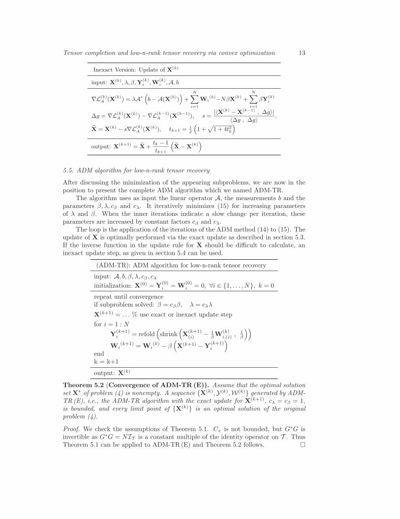
5.5. ADM algorithm for low-n-rank tensor recovery
After discussing the minimization of the appearing subproblems, we are now in theposition to present the complete ADM algorithm which we named ADM-TR.
The algorithm uses as input the linear operator A, the measurements b and theparameters β, λ, cβ and cλ. It iteratively minimizes (15) for increasing parametersof λ and β. When the inner iterations indicate a slow change per iteration, theseparameters are increased by constant factors cβ and cλ.
The loop is the application of the iterations of the ADM method (14) to (15). Theupdate of X is optimally performed via the exact update as described in section 5.3.If the inverse function in the update rule for X should be difficult to calculate, aninexact update step, as given in section 5.4 can be used.
(ADM-TR): ADM algorithm for low-n-rank tensor recovery
input: A, b, β, λ, cβ , cλinitialization: X(0) = Y
(0)i = W
(0)i = 0, ∀i ∈ 1, . . . , N, k = 0
repeat until convergenceif subproblem solved: β = cββ, λ = cλλ
X(k+1) = . . . % use exact or inexact update step
for i = 1 : N
Y(k+1)i = refold
(shrink
(X
(k+1)(i) − 1
βW
(k)i,(i) ,
1β
))
Wi(k+1) = Wi
(k) − β(X(k+1) −Y
(k+1)i
)
endk = k+1
output: X(k)
Theorem 5.2 (Convergence of ADM-TR (E)). Assume that the optimal solutionset X∗ of problem (4) is nonempty. A sequence X(k),Y(k),W(k) generated by ADM-TR (E), i.e., the ADM-TR algorithm with the exact update for X(k+1), cλ = cβ = 1,is bounded, and every limit point of X(k) is an optimal solution of the originalproblem (4).
Proof. We check the assumptions of Theorem 5.1. Cx is not bounded, but G∗G isinvertible as G∗G = NIT is a constant multiple of the identity operator on T . ThusTheorem 5.1 can be applied to ADM-TR (E) and Theorem 5.2 follows.
Tensor completion and low-n-rank tensor recovery via convex optimization 14
6. Numerical experiments
In this section, we evaluate the empirical performance of the proposed algorithms. Weperformed experiments in the tensor completion setup, where we first used randomlygenerated input data. We compared the results with other algorithms, namely LRTC(Low Rank Tensor Completion) [6] and the N-way toolbox for MATLAB. Then weapplied the algorithms to the completion of third-order tensors, taken from medicalimaging (MRI scans of parts of the human body) and hyperspectral data.
Remark: The computational cost of the algorithms DR-TR and ADM-TR relatesas follows to the size of n1, . . . , nN and the size of N . The sizes ni determinethe size of the unfolded tensors and thereby influence the computational cost ofone (partial) singular value decomposition which is the main operation within theshrinkage operator. A singular value decomposition of a matrix of dimensions n × nhas complexity O(n3) [20]. However, using the Lanczos algorithm for computingonly the singular vectors corresponding to the largest singular values speeds up thecalculation [28, 29]. The order N governs the number of different unfoldings ofthe tensor. In total there are N shrinkage operations applied per iteration of thealgorithms.
Experiments with randomly generated problem settings: In each experiment wegenerated a low-n-rank tensor X0 which we used as ground truth. Therefore, wefixed the dimension r of a ‘core tensor’ S ∈ R
r×...×r which we filled with Gaussiandistributed entries (∼ N (0, 1)). Then, we generated matrices Ψ(1), . . . ,Ψ(N), withΨ(i) ∈ R
ni×r and set
X0 := S ×1 Ψ(1) ×2 . . .×N Ψ(N).
With this construction, the n-rank of X0 equals (r, r, . . . , r) almost surely. We fixeda percentage ρs of the entries to be known and chose the support of the knownentries uniformly at random among all supports of size ρs
∏Ni=1 ni. The values and
the locations of the known entries of X0 was used as input for the algorithms.We used four different settings to test the algorithms. The order of the tensors
varied from three to five, and we also varied the n-rank and the fraction ρs of knownentries. Table 1 shows these different settings and the recovery performance fordifferent algorithms. The parameters were set to cβ = 2, cλ = 2, β = 1, λ = N, γ′ =1/β and tk = 1. We compared the ADM algorithm with inexact (ADM-TR (IE)) andexact (ADM-TR (E)) update rule for X, the Douglas-Rachford splitting for tensorrecovery (DR-TR) and the N-way toolbox for MATLAB.
The N-way toolbox for MATLAB fits a tensor of a given n-rank [r1, r2, . . . , rN ] tothe given input data TΩ, i.e., it essentially solves:
minimize ||XΩ −TΩ||F s. t. n-rank(X) = [r1, r2, . . . , rN ]
In table 1 we show the results for two different initializations of the N-waytoolbox. In N-way-E, we provided the exact n-rank of the ground-truth tensor X0
to the algorithm. As this is a very strong extra information, we also run the N-waytoolbox providing it an incorrect model information. In the setting N-way-IM, we toldthe toolbox to fit a tensor whose unfoldings have rank: rank(X(i)) = rank((X0)(i))+1.
The experiments in table 1 can be considered to vary from small-sized problemsto large-sized problems. Note that the number of entries of a tensor of dimensions20×20×20×20×20 has 205 = 3, 2 million entries. The computations were performed
Tensor completion and low-n-rank tensor recovery via convex optimization 15
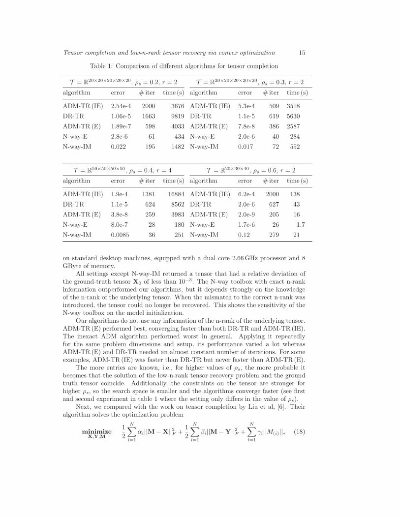
Table 1: Comparison of different algorithms for tensor completion
T = R20×20×20×20×20, ρs = 0.2, r = 2 T = R
20×20×20×20×20, ρs = 0.3, r = 2
algorithm error # iter time (s) algorithm error # iter time (s)
ADM-TR (IE) 2.54e-4 2000 3676 ADM-TR (IE) 5.3e-4 509 3518
DR-TR 1.06e-5 1663 9819 DR-TR 1.1e-5 619 5630
ADM-TR (E) 1.89e-7 598 4033 ADM-TR (E) 7.8e-8 386 2587
N-way-E 2.8e-6 61 434 N-way-E 2.0e-6 40 284
N-way-IM 0.022 195 1482 N-way-IM 0.017 72 552
T = R50×50×50×50, ρs = 0.4, r = 4 T = R
20×30×40, ρs = 0.6, r = 2
algorithm error # iter time (s) algorithm error # iter time (s)
ADM-TR (IE) 1.9e-4 1381 16884 ADM-TR (IE) 6.2e-4 2000 138
DR-TR 1.1e-5 624 8562 DR-TR 2.0e-6 627 43
ADM-TR (E) 3.8e-8 259 3983 ADM-TR (E) 2.0e-9 205 16
N-way-E 8.0e-7 28 180 N-way-E 1.7e-6 26 1.7
N-way-IM 0.0085 36 251 N-way-IM 0.12 279 21
on standard desktop machines, equipped with a dual core 2.66GHz processor and 8GByte of memory.
All settings except N-way-IM returned a tensor that had a relative deviation ofthe ground-truth tensor X0 of less than 10−3. The N-way toolbox with exact n-rankinformation outperformed our algorithms, but it depends strongly on the knowledgeof the n-rank of the underlying tensor. When the mismatch to the correct n-rank wasintroduced, the tensor could no longer be recovered. This shows the sensitivity of theN-way toolbox on the model initialization.
Our algorithms do not use any information of the n-rank of the underlying tensor.ADM-TR (E) performed best, converging faster than both DR-TR and ADM-TR (IE).The inexact ADM algorithm performed worst in general. Applying it repeatedlyfor the same problem dimensions and setup, its performance varied a lot whereasADM-TR (E) and DR-TR needed an almost constant number of iterations. For someexamples, ADM-TR (IE) was faster than DR-TR but never faster than ADM-TR (E).
The more entries are known, i.e., for higher values of ρs, the more probable itbecomes that the solution of the low-n-rank tensor recovery problem and the groundtruth tensor coincide. Additionally, the constraints on the tensor are stronger forhigher ρs, so the search space is smaller and the algorithms converge faster (see firstand second experiment in table 1 where the setting only differs in the value of ρs).
Next, we compared with the work on tensor completion by Liu et al, [6]. Theiralgorithm solves the optimization problem
minimizeX,Y,M
1
2
N∑
i=1
αi||M−X||2F +1
2
N∑
i=1
βi||M−Y||2F +N∑
i=1
γi||M(i)||∗ (18)
Tensor completion and low-n-rank tensor recovery via convex optimization 16
Table 2: Tensor recovery experiments with LRTC [6]
tensor dimensions ρ r # iter rel. error time(s)
T = R20×20×20×20×20 0.2 2
500 0.379 12632000 0.0198 3535
T = R20×20×20×20×20 0.3 2
500 0.489 12612000 0.034 3992
T = R50×50×50×50 0.4 4
500 0.613 22162000 0.021 6238
T = R20×30×40 0.6 2
500 0.0105 6.92000 0.168 26.5
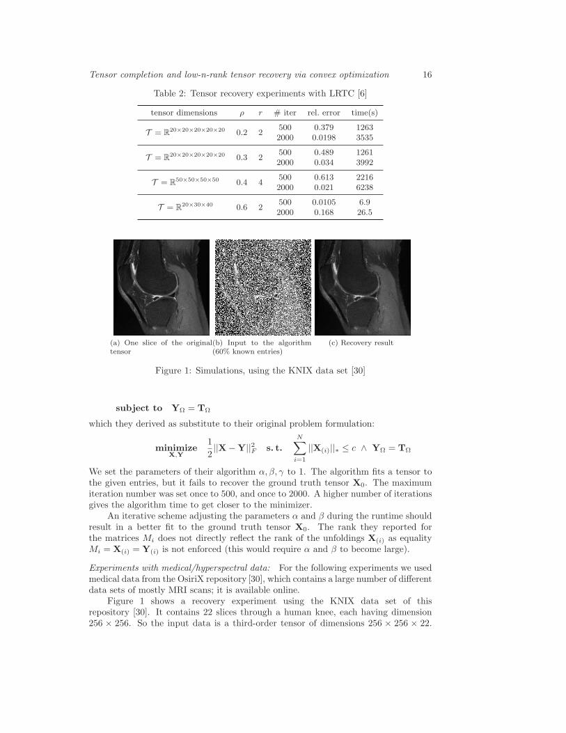
(a) One slice of the originaltensor
(b) Input to the algorithm(60% known entries)
(c) Recovery result
Figure 1: Simulations, using the KNIX data set [30]
subject to YΩ = TΩ
which they derived as substitute to their original problem formulation:
minimizeX,Y
1
2||X−Y||2F s. t.
N∑
i=1
||X(i)||∗ ≤ c ∧ YΩ = TΩ
We set the parameters of their algorithm α, β, γ to 1. The algorithm fits a tensor tothe given entries, but it fails to recover the ground truth tensor X0. The maximumiteration number was set once to 500, and once to 2000. A higher number of iterationsgives the algorithm time to get closer to the minimizer.
An iterative scheme adjusting the parameters α and β during the runtime shouldresult in a better fit to the ground truth tensor X0. The rank they reported forthe matrices Mi does not directly reflect the rank of the unfoldings X(i) as equalityMi = X(i) = Y(i) is not enforced (this would require α and β to become large).
Experiments with medical/hyperspectral data: For the following experiments we usedmedical data from the OsiriX repository [30], which contains a large number of differentdata sets of mostly MRI scans; it is available online.
Figure 1 shows a recovery experiment using the KNIX data set of thisrepository [30]. It contains 22 slices through a human knee, each having dimension256 × 256. So the input data is a third-order tensor of dimensions 256 × 256 × 22.
Tensor completion and low-n-rank tensor recovery via convex optimization 17
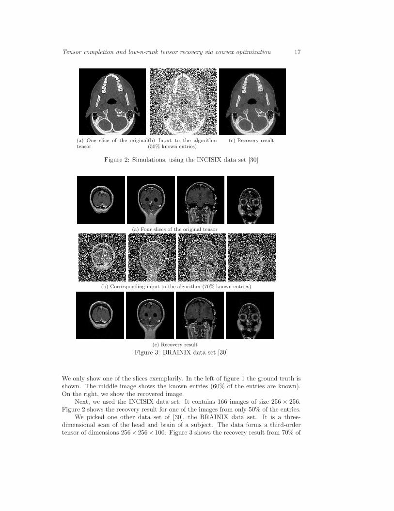
(a) One slice of the originaltensor
(b) Input to the algorithm(50% known entries)
(c) Recovery result
Figure 2: Simulations, using the INCISIX data set [30]
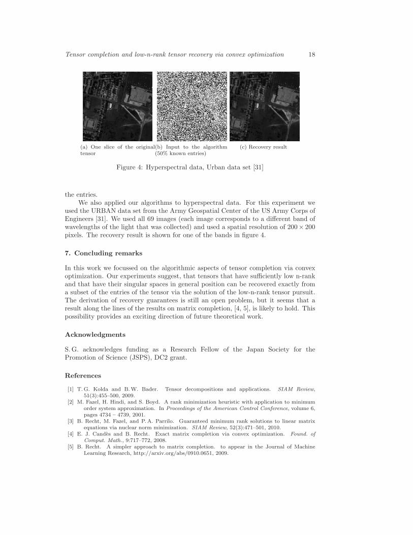
(a) Four slices of the original tensor
(b) Corresponding input to the algorithm (70% known entries)
(c) Recovery result
Figure 3: BRAINIX data set [30]
We only show one of the slices exemplarily. In the left of figure 1 the ground truth isshown. The middle image shows the known entries (60% of the entries are known).On the right, we show the recovered image.
Next, we used the INCISIX data set. It contains 166 images of size 256 × 256.Figure 2 shows the recovery result for one of the images from only 50% of the entries.
We picked one other data set of [30], the BRAINIX data set. It is a three-dimensional scan of the head and brain of a subject. The data forms a third-ordertensor of dimensions 256× 256× 100. Figure 3 shows the recovery result from 70% of
Tensor completion and low-n-rank tensor recovery via convex optimization 18
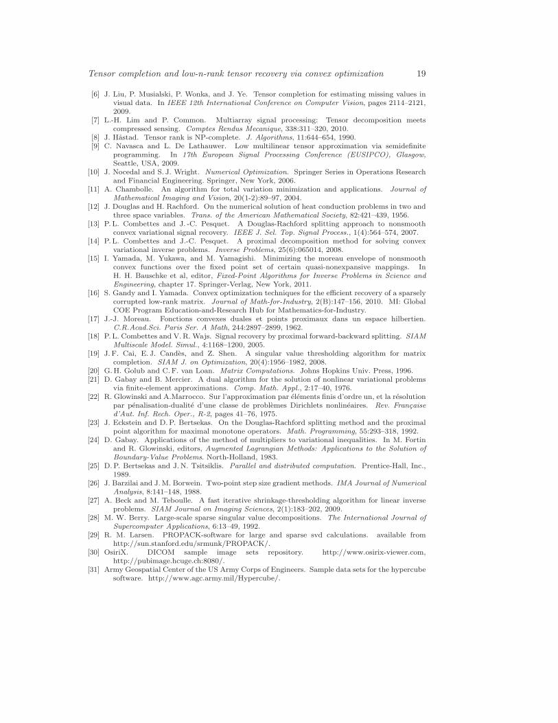
(a) One slice of the originaltensor
(b) Input to the algorithm(50% known entries)
(c) Recovery result
Figure 4: Hyperspectral data, Urban data set [31]
the entries.We also applied our algorithms to hyperspectral data. For this experiment we
used the URBAN data set from the Army Geospatial Center of the US Army Corps ofEngineers [31]. We used all 69 images (each image corresponds to a different band ofwavelengths of the light that was collected) and used a spatial resolution of 200× 200pixels. The recovery result is shown for one of the bands in figure 4.
7. Concluding remarks
In this work we focussed on the algorithmic aspects of tensor completion via convexoptimization. Our experiments suggest, that tensors that have sufficiently low n-rankand that have their singular spaces in general position can be recovered exactly froma subset of the entries of the tensor via the solution of the low-n-rank tensor pursuit.The derivation of recovery guarantees is still an open problem, but it seems that aresult along the lines of the results on matrix completion, [4, 5], is likely to hold. Thispossibility provides an exciting direction of future theoretical work.
Acknowledgments
S.G. acknowledges funding as a Research Fellow of the Japan Society for thePromotion of Science (JSPS), DC2 grant.
References
[1] T.G. Kolda and B.W. Bader. Tensor decompositions and applications. SIAM Review,51(3):455–500, 2009.
[2] M. Fazel, H. Hindi, and S. Boyd. A rank minimization heuristic with application to minimumorder system approximation. In Proceedings of the American Control Conference, volume 6,pages 4734 – 4739, 2001.
[3] B. Recht, M. Fazel, and P.A. Parrilo. Guaranteed minimum rank solutions to linear matrixequations via nuclear norm minimization. SIAM Review, 52(3):471–501, 2010.
[4] E. J. Candes and B. Recht. Exact matrix completion via convex optimization. Found. ofComput. Math., 9:717–772, 2008.
[5] B. Recht. A simpler approach to matrix completion. to appear in the Journal of MachineLearning Research, http://arxiv.org/abs/0910.0651, 2009.
Tensor completion and low-n-rank tensor recovery via convex optimization 19
[6] J. Liu, P. Musialski, P. Wonka, and J. Ye. Tensor completion for estimating missing values invisual data. In IEEE 12th International Conference on Computer Vision, pages 2114–2121,2009.
[7] L.-H. Lim and P. Common. Multiarray signal processing: Tensor decomposition meetscompressed sensing. Comptes Rendus Mecanique, 338:311–320, 2010.
[8] J. Hastad. Tensor rank is NP-complete. J. Algorithms, 11:644–654, 1990.[9] C. Navasca and L. De Lathauwer. Low multilinear tensor approximation via semidefinite
programming. In 17th European Signal Processing Conference (EUSIPCO), Glasgow,Seattle, USA, 2009.
[10] J. Nocedal and S. J. Wright. Numerical Optimization. Springer Series in Operations Researchand Financial Engineering. Springer, New York, 2006.
[11] A. Chambolle. An algorithm for total variation minimization and applications. Journal ofMathematical Imaging and Vision, 20(1-2):89–97, 2004.
[12] J. Douglas and H. Rachford. On the numerical solution of heat conduction problems in two andthree space variables. Trans. of the American Mathematical Society, 82:421–439, 1956.
[13] P. L. Combettes and J. -C. Pesquet. A Douglas-Rachford splitting approach to nonsmoothconvex variational signal recovery. IEEE J. Sel. Top. Signal Process., 1(4):564–574, 2007.
[14] P. L. Combettes and J.-C. Pesquet. A proximal decomposition method for solving convexvariational inverse problems. Inverse Problems, 25(6):065014, 2008.
[15] I. Yamada, M. Yukawa, and M. Yamagishi. Minimizing the moreau envelope of nonsmoothconvex functions over the fixed point set of certain quasi-nonexpansive mappings. InH. H. Bauschke et al, editor, Fixed-Point Algorithms for Inverse Problems in Science andEngineering, chapter 17. Springer-Verlag, New York, 2011.
[16] S. Gandy and I. Yamada. Convex optimization techniques for the efficient recovery of a sparselycorrupted low-rank matrix. Journal of Math-for-Industry, 2(B):147–156, 2010. MI: GlobalCOE Program Education-and-Research Hub for Mathematics-for-Industry.
[17] J.-J. Moreau. Fonctions convexes duales et points proximaux dans un espace hilbertien.C.R.Acad.Sci. Paris Ser. A Math, 244:2897–2899, 1962.
[18] P. L. Combettes and V.R. Wajs. Signal recovery by proximal forward-backward splitting. SIAMMultiscale Model. Simul., 4:1168–1200, 2005.
[19] J. F. Cai, E. J. Candes, and Z. Shen. A singular value thresholding algorithm for matrixcompletion. SIAM J. on Optimization, 20(4):1956–1982, 2008.
[20] G.H. Golub and C.F. van Loan. Matrix Computations. Johns Hopkins Univ. Press, 1996.[21] D. Gabay and B. Mercier. A dual algorithm for the solution of nonlinear variational problems
via finite-element approximations. Comp. Math. Appl., 2:17–40, 1976.[22] R. Glowinski and A.Marrocco. Sur l’approximation par elements finis d’ordre un, et la resolution
par penalisation-dualite d’une classe de problemes Dirichlets nonlineaires. Rev. Francaised’Aut. Inf. Rech. Oper., R-2, pages 41–76, 1975.
[23] J. Eckstein and D.P. Bertsekas. On the Douglas-Rachford splitting method and the proximalpoint algorithm for maximal monotone operators. Math. Programming, 55:293–318, 1992.
[24] D. Gabay. Applications of the method of multipliers to variational inequalities. In M. Fortinand R. Glowinski, editors, Augmented Lagrangian Methods: Applications to the Solution ofBoundary-Value Problems. North-Holland, 1983.
[25] D. P. Bertsekas and J.N. Tsitsiklis. Parallel and distributed computation. Prentice-Hall, Inc.,1989.
[26] J. Barzilai and J.M. Borwein. Two-point step size gradient methods. IMA Journal of NumericalAnalysis, 8:141–148, 1988.
[27] A. Beck and M. Teboulle. A fast iterative shrinkage-thresholding algorithm for linear inverseproblems. SIAM Journal on Imaging Sciences, 2(1):183–202, 2009.
[28] M. W. Berry. Large-scale sparse singular value decompositions. The International Journal ofSupercomputer Applications, 6:13–49, 1992.
[29] R. M. Larsen. PROPACK-software for large and sparse svd calculations. available fromhttp://sun.stanford.edu/srmunk/PROPACK/.
[30] OsiriX. DICOM sample image sets repository. http://www.osirix-viewer.com,http://pubimage.hcuge.ch:8080/.
[31] Army Geospatial Center of the US Army Corps of Engineers. Sample data sets for the hypercubesoftware. http://www.agc.army.mil/Hypercube/.