Embed Size (px)
Citation preview

On Tensor Completion via Nuclear Norm Minimization
Ming Yuan∗ and Cun-Hui Zhang†
University of Wisconsin-Madison and Rutgers University
(April 21, 2015)
Abstract
Many problems can be formulated as recovering a low-rank tensor. Although an
increasingly common task, tensor recovery remains a challenging problem because
of the delicacy associated with the decomposition of higher order tensors. To
overcome these difficulties, existing approaches often proceed by unfolding tensors
into matrices and then apply techniques for matrix completion. We show here that
such matricization fails to exploit the tensor structure and may lead to suboptimal
procedure. More specifically, we investigate a convex optimization approach to tensor
completion by directly minimizing a tensor nuclear norm and prove that this leads to
an improved sample size requirement. To establish our results, we develop a series
of algebraic and probabilistic techniques such as characterization of subdifferetial for
tensor nuclear norm and concentration inequalities for tensor martingales, which may
be of independent interests and could be useful in other tensor related problems.
∗Department of Statistics, University of Wisconsin-Madison, Madison, WI 53706. The research of Ming
Yuan was supported in part by NSF Career Award DMS-1321692 and FRG Grant DMS-1265202, and NIH
Grant 1U54AI117924-01.†Department of Statistics and Biostatistics, Rutgers University, Piscataway, New Jersey 08854. The
research of Cun-Hui Zhang was supported in part by NSF Grants DMS-1129626 and DMS-1209014
1
1 Introduction
Let T ∈ Rd1×d2×···×dN be an Nth order tensor, and Ω be a randomly sampled subset of
[d1]×· · ·× [dN ] where [d] = 1, 2, . . . , d. The goal of tensor completion is to recover T when
observing only entries T (ω) for ω ∈ Ω. In particular, we are interested in the case when
the dimensions d1, . . . , dN are large. Such a problem arises naturally in many applications.
Examples include hyper-spectral image analysis (Li and Li, 2010), multi-energy computed
tomography (Semerci et al., 2013), radar signal processing (Sidiropoulos and Nion, 2010),
audio classification (Mesgarani, Slaney and Shamma, 2006) and text mining (Cohen and
Collins, 2012) among numerous others. Common to these and many other problems, the
tensor T can oftentimes be identified with a certain low-rank structure. The low-rankness
entails reduction in degrees of freedom, and as a result, it is possible to recover T exactly
even when the sample size |Ω| is much smaller than the total number, d1d2 · · · dN , of entriesin T .
In particular, when N = 2, this becomes the so-called matrix completion problem which
has received considerable amount of attention in recent years. See, e.g., Candes and Recht
(2008), Candes and Tao (2009), Recht (2010), and Gross (2011) among many others. An
especially attractive approach is through nuclear norm minimization:
minX∈Rd1×d2
∥X∥∗ subject to X(ω) = T (ω) ∀ω ∈ Ω,
where the nuclear norm ∥ · ∥∗ of a matrix is given by
∥X∥∗ =mind1,d2∑
k=1
σk(X),
and σk(·) stands for the kth largest singular value of a matrix. Denote by T the solution to
the aforementioned nuclear norm minimization problem. As shown, for example, by Gross
(2011), if an unknown d1 × d2 matrix T of rank r is of low coherence with respect to the
canonical basis, then it can be perfectly reconstructed by T with high probability whenever
|Ω| ≥ C(d1 + d2)r log2(d1 + d2), where C is a numerical constant. In other words, perfect
recovery of a matrix is possible with observations from a very small fraction of entries in T .
In many practical situations, we need to consider higher order tensors. The seemingly
innocent task of generalizing these ideas from matrices to higher order tensor completion
problems, however, turns out to be rather subtle, as basic notion such as rank, or singular
value decomposition, becomes ambiguous for higher order tensors (e.g., Kolda and Bader,
2009; Hillar and Lim, 2013). A common strategy to overcome the challenges in dealing
with high order tensors is to unfold them to matrices, and then resort to the usual nuclear
2
norm minimization heuristics for matrices. To fix ideas, we shall focus on third order tensors
(N = 3) in the rest of the paper although our techniques can be readily used to treat higher
order tensor. Following the matricization approach, T can be reconstructed by the solution
of the following convex program:
minX∈Rd1×d2×d3
∥X(1)∥∗ + ∥X(2)∥∗ + ∥X(3)∥∗ subject to X(ω) = T (ω) ∀ω ∈ Ω,
where X(j) is a dj × (∏
k =j dk) matrix whose columns are the mode-j fibers of X. See,
e.g., Liu et al. (2009), Signoretto, Lathauwer and Suykens (2010), Gandy et al. (2011),
Tomioka, Hayashi and Kashima (2010), and Tomioka et al. (2011). In the light of existing
results on matrix completion, with this approach, T can be reconstructed perfectly with
high probability provided that
|Ω| ≥ C(d1d2r3 + d1r2d3 + r1d2d3) log2(d1 + d2 + d3)
uniformly sampled entries are observed, where rj is the rank of X(j) and C is a numerical
constant. See, e.g., Mu et al. (2013). It is of great interests to investigate if this sample
size requirement can be improved by avoiding matricization of tensors. We show here that
the answer indeed is affirmative and a more direct nuclear norm minimization formulation
requires a smaller sample size to recover T .
More specifically, write, for two tensors X,Y ∈ Rd1×d2×d3 ,
⟨X,Y ⟩ =∑
ω∈[d1]×[d2]×[d3]
X(ω)Y (ω)
as their inner product. Define
∥X∥ = maxuj∈Rdj :∥u1∥=∥u2∥=∥u3∥=1
⟨X,u1 ⊗ u2 ⊗ u3⟩,
where, with slight abuse of notation, ∥ · ∥ also stands for the usual Euclidean norm for a
vector, and for vectors uj = (uj1, . . . , u
jdj)⊤,
u1 ⊗ u2 ⊗ u3 = (u1au
2bu
3c)1≤a≤d1,1≤b≤d2,1≤c≤d3 .
It is clear that the ∥·∥ defined above for tensors is a norm and can be viewed as an extension
of the usual matrix spectral norm. Appealing to the duality between the spectral norm and
nuclear norm in the matrix case, we now consider the following nuclear norm for tensors:
∥X∥∗ = maxY ∈Rd1×d2×d3 :∥Y ∥≤1
⟨Y ,X⟩.
3
It is clear that ∥ · ∥∗ is also a norm. We then consider reconstructing T via the solution to
the following convex program:
minX∈Rd1×d2×d3
∥X∥∗ subject to X(ω) = T (ω) ∀ω ∈ Ω.
We show that the sample size requirement for perfect recovery of a tensor with low coherence
using this approach is
|Ω| ≥ C(r2(d1 + d2 + d3) +
√rd1d2d3
)polylog (d1 + d2 + d3) ,
where
r =√
(r1r2d3 + r1r3d2 + r2r3d1)/(d1 + d2 + d3),
polylog(x) is a certain polynomial function of log(x), and C is a numerical constant. In
particular, when considering (nearly) cubic tensors with d1, d2 and d3 approximately equal
to a common d, then this sample size requirement is essentially of the order r1/2(d log d)3/2.
In the case when the tensor dimension d is large while the rank r is relatively small, this can
be a drastic improvement over the existing results based on matricizing tensors where the
sample size requirement is r(d log d)2.
The high-level strategy to the investigation of the proposed nuclear norm minimization
approach for tensors is similar, in a sense, to the treatment of matrix completion. Yet
the analysis for tensors is much more delicate and poses significant new challenges because
many of the well-established tools for matrices, either algebraic such as characterization of
the subdifferential of the nuclear norm, or probabilistic such as concentration inequalities
for martingales, do not exist for tensors. Some of these disparities can be bridged and we
develop various tools to do so. Others are due to fundamental differences between matrices
and higher order tensors, and we devise new strategies to overcome them. The tools and
techniques we developed may be of independent interests and can be useful in dealing with
other problems for tensors.
The rest of the paper is organized as follows. We first describe some basic properties of
tensors and their nuclear norm necessary for our analysis in Section 2. Section 3 discusses
the main architect of our analysis. The main probabilistic tools we use are concentration
bounds for the sum of random tensors. Because the tensor spectral norm does not have the
interpretation as an operator norm of a linear mapping between Hilbert spaces, the usual
matrix Bernstein inequality cannot be directly applied. It turns out that different strategies
are required for tensors of low rank and tensors with sparse support, and these results are
presented in Sections 4 and 5 respectively. We conclude the paper with a few remarks in
Section 6.
4
2 Tensor
We first collect some useful algebraic facts for tensors essential to our later analysis. Recall
that the inner product between two third order tensors X,Y ∈ Rd1×d2×d3 is given by
⟨X,Y ⟩ =d1∑a=1
d2∑b=1
d3∑c=1
X(a, b, c)Y (a, b, c),
and ∥X∥HS = ⟨X,X⟩1/2 is the usual Hilbert-Schmidt norm of X. Another tensor norm of
interest is the entrywise ℓ∞ norm, or tensor max norm:
∥X∥max = maxω∈[d1]×[d2]×[d3]
|X(ω)|.
It is clear that for any the third order tensor X ∈ Rd1×d2×d3 ,
∥X∥max ≤ ∥X∥ ≤ ∥X∥HS ≤ ∥X∥∗, and ∥X∥2HS ≤ ∥X∥∗∥X∥.
We shall also encounter linear maps defined on tensors. Let R : Rd1×d2×d3 → Rd1×d2×d3
be a linear map. We define the induced operator norm of R under tensor Hilbert-Schmidt
norm as
∥R∥ = max∥RX∥HS : X ∈ Rd1×d2×d3 , ∥X∥HS ≤ 1
.
2.1 Decomposition and Projection
Consider the following tensor decomposition of X into rank-one tensors:
X = [A,B,C] :=r∑
k=1
ak ⊗ bk ⊗ ck, (1)
where aks, bks and cks are the column vectors of matrices A, B and C respectively. Such a
decomposition in general is not unique (see, e.g., Kruskal, 1989). However, the linear spaces
spanned by columns of A, B and C respectively are uniquely defined.
More specifically, write X(·, b, c) = (X(1, b, c), . . . ,X(d1, b, c))⊤, that is the mode-1 fiber
of X. Define X(a, ·, c) and X(a, b, ·) in a similar fashion. Let
L1(X) = l.s.X(·, b, c) : 1 ≤ b ≤ d2, 1 ≤ c ≤ d3;L2(X) = l.s.X(a, ·, c) : 1 ≤ a ≤ d1, 1 ≤ c ≤ d3;L3(X) = l.s.X(a, b, ·) : 1 ≤ a ≤ d1, 1 ≤ b ≤ d2,
where l.s. represents the linear space spanned by a collection of vectors of conformable
dimension. Then it is clear that the linear space spanned by the column vectors of A is
5
L1(X), and similar statements hold true for the column vectors of B and C. In the case of
matrices, both marginal linear spaces, L1 and L2 are necessarily of the same dimension as
they are spanned by the respective singular vectors. For higher order tensors, however, this
is typically not true. We shall denote by rj(X) the dimension of Lj(X) for j = 1, 2 and 3,
which are often referred to the Tucker ranks of X. Another useful notion of “tensor rank”
for our purposes is
r(X) =√
(r1(X)r2(X)d3 + r1(X)r3(X)d2 + r2(X)r3(X)d1) /d.
where d = d1 + d2 + d3, which can also be viewed as a generalization of the matrix rank to
tensors. It is well known that the smallest value for r in the rank-one decomposition (1) is
in [r(X), r2(X)]. See, e.g., Kolda and Bader (2009).
Let M be a matrix of size d0 × d1. Marginal multiplication of M and a tensor X in the
first coordinate yields a tensor of size d0 × d2 × d3:
(M ×1 X)(a, b, c) =
d1∑a′=1
Maa′X(a′, b, c).
It is easy to see that if X = [A,B,C], then M×1X = [MA,B,C]. Marginal multiplications
×2 and ×3 between a matrix of conformable size and X can be similarly defined.
Let P be arbitrary projection from Rd1 to a linear subspace of Rd1 . It is clear from
the definition of marginal multiplications, [PA,B,C] is also uniquely defined for tensor
X = [A,B,C], that is, [PA,B,C] does not depend on the particular decomposition of A,
B, C. Now let P j be arbitrary projection from Rdj to a linear subspace of Rdj . Define a
tensor projection P 1 ⊗ P 2 ⊗ P 3 on X = [A,B,C] as
(P 1 ⊗ P 2 ⊗ P 3)X = [P 1A,P 2B,P 3C].
We note that there is no ambiguity in defining (P 1 ⊗P 2 ⊗P 3)X because of the uniqueness
of marginal projections.
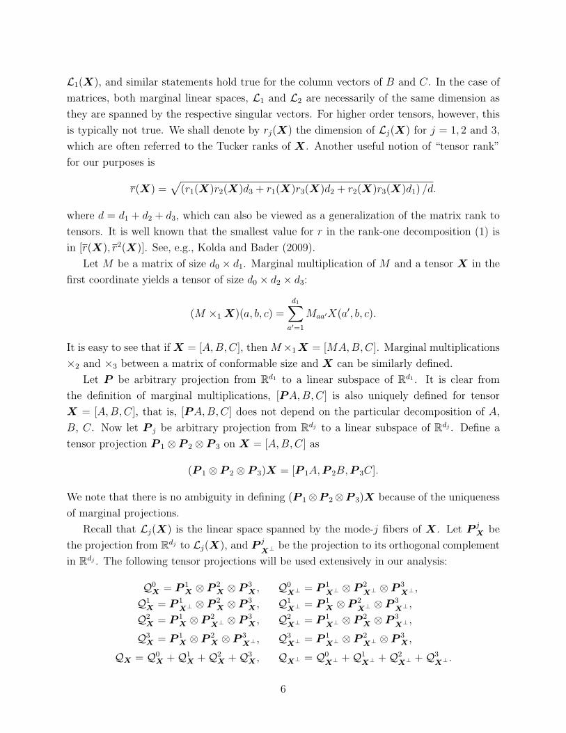
Recall that Lj(X) is the linear space spanned by the mode-j fibers of X. Let P jX be
the projection from Rdj to Lj(X), and P j
X⊥ be the projection to its orthogonal complement
in Rdj . The following tensor projections will be used extensively in our analysis:
Q0X = P 1
X ⊗ P 2X ⊗ P 3
X , Q0X⊥ = P 1
X⊥ ⊗ P 2X⊥ ⊗ P 3
X⊥ ,
Q1X = P 1
X⊥ ⊗ P 2X ⊗ P 3
X , Q1X⊥ = P 1
X ⊗ P 2X⊥ ⊗ P 3
X⊥ ,
Q2X = P 1
X ⊗ P 2X⊥ ⊗ P 3
X , Q2X⊥ = P 1
X⊥ ⊗ P 2X ⊗ P 3
X⊥ ,
Q3X = P 1
X ⊗ P 2X ⊗ P 3
X⊥ , Q3X⊥ = P 1
X⊥ ⊗ P 2X⊥ ⊗ P 3
X ,
QX = Q0X +Q1
X +Q2X +Q3
X , QX⊥ = Q0X⊥ +Q1
X⊥ +Q2X⊥ +Q3
X⊥ .
6
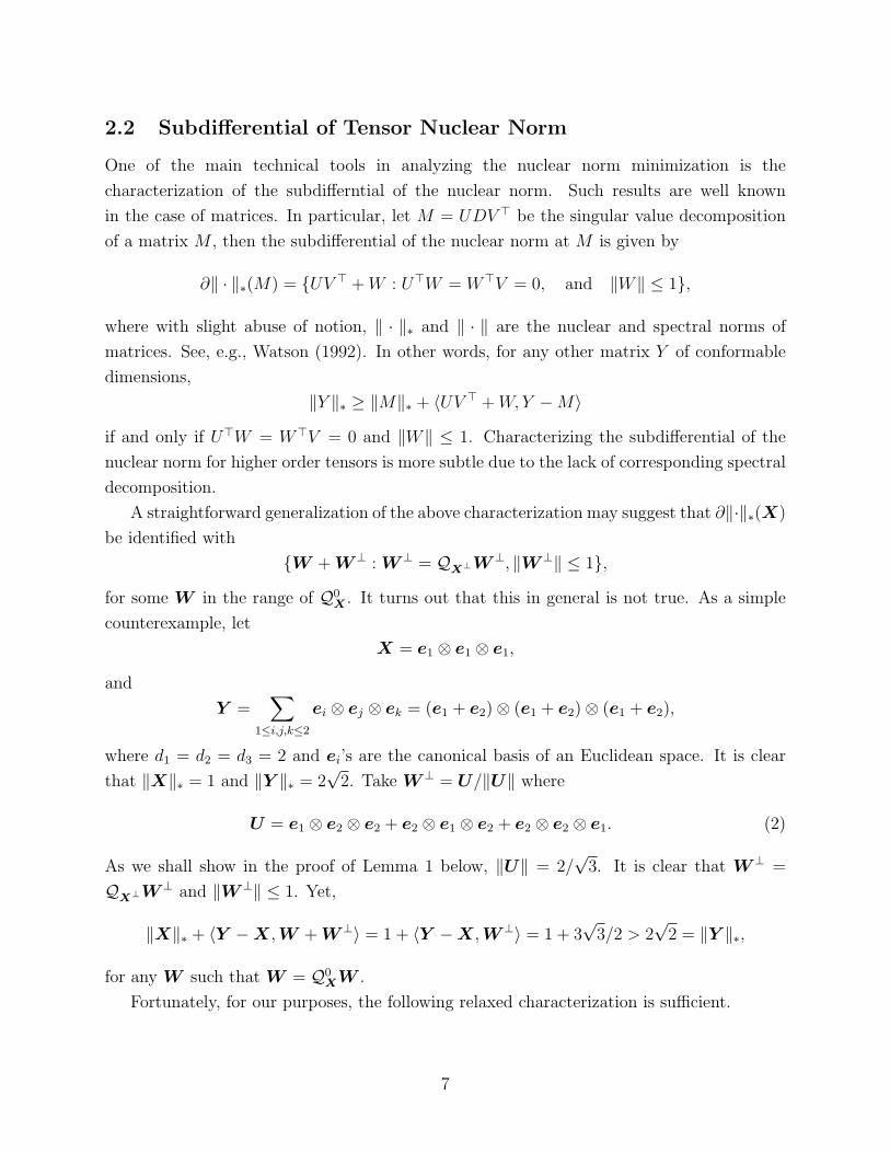
2.2 Subdifferential of Tensor Nuclear Norm
One of the main technical tools in analyzing the nuclear norm minimization is the
characterization of the subdifferntial of the nuclear norm. Such results are well known
in the case of matrices. In particular, let M = UDV ⊤ be the singular value decomposition
of a matrix M , then the subdifferential of the nuclear norm at M is given by
∂∥ · ∥∗(M) = UV ⊤ +W : U⊤W = W⊤V = 0, and ∥W∥ ≤ 1,
where with slight abuse of notion, ∥ · ∥∗ and ∥ · ∥ are the nuclear and spectral norms of
matrices. See, e.g., Watson (1992). In other words, for any other matrix Y of conformable
dimensions,
∥Y ∥∗ ≥ ∥M∥∗ + ⟨UV ⊤ +W,Y −M⟩
if and only if U⊤W = W⊤V = 0 and ∥W∥ ≤ 1. Characterizing the subdifferential of the
nuclear norm for higher order tensors is more subtle due to the lack of corresponding spectral
decomposition.
A straightforward generalization of the above characterization may suggest that ∂∥·∥∗(X)
be identified with
W +W⊥ : W⊥ = QX⊥W⊥, ∥W⊥∥ ≤ 1,
for some W in the range of Q0X . It turns out that this in general is not true. As a simple
counterexample, let
X = e1 ⊗ e1 ⊗ e1,
and
Y =∑
1≤i,j,k≤2
ei ⊗ ej ⊗ ek = (e1 + e2)⊗ (e1 + e2)⊗ (e1 + e2),
where d1 = d2 = d3 = 2 and ei’s are the canonical basis of an Euclidean space. It is clear
that ∥X∥∗ = 1 and ∥Y ∥∗ = 2√2. Take W⊥ = U/∥U∥ where
U = e1 ⊗ e2 ⊗ e2 + e2 ⊗ e1 ⊗ e2 + e2 ⊗ e2 ⊗ e1. (2)
As we shall show in the proof of Lemma 1 below, ∥U∥ = 2/√3. It is clear that W⊥ =
QX⊥W⊥ and ∥W⊥∥ ≤ 1. Yet,
∥X∥∗ + ⟨Y −X,W +W⊥⟩ = 1 + ⟨Y −X,W⊥⟩ = 1 + 3√3/2 > 2
√2 = ∥Y ∥∗,
for any W such that W = Q0XW .
Fortunately, for our purposes, the following relaxed characterization is sufficient.
7

Lemma 1 For any third order tensor X ∈ Rd1×d2×d3, there exists a W ∈ Rd1×d2×d3 such
that W = Q0XW , ∥W ∥ = 1 and
∥X∥∗ = ⟨W ,X⟩.
Furthermore, for any Y ∈ Rd1×d2×d3 and W⊥ ∈ Rd1×d2×d3 obeying ∥W⊥∥ ≤ 1/2,
∥Y ∥∗ ≥ ∥X∥∗ + ⟨W +QX⊥W⊥,Y −X⟩.
Proof of Lemma 1. If ∥W ∥ ≤ 1, then
max∥uj∥=1
⟨Q0XW ,u1 ⊗ u2 ⊗ u3⟩ ≤ max
∥uj∥=1⟨W , (P 1
Xu1)⊗ (P 2Xu2)⊗ (P 3
Xu3)⟩ ≤ 1.
It follows that
∥X∥∗ = max∥W ∥=1
⟨W ,X⟩ = max∥W ∥=1
⟨Q0XW ,X⟩
is attained with a certain W satisfying ∥W ∥ = ∥Q0XW ∥ = 1.
Now consider a tensor W⊥ satisfying
∥W +QX⊥W⊥∥ ≤ 1.
Because QX⊥X = 0, it follows from the definition of the tensor nuclear norm that
⟨W +QX⊥W⊥,Y −X⟩ ≤ ∥Y ∥∗ − ⟨W ,X⟩ = ∥Y ∥∗ − ∥X∥∗.
It remains to prove that ∥W⊥∥ ≤ 1/2 implies
∥W +QX⊥W⊥∥ ≤ 1.
Recall that W = Q0XW , ∥W⊥∥ ≤ 1/2, and ∥uj∥ = 1. Then
⟨W +QX⊥W⊥,u1 ⊗ u2 ⊗ u3⟩≤ ∥Q0
X(u1 ⊗ u2 ⊗ u3)∥∗ +1
2∥QX⊥(u1 ⊗ u2 ⊗ u3)∥∗
≤3∏
j=1
√1− a2j +
1
2
(a1a2 + a1a3
√1− a22 + a2a3
√1− a21
).
where aj = ∥P j
X⊥uj∥2, for j = 1, 2, 3. Let x = a1a2 and
y =√(1− a21)(1− a22).
8
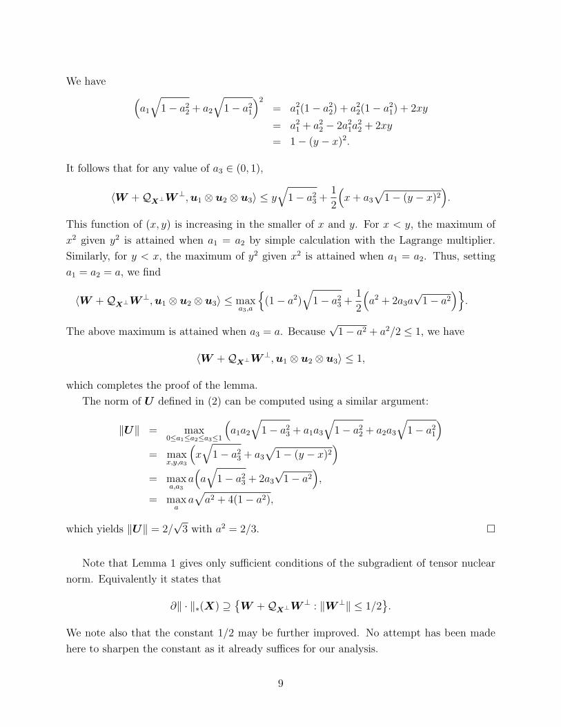
We have (a1
√1− a22 + a2
√1− a21
)2= a21(1− a22) + a22(1− a21) + 2xy
= a21 + a22 − 2a21a22 + 2xy
= 1− (y − x)2.
It follows that for any value of a3 ∈ (0, 1),
⟨W +QX⊥W⊥,u1 ⊗ u2 ⊗ u3⟩ ≤ y√
1− a23 +1
2
(x+ a3
√1− (y − x)2
).
This function of (x, y) is increasing in the smaller of x and y. For x < y, the maximum of
x2 given y2 is attained when a1 = a2 by simple calculation with the Lagrange multiplier.
Similarly, for y < x, the maximum of y2 given x2 is attained when a1 = a2. Thus, setting
a1 = a2 = a, we find
⟨W +QX⊥W⊥,u1 ⊗ u2 ⊗ u3⟩ ≤ maxa3,a
(1− a2)
√1− a23 +
1
2
(a2 + 2a3a
√1− a2
).
The above maximum is attained when a3 = a. Because√1− a2 + a2/2 ≤ 1, we have
⟨W +QX⊥W⊥,u1 ⊗ u2 ⊗ u3⟩ ≤ 1,
which completes the proof of the lemma.
The norm of U defined in (2) can be computed using a similar argument:
∥U∥ = max0≤a1≤a2≤a3≤1
(a1a2
√1− a23 + a1a3
√1− a22 + a2a3
√1− a21
)= max
x,y,a3
(x√
1− a23 + a3√
1− (y − x)2)
= maxa,a3
a(a√
1− a23 + 2a3√1− a2
),
= maxa
a√a2 + 4(1− a2),
which yields ∥U∥ = 2/√3 with a2 = 2/3.
Note that Lemma 1 gives only sufficient conditions of the subgradient of tensor nuclear
norm. Equivalently it states that
∂∥ · ∥∗(X) ⊇W +QX⊥W⊥ : ∥W⊥∥ ≤ 1/2
.
We note also that the constant 1/2 may be further improved. No attempt has been made
here to sharpen the constant as it already suffices for our analysis.
9
2.3 Coherence
A central concept to matrix completion is coherence. Recall that the coherence of an r
dimensional linear subspace U of Rk is defined as
µ(U) =k
rmax1≤i≤k
∥P Uei∥2 =max1≤i≤k ∥P Uei∥2
k−1∑k
i=1 ∥P Uei∥2,
where P U is the orthogonal projection onto U and ei’s are the canonical basis for Rk. See,
e.g., Candes and Recht (2008). We shall define the coherence of a tensor X ∈ Rd1×d2×d3 as
µ(X) = maxµ(L1(X)), µ(L2(X)), µ(L3(X)).
It is clear that µ(X) ≥ 1, since µ(U) is the ratio of the ℓ∞ and length-normalized ℓ2 norms
of a vector.
Lemma 2 Let X ∈ Rd1×d2×d3 be a third order tensor. Then
maxa,b,c
∥QX(ea ⊗ eb ⊗ ec)∥2HS ≤ r2(X)d
d1d2d3µ2(X).
Proof of Lemma 2. Recall that QX = Q0X +Q1
X +Q2X +Q3
X . Therefore,
∥QX(ea ⊗ eb ⊗ ec)∥2 =3∑
j,k=0
⟨QjX(ea ⊗ eb ⊗ ec),Qk
X(ea ⊗ eb ⊗ ec)⟩
=3∑
j=0
∥QjX(ea ⊗ eb ⊗ ec)∥2
= ∥P 1Xea∥2∥P 2
Xeb∥2∥P 3Xec∥2 + ∥P 1
X⊥ea∥2∥P 2Xeb∥2∥P 3
Xec∥2
+∥P 1Xea∥2∥P 2
X⊥eb∥2∥P 3Xec∥2 + ∥P 1
Xea∥2∥P 2Xeb∥2∥P 3
X⊥ec∥2.
For brevity, write rj = rj(X), and µ = µ(X). Then
∥P 1Xea∥2∥P 2
Xeb∥2∥P 3Xec∥2 + ∥P 1
X⊥ea∥2∥P 2Xeb∥2∥P 3
Xec∥2 ≤ r2r3µ2
d2d3;
∥P 1Xea∥2∥P 2
Xeb∥2∥P 3Xec∥2 + ∥P 1
Xea∥2∥P 2X⊥eb∥2∥P 3
Xec∥2 ≤ r1r3µ2
d1d3;
∥P 1Xea∥2∥P 2
Xeb∥2∥P 3Xec∥2 + ∥P 1
Xea∥2∥P 2Xeb∥2∥P 3
X⊥ec∥2 ≤ r1r2µ2
d1d2.
As a result, for any (a, b, c) ∈ [d1]× [d2]× [d3],
∥QX(ea ⊗ eb ⊗ ec)∥2 ≤µ2(r1r2d3 + r1d2r3 + d1r2r3)
d1d2d3,
10
which implies the desired statement.
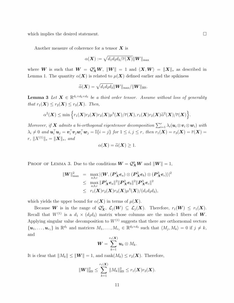
Another measure of coherence for a tensor X is
α(X) :=√d1d2d3/r(X)∥W ∥max
where W is such that W = Q0XW , ∥W ∥ = 1 and ⟨X,W ⟩ = ∥X∥∗ as described in
Lemma 1. The quantity α(X) is related to µ(X) defined earlier and the spikiness
α(X) =√
d1d2d3∥W ∥max/∥W ∥HS.
Lemma 3 Let X ∈ Rd1×d2×d3 be a third order tensor. Assume without loss of generality
that r1(X) ≤ r2(X) ≤ r3(X). Then,
α2(X) ≤ minr1(X)r2(X)r3(X)µ3(X)/r(X), r1(X)r2(X)α2(X)/r(X)
.
Moreover, if X admits a bi-orthogonal eigentensor decomposition∑r
i=1 λi(ui⊗vi⊗wi) with
λi = 0 and u⊤i uj = v⊤
i vjw⊤i wj = Ii = j for 1 ≤ i, j ≤ r, then r1(X) = r3(X) = r(X) =
r, ∥X(1)∥∗ = ∥X∥∗, andα(X) = α(X) ≥ 1.
Proof of Lemma 3. Due to the conditions W = Q0XW and ∥W ∥ = 1,
∥W ∥2max = maxa,b,c
|⟨W , (P 1Xea)⊗ (P 2
Xeb)⊗ (P 3Xec)⟩|2
≤ maxa,b,c
∥P 1Xea∥2∥P 2
Xeb∥2∥P 3Xec∥2
≤ r1(X)r2(X)r3(X)µ3(X)/(d1d2d3),
which yields the upper bound for α(X) in terms of µ(X).
Because W is in the range of Q0X , Lj(W ) ⊆ Lj(X). Therefore, r1(W ) ≤ r1(X).
Recall that W (1) is a d1 × (d2d3) matrix whose columns are the mode-1 fibers of W .
Applying singular value decomposition to W (1) suggests that there are orthornomal vectors
u1, . . . ,ur1 in Rd1 and matrices M1, . . . ,Mr1 ∈ Rd2×d3 such that ⟨Mj,Mk⟩ = 0 if j = k,
and
W =
r1(X)∑k=1
uk ⊗Mk.
It is clear that ∥Mk∥ ≤ ∥W ∥ = 1, and rank(Mk) ≤ r2(X). Therefore,
∥W ∥2HS ≤r1(X)∑k=1
∥Mk∥2HS ≤ r1(X)r2(X).
11

This gives the upper bound for α(X) in terms of α(X).
It remains to consider the case of X =∑r
i=1 λi(ui ⊗ vi ⊗wi). Obviously, by triangular
inequality,
∥X∥∗ ≤r∑
i=1
∥ui ⊗ vi ⊗wi∥∗ =r∑
i=1
∥wi∥.
On the other hand, let
W =r∑
i=1
ui ⊗ vi ⊗ (wi/∥wi∥).
Because
∥W ∥ ≤ maxa,b,c:∥a∥,∥b∥,∥c∥≤1
n∑i=1
∣∣∣(a⊤ui
)trace(cb⊤viw
⊤i /∥wi∥)
∣∣∣ ≤ ∥a∥∥bc⊤∥HS ≤ 1,
we find
∥X∥∗ ≥ ⟨W ,X⟩ =r∑
i=1
∥wi∥,
which implies that W is dual to X and
∥X∥∗ =r∑
i=1
∥wi∥,
where the rightmost hand side also equals to ∥X(1)∥∗ and ∥X(2)∥∗. The last statement now
follows from the fact that ∥W ∥2HS = r.
As in the matrix case, exact recovery with observations on a small fraction of the entries
is only possible for tensors with low coherence. In particular, we consider in this article the
recovery of a tensor T obeying µ(T ) ≤ µ0 and α(T ) ≤ α0 for some µ0, α0 ≥ 1.
3 Exact Tensor Recovery
We are now in position to study the nuclear norm minimization for tensor completion. Let
T be the solution to
minX∈Rd1×d2×d3
∥X∥∗ subject to PΩX = PΩT , (3)
where PΩ : Rd1×d2×d3 7→ Rd1×d2×d3 such that
(PΩX)(i, j, k) =
X(i, j, k) if (i, j, k) ∈ Ω
0 otherwise.
12
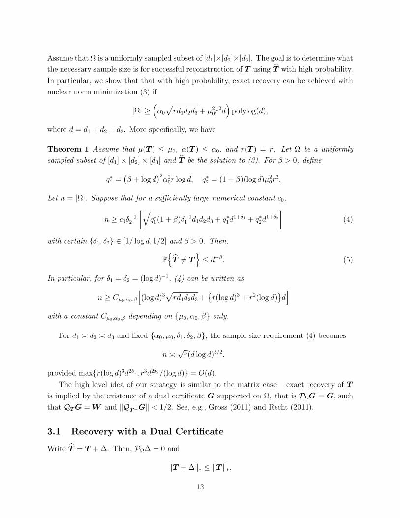
Assume that Ω is a uniformly sampled subset of [d1]×[d2]×[d3]. The goal is to determine what
the necessary sample size is for successful reconstruction of T using T with high probability.
In particular, we show that that with high probability, exact recovery can be achieved with
nuclear norm minimization (3) if
|Ω| ≥(α0
√rd1d2d3 + µ2
0r2d)polylog(d),
where d = d1 + d2 + d3. More specifically, we have
Theorem 1 Assume that µ(T ) ≤ µ0, α(T ) ≤ α0, and r(T ) = r. Let Ω be a uniformly
sampled subset of [d1]× [d2]× [d3] and T be the solution to (3). For β > 0, define
q∗1 =(β + log d
)2α20r log d, q∗2 = (1 + β)(log d)µ2
0r2.
Let n = |Ω|. Suppose that for a sufficiently large numerical constant c0,
n ≥ c0δ−12
[√q∗1(1 + β)δ−1
1 d1d2d3 + q∗1d1+δ1 + q∗2d
1+δ2
](4)
with certain δ1, δ2 ∈ [1/ log d, 1/2] and β > 0. Then,
PT = T
≤ d−β. (5)
In particular, for δ1 = δ2 = (log d)−1, (4) can be written as
n ≥ Cµ0,α0,β
[(log d)3
√rd1d2d3 +
r(log d)3 + r2(log d)
d]
with a constant Cµ0,α0,β depending on µ0, α0, β only.
For d1 ≍ d2 ≍ d3 and fixed α0, µ0, δ1, δ2, β, the sample size requirement (4) becomes
n ≍√r(d log d)3/2,
provided maxr(log d)3d2δ1 , r3d2δ2/(log d) = O(d).
The high level idea of our strategy is similar to the matrix case – exact recovery of T
is implied by the existence of a dual certificate G supported on Ω, that is PΩG = G, such
that QTG = W and ∥QT⊥G∥ < 1/2. See, e.g., Gross (2011) and Recht (2011).
3.1 Recovery with a Dual Certificate
Write T = T +∆. Then, PΩ∆ = 0 and
∥T +∆∥∗ ≤ ∥T ∥∗.
13
Recall that, by Lemma 1, there exists a W obeying W = Q0TW and ∥W ∥ = 1 such that
∥T +∆∥∗ ≥ ∥T ∥∗ + ⟨W +QT⊥W⊥,∆⟩
for any W⊥ obeying ∥W⊥∥ ≤ 1/2. Assume that a tensor G supported on Ω, that is
PΩG = G, such that QTG = W , and ∥QT⊥G∥ < 1/2. When ∥QT⊥∆∥∗ > 0,
⟨W +QT⊥W⊥,∆⟩ = ⟨W +QT⊥W⊥ −G,∆⟩= ⟨W −QTG,∆⟩+ ⟨W⊥,QT⊥∆⟩ − ⟨QT⊥G,QT⊥∆⟩
> ⟨W⊥,QT⊥∆⟩ − 1
2∥QT⊥∆∥∗
Take W⊥ = U/2 where
U = argmaxX:∥X∥≤1
⟨X,QT⊥∆⟩.
We find that ∥QT⊥∆∥∗ > 0 implies
∥T +∆∥∗ − ∥T ∥∗ ≥ ⟨W +QT⊥W⊥,∆⟩ > 0,
which contradicts with fact that T minimizes the nuclear norm. Thus, QT⊥∆ = 0, which
then implies QTQΩQT∆ = QTQΩ∆ = 0. When QTQΩQT is invertible in the range of QT ,
we also have QT∆ = 0 and T = T .
With this in mind, it then suffices to seek such a dual certificate. In fact, it turns out
that finding an “approximate” dual certificate is actually enough for our purposes.
Lemma 4 Assume that
inf∥PΩQTX∥HS : ∥QTX∥HS = 1
≥√
n
2d1d2d3. (6)
If there exists a tensor G supported on Ω such that
∥QTG−W ∥HS <1
4
√n
2d1d2d3and max
∥QT⊥X∥∗=1
⟨G,QT⊥X⟩ ≤ 1/4, (7)
then T = T .
Proof of Lemma 4. Write T = T +∆, then PΩ∆ = 0 and
∥T +∆∥∗ ≤ ∥T ∥∗.
Recall that, by Lemma 1, there exists a W obeying W = Q0TW and ∥W ∥ = 1 such that
for any W⊥ obeying ∥W⊥∥ ≤ 1/2,
∥T +∆∥∗ ≥ ∥T ∥∗ + ⟨W +QT⊥W⊥,∆⟩.
14
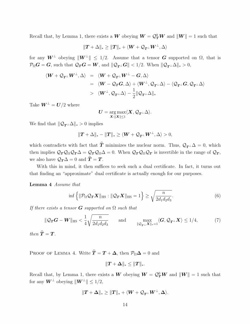
Since ⟨G,∆⟩ = ⟨PΩG,∆⟩ = ⟨G,PΩ∆⟩ = 0 and QTW = W ,
0 ≥ ⟨W +QT⊥W⊥,∆⟩= ⟨W +QT⊥W⊥ −G,∆⟩= ⟨QTW −QTG,∆⟩+ ⟨W⊥,QT⊥∆⟩ − ⟨G,QT⊥∆⟩
≥ −∥W −QTG∥HS∥QT∆∥HS + ⟨W⊥,QT⊥∆⟩ − 1
4∥QT⊥∆∥∗.
In particular, taking W⊥ satisfying ∥W ∥ = 1/2 and ⟨W⊥,QT⊥∆⟩ = ∥QT⊥∆∥∗/2, we find
1
4∥QT⊥∆∥∗ ≤ ∥W −QTG∥HS∥QT∆∥HS.
Recall that PΩ∆ = PΩQT⊥∆+ PΩQT∆ = 0. Thus, in view of the condition on PΩ,
∥QT∆∥HS√2d1d2d3/n
≤ ∥PΩQT∆∥HS = ∥PΩQT⊥∆∥HS ≤ ∥QT⊥∆∥HS ≤ ∥QT⊥∆∥∗. (8)
Consequently,
1
4∥QT⊥∆∥∗ ≤
√2d1d2d3/n∥W −QTG∥HS∥QT⊥∆∥∗.
Since √2d1d2d3/n∥W −QTG∥HS < 1/4,
we have ∥QT⊥∆∥∗ = 0. Together with (8), we conclude that ∆ = 0, or equivalently T = T .
Equation (6) indicates the invertibility of PΩ when restricted to the range of QT . We
argue first that this is true for “incoherent” tensors. To this end, we prove that∥∥∥QT
((d1d2d3/n)PΩ − I
)QT
∥∥∥ ≤ 1/2
with high probability. This implies that as an operator in the range of QT , the spectral
norm of (d1d2d3/n)QTPΩQT is contained in [1/2, 3/2]. Consequently, (6) holds because for
any X ∈ Rd1×d2×d3 ,
(d1d2d3/n)∥PΩQTX∥2HS =⟨QTX, (d1d2d3/n)QTPΩQTX
⟩≥ 1
2∥QTX∥2HS.
Recall that d = d1 + d2 + d3. We have
Lemma 5 Assume µ(T ) ≤ µ0, r(T ) = r, and Ω is uniformly sampled from [d1]× [d2]× [d3]
without replacement. Then, for any τ > 0,
P∥∥QT
((d1d2d3/n)PΩ − I
)QT
∥∥ ≥ τ≤ 2r2d exp
(− τ 2/2
1 + 2τ/3
( n
µ20r
2d
)).
In particular, taking τ = 1/2 in Lemma 5 yields
P(6) holds
≥ 1− 2r2d exp
(− 3
32
( n
µ20r
2d
)).
15
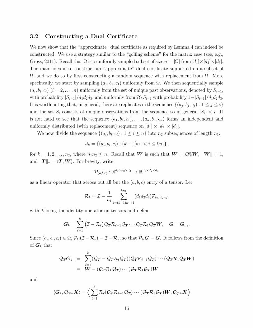
3.2 Constructing a Dual Certificate
We now show that the “approximate” dual certificate as required by Lemma 4 can indeed be
constructed. We use a strategy similar to the “golfing scheme” for the matrix case (see, e.g.,
Gross, 2011). Recall that Ω is a uniformly sampled subset of size n = |Ω| from [d1]×[d2]×[d3].
The main idea is to construct an “approximate” dual certificate supported on a subset of
Ω, and we do so by first constructing a random sequence with replacement from Ω. More
specifically, we start by sampling (a1, b1, c1) uniformly from Ω. We then sequentially sample
(ai, bi, ci) (i = 2, . . . , n) uniformly from the set of unique past observations, denoted by Si−1,
with probability |Si−1|/d1d2d3; and uniformly from Ω\Si−1 with probability 1−|Si−1|/d1d2d3.It is worth noting that, in general, there are replicates in the sequence (aj, bj, cj) : 1 ≤ j ≤ iand the set Si consists of unique observations from the sequence so in general |Si| < i. It
is not hard to see that the sequence (a1, b1, c1), . . . , (an, bn, cn) forms an independent and
uniformly distributed (with replacement) sequence on [d1]× [d2]× [d3].
We now divide the sequence (ai, bi, ci) : 1 ≤ i ≤ n into n2 subsequences of length n1:
Ωk = (ai, bi, ci) : (k − 1)n1 < i ≤ kn1 ,
for k = 1, 2, . . . , n2, where n1n2 ≤ n. Recall that W is such that W = Q0TW , ∥W ∥ = 1,
and ∥T ∥∗ = ⟨T ,W ⟩. For brevity, write
P(a,b,c) : Rd1×d2×d3 → Rd1×d2×d3
as a linear operator that zeroes out all but the (a, b, c) entry of a tensor. Let
Rk = I − 1
n1
kn1∑i=(k−1)n1+1
(d1d2d3)P(ai,bi,ci)
with I being the identity operator on tensors and define
Gk =k∑
ℓ=1
(I −Rℓ
)QTRℓ−1QT · · · QTR1QTW , G = Gn2 .
Since (ai, bi, ci) ∈ Ω, PΩ(I −Rk) = I −Rk, so that PΩG = G. It follows from the definition
of Gk that
QTGk =k∑
ℓ=1
(QT −QTRℓQT )(QTRℓ−1QT ) · · · (QTR1QTW )
= W − (QTRkQT ) · · · (QTR1QT )W
and
⟨Gk,QT⊥X⟩ =⟨ k∑
ℓ=1
Rℓ(QTRℓ−1QT ) · · · (QTR1QT )W ,QT⊥X⟩.
16
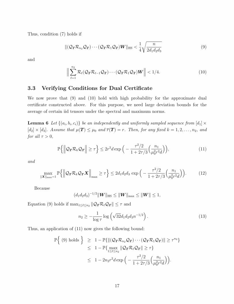
Thus, condition (7) holds if
∥(QTRn2QT ) · · · (QTR1QT )W ∥HS <1
4
√n
2d1d2d3(9)
and ∥∥∥ n2∑ℓ=1
Rℓ(QTRℓ−1QT ) · · · (QTR1QT )W∥∥∥ < 1/4. (10)
3.3 Verifying Conditions for Dual Certificate
We now prove that (9) and (10) hold with high probability for the approximate dual
certificate constructed above. For this purpose, we need large deviation bounds for the
average of certain iid tensors under the spectral and maximum norms.
Lemma 6 Let (ai, bi, ci) be an independently and uniformly sampled sequence from [d1]×[d2]× [d3]. Assume that µ(T ) ≤ µ0 and r(T ) = r. Then, for any fixed k = 1, 2, . . . , n2, and
for all τ > 0,
P∥∥∥QTRkQT
∥∥∥ ≥ τ≤ 2r2d exp
(− τ 2/2
1 + 2τ/3
( n1
µ20r
2d
)), (11)
and
max∥X∥max=1
P∥∥∥QTRkQTX
∥∥∥max
≥ τ≤ 2d1d2d3 exp
(− τ 2/2
1 + 2τ/3
( n1
µ20r
2d
)). (12)
Because
(d1d2d3)−1/2∥W ∥HS ≤ ∥W ∥max ≤ ∥W ∥ ≤ 1,
Equation (9) holds if max1≤ℓ≤n2 ∥QTRℓQT ∥ ≤ τ and
n2 ≥ − 1
log τlog(√
32d1d2d3n−1/2
). (13)
Thus, an application of (11) now gives the following bound:
P(9) holds
≥ 1− P∥(QTRn2QT ) · · · (QTR1QT )∥ ≥ τn2≤ 1− P max
1≤ℓ≤n2
∥QTRℓQT ∥ ≥ τ
≤ 1− 2n2r2d exp
(− τ 2/2
1 + 2τ/3
( n1
µ20r
2d
)).
17

Now consider Equation (10). Let W ℓ = QTRℓQTW ℓ−1 for ℓ ≥ 1 with W 0 = W .
Observe that (10) does not hold with at most probability
P∥∥∥ n2∑
ℓ=1
RℓW ℓ−1
∥∥∥ ≥ 1/4
≤ P∥∥R1W 0
∥∥ ≥ 1/8+ P
∥∥W 1
∥∥max
≥ ∥W ∥max/2
+P∥∥∥ n2∑
ℓ=2
RℓW ℓ−1
∥∥∥ ≥ 1/8,∥∥W 1
∥∥max
< ∥W ∥max/2
≤ P∥∥R1W 0
∥∥ ≥ 1/8+ P
∥∥W 1
∥∥max
≥ ∥W ∥max/2
+P∥∥R2W 1
∥∥ ≥ 1/16,∥∥W 1
∥∥max
< ∥W ∥max/2
+P∥∥W 2
∥∥max
≥ ∥W ∥max/4,∥∥W 1
∥∥max
< ∥W ∥max/2
+P∥∥∥ n2∑
ℓ=3
RℓW ℓ−1
∥∥∥ ≥ 1
16,∥∥W 2
∥∥max
< ∥W ∥max/4
≤n2−1∑ℓ=1
P∥∥QTRℓQTW ℓ−1
∥∥max
≥ ∥W ∥max/2ℓ,∥∥W ℓ−1
∥∥max
≤ ∥W ∥max/2ℓ−1
+
n2∑ℓ=1
P∥∥RℓW ℓ−1
∥∥ ≥ 2−2−ℓ,∥∥W ℓ−1
∥∥max
≤ ∥W ∥max/2ℓ−1.
Since Rℓ,W ℓ are i.i.d., (12) with X = W ℓ−1/∥W ℓ−1∥max implies
P(10) holds
≥ 1− n2 max
X:X=QTX∥X∥max≤1
(P∥∥∥QTR1QTX
∥∥∥max
>1
2
+ P
∥∥∥R1X∥∥∥ >
1
8∥W ∥max
)
≥ 1− 2n2d1d2d3 exp(−(3/32)n1
µ20r
2d
)− n2 max
X:X=QTX∥X∥max≤∥W ∥max
P∥∥∥R1X
∥∥∥ >1
8
.
The last term on the right hand side can be bounded using the following result.
Lemma 7 Assume that α(T ) ≤ α0, r(T ) = r and q∗1 =(β + log d
)2α20r log d. There exists
a numerical constant c1 > 0 such that for any constants β > 0 and 1/(log d) ≤ δ1 < 1,
n1 ≥ c1
[q∗1d
1+δ1 +√q∗1(1 + β)δ−1
1 d1d2d3
](14)
implies
maxX:X=QTX
∥X∥max≤∥W ∥max
P∥∥∥R1X
∥∥∥ ≥ 1
8
≤ d−β−1, (15)
18

where W is in the range of Q0T such that ∥W ∥ = 1 and ⟨T ,W ⟩ = ∥T ∥∗.
3.4 Proof of Theorem 1
Since (7) is a consequence of (9) and (10), it follows from Lemmas 4, 5, 6 and 7 that for
τ ∈ (0, 1/2] and n ≥ n1n2 satisfying conditions (13) and (14),
PT = T
≤ 2r2d exp
(− 3
32
( n
µ20r
2d
))+ 2n2r
2d exp(− τ 2/2
1 + 2τ/3
( n1
µ20r
2d
))+2n2d1d2d3 exp
(−(3/32)n1
µ20r
2d
)+ n2d
−β−1.
We now prove Theorem 1 by setting τ = d−δ2/2/2, so that condition (13) can be written as
n2 ≥ c2/δ2. Assume without loss of generality n2 ≤ d/2 because large c0 forces large d. For
sufficiently large c′2, the right-hand side of the above inequality is no greater than d−β when
n1 ≥ c′2(1 + β)(log d)µ20r
2d/(4τ 2) = c′2q∗2d
1+δ2
holds as well as (14). Thus, (4) implies (5) for sufficiently large c0.
4 Concentration Inequalities for Low Rank Tensors
We now prove Lemmas 5 and 6, both involving tensors of low rank. We note that Lemma 5
concerns the concentration inequality for the sum of a sequence of dependent tensors whereas
in Lemma 6, we are interested in a sequence of iid tensors.
4.1 Proof of Lemma 5
We first consider Lemma 5. Let (ak, bk, ck) be sequentially uniformly sampled from Ω∗
without replacement, Sk = (aj, bj, cj) : j ≤ k, and mk = d1d2d3 − k. Given Sk, the
conditional expectation of P(ak+1,bk+1,ck+1) is
E[P(ak+1,bk+1,ck+1)
∣∣∣Sk
]=
PSck
mk
.
For k = 1, . . . , n, define martingale differences
Dk = d1d2d3(mn/mk)QT
(P(ak,bk,ck) − PSc
k−1/mk−1
)QT .
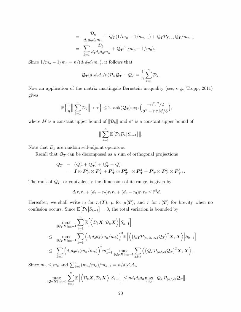
Because PSc0= I and Sn = Ω, we have
QTPΩQT /mn =Dn
d1d2d3mn
+QT (PScn−1
/mn−1)QT /mn +QTPSn−1QT /mn
19
=Dn
d1d2d3mn
+QT (1/mn − 1/mn−1) +QTPSn−1QT /mn−1
=n∑
k=1
Dk
d1d2d3mn
+QT (1/mn − 1/m0).
Since 1/mn − 1/m0 = n/(d1d2d3mn), it follows that
QT (d1d2d3/n)PΩQT −QT =1
n
n∑k=1
Dk.
Now an application of the matrix martingale Bernstein inequality (see, e.g., Tropp, 2011)
gives
P 1n
∥∥∥ n∑k=1
Dk
∥∥∥ > τ≤ 2 rank(QT ) exp
( −n2τ 2/2
σ2 + nτM/3
),
where M is a constant upper bound of ∥Dk∥ and σ2 is a constant upper bound of∥∥ n∑k=1
E[DkDk|Sk−1
]∥∥.Note that Dk are random self-adjoint operators.
Recall that QT can be decomposed as a sum of orthogonal projections
QT = (Q0T +Q1
T ) +Q2T +Q3
T
= I ⊗ P 2T ⊗ P 3
T + P 1T ⊗ P 2
T⊥ ⊗ P 3T + P 1
T ⊗ P 2T ⊗ P 3
T⊥ .
The rank of QT , or equivalently the dimension of its range, is given by
d1r2r3 + (d2 − r2)r1r3 + (d3 − r3)r1r2 ≤ r2d.
Hereafter, we shall write rj for rj(T ), µ for µ(T ), and r for r(T ) for brevity when no
confusion occurs. Since E[Dk
∣∣Sk−1
]= 0, the total variation is bounded by
max∥QTX∥HS=1
n∑k=1
E[⟨
DkX,DkX⟩∣∣∣Sk−1
]≤ max
∥QTX∥HS=1
n∑k=1
(d1d2d3(mn/mk)
)2E[⟨(
QTP(ak,bk,ck)QT
)2X,X
⟩∣∣∣Sk−1
]≤
n∑k=1
(d1d2d3(mn/mk)
)2m−1
k−1 max∥QTX∥HS=1
∑a,b,c
⟨(QTP(a,b,c)QT
)2X,X
⟩.
Since mn ≤ mk and∑n
k=1(mn/mk)/mk−1 = n/d1d2d3,
max∥QTX∥HS=1
n∑k=1
E[⟨
DkX,DkX⟩∣∣∣Sk−1
]≤ nd1d2d3max
a,b,c
∥∥QTP(a,b,c)QT
∥∥.20

It then follows that
maxa,b,c
∥∥QTP(a,b,c)QT
∥∥ = max∥QTX∥HS=1
⟨QTP(a,b,c)QTX,QTX
⟩= max
∥QTX∥HS=1
⟨QTea ⊗ eb ⊗ ec,QTX
⟩2≤ µ2r2d
d1d2d3.
Consequently, we may take σ2 = nµ20r
2d. Similarly,
M ≤ maxk
d1d2d3(mn/mk)2maxa,b,c
∥∥QTP(a,b,c)QT
∥∥ ≤ 2µ2r2d.
Inserting the expression and bounds for rank(QT ), σ2 and M into the Bernstein inequality,
we find
P 1n
∥∥∥ n∑k=1
Dk
∥∥∥ > τ≤ 2(r2d) exp
( −τ 2/2
1 + 2τ/3
( n
µ2r2d
)),
which completes the proof because µ(T ) ≤ µ0 and r(T ) = r.
4.2 Proof of Lemma 6.
In proving Lemma 6, we consider first (12). Let X be a tensor with ∥X∥max ≤ 1. Similar
to before, write
Di = d1d2d3QTP(ai,bi,ci) −QT
for i = 1, . . . , n1. Again, we shall also write µ for µ(T ), and r for r(T ) for brevity. Observe
that for each point (a, b, c) ∈ [d1]× [d2]× [d3],
1
d1d2d3
∣∣⟨ea ⊗ eb ⊗ ec,DiX⟩∣∣
=∣∣∣⟨QT (ea ⊗ eb ⊗ ec),QT (eak ⊗ ebk ⊗ eck)⟩X(ak, bk, ck)− ⟨QT (ea ⊗ eb ⊗ ec),QTX⟩/(d1d2d3)
∣∣∣≤ 2max
a,b,c∥QT (ea ⊗ eb ⊗ ec)∥2HS∥X∥max
≤ 2µ2r2d/(d1d2d3).
Since the variance of a variable is no greater than the second moment,
E(
1
d1d2d3
∣∣⟨ea ⊗ eb ⊗ ec,QTDiX⟩∣∣)2
≤ E∣∣⟨QT (ea ⊗ eb ⊗ ec),QT (ea′ ⊗ eb′ ⊗ ec′)⟩X(ak, bk, ck)
∣∣2≤ 1
d1d2d3
∑a′,b′,c′
∣∣⟨QTea ⊗ eb ⊗ ec,QT (ea′ ⊗ eb′ ⊗ ec′)⟩∣∣2
=1
d1d2d3∥QT (ea ⊗ eb ⊗ ec)∥2HS
21
≤ µ2r2d/(d1d2d3)2.
Since ⟨ea ⊗ eb ⊗ ec,QTDiX⟩ are iid random variables, the Bernstein inequality yields
P∣∣∣ 1
n1
n1∑i=1
⟨ea ⊗ eb ⊗ ec,QTDiX⟩∣∣∣ > τ
≤ 2 exp
(− (n1τ)
2/2
n1µ2r2d+ n1τ2µ2r2d/3
).
This yields (12) by the union bound.
The proof of (11) is similar, but the matrix Bernstein inequality is used. We equip
Rd1×d2×d3 with the Hilbert-Schmidt norm so that it can be viewed as the Euclidean space.
As linear maps in this Euclidean space, the operators Di are just random matrices. Since
the projection P(a,b,c) : X → ⟨ea ⊗ eb ⊗ ec,X⟩ea ⊗ eb ⊗ ec is of rank 1,
∥QTP(a,b,c)QT ∥ = ∥QT (ea ⊗ eb ⊗ ec)∥2HS ≤ µ2r2d/(d1d2d3).
It follows that ∥Di∥ ≤ 2µ2r2d. Moreover, Di is a self-adjoint operator and its covariance
operator is bounded by
max∥X∥HS=1
E∥∥DiX∥2HS ≤ (d1d2d3)
2 max∥X∥HS=1
E⟨(
QTP(ak,bk,ck)QT
)2X,X
⟩≤ d1d2d3
∑a,b,c
∥QT (ea ⊗ eb ⊗ ec)∥2HS
⟨ea ⊗ eb ⊗ ec,X
⟩2≤ d1d2d3 max
a,b,c∥QT (ea ⊗ eb ⊗ ec)∥2HS
= µ2r2d
Consequently, by the matrix Bernstein inequality (Tropp, 2011),
P∥∥∥ 1
n1
n1∑i=1
Di
∥∥∥ > τ≤ 2 rank(QT ) exp
( τ 2/2
1 + 2τ/3
( n1
µ2r2d
)).
This completes the proof due to the fact that rank(QT ) ≤ r2d.
5 Concentration Inequalities for Sparse Tensors
We now derive probabilistic bounds for ∥RℓX∥ when (ai, bi, ci)s are iid vectors uniformly
sampled from [d1]× [d2]× [d3] and X = QTX with small ∥X∥max.
5.1 Symmetrization
We are interested in bounding
maxX∈U (η)
P
∥∥∥∥∥d1d2d3n
n∑i=1
P(ai,bi,ci)X −X
∥∥∥∥∥ ≥ t
,
22
e.g. with (n, η, t) replaced by (n1, (α0
√r) ∧
√d1d2d3, 1/8) in the proof of Lemma 7, where
U (η) = X : QTX = X, ∥X∥max ≤ η/√d1d2d3.
Our first step is symmetrization.
Lemma 8 Let ϵis be a Rademacher sequence, that is a sequence of i.i.d. ϵi with Pϵi = 1 =
Pϵi = −1 = 1/2. Then
maxX∈U (η)
P
∥∥∥∥∥d1d2d3n
n∑i=1
P(ai,bi,ci)X −X
∥∥∥∥∥ ≥ t
≤ 4 maxX∈U (η)
P
∥∥∥∥∥d1d2d3n
n∑i=1
ϵiP(ai,bi,ci)X
∥∥∥∥∥ ≥ t/2
+ 4 exp
(− nt2/2
η2 + 2ηt√d1d2d3/3
).
Proof of Lemma 8. Following a now standard Gine-Zinn type of symmetrization
argument, we get
maxX∈U (η)
P
∥∥∥∥∥d1d2d3n
n∑i=1
P(ai,bi,ci)X −X
∥∥∥∥∥ ≥ t
≤ 4 maxX∈U (η)
P
∥∥∥∥∥d1d2d3n
n∑i=1
ϵiP(ai,bi,ci)X
∥∥∥∥∥ ≥ t/2
+2 maxX∈U (η)
max∥u∥=∥v∥=∥w∥=1
P⟨
u⊗ v ⊗w,d1d2d3
n
n∑i=1
P(ai,bi,ci)X −X⟩> t.
See, e.g., Gine and Zinn (1984). It remains to bound the second quantity on the right-hand
side. To this end, denote by
ξi =⟨u⊗ v ⊗w, d1d2d3P(ai,bi,ci)X −X
⟩.
For ∥u∥ = ∥v∥ = ∥w∥ = 1 and X ∈ U (η), ξi are iid variables with Eξi = 0, |ξi| ≤2d1d2d3∥X∥max ≤ 2η
√d1d2d3 and Eξ2i ≤ (d1d2d3)∥X∥2max ≤ η2. Thus, the statement follows
from the Bernstein inequality. In the light of Lemma 8, it suffices to consider bounding
maxX∈U (η)
P
∥∥∥∥∥d1d2d3n
n∑i=1
ϵiP(ai,bi,ci)X
∥∥∥∥∥ ≥ t/2
.
To this end, we use a thinning method to control the spectral norm of tensors.
23
5.2 Thinning of the spectral norm of tensors
Recall that the spectral norm of a tensor Z ∈ Rd1×d2×d3 is defined as
∥Z∥ = maxu∈Rd1 ,v∈Rd2 ,w∈Rd3
∥u∥∨∥v∥∨∥w∥≤1
⟨u⊗ v ⊗w,Z⟩.
We first use a thinning method to discretize maximization in the unit ball in Rdj to the
problem involving only vectors taking values 0 or ±2−ℓ/2, ℓ ≤ mj := ⌈log2 dj⌉, that is, binary“digitalized” vectors that belong to
Bmj ,dj = 0,±1,±2−1/2, . . . ,±2−mj/2d ∩ u ∈ Rdj : ∥u∥ ≤ 1. (16)
Lemma 9 For any tensor Z ∈ Rd1×d2×d3,
∥Z∥ ≤ 8max⟨u⊗ v ⊗w,Z⟩ : u ∈ Bm1,d1 ,v ∈ Bm2,d2 ,w ∈ Bm3,d3
,
where mj := ⌈log2 dj⌉, j = 1, 2, 3.
Proof of Lemma 9. Denote by
Cm,d = min∥a∥=1
maxu∈Bm,d
u⊤a,
which bounds the effect of discretization. Let X be a linear mapping from Rd to a linear
space equipped with a seminorm ∥ · ∥. Then, ∥Xu∥ can be written as the maximum of
ϕ(Xu) over linear functionals ϕ(·) of unit dual norm. Since max∥u∥≤1 u⊤a = 1 for ∥a∥ = 1,
it follows from the definition of Cm,d that
max∥u∥≤1
u⊤a ≤ ∥a∥C−1m,d max
u∈Bm,d
u⊤(a/∥a∥) = C−1m,d max
u∈Bm,d
u⊤a
for every a ∈ Rd with ∥a∥ > 0. Consequently, for any positive integer m,
max∥u∥≤1
∥Xu∥ = maxa:a⊤v=ϕ(Xv)∀v
max∥u∥≤1
a⊤u ≤ C−1m,d max
u∈Bm,d
∥Xu∥.
An application of the above inequality to each coordinate yields
∥Z∥ ≤ C−1m1,d1
C−1m2,d2
C−1m3,d3
maxu∈Bm1,d1
,v∈Bm2,d2,w∈Bm3,d3
⟨u⊗ v ⊗w,Z⟩.
It remains to show that Cmj ,dj ≥ 1/2. To this end, we prove a stronger result that for
any m and d,
C−1m,d ≤
√2 + 2(d− 1)/(2m − 1).
24
Consider first a continuous version of Cm,d:
C ′m,d = min
∥a∥=1max
u∈B′m,d
a⊤u.
where B′m,d = t : t2 ∈ [0, 1] \ (0, 2−m)d ∩ u : ∥u∥ ≤ 1. Without loss of generality, we
confine the calculation to nonnegative ordered a = (a1, . . . , ad)⊤ satisfying 0 ≤ a1 ≤ . . . ≤ ad
and ∥a∥ = 1. Let
k = maxj : 2ma2j +
j−1∑i=1
a2i ≤ 1
and v =(aiIi > k)d×1
1−∑k
i=1 a2i 1/2
.
Because 2mv2k+1 = 2ma2k+1/(1 −∑k
i=1 a2i ) ≥ 1, we have v ∈ B′
m,d. By the definition of k,
there exists x2 ≥ a2k satisfying
(2m − 1)x2 +k∑
i=1
a2i = 1.
It follows that
k∑i=1
a2i =
∑ki=1 a
2i
(2m − 1)x2 +∑k
i=1 a2i
≤ kx2
(2m − 1)x2 + kx2≤ d− 1
2m + d− 2.
Because a⊤v = (1−∑k
i=1 a2i )
1/2 for this specific v ∈ B′m,d, we get
C ′m,d ≥ min
∥a∥2=1
(1−
k∑i=1
a2i
)1/2≥(1− d− 1
2m + d− 2
)1/2=( 2m − 1
2m + d− 2
)1/2.
Now because every v ∈ B′m,d with nonnegative components matches a u ∈ Bm,d with
sgn(vi)√2ui ≥ |vi| ≥ sgn(vi)ui,
we find Cm,d ≥ C ′m,d/
√2. Consequently,
1/Cm,d ≤√2/C ′
m,d ≤√21 + (d− 1)/(2m − 1)1/2.
It follows from Lemma 9 that the spectrum norm ∥Z∥ is of the same order as the
maximum of ⟨u⊗ v ⊗w,Z⟩ over u ∈ Bm1,d1 , v ∈ Bm2,d2 and w ∈ Bm3,d3 . We will further
decompose such tensors u⊗v⊗w according to the absolute value of their entries and bound
the entropy of the components in this decomposition.
25
5.3 Spectral norm of tensors with sparse support
Denote by Dj a “digitalization” operator such that Dj(X) will zero out all entries of X
whose absolute value is not 2−j/2, that is
Dj(X) =∑a,b,c
I|⟨ea ⊗ eb ⊗ ec,X⟩| = 2−j/2
⟨ea ⊗ eb ⊗ ec,X⟩ea ⊗ eb ⊗ ec. (17)
With this notation, it is clear that for u ∈ Bm1,d1 , v ∈ Bm2,d2 and w ∈ Bm3,d3 ,
⟨u⊗ v ⊗w,X⟩ =m1+m2+m3∑
j=0
⟨Dj(u⊗ v ⊗w),X⟩.
The possible choice of Dj(u⊗ v ⊗w) in the above expression may be further reduced if
X is sparse. More specifically, denote by
supp(X) = ω ∈ [d1]× [d2]× [d3] : X(ω) = 0.
Define the maximum aspect ratio of supp(X) as
νsupp(X) = maxℓ=1,2,3
maxik:k =ℓ
|iℓ : (i1, i2, i3) ∈ supp(X)| . (18)
In other words, the quantity νsupp(X) is the maximum ℓ0 norm of the fibers of the third-order
tensor. We observe first that, if supp(X) is a uniformly sampled subset of [d1]× [d2]× [d3],
then it necessarily has a small aspect ratio.
Lemma 10 Let Ω be a uniformly sampled subset of [d1] × [d2] × [d3] without replacement.
Let d = d1 + d2 + d3, p∗ = max(d1, d2, d3)/(d1d2d3), and ν1 = (dδ1enp∗) ∨ (3 + β)/δ1 with
a certain δ1 ∈ [1/ log d, 1]. Then,
PνΩ ≥ ν1
≤ d−β−1/3.
Proof of Lemma 10. Let p1 = d1/(d1d2d3), t = log(ν1/(np∗)) ≥ 1, and
Ni2i3 = |iℓ : (i1, i2, i3) ∈ Ω| .
Because Ni2i3 follows the Hypergeometric(d1d2d3, d1, n) distribution, its moment generating
function is no greater than that of Binomial(n, p1). Due to p1 ≤ p∗,
PNi2i3 ≥ ν1 ≤ exp(−tν1 + np∗(et − 1)
)≤ exp (−ν1 log(ν1/(enp
∗))) .
26
The condition on ν1 implies ν1 log(ν1/(enp∗)) ≥ (3 + β) log d. By the union bound,
Pmaxi2,i3
Ni2i3 ≥ ν1 ≤ d2d3d−3−β.
By symmetry, the same tail probability bound also holds for maxi1,i3 |i2 : (i1, i2, i3) ∈ Ω|and maxi1,i2 |i3 : (i1, i2, i3) ∈ Ω|, so that PνΩ ≥ ν1 ≤ (d1d2 + d1d3 + d2d3)d
−3−β. The
conclusion follows from d1d2 + d1d3 + d2d3 ≤ d2/3.
We are now in position to further reduce the set of maximization in defining the spectrum
norm of sparse tensors. To this end, denote for a block A×B × C ⊆ [d1]× [d2]× [d3],
h(A×B × C) = minν : |A| ≤ ν|B||C|, |B| ≤ ν|A||C|, |C| ≤ ν|A||B|
. (19)
It is clear that for any block A× B × C, there exists A ⊆ A, B ⊆ B and C ⊆ C such that
h(A× B × C) ≤ νΩ and
(A×B × C) ∩ Ω = (A× B × C) ∩ Ω.
For u ∈ Bm1,d1 , v ∈ Bm2,d2 and w ∈ Bm3,d3 , let Ai1 = a : u2a = 2−i1, Bi2 = b : v2b = 2−i2
and Ci3 = c : w2c = 2−i3, and define
Dj(u⊗ v ⊗w) =∑
(i1,i2,i3):i1+i2+i3=j
PAj,i1×Bj,i2
×Cj,i3Dj(u⊗ v ⊗w) (20)
where Aj,i1 ⊆ Aj,i1 , Bj,i2 ⊆ Bj,i2 and Cj,i3 ⊆ Cj,i3 satisfying h(Aj,i1 × Bj,i2 × Cj,i3) ≤ νΩ and
(Ai1 ×Bi2 × Ci3) ∩ Ω = (Aj,i1 × Bj,i2 × Cj,i3) ∩ Ω.
Because PΩDj(u⊗ v ⊗w) is supported in ∪(i1,i2,i3):i1+i2+i3=j(Ai1 ×Bi2 × Ci3) ∩ Ω, we have
PΩDj(u⊗ v ⊗w) = PΩDj(u⊗ v ⊗w).
This observation, together with Lemma 9, leads to the following characterization of the
spectral norm of a tensor support on a set with bounded aspect ratio.
Lemma 11 Let mℓ = ⌈log2 dℓ⌉ for ℓ = 1, 2, 3, and Dj(·) and Dj(·) be as in (17) and (20)
respectively. Define
B∗Ω,m∗ =
∑0≤j≤m∗
Dj(u1 ⊗ u2 ⊗ u3) +∑
m∗<j≤m∗
Dj(u1 ⊗ u2 ⊗ u3) : uℓ ∈ Bmℓ,dℓ
,
and B∗ν,m∗ = ∪νΩ≤νB∗
Ω,m∗. Let X ∈ Rd1×d2×d3 be a tensor with supp(X) ⊆ Ω. For any
0 ≤ m∗ ≤ m1 +m2 +m3 and ν ≥ νΩ,
∥X∥ ≤ 8 maxY ∈B∗
Ω,m∗
⟨Y ,X⟩ ≤ 8 maxY ∈B∗
ν,m∗
⟨Y ,X⟩.
27
5.4 Entropy bounds
Essential to our argument are entropic bounds related to B∗ν,m∗ . It is clear that
#Dj(u) : ∥u∥ ≤ 1 ≤(
dj2k ∧ dj
)22
k∧dj ≤ exp((2k ∧ dj)(log 2 + 1 + (log(dj/2k))+)),
so that by (16)
|Bmj ,dj | ≤mj∏k=0
(dj
2k ∧ dj
)22
k∧dj ≤ exp(dj
∞∑ℓ=1
2−ℓ(log 2 + 1 + log(2ℓ)))≤ exp(4.78 dj)
Consequently, due to d = d1 + d2 + d3 and 4.78 ≤ 21/4,
∣∣B∗ν,m∗
∣∣ ≤ 3∏j=1
|Bmj ,dj | ≤ e(21/4)d. (21)
We derive tighter entropy bounds for slices of B∗ν,m∗ by considering
Dν,j,k =Dj(Y ) : Y ∈ B∗
ν,m∗ , ∥Dj(Y )∥2HS ≤ 2k−j.
Here and in the sequel, we suppress the dependence of D on quantities such asm∗,m1,m2,m3
for brevity, when no confusion occurs.
Lemma 12 Let L(x, y) = max1, log(ey/x) and ν ≥ 1. For all 0 ≤ k ≤ j ≤ m∗,
log∣∣∣Dν,j,k
∣∣∣ ≤ (21/4)J(ν, j, k), (22)
where J(ν, j, k) = (j + 2)√ν2k−1L
(√ν2k−1, (j + 2)d
).
Proof of Lemma 12. We first bound the entropy of a single block. Let
D (block)ν,ℓ =
sgn(ua)sgn(vb)sgn(wc)I(a, b, c) ∈ A×B × C :
h(A×B × C) ≤ ν, |A||B||C| = ℓ.
By the constraints on the size and aspect ratio of the block,
max(|A|2, |B|2, |C|2) ≤ ν|A||B||C| ≤ νℓ.
By dividing D (block)ν,ℓ into subsets according to (ℓ1, ℓ2, ℓ3) = (|A|, |B|, |C|), we find∣∣∣D (block)
ν,ℓ
∣∣∣ ≤ ∑ℓ1ℓ2ℓ3=ℓ,max(ℓ1,ℓ2,ℓ3)≤
√νℓ
2ℓ1+ℓ2+ℓ3
(d1ℓ1
)(d2ℓ2
)(d3ℓ3
)
28

By the Stirling formula, for i = 1, 2, 3,
log[√
2πℓi2ℓi
(diℓi
)]≤ ℓiL
(ℓi, 2d
)≤
√νℓ L
(√νℓ, 2d
).
We note that k(k + 1)/(2√
qk) is no greater than 2.66, 1.16 and 1 respectively for q = 2,
q = 3 and q ≥ 5. Let ℓ =∏m
j=1 qkjj with distinct prime factors qj. We get
|(ℓ1, ℓ2, ℓ3) : ℓ1ℓ2ℓ3 = ℓ| =m∏j=1
(kj + 1
2
)≤ 2.66× 1.16
m∏j=1
√qkjj ≤ πℓ1/2 ≤
3∏i=1
√2πℓi.
It follows that ∣∣∣D (block)ν,ℓ
∣∣∣ ≤ exp(3√νℓL
(√νℓ, 2d
)). (23)
Due to the constraint i1 + i2 + i3 = j in defining B∗ν,m∗ , for any Y ∈ B∗
ν,m∗ , Dj(Y ) is
composed of at most i∗ =(j+22
)blocks. Since the sum of the sizes of the blocks is bounded
by 2k, (23) yields
∣∣∣Dν,j,k
∣∣∣ ≤∑
ℓ1+...+ℓi∗≤2k
i∗∏i=1
∣∣∣D (block)νℓi
∣∣∣≤
∑ℓ1+...+ℓi∗≤2k
exp( i∗∑
i=1
3√νℓi L
(√νℓi, 2d
))≤ (2k)i
∗max
ℓ1+...+ℓi∗≤2kexp
( i∗∑i=1
3√
νℓi L(√
νℓi, 2d))
.
It follows from the definition of L(x, y) and the Cauchy-Schwarz inequality that
i∗∑i=1
√ℓi L
(√νℓi, 2d
)=
i∗∑i=1
√ℓi
(L(√
ν2k, 2d)+ log
(√2k/ℓi
))≤
√2k(√
i∗L(√
ν2k, 2d)+
i∗∑i=1
√ℓi/2k log
(√2k/ℓi
))≤
√i∗2k
(L(√
ν2k, 2d)+ log
(√i∗))
,
where the last inequality above follows from the fact that subject to u1, u2 ≥ 0 and u21+u2
2 ≤2c2 ≤ 2, the maximum of −u1 log(u1)− u2 log(u2) is attained at u1 = u2 = c. Consequently,
since i∗ ≤(j+22
),
log∣∣∣Dν,j,k
∣∣∣ ≤ i∗ log(2k)+ 3
√i∗ν2kL
(√ν2k, 2d
√(j+22
)).
29
We note that j ≥ k,√2k ≥ k
√8/3, ν ≥ 1 and xL(x, y) is increasing in x, so that
√i∗ν2kL
(√ν2k, 2d
√(j+22
))i∗ log
(2k) ≥
√8/3L
(k√8/2, 2d
√(j+22
))√i∗ log 2
≥√8 log(ed)√i∗ log 8
.
Moreover, because 2m∗+3/2 ≤
√8∏3
j=1(2dj) ≤√8(2d/3)3 ≤ d3, we get
√2i∗ ≤√
(j + 1)(j + 2) ≤ j + 3/2 ≤ m∗ + 3/2 ≤ (3/ log 2) log d, so that the right-hand side of
the above inequality is no smaller than (4/ log 8)(log 2)/3 = 4/9. It follows that
log∣∣∣Dν,j,k
∣∣∣ ≤ (3 + 9/4)√i∗ν2kL
(√ν2k, 2d
√(j+22
)).
This yields (22) due to i∗ ≤(j+22
).
By (21), the entropy bound in Lemma 12 is useful only when 0 ≤ k ≤ j ≤ m∗, where
m∗ = minx : x ≥ m∗ or J(ν1, x, x) ≥ d
. (24)
5.5 Probability bounds
We are now ready to derive a useful upper bound for
maxX∈U (η)
P
∥∥∥∥∥d1d2d3n
n∑i=1
ϵiP(ai,bi,ci)X
∥∥∥∥∥ ≥ t
.
Let X ∈ U (η). For brevity, write Zi = d1d2d3ϵiP(ai,bi,ci)X and
Z =d1d2d3
n
n∑i=1
ϵiP(ai,bi,ci)X =1
n
n∑i=1
Zi.
Let Ω = (ai, bi, ci) : i ≤ n. In the light of Lemma 10, we shall proceed conditional on the
event that νΩ ≤ ν1 in this subsection. In this event, Lemma 11 yields
∥Z∥ ≤ 8 maxY ∈B∗
ν1,m∗
⟨Y ,Z⟩ (25)
= 8 maxY ∈B∗
ν1,m∗
( ∑0≤j≤m∗
⟨Dj(Y ),Z⟩+ ⟨S∗(Y ),Z⟩
),
where m∗ is as in (24) with the given ν1 and S∗(Y ) =∑
j>m∗Dj(Y ).
Let Y ∈ B∗ν1,m∗ and Y j = Dj(Y ). Recall that for Y j = 0, 2−j ≤ ∥Y j∥2HS ≤ 1, so that
Y j ∈ ∪jk=0Dν1,j,k. To bound the first term on the right-hand side of (25), consider
P
maxY j∈Dν1,j,k
\Dν1,j,k−1
⟨Y j,Z⟩ ≥ t(m∗ + 2)−1/2∥Y j∥HS
30

with 0 ≤ k ≤ j ≤ m∗. Because ∥Zi∥max ≤ d1d2d3∥X∥max ≤ η√d1d2d3, for any Y j ∈ Dν1,j,k,
|⟨Y j,Zi⟩| ≤ 2−j/2η√
d1d2d3, E⟨Y j,Zi⟩2 ≤ η2∥Y j∥2HS ≤ η22k−j.
Let h0(u) = (1 + u) log(1 + u)− u. By Bennet’s inequality,
P⟨Y j,Z⟩ ≥ t2(k−j−1)/2(m∗ + 2)−1/2
≤ exp
(− n(η22k−j)
2−jη2d1d2d3h0
((t2(k−j−1)/2(m∗ + 2)−1/2)(2−j/2η
√d1d2d3)
η22k−j
))= exp
(− n2k
d1d2d3h0
(t√d1d2d3
η√(m∗ + 2)2k+1
)).
Recall that Dν,j,k =Y j = Dj(Y ) : Y ∈ B∗
ν,m∗ , ∥Y j∥2HS ≤ 2k−j. By Lemma 12,
P
maxY j∈Dν1,j,k
\Dν1,j,k−1
⟨Y j,Z⟩ ≥ t(m∗ + 2)−1/2∥Y j∥HS
≤ |Dν1,j,k| max
Y j∈Dν1,j,k
P⟨Y j,Z⟩ ≥ t2(k−j−1)/2(m∗ + 2)−1/2
(26)
≤ exp
((21/4)J(ν1, j, k)−
n2k
d1d2d3h0
(t√d1d2d3
η√(m∗ + 2)2k+1
)).
Let Lk = 1 ∨ log(ed(m∗ + 2)/√ν12k−1). By the definition of J(ν, j, k) in Lemma 12,
J(ν1, j, k) ≤ J(ν1,m∗, k) = (m∗ + 2)√2k−1ν1Lk ≤ J(ν1,m∗,m∗) = d.
Let x ≥ 1 and t1 be a constant satisfying
nt1 ≥ 24η(m∗ + 2)3/2√
ν1d1d2d3, nxt21h0(1) ≥ 12η2(m∗ + 2)2√edL0. (27)
We prove that for all x ≥ 1 and 0 ≤ k ≤ j ≤ m∗
n2k
d1d2d3h0
(xt1
√d1d2d3
η√
(m∗ + 2)2k+1
)≥ 6xJ(ν1,m∗, k) ≥ 6xJ(ν1, j, k). (28)
Consider the following three cases:
Case 1:xt1
√d1d2d3
η√(m∗ + 2)2k+1
≥[max
1,
ed(m∗ + 2)√ν12k−1
]1/2,
Case 2: 1 <xt1
√d1d2d3
η√(m∗ + 2)2k+1
≤[ed(m∗ + 2)√
ν12k−1
]1/2,
Case 3:xt1
√d1d2d3
η√(m∗ + 2)2k+1
≤ 1.
31
Case 1: Due to h0(u) ≥ (u/2) log(1 + u) for u ≥ 1 and the lower bound for nt1,
n2k
d1d2d3h0
(xt1
√d1d2d3
η√
(m∗ + 2)2k+1
)≥ n2k
d1d2d3
(xt1
√d1d2d3
η√
(m∗ + 2)2k+1
)Lk
4
≥ 6x(m∗ + 2)√
ν12k−1Lk.
Case 2: Due to (m∗ + 2)√2k−1ν1 ≤ d, we have
1√d1d2d3
≥ xt1√e(m∗ + 2)
η√
(m∗ + 2)2k+1
[ed(m∗ + 2)√
ν12k−1
]−1
=xt1
√ν12k−1
ηd√e(m∗ + 2)2k+1
.
Thus, due to h0(u) ≥ uh0(1) for u ≥ 1, we have
n2k
d1d2d3h0
(xt1
√d1d2d3
η√
(m∗ + 2)2k+1
)≥
( xt1√ν12k−1
ηd√e(m∗ + 2)2k+1
)n√2k−1xt1h0(1)
η√m∗ + 2
=nx2t21h0(1)
√ν12k−1
2η2(m∗ + 2)√ed
.
Because nxt21h0(1) ≥ 12η2(m∗ + 2)2√edL0 and L0 ≥ Lk, it follows that
n2k
d1d2d3h0
(xt1
√d1d2d3
η√
(m∗ + 2)2k+1
)≥ 6x(m∗ + 2)
√ν12k−1Lk.
Case 3: Due to h0(u) ≥ u2h0(1) for 0 ≤ u ≤ 1 and nxt21h0(1) ≥ 12η2(m∗ + 2)d, we have
n2k
d1d2d3h0
(xt1
√d1d2d3
η√(m∗ + 2)2k+1
)≥ nx2t21h0(1)
2η2(m∗ + 2)≥ 6xd ≥ 6xJ(ν1,m∗, k).
Thus, (28) holds in all three cases.
It follows from (26) and (28) that for t1 satisfying (27) and all x ≥ 1
P
maxY j∈Dν1,j,k
\Dν1,j,k−1
⟨Y j,Z⟩ ≥ xt1∥Y j∥HS√m∗ + 2
≤ exp (−(6x− 21/4)J(ν1,m∗, k)) .
We note that J(ν1,m∗, k) ≥ J(1,m∗, 0) ≥ (m∗ + 2) log(ed(m∗ + 2)) by the monotonicity of
x log(y/x) for x ∈ [1, y] and√ν12k−1 ≥ 1. Summing over 0 ≤ k ≤ j ≤ m∗, we find by the
union bound that
P
max
0≤j≤m∗max
Y ∈B∗ν1,m∗ :Dj(Y ) =0
⟨Dj(Y ),Z⟩∥Dj(Y )∥HS
≥ xt1(m∗ + 2)1/2
≤
(m∗ + 2
2
)ed(m∗ + 2)−(6x−21/4)(m∗+2)
For the second term on the right-hand side of (25), we have
|⟨S∗(Y ),Zi⟩| ≤ 2−m∗/2η√d1d2d3, E (⟨S∗(Y ),Zi⟩)2 ≤ η2∥S∗(Y )∥2HS.
32
As in the proof of (26) and (28), log |B∗ν1,m∗| ≤ 5d = 5J(ν1,m∗,m∗) implies
P
max
Y ∈B∗ν1,m∗ :S∗(Y ) =0
⟨S∗(Y ),Z⟩∥S∗(Y )∥HS
≥ xt1(m∗ + 2)1/2
≤ (m∗ −m∗)ed(m∗ + 2)−(6x−21/4)(m∗+2)
By Cauchy Schwartz inequality, for any Y ∈ B∗ν1,m∗ ,
∥S∗(Y )∥HS +∑
0≤j≤m∗∥Dj(Y )∥HS
(m∗ + 2)1/2≤
(∥S∗(Y )∥2HS +
∑0≤j≤m∗
∥Dj(Y )∥2HS
)1/2
≤ 1.
Thus, by (25), for all t1 satisfying (27) and x ≥ 1,
P
maxY ∈B∗
ν1,m∗
⟨Y ,Z⟩ ≥ xt1
≤
(m∗ + 2
2
)+m∗ −m∗
ed(m∗ + 2)−(6x−21/4)(m∗+2). (29)
We now have the following probabilistic bound via (29) and Lemma 10.
Lemma 13 Let ν1 be as in Lemma 10, x ≥ 1, t1 as in (27) and m∗ in (24). Then,
maxX∈U (η)
P
∥∥∥∥∥d1d2d3n
n∑i=1
ϵiP(ai,bi,ci)X
∥∥∥∥∥ ≥ xt1
≤(
m∗ + 2
2
)+m∗ −m∗
ed(m∗ + 2)−(6x−21/4)(m∗+2) + d−β−1/3.
5.6 Proof of Lemma 7
We are now in position to prove Lemma 7. Let Ω1 = (ai, bi, ci), i ≤ n1. By the definition
of the tensor coherence α(X) and the conditions on α(T ) and r(T ), we have ∥W ∥max ≤η/
√d1d2d3 with η = (α0
√r) ∧
√d1d2d3, so that in the light of Lemmas 8, 10 and 13,
maxX:X=QTX
∥X∥max≤∥W ∥max
P
∥∥∥∥∥d1d2d3n1
n1∑i=1
P(ai,bi,ci)X −X
∥∥∥∥∥ ≥ 1
8
(30)
≤ 4 exp
(− n1(1/16)
2/2
η2 + (2/3)η(1/16)√d1d2d3
)+
(m∗ + 2
2
)+m∗ −m∗
ed(m∗ + 2)−(6x−21/4)(m∗+2) + d−β−1/3
with t = 1/8 in Lemma 8 and the ν1 in Lemma 10, provided that xt1 ≤ 1/16 and
n1t1 ≥ 24η(m∗ + 2)3/2√
ν1d1d2d3, n1xt21h0(1) ≥ 12η2(m∗ + 2)2
√edL0.
33

Thus, the right-hand side of (30) is no greater than d−β−1 for certain x > 1 and t1 satisfying
these conditions when
n1 ≥ c′1
(1 +
1 + β
m∗ + 2
)(η√
(m∗ + 2)3ν1d1d2d3 + η2(m∗ + 2)2L0d)
+c′1(1 + β)(log d)(η2 + η
√d1d2d3
)for a sufficiently large constant c′1. Because
√2m∗−1 ≤ J(ν1,m∗,m∗) = d, it suffices to have
n1 ≥ c′′1
[(β + log d
)η√
(log d)ν1d1d2d3 + η2(log d)2d+ (1 + β)(log d)η
√d1d2d3
].
When the sample size is n1, ν1 = (dδ1en1max(d1, d2, d3)/(d1d2d3)) ∨ (3 + β)/δ1 in Lemma
10 with δ1 ∈ [1/ log d, 1]. When ν1 = dδ1en1max(d1, d2, d3)/(d1d2d3), n1 ≥ x√ν1d1d2d3 iff
n1 ≥ x2dδ1emax(d1, d2, d3). Thus, it suffices to have
n1 ≥ c′′1
[(β + log d
)2η2(log d)d1+δ1 +
(β + log d
)η
√(log d)(3 + β)δ−1
1 d1d2d3
]+c′′1
[(β + log d
)η2(log d)2d+ (1 + β)(log d)η
√d1d2d3
].
Due to√(1 + β)(log d) ≤ 1 + β + log d, the quantities in the second line in the above
inequality is absorbed into those in the first line. Consequently, with η = α0
√r, the stated
sample size is sufficient.
6 Concluding Remarks
In this paper, we study the performance of nuclear norm minimization in recovering a large
tensor with low Tucker ranks. Our results demonstrate the benefits of not treating tensors
as matrices despite its popularity.
Throughout the paper, we have focused primarily on third order tensors. In principle,
our technique can also be used to treat higher order tensors although the analysis is much
more tedious and the results quickly become hard to describe. Here we outline a considerably
simpler strategy which yields similar sample size requirement as the vanilla nuclear norm
minimization. The goal is to illustrate some unique and interesting phenomena associated
with higher order tensors. The idea is similar to matricization – instead of unfolding a Nth
order tensor into a matrix, we unfold it into a cubic or nearly cubic third order tensor. To fix
ideas, we shall restrict our attention to hyper cubic Nth order tensors with d1 = . . . = dN =:
d and r1(T ), r2(T ), . . . , rN(T ) are bounded from above by a constant. The discussion can
be straightforwardly extended to more general situations. In this case, the resulting third
order tensor will have dimensions either d⌊N/3⌋ or d⌊N/3⌋+1, and Tucker ranks again bounded.
34
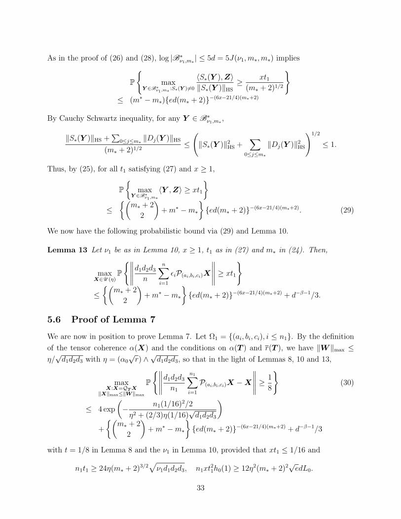
Here ⌊x⌋ stands for the integer part of x. Our results on third order tensor then suggests a
sample size requirement of
n ≍ dN/2polylog(d).
This is to be compared with a matricization approach that unfolds an Nth order tensor to
a (nearly) square matrix (see, e.g., Mu et al., 2013) – where the sample size requirement
is d⌈N/2⌉polylog(d). It is interesting to notice that, in this special case, unfolding a higher
order tensor to a third order tensor is preferable to matricization when N is odd.
The main focus of this article is to provide a convex solution to tensor completion that
yields a tighter sample size requirement than those based upon matricization. Although the
nuclear norm minimization we studied is convex, an efficient implementation has so far eluded
us. Indeed, as recently shown by Hillar and Lim (2011), most common tensor problems are
NP hard, including computing the tensor spectral or nuclear norm as we defined. However,
one should interpret such pessimistic results with caution. First of all, NP-hardness does
not rule out the possibility of efficient ways to approximate it. One relevant example is
tensor decomposition, a problem very much related to our approach here. Although also a
NP hard problem in general, there are many algorithms that can do tensor decomposition
efficiently in practice. Moreover, the NP hardness result is for evaluating spectral norm of
an arbitrary tensor. Yet for our purposes, we may only need to do so for a smaller class of
tensors, particularly those in a neighborhood around the truth. It is possible that evaluating
tensor norm in a small neighborhood around the truth can be done in polynomial time. One
such example can actually be easily deducted from Lemma 3 of our manuscript, where we
show that for bi-orthogonal tensors, nuclear norm can be evaluated in polynomial time.
The research on tensor completion is still in its infancy. In addition to the computational
challenges, there are a lot of important questions yet to be addressed. For example, it
is recently shown by Mu et al. (2013) that exact recovery is possible with sample size
requirement of the order (r3 + rd)polylog(d) through direct rank minimization. It remains
unclear whether or not such a sample size requirement can be achieved by a convex approach.
Our hope is that the results from the current work may lead to further understanding of
the nature of tensor related issues, and at some point satisfactory answers to such open
problems.
References
Candes, E.J. and Recht, B. (2008), Exact matrix completion via convex optimization,
Foundations of Computational Mathematics, 9, 717-772.
35

Candes, E.J. and Tao, T. (2009), The power of convex relaxation: Near-optimal matrix
completion, IEEE Transactions on Information Theory, 56(5), 2053-2080.
Gandy, S., Recht, B. and Yamada, I. (2011), Tensor completion and low-n-rank tensor
recovery via convex optimization, Inverse Problems, 27(2), 025010.
Gine, E. and Zinn, J. (1984), Some limit theorems for empirical processes, The Annals of
Probability, 12(4), 929-989.
Gross, D. (2011), Recovering low-rank matrices from few coefficients in any basis, IEEE
Transaction on Information Theory, 57, 1548-1566.
Hillar, C. and Lim, L.H. (2013), Most tensor problems are NP-hard, Journal of the ACM,
60(6), Art. 45.
Kolda, T.G. and Bader, B.W. (2009), Tensor decompositions and applications, SIAM Review,
51(3), 455-500.
Kruskal, J. B. (1989), Rank, decomposition, and uniqueness for 3-way and N-way arrays, in
“Multiway data analysis”, North-Holland, Amsterdam, pp. 7-18.
Li, N. and Li, B. (2010), Tensor completion for on-board compression of hyperspectral
images, In Image Processing (ICIP), 2010 17th IEEE International Conference on, 517-
520.
Liu, J., Musialski, P., Wonka, P. and Ye, J. (2009), Tensor completion for estimating missing
values in visual data, In ICCV, 2114-2121.
Mu, C., Huang, B., Wright, J. and Goldfarb, D. (2013), Square deal: lower bounds and
improved relaxations for tensor recovery, arXiv: 1307.5870.
Recht, B. (2011), A simpler approach to matrix completion, Journal of Machine Learning
Research, 12, 3413-3430.
Semerci, O., Hao, N., Kilmer, M. and Miller, E. (2013), Tensor based formulation and nuclear
norm regularizatin for multienergy computed tomography, to appear in IEEE Transactions
on Image Processing.
Sidiropoulos N.D. and Nion, N. (2010), Tensor algebra and multi-dimensional harmonic
retrieval in signal processing for mimo radar, IEEE Trans. on Signal Processing, 58(11),
5693-5705.
36
Signoretto, M., De Lathauwer, L. and Suykens, J. (2010), Nuclear norms for tensors and
their use for convex multilinear estimation.
Signoretto, M., Van de Plas, R., De Moor, B. and Suykens, J. (2011), Tensor versus matrix
completion: A comparison with application to spectral data, IEEE SPL, 18(7), 403-406.
Tomioka, R., Hayashi, K. and Kashima, H. (2010), Estimation of low-rank tensors via convex
optimization, arXiv preprint arXiv:1010.0789.
Tomioka, R., Suzuki, T., Hayashi, K. and Kashima, H. (2011), Statistical performance of
convex tensor decomposition, Advances in Neural Information Processing Systems (NIPS),
137.
Tropp, J. (2012), User-friendly tail bounds for sums of random matrices, Foundations of
Computational Mathematics, 12, 389-434.
Watson, G. A. (1992), Characterization of the subdifferential of some matrix norms. Linear
Algebra Appl., 170, 33-45.
37


![Convex Coupled Matrix and Tensor Completion …arXiv:1705.05197v2 [stat.ML] 14 Jun 2018 Convex Coupled Matrix and Tensor Completion Kishan Wimalawarne Bioinformatics Center, Institute](https://img.pdfslide.us/doc/110x75/5e60bc431036ec2ab9156b98/convex-coupled-matrix-and-tensor-completion-arxiv170505197v2-statml-14-jun.jpg)