Embed Size (px)
Citation preview
Tensor Calculus
Taha Sochi∗
October 17, 2016
∗Department of Physics & Astronomy, University College London, Gower Street, London, WC1E 6BT.
Email: [email protected].
1
arX
iv:1
610.
0434
7v1
[m
ath.
HO
] 1
4 O
ct 2
016
2
Preface
These notes are the second part of the tensor calculus documents which started with the
previous set of introductory notes [11]. In the present text, we continue the discussion of
selected topics of the subject at a higher level expanding, when necessary, some topics and
developing further concepts and techniques. The purpose of the present text is to solidify,
generalize, fill the gaps and make more rigorous what have been presented in the previous
set of notes and to prepare the ground for the next set of notes. Unlike the previous
notes which are largely based on a Cartesian approach, the present notes are essentially
based on assuming an underlying general curvilinear coordinate system. We also provide a
small sample of proofs to familiarize the reader with the tensor techniques inline with the
tutorial nature of the present text; however, due to the limited objectives of the present
text we do not provide comprehensive proofs and complete theoretical foundations for the
provided materials.
We generally follow the same conventions and notations used in the previous set of notes
with the following amendments:
• We use capital Gamma, Γijk, for the Christoffel symbols of the second kind which is
more elegant and readable than the curly bracket notation{ijk
}that we used in the
previous notes insisting that, despite the suggestive appearance of the Gamma notation,
the Christoffel symbols are not tensors in general.
• Due to the restriction of using real (non-complex) quantities, as stated in the previous
notes, all arguments of real-valued functions, like square roots and logarithmic functions,
are assumed to be non-negative by taking the absolute value, if necessary, without using
the absolute value symbol, as done by some authors. This is to simplify the notation and
avoid confusion with the determinant notation.
•We generalize the partial derivative notation so that ∂i can symbolize the partial deriva-
tive with respect to the ui coordinate of general curvilinear systems and not just for
3
Cartesian coordinates which are usually denoted by xi. The type of coordinates, being
Cartesian or general or otherwise, will be determined by the context which should be
obvious in all cases.
• The summation symbol (i.e.∑
) is used in most cases when a summation is needed but
the summation convention conditions do not apply or there is an ambiguity about it, e.g.
when an index is repeated more than twice or a twice-repeated index is in an upper or
lower state in both positions or a summation index is not repeated visually because it is
part of a squared symbol.
• “Tensor” and “Matrix” are not the same; however for ease of expression they are used
sometimes interchangeably and hence some tensors may be referred to as matrices meaning
the matrix representing the tensor.
• In the present text, all coordinate transformations are assumed to be continuous, single
valued and invertible.
CONTENTS 4
Contents
Preface 2
Contents 4
1 Coordinate Systems, Spaces and Transformations 7
1.1 Coordinate Systems . . . . . . . . . . . . . . . . . . . . . . . . . . . . . . . 7
1.2 Spaces . . . . . . . . . . . . . . . . . . . . . . . . . . . . . . . . . . . . . . 7
1.3 Transformations . . . . . . . . . . . . . . . . . . . . . . . . . . . . . . . . . 9
1.4 Coordinate Surfaces and Curves . . . . . . . . . . . . . . . . . . . . . . . . 13
1.5 Scale Factors . . . . . . . . . . . . . . . . . . . . . . . . . . . . . . . . . . 14
1.6 Basis Vectors in General Curvilinear Systems . . . . . . . . . . . . . . . . 15
1.7 Covariant, Contravariant and Physical Representations . . . . . . . . . . . 19
2 Special Tensors 22
2.1 Kronecker Tensor . . . . . . . . . . . . . . . . . . . . . . . . . . . . . . . . 22
2.2 Permutation Tensor . . . . . . . . . . . . . . . . . . . . . . . . . . . . . . . 23
2.3 Metric Tensor . . . . . . . . . . . . . . . . . . . . . . . . . . . . . . . . . . 26
2.3.1 Dot Product . . . . . . . . . . . . . . . . . . . . . . . . . . . . . . . 32
2.3.2 Cross Product . . . . . . . . . . . . . . . . . . . . . . . . . . . . . . 34
2.3.3 Line Element . . . . . . . . . . . . . . . . . . . . . . . . . . . . . . 36
2.3.4 Surface Element . . . . . . . . . . . . . . . . . . . . . . . . . . . . . 37
2.3.5 Volume Element . . . . . . . . . . . . . . . . . . . . . . . . . . . . 38
2.3.6 Magnitude of Vector . . . . . . . . . . . . . . . . . . . . . . . . . . 39
2.3.7 Angle Between Vectors . . . . . . . . . . . . . . . . . . . . . . . . . 40
2.3.8 Length of Curve . . . . . . . . . . . . . . . . . . . . . . . . . . . . . 40
CONTENTS 5
3 Covariant and Absolute Differentiation 41
3.1 Christoffel Symbols . . . . . . . . . . . . . . . . . . . . . . . . . . . . . . . 41
3.2 Covariant Derivative . . . . . . . . . . . . . . . . . . . . . . . . . . . . . . 49
3.3 Absolute Derivative . . . . . . . . . . . . . . . . . . . . . . . . . . . . . . . 56
4 Differential Operations 59
4.1 General Curvilinear Coordinate System . . . . . . . . . . . . . . . . . . . . 59
4.1.1 Gradient . . . . . . . . . . . . . . . . . . . . . . . . . . . . . . . . . 59
4.1.2 Divergence . . . . . . . . . . . . . . . . . . . . . . . . . . . . . . . . 61
4.1.3 Curl . . . . . . . . . . . . . . . . . . . . . . . . . . . . . . . . . . . 64
4.1.4 Laplacian . . . . . . . . . . . . . . . . . . . . . . . . . . . . . . . . 65
4.2 General Orthogonal Coordinate System . . . . . . . . . . . . . . . . . . . . 67
4.2.1 Gradient . . . . . . . . . . . . . . . . . . . . . . . . . . . . . . . . . 67
4.2.2 Divergence . . . . . . . . . . . . . . . . . . . . . . . . . . . . . . . . 68
4.2.3 Curl . . . . . . . . . . . . . . . . . . . . . . . . . . . . . . . . . . . 68
4.2.4 Laplacian . . . . . . . . . . . . . . . . . . . . . . . . . . . . . . . . 69
4.3 Cylindrical Coordinate System . . . . . . . . . . . . . . . . . . . . . . . . . 69
4.3.1 Gradient . . . . . . . . . . . . . . . . . . . . . . . . . . . . . . . . . 69
4.3.2 Divergence . . . . . . . . . . . . . . . . . . . . . . . . . . . . . . . . 70
4.3.3 Curl . . . . . . . . . . . . . . . . . . . . . . . . . . . . . . . . . . . 70
4.3.4 Laplacian . . . . . . . . . . . . . . . . . . . . . . . . . . . . . . . . 71
4.4 Spherical Coordinate System . . . . . . . . . . . . . . . . . . . . . . . . . . 71
4.4.1 Gradient . . . . . . . . . . . . . . . . . . . . . . . . . . . . . . . . . 71
4.4.2 Divergence . . . . . . . . . . . . . . . . . . . . . . . . . . . . . . . . 72
4.4.3 Curl . . . . . . . . . . . . . . . . . . . . . . . . . . . . . . . . . . . 72
4.4.4 Laplacian . . . . . . . . . . . . . . . . . . . . . . . . . . . . . . . . 73
CONTENTS 6
5 Tensors in Applications 74
5.1 Riemann Tensor . . . . . . . . . . . . . . . . . . . . . . . . . . . . . . . . . 74
5.1.1 Bianchi identities . . . . . . . . . . . . . . . . . . . . . . . . . . . . 80
5.2 Ricci Tensor . . . . . . . . . . . . . . . . . . . . . . . . . . . . . . . . . . . 81
5.3 Einstein Tensor . . . . . . . . . . . . . . . . . . . . . . . . . . . . . . . . . 83
5.4 Infinitesimal Strain Tensor . . . . . . . . . . . . . . . . . . . . . . . . . . . 83
5.5 Stress Tensor . . . . . . . . . . . . . . . . . . . . . . . . . . . . . . . . . . 84
5.6 Displacement Gradient Tensors . . . . . . . . . . . . . . . . . . . . . . . . 85
5.7 Finger Strain Tensor . . . . . . . . . . . . . . . . . . . . . . . . . . . . . . 86
5.8 Cauchy Strain Tensor . . . . . . . . . . . . . . . . . . . . . . . . . . . . . . 86
5.9 Velocity Gradient Tensor . . . . . . . . . . . . . . . . . . . . . . . . . . . . 87
5.10 Rate of Strain Tensor . . . . . . . . . . . . . . . . . . . . . . . . . . . . . . 87
5.11 Vorticity Tensor . . . . . . . . . . . . . . . . . . . . . . . . . . . . . . . . . 88
References 90
1 COORDINATE SYSTEMS, SPACES AND TRANSFORMATIONS 7
1 Coordinate Systems, Spaces and Transformations
• The focus of this section is coordinate systems, their types and transformations as well
as some general properties of spaces which are needed for the development of the concepts
and techniques of tensor calculus in the present and forthcoming notes.
1.1 Coordinate Systems
• In simple terms, a coordinate system is a mathematical device, essentially of geometric
nature, used by an observer to identify the location of points and objects and describe
events in generalized space which may include space-time.
• The coordinates of a system can have the same or different physical dimensions. An
example of the first is the Cartesian system where all the coordinates have the dimension
of length, while examples of the second include the cylindrical and spherical systems where
some coordinates have the dimension of length while others are dimensionless.
• Generally, the physical dimensions of the components and basis vectors of the covariant
and contravariant forms of a tensor are different.
1.2 Spaces
• A Riemannian space is a manifold characterized by the existing of a symmetric rank-2
tensor called the metric tensor. The components of this tensor, which can be in covariant
(gij) or contravariant (gij) forms, are in general continuous variable functions of coordi-
nates, i.e. gij = gij(u1, u2, . . . , un) and gij = gij(u1, u2, . . . , un) where ui symbolize general
coordinates. This tensor facilitates, among other things, the generalization of lengths and
distances in general coordinates where the length of an element of arc, ds, is defined by:
(ds)2 = gijduiduj (1)
1.2 Spaces 8
In the special case of a Euclidean space coordinated by a rectangular system, the metric
becomes the identity tensor, that is:
gij = gij = gij = δij = δij = δij (2)
• The metric of a Riemannian space may be called the Riemannian metric. Similarly, the
geometry of the space may be described as a Riemannian geometry.
• All spaces dealt with in the present notes are Riemannian with well-defined metrics.
• A manifold or space is dubbed “flat” when it is possible to find a coordinate system for the
space with a diagonal metric tensor whose all diagonal elements are ±1; the space is called
“curved” otherwise. Examples of flat space are the 3D Euclidean space coordinated by a
rectangular Cartesian system whose metric tensor is diagonal with all the diagonal elements
being +1, and the 4D Minkowski space-time whose metric is diagonal with elements of
±1. Examples of curved space is the 4D space-time of general relativity in the presence
of matter and energy.
• When all the diagonal elements of the metric tensor of a flat space are +1, the space
and the coordinate system may be described as homogeneous.
• An nD manifold is Euclidean iff Rijkl = 0 where Rijkl is the Riemann tensor (see § 5.1);
otherwise the manifold is curved to which the general Riemannian geometry applies.
• A “field” is a function of the position vector over a region of space. Scalars, vectors
and tensors may be defined on a single point of the space or over an extended region
of the space; in the latter case we have scalar fields, vector fields and tensor fields, e.g.
temperature field, velocity field and stress field respectively.
• In metric spaces, the physical quantities are independent of the form of description, being
covariant or contravariant, as the metric tensor facilitates the transformation between the
different forms; hence making the description objective.
1.3 Transformations 9
1.3 Transformations
• In general terms, a transformation from an nD space to another nD space is a corre-
lation that maps a point from the first space (original) to a point in the second space
(transformed) where each point in the original and transformed spaces is identified by n
independent variables or coordinates. To distinguish between the two sets of coordinates
in the two spaces, the coordinates of the points in the transformed space may be notated
with barred symbols, e.g. (u1, u2, . . . , un) or (u1, u2, . . . , un) where the superscripts and
subscripts are indices, while the coordinates of the points in the original space are notated
with unbarred similar symbols, e.g. (u1, u2, . . . , un) or (u1, u2, . . . , un). Under certain
conditions, which will be clarified later, such a transformation is unique and hence an
inverse transformation from the transformed space to the original space is also defined.
Mathematically, each one of the direct and inverse transformations can be regarded as
a correlation expressed by a set of equations in which each coordinate in one space is
considered as a function of the coordinates in the other space. Hence the transformations
between the two sets of coordinates in the two spaces can by expressed mathematically by
the following two sets of independent relations:
ui = ui(u1, u2, . . . , un) & ui = ui(u1, u2, . . . , un) (3)
where i = 1, 2, . . . , n with n being the space dimension. The independence of the above
relations is guaranteed iff the Jacobian of the transformation does not vanish on any point
in the space (see about Jacobian the forthcoming points). An alternative to viewing the
transformation as a mapping between two different spaces is to view it as a correlation
of the same point in the same space but observed from two different coordinate frames
of reference which are subject to a similar transformation. The following points will be
largely based on the latter view.
1.3 Transformations 10
• As far as the notation is concerned, there is no fundamental difference between the
barred and unbarred systems and hence the notation can be interchanged.
• An injective transformation maps any two distinct points of the original space, r1 and
r2, onto two distinct points of the transformed space, r1 and r2. The image of an injective
transformation, r, is regarded as coordinates for the point, and the collection of all such
coordinates of the space points may be considered as a representation of a coordinate
system for the space. If the mapping from an original rectangular system is linear, the
coordinate system obtained from such a transformation is called “affine”. Coordinate
systems which are not affine are described as “curvilinear” such as cylindrical and spherical
systems.
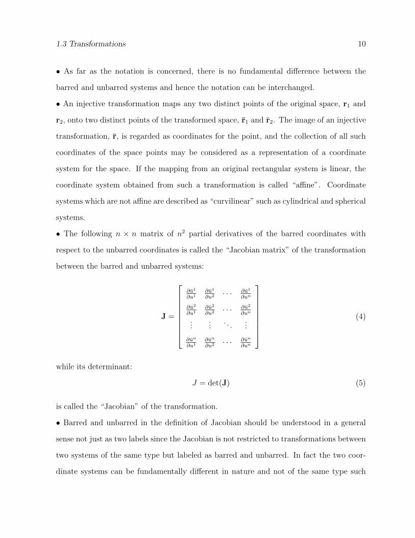
• The following n × n matrix of n2 partial derivatives of the barred coordinates with
respect to the unbarred coordinates is called the “Jacobian matrix” of the transformation
between the barred and unbarred systems:
J =
∂u1
∂u1∂u1
∂u2· · · ∂u1
∂un
∂u2
∂u1∂u2
∂u2· · · ∂u2
∂un
......
. . ....
∂un
∂u1∂un
∂u2· · · ∂un
∂un
(4)
while its determinant:
J = det(J) (5)
is called the “Jacobian” of the transformation.
• Barred and unbarred in the definition of Jacobian should be understood in a general
sense not just as two labels since the Jacobian is not restricted to transformations between
two systems of the same type but labeled as barred and unbarred. In fact the two coor-
dinate systems can be fundamentally different in nature and not of the same type such
1.3 Transformations 11
as Cartesian and general curvilinear. The Jacobian matrix and determinant represent
any transformation by the above partial derivative matrix system between two coordi-
nates defined by two different sets of coordinate variables not necessarily as barred and
unbarred. The objective of defining the Jacobian as between barred and unbarred systems
is generality and clarity.
• The transformation from the unbarred coordinate system to the barred coordinate system
is bijective1 iff J 6= 0 on any point in the transformed region of the space. In this case
the inverse transformation from the barred to the unbarred system is also defined and
bijective and is represented by the inverse of the Jacobian matrix:2
J = J−1 (6)
Consequently, the Jacobian of the inverse transformation, being the determinant of the
inverse Jacobian matrix, is the reciprocal of the Jacobian of the original transformation:
J =1
J(7)
• A coordinate transformation is admissible iff the transformation is bijective with non-
vanishing Jacobian and the transformation function is of class C2.3
• “Affine tensors” are tensors that correspond to admissible linear coordinate transforma-
tions from an original rectangular system of coordinates.
• Coordinate transformations are described as “proper” when they preserve the handed-
1Bijective transformation means injective (one-to-one) and surjective (onto) mapping.2Notationally, there is no fundamental difference between the barred and unbarred systems and hence
the labeling is rather arbitrary and can be interchanged. Therefore, the Jacobian may be notated asbarred over unbarred or the other way around. Yes, in a specific context when one of these is labeledas the Jacobian, the other one should be labeled as the inverse Jacobian to distinguish between the twoopposite Jacobians and their corresponding transformations.
3Cn continuity condition means that the function and all its first n partial derivatives do exist andare continuous in their domain of definition. Also, some authors impose a weaker condition of being ofclass C1.
1.3 Transformations 12
ness (right- or left-handed) of the coordinate system and “improper” when they reverse
the handedness. Improper transformations involve an odd number of coordinate axes
inversions through the origin.
• Inversion of axes may be called improper rotation while ordinary rotation is described
as proper rotation.
• Transformations of coordinates can be active, when they change the state of the observed
object such as rotating the object in the space, or passive when they are based on keeping
the state of the object and changing the state of the coordinate system which the object
is observed from. In brief, the subject of an active transformation is the object while the
subject of a passive transformation is the coordinate system.
• An object that does not change by admissible coordinate transformations is described
as “invariant” such as the value of a true scalar and the length of a vector.
• As there are essentially two different types of basis vectors, namely tangent vectors of
covariant nature and gradient vectors of contravariant nature, there are two main types
of non-scalar tensors: contravariant and covariant tensors which are based on the type
of the employed basis vectors. Tensors of mixed type employ in their definition mixed
basis vectors of the opposite type to the corresponding indices of their components. As
indicated earlier, the transformation between these different types is facilitated by the
metric tensor.
• A product or composition of coordinate transformations is a succession of transforma-
tions where the output of one transformation is taken as the input to the next transfor-
mation. In such cases, the Jacobian of the product is the product of the Jacobians of the
individual transformations of which the product is made.
• The collection of all admissible coordinate transformations with non-vanishing Jacobian
form a group, that is they satisfy the properties of closure, associativity, identity and
inverse. Hence, any convenient admissible coordinate system can be chosen as the point
1.4 Coordinate Surfaces and Curves 13
of entry since other systems can be reached, if needed, through the set of admissible
transformations. This is the cornerstone of building covariant physical theories which are
independent of the subjective choice of coordinate systems and reference frames.
• Transformation of coordinates is not a commutative operation.
1.4 Coordinate Surfaces and Curves
• The surfaces of constant coordinates at a certain point of the space meet to form curves
(i.e. curves of intersection of these surfaces in pairs). The coordinate curves are these
curves of mutual intersection of the surfaces of constant coordinates of the curvilinear
system.
• The above transformation equations (Eq. 3) are used to define the set of surfaces of
constant coordinates and coordinate curves of mutual intersection of these surfaces. These
coordinate surfaces and curves play a crucial role in the formulation and development of
this subject.
• The coordinate axes of a coordinate system can be rectilinear, and hence the coordinate
curves are straight lines and the surfaces of constant coordinates are planes, as in the
case of rectangular Cartesian systems, or curvilinear, and hence the coordinate curves are
generalized curved paths and the surfaces of constant coordinates are generalized curved
surfaces, as in the case of cylindrical and spherical systems.
• In curvilinear coordinate systems, some or all of the coordinate surfaces are not planes
and some or all of the coordinate lines are not straight lines.
• Orthogonal coordinate systems are those for which the vectors tangent to the coordinate
curves, as well as the vectors normal to the surfaces of constant coordinates, are mutually
perpendicular at all points of the space. Consequently, in orthogonal coordinates, the coor-
dinate surfaces are mutually perpendicular and the coordinate lines are also perpendicular
at the point of intersection.
1.5 Scale Factors 14
• In orthogonal coordinate systems, the corresponding covariant and contravariant basis
vectors at any given point in the space are in the same direction, i.e. the tangent vector
to a particular coordinate curve ui at a certain point and the gradient vector normal to
the surface of constant ui at the same point have the same direction although they may
be of different length.
• A necessary and sufficient condition for a coordinate system to be orthogonal is that its
metric tensor is diagonal.
• An admissible coordinate transformation from a Cartesian system defines another Carte-
sian system if the transformation is linear, and defines a curvilinear system if the trans-
formation is nonlinear.
1.5 Scale Factors
• Scale factors (usually symbolized with h1, h2, . . . hn) of a coordinate system are those
factors which are required to multiply the coordinate differentials to obtain distances
traversed during a change in the coordinate of that magnitude, e.g. ρ in the plane polar
coordinate system which multiplies the differential of the polar angle dφ to obtain the
distance L traversed by a change of magnitude dφ in the polar angle which is L = ρ dφ.
They are also used to normalize the basis vectors (refer to the previous notes [11] and
forthcoming notes).
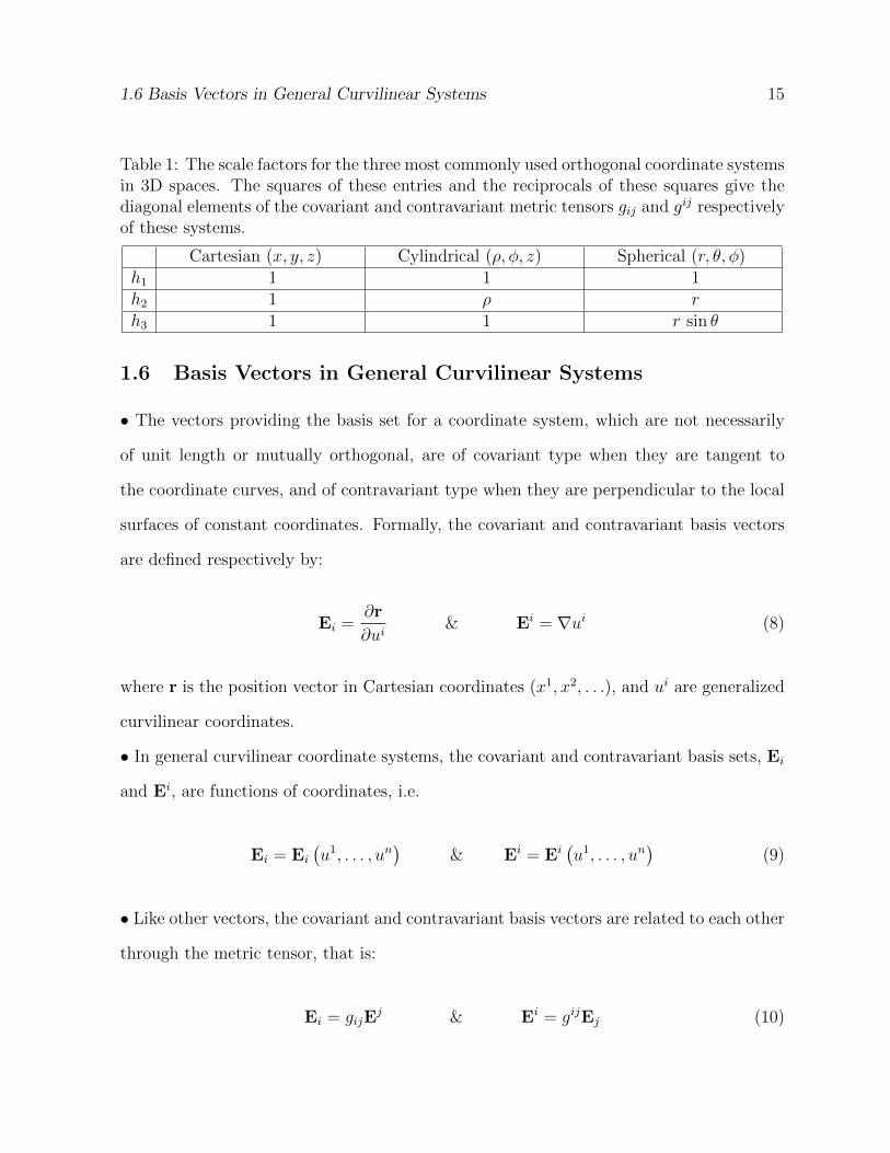
• The scale factors for the Cartesian, cylindrical and spherical coordinate systems in 3D
spaces are given in Table 1.
• The scale factors are also used in the expressions for the differential elements of arc,
surface and volume in general orthogonal coordinates, as described in § 2.3.
1.6 Basis Vectors in General Curvilinear Systems 15
Table 1: The scale factors for the three most commonly used orthogonal coordinate systemsin 3D spaces. The squares of these entries and the reciprocals of these squares give thediagonal elements of the covariant and contravariant metric tensors gij and gij respectivelyof these systems.
Cartesian (x, y, z) Cylindrical (ρ, φ, z) Spherical (r, θ, φ)h1 1 1 1h2 1 ρ rh3 1 1 r sin θ
1.6 Basis Vectors in General Curvilinear Systems
• The vectors providing the basis set for a coordinate system, which are not necessarily
of unit length or mutually orthogonal, are of covariant type when they are tangent to
the coordinate curves, and of contravariant type when they are perpendicular to the local
surfaces of constant coordinates. Formally, the covariant and contravariant basis vectors
are defined respectively by:
Ei =∂r
∂ui& Ei = ∇ui (8)
where r is the position vector in Cartesian coordinates (x1, x2, . . .), and ui are generalized
curvilinear coordinates.
• In general curvilinear coordinate systems, the covariant and contravariant basis sets, Ei
and Ei, are functions of coordinates, i.e.
Ei = Ei
(u1, . . . , un
)& Ei = Ei
(u1, . . . , un
)(9)
• Like other vectors, the covariant and contravariant basis vectors are related to each other
through the metric tensor, that is:
Ei = gijEj & Ei = gijEj (10)
1.6 Basis Vectors in General Curvilinear Systems 16
• The covariant and contravariant basis vectors are reciprocal basis systems, and hence
in a 3D space with a right-handed coordinate system (u1, u2, u3) they are linked by the
following relations:
E1 =E2 × E3
E1 · (E2 × E3), E2 =
E3 × E1
E1 · (E2 × E3), E3 =
E1 × E2
E1 · (E2 × E3)(11)
E1 =E2 × E3
E1 · (E2 × E3), E2 =
E3 × E1
E1 · (E2 × E3), E3 =
E1 × E2
E1 · (E2 × E3)(12)
• The relations in the last point may be expressed in a more compact form as follow:
Ei =Ej × Ek
Ei · (Ej × Ek)& Ei =
Ej × Ek
Ei · (Ej × Ek)(13)
where i, j, k take respectively the values 1, 2, 3 and the other two cyclic permutations (i.e.
2, 3, 1 and 3, 1, 2).
• The magnitude of the scalar triple product Ei · (Ej × Ek) represents the volume of the
parallelepiped formed by Ei, Ej and Ek.
• The magnitudes of the basis vectors in general orthogonal coordinates are given by:
|Ei| = hi &∣∣Ei∣∣ =
1
hi(14)
where hi is the scale factor for the ith coordinate.
• The base vectors in the barred and unbarred general curvilinear coordinate systems are
related by the following transformation rules:
Ei =∂uj
∂uiEj & Ei =
∂uj
∂uiEj
Ei =∂ui
∂ujEj & Ei =
∂ui
∂ujEj
(15)
1.6 Basis Vectors in General Curvilinear Systems 17
where the indexed u and u represent the coordinates in the unbarred and barred sys-
tems respectively. The transformation rules for the components can be straightforwardly
concluded from the above rules; for example for a vector A which can be represented
covariantly and contravariantly in the unbarred and barred systems as:
A = EiAi = EiAi
A = EiAi = EiA
i
(16)
the transformation equations of its components between the two systems are given respec-
tively by:
Ai =∂uj
∂uiAj & Ai =
∂uj
∂uiAj
Ai =∂ui
∂ujAj & Ai =
∂ui
∂ujAj
(17)
These transformation rules can be easily extended to higher rank tensors of different
variance types, as detailed in the introductory notes [11].
• For a 3D manifold with a right-handed curvilinear coordinate system, we have:
E1 · (E2 × E3) =√g & E1 ·
(E2 × E3
)=
1√g
(18)
where g is the determinant of the covariant metric tensor, i.e.
g = det (gij) = |gij| (19)
• Because Ei · Ej = gij (Eq. 51) we have:
JTJ = [gij] (20)
where J is the Jacobian matrix transforming between Cartesian and generalized coordi-
nates, the superscript T represents matrix transposition, [gij] is the matrix representing
1.6 Basis Vectors in General Curvilinear Systems 18
the covariant metric tensor and the product on the left is a matrix product as defined in
linear algebra which is equivalent to a dot product in tensor algebra.
• Considering Eq. 20, the relation between the determinant of the metric tensor and the
Jacobian is given by:
g = J2 (21)
where J (=∣∣∂x∂u
∣∣ with x for Cartesian and u for generalized coordinates) is the Jacobian
of the transformation.
• As explained earlier, in orthogonal coordinate systems the covariant and contravariant
basis vectors, Ei and Ei, at any specific point of the space are in the same direction, and
hence the normalization of each one of these basis sets, by dividing each basis vector by
its magnitude, produces identical orthonormal basis sets.4 This, however, is not true in
general curvilinear coordinates where each normalized basis set is different in general from
the other.
• When the covariant basis vectors Ei are mutually orthogonal at all points of the space,
we have:
(A) the contravariant basis vectors Ei are mutually orthogonal as well,
(B) the covariant and contravariant metric tensors, gij and gij, are diagonal with non-
vanishing diagonal elements, i.e.
gij = gij = 0 (i 6= j) (22)
gii 6= 0 & gii 6= 0 (no sum on i) (23)
(C) the diagonal elements of the covariant and contravariant metric tensors are reciprocals,
4Consequently, there is no difference between the covariant and contravariant components of tensorswith respect to such contravariant and covariant orthonormal basis sets.
1.7 Covariant, Contravariant and Physical Representations 19
i.e.5
gii =1
gii(no summation) (24)
(D) the magnitude of the contravariant and covariant basis vectors are reciprocals, i.e.
∣∣Ei∣∣ =
1
|Ei|(25)
1.7 Covariant, Contravariant and Physical Representations
• So far we are familiar with the covariant and contravariant (including mixed) repre-
sentations of tensors. There is still another type of representation, that is the physical
representation which is the common one in the applications of tensor calculus such as fluid
and continuum mechanics.
• The covariant and contravariant basis vectors, as well as the covariant and contravariant
components of a vector, do not in general have the same physical dimensions as indicated
earlier; moreover, the basis vectors may not have the same magnitude. This motivates
the introduction of a more standard form of vectors by using physical components (which
have the same dimensions) with normalized basis vectors (which are dimensionless with
unit magnitude) where the metric tensor and the scale factors are employed to facilitate
this process. The normalization of the basis vectors is done by dividing each vector by its
magnitude. For example, the normalized covariant basis vectors of a general coordinate
system, Ei, are given by:
Ei =Ei
|Ei|(no sum on i) (26)
5The comment “no summation” may not be needed in this type of expressions since both indices areof the same variance type in a generally non-Cartesian system.
1.7 Covariant, Contravariant and Physical Representations 20
which for an orthogonal coordinate system becomes:
Ei =Ei√gii
=Ei
hi(no sum on i) (27)
where gii is the ith diagonal element of the covariant metric tensor and hi is the scale factor
of the ith coordinate as described previously. Consequently if the physical components of
a vector are notated with a hat, then for an orthogonal system we have:
A = AiEi = AiEi = AiEi√gii
=⇒ Ai =√giiA
i = hiAi (no sum) (28)
Similarly for the contravariant basis vectors we have:
A = AiEi = AiE
i = AiEi√gii
=⇒ Ai =√giiAi =
Ai√gii
=Aihi
(no sum)
(29)
where gii is the ith diagonal element of the contravariant metric tensor. These definitions
and processes can be easily extended to tensors of higher ranks.
• The physical components of higher rank tensors are similarly defined as for rank-1 tensors
by considering the basis vectors of the coordinated space where similar simplifications
apply to orthogonal systems with mutually-perpendicular basis vectors. For example, for
a rank-2 tensor A with an orthogonal coordinate system, the physical components can be
represented by:
Aij =Aijhihj
(no sum on i or j, with basis EiEj)
Aij = hihjAij (no sum on i or j, with basis EiEj)
Aij =hiA
ij
hj(no sum on i or j, with basis EiE
j)
(30)
• On generalizing the above pattern, the physical components of a tensor of type (m,n)
1.7 Covariant, Contravariant and Physical Representations 21
in a general orthogonal coordinate system are given by:
Aa1...amb1...bn=ha1 . . . hamhb1 . . . hbn
Aa1...amb1...bn(31)
• As a consequence of the last points, in a space with a well defined metric any tensor
can be expressed in covariant or contravariant (including mixed) or physical forms using
different sets of basis vectors. Moreover, these forms can be transformed from each other
using the raising and lowering operators and scale factors. As before, for the Cartesian
rectangular systems the covariant, contravariant and physical components are the same
where the Kronecker delta is the metric tensor.
• For orthogonal coordinate systems, the two sets of normalized covariant and contravari-
ant basis vectors are identical as established earlier, and hence the physical components
related to the covariant and contravariant components are identical as well. Consequently,
for orthogonal systems with orthonormal basis vectors, the covariant, contravariant and
physical components are identical.
• The physical components of a tensor may be represented by the symbol of the tensor with
subscripts denoting the coordinates of the employed coordinate system. For instance, if A
is a vector in a 3D space with contravariant components Ai or covariant components Ai, its
physical components in Cartesian, cylindrical, spherical and general curvilinear systems
may be denoted by (Ax, Ay, Az), (Aρ, Aφ, Az), (Ar, Aθ, Aφ) and (Au, Av, Aw) respectively.
• For consistency and dimensional homogeneity, the tensors in scientific applications are
normally represented by their physical components with a set of normalized unit base vec-
tors. The invariance of the tensor form then guarantees that the same tensor formulation
is valid regardless of any particular coordinate system where standard tensor transforma-
tions can be used to convert from one form to another without affecting the validity and
invariance of the formulation.
2 SPECIAL TENSORS 22
2 Special Tensors
• The subject of investigation of this section is those tensors that form an essential part of
the tensor calculus theory, namely the Kronecker, the permutation and the metric tensors.
2.1 Kronecker Tensor
• This is a rank-2 symmetric, constant, isotropic tensor in all dimensions.
• It is defined as:
δij = δij = δij = δ ji
1 (i = j)
0 (i 6= j)
(32)
• The generalized Kronecker delta is defined as:
δi1...inj1...jn=
1 [(j1 . . . jn) is even permutation of (i1 . . . in)]
−1 [(j1 . . . jn) is odd permutation of (i1 . . . in)]
0 [repeated j’s]
(33)
It can also be defined by the following n× n determinant:
δi1...inj1...jn=
∣∣∣∣∣∣∣∣∣∣∣∣∣
δi1j1 δi1j2 · · · δi1jn
δi2j1 δi2j2 · · · δi2jn...
.... . .
...
δinj1 δinj2 · · · δinjn
∣∣∣∣∣∣∣∣∣∣∣∣∣(34)
where the δij entries in the determinant are the normal Kronecker deltas as defined by Eq.
32.
• The relation between the rank-n permutation tensor and the generalized Kronecker delta
2.2 Permutation Tensor 23
in an nD space is given by:
εi1i2...in = δ1 2...ni1i2...in
& εi1i2...in = δi1i2...in1 2...n (35)
Hence, the permutation tensor ε may be considered as a special case of the generalized Kro-
necker delta. Consequently the permutation tensor can be written as an n×n determinant
consisting of the normal Kronecker deltas.
• If we define
δijlm = δijklmk (36)
then the well known ε− δ relation (Eq. 45) will take the following form:
δijlm = δilδjm − δimδ
jl (37)
Other identities involving δ and ε can also be formulated in terms of the generalized
Kronecker delta.
2.2 Permutation Tensor
• This tensor has a rank equal to the number of dimensions of the space. Hence, a rank-n
permutation tensor has nn components.
• It is a relative tensor of weight −1 for its covariant form and +1 for its contravariant
form.
• It is isotropic and totally anti-symmetric in each pair of its indices, i.e. it changes sign
on swapping any two of its indices.
• It is a pseudo tensor since it acquires a minus sign under improper orthogonal transfor-
mation of coordinates.
2.2 Permutation Tensor 24
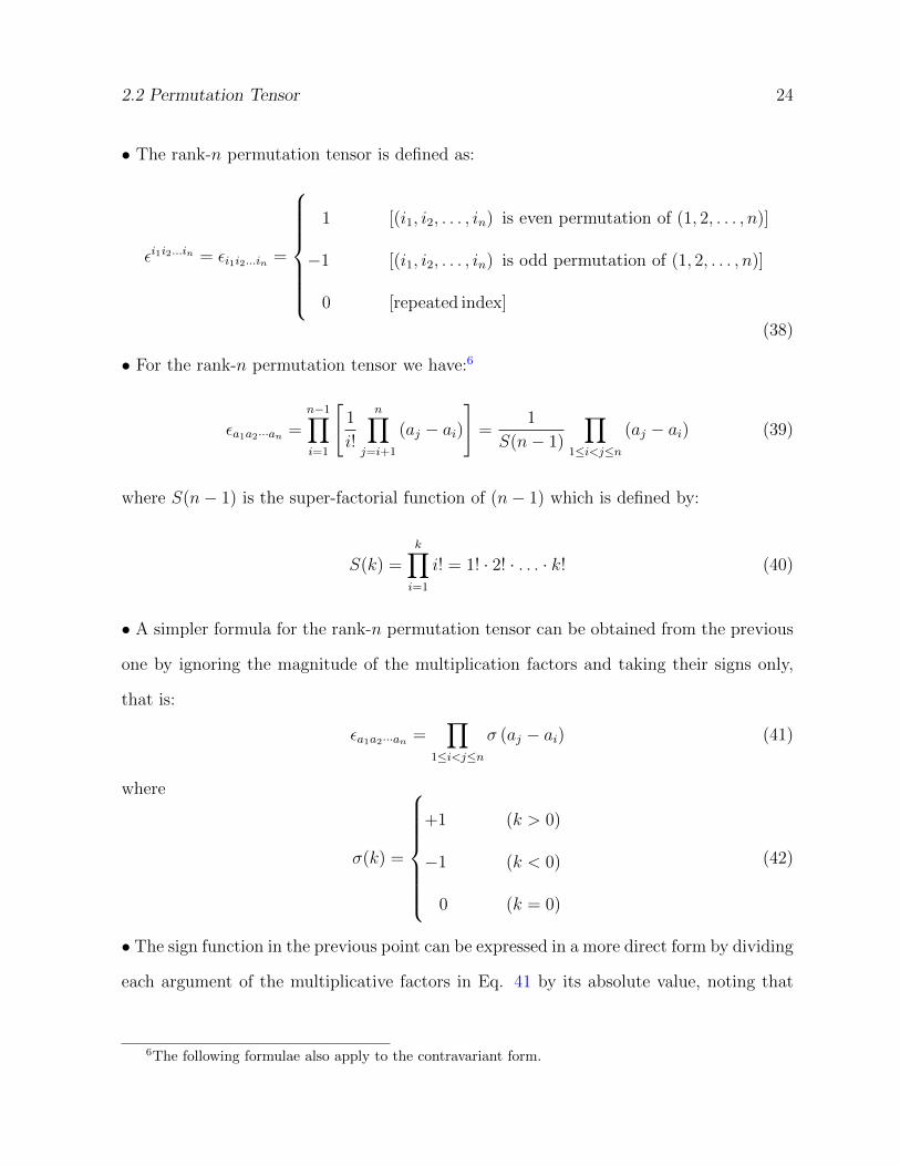
• The rank-n permutation tensor is defined as:
εi1i2...in = εi1i2...in =
1 [(i1, i2, . . . , in) is even permutation of (1, 2, . . . , n)]
−1 [(i1, i2, . . . , in) is odd permutation of (1, 2, . . . , n)]
0 [repeated index]
(38)
• For the rank-n permutation tensor we have:6
εa1a2···an =n−1∏i=1
[1
i!
n∏j=i+1
(aj − ai)
]=
1
S(n− 1)
∏1≤i<j≤n
(aj − ai) (39)
where S(n− 1) is the super-factorial function of (n− 1) which is defined by:
S(k) =k∏i=1
i! = 1! · 2! · . . . · k! (40)
• A simpler formula for the rank-n permutation tensor can be obtained from the previous
one by ignoring the magnitude of the multiplication factors and taking their signs only,
that is:
εa1a2···an =∏
1≤i<j≤n
σ (aj − ai) (41)
where
σ(k) =
+1 (k > 0)
−1 (k < 0)
0 (k = 0)
(42)
• The sign function in the previous point can be expressed in a more direct form by dividing
each argument of the multiplicative factors in Eq. 41 by its absolute value, noting that
6The following formulae also apply to the contravariant form.
2.2 Permutation Tensor 25
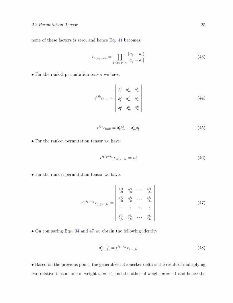
none of these factors is zero, and hence Eq. 41 becomes:
εa1a2···an =∏
1≤i<j≤n
(aj − ai)|aj − ai|
(43)
• For the rank-3 permutation tensor we have:
εijkεlmn =
∣∣∣∣∣∣∣∣∣∣δil δim δin
δjl δjm δjn
δkl δkm δkn
∣∣∣∣∣∣∣∣∣∣(44)
εijkεlmk = δilδjm − δimδ
jl (45)
• For the rank-n permutation tensor we have:
εi1i2···in εi1i2···in = n! (46)
• For the rank-n permutation tensor we have:
εi1i2···in εj1j2···jn =
∣∣∣∣∣∣∣∣∣∣∣∣∣
δi1j1 δi1j2 · · · δi1jn
δi2j1 δi2j2 · · · δi2jn...
.... . .
...
δinj1 δinj2 · · · δinjn
∣∣∣∣∣∣∣∣∣∣∣∣∣(47)
• On comparing Eqs. 34 and 47 we obtain the following identity:
δi1...inj1...jn= εi1...in εj1...jn (48)
• Based on the previous point, the generalized Kronecker delta is the result of multiplying
two relative tensors one of weight w = +1 and the other of weight w = −1 and hence the
2.3 Metric Tensor 26
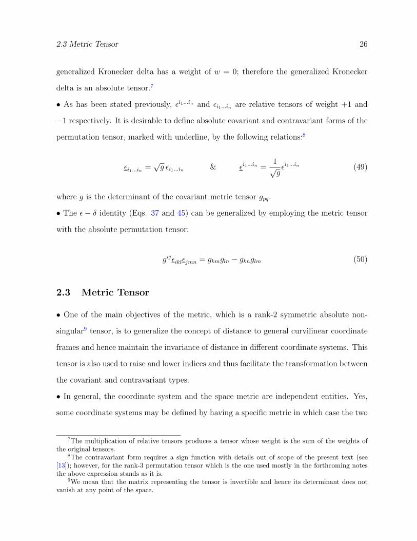
generalized Kronecker delta has a weight of w = 0; therefore the generalized Kronecker
delta is an absolute tensor.7
• As has been stated previously, εi1...in and εi1...in are relative tensors of weight +1 and
−1 respectively. It is desirable to define absolute covariant and contravariant forms of the
permutation tensor, marked with underline, by the following relations:8
εi1...in =√g εi1...in & εi1...in =
1√gεi1...in (49)
where g is the determinant of the covariant metric tensor gpq.
• The ε− δ identity (Eqs. 37 and 45) can be generalized by employing the metric tensor
with the absolute permutation tensor:
gijεiklεjmn = gkmgln − gknglm (50)
2.3 Metric Tensor
• One of the main objectives of the metric, which is a rank-2 symmetric absolute non-
singular9 tensor, is to generalize the concept of distance to general curvilinear coordinate
frames and hence maintain the invariance of distance in different coordinate systems. This
tensor is also used to raise and lower indices and thus facilitate the transformation between
the covariant and contravariant types.
• In general, the coordinate system and the space metric are independent entities. Yes,
some coordinate systems may be defined by having a specific metric in which case the two
7The multiplication of relative tensors produces a tensor whose weight is the sum of the weights ofthe original tensors.
8The contravariant form requires a sign function with details out of scope of the present text (see[13]); however, for the rank-3 permutation tensor which is the one used mostly in the forthcoming notesthe above expression stands as it is.
9We mean that the matrix representing the tensor is invertible and hence its determinant does notvanish at any point of the space.
2.3 Metric Tensor 27
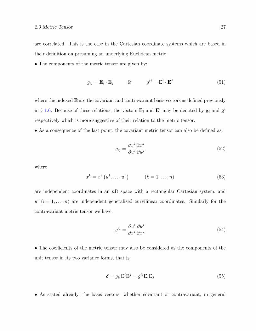
are correlated. This is the case in the Cartesian coordinate systems which are based in
their definition on presuming an underlying Euclidean metric.
• The components of the metric tensor are given by:
gij = Ei · Ej & gij = Ei · Ej (51)
where the indexed E are the covariant and contravariant basis vectors as defined previously
in § 1.6. Because of these relations, the vectors Ei and Ei may be denoted by gi and gi
respectively which is more suggestive of their relation to the metric tensor.
• As a consequence of the last point, the covariant metric tensor can also be defined as:
gij =∂xk
∂ui∂xk
∂uj(52)
where
xk = xk(u1, . . . , un
)(k = 1, . . . , n) (53)
are independent coordinates in an nD space with a rectangular Cartesian system, and
ui (i = 1, . . . , n) are independent generalized curvilinear coordinates. Similarly for the
contravariant metric tensor we have:
gij =∂ui
∂xk∂uj
∂xk(54)
• The coefficients of the metric tensor may also be considered as the components of the
unit tensor in its two variance forms, that is:
δ = gijEiEj = gijEiEj (55)
• As stated already, the basis vectors, whether covariant or contravariant, in general
2.3 Metric Tensor 28
coordinate systems are not necessarily mutually orthogonal and hence the metric tensor
is not diagonal in general since the dot products given in Eqs. 51, 52 and 54 are not
necessarily zero when i 6= j. Moreover, since those basis vectors are not necessarily of unit
length, the entries of the metric tensor are not of unit magnitude in general. However,
since the dot product of vectors is a commutative operation, the metric tensor is necessarily
symmetric.
• The entries of the metric tensor, including the diagonal elements, can be positive or
negative.
• The covariant and contravariant forms of the metric tensor are inverses of each other
and hence:
gikgkj = δij & gikgkj = δ ji (56)
where these equations can be seen as a matrix multiplication (row×column).
• A result from the previous points is that:
(Ei · Ej
)(Ej · Ek) = gijgjk = δik
(Ei · Ej)(Ej · Ek
)= gijg
jk = δ ki
(57)
• As the metric tensor has an inverse, it should not be singular and hence its determinant,
which is in general a function of coordinates like the metric tensor itself, should not vanish
at any point in the space, that is:
g(u1, . . . , un) = det (gij) 6= 0 (58)
• The mixed type metric tensor is given by:
gij = Ei · Ej = δij & g ji = Ei · Ej = δ ji (59)
2.3 Metric Tensor 29
and hence it is the identity tensor. These equations represent the fact that the covariant
and contravariant basis vectors are reciprocal sets.
• From the previous points, it can be concluded that the metric tensor is in fact a trans-
formation of the Kronecker delta in its different variance types from a rectangular system
to a general curvilinear system, that is:
gij =∂xk
∂ui∂xl
∂ujδkl =
∂xk
∂ui∂xk
∂uj= Ei · Ej (covariant)
gij =∂ui
∂xk∂uj
∂xlδkl =
∂ui
∂xk∂uj
∂xk= Ei · Ej (contravariant)
gij =∂ui
∂xk∂xl
∂ujδkl =
∂ui
∂xk∂xk
∂uj= Ei · Ej (mixed)
(60)
• Because of the relations:
Ai = A · Ei = AjEj · Ei = Ajg
ji
Ai = A · Ei = AjEj · Ei = Ajgji
(61)
the metric tensor is used as an operator for raising and lowering indices and hence facili-
tating the transformation between the covariant and contravariant types of vectors. By a
similar argument, the above can be easily generalized where the contravariant metric ten-
sor is used for raising covariant indices and the covariant metric tensor is used for lowering
contravariant indices of tensors of any rank, e.g.
Aik = gijAjk & A kli = gijA
jkl (62)
Consequently, any tensor in a Riemannian space with well-defined metric can be cast into
covariant or contravariant or mixed forms.10
• In the raising and lowering of index operations the metric tensor acts, like a Kronecker
delta, as an index replacement operator as well as shifting the index position.
10For mixed form the rank should be > 1.
2.3 Metric Tensor 30
• In general, the order of the raised and lowered indices is important and hence
gikAjk = A ij and gikAkj = Ai j (63)
are different unless the tensor is symmetric in its two indices, i.e. Ajk = Akj. A dot may
be used to indicate the original position of the shifted index and hence the order of the
indices is recorded, e.g. A ij · and Ai· j for the above examples respectively, although this is
redundant in the case of symmetry.11
• Raising and lowering of indices is a reversible process; hence keeping a record of the
original position of the shifted indices will facilitate the reversal.
• For a space with a coordinate system in which the metric tensor can be cast into a
diagonal form with all the diagonal entries being of unity magnitude (i.e. ±1) the metric
is called flat.
• If g and g are the determinants of the covariant metric tensor in the unbarred and barred
systems respectively, i.e. g = det (gij) and g = det (gij), then
g = J2g &√g = J
√g (64)
where J (=∣∣∂u∂u
∣∣) is the Jacobian of the transformation between the unbarred and barred
systems. Consequently, the determinant of the covariant metric and its square root are
relative scalar invariants of weight +2 and +1 respectively.
• A “conjugate” or “associated” tensor of a tensor in a metric space is a tensor obtained
by inner product multiplication, once or more, of the original tensor by the covariant or
contravariant forms of the metric tensor.
• All tensors associated with a particular tensor through the metric tensor represent the
11Dots may also be inserted in the tensor symbols to remove any ambiguity about the order of theindices even without the action of the raising and lowering operators.
2.3 Metric Tensor 31
same tensor but in different reference frames since the association is no more than raising
or lowering indices by the metric tensor which is equivalent to a representation of the
components of the tensor relative to different basis sets.
• A sufficient and necessary condition for the components of the metric tensor to be
constants in a given coordinate system is that the Christoffel symbols of the first or second
kind vanish identically (refer to 3.1).
• The metric tensor behaves as a constant with respect to covariant and absolute differen-
tiation (see § 3.2 and § 3.3). Hence, in all coordinate systems the covariant and absolute
derivatives of the metric tensor are zero; moreover, the covariant and absolute derivative
operators bypass the metric tensor in differentiating inner and outer products of tensors
involving the metric tensor.
• In general orthogonal coordinate systems in nD spaces the metric tensor and its inverse
are diagonal, that is:
gij = gij = 0 (i 6= j) (65)
moreover, we have:
gii = (hi)2 =
1
gii(no sum on i) (66)
det (gij) = g = g11g22 . . . gnn =∏i
(hi)2 (67)
det(gij)
=1
g=
1
g11g22 . . . gnn=
[∏i
(hi)2
]−1
(68)
where hi (= |Ei|) are the scale factors, as described previously.
• A Riemannian metric, gij, in a particular coordinate system is a Euclidean metric if it
can be transformed to the identity tensor, δij, by a permissible coordinate transformation.
• The Minkowski metric, which is the metric tensor of special relativity, is given by one
2.3.1 Dot Product 32
of the following two forms:
[gij] =[gij]
=
1 0 0 0
0 −1 0 0
0 0 −1 0
0 0 0 −1
[gij] =
[gij]
=
−1 0 0 0
0 1 0 0
0 0 1 0
0 0 0 1
(69)
Consequently, the line element ds can be imaginary.
• The partial derivatives of the covariant and contravariant metric tensors satisfy the
following identities:
∂kgij = −gmjgni∂kgnm
∂kgij = −gmjgin∂kgnm
(70)
• In the following subsections, we investigate a number of mathematical objects whose
definitions and applications are dependent on the metric tensor.
2.3.1 Dot Product
• The dot product of two basis vectors in general curvilinear coordinates was given earlier
in this section. This will be used in the following points to develop expressions for the dot
product of vectors and tensors in general.
• The dot product of two vectors, A and B, in general curvilinear coordinates using their
covariant and contravariant forms, as well as opposite forms, is given by:
A ·B = AiEi ·BjE
j = AiBjEi · Ej = gijAiBj = AjBj = AiB
i
A ·B = AiEi ·BjEj = AiBjEi · Ej = gijAiBj = AjB
j = AiBi (71)
A ·B = AiEi ·BjEj = AiB
jEi · Ej = δijAiBj = AjB
j
A ·B = AiEi ·BjEj = AiBjEi · Ej = δ ji A
iBj = AiBi
2.3.1 Dot Product 33
In brief, the dot product of two vectors is the dot product of their two basis vectors
multiplied algebraically by the algebraic product of their components. Because the dot
product of basis vectors is a metric tensor, the metric tensor will act on the components by
raising or lowering the index of one component or by replacing the index of a component.
• The dot product operations outlined in the previous point can be easily extended to
tensors of higher ranks where the covariant and contravariant forms of the components
and basis vectors are treated in a similar manner to the above to obtain the dot product.
For instance, the dot product of a rank-2 tensor of contravariant components Aij and a
vector of covariant components Bk is given by:
A ·B =(AijEiEj
)·(BkE
k)
= AijBk
(EiEj · Ek
)= AijBkEiδ
kj = AijBjEi (72)
that is, the ith component of this product, which is a contravariant vector, is:
[A ·B]i = AijBj (73)
• From the previous points, the dot product in general curvilinear coordinates occurs
between two vectors of opposite variance type. Therefore, to obtain the dot product of
two vectors of the same variance type, one of the vectors should be converted to the
opposite type by the raising/lowering operator, followed by the inner product operation.
This can be generalized to the dot product of higher-rank tensors where the two contracted
indices of the dot product should be of opposite variance type and hence the index-shifting
operator in the form of the metric tensor should be used, if necessary, to achieve this.
• The generalized dot product of two tensors is an invariant under permissible coordinate
transformations.
2.3.2 Cross Product 34
2.3.2 Cross Product
• The cross product of two covariant basis vectors in general curvilinear coordinates is
given by:
Ei × Ej =∂xl
∂uiel ×
∂xm
∂ujem =
∂xl
∂ui∂xm
∂ujel × em =
∂xl
∂ui∂xm
∂ujεlmnen (74)
where the indexed x and u are the coordinates of Cartesian and general curvilinear sys-
tems respectively, the indexed e are the Cartesian base vectors12 and εlmn = εlmn is the
permutation relative tensor as defined in Eq. 38. Now since en = en = ∂xn
∂ukEk, the last
equation becomes:
Ei × Ej =∂xl
∂ui∂xm
∂uj∂xn
∂ukεlmnE
k = εijkEk (75)
where the underlined absolute covariant permutation tensor is defined as:
εijk =∂xl
∂ui∂xm
∂uj∂xn
∂ukεlmn (76)
So the final result is:
Ei × Ej = εijkEk (77)
By a similar reasoning, we obtain the following expression for the cross product of two
contravariant basis vectors in general curvilinear coordinates:
Ei × Ej = εijkEk (78)
where the absolute contravariant permutation tensor is defined by:
εijk =∂ui
∂xl∂uj
∂xm∂uk
∂xnεlmn (79)
12For Cartesian systems, there is no difference between covariant and contravariant tensors and henceei = ei. We also note that for Cartesian systems g = 1.
2.3.2 Cross Product 35
• Considering Eq. 49, the above equations can also be expressed as:
Ei × Ej = εijkEk =√gεijkE
k (80)
Ei × Ej = εijkEk =εijk√g
Ek (81)
where εijk = εijk are as defined previously (Eq. 38).
• The cross product of non-basis vectors follows similar rules to those outlined above for
the basis vectors; the only difference is that the algebraic product of the components is
used as a scale factor for the cross product of their basis vectors. For example, the cross
product of two contravariant vectors, Ai and Bj, is given by:
A×B =(AiEi
)×(BjEj
)= AiBj (Ei × Ej) = εijkA
iBjEk (82)
that is, the kth component of this product, which is a vector with covariant components,
is:
[A×B]k = εijkAiBj (83)
Similarly, the cross product of two covariant vectors, Ai and Bj, is given by:
A×B =(AiE
i)×(BjE
j)
= AiBj
(Ei × Ej
)= εijkAiBjEk (84)
with the kth contravariant component being given by:
[A×B]k = εijkAiBj (85)
2.3.3 Line Element 36
2.3.3 Line Element
• The displacement differential vector in general curvilinear coordinate systems is given
by:
dr =∂r
∂uidui = Eidu
i =∑i
|Ei|Ei
|Ei|dui =
∑i
|Ei| Eidui (86)
where r is the position vector as defined previously.
• The line element ds, which may also be called the differential of arc length, in general
curvilinear coordinate systems is given by:
(ds)2 = dr · dr = Eidui · Ejdu
j = (Ei · Ej) duiduj = gijdu
iduj (87)
where gij is the covariant metric tensor.
• For orthogonal coordinate systems, the metric tensor is given by:
gij =
0 (i 6= j)
(hi)2 (i = j)
(88)
where hi is the scale factor of the respective coordinate ui. Hence, the last part of Eq. 87
becomes:
(ds)2 =∑i
(hi)2 duidui (89)
with no cross terms (i.e. terms of products involving more than one coordinate like duiduj
where i 6= j) which are generally present in the case of non-orthogonal curvilinear systems.
• On conducting a transformation from one coordinate system to another coordinate
system, marked with barred coordinates, u, the line element will be expressed in the new
system as:
(ds)2 = gijduiduj (90)
2.3.4 Surface Element 37
Since the line element is an invariant quantity, the same symbol (ds)2 is used in both Eqs.
87 and 90.
2.3.4 Surface Element
• In general curvilinear coordinates of a 3D space, an infinitesimal element of area on the
surface u1 = c1, where c1 is a constant, is obtained by taking the magnitude of the cross
product of the displacement vectors in the directions of the other two coordinates on that
surface. Hence, the generalized differential of area element on the surface u1 = c1 is given
by:
dA(u1 = c1) = |dr2 × dr3|
= |E2 × E3| du2du3
=∣∣ε231E
1∣∣ du2du3 (Eq. 77)
= |ε231|∣∣E1∣∣ du2du3
=√g√
E1 · E1 du2du3 (Eqs. 49 & 98)
=√g√g11 du2du3 (Eq. 51)
=√gg11 du2du3
(91)
• On generalizing the above argument, the differential area element in a 3D space on the
surface ui = ci (i = 1, 2, 3) where ci is a constant is given by:
dA(ui = ci) =√ggiidujduk (i 6= j 6= k, no sum on i) (92)
• In general orthogonal coordinates in a 3D space we have:
√ggii =
√(hi)2(hj)2(hk)2
1
(hi)2= hjhk (i 6= j 6= k, no sum on any index) (93)
2.3.5 Volume Element 38
and hence Eq. 92 becomes:
dA(ui = ci) = hjhkdujduk (i 6= j 6= k, no sum on any index) (94)
The last formula represents the area of a surface differential with sides hjduj and hkdu
k
(no sum on j, k).
2.3.5 Volume Element
• In general curvilinear coordinates of a 3D space, an infinitesimal element of volume,
represented by a parallelepiped spanned by the three displacement vectors dri (i = 1, 2, 3),
is obtained by taking the magnitude of the scalar triple product of these vectors. Hence,
the generalized differential volume element is given by:
dV = |dr1 · (dr2 × dr3)|
= |E1 · (E2 × E3)| du1du2du3
=∣∣E1 · ε231E
1∣∣ du1du2du3 (Eq. 77)
=∣∣E1 · E1
∣∣ |ε231| du1du2du3
=∣∣δ 1
1
∣∣ |ε231| du1du2du3 (Eq. 59)
=√g du1du2du3 (Eq. 49)
= J du1du2du3 (Eq. 21)
(95)
where g is the determinant of the covariant metric tensor gij, and J is the Jacobian13 of
the transformation as defined previously. The last line in the last equation is particularly
relevant to the case of change of variables in multivariate integrals where the Jacobian
facilitates the transformation.
13Due to the freedom of choice in the order of the variables, which is related to the choice of the systemhandedness hence affecting the sign of the determinant Jacobian, the sign of the determinant should beadjusted if necessary to have a proper sign for the volume element.
2.3.6 Magnitude of Vector 39
• The formulae in the last point for a 3D space can be extended to the differential of
generalized volume element14 in general curvilinear coordinates in an nD space as follow:
dV =√gdu1 . . . dun = J du1 . . . dun (96)
• In general orthogonal coordinate systems in a 3D space, the above formulae become:
dV = h1h2h3 du1du2du3 (97)
where h1, h2 and h3 are the scale factors. The last formula represents the volume of a
parallelepiped with edges h1du1, h2du
2 and h3du3.
2.3.6 Magnitude of Vector
• The magnitude of a contravariant vector A is given by:
|A| =√
A ·A =√
(Ei · Ej)AiAj =√gijAiAj =
√AjAj =
√AiAi (98)
A similar expression can be obtained for the covariant form of the vector, that is:
|A| =√
A ·A =√
(Ei · Ej)AiAj =√gijAiAj =
√AjAj =
√AiAi (99)
The magnitude of a vector can also be obtained more directly from the dot product of the
covariant and contravariant forms of the vector:
|A| =√
A ·A =√
(Ei · Ej)AiAj =√δijAiA
j =√AiAi =
√AjAj (100)
14Generalized volume elements are used, for instance, to represent the change of variables in multi-variable integrations.
2.3.7 Angle Between Vectors 40
2.3.7 Angle Between Vectors
• The angle θ between two contravariant or two covariant vectors A and B is given
respectively by:
cos θ =A ·B|A| |B|
=gijA
iBj√gklAkAl
√gmnBmBn
=gijAiBj√
gklAkAl√gmnBmBn
(101)
For two vectors of opposite variance type we have:
cos θ =A ·B|A| |B|
=AiBi√
gklAkAl√gmnBmBn
=AiB
i√gklAkAl
√gmnBmBn
(102)
2.3.8 Length of Curve
• In general curvilinear coordinates, the length of a t-parameterized space curve r(t)
defined by ui = ui(t), which represents the distance traversed along the curve on moving
between its start point S and end point E, is given by:15
L =
∫ E
S
√gijduiduj =
∫ t2
t1
√gijdui
dt
duj
dtdt (103)
where t is a scalar variable parameter, and t1 and t2 are the values of t corresponding to
the start and end points respectively.
• The length of curve is used to define the geodesic which is the path of the shortest distance
connecting two points in a Riemannian space. Although the geodesic is a straight line in
a Euclidean space, it is a generalized curved path in a general Riemannian space.
15Some authors add a sign indicator to ensure that the argument of the square root is positive. However,as indicated in the Preface, such a condition is assumed when needed since we deal with non-complexvalues only.
3 COVARIANT AND ABSOLUTE DIFFERENTIATION 41
3 Covariant and Absolute Differentiation
• The focus of this section is the investigation of covariant and absolute differentiation
operations which are closely linked. These operations represent generalization of tensor
differentiation in general curvilinear coordinate systems. Briefly, the differential change
of a tensor in general curvilinear coordinate systems is the result of a change in the
base vectors and a change in the tensor components. Hence, covariant and absolute
differentiation, in place of the normal differentiation, are defined and employed to account
for both of these changes. Since Christoffel symbols are crucial in the formulation and
application of covariant and absolute differentiation, the first subsection of the present
section will be dedicated to these symbols and their properties.
3.1 Christoffel Symbols
• We start by investigating the main properties of the Christoffel symbols which play
crucial roles in tensor calculus in general and are needed for the subsequent development
of the present and forthcoming sections as well as the future notes.
• Christoffel symbols are classified as those of the first kind and those of the second kind.
These two kinds are linked through the index raising and lowering operators. Both kinds
of Christoffel symbols are variable functions of coordinates in general.
• Christoffel symbols of the first and second kind are not tensors in general although they
are affine tensors of rank-3.
• As a consequence of the last point, if all the Christoffel symbols of either kind vanished
in a particular coordinate system they will not necessarily vanish in other systems; for
instance they all vanish in Cartesian systems but not in cylindrical or spherical systems,
as has been established previously [11] and will be investigated further in the forthcoming
points.
3.1 Christoffel Symbols 42
• Christoffel symbols of the first kind are given by:
[ij, l] =1
2(∂jgil + ∂igjl − ∂lgij) (104)
where the indexed g is the covariant form of the metric tensor.
• Christoffel symbols of the second kind are obtained by raising the third index of the
Christoffel symbols of the first kind, that is:
Γkij = gkl [ij, l] =gkl
2(∂jgil + ∂igjl − ∂lgij) (105)
where the indexed g is the metric tensor in its contravariant and covariant forms with
implied summation over l.
• Similarly, the Christoffel symbols of the first kind can be obtained from the Christoffel
symbols of the second kind by reversing the above process through lowering the upper
index, that is:
gkmΓkij = gkmgkl [ij, l] = δlm [ij, l] = [ij,m] (106)
• For an nD space with n covariant basis vectors (E1,E2, . . . ,En) spanning the space, the
derivative ∂jEi for any given i is a vector within the space and hence it is in general a
linear combination of all the basis vectors. The Christoffel symbols of the second kind are
the components of this linear combination, that is:
∂jEi = ΓkijEk (107)
Similarly, for the contravariant basis vectors we have:
∂jEi = −ΓikjE
k (108)
3.1 Christoffel Symbols 43
• By inner product multiplication of the previous relations with the basis vectors we
obtain:
Ei · ∂kEj = Γijk & Ei · ∂kEj = −Γjik (109)
Similarly:
Ek · ∂jEi = gmkEm · ∂jEi = gmkΓ
mij = [ij, k] (110)
• Christoffel symbols of the first and second kind are symmetric in their paired indices,
that is:
[ij, k] = [ji, k] & Γkij = Γkji (111)
• The partial derivative of the components of the covariant metric tensor and the Christof-
fel symbols of the first kind satisfy the following identity, which is essentially based on the
forthcoming Ricci Theorem:
∂jgil = [ij, l] + [jl, i] (112)
This relation can also be written in terms of the Christoffel symbols of the second kind
using the index shifting operator:
∂jgil = gklΓkij + gkiΓ
kjl (113)
A related formula for the partial derivative of the components of the contravariant metric
tensor, which can be obtained by partial differentiation of the relation gimgmj = δji with
respect to the kth coordinate, is given by:
gim∂kgmj = −gmj∂kgim (114)
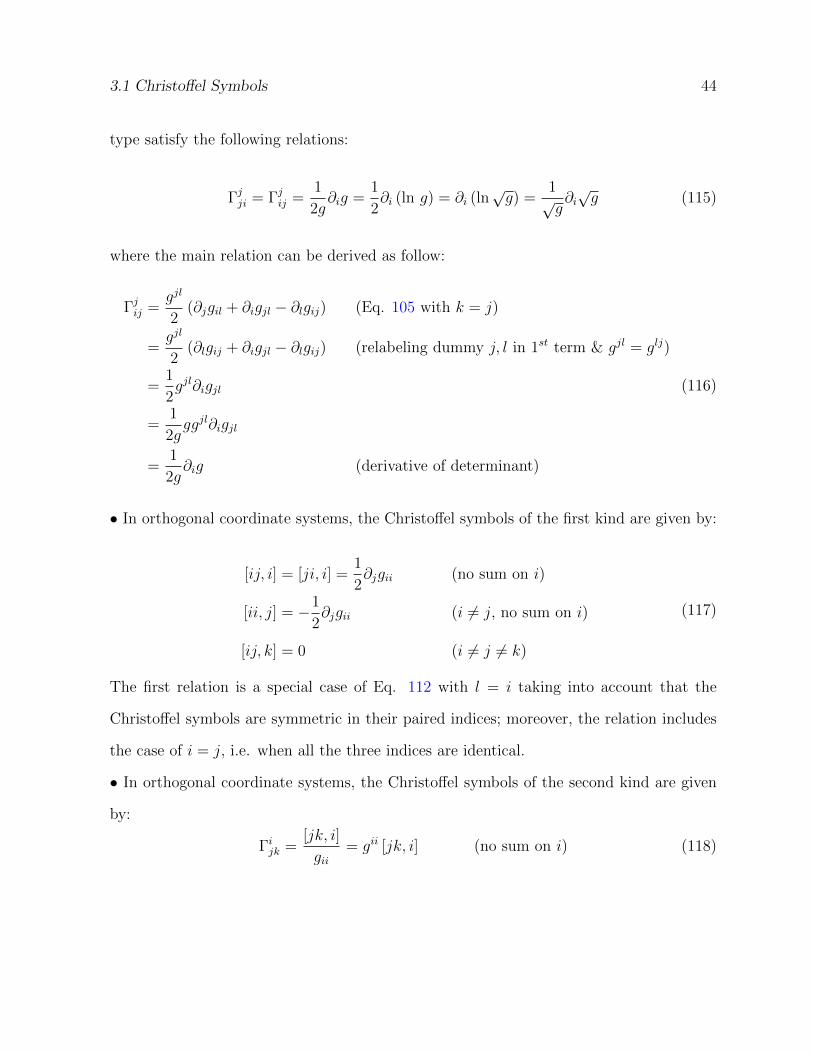
• Christoffel symbols of the second kind with two identical indices of opposite variance
3.1 Christoffel Symbols 44
type satisfy the following relations:
Γjji = Γjij =1
2g∂ig =
1
2∂i (ln g) = ∂i (ln
√g) =
1√g∂i√g (115)
where the main relation can be derived as follow:
Γjij =gjl
2(∂jgil + ∂igjl − ∂lgij) (Eq. 105 with k = j)
=gjl
2(∂lgij + ∂igjl − ∂lgij) (relabeling dummy j, l in 1st term & gjl = glj)
=1
2gjl∂igjl
=1
2gggjl∂igjl
=1
2g∂ig (derivative of determinant)
(116)
• In orthogonal coordinate systems, the Christoffel symbols of the first kind are given by:
[ij, i] = [ji, i] =1
2∂jgii (no sum on i)
[ii, j] = −1
2∂jgii (i 6= j, no sum on i)
[ij, k] = 0 (i 6= j 6= k)
(117)
The first relation is a special case of Eq. 112 with l = i taking into account that the
Christoffel symbols are symmetric in their paired indices; moreover, the relation includes
the case of i = j, i.e. when all the three indices are identical.
• In orthogonal coordinate systems, the Christoffel symbols of the second kind are given
by:
Γijk =[jk, i]
gii= gii [jk, i] (no sum on i) (118)
3.1 Christoffel Symbols 45
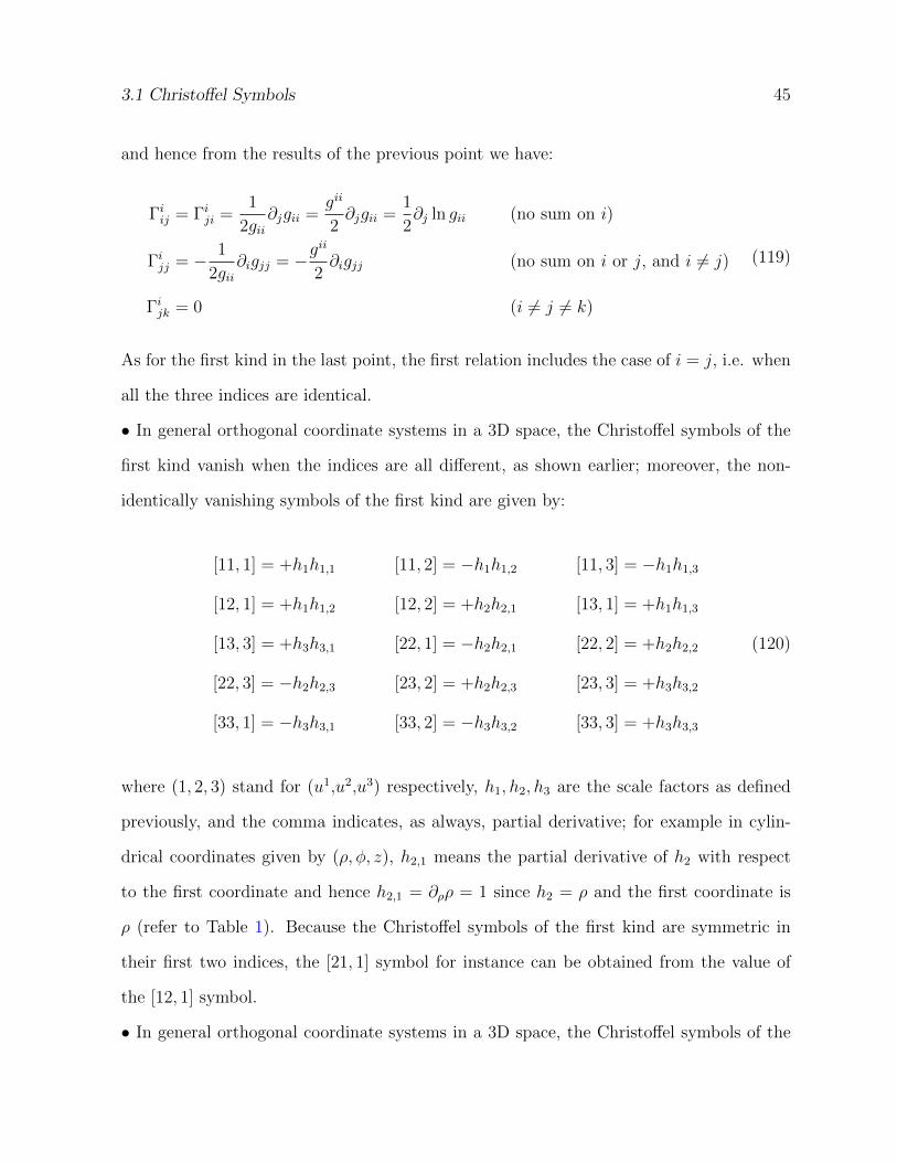
and hence from the results of the previous point we have:
Γiij = Γiji =1
2gii∂jgii =
gii
2∂jgii =
1
2∂j ln gii (no sum on i)
Γijj = − 1
2gii∂igjj = −g
ii
2∂igjj (no sum on i or j, and i 6= j)
Γijk = 0 (i 6= j 6= k)
(119)
As for the first kind in the last point, the first relation includes the case of i = j, i.e. when
all the three indices are identical.
• In general orthogonal coordinate systems in a 3D space, the Christoffel symbols of the
first kind vanish when the indices are all different, as shown earlier; moreover, the non-
identically vanishing symbols of the first kind are given by:
[11, 1] = +h1h1,1 [11, 2] = −h1h1,2 [11, 3] = −h1h1,3
[12, 1] = +h1h1,2 [12, 2] = +h2h2,1 [13, 1] = +h1h1,3
[13, 3] = +h3h3,1 [22, 1] = −h2h2,1 [22, 2] = +h2h2,2 (120)
[22, 3] = −h2h2,3 [23, 2] = +h2h2,3 [23, 3] = +h3h3,2
[33, 1] = −h3h3,1 [33, 2] = −h3h3,2 [33, 3] = +h3h3,3
where (1, 2, 3) stand for (u1,u2,u3) respectively, h1, h2, h3 are the scale factors as defined
previously, and the comma indicates, as always, partial derivative; for example in cylin-
drical coordinates given by (ρ, φ, z), h2,1 means the partial derivative of h2 with respect
to the first coordinate and hence h2,1 = ∂ρρ = 1 since h2 = ρ and the first coordinate is
ρ (refer to Table 1). Because the Christoffel symbols of the first kind are symmetric in
their first two indices, the [21, 1] symbol for instance can be obtained from the value of
the [12, 1] symbol.
• In general orthogonal coordinate systems in a 3D space, the Christoffel symbols of the
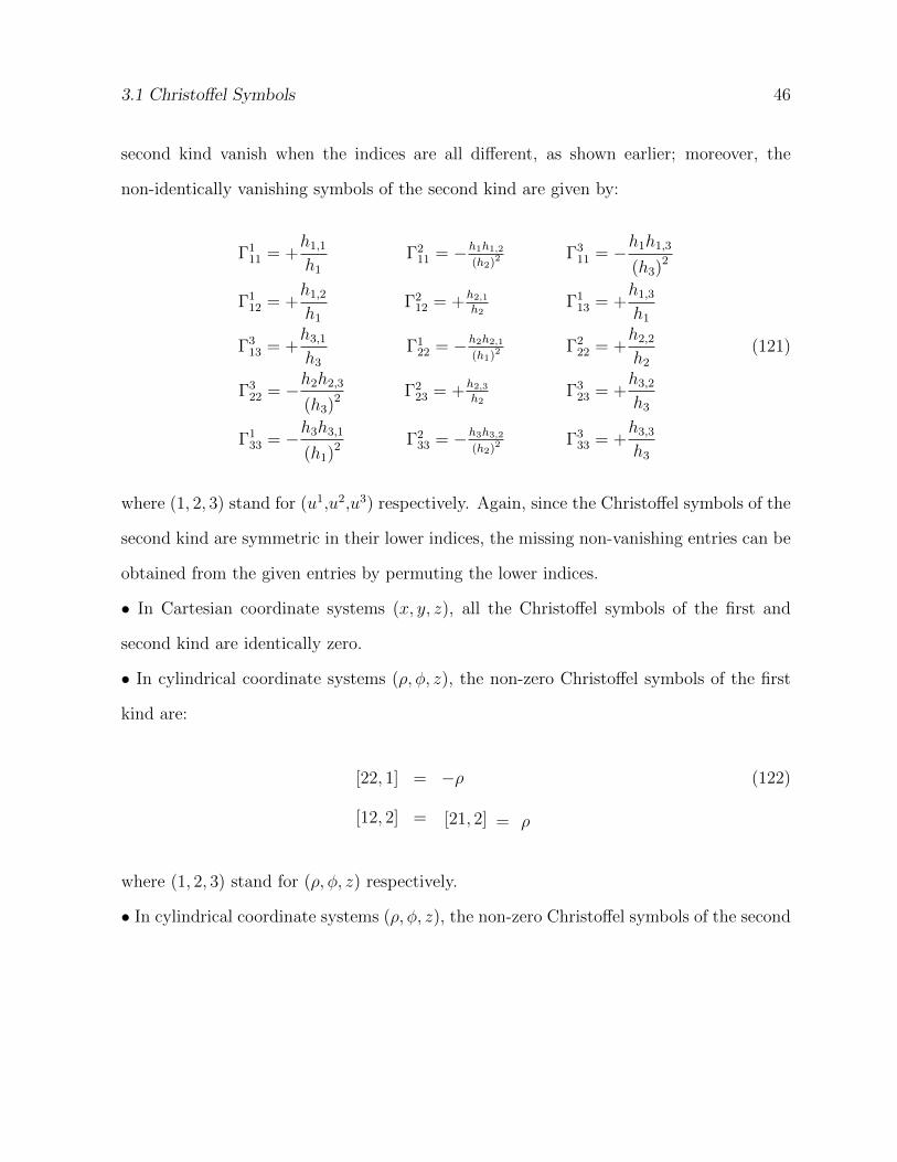
3.1 Christoffel Symbols 46
second kind vanish when the indices are all different, as shown earlier; moreover, the
non-identically vanishing symbols of the second kind are given by:
Γ111 = +
h1,1
h1
Γ211 = −h1h1,2
(h2)2Γ3
11 = −h1h1,3
(h3)2
Γ112 = +
h1,2
h1
Γ212 = +h2,1
h2Γ1
13 = +h1,3
h1
Γ313 = +
h3,1
h3
Γ122 = −h2h2,1
(h1)2Γ2
22 = +h2,2
h2
(121)
Γ322 = −h2h2,3
(h3)2 Γ223 = +h2,3
h2Γ3
23 = +h3,2
h3
Γ133 = −h3h3,1
(h1)2 Γ233 = −h3h3,2
(h2)2Γ3
33 = +h3,3
h3
where (1, 2, 3) stand for (u1,u2,u3) respectively. Again, since the Christoffel symbols of the
second kind are symmetric in their lower indices, the missing non-vanishing entries can be
obtained from the given entries by permuting the lower indices.
• In Cartesian coordinate systems (x, y, z), all the Christoffel symbols of the first and
second kind are identically zero.
• In cylindrical coordinate systems (ρ, φ, z), the non-zero Christoffel symbols of the first
kind are:
[22, 1] = −ρ (122)
[12, 2] = [21, 2] = ρ
where (1, 2, 3) stand for (ρ, φ, z) respectively.
• In cylindrical coordinate systems (ρ, φ, z), the non-zero Christoffel symbols of the second
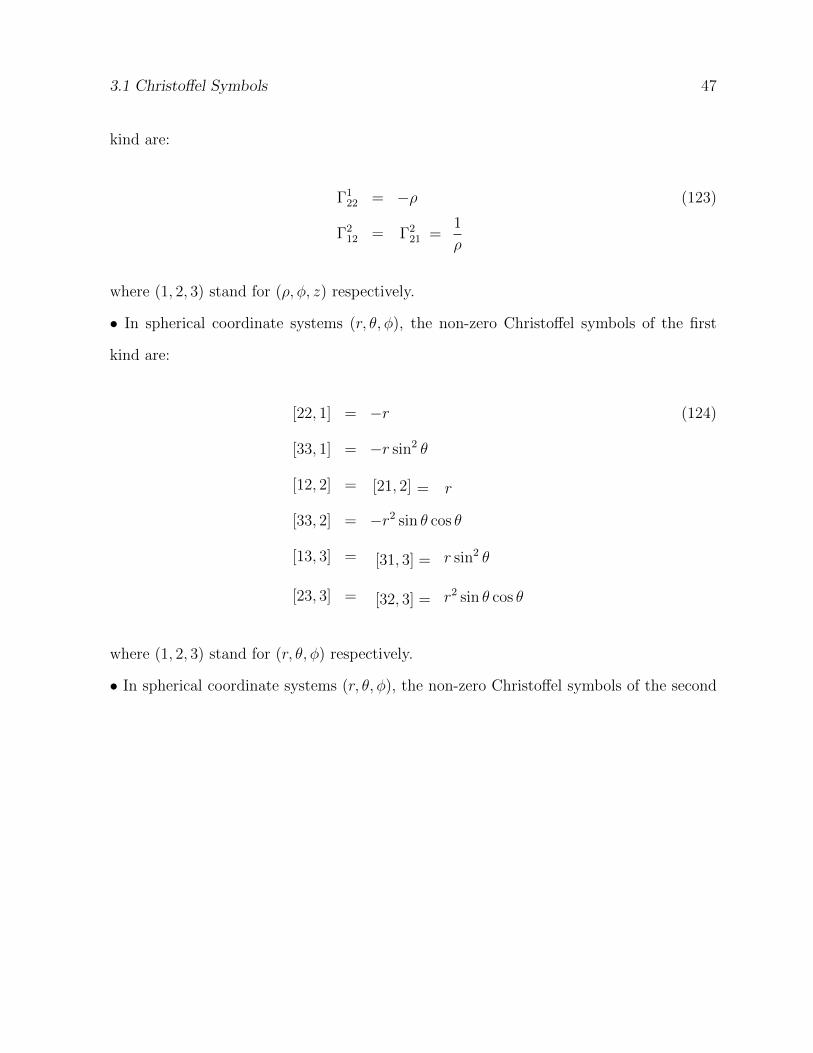
3.1 Christoffel Symbols 47
kind are:
Γ122 = −ρ (123)
Γ212 = Γ2
21 =1
ρ
where (1, 2, 3) stand for (ρ, φ, z) respectively.
• In spherical coordinate systems (r, θ, φ), the non-zero Christoffel symbols of the first
kind are:
[22, 1] = −r (124)
[33, 1] = −r sin2 θ
[12, 2] = [21, 2] = r
[33, 2] = −r2 sin θ cos θ
[13, 3] = [31, 3] = r sin2 θ
[23, 3] = [32, 3] = r2 sin θ cos θ
where (1, 2, 3) stand for (r, θ, φ) respectively.
• In spherical coordinate systems (r, θ, φ), the non-zero Christoffel symbols of the second
3.1 Christoffel Symbols 48
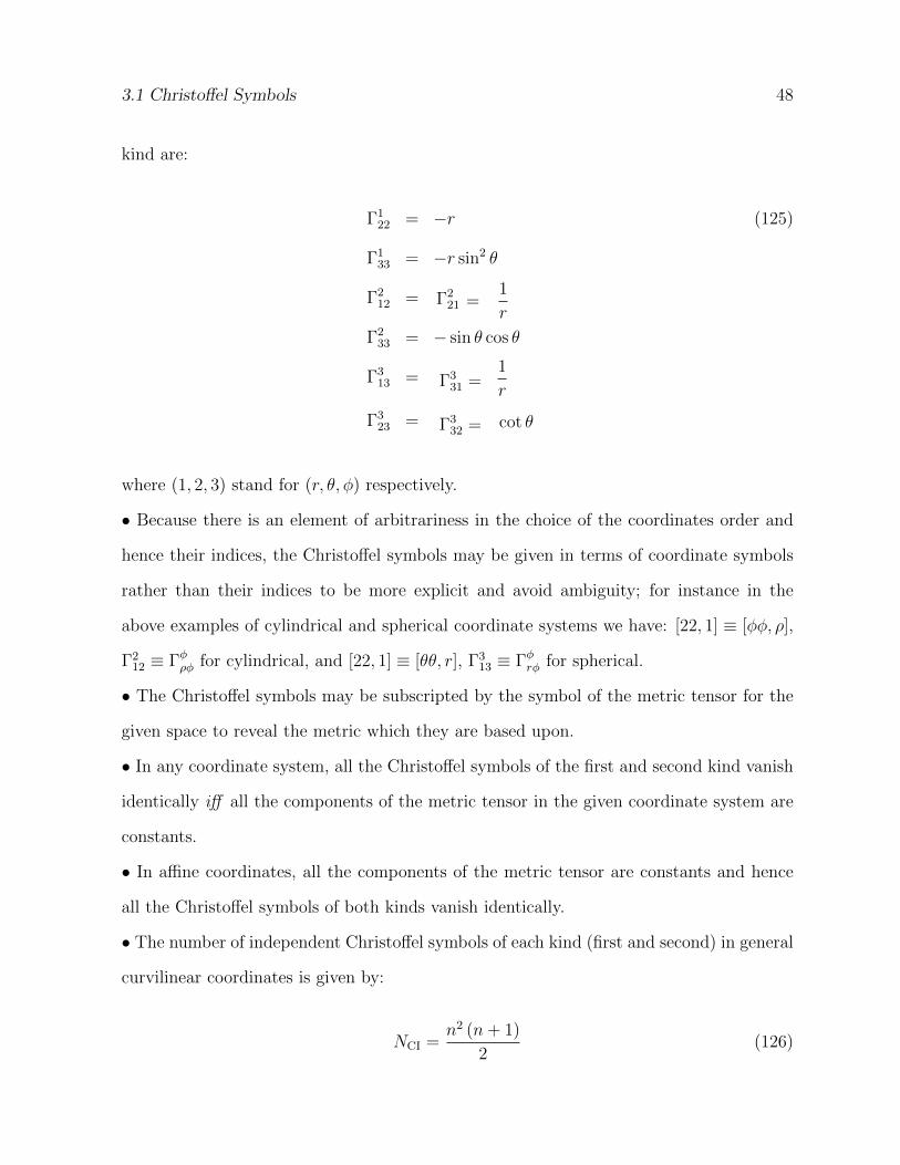
kind are:
Γ122 = −r (125)
Γ133 = −r sin2 θ
Γ212 = Γ2
21 =1
r
Γ233 = − sin θ cos θ
Γ313 = Γ3
31 =1
r
Γ323 = Γ3
32 = cot θ
where (1, 2, 3) stand for (r, θ, φ) respectively.
• Because there is an element of arbitrariness in the choice of the coordinates order and
hence their indices, the Christoffel symbols may be given in terms of coordinate symbols
rather than their indices to be more explicit and avoid ambiguity; for instance in the
above examples of cylindrical and spherical coordinate systems we have: [22, 1] ≡ [φφ, ρ],
Γ212 ≡ Γφρφ for cylindrical, and [22, 1] ≡ [θθ, r], Γ3
13 ≡ Γφrφ for spherical.
• The Christoffel symbols may be subscripted by the symbol of the metric tensor for the
given space to reveal the metric which they are based upon.
• In any coordinate system, all the Christoffel symbols of the first and second kind vanish
identically iff all the components of the metric tensor in the given coordinate system are
constants.
• In affine coordinates, all the components of the metric tensor are constants and hence
all the Christoffel symbols of both kinds vanish identically.
• The number of independent Christoffel symbols of each kind (first and second) in general
curvilinear coordinates is given by:
NCI =n2 (n+ 1)
2(126)
3.2 Covariant Derivative 49
where n is the space dimension. The reason is that, due to the symmetry of the metric
tensor there are n(n+1)2
independent metric components, gij, and for each independent
component there are n distinct Christoffel symbols.
• The following relations are useful in the manipulation of tensor expressions involving
Christoffel symbols:16
1√g∂j(√
ggij)
+ gklΓikl = 0 (127)
∂j [ik, l] = gla∂jΓaik + Γaik [lj, a] + Γaik [aj, l] (128)
3.2 Covariant Derivative
• The basis vectors in general curvilinear coordinate systems undergo changes in magnitude
and direction as they move around in their own space, and hence they are functions of
position. These changes should be accounted for when calculating the derivatives of tensors
in such general systems. Therefore, terms based on using Christoffel symbols are added
to the ordinary derivative terms to correct for these changes and this more comprehensive
form of derivative is called the covariant derivative.
• Since in rectilinear coordinate systems the basis vectors are constants, the Christoffel
symbol terms vanish identically and hence the covariant derivative reduces to the ordinary
derivative, but in the other coordinate systems these terms are present in general.
• As a consequence of the last point, the ordinary derivative of a non-scalar tensor is a
tensor iff the coordinate transformations are linear.
• It has been stated that the “covariant” label is an indication that the differentiation
operator, ∇;i, is in the covariant position. However, it may also be true that “covariant”
means “invariant” as pointed out earlier in the previous set of notes.
16The first relation is a special case of the relation: Aij;j = 1√g∂j
(√gAij
)+ AklΓikl noting that the
covariant derivative of the metric tensor is identically zero according to the Ricci Theorem.
3.2 Covariant Derivative 50
• Contravariant differentiation (∇;j) can also be defined for covariant and contravariant
tensors by raising the differentiation index using the index raising operator, e.g.
A ;ji = gjkAi;k & Ai;j = gjkAi ;k (129)
However, practically such operations are rarely used.17
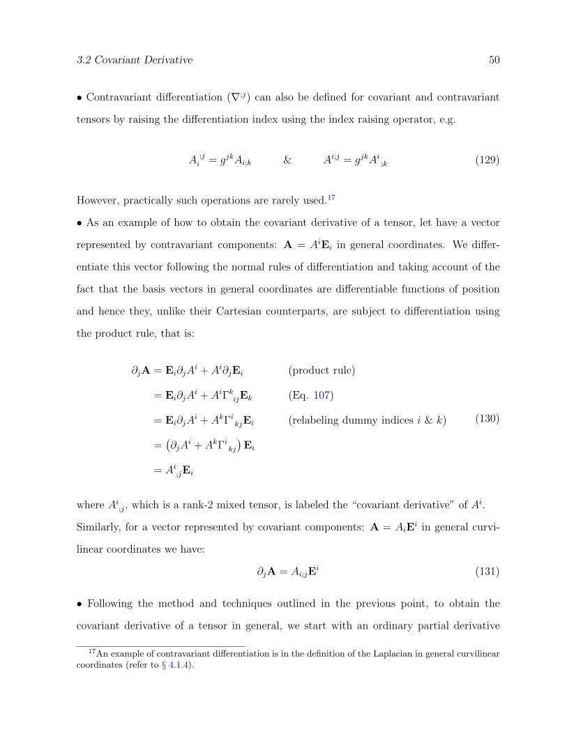
• As an example of how to obtain the covariant derivative of a tensor, let have a vector
represented by contravariant components: A = AiEi in general coordinates. We differ-
entiate this vector following the normal rules of differentiation and taking account of the
fact that the basis vectors in general coordinates are differentiable functions of position
and hence they, unlike their Cartesian counterparts, are subject to differentiation using
the product rule, that is:
∂jA = Ei∂jAi + Ai∂jEi (product rule)
= Ei∂jAi + AiΓkijEk (Eq. 107)
= Ei∂jAi + AkΓi kjEi (relabeling dummy indices i & k)
=(∂jA
i + AkΓi kj)Ei
= Ai;jEi
(130)
where Ai;j, which is a rank-2 mixed tensor, is labeled the “covariant derivative” of Ai.
Similarly, for a vector represented by covariant components: A = AiEi in general curvi-
linear coordinates we have:
∂jA = Ai;jEi (131)
• Following the method and techniques outlined in the previous point, to obtain the
covariant derivative of a tensor in general, we start with an ordinary partial derivative
17An example of contravariant differentiation is in the definition of the Laplacian in general curvilinearcoordinates (refer to § 4.1.4).
3.2 Covariant Derivative 51
term of the given tensor. Then for each tensor index an extra Christoffel symbol term
is added, positive for contravariant indices and negative for covariant indices, where the
differentiation index is one of the lower indices in the Christoffel symbol. Hence, for a
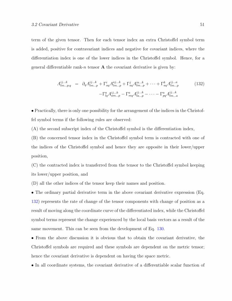
general differentiable rank-n tensor A the covariant derivative is given by:
Aij...klm...p;q = ∂qAij...klm...p + ΓiaqA
aj...klm...p + ΓjaqA
ia...klm...p + · · ·+ ΓkaqA
ij...alm...p (132)
−ΓalqAij...kam...p − ΓamqA
ij...kla...p − · · · − ΓapqA
ij...klm...a
• Practically, there is only one possibility for the arrangement of the indices in the Christof-
fel symbol terms if the following rules are observed:
(A) the second subscript index of the Christoffel symbol is the differentiation index,
(B) the concerned tensor index in the Christoffel symbol term is contracted with one of
the indices of the Christoffel symbol and hence they are opposite in their lower/upper
position,
(C) the contracted index is transferred from the tensor to the Christoffel symbol keeping
its lower/upper position, and
(D) all the other indices of the tensor keep their names and position.
• The ordinary partial derivative term in the above covariant derivative expression (Eq.
132) represents the rate of change of the tensor components with change of position as a
result of moving along the coordinate curve of the differentiated index, while the Christoffel
symbol terms represent the change experienced by the local basis vectors as a result of the
same movement. This can be seen from the development of Eq. 130.
• From the above discussion it is obvious that to obtain the covariant derivative, the
Christoffel symbols are required and these symbols are dependent on the metric tensor;
hence the covariant derivative is dependent on having the space metric.
• In all coordinate systems, the covariant derivative of a differentiable scalar function of
3.2 Covariant Derivative 52
position, f , is the same as the ordinary partial derivative, that is:
f;i = f,i = ∂if (133)
This is justified by the fact that the covariant derivative is different from the ordinary
partial derivative because the basis vectors in general coordinate systems are dependent
on their spatial position, and since a scalar is independent of the basis vectors the covari-
ant derivative and partial derivative are identical. This can also be concluded from the
covariant derivative rule as stated in the previous points and formulated in Eq. 132.
• Several rules of normal differentiation are naturally extended to covariant differentiation.
For example, covariant differentiation is a linear operation with respect to algebraic sums
of tensor terms and hence the covariant derivative of a sum is the sum of the covariant
derivatives of the terms:
(aA± bB);i = a (A);i ± b (B);i (134)
where a and b are scalar constants and A and B are differentiable tensors. The product
rule of ordinary differentiation also applies to covariant differentiation of inner and outer
products of tensors:
(A ◦B);i = (A);i ◦B + A ◦ (B);i (135)
where the symbol ◦ denotes an inner or outer product operator.
• According to the “Ricci Theorem”, the covariant derivative of the covariant and con-
travariant metric tensor is zero. This has nothing to do with the metric tensor being a
constant function of coordinates, which is true only for the rectilinear systems, but this
arises from the fact that the covariant derivative quantifies the change with position of the
basis vectors in magnitude and direction as well as the change in components, and these
3.2 Covariant Derivative 53
contributions in the case of the metric tensor cancel each other resulting in a total null
effect. As a result, the metric tensor behaves as a constant with respect to the covariant
derivative operation:
gij;k = 0 & gij;k = 0 (136)
for all values of the indices, and hence the covariant derivative operator bypasses the metric
tensor:
(g ◦A);k = g ◦ (A);k (137)
where A is a general tensor, g is the metric tensor in its covariant or contravariant form
and ◦ denotes an inner or outer tensor product.18
• As a result of the Ricci Theorem, the covariant derivative operator and the index shifting
operator are commutative, e.g.
(gikA
k)
;j= gikA
k;j = Ai;j = (Ai);j =
(gikA
k)
;j(138)
(gmignjAmn);k = gmignjA
mn;k = Aij;k = (Aij);k = (gmignjA
mn);k (139)
• Like the metric tensor, the Kronecker delta is constant with regard to the covariant
differentiation and hence the covariant derivative of the Kronecker delta is identically
zero:
δij;k = ∂kδij + δajΓ
iak − δiaΓajk = 0 + Γijk − Γijk = 0 (140)
The rule of the Kronecker delta may be regarded as an instance of the rule of the metric
tensor, as stated by the Ricci Theorem, since the Kronecker delta is a metric tensor.
Likewise, the covariant differentiation operator bypasses the Kronecker delta which is
18Although the metric tensor is normally used in inner product operations for raising and lowering ofindices, the possibility of its involvement in outer product operations should not be ruled out.
3.2 Covariant Derivative 54
involved in inner and outer tensor products:19
(δ ◦A);k = δ ◦ (A);k (141)
• Like the ordinary Kronecker delta, the covariant derivative of the generalized Kronecker
delta is identically zero.
• For a differentiable function f(x, y) of class C2 (i.e. all the second order partial derivatives
of the function do exist and are continuous), the mixed partial derivatives are equal, that
is:
∂x∂yf = ∂y∂xf (142)
However, even if the components of a tensor satisfy this condition (i.e. being of class C2),
this is not sufficient for the equality of the mixed covariant derivatives. What is required
for the mixed covariant derivatives to be equal is the vanishing of the Riemann Tensor
(see § 5.1).
• Higher order covariant derivatives are similarly defined as derivatives of derivatives
by successive repetition of the process of covariant differentiation; however the order of
differentiation should be respected as stated in the previous point. For example, the second
order mixed jk covariant derivative of a contravariant vector A is given by:
Ai;jk = ∂k∂jAi + Γika∂jA
a − Γajk∂aAi + Γija∂kA
a + Aa(∂jΓ
ika − ΓbjkΓ
iba + ΓijbΓ
bka
)(143)
while the second order mixed jk covariant derivative of a covariant vector A is given by:
Ai;jk = ∂k∂jAi − Γaij∂kAa − Γaik∂jAa − Γajk∂aAi − Aa(∂kΓ
aij − ΓaibΓ
bjk − ΓbikΓ
abj
)(144)
19Like the metric tensor, the Kronecker delta is normally used in inner product operations for replace-ment of indices; however the possibility of its involvement in outer product operations should not be ruledout.
3.2 Covariant Derivative 55
• The second order mixed kj covariant derivative of contravariant and covariant vectors
can be obtained from the equations in the last point by interchanging the j and k indices
and hence the inequality of the jk and kj mixed derivatives in general can be verified
(refer to § 5.1).
• The covariant derivative of a tensor is a tensor whose covariant rank is higher than the
covariant rank of the original tensor by one. Hence, the covariant derivative of a rank-n
tensor of type (r, s) is a rank-(n+ 1) tensor of type (r, s+ 1).
• Covariant differentiation and contraction of index operations commute with each other,
e.g. (Aijk)
;lδkj =
(Aijk δ
kj
);l
=(Aikk)
;l(145)
• Since the Christoffel symbols vanish when the components of the metric tensor in a
given coordinate system are constants, the covariant derivative is reduced to the ordinary
derivative in such systems. This is particularly true in Euclidean spaces coordinated by
rectilinear systems.
• The covariant derivatives of relative tensors, which are also relative tensors of the same
weight as the original tensors, are obtained by adding a weight term to the normal formulae
of covariant derivative. Hence, the covariant derivative of a relative scalar with weight w
is given by:
f;i = f,i − wfΓjji (146)
while the covariant derivative of relative tensors of higher ranks with weight w is obtained
by adding the following term to the right hand side of Eq. 132:
−wAij...klm...pΓaaq (147)
• Unlike ordinary differentiation, the covariant derivative of a non-scalar tensor with con-
stant components is not zero in general due to the presence of the Christoffel symbols in
3.3 Absolute Derivative 56
the definition of the covariant derivative, as given by Eq. 132.
• In rectilinear coordinates, the Christoffel symbols are identically zero because the basis
vectors are constants, and hence the covariant derivative is the same as the normal partial
derivative for all tensor ranks. As a result, when the components of the metric tensor, gij,
are constants as in the case of rectangular coordinate systems, the covariant derivative
becomes the ordinary partial derivative.
• For a differentiable covariant vector A which is a gradient of a scalar we have:
Ai;j = Aj;i (148)
• The covariant derivative of the basis vectors of the covariant and contravariant types is
identically zero:
Ei;j = ∂jEi − ΓkijEk = ΓkijEk − ΓkijEk = 0
Ei;j = ∂jE
i + ΓikjEk = −ΓikjE
k + ΓikjEk = 0
(149)
3.3 Absolute Derivative
• The absolute derivative of a tensor along a t-parameterized curve in an nD space with
respect to the parameter t is the inner product of the covariant derivative of the tensor and
the tangent vector to the curve. In brief, the absolute derivative is a covariant derivative
of a tensor along a curve.
• For a tensor Ai, the inner product of Ai;j, which is a tensor, with another tensor is a
tensor. Now, if the other tensor is dui
dt, which is the tangent vector to a t-parameterized
curve L given by the equations ui = ui(t), then the inner product:
Ai;rdur
dt(150)
is a tensor of the same rank and type as the tensor Ai. The tensor given by the expression
3.3 Absolute Derivative 57
150 is called the “absolute” or “intrinsic” or “absolute covariant” derivative of the tensor
Ai along the curve L and is symbolized by:
δAi
δt(151)
• For a differentiable scalar f , the absolute derivative, like the covariant derivative, is the
same as the ordinary derivative, that is:
δf
δt=df
dt(152)
• The absolute derivative of a differentiable contravariant vector Ak with respect to the
parameter t is given by:
δAk
δt=dAk
dt+ ΓkijA
iduj
dt(153)
Similarly for a differentiable covariant vector Ak we have:
δAkδt
=dAkdt− ΓikjAi
duj
dt(154)
• Absolute differentiation can be easily extended to higher rank (> 1) differentiable tensors
of type (m,n) along parameterized curves. For instance, the absolute derivative of a mixed
tensor of type (1, 2) Aijk along a t-parameterized curve L is given by:
δAijkδt
= Aijk;b
dub
dt=dAijkdt
+ ΓiabAajk
dub
dt− ΓajbA
iak
dub
dt− ΓabkA
ija
dub
dt(155)
• As the absolute derivative is given generically by:
δA
δt= (A);k
duk
dt(156)
3.3 Absolute Derivative 58
it can be seen as an instance of the chain rule of differentiation where the two contracted
indices represent the in-between coordinate differential.
• Because the absolute derivative along a curve is just an inner product of the covariant
derivative with the vector tangent to the curve, the well known rules of ordinary dif-
ferentiation of sums and products also apply to absolute differentiation, as for covariant
differentiation, that is:
δ
δt(aA + bB) = a
δA
δt+ b
δB
δt(157)
δ
δt(A ◦B) =
(δA
δt◦B
)+
(A ◦ δB
δt
)(158)
where a and b are constant scalars, A and B are differentiable tensors and the symbol ◦
denotes an inner or outer product of tensors.
• The covariant and contravariant metric tensors are in lieu of constants with respect to
absolute differentiation, that is:
δgijδt
= 0 &δgij
δt= 0 (159)
and hence they pass through the absolute derivative operator:
δ (gijAj)
δt= gij
δAj
δt&
δ (gijAj)
δt= gij
δAjδt
(160)
• For coordinate systems in which all the components of the metric tensor are constants,
the absolute derivative is the same as the ordinary derivative. This is the case in the
rectilinear coordinate systems.
• The absolute derivative of a tensor along a given curve is unique, and hence the ordinary
derivative of the tensor along that curve in a rectangular coordinate system is the same
as the absolute derivative of the tensor along that curve in any other system.
4 DIFFERENTIAL OPERATIONS 59
4 Differential Operations
• In this section we generalize and expand what have been given in the previous notes
[11] about the main differential operations which are based on the nabla operator ∇. The
section will investigate these operations in general curvilinear coordinate systems and in
general orthogonal coordinate systems which are a special case of the general curvilinear
systems. We also investigate the two most important and widely used non-Cartesian
orthogonal coordinate systems, namely the cylindrical and spherical systems, due to their
particular importance.
4.1 General Curvilinear Coordinate System
• Here, we investigate the differential operations and operators in general curvilinear
coordinate systems, whether orthogonal or not.
• The previous definitions of the differential operations, as given in the first set of notes,
are essentially valid in general non-Cartesian coordinate systems if the operations are
extended to include the basis vectors as well as the components.
• The analytical expressions of the differential operations can be obtained directly if the
expression for the nabla operator ∇ and the spatial derivatives of the basis vectors in the
general curvilinear coordinate system are known.
4.1.1 Gradient
• The nabla operator ∇ in general curvilinear coordinate systems is defined as follow:
∇ = Ei∂i (161)
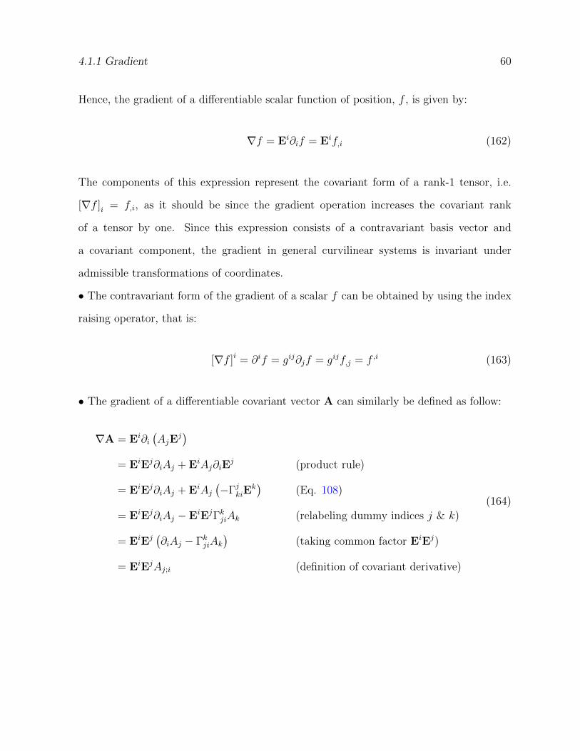
4.1.1 Gradient 60
Hence, the gradient of a differentiable scalar function of position, f , is given by:
∇f = Ei∂if = Eif,i (162)
The components of this expression represent the covariant form of a rank-1 tensor, i.e.
[∇f ]i = f,i, as it should be since the gradient operation increases the covariant rank
of a tensor by one. Since this expression consists of a contravariant basis vector and
a covariant component, the gradient in general curvilinear systems is invariant under
admissible transformations of coordinates.
• The contravariant form of the gradient of a scalar f can be obtained by using the index
raising operator, that is:
[∇f ]i = ∂if = gij∂jf = gijf,j = f ,i (163)
• The gradient of a differentiable covariant vector A can similarly be defined as follow:
∇A = Ei∂i(AjE
j)
= EiEj∂iAj + EiAj∂iEj (product rule)
= EiEj∂iAj + EiAj(−ΓjkiE
k)
(Eq. 108)
= EiEj∂iAj − EiEjΓkjiAk (relabeling dummy indices j & k)
= EiEj(∂iAj − ΓkjiAk
)(taking common factor EiEj)
= EiEjAj;i (definition of covariant derivative)
(164)
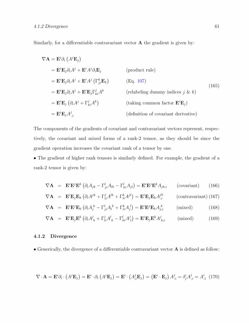
4.1.2 Divergence 61
Similarly, for a differentiable contravariant vector A the gradient is given by:
∇A = Ei∂i(AjEj
)= EiEj∂iA
j + EiAj∂iEj (product rule)
= EiEj∂iAj + EiAj
(ΓkjiEk
)(Eq. 107)
= EiEj∂iAj + EiEjΓ
jkiA
k (relabeling dummy indices j & k)
= EiEj
(∂iA
j + ΓjkiAk)
(taking common factor EiEj)
= EiEjAj;i (definition of covariant derivative)
(165)
The components of the gradients of covariant and contravariant vectors represent, respec-
tively, the covariant and mixed forms of a rank-2 tensor, as they should be since the
gradient operation increases the covariant rank of a tensor by one.
• The gradient of higher rank tensors is similarly defined. For example, the gradient of a
rank-2 tensor is given by:
∇A = EiEjEk(∂iAjk − ΓljiAlk − ΓlkiAjl
)= EiEjEkAjk;i (covariant) (166)
∇A = EiEjEk
(∂iA
jk + ΓjliAlk + ΓkliA
jl)
= EiEjEkAjk;i (contravariant) (167)
∇A = EiEjEk
(∂iA
kj − ΓljiA
kl + ΓkliA
lj
)= EiEjEkA
kj;i (mixed) (168)
∇A = EiEjEk(∂iA
jk + ΓjliA
lk − ΓlkiA
jl
)= EiEjE
kAjk;i (mixed) (169)
4.1.2 Divergence
• Generically, the divergence of a differentiable contravariant vector A is defined as follow:
∇·A = Ei∂i ·(AjEj
)= Ei ·∂i
(AjEj
)= Ei ·
(Aj;iEj
)=(Ei · Ej
)Aj;i = δijA
j;i = Ai;i (170)
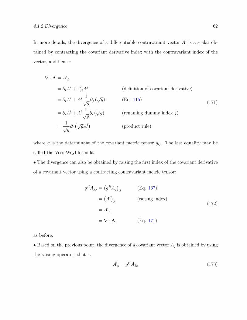
4.1.2 Divergence 62
In more details, the divergence of a differentiable contravariant vector Ai is a scalar ob-
tained by contracting the covariant derivative index with the contravariant index of the
vector, and hence:
∇ ·A = Ai;i
= ∂iAi + ΓijiA
j (definition of covariant derivative)
= ∂iAi + Aj
1√g∂j (√g) (Eq. 115)
= ∂iAi + Ai
1√g∂i (√g) (renaming dummy index j)
=1√g∂i(√
gAi)
(product rule)
(171)
where g is the determinant of the covariant metric tensor gij. The last equality may be
called the Voss-Weyl formula.
• The divergence can also be obtained by raising the first index of the covariant derivative
of a covariant vector using a contracting contravariant metric tensor:
gjiAj;i =(gjiAj
);i
(Eq. 137)
=(Ai)
;i(raising index)
= Ai;i
= ∇ ·A (Eq. 171)
(172)
as before.
• Based on the previous point, the divergence of a covariant vector Aj is obtained by using
the raising operator, that is
Ai;i = gijAj;i (173)
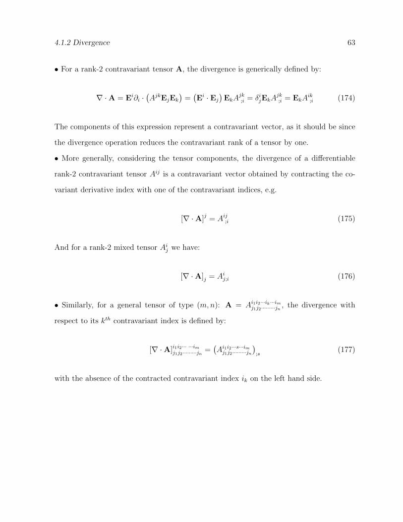
4.1.2 Divergence 63
• For a rank-2 contravariant tensor A, the divergence is generically defined by:
∇ ·A = Ei∂i ·(AjkEjEk
)=(Ei · Ej
)EkA
jk;i = δijEkA
jk;i = EkA
ik;i (174)
The components of this expression represent a contravariant vector, as it should be since
the divergence operation reduces the contravariant rank of a tensor by one.
• More generally, considering the tensor components, the divergence of a differentiable
rank-2 contravariant tensor Aij is a contravariant vector obtained by contracting the co-
variant derivative index with one of the contravariant indices, e.g.
[∇ ·A]j = Aij;i (175)
And for a rank-2 mixed tensor Aij we have:
[∇ ·A]j = Aij;i (176)
• Similarly, for a general tensor of type (m,n): A = Ai1i2···ik···imj1j2·········jn , the divergence with
respect to its kth contravariant index is defined by:
[∇ ·A]i1i2··· ···imj1j2·········jn =(Ai1i2···s···imj1j2·········jn
);s
(177)
with the absence of the contracted contravariant index ik on the left hand side.
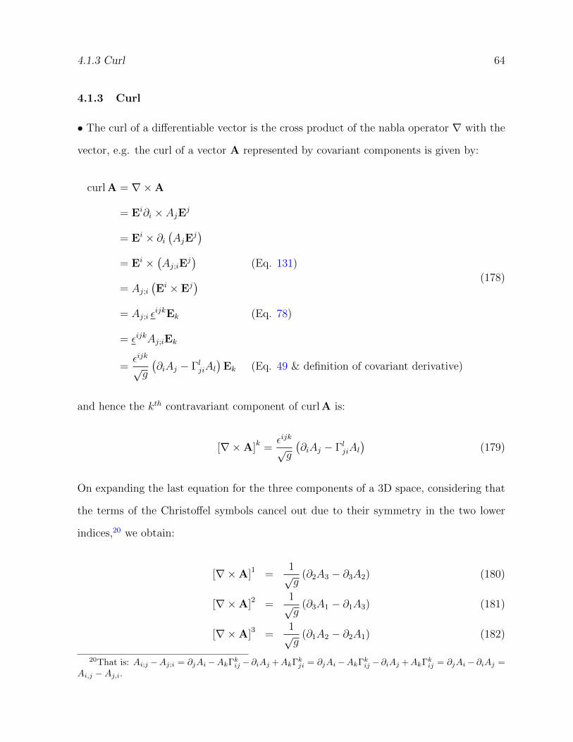
4.1.3 Curl 64
4.1.3 Curl
• The curl of a differentiable vector is the cross product of the nabla operator ∇ with the
vector, e.g. the curl of a vector A represented by covariant components is given by:
curl A = ∇×A
= Ei∂i × AjEj
= Ei × ∂i(AjE
j)
= Ei ×(Aj;iE
j)
(Eq. 131)
= Aj;i(Ei × Ej
)= Aj;i ε
ijkEk (Eq. 78)
= εijkAj;iEk
=εijk√g
(∂iAj − ΓljiAl
)Ek (Eq. 49 & definition of covariant derivative)
(178)
and hence the kth contravariant component of curl A is:
[∇×A]k =εijk√g
(∂iAj − ΓljiAl
)(179)
On expanding the last equation for the three components of a 3D space, considering that
the terms of the Christoffel symbols cancel out due to their symmetry in the two lower
indices,20 we obtain:
[∇×A]1 =1√g
(∂2A3 − ∂3A2) (180)
[∇×A]2 =1√g
(∂3A1 − ∂1A3) (181)
[∇×A]3 =1√g
(∂1A2 − ∂2A1) (182)
20That is: Ai;j −Aj;i = ∂jAi−AkΓkij − ∂iAj +AkΓkji = ∂jAi−AkΓkij − ∂iAj +AkΓkij = ∂jAi− ∂iAj =Ai,j −Aj,i.
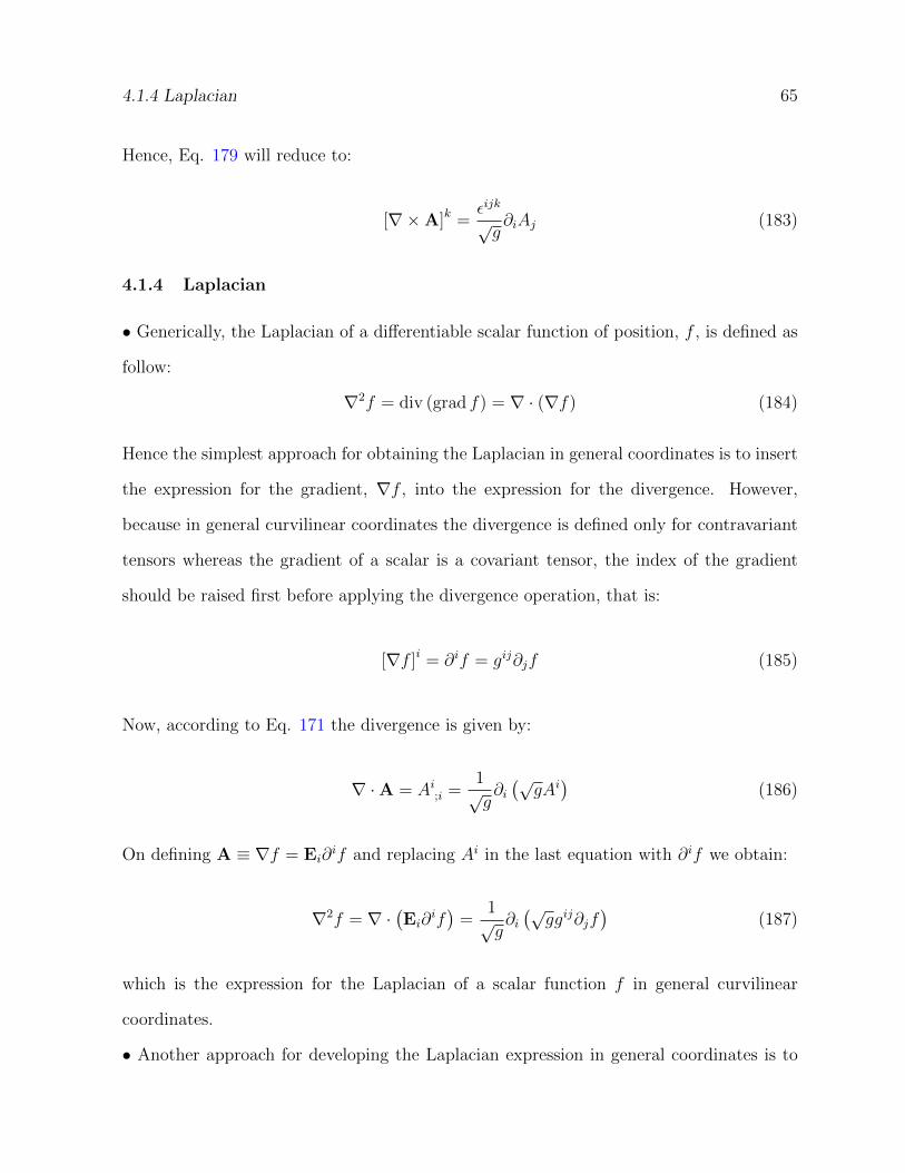
4.1.4 Laplacian 65
Hence, Eq. 179 will reduce to:
[∇×A]k =εijk√g∂iAj (183)
4.1.4 Laplacian
• Generically, the Laplacian of a differentiable scalar function of position, f , is defined as
follow:
∇2f = div (grad f) = ∇ · (∇f) (184)
Hence the simplest approach for obtaining the Laplacian in general coordinates is to insert
the expression for the gradient, ∇f , into the expression for the divergence. However,
because in general curvilinear coordinates the divergence is defined only for contravariant
tensors whereas the gradient of a scalar is a covariant tensor, the index of the gradient
should be raised first before applying the divergence operation, that is:
[∇f ]i = ∂if = gij∂jf (185)
Now, according to Eq. 171 the divergence is given by:
∇ ·A = Ai;i =1√g∂i(√
gAi)
(186)
On defining A ≡ ∇f = Ei∂if and replacing Ai in the last equation with ∂if we obtain:
∇2f = ∇ ·(Ei∂
if)
=1√g∂i(√
ggij∂jf)
(187)
which is the expression for the Laplacian of a scalar function f in general curvilinear
coordinates.
• Another approach for developing the Laplacian expression in general coordinates is to
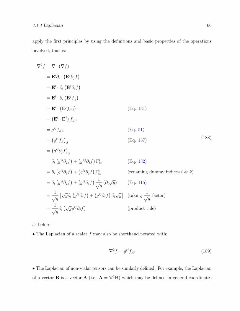
4.1.4 Laplacian 66
apply the first principles by using the definitions and basic properties of the operations
involved, that is:
∇2f = ∇ · (∇f)
= Ei∂i ·(Ej∂jf
)= Ei · ∂i
(Ej∂jf
)= Ei · ∂i
(Ejf,j
)= Ei ·
(Ejf,j;i
)(Eq. 131)
=(Ei · Ej
)f,j;i
= gijf,j;i (Eq. 51)
=(gijf,j
);i
(Eq. 137)
=(gij∂jf
);i
= ∂i(gij∂jf
)+(gkj∂jf
)Γiki (Eq. 132)
= ∂i(gij∂jf
)+(gij∂jf
)Γkik (renaming dummy indices i & k)
= ∂i(gij∂jf
)+(gij∂jf
) 1√g
(∂i√g) (Eq. 115)
=1√g
[√g∂i(gij∂jf
)+(gij∂jf
)∂i√g]
(taking1√g
factor)
=1√g∂i(√
ggij∂jf)
(product rule)
(188)
as before.
• The Laplacian of a scalar f may also be shorthand notated with:
∇2f = gijf,ij (189)
• The Laplacian of non-scalar tensors can be similarly defined. For example, the Laplacian
of a vector B is a vector A (i.e. A = ∇2B) which may be defined in general coordinates
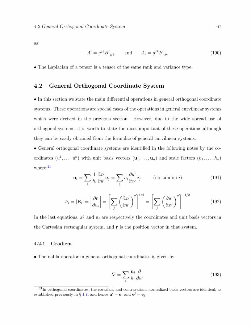
4.2 General Orthogonal Coordinate System 67
as:
Ai = gjkBi;jk and Ai = gjkBi;jk (190)
• The Laplacian of a tensor is a tensor of the same rank and variance type.
4.2 General Orthogonal Coordinate System
• In this section we state the main differential operations in general orthogonal coordinate
systems. These operations are special cases of the operations in general curvilinear systems
which were derived in the previous section. However, due to the wide spread use of
orthogonal systems, it is worth to state the most important of these operations although
they can be easily obtained from the formulae of general curvilinear systems.
• General orthogonal coordinate systems are identified in the following notes by the co-
ordinates (u1, . . . , un) with unit basis vectors (u1, . . . ,un) and scale factors (h1, . . . , hn)
where:21
ui =∑j
1
hi
∂xj
∂uiej =
∑j
hi∂ui
∂xjej (no sum on i) (191)
hi = |Ei| =∣∣∣∣ ∂r
∂ui
∣∣∣∣ =
[∑j
(∂xj
∂ui
)2]1/2
=
[∑j
(∂ui
∂xj
)2]−1/2
(192)
In the last equations, xj and ej are respectively the coordinates and unit basis vectors in
the Cartesian rectangular system, and r is the position vector in that system.
4.2.1 Gradient
• The nabla operator in general orthogonal coordinates is given by:
∇ =∑i
uihi
∂
∂ui(193)
21In orthogonal coordinates, the covariant and contravariant normalized basis vectors are identical, asestablished previously in § 1.7, and hence ui = ui and ej = ej .
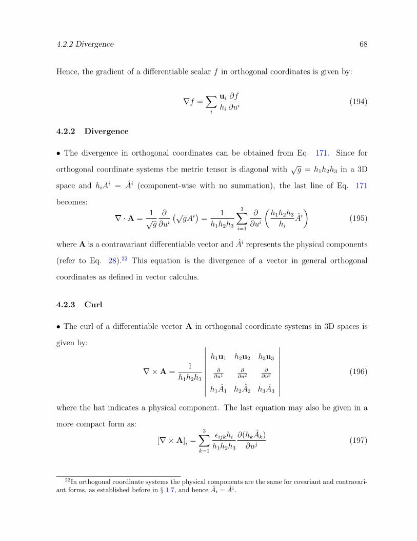
4.2.2 Divergence 68
Hence, the gradient of a differentiable scalar f in orthogonal coordinates is given by:
∇f =∑i
uihi
∂f
∂ui(194)
4.2.2 Divergence
• The divergence in orthogonal coordinates can be obtained from Eq. 171. Since for
orthogonal coordinate systems the metric tensor is diagonal with√g = h1h2h3 in a 3D
space and hiAi = Ai (component-wise with no summation), the last line of Eq. 171
becomes:
∇ ·A =1√g
∂
∂ui(√
gAi)
=1
h1h2h3
3∑i=1
∂
∂ui
(h1h2h3
hiAi)
(195)
where A is a contravariant differentiable vector and Ai represents the physical components
(refer to Eq. 28).22 This equation is the divergence of a vector in general orthogonal
coordinates as defined in vector calculus.
4.2.3 Curl
• The curl of a differentiable vector A in orthogonal coordinate systems in 3D spaces is
given by:
∇×A =1
h1h2h3
∣∣∣∣∣∣∣∣∣∣h1u1 h2u2 h3u3
∂∂u1
∂∂u2
∂∂u3
h1A1 h2A2 h3A3
∣∣∣∣∣∣∣∣∣∣(196)
where the hat indicates a physical component. The last equation may also be given in a
more compact form as:
[∇×A]i =3∑
k=1
εijkhih1h2h3
∂(hkAk)
∂uj(197)
22In orthogonal coordinate systems the physical components are the same for covariant and contravari-ant forms, as established before in § 1.7, and hence Ai = Ai.
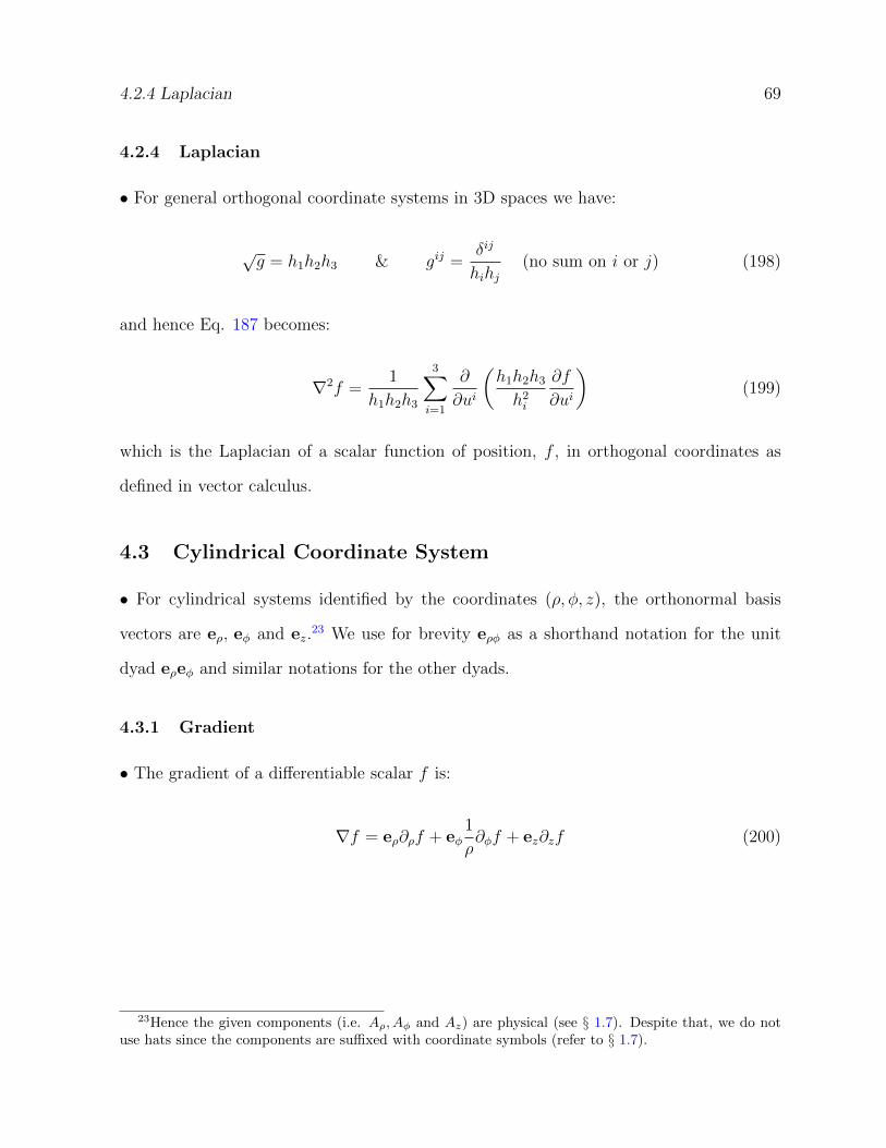
4.2.4 Laplacian 69
4.2.4 Laplacian
• For general orthogonal coordinate systems in 3D spaces we have:
√g = h1h2h3 & gij =
δij
hihj(no sum on i or j) (198)
and hence Eq. 187 becomes:
∇2f =1
h1h2h3
3∑i=1
∂
∂ui
(h1h2h3
h2i
∂f
∂ui
)(199)
which is the Laplacian of a scalar function of position, f , in orthogonal coordinates as
defined in vector calculus.
4.3 Cylindrical Coordinate System
• For cylindrical systems identified by the coordinates (ρ, φ, z), the orthonormal basis
vectors are eρ, eφ and ez.23 We use for brevity eρφ as a shorthand notation for the unit
dyad eρeφ and similar notations for the other dyads.
4.3.1 Gradient
• The gradient of a differentiable scalar f is:
∇f = eρ∂ρf + eφ1
ρ∂φf + ez∂zf (200)
23Hence the given components (i.e. Aρ, Aφ and Az) are physical (see § 1.7). Despite that, we do notuse hats since the components are suffixed with coordinate symbols (refer to § 1.7).
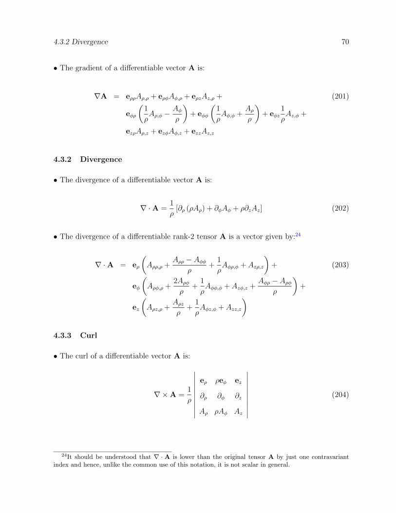
4.3.2 Divergence 70
• The gradient of a differentiable vector A is:
∇A = eρρAρ,ρ + eρφAφ,ρ + eρzAz,ρ + (201)
eφρ
(1
ρAρ,φ −
Aφρ
)+ eφφ
(1
ρAφ,φ +
Aρρ
)+ eφz
1
ρAz,φ +
ezρAρ,z + ezφAφ,z + ezzAz,z
4.3.2 Divergence
• The divergence of a differentiable vector A is:
∇ ·A =1
ρ[∂ρ (ρAρ) + ∂φAφ + ρ∂zAz] (202)
• The divergence of a differentiable rank-2 tensor A is a vector given by:24
∇ ·A = eρ
(Aρρ,ρ +
Aρρ − Aφφρ
+1
ρAφρ,φ + Azρ,z
)+ (203)
eφ
(Aρφ,ρ +
2Aρφρ
+1
ρAφφ,φ + Azφ,z +
Aφρ − Aρφρ
)+
ez
(Aρz,ρ +
Aρzρ
+1
ρAφz,φ + Azz,z
)
4.3.3 Curl
• The curl of a differentiable vector A is:
∇×A =1
ρ
∣∣∣∣∣∣∣∣∣∣eρ ρeφ ez
∂ρ ∂φ ∂z
Aρ ρAφ Az
∣∣∣∣∣∣∣∣∣∣(204)
24It should be understood that ∇ · A is lower than the original tensor A by just one contravariantindex and hence, unlike the common use of this notation, it is not scalar in general.
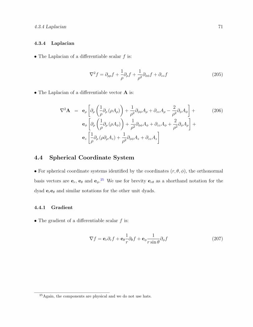
4.3.4 Laplacian 71
4.3.4 Laplacian
• The Laplacian of a differentiable scalar f is:
∇2f = ∂ρρf +1
ρ∂ρf +
1
ρ2∂φφf + ∂zzf (205)
• The Laplacian of a differentiable vector A is:
∇2A = eρ
[∂ρ
(1
ρ∂ρ (ρAρ)
)+
1
ρ2∂φφAρ + ∂zzAρ −
2
ρ2∂φAφ
]+ (206)
eφ
[∂ρ
(1
ρ∂ρ (ρAφ)
)+
1
ρ2∂φφAφ + ∂zzAφ +
2
ρ2∂φAρ
]+
ez
[1
ρ∂ρ (ρ∂ρAz) +
1
ρ2∂φφAz + ∂zzAz
]
4.4 Spherical Coordinate System
• For spherical coordinate systems identified by the coordinates (r, θ, φ), the orthonormal
basis vectors are er, eθ and eφ.25 We use for brevity erθ as a shorthand notation for the
dyad ereθ and similar notations for the other unit dyads.
4.4.1 Gradient
• The gradient of a differentiable scalar f is:
∇f = er∂rf + eθ1
r∂θf + eφ
1
r sin θ∂φf (207)
25Again, the components are physical and we do not use hats.
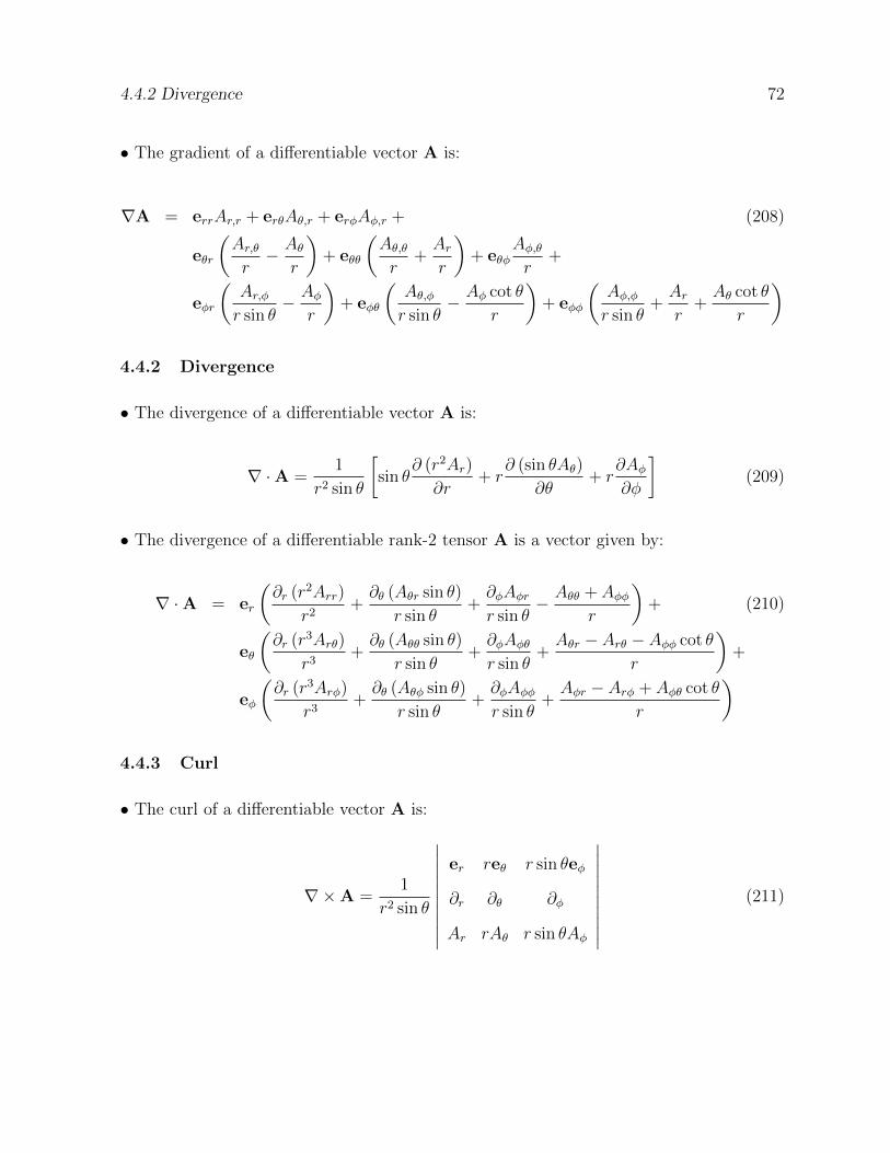
4.4.2 Divergence 72
• The gradient of a differentiable vector A is:
∇A = errAr,r + erθAθ,r + erφAφ,r + (208)
eθr
(Ar,θr− Aθ
r
)+ eθθ
(Aθ,θr
+Arr
)+ eθφ
Aφ,θr
+
eφr
(Ar,φr sin θ
− Aφr
)+ eφθ
(Aθ,φr sin θ
− Aφ cot θ
r
)+ eφφ
(Aφ,φr sin θ
+Arr
+Aθ cot θ
r
)
4.4.2 Divergence
• The divergence of a differentiable vector A is:
∇ ·A =1
r2 sin θ
[sin θ
∂ (r2Ar)
∂r+ r
∂ (sin θAθ)
∂θ+ r
∂Aφ∂φ
](209)
• The divergence of a differentiable rank-2 tensor A is a vector given by:
∇ ·A = er
(∂r (r2Arr)
r2+∂θ (Aθr sin θ)
r sin θ+∂φAφrr sin θ
− Aθθ + Aφφr
)+ (210)
eθ
(∂r (r3Arθ)
r3+∂θ (Aθθ sin θ)
r sin θ+∂φAφθr sin θ
+Aθr − Arθ − Aφφ cot θ
r
)+
eφ
(∂r (r3Arφ)
r3+∂θ (Aθφ sin θ)
r sin θ+∂φAφφr sin θ
+Aφr − Arφ + Aφθ cot θ
r
)
4.4.3 Curl
• The curl of a differentiable vector A is:
∇×A =1
r2 sin θ
∣∣∣∣∣∣∣∣∣∣er reθ r sin θeφ
∂r ∂θ ∂φ
Ar rAθ r sin θAφ
∣∣∣∣∣∣∣∣∣∣(211)
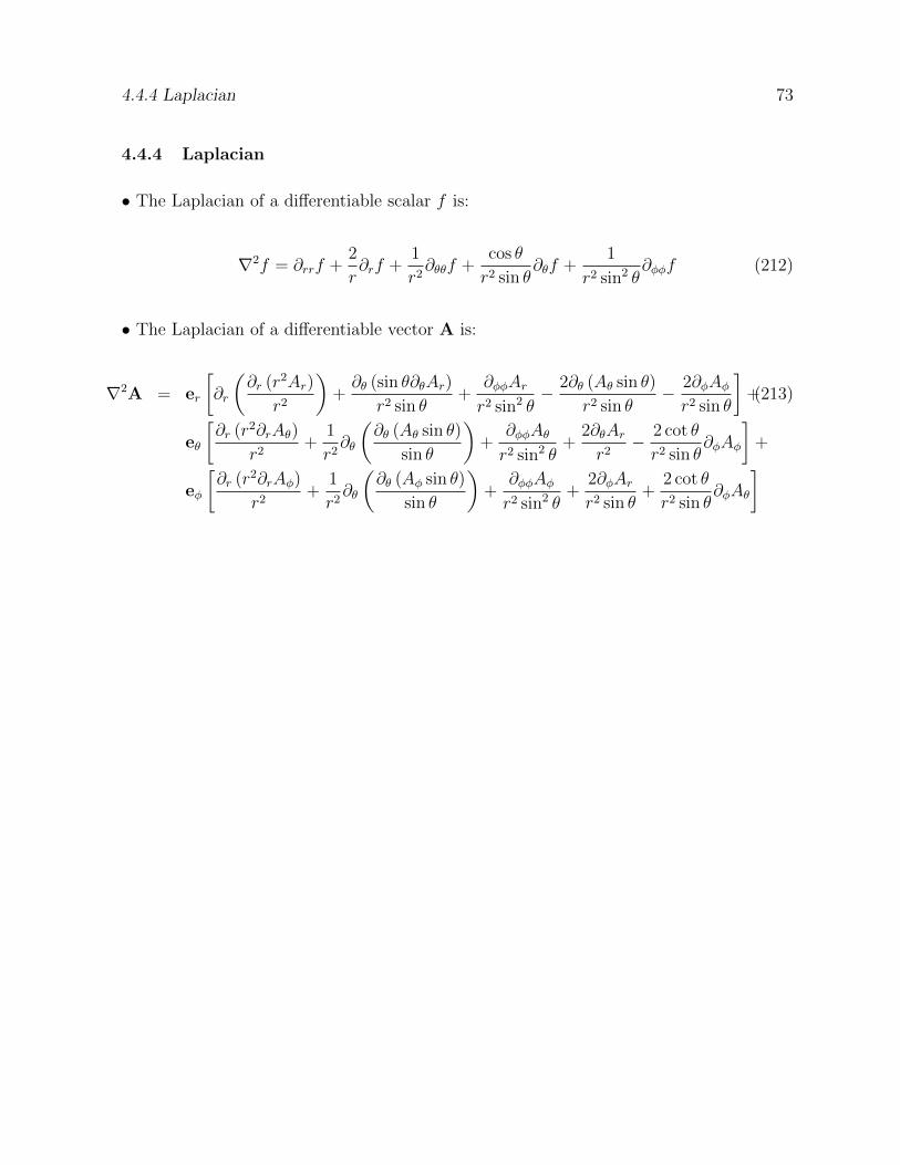
4.4.4 Laplacian 73
4.4.4 Laplacian
• The Laplacian of a differentiable scalar f is:
∇2f = ∂rrf +2
r∂rf +
1
r2∂θθf +
cos θ
r2 sin θ∂θf +
1
r2 sin2 θ∂φφf (212)
• The Laplacian of a differentiable vector A is:
∇2A = er
[∂r
(∂r (r2Ar)
r2
)+∂θ (sin θ∂θAr)
r2 sin θ+
∂φφArr2 sin2 θ
− 2∂θ (Aθ sin θ)
r2 sin θ− 2∂φAφr2 sin θ
]+(213)
eθ
[∂r (r2∂rAθ)
r2+
1
r2∂θ
(∂θ (Aθ sin θ)
sin θ
)+
∂φφAθr2 sin2 θ
+2∂θArr2
− 2 cot θ
r2 sin θ∂φAφ
]+
eφ
[∂r (r2∂rAφ)
r2+
1
r2∂θ
(∂θ (Aφ sin θ)
sin θ
)+
∂φφAφr2 sin2 θ
+2∂φArr2 sin θ
+2 cot θ
r2 sin θ∂φAθ
]
5 TENSORS IN APPLICATIONS 74
5 Tensors in Applications
• In this section we conduct a preliminary investigation of some commonly-used tensors in
physical and mathematical applications of tensor calculus in anticipation of the forthcom-
ing set of notes. Most of these tensors come from differential geometry, fluid, continuum
and relativistic mechanics, since these disciplines are intimately linked to tensor calculus as
large parts of the subject were developed, and are still developing, within these disciplines.
These tensors also form the building blocks of several physical and mathematical theories.
We would like to insist that these are just a few partially representative examples for the
use of tensors in scientific and mathematical applications to have more familiarity with
tensor language and techniques and hence they are not meant to provide a comprehensive
view in any way. We should also indicate that some tensors are defined differently in
different disciplines and hence the given definitions and properties may not be thorough
or general.
5.1 Riemann Tensor
• This rank-4 tensor, which is also called Riemann curvature tensor and Riemann-Christoffel
tensor, is a property of the space. It characterizes important properties of spaces and sur-
faces and hence it plays an important role in geometry in general and in non-Euclidean
geometries in particular.
• The covariant differentiation operators in mixed derivatives are not commutative and
hence for a covariant vector A we have:
Aj;kl − Aj;lk = RijklAi (214)
5.1 Riemann Tensor 75
where Rijkl is the Riemann tensor of the second kind which is given by:
Rijkl = ∂kΓ
ijl − ∂lΓijk + ΓrjlΓ
irk − ΓrjkΓ
irl (215)
• The last equation can be put into the following mnemonic determinantal form:
Rijkl =
∣∣∣∣∣∣∣∂k ∂l
Γijk Γijl
∣∣∣∣∣∣∣+
∣∣∣∣∣∣∣Γrjl Γrjk
Γirl Γirk
∣∣∣∣∣∣∣ (216)
• The Riemann-Christoffel tensor of the second kind is also called the mixed Riemann-
Christoffel tensor.
• From Eq. 214, it is obvious that the mixed second order covariant derivatives are equal
iff the Riemann tensor of the second kind vanishes identically.
• On lowering the contravariant index of the Riemann tensor of the second kind, the
Riemann tensor of the first kind is obtained:
Rijkl = giaRajkl (217)
• Alternatively, the Riemann tensor of the first kind can be established independently as:
Rijkl = ∂k [jl, i]− ∂l [jk, i] + [il, r] Γrjk − [ik, r] Γrjl
=1
2(∂j∂kgil + ∂i∂lgjk − ∂j∂lgik − ∂i∂kgjl) + [il, r] Γrjk − [ik, r] Γrjl (218)
=1
2(∂j∂kgil + ∂i∂lgjk − ∂j∂lgik − ∂i∂kgjl) + grs ([il, r] [jk, s]− [ik, r] [jl, s])
• The first line of the last equation can be cast in the following mnemonic determinantal
form:
Rijkl =
∣∣∣∣∣∣∣∂k ∂l
[jk, i] [jl, i]
∣∣∣∣∣∣∣+
∣∣∣∣∣∣∣Γrjk Γrjl
[ik, r] [il, r]
∣∣∣∣∣∣∣ (219)
5.1 Riemann Tensor 76
• Similarly, the Riemann-Christoffel tensor of the second kind can be obtained by raising
the first covariant index of the Riemann-Christoffel tensor of the first kind:
Rijkl = giaRajkl (220)
• The Riemann-Christoffel tensor of the first kind is also called the covariant (or totally
covariant) Riemann-Christoffel tensor.
• The covariant differentiation operators become commutative when the metric makes the
Riemann tensor of either kind vanish.
• For the mixed second order covariant derivatives of a contravariant vector A we have:
Aj;kl − Aj;lk = Rj
ilkAi (221)
which is similar to Eq. 214 for a covariant vector A.
• The Riemann-Christoffel tensor vanishes identically iff the space is globally flat. Hence,
the Riemann tensor is zero in Euclidean spaces, and consequently the mixed second order
covariant derivatives, which become ordinary derivatives, are equal when the C2 continuity
condition is satisfied.
• The Riemann curvature tensor depends only on the metric which, in general curvilinear
coordinates, is a function of position and hence the Riemann tensor follows this dependency
on position. Yes, for affine coordinates the metric tensor is constant and hence the Riemann
tensor vanishes identically.
• The totally covariant Riemann tensor satisfies the following symmetric and skew-symmetric
5.1 Riemann Tensor 77
relations in its four indices:
Rijkl = Rklij (block symmetry)
= −Rjikl (anti-symmetry in the first two indices) (222)
= −Rijlk (anti-symmetry in the last two indices)
• The skew-symmetric property of the covariant Riemann tensor with respect to the last
two indices also applies to the mixed Riemann tensor:
Rijkl = −Ri
jlk (223)
• As a consequence of the first and second anti-symmetric properties of the covariant
Riemann tensor, the entries of the Riemann tensor with identical values of the first two
indices or/and the last two indices are zero.
• As a consequence of the skew-symmetric properties of the Riemann tensor, all entries of
the tensor with identical values of more than two indices (e.g. Riiji) are zero.
• In an nD space, the Riemann tensor has n4 components.
• As a consequence of the symmetric and anti-symmetric properties of the Riemann tensor,
in an nD space there are three types of distinct non-vanishing entries:
A. Entries with only two distinct indices (type Rijij) which count:
N1 =n (n− 1)
2(224)
B. Entries with only three distinct indices (type Rijik) which count:
N2 =n (n− 1) (n− 2)
2(225)
5.1 Riemann Tensor 78
C. Entries with four distinct indices (type Rijkl) which count:
N3 =n (n− 1) (n− 2) (n− 3)
12(226)
• By adding the numbers of the three types of non-zero distinct entries, as given in the
last point, it can be shown that the Riemann tensor in an nD space has a total of
NRI = N1 +N2 +N3 =n2 (n2 − 1)
12(227)
independent components which do not vanish identically. For example, in a 2D Rie-
mannian space the Riemann tensor has 24 = 16 components; however there is only one
independent component (with the principal suffix 1212) which is not identically zero rep-
resented by the following four dependent components:
R1212 = R2121 = −R1221 = −R2112 (228)
Similarly, in a 3D Riemannian space the Riemann tensor has 34 = 81 components but only
six of these are distinct non-zero entries which are the ones with the following principal
suffixes:
1212, 1313, 1213, 2123, 3132, 2323 (229)
where the permutations of indices in each of these suffixes are subject to the symmetric
and anti-symmetric properties of the four indices of the Riemann tensor, as in the case of a
2D space in the above example, and hence these permutations do not produce independent
entries.
• Following the pattern in the last point, in a 4D Riemannian space the Riemann tensor
has 44 = 256 components but only 20 of these are independent non-zero entries, while in
a 5D Riemannian space the Riemann tensor has 54 = 625 components but only 50 are
5.1 Riemann Tensor 79
independent non-zero entries.
• The Riemann tensor satisfies the following identity:
Rijkl;s +Riljk;s = Riksl;j +Rikjs;l (230)
• A necessary and sufficient condition that a manifold for which there is a coordinate
system with all the components of the metric tensor being constants26 is that:
Rijkl = 0 (231)
• On contracting the first covariant index with the contravariant index of the Riemann
tensor of the second kind we obtain:
Riikl = ∂kΓ
iil − ∂lΓiik + ΓrilΓ
irk − ΓrikΓ
irl (j = i in Eq. 215)
= ∂kΓiil − ∂lΓiik + ΓrilΓ
irk − ΓirkΓ
ril (relabeling dummy i, r in last term)
= ∂kΓiil − ∂lΓiik
= ∂k [∂l (ln√g)]− ∂l [∂k (ln
√g)] (Eq. 115)
= ∂k∂l (ln√g)− ∂l∂k (ln
√g)
= ∂k∂l (ln√g)− ∂k∂l (ln
√g) (C2 condition is assumed)
= 0
(232)
That is:
Riikl = 0 (233)
26This may be called flat pseudo Riemannian manifold.
5.1.1 Bianchi identities 80
5.1.1 Bianchi identities
• The Riemann tensor of the first and second kind satisfies a number of identities called
the Bianchi identities.
• The first Bianchi identity is:
Rijkl +Riljk +Riklj = 0 (first kind)
Rijkl +Ri
ljk +Riklj = 0 (second kind)
(234)
These two forms of the first identity can be obtained from each other by the raising and
lowering operators.
• The above first Bianchi identity is an instance of the fact that by fixing the position of
one of the four indices and permuting the other three indices cyclically, the algebraic sum
of these three permuting forms is zero, that is:
Rijkl +Riljk +Riklj = 0 (i fixed)
Rijkl +Rljik +Rkjli = 0 (j fixed)
Rijkl +Rlikj +Rjlki = 0 (k fixed)
Rijkl +Rkijl +Rjkil = 0 (l fixed)
(235)
• Another one of the Bianchi identities is:
Rijkl;m +Rijlm;k +Rijmk;l = 0 (first kind)
Rijkl;m +Ri
jlm;k +Rijmk;l = 0 (second kind)
(236)
Again, these two forms can be obtained from each other by the raising and lowering
operators.
• The Bianchi identities are valid regardless of the metric.
5.2 Ricci Tensor 81
5.2 Ricci Tensor
• The Ricci tensor of the first kind is obtained by contracting the contravariant index with
the last covariant index of the Riemann tensor of the second kind, that is:
Rij = Raija = ∂jΓ
aia − ∂aΓaij + ΓabjΓ
bia − ΓabaΓ
bij (237)
and hence it is a rank-2 tensor.
• The Ricci tensor, as given by the last equation, can be written in the following mnemonic
determinantal form:
Rij =
∣∣∣∣∣∣∣∂j ∂a
Γaij Γaia
∣∣∣∣∣∣∣+
∣∣∣∣∣∣∣Γabj Γaba
Γbij Γbia
∣∣∣∣∣∣∣ (238)
• Because of Eq. 115 (i.e. Γjij = ∂i(ln√g)), the Ricci tensor can also be written in the
following forms as well as several other forms:
Rij = ∂j∂i (ln√g)− ∂aΓaij + ΓabjΓ
bia − Γbij∂b (ln
√g)
= ∂j∂i (ln√g) + ΓabjΓ
bia − ∂aΓaij − Γbij∂b (ln
√g) (239)
= ∂j∂i (ln√g) + ΓabjΓ
bia −
1√g∂a(√
gΓaij)
where g is the determinant of the covariant metric tensor.
• The Ricci tensor of the first kind is symmetric, that is:
Rij = Rji (240)
• On raising the first index of the Ricci tensor of the first kind, the Ricci tensor of the
second kind is obtained:
Rij = gikRkj (241)
5.2 Ricci Tensor 82
• The Ricci scalar, which is also called the curvature scalar and the curvature invariant,
is the result of contracting the indices of the Ricci tensor of the second kind, that is:
R = Rii (242)
• Since the Ricci scalar is obtained by raising a subscript index of the Ricci tensor of
the first kind using the raising operator followed by contracting the two indices, it can be
written as:
R = gijRij = gij[∂j∂i (ln
√g) + ΓabjΓ
bia −
1√g∂a(√
gΓaij)]
(243)
where the expression in the square brackets is obtained from the last line of Eq. 239;
similar expressions can be obtained from the other lines of that equation.
• In an nD space, the Ricci tensor has n2 entries. However, because of its symmetry it
possesses a maximum of
NRD =n (n+ 1)
2(244)
distinct entries. As an example, in the 4D manifold of general relativity n = 4, and hence
the Ricci tensor has 42 = 16 components. However, due to the symmetry of the Ricci
tensor there are only ten independent entries according to Eq. 244. The gravitational
field equations in a free space are obtained by setting the Ricci tensor components equal
to zero, and hence there are ten partial differential equations describing the gravitational
field in this space according to the general relativistic mechanics.
5.3 Einstein Tensor 83
5.3 Einstein Tensor
• The Einstein tensor G is a rank-2 tensor defined in terms of the Ricci tensor R and the
Ricci curvature scalar R as follow:27
Gmn = Rmn −1
2gmnR (covariant)
Gmn = Rmn − 1
2gmnR (contravariant)
Gmn = Rm
n −1
2δmn R (mixed)
(245)
• Since both the Ricci tensor and the metric tensor are symmetric, the Einstein tensor is
symmetric as well.
• The divergence of the Einstein tensor vanishes at all points of the space for any Rieman-
nian metric.
• On contracting the Bianchi identity twice with using the anti-symmetric properties of
the Riemann tensor we obtain:
Gmn;n = 0 (246)
which is inline with the above statement. The following form can also be derived based
on the Bianchi identity:
gjkGki;j = 0 (247)
5.4 Infinitesimal Strain Tensor
• This is a rank-2 tensor which describes the state of strain in a continuum medium and
hence it is used in continuum and fluid mechanics.
27We notate this tensor with G rather than E, which is more natural, to avoid potential confusion withthe first displacement gradient tensor (see § 5.6).
5.5 Stress Tensor 84
• The infinitesimal strain tensor γ is defined by:28
γ =∇d +∇dT
2(248)
where d is the displacement vector and the superscript T represents matrix transposi-
tion. The displacement vector d represents the change in distance and direction which an
infinitesimal element of the medium experiences as a consequence of the applied stress.
• In Cartesian coordinates with tensor notation, the last equation is given as:
γij =∂idj + ∂jdi
2(249)
5.5 Stress Tensor
• The stress tensor, which is also called Cauchy stress tensor, is a rank-2 symmetric29
tensor used for transforming a normal vector to a surface to a traction vector acting on
that surface, that is:
T = σn (250)
where T is the traction vector, σ is the stress tensor and n is the normal vector. This is
usually represented in tensor notation using Cartesian coordinates as:
Ti = σijnj (251)
• The diagonal components of the stress tensor represent normal stresses while the off-
diagonal components represent shear stresses.
28Some authors do not include the factor 12 in the definition of γ.
29In fact it is symmetric in many applications (e.g. in the flow of Newtonian fluids) but not all, as it canbe asymmetric in some cases. We also choose to define it within the context of Cauchy stress law which ismore relevant to the continuum mechanics; however it can be defined differently in other disciplines andin a more general form.
5.6 Displacement Gradient Tensors 85
• Because the stress tensor is symmetric, in an nD space it possesses n(n+1)2
independent
components instead of n2. Hence in a 3D space (which is the ordinary space for this
tensor) it has six independent components.
• In fluid dynamics, the stress tensor (or total stress tensor) is decomposed into two main
parts: a viscous contribution part and a pressure contribution part. The viscous part may
then be split into a normal stress and a shear stress while the pressure part may be split
into a hydrostatic pressure and an extra pressure.
5.6 Displacement Gradient Tensors
• These are rank-2 tensors which are denoted by E and ∆. They are defined in Cartesian
coordinates using tensor notation as:
Eij =∂xi∂x
′j
& ∆ij =∂x
′i
∂xj(252)
where x and x′
represent the Cartesian coordinates of an observed continuum particle at
the present and past times respectively. These tensors may also be called deformation
gradient tensors.
• E quantifies the displacement of the particle at the present time relative to its position at
the past time, while ∆ quantifies its displacement at the past time relative to its position
at the present time.
• From their definitions, it is obvious that E and ∆ are inverses of each other and hence:
Eik∆kj = δij (253)
5.7 Finger Strain Tensor 86
5.7 Finger Strain Tensor
• This, which may also be called the left Cauchy-Green deformation tensor, is a rank-2
tensor used in the fluid and continuum mechanics to describe the strain in a continuum
object, e.g. fluid, in a series of time frames. It is defined as:
B = E · ET (254)
which in Cartesian coordinates with tensor notation becomes:
Bij =∂xi∂x
′k
∂xj∂x
′k
(255)
where E is the first displacement gradient tensor as defined in § 5.6, the superscript T rep-
resents matrix transposition, and the indexed x and x′represent the Cartesian coordinates
of an element of the continuum at the present and past times respectively.
5.8 Cauchy Strain Tensor
• This, which may also be called the right Cauchy-Green deformation tensor, is the inverse
of the Finger strain tensor and hence it is denoted by B−1. Consequently, it is defined as:
B−1 = ∆T ·∆ (256)
which in Cartesian coordinates with tensor notation becomes:
B−1ij =
∂x′
k
∂xi
∂x′
k
∂xj(257)
where ∆ is the second displacement gradient tensor as defined in § 5.6.
• The Finger and Cauchy strain tensors may be labeled as “finite strain tensors” as
5.9 Velocity Gradient Tensor 87
opposite to infinitesimal strain tensors. They are symmetric positive definite tensors;
moreover they become the unity tensor when the change in the state of the object from
the past to the present times consists of rotation and translation with no deformation.
5.9 Velocity Gradient Tensor
• This is a rank-2 tensor which is often used in fluid dynamics and rheology. As its name
suggests, it is the gradient of the velocity vector v and hence it is given in Cartesian
coordinates by:
[∇v]ij = ∂ivj (258)
• The velocity gradient tensor in other coordinate systems can be obtained from the
expressions of the gradient of vectors in these systems, as given, for instance, in § 4.3 and
§ 4.4 for cylindrical and spherical coordinates.
• The term “velocity gradient tensor” my also be used for the transpose of this tensor, i.e.
(∇v)T .
• The velocity gradient tensor is usually decomposed into a symmetric part which is the
rate of strain tensor S (see § 5.10), and an anti-symmetric part which is the vorticity
tensor S (see § 5.11), that is:
∇v = S + S (259)
5.10 Rate of Strain Tensor
• This tensor, which is also called the rate of deformation tensor, is the symmetric part of
the velocity gradient tensor and hence is given by:30
S =∇v + (∇v)T
2(260)
30Some authors do not include the factor 12 in the definition of S and S and hence this factor is moved
to the definition of ∇v. Also these tensors are commonly denoted by γ and ω respectively.
5.11 Vorticity Tensor 88
which, in tensor notation with Cartesian coordinates, is given by:
Sij =∂ivj + ∂jvi
2(261)
• The rate of strain tensor is a quantitative measure of the local rate at which neighboring
material elements of a deforming continuum move with respect to each other.
• As a rank-2 symmetric tensor, it has n(n+1)2
independent components which is six in a
3D space.
• The rate of strain tensor is related to the infinitesimal strain tensor (refer to § 5.4) by:
S =∂γ
∂t(262)
where t is time. Hence, the rate of strain tensor is normally denoted by γ where the dot
represents the temporal rate of change.
5.11 Vorticity Tensor
• This is the anti-symmetric part of the velocity gradient tensor and hence is given by:
S =∇v − (∇v)T
2(263)
which, in tensor notation with Cartesian coordinates, is given by:
Sij =∂ivj − ∂jvi
2(264)
• The vorticity tensor quantifies the local rate of rotation of a deforming continuum
medium.
• As a rank-2 anti-symmetric tensor, it has n(n−1)2
independent components which is three
5.11 Vorticity Tensor 89
in a 3D space. These three components added to the six components of the rate of
strain tensor give nine independent components which is the total number of independent
components of their parent tensor ∇v.
REFERENCES 90
References
[1] G.B. Arfken; H.J. Weber; F.E. Harris. Mathematical Methods for Physicists A Com-
prehensive Guide. Elsevier Academic Press, seventh edition, 2013.
[2] R.B. Bird; R.C. Armstrong; O. Hassager. Dynamics of Polymeric Liquids, volume 1.
John Wiley & Sons, second edition, 1987.
[3] R.B. Bird; W.E. Stewart; E.N. Lightfoot. Transport Phenomena. John Wiley & Sons,
second edition, 2002.
[4] M.L. Boas. Mathematical Methods in the Physical Sciences. John Wiley & Sons Inc.,
third edition, 2006.
[5] J. Bonet; R.D. Wood. Nonlinear Continuum Mechanics for Finite Element Analysis.
Cambridge University Press, first edition, 1997.
[6] C.F. Chan Man Fong; D. De Kee; P.N. Kaloni. Advanced Mathematics for Engineering
and Science. World Scientific Publishing Co. Pte. Ltd., first edition, 2003.
[7] T.L. Chow. Mathematical Methods for Physicists: A concise introduction. Cambridge
University Press, first edition, 2003.
[8] J.H. Heinbockel. Introduction to Tensor Calculus and Continuum Mechanics. 1996.
[9] D.C. Kay. Schaum’s Outline of Theory and Problems of Tensor Calculus. McGraw-
Hill, first edition, 1988.
[10] K.F. Riley; M.P. Hobson; S.J. Bence. Mathematical Methods for Physics and Engi-
neering. Cambridge University Press, third edition, 2006.
[11] T. Sochi. Introduction to Tensor Calculus. arXiv:1603.01660, 2016.
REFERENCES 91
[12] I.S. Sokolnikoff. Tensor Analysis Theory and Applications. John Wiley & Sons, Inc.,
first edition, 1951.
[13] D. Zwillinger, editor. CRC Standard Mathematical Tables and Formulae. CRC Press,
32nd edition, 2012.