Chapter 4

Reciprocity of tensor wavefields

This chapter consists of two parts: one shows the validity of the reciprocity principle for

anisotropic heterogeneous media using a properly designed numerical modeling algorithm;

the second examines a nine-component seismic land data set for reciprocity and finds

only a few reciprocal events. Such an observation leads to the conclusion that even if

the geometry of the experiment was quite reciprocal, the multi-component sources and

receivers did not behave consistently reciprocal.

Reciprocity principles in wave propagation problems are well known; mathematical

aspects are detailed in Morse and Feshbach (1953b) and applications to seismic data in

Aki and Richards (1980). Those descriptions are based on a symmetry property of the

Green’s functions for the underlying wave propagation operator. Full wave equation theory

is the basis for those descriptions. Knopoff and Gangi (1959) and Gangi (1980) verified

reciprocity principles in measurements for seismic waves on the laboratory scale. Fenati

and Rocca (1984) have demonstrated reciprocity in field data to a remarkable degree, even

though the geometry and type of their sources and receivers were not exactly reciprocal.

All these investigations have been concerned with dynamic reciprocity principles, not just

traveltime, but full waveform reciprocity. Razavy and Lenoachca (1986) have investigated

the influence of analytical and numerical approximations on reciprocity principles, which

becomes important when using approximate solutions and reciprocity arguments are used

together in a wave propagation problem.

Based on these findings, this chapter shows that my particular finite-difference approx-

imation of the elastic wave equations maintains reciprocity. This exposition is followed by

a nine-component field data example showing reciprocity and the lack thereof.

-31-

-32-

4.1 Wave equations and reciprocity

Wave propagation in a medium is mathematically described as a set of dynamic equations.

Reciprocal relations can be derived by applying conservation principles to those dynamic

equations. Let us consider the set of dynamic equations,

ρ∂2

∂t2u

(1)i = X

(1)i +

∂

∂xiσ

(1)ij (4.1)

ρ∂2

∂t2u

(2)i = X

(2)i +

∂

∂xiσ

(2)ij (4.2)

in a volume V, where ui are components of a displacement vector, Xi are components of

the body force vector, and σij are components of the stress tensor. The raised parentheses

() indicate various positions of the source. These equations describe the force balance

of a medium, without specifying the particular way in which the stresses are related to

displacements. It is not necessary to assume any particular constitutive relation at this

point. The force equations

∂

∂xiσ

(1)ij = f

(1)i

∂

∂xiσ

(2)ij = f

(2)i (4.3)

describe the distribution of boundary forces fi on the enclosing surface Ss, when the body

force X(1)i and X

(2)i are applied, while

u(1)i = g

(1)i u

(2)i = g

(2)i (4.4)

define the distribution of displacement vectors gi on the surface Su when the same body

forces are applied. See Figure 4.1 for an illustration showing the state of the medium

in the two cases. Equations (4.1)-(4.4) together describe the physics of motion and

boundary conditions of a wave propagation problem. The equations of motion (4.1) and

(4.2), augmented by a constitutive relationship, can be generally written in terms of a

linear differential operator L:

Lu = X, (4.5)

with the appropriate boundary conditions expressed by equations (4.3) and (4.4).

Further analysis assumes that initial acceleration and displacements are zero before

some reference time and represent a causal wave propagation problem. Forming an inner

product of equations (4.1)-(4.4) with u(2)i and u

(1)i , respectively, leads in the time domain

to the general integral relation that follows. Often referred to as Betti’s reciprocal theorem

-33-

FIG. 4.1. Medium with a certainvolume V and surface S showingtwo different locations at which abody force is applied and the result-ing displacement is measured. Onthe surface of the body, stresses anddisplacements may develop or maybe specified as boundary conditions.

reciprocity-betti [NR]

X

u

uX

u

s

n

n

Ss

Su

V

(Aki and Richards, 1980), it relates the work done in each of the experiments at locations

(1) and (2): ∫V

∫ t

0X

(1)i (x, t− τ)u

(2)i (x, τ)dτdV

+

∫Ss

∫ t

0σ

(1)ij (x, t− τ)g

(2)i (x, τ)njdτdS

+

∫Su

∫ t

0σ

(1)ij (x, t− τ)g

(2)i (x, τ)njdτdS

=

∫V

∫ t

0X

(2)i (x, t− τ)u

(1)i (x, τ)dτdV

+

∫Ss

∫ t

0σ

(2)ij (x, t− τ)g

(1)i (x, τ)njdτdS

+

∫Su

∫ t

0σ

(2)ij (x, t− τ)g

(1)i (x, τ)njdτdS.

It is noteworthy that the the stress field’s dependency on the displacement field does

not enter explicitly into this equation. In fact, the equation is valid for a large variety of

media (inhomogeneous, piecewise continuous, elastic, anisotropic and attenuating).

The above integral relation can now be used to derive special properties of the Green’s

function. The definition of a Green’s function is the solution of the impulse response

problem

L G(x, t|ξ, τ) = −4πδ(x− ξ)δ(t− τ). (4.6)

A particular case of this Green’s function would be the elastic case with causal initial

-34-

conditions

ρ∂2

∂t2Gin = δinδ(x− ξ)δ(t− τ) +

∂

∂xi(cijkl

∂

∂xlGkn) (4.7)

in the Volume V , with initial conditions

G(x, t|ξ, τ) = 0 =∂

∂tG(x, t|ξ, τ). (4.8)

If G satisfies the homogeneous boundary conditions on S, that is, fi = gi = 0, a relation

between the receiver and source positions is possible. To derive reciprocity relations at

discrete points in space, let X (1) = δm(ξ1, τ1), and let X (2) = δn(ξ2, τ2) be impulsive forces

in the m and n direction; then the displacements can be expressed as u(1)i = Gim(x, t|ξ1, τ1)

and u(2)i = Gin(x, t|ξ2, τ2). Substituting those expressions into equation (4.6) results in

the following reciprocal relationship between the Green’s tensor components:

Gnm(ξ2, τ + τ2|ξ1, τ1) = Gmn(ξ1, τ − τ1|ξ2,−τ2). (4.9)

Choosing the reference time as τ = 0, this leaves the final reciprocal relation:

Gnm(ξ2, τ2|ξ1, τ1) = Gmn(ξ1,−τ1|ξ2,−τ2), (4.10)

which constitutes the spatial part of the reciprocity principle that I use in Chapter 6 to

perform source equalization on nine-component field data.

4.1.1 Reciprocity and self-adjointness of operators

Reciprocity and self-adjointness of operators are closely related. The adjoint of an operator

L, defined generally as in equation (4.6), is obtained from the solution to the problem

L∗G∗(x, t|ξ, τ) = −4πδ(x− ξ)δ(t− τ). (4.11)

L∗ is then the adjoint operator of the operator L, and G∗ is the adjoint Green’s function of

L. The operator L is said to be self adjoint if L = L∗. To see how self-adjointness relates

to reciprocity, we can use the following generalization of the kernel in Green’s theorem

u(1) · L · u(2) − u(2) · L∗ · u(1) = ∇ · P (u(1), u(2)) . (4.12)

The displacements u(1) and u(2) are arbitrary solutions to the problem. P (u(1), u(2)), called

the bilinear concomitant, is some linear combination of functions of u(1) and u(2).

-35-

Assuming homogeneous boundary conditions on the surface S of the volume V, we can

integrate Equation (4.12) in time and space and see that the right-hand side vanishes,

leaving us with the relation:

u(1)Lu(2) = u(2)L∗u(1). (4.13)

The structure of equation (4.6) and equations (4.12) and (4.13) are very similar, in that

a dot product between the dual fields X and u(1) , and u(1) and Lu(2), are formed. If

the dot product test according to equation (4.13), for a self-adjoint operator, is valid for

any arbitrary solutions u(1) and u(2), then Betti’s theorem is automatically satisfied, and

a convenient reciprocity principle for its Green’s function can be derived.

4.1.2 Reciprocity in approximations

As shown in the previous section, a reciprocity relation holds for a large variety of wave

propagation problems. Reciprocity in a wave propagation problem may be defined as a

symmetry property of the wave field resulting from the symmetry of the Green’s function.

An important question raised by Ravazy and Lenoachca (1986) is whether an approxima-

tion of the original problem still preserves the original reciprocity relationships. Even if

such an approximation is more accurate, it might implicitly result in a Green’s kernel that

is no longer symmetric and thus violates spatial reciprocity. Indeed, when investigating

the scalar wave equation, Razavy and Lenoacha found that some analytical high-frequency

approximations and some numerical finite-difference approximations destroyed the reci-

procity relationships of the original problem. If reciprocity arguments are used, to derive

a data processing operation, it is therefore logical to verify that the resulting algorithm

and its numerical implementation should maintain reciprocity.

Figure 4.2 shows a combination of two homogeneous anisotropic elastic media in which

a pair of source/receiver locations are marked. The two materials have different stiffnesses

and densities. The interface between the two is a discretized sloping line, located closer to

one of the locations. The experiment setup is not symmetric, so that numerical artifacts

are not hidden by accidental symmetric wave propagation. At each location, a multi-

component source with identical time history is activated and the wave field is recorded.

Source and receiver activate and register both x and z components. The source orientation

differs in both places. The source inclination at the first location is −60 deg, while at the

second location it is +60 deg. The receiver orientation coincided in both locations and

-36-

FIG. 4.2. Test medium for a recip-rocal multi-component experiment.The left location (1) is hosted in amedium different from the right lo-cation (2). Both stiffnesses and den-sities are different at these locations.The media are separated by a dis-cretized, non-smoothed linear slope.

reciprocity-medium [R]

FIG. 4.3. Four component shot gathers modeled with finite-differences in the mediumshown in Figure 4.2. Figures 4.4 and 4.5 show the comparison between reciprocal traces

in these gathers. reciprocity-seismo.i [CR]

-37-

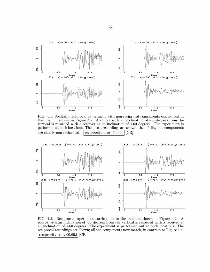
the components were oriented vertically and horizontally. Figure 4.3 shows complete seis-

mogram sections Xx,Xz, Zx and Zz recorded at the first location. The source extended

merely one grid point, thus the frequency content is quite high and resonance in the wave

field can be seen on all components. This pattern is mainly produced by the discretized

interface, which is represented in a stair-case manner. Each one of the stairs acts as a

scattering point for such high frequencies. At both locations I extracted single seismo-

grams. Figure 4.4 shows a plot of the four components of the received wave fields. Across

a row the receiver component is the same, while across a column the source component

is the same. In each quadrant two seismograms are overlaid, one at the left location (1),

the other at the right location (2). The diagonal plots show identical source and receiver

components, and the seismograms match perfectly. The off-diagonal plots clearly show

non-identical seismograms; the source component is different from the receiver component.

In this figure I extracted merely the traces at the reciprocal locations, but not the recip-

rocal components. On the off-diagonal plots one can see discrepancy in the traces starting

immediately at the first break; the mismatch extends until the end of the trace. One

can compare this result to Figure 4.5, where the off-diagonal components show a perfect

match. In contrast to Figure 4.4, reciprocal components are selected. All seismograms are

now reciprocal and match perfectly. In fact the two curves are indistinguishable. Thus,

the anisotropic elastic wave equation operator is symmetrically implemented using high-

order finite-differences on a staggered grid. Approximating the continuous wave equation

has not broken the original symmetry.

4.1.3 Spatially band-limited sources

The preceding example was generated with a spatially impulsive source that was activated

on the finite-difference grid. The spatial frequency content of the source thus generates

frequencies up to the spatial Nyquist frequency. Even for the highest frequencies, where the

finite-difference approximation becomes dispersive and inaccurate, numerical reciprocity

holds. However, dispersive artifacts caused by the numerical algorithm do not represent

wave propagation as it happens in nature. To remedy this problem one introduces sources

on a discrete grid not as a spatial impulses but rather in a band-limited manner. This

is aimed at reducing the spatial frequency content so that the difference operators can

approximate spatial derivatives accurately. If reciprocity has to be maintained, then a

-38-

FIG. 4.4. Spatially reciprocal experiment with non-reciprocal components carried out inthe medium shown in Figure 4.2. A source with an inclination of -60 degrees from thevertical is recorded with a receiver at an inclination of +60 degrees. The experiment isperformed at both locations. The direct recordings are shown; the off-diagonal components

are clearly non-reciprocal. reciprocity-drot.-60.60.i [CR]

FIG. 4.5. Reciprocal experiment carried out in the medium shown in Figure 4.2. Asource with an inclination of -60 degrees from the vertical is recorded with a receiver atan inclination of +60 degrees. The experiment is performed out at both locations. Thereciprocal recordings are shown; all the components now match, in contrast to Figure 4.4.

reciprocity-rrot.-60.60.i [CR]

-39-

spatially band-limited receiver must be used so that duality of the experiment is main-

tained.

To demonstrate, let P denote the staggered-grid finite-difference operator that propa-

gates the entire wave field; S, an operator that injects sources at certain locations in the

medium; R, a related operator that extracts the wave field at the receiver points. For

point sources and receivers, these two operators consist only of δ functions at the source

and receiver locations. For a source function f , the recorded data D are given by

D = R · P · S · f (4.14)

which in matrix form might appear schematically, like this:

D =

v1 v2 v3

v1 v2 v3. . .

. . .. . .

v1 v2 v3

. . . · · · .

.

.

.... . .

.

w1

w2 w1

w3 w2. . .

w3. . . w1. . . w2

w3

f.

(4.15)

Spatially band-limited receivers and sources can be implemented using appropriate weight

functions in the projection operators R and S. Multi-dimensional Gaussian weights are

commonly used. In equation (4.15), f denotes the vector of impulsive sources on the

gridded model, while P is the staggered-grid finite-difference modeling operator. Injection

and extraction operators S and R maintain reciprocity if they are transposes of each

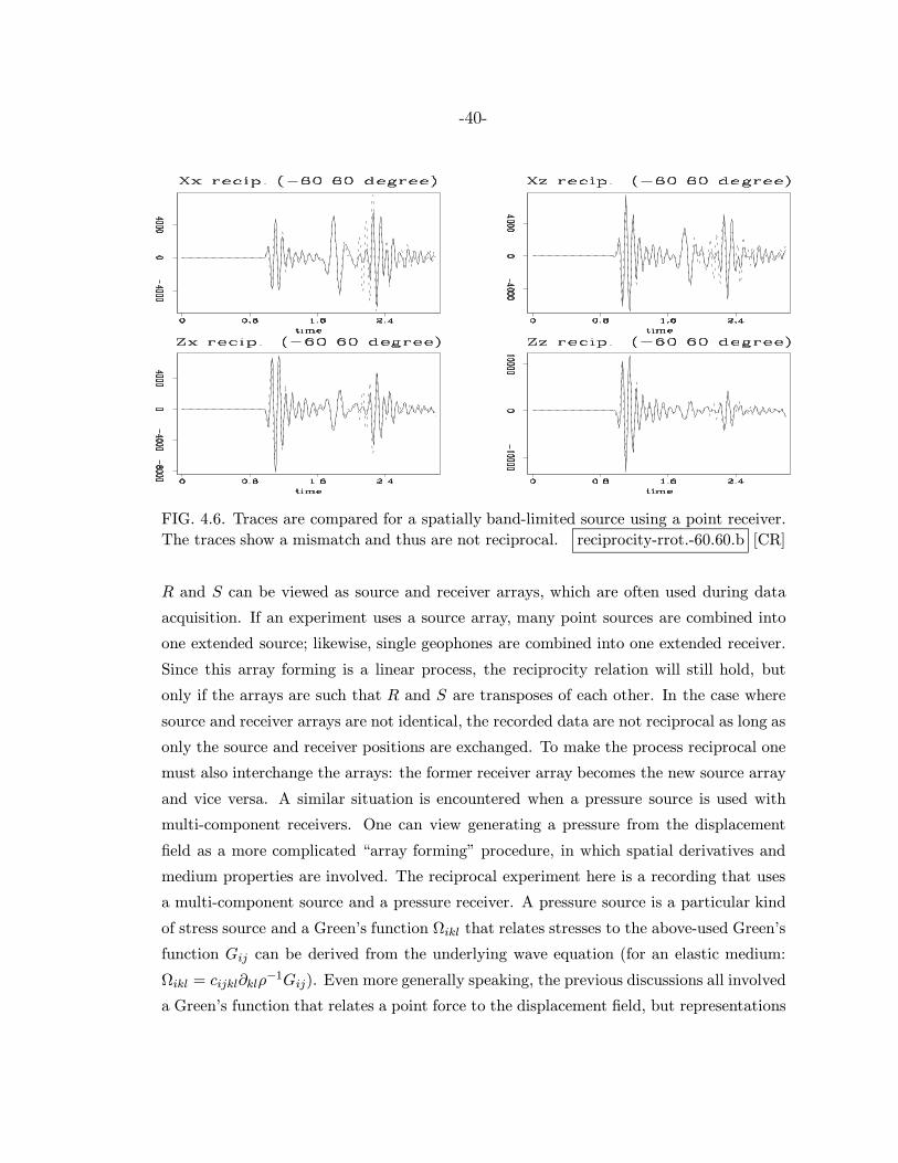
other, i.e., R = St. Figure 4.6 is an example of the use of a band-limited source, but

it uses point receivers and hence the result is not reciprocal. The Gaussian weight for

the source is of the form exp (−α[(x− x0)2 + (y − y0)2 + (z − z0)2]) and extends over a

four grid point half width. Mostly later arrivals are non-reciprocal on all components.

The application of the spatial source smoothing filter causes the entire finite-difference

propagation kernel to be unsymmetric. The frequency content is slightly lower since the

spatial filter couples with the time dimension through the wave equation and thus reduces

temporal frequency content as well. The data traces are matched remarkably well at

early times, more or less corresponding to the p-wave packet arrival, but deviations in

the waveform of the second wave packet, containing converted and diffracted energy, are

noticeable. If the receiver also is now spatially band-limited in the same way as the

source, reciprocity is again restored and the waveforms match exactly. The operators

-40-

FIG. 4.6. Traces are compared for a spatially band-limited source using a point receiver.

The traces show a mismatch and thus are not reciprocal. reciprocity-rrot.-60.60.b [CR]

R and S can be viewed as source and receiver arrays, which are often used during data

acquisition. If an experiment uses a source array, many point sources are combined into

one extended source; likewise, single geophones are combined into one extended receiver.

Since this array forming is a linear process, the reciprocity relation will still hold, but

only if the arrays are such that R and S are transposes of each other. In the case where

source and receiver arrays are not identical, the recorded data are not reciprocal as long as

only the source and receiver positions are exchanged. To make the process reciprocal one

must also interchange the arrays: the former receiver array becomes the new source array

and vice versa. A similar situation is encountered when a pressure source is used with

multi-component receivers. One can view generating a pressure from the displacement

field as a more complicated “array forming” procedure, in which spatial derivatives and

medium properties are involved. The reciprocal experiment here is a recording that uses

a multi-component source and a pressure receiver. A pressure source is a particular kind

of stress source and a Green’s function Ωikl that relates stresses to the above-used Green’s

function Gij can be derived from the underlying wave equation (for an elastic medium:

Ωikl = cijkl∂klρ−1Gij). Even more generally speaking, the previous discussions all involved

a Green’s function that relates a point force to the displacement field, but representations

-41-

can be found (Pao and Varatharajulu, 1976) that relate other quantities to the generated

displacement field. Those newly-created Green’s functions are all based on the same wave

equation and thus can be derived from each other.

In many cases of data processing, imaging, inversion, or optimization, reciprocity argu-

ments are invoked. If one follows such approaches, numerical implementations of operators

should be designed reciprocally. For example, the coarse-grid staggered finite-difference

wave equation operator in the preceding section is, when implemented conventionally, not

quite reciprocal. However, by symmetrizing the kernel, we can obtain complete reciprocity.

4.2 Consequences for seismic data

The recording of multicomponent seismic data is most often carried out over a limited

surface. The medium under investigation is parameterized by properties such as elastic

stiffnesses and density. Since we cannot know the medium completely, experiments are

designed to give us the best possible information. Realistically, seismic data are recorded

at sparse locations within the medium itself, never “at every point” in the medium. Thus

the complete Green’s tensor with total spatial coverage is impossible to obtain and will

always be band-limited.

For an elastic medium, such data will only approximate the Green’s tensor, even if they

are collected in a manner that spans the source and receiver component space. An ideal

experiment with multi-component sources and receivers should use at least three linearly

independent source directions and three linearly independent receiver directions. Then,

under ideal conditions, one records the full band-limited Green’s tensor, Gij i, j = 1, 2, 3,

for a given source-receiver pair.

Using fewer components may lead to ill-conditioned inversion and imaging results.

Types of such incomplete experiments can be a P-wave source recorded with three-

component receivers, which misses the other two wave types (SV and SH), or a vertical

source recorded into horizontal geophones, which misses the remaining components. One

is lucky if there are near-source wave-type conversions of such a nature that significant

amounts of the “originally missing” source-wave types are generated. However, in that

case, the experiment is not orthogonal, but rather a superposition of wave-type experi-

ments.

Knowing that reciprocity holds for arbitrary inhomogeneous, dispersive, and anisotropic

-42-

media, one can make use of the reciprocity relationship in various ways. The most com-

monly used practice is to reduce data acquisition by assuming ideal recording conditions.

Then only part of the data are collected and the rest are inferred by the invocation of

reciprocity relationships. Based on this assumption, one has only to collect GXy, GXz, and

GY z, in addition to GXx,GY y, and GZz, because by reciprocity GY x = GXy, GXz = GZx,

and GY z = GZy.

Another option is to claim that real world conditions are never ideal; then one would use

data redundancy to estimate other than material parameters, source or receiver variability,

or classification of noise sources. But in order to justify either approach, it is important

to determine the degree to which a real data set is “not reciprocal.” Thus, reciprocity

measurements give experimenters a much-needed sense of how accurate and reliable their

data are.

4.3 A real data example

The Pembrook data set has split-spread geometry and thus is ideal for comparing pairs

of (nearly) reciprocal traces. During the acquisition, no particular effort was made to

ensure that the employment of sources and geophones in the field was perfectly reciprocal.

In that respect, this data set represents a typical acquisition of multi-component data

in a production area. Surface-impact sources were used to acquire this data set. Such

sources are relatively weak compared to explosive sources. Consequently, each source was

activated not only once, but multiple times, and the resulting traces were stacked to create

the final field trace. Furthermore, each source was activated at an angle with respect to the

vertical, so that horizontal and vertical components were created by weighted subtraction

or addition.

Figures 4.7 – 4.10 show views of the prestack data set. Reciprocal behavior is more

easily detectable when one looks at prestack time slices than when one views the data in

other ways. Time slices are sensitive to small amplitude changes, and if data are normal-

moveout corrected, one can track a particular event within that time slice.

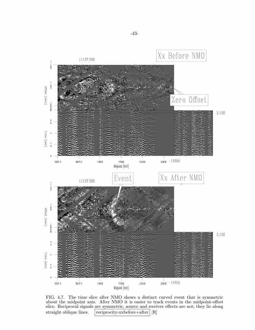
Figure 4.7 consists of two plots: the top plot shows the Xx component of the data,

while the lower plot shows the same data after normal moveout (NMO) correction. Both

plots use the same display style, which consists of three different panels. These panels

are three distinct faces in the prestack data cube, displayed in a flat manner. The cube

-43-

FIG. 4.7. The time slice after NMO shows a distinct curved event that is symmetricabout the midpoint axis. After NMO it is easier to track events in the midpoint-offsetslice. Reciprocal signals are symmetric, source and receiver effects are not; they lie along

straight oblique lines. reciprocity-xxbefore+after [R]

-44-

represents the whole data set spatially, but extends only 3-5 seconds in time. The faint

straight lines drawn on top of the panels indicate where in the cube the cut of the faces

was performed.

The top panel is a time slice at 3.12 seconds, where the midpoint axis is the horizontal

line in the middle of the slice. It is visible in the form of a few high amplitude traces

that traverse the entire slice horizontally. It also represents the dividing line between

negative and positive offsets, with the offset axis being exactly vertical. Negative offset

corresponds to the lower half of the slice; positive offset corresponds to the top half of the

slice. The panel below the time slice is a section of constant offset, since it is produced

by the cutting of the cube parallel to the midpoint axis. The farthest negative offset of

-11055 ft is shown. The panel to the right corresponds to a particular common midpoint

gather, where I cut the data cube at about a CMP location of 10500 ft.

For the lower plot, the location of displayed faces is identical to the top. In both plots,

before and after NMO, missing source and receiver positions are obvious. They manifest

themselves as dead traces in the constant offset section and CMP gather. In the time

slice these dead traces form patterns. Missing source and receiver locations are visible as

straight lines of zero amplitude at ±45 degree angles with respect to midpoint and offset

axis. Similarly, a few source and receiver consistent effects show up on parallel diagonal

lines.

Reciprocity should manifest itself in the prestack data cube by events that are sym-

metrical with respect to the midpoint axis. Before one applies NMO, this symmetry is

hardly observable, but after NMO, an event from a dipping reflector can be noticed be-

tween midpoint 14000 ft and 16000 ft. NMO approximately aligns the signal of this event

to show up in that time slice as a curved high amplitude event. The entire slice is clearly

not reciprocal, but some events in it show reciprocal behavior.

While Figure 4.7 displayed a prestack cube view of the entire data set for one single

(Xx) component, Figures 4.9 and 4.10 illustrate a particular time slice for all components

in the prestack data set. The time slice is cut at the identical time, where an event from

a dipping reflector is arriving. The 3 × 3 plots of reciprocal data are produced from the

original multi-component data cube given in the following manner:XxR XyR XzR

Y xR Y yR Y zR

ZxR ZyR ZzR

=

Xx Xy−|Y x+ Xz−|Zx+

Y x−|Xy+ Y y Y z−|Zy+

Zx−|Xz+ Zy−|Y z+ Zz

, (4.16)

-45-

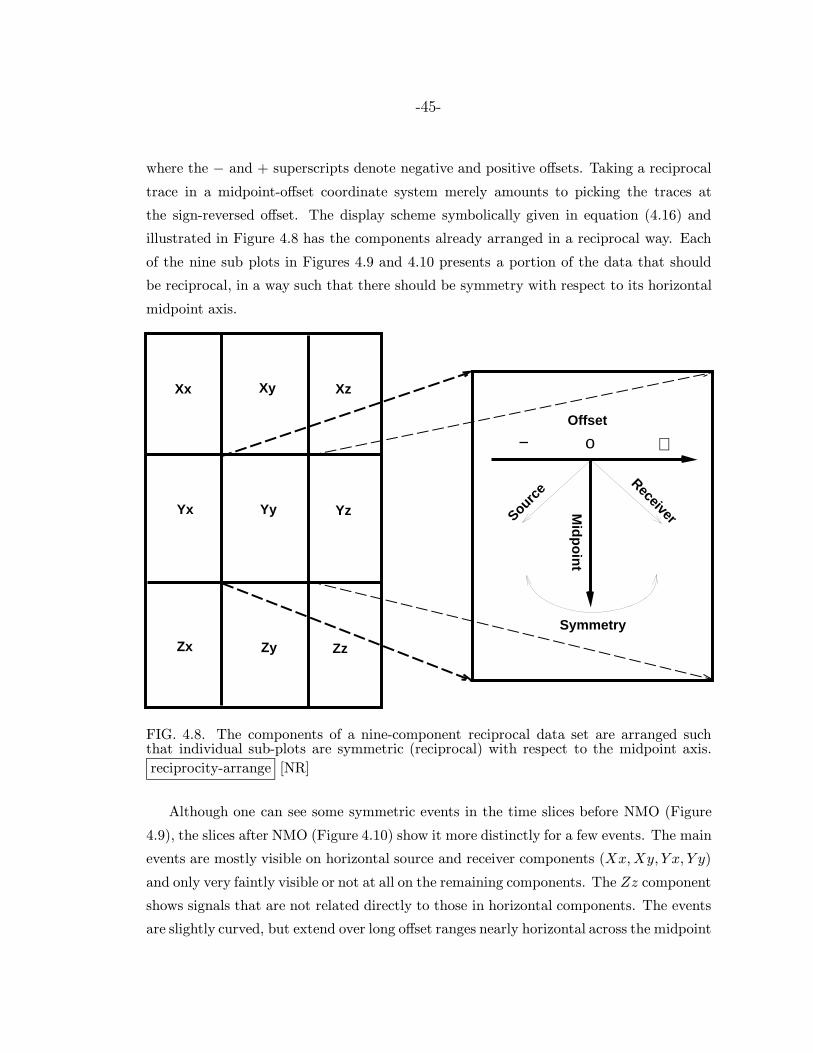
where the − and + superscripts denote negative and positive offsets. Taking a reciprocal

trace in a midpoint-offset coordinate system merely amounts to picking the traces at

the sign-reversed offset. The display scheme symbolically given in equation (4.16) and

illustrated in Figure 4.8 has the components already arranged in a reciprocal way. Each

of the nine sub plots in Figures 4.9 and 4.10 presents a portion of the data that should

be reciprocal, in a way such that there should be symmetry with respect to its horizontal

midpoint axis.

Xx Xy Xz

Yx Yy Yz

Zx Zy Zz

Offset

Midpoint

+− ο

Symmetry

ReceiverSource

FIG. 4.8. The components of a nine-component reciprocal data set are arranged suchthat individual sub-plots are symmetric (reciprocal) with respect to the midpoint axis.

reciprocity-arrange [NR]

Although one can see some symmetric events in the time slices before NMO (Figure

4.9), the slices after NMO (Figure 4.10) show it more distinctly for a few events. The main

events are mostly visible on horizontal source and receiver components (Xx,Xy, Y x, Y y)

and only very faintly visible or not at all on the remaining components. The Zz component

shows signals that are not related directly to those in horizontal components. The events

are slightly curved, but extend over long offset ranges nearly horizontal across the midpoint

-46-

axis; they are only a few midpoints wide and show some reciprocal behavior.

The remaining data are far from being reciprocal. Figure 4.11 shows zero-lag cross-

correlations of reciprocal trace pairs in the prestack data set. The correlations are com-

puted in a window from 3 to 4 seconds that contains the events shown in the previous

figures. The display of the sub-plots deviates from the general scheme, as given in Figure

4.8; that is only one half of the offset space is plotted, since those cross-correlations are

symmetric with respect to the midpoint axis. The correlations average events over a 1

second long window and thus give more robust indication of reciprocal signals. Those zero

lag correlations confirm the observations in the previous figures. Most reciprocal energy

is present at the spatial location of the main event in the time slice in Figure 4.10. Large

coherent zero-lag correlations are confined to the horizontal components and are dominant

on Xx and Y y. Horizontal and vertical cross-components hardly show any sign of spatially

coherent reciprocal signals. The Zz component shows large degrees of correlations which

are in agreement with the observation of thin curved events in Figure 4.9.

Although there are reciprocal events on some components in this prestack data volume,

the differences in reciprocal trace pairs are large. Such differences can have several causes:

for example, the uncertainty in source and receiver positioning, or the misalignment of

components. Another likely cause is that sources and receivers are not behaving identically

at each location. The multi-component source is activated regardless of the impedance of

the underlying ground, such that the level of energy transmitted into and extracted from

the ground is highly variable. Since source and receiver operate on the free surface, the

earth compliance can be highly directional and thus the energy transfer is not characterized

by a simple scalar quantity, but by an unknown time dependent and directional function.

4.4 Data processing and reciprocity

Some processing steps in seismic data analysis maintain reciprocity, while others may

result in data that are less reciprocal. All the processes applied in this thesis, e.g. muting

and t2 gain or normal moveout, maintain symmetry and thus reciprocity. Asymmetric

processing sequences can produce non-reciprocal data; on the other hand, however, the

resulting data might be more reciprocal after an asymmetric operation, if the process

manages to suppress non-reciprocal parts of the signal. Thus, if one is concerned about

-47-

FIG. 4.9. The time slice before NMO shows more events that are not symmetric withrespect to the midpoint axis. It is not easy to follow any one particular event in those

slices. reciprocity-beforereci [R]

-48-

FIG. 4.10. The time slice after NMO shows events that are symmetric with respect to themidpoint axis. It is easier to follow any one particular event after NMO in these slices.

reciprocity-afterreci [R]

-49-

FIG. 4.11. Reciprocal traces are correlated between 3 and 4 seconds traveltime for all ninecomponents. The midpoint axis is horizontal and the offset axis vertical. The highest cor-

relations coincide with the curved events in Figure 4.9 and 4.10. reciprocity-wnrecicorr

[R]

reciprocity or symmetry in seismic data, one ought to carefully consider the impact that

a data processing step might have on the symmetry of the seismic data.

4.5 Summary

Symmetrizing Green’s function kernels is important when using the elastic wave prop-

agation operators, as the above example of a non-reciprocal, but an accurate modeling

operator, shows. Numerical methods, properly developed, strictly obey the reciprocity

principle. In contrast to numerical simulations the real multi-component seismic data set

shows only a small degree of reciprocity for a few strong events, but exhibits otherwise

non-reciprocal behavior. Although all components are recorded in a nearly reciprocal ge-

ometry, the observed data are hardly reciprocal, which indicates a calibration problem

together with a large degree of near-source and near-receiver ground variability besides

the usual noise contamination in an active production area.