Temporal alignment and latent Gaussian processfactor inference in population spike trains

Lea Duncker & Maneesh SahaniGatsby Computational Neuroscience Unit

University College LondonLondon, W1T 4JG

{duncker,maneesh}@gatsby.ucl.ac.uk

Abstract

We introduce a novel scalable approach to identifying common latent structure inneural population spike-trains, which allows for variability both in the trajectoryand in the rate of progression of the underlying computation. Our approach isbased on shared latent Gaussian processes (GPs) which are combined linearly, asin the Gaussian Process Factor Analysis (GPFA) algorithm. We extend GPFA tohandle unbinned spike-train data by incorporating a continuous time point-processlikelihood model, achieving scalability with a sparse variational approximation.Shared variability is separated into terms that express condition dependence, aswell as trial-to-trial variation in trajectories. Finally, we introduce a nested GPformulation to capture variability in the rate of evolution along the trajectory. Weshow that the new method learns to recover latent trajectories in synthetic data, andcan accurately identify the trial-to-trial timing of movement-related parametersfrom motor cortical data without any supervision.

1 Introduction

Many computations in the brain are thought to be implemented by the dynamical evolution of activitydistributed across large neural populations. As simultaneous recordings of population activity havebecome more common, the need has grown for analytic methods that can identify these dynamicalcomputational variables from the data. Where the computation is tightly coupled to an externallymeasurable covariate — a stimulus or a movement, perhaps — such identification is a simple matterof exploiting linear or non-linear regression to describe a population encoding or decoding model.However, when aspects of the computation are likely to reflect internal mental states, which may varysubstantially even when external covariates remain constant, the relevant variables must be uncoveredfrom neural data alone, most typically using a latent variable model [1–6].

However, most such methods fail to account properly for at least one key form of dynamical variability— trial-to-trial differences in the timing of the computation. Such differences may be reflected inbehavioural variability, for instance in reaction times or movement durations [7], or in varyingrelationships between external events and neural firing, for instance in sensory onset latencies [8]. Insome cases manual alignment to salient external events or behavioural time-course may be used toreduce temporal misalignment [8, 9]. However, just as with variability in the trajectories themselves,temporal variations in purely internal states must ultimately be identified from neural data alone [10].

A particularly challenging problem is to build models that capture the variability both in the latenttrajectories underlying spiking population activity, and in the time-course with which such trajectoriesare followed. Temporal misalignment in trajectories might be confused for variability in the trajectoryitself; while genuine variability in that trajectory makes alignment more difficult. Indeed, previouswork has considered these problems separately. Algorithms like dynamic time warping (DTW) [11]

32nd Conference on Neural Information Processing Systems (NeurIPS 2018), Montréal, Canada.

treat the time-series as observed and try to estimate an optimal alignment of each series. DTW andrelated approaches may suffer in settings where observed data are noisy, though recent work hasbegun to explore more robust [12–15], or probabilistic alternatives for time-series alignment [16–18].Furthermore, these approaches generally assume a Gaussian noise model and often make assumptionsthat restrict applications to non-conjugate observation models. Only recently have studies consideredpairwise alignment of univariate [19–21], or multivariate point-processes [22]. Overall, simultaneousinference and temporal alignment of latent trajectories from multivariate point process observations –such as a set of spike-times of simultaneously recorded neurons – is a relatively unexplored area ofresearch.

In this work, we develop a novel method to jointly infer shared latent structure directly from thespiking activity of neural populations, allowing for (and identifying) trial-to-trial variations in thetiming of the latent processes. We make two main contributions.

First, we extend Gaussian Process Factor Analysis (GPFA) [2], an algorithm that has been successfullyapplied in the context of extracting time-varying low-dimensional latent structure from binned neuralpopulation activity on single trials, to directly model the point-process structure of spiking activity.We do so using a sparse variational approach, which both simplifies the adoption of a non-conjugatepoint-process likelihood, and significantly improves on the scalability of the GPFA algorithm.

Second, we combine the sparse variational GPFA model with a second Gaussian process in a nestedmodel architecture. We exploit shared latent structure across trials, or groups of trials, in order todisentangle variation in timing from variation in trajectories. This extension allows us to infer latenttime-warping functions that align trials in a purely unsupervised manner – that is, using populationspiking activity alone with no behavioural covariates. We apply our method to simulated data andshow that we can more accurately recover firing rate estimates than related methods. Using neural datafrom macaque monkeys performing a variable-delay centre-out reaching task, we demonstrate thatthe inferred alignment is behaviourally meaningful and predicts reaction times with high accuracy.

2 Gaussian Process Factor Analysis

Gaussian Process Factor Analysis (GPFA) is a method for inferring latent structure and single-trial trajectories in latent space that influence the firing of a population of neurons [2]. Temporalcorrelations in the high-dimensional neural population are modelled via a lower number of sharedlatent processes xk(·), k = 1, . . . ,K, which linearly relate to a high-dimensional signal hhh(·) ∈ RNin neural space. Thus, inter-trial variability in neural firing that is shared across the population ismodelled via the evolution of the latent processes on a given trial.

In the GPFA model, a Gaussian process (GP) prior is placed over each latent process xk(·), specifiedvia a mean function µk(·) and a covariance function, or kernel, κk(·, ·). The extent and nature of thetemporal correlations is specified by κk(·, ·) and governed via hyperparameters.

The classic GPFA model in [2] considers regularly sampled observations of hhh(t) that are corrupted byaxis-aligned Gaussian noise. Recent work has aimed to extend GPFA to a Poisson observation model[23]. Here, hhh(t) is related to a piecewise-constant firing rate of a Poisson process whose countingprocess is observed as spike-counts falling into time bins of a fixed width.

We can summarise the GPFA generative model for observations y(r)n (ti) of neuron n on trial r in a

general way by writing

x(r)k (·) ∼ GP(µk(·), κk(·, ·)) for k = 1, . . . ,K

h(r)n (·) =

K∑k=1

cn,kx(r)k (·) + dn for n = 1, . . . , N

y(r)n (ti) ∼ p(y(r)

n (ti)|h(r)n (ti)) for i = 1, . . . , T

(1)

The cn,k are weights for each latent and neuron that define a subspace mapping from low-dimensionallatent space to high-dimensional neural space and dn is a constant offset.

The widespread use of GPFA may be restricted by its poor scaling with time: Since time is evaluatedon an evenly spaced grid with T points, GPFA requires building and inverting a T × T covariancematrix, leading to O(T 3) complexity. The intractability of performing exact inference in GPFA

2

models with non-conjugate likelihood adds further complexity on top of this [23, 24]. In thenext section, we will outline how to improve the scalability of GPFA irrespective of the choice ofobservation model via the use of inducing points.

3 Sparse Variational Gaussian Process Factor Analysis (svGPFA)

The framework of sparse variational GP approximations [25] has helped to overcome difficultiesassociated with the scalability of GP methods to large sample sizes. It has since been applied todiverse problems in GP inference, contributing to improvements of the scalability of GP methods tolarge datasets and complex, potentially non-conjugate, applications [26–30].

A sparse variational extension of the GPFA model can be obtained by extending the work on additivesignal decomposition in [26]. The main idea is to augment the model in (1) by introducing inducingpointsuuuk for each latent process k = 1, . . . ,K. The inducing pointsuuuk represent function evaluationsof the kth latent GP at Mk input locations zzzk. A joint prior over the process xk(·) and its inducingpoints can hence be written as

p(uuuk|zzzk) = N(uuuk|000,K(k)

zz

)p(xk(·)|uuuk) = GP(µk(·), κk(·, ·))

(2)

where the GP prior over xk(·) is now conditioned on the inducing points with conditional mean andcovariance function

µk(t) = κκκk(t, zzz)K(k)zz

−1uuuk

κk(t, t′) = κk(t, t′)− κκκk(t, zzzk)K(k)zz

−1κκκk(zzzk, t

′)(3)

Here, κκκk(·, zzz) is a vector valued function taking a single input argument and consisting of evaluationsof the covariance function κk(·, ·) at the input and inducing point locations zzzk; K(k)

zz is the Grammatrix of κk(·, ·) evaluated at the inducing point locations.

We follow [26] in choosing a factorised variational approximation for posterior inference of theform q(uuu1:K , x1:K) =

∏Kk=1 p(xk|uuuk)q(uuuk), with Gaussian q(uuuk) = N (uuuk|mmmk, Sk). This choice

of posterior approximation makes it possible to derive a variational lower bound to the marginallog-likelihood over the observed data Y = {yyy(r)

1 , . . . , yyy(r)N }Rr=1 of the form

log p(Y) ≥R∑r=1

N∑n=1

Eq(h

(r)n )

[log p(yyy(r)

n |h(r)n )]−

R∑r=1

K∑k=1

KL[q(uuu

(r)k )‖p(uuu(r)

k )]def= F (4)

where q(h(r)n ) is the variational distribution over the affine transformation of the latents for the nth

neuron obtained from q(x) =∫p(x|uuu)q(uuu)duuu. q(h(r)

n ) is a GP with additive structure. Its meanfunction ν(r)

n (t) and covariance function σ(r)n (t, t′) are given by

ν(r)n (t) =

∑k

cn,k κκκk( t , zzzk) K(k)zz

−1mmm

(r)k + dn

σ(r)n (t, t′) =

∑k

c2n,k

(κk(t, t′) + κκκk(t, zzzk)

(K(k)zz

−1S

(r)k K(k)

zz

−1− K(k)

zz

−1)κκκk(zzzk, t

′)) (5)

The cost of evaluating this bound on the likelihood now scales linearly in the number of time pointsT , with cubic scaling only in the number of inducing points. Maximising the lower bound F in (4)allows for variational learning of the parameters in q(uuuk), the kernel hyperparmeters, the inducingpoint locations, and the model parameters describing the affine transformation from latents to hns.

3.1 A continuous-time point-process observation model

The form of the variational lower bound in (4) makes it clear that including different observationmodels only requires taking a Gaussian expectation of the respective log-likelihood. Importantly, theinference approach is essentially decoupled from the locations of the observed data. This crucial

3

consequence of the inducing point approach makes it possible to move away from gridded, binneddata and fully exploit the power of GPs in continuous-time.

Previous work has used sparse variational GP approximations to infer the intensity of a univariateGP modulated Poisson process [27]. Here, we extend this to the multivariate case by combiningthe svGPFA model with a point-process likelihood. To do this, we relate the affine transformationof the latent processes for the nth neuron, hn(·), to the non-negative intensity function of a point-process, λn(·), via a static non-linearity g : R→ R+. Thus, the spike times of neuron n on trial r,ttt(r)n = {t1, . . . tΦ(n,r)}, are modelled as

p(ttt(r)n |λ(r)n ) = exp

(−∫ Tr

0

dt λ(r)n (t)

)Φ(n,r)∏i=1

λ(r)n (ti) (6)

Where λn(t) = g(hn(t)), Tr is the duration of the rth trial, and Φ(n, r) is the total spike-count ofneuron n on trial r. The expected log-likelihood term in (4) can be evaluated as

Eq(h

(r)n )

[log p(ttt(r)n |h(r)

n )]

= −∫ Tr

0

Eq(h

(r)n )

[g(h(r)

n (t))]dt+

Φ(n,r)∑i=1

Eq(h

(r)n )

[log g(h(r)

n (ti))]

(7)

The resulting expected log-likelihood in (7) still contains an integral over the expected rate functionof the neuron, which cannot be computed analytically. However, the integral is one-dimensional andcan be computed numerically using efficient quadrature rules [31, 32].

The svGPFA model with point-process likelihood already fully addresses the two major limitations ofthe classic GPFA approach outlined in section 2: Firstly, it improves the scalability of the algorithmvia the use of inducing points, scaling cubically only in the number of inducing points per latentand linearly in the total number of spiking events. Secondly, our approach appropriately modelsneural spike trains as observations of a point-process. The model also provides the basis for furtherextensions addressing temporal alignment across trials, which will be the focus of the followingsection.

4 Temporal alignment and latent factor inference using Gaussian processes

The svGPFA model we have developed in section 3 aims to extract different latent trajectories on eachtrial. It does not explicitly model any structure that is shared across trials, and each trial’s variabletime-course is simply captured via inter-trial differences in latents. In this section, we will extendour basic svGPFA model in order to disentangle inter-trial variations in time-course from variationsin the latent trajectories themselves. To achieve this, we explicitly model latent structure that isshared across trials or subsets of trials, as well as structure that is specific to each trial, and makeuse of a nested GP architecture with time-warping functions. In this way, shared, neurally-definedlatent structure provides an anchor for the temporal alignment across trials. We extend the previousinducing point approach in order to arrive at a sparse variational inference algorithm in this setting.

4.1 A generative model for population spike times with grouped trial structure and variabletime courses

We introduce latent processes that are shared across all trials, across subsets of trials that share thesame experimental condition, or that are specific to each individual trial. We model each of these asdraws from a GP prior with K latent processes, L experimental conditions, and R trials:

shared: αk(·) ∼ GP(µαk (·), καk (·, ·)) for k = 1, . . . ,K

condition-specific: β(`)k (·) ∼ GP(µβk(·), κβk(·, ·)) for ` = 1, . . . , L

trial-specific: γ(r)k (·) ∼ GP(µγk(·), κγk(·, ·)) for r = 1, . . . , R

(8)

Allowing each of these latents to evolve in potentially separate subspaces, we define the linearmapping from low-dimensional latent, to high-dimensional neural space to be of the form

h(r)n (·) =

K∑k=1

(cαn,kαk(·) + cβn,kβ

`(r)k (·) + cγn,kγ

(r)k (·)

)+ dn (9)

4

(a)t

τ (r)

αk β(`)k γ

(r)k

λλλ(r)

hhh(r)

{ttt(r)n }Nn=1

Cα Cβ Cγ

g(·)

k = 1, . . . , K

r = 1, . . . , R

` = 1, . . . , L

(b) t

τ (r)

αk β(`)k γ

(r)k

λλλ(r)

{ttt(r)n }Nn=1

uuuτ,(r)

uuuαk uuuβ,(`)k uuu

γ,(r)k

hhh(r)

k = 1, . . . , K

r = 1, . . . , R

` = 1, . . . , L

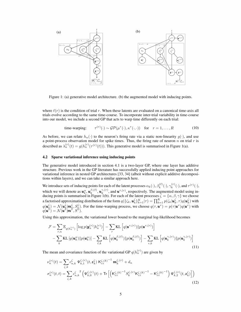
Figure 1: (a) generative model architecture. (b) the augmented model with inducing points.

where `(r) is the condition of trial r. When these latents are evaluated on a canonical time-axis alltrials evolve according to the same time-course. To incorporate inter-trial variability in time-courseinto our model, we include a second GP that acts to warp time differently on each trial:

time-warping: τ (r)(·) ∼ GP(µτ (·), κτ (·, ·)) for r = 1, . . . , R (10)

As before, we can relate hn(·) to the neuron’s firing rate via a static non-linearity g(·), and usea point-process observation model for spike times. Thus, the firing rate of neuron n on trial r isdescribed as λ(r)

n (t) = g(h(r)n (τ (r)(t))). This generative model is summarised in Figure 1(a).

4.2 Sparse variational inference using inducing points

The generative model introduced in section 4.1 is a two-layer GP, where one layer has additivestructure. Previous work in the GP literature has successfully applied inducing point approaches forvariational inference in nested GP architectures [33, 34] (albeit without explicit additive decomposi-tions within layers), and we can take a similar approach here.

We introduce sets of inducing points for each of the latent processes αk(·), β(`)k (·), γ(r)

k (·), and τ (r)(·),which we will denote as uuuαk , uuuβ,(`)k , uuuγ,(r)k , and uuuτ,(r), respectively. The augmented model using in-ducing points is summarised in Figure 1(b). For each of the latent processes ζ = {α, β, γ} we choosea factorised approximating distribution of the form q({ζk,uuuζk}Kk=1|τ) =

∏Kk=1 p(ζk|uuu

ζk, τ)q(uuuζk) with

q(uuuζk) = N (uuuζk|mmmζk, S

ζk). For the time-warping process, we choose q(τ,uuuτ ) = p(τ |uuuτ )q(uuuτ ) with

q(uuuτ ) = N (uuuτ |mmmτ , Sτ ).

Using this approximation, the variational lower bound to the marginal log-likelihood becomes

F =∑r,n

Eq(h

(r)n )

[log p(yyy(r)

n |h(r)n )]−∑r

KL[q(uuuτ,(r))‖p(uuuτ,(r))

]−∑k

KL [q(uuuαk )‖p(uuuαk )]−∑`,k

KL[q(uuu

β,(`)k )‖p(uuuβ,(`)k )

]−∑r,k

KL[q(uuu

γ,(r)k )‖p(uuuγ,(r)k )

](11)

The mean and covariance function of the variational GP q(h(r)n ) are given by

ν(r)n (t) =

∑ζ,k

cζn,k Ψζ,(r)k,1 (t, zzzζk) Kζ,(k)

zz

−1mmmζ,(r)k + dn

σ(r)n (t, t) =

∑ζ,k

cζn,k2(

Ψζ,(r)k,0 (t) + Tr

[(Kζ,(k)zz

−1Sζ,(r)k Kζ,(k)

zz

−1− Kζ,(k)

zz

−1)

Ψζ,(r)k,2 (t, zzzζk)

])(12)

5

The Ψζ,(r)k,i (t, zzzζk) are the Ψ-statistics [33, 35] of the kernel covariance functions

Ψζ,(r)k,0 (t) = Eq(τ(r))

[κκκζk( τ (r)(t) , τ (r)(t))

]Ψζ,(r)k,1 (t, zzzζk) = Eq(τ(r))

[κκκζk( τ (r)(t) , zzzζk)

]Ψζ,(r)k,2 (t, zzzζk) = Eq(τ(r))

[κκκζk(zzzζk, τ

(r)(t))κκκζk(τ (r)(t), zzzζk)] (13)

The Ψ-statistics can be evaluated analytically for common kernel choices such as the linear, ex-ponentiated quadratic, or cosine kernel. For other kernel choices they can be computed usinge.g. Gaussian quadrature. Finally, the variational distribution over the time-warping functionsq(τ (r)) =

∫p(τ (r)|uuuτ,(r))q(uuu(τ,(r))duuu(τ,(r) is also a GP with mean and covariance function

ντ,(r)(t) = κκκτ ( t , zzzτ ) Kτzz−1 mmmτ,(r)

στ,(r)(t, t′) = κτ (t, t′) + κκκτ (t, zzzτ )(Kτzz−1Sτ,(r)Kτzz

−1 − Kτzz−1)κκκτ (zzzτ , t′)

).

(14)

The variational lower bound in (11) can thus be evaluated tractably and optimised with respect to allparameters in the model. While the decomposition into shared, condition-specific and trial-specificlatents and the addition of the time-warping layer increases the total number of inducing points thatrequire optimisation, the impact on the time-complexity of the algorithm is minimal: it remains linearin the total number of spikes across trials and neurons, and only cubic in the number of inducingpoints per individual latent process.

5 Results

5.1 Synthetic data

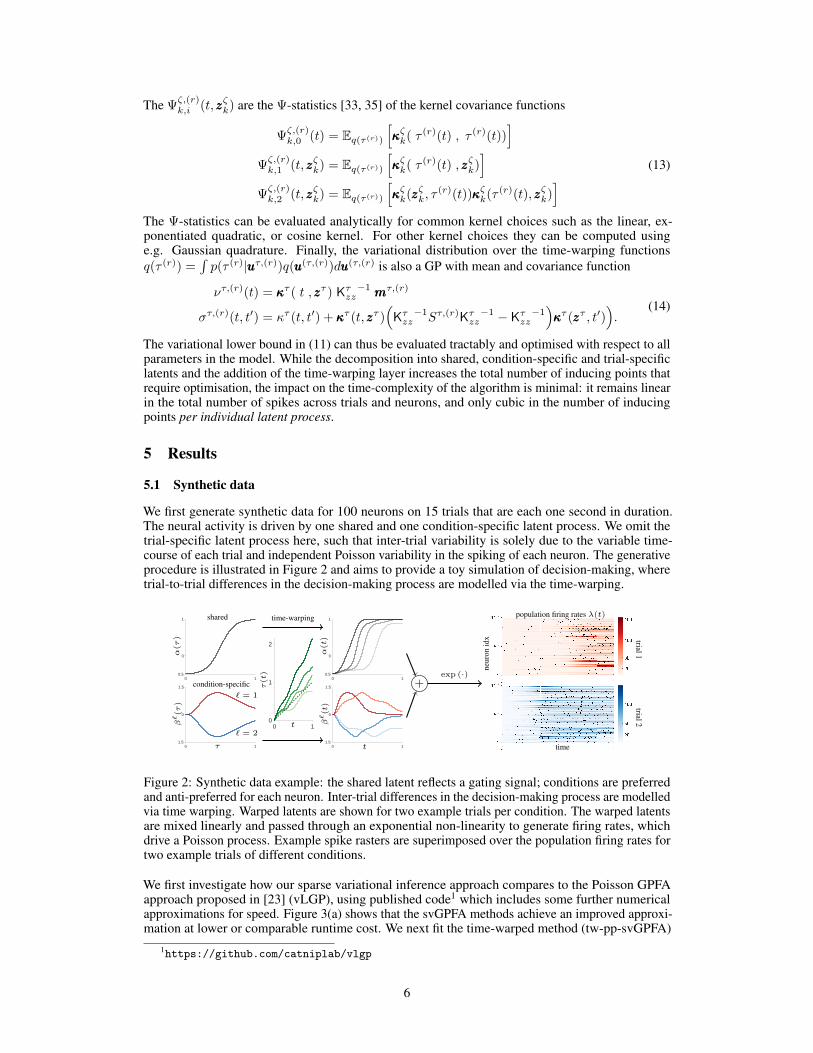
We first generate synthetic data for 100 neurons on 15 trials that are each one second in duration.The neural activity is driven by one shared and one condition-specific latent process. We omit thetrial-specific latent process here, such that inter-trial variability is solely due to the variable time-course of each trial and independent Poisson variability in the spiking of each neuron. The generativeprocedure is illustrated in Figure 2 and aims to provide a toy simulation of decision-making, wheretrial-to-trial differences in the decision-making process are modelled via the time-warping.

0 1-0.5

0

1

0 1-1.5

0

1.5

0 10

1

2

0 1-0.5

0

1

0 1-1.5

0

1.5 +

time-warping

exp (·)

τ t

β`(τ

)α(τ

)

β`(t)

α(t)

τ(t)

t

` = 1

` = 2

shared

condition-specific

time

neur

onid

x

population firing rates λ(t)

trial1trial2

Figure 2: Synthetic data example: the shared latent reflects a gating signal; conditions are preferredand anti-preferred for each neuron. Inter-trial differences in the decision-making process are modelledvia time warping. Warped latents are shown for two example trials per condition. The warped latentsare mixed linearly and passed through an exponential non-linearity to generate firing rates, whichdrive a Poisson process. Example spike rasters are superimposed over the population firing rates fortwo example trials of different conditions.

We first investigate how our sparse variational inference approach compares to the Poisson GPFAapproach proposed in [23] (vLGP), using published code1 which includes some further numericalapproximations for speed. Figure 3(a) shows that the svGPFA methods achieve an improved approxi-mation at lower or comparable runtime cost. We next fit the time-warped method (tw-pp-svGPFA)

1https://github.com/catniplab/vlgp

6

-2 0 2 4 6log(runtime)

2

6

10

nZ = 5nZ = 10nZ = 20nZ = 50nZ = 100vLGP

n.a. 1 5 10 20bin width in ms

2

5

20

25

RM

SE

P-svGPFApp-svGPFAtw-pp-svGPFAvLGPPLDStwPCA

n.a. 1 5 10 20bin width in ms

1

5

8

rela

tive

runt

ime

P-svGPFApp-svGPFAtw-pp-svGPFA

(a)

log

KL[q‖qfull]

(b) (c)

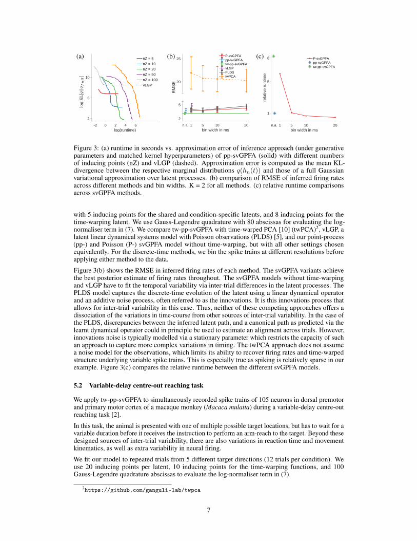
Figure 3: (a) runtime in seconds vs. approximation error of inference approach (under generativeparameters and matched kernel hyperparameters) of pp-svGPFA (solid) with different numbersof inducing points (nZ) and vLGP (dashed). Approximation error is computed as the mean KL-divergence between the respective marginal distributions q(hn(t)) and those of a full Gaussianvariational approximation over latent processes. (b) comparison of RMSE of inferred firing ratesacross different methods and bin widths. K = 2 for all methods. (c) relative runtime comparisonsacross svGPFA methods.

with 5 inducing points for the shared and condition-specific latents, and 8 inducing points for thetime-warping latent. We use Gauss-Legendre quadrature with 80 abscissas for evaluating the log-normaliser term in (7). We compare tw-pp-svGPFA with time-warped PCA [10] (twPCA)2, vLGP, alatent linear dynamical systems model with Poisson observations (PLDS) [5], and our point-process(pp-) and Poisson (P-) svGPFA model without time-warping, but with all other settings chosenequivalently. For the discrete-time methods, we bin the spike trains at different resolutions beforeapplying either method to the data.

Figure 3(b) shows the RMSE in inferred firing rates of each method. The svGPFA variants achievethe best posterior estimate of firing rates throughout. The svGPFA models without time-warpingand vLGP have to fit the temporal variability via inter-trial differences in the latent processes. ThePLDS model captures the discrete-time evolution of the latent using a linear dynamical operatorand an additive noise process, often referred to as the innovations. It is this innovations process thatallows for inter-trial variability in this case. Thus, neither of these competing approaches offers adissociation of the variations in time-course from other sources of inter-trial variability. In the case ofthe PLDS, discrepancies between the inferred latent path, and a canonical path as predicted via thelearnt dynamical operator could in principle be used to estimate an alignment across trials. However,innovations noise is typically modelled via a stationary parameter which restricts the capacity of suchan approach to capture more complex variations in timing. The twPCA approach does not assumea noise model for the observations, which limits its ability to recover firing rates and time-warpedstructure underlying variable spike trains. This is especially true as spiking is relatively sparse in ourexample. Figure 3(c) compares the relative runtime between the different svGPFA models.

5.2 Variable-delay centre-out reaching task

We apply tw-pp-svGPFA to simultaneously recorded spike trains of 105 neurons in dorsal premotorand primary motor cortex of a macaque monkey (Macaca mulatta) during a variable-delay centre-outreaching task [2].

In this task, the animal is presented with one of multiple possible target locations, but has to wait for avariable duration before it receives the instruction to perform an arm-reach to the target. Beyond thesedesigned sources of inter-trial variability, there are also variations in reaction time and movementkinematics, as well as extra variability in neural firing.

We fit our model to repeated trials from 5 different target directions (12 trials per condition). Weuse 20 inducing points per latent, 10 inducing points for the time-warping functions, and 100Gauss-Legendre quadrature abscissas to evaluate the log-normaliser term in (7).

2https://github.com/ganguli-lab/twpca

7

1 5 10

7

7.3

LON

O p

red-

logl

ik

104

warpednonwarped

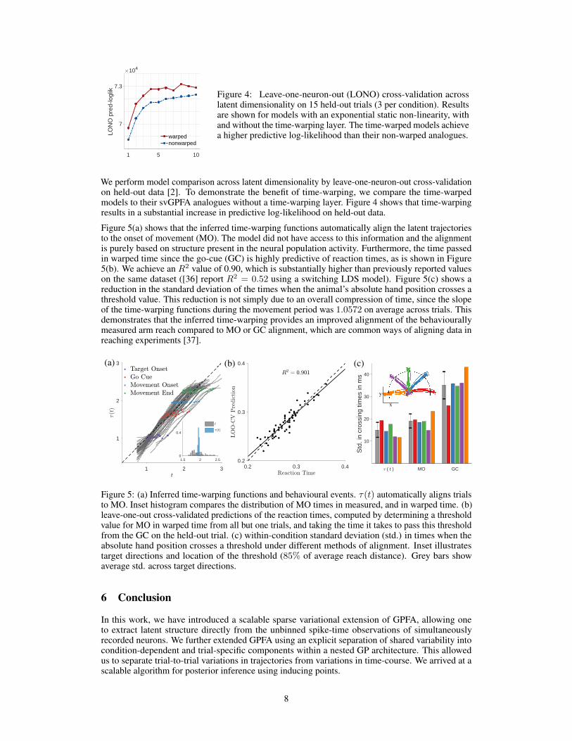
Figure 4: Leave-one-neuron-out (LONO) cross-validation acrosslatent dimensionality on 15 held-out trials (3 per condition). Resultsare shown for models with an exponential static non-linearity, withand without the time-warping layer. The time-warped models achievea higher predictive log-likelihood than their non-warped analogues.

We perform model comparison across latent dimensionality by leave-one-neuron-out cross-validationon held-out data [2]. To demonstrate the benefit of time-warping, we compare the time-warpedmodels to their svGPFA analogues without a time-warping layer. Figure 4 shows that time-warpingresults in a substantial increase in predictive log-likelihood on held-out data.

Figure 5(a) shows that the inferred time-warping functions automatically align the latent trajectoriesto the onset of movement (MO). The model did not have access to this information and the alignmentis purely based on structure present in the neural population activity. Furthermore, the time passedin warped time since the go-cue (GC) is highly predictive of reaction times, as is shown in Figure5(b). We achieve an R2 value of 0.90, which is substantially higher than previously reported valueson the same dataset ([36] report R2 = 0.52 using a switching LDS model). Figure 5(c) shows areduction in the standard deviation of the times when the animal’s absolute hand position crosses athreshold value. This reduction is not simply due to an overall compression of time, since the slopeof the time-warping functions during the movement period was 1.0572 on average across trials. Thisdemonstrates that the inferred time-warping provides an improved alignment of the behaviourallymeasured arm reach compared to MO or GC alignment, which are common ways of aligning data inreaching experiments [37].

1 2 3

1

2

3

1.5 2 2.50

0.4

0.2 0.3 0.40.2

0.3

0.4

( t ) MO GC

10

20

30

40

Std

. in

cros

sing

tim

es in

ms

(a) (b) (c)

y

x

Figure 5: (a) Inferred time-warping functions and behavioural events. τ(t) automatically aligns trialsto MO. Inset histogram compares the distribution of MO times in measured, and in warped time. (b)leave-one-out cross-validated predictions of the reaction times, computed by determining a thresholdvalue for MO in warped time from all but one trials, and taking the time it takes to pass this thresholdfrom the GC on the held-out trial. (c) within-condition standard deviation (std.) in times when theabsolute hand position crosses a threshold under different methods of alignment. Inset illustratestarget directions and location of the threshold (85% of average reach distance). Grey bars showaverage std. across target directions.

6 Conclusion

In this work, we have introduced a scalable sparse variational extension of GPFA, allowing oneto extract latent structure directly from the unbinned spike-time observations of simultaneouslyrecorded neurons. We further extended GPFA using an explicit separation of shared variability intocondition-dependent and trial-specific components within a nested GP architecture. This allowedus to separate trial-to-trial variations in trajectories from variations in time-course. We arrived at ascalable algorithm for posterior inference using inducing points.

8

Using synthetic data, we showed that our svGPFA methods can more accurately recover firingrate estimates than related methods. Using neural data, we demonstrated that our time-warpedmethod infers a behaviourally meaningful alignment in a completely unsupervised fashion using onlyinformation present in the neural population spike times. We showed that the inferred time-warpingis behaviourally meaningful, highly predictive of reaction times, and provides an improved temporalalignment compared to manually aligning to behaviourally defined time-points.

While we have focused on temporal variability in this work, we note that the inference scheme usinginducing points is more generally applicable for a variety of other nested GP models of interestin neuroscience, such as the GP-LVM [35, 38]. Similarly, further extensions of our model withtime-warping to deeper GP hierarchies – for instance using a non-linear mapping from latents toobservations as in the GP-LVM – can be incorporated straightforwardly.

The problem of latent input alignment in the context of the GP-LVM has also recently been consideredin [39], where maximum a posteriori inference in a Gaussian model is used to recover a single trueunderlying input sequence from multiple observations that are generated from different time-warpingfunctions. The sparse-variational approach we have presented here could hence be used to generalisethis approach to account for further differences across sequences, and extend it to non-Gaussiansettings.

Furthermore, our approach can also be applied to multiple sets of observed data with potentiallydifferent likelihoods in a canonical correlations analysis extension of GPFA. This could be usefulfor inferring latent structure from multiple recorded signals. For instance, one could combine theanalysis of LFP or calcium imaging data with that of spike trains. Thus, with slight modifications tothe model architecture, an analogous inference approach to the one presented here is applicable in avariety of contexts, including manifold learning, combinations of modalities, and beyond.

Acknowledgements

We would like to thank Vincent Adam for early contributions to this project, Gergö Bohner for helpfuldiscussions, and the Shenoy laboratory at Stanford University for sharing the centre-out reachingdataset. This work was funded by the Simons Foundation (SCGB 323228, 543039; MS) and theGatsby Charitable Foundation.

References[1] MM Churchland, BM Yu, M Sahani, and KV Shenoy. Techniques for extracting single-trial activity

patterns from large-scale neural recordings. Current Opinion in Neurobiology, 17(5):609–618, 2007.

[2] BM Yu, JP Cunningham, G Santhanam, SI Ryu, KV Shenoy, and M Sahani. Gaussian-process factoranalysis for low-dimensional single-trial analysis of neural population activity. Journal of Neurophysiology,102(1):614–635, 2009.

[3] Y Gao, EW Archer, L Paninski, and JP Cunningham. Linear dynamical neural population models throughnonlinear embeddings. In Advances in Neural Information Processing Systems, pp. 163–171, 2016.

[4] C Pandarinath, DJ O’Shea, J Collins, R Jozefowicz, SD Stavisky, JC Kao, EM Trautmann, MT Kaufman,SI Ryu, LR Hochberg, JM Henderson, KV Shenoy, LF Abbott, and D Sussillo. Inferring single-trial neuralpopulation dynamics using sequential auto-encoders. Nature Methods, 15(10):805–815, 2018.

[5] JH Macke, L Buesing, and M Sahani. Estimating state and parameters in state space models of spike trains.Advanced State Space Methods for Neural and Clinical Data, p. 137, 2015.

[6] JP Cunningham and BM Yu. Dimensionality reduction for large-scale neural recordings. Nature Neuro-science, 17(11):1500–1509, 2014.

[7] A Afshar, G Santhanam, BM Yu, SI Ryu, M Sahani, and KV Shenoy. Single-trial neural correlates of armmovement preparation. Neuron, 71(3):555–564, 2011.

[8] S Kollmorgen and RH Hahnloser. Dynamic alignment models for neural coding. PLoS computationalbiology, 10(3):e1003508, 2014.

[9] PN Lawlor, MG Perich, LE Miller, and KP Kording. Linear-nonlinear-time-warp-poisson models of neuralactivity. Journal of Computational Neuroscience, 2018.

[10] B Poole, A Williams, N Maheswaranathan, BM Yu, G Santhanam, S Ryu, SA Baccus, K Shenoy, andS Ganguli. Time-warped PCA: simultaneous alignment and dimensionality reduction of neural data. InFrontiers in Neuroscience. Computational and Systems Neuroscience (COSYNE), Salt Lake City, UT, 2017.

9

[11] H Sakoe and S Chiba. Dynamic programming algorithm optimization for spoken word recognition. IEEETransactions on Acoustics, Speech, and Signal Processing, 26(1):43–49, 1978.

[12] EJ Keogh and MJ Pazzani. Derivative dynamic time warping. In Proceedings of the 2001 SIAM Interna-tional Conference on Data Mining, pp. 1–11. SIAM, 2001.

[13] E Hsu, K Pulli, and J Popovic. Style translation for human motion. In ACM Transactions on Graphics(TOG), vol. 24, pp. 1082–1089. ACM, 2005.

[14] M Cuturi and M Blondel. Soft-DTW: a differentiable loss function for time-series. In Proceedings of the34th International Conference on Machine Learning, pp. 894–903, 2017.

[15] F Zhou and F De la Torre. Generalized canonical time warping. IEEE Transactions on Pattern Analysisand Machine Intelligence, 38(2):279–294, 2016.

[16] M Lázaro-Gredilla. Bayesian warped Gaussian processes. In F Pereira, CJC Burges, L Bottou, andKQ Weinberger, eds., Advances in Neural Information Processing Systems 25, pp. 1619–1627. CurranAssociates, Inc., 2012.

[17] J Snoek, K Swersky, R Zemel, and R Adams. Input warping for Bayesian optimization of non-stationaryfunctions. In Proceedings of the 31st International Conference on Machine Learning, pp. 1674–1682,2014.

[18] M Kaiser, C Otte, T Runkler, and CH Ek. Bayesian alignments of warped multi-output Gaussian processes.arXiv preprint arXiv:1710.02766, 2017.

[19] A Arribas-Gil and HG Müller. Pairwise dynamic time warping for event data. Computational Statistics &Data Analysis, 69:255–268, 2014.

[20] VM Panaretos, Y Zemel, et al. Amplitude and phase variation of point processes. The Annals of Statistics,44(2):771–812, 2016.

[21] W Wu and A Srivastava. Estimating summary statistics in the spike-train space. Journal of ComputationalNeuroscience, 34(3):391–410, 2013.

[22] Y Zemel and VM Panaretos. Fréchet means and procrustes analysis in wasserstein space. arXiv preprintarXiv:1701.06876, 2017.

[23] Y Zhao and IM Park. Variational latent Gaussian process for recovering single-trial dynamics frompopulation spike trains. Neural Computation, 29(5):1293–1316, 2017.

[24] M Opper and C Archambeau. The variational Gaussian approximation revisited. Neural Computation,21(3):786–792, 2009.

[25] MK Titsias. Variational learning of inducing variables in sparse Gaussian processes. In Proceedings of the12th International Conference on Artificial Intelligence and Statistics, pp. 567–574, 2009.

[26] V Adam, J Hensman, and M Sahani. Scalable transformed additive signal decomposition by non-conjugateGaussian process inference. In Proceedings of the 26th International Workshop on Machine Learning forSignal Processing (MLSP), 2016.

[27] C Lloyd, T Gunter, MA Osborne, and SJ Roberts. Variational inference for Gaussian process modulatedPoisson processes. In Proceedings of the 32nd International Conference on Machine Learning, 2015.

[28] J Hensman, N Fusi, and ND Lawrence. Gaussian processes for big data. In Conference on Uncertainty inArtificial Intellegence, pp. 282–290. auai.org, 2013.

[29] J Hensman, AGdG Matthews, and Z Ghahramani. Scalable variational Gaussian process classification. InProceedings of the 18th International Conference on Artificial Intelligence and Statistics, 2015.

[30] AD Saul, J Hensman, A Vehtari, and ND Lawrence. Chained Gaussian processes. In Proceedings of the19th International Conference on Artificial Intelligence and Statistics, pp. 1431–1440, 2016.

[31] G Mena and L Paninski. On quadrature methods for refractory point process likelihoods. NeuralComputation, 26(12):2790–2797, 2014.

[32] P Abbott. Tricks of the trade: Legendre-gauss quadrature. Mathematica Journal, 9(4):689–691, 2005.

[33] A Damianou and N Lawrence. Deep Gaussian processes. In Proceedings of the 16th InternationalConference on Artificial Intelligence and Statistics, pp. 207–215, 2013.

[34] H Salimbeni and M Deisenroth. Doubly stochastic variational inference for deep Gaussian processes. InAdvances in Neural Information Processing Systems, pp. 4591–4602, 2017.

[35] MK Titsias and ND Lawrence. Bayesian Gaussian process latent variable model. In Proceedings of the13th International Conference on Artificial Intelligence and Statistics, pp. 844–851, 2010.

[36] B Petreska, BM Yu, JP Cunningham, G Santhanam, SI Ryu, KV Shenoy, and M Sahani. Dynamicalsegmentation of single trials from population neural data. In Advances in Neural Information ProcessingSystems, pp. 756–764, 2011.

10

[37] MM Churchland, JP Cunningham, MT Kaufman, JD Foster, P Nuyujukian, SI Ryu, and KV Shenoy.Neural population dynamics during reaching. Nature, 487(7405):51, 2012.

[38] A Wu, NG Roy, S Keeley, and JW Pillow. Gaussian process based nonlinear latent structure discoveryin multivariate spike train data. In Advances in Neural Information Processing Systems, pp. 3499–3508,2017.

[39] I Kazlauskaite, CH Ek, and ND Campbell. Gaussian process latent variable alignment learning. arXivpreprint arXiv:1803.02603, 2018.

11